to the critically acclaimed assassin’s creed game · assassin’s creed 4 is a historical...
TRANSCRIPT
1

Assassin’s Creed 4 is a historical action-adventure video game set in seventeenth century, golden age of piracy and placed in vast open world of Caribbean Sea area.
It is in fact the sixth installment to the critically acclaimed Assassin’s Creed game franchise, but the new setting and historic period presented several new challenges:
• Multiple environment types
• Small islands and non-habited beaches
• Densely populated cities
• Deep jungles
• Open world of Caribbean Sea
• Dynamically changing and unpredictable tropical weather and various atmospheric phenomena – rain storms, mist, fog, god rays
• Very small number of artificial light sources and need to achieve interesting and complex lighting using only natural light
Our game targeted six different hardware platforms, including the next-generation consoles - Microsoft Xbox One and Sony PlayStation 4.
I’m going to cover what we achieved using new capabilities and available power of this hardware, while still maintaining consistent art direction between all the target platforms.
2
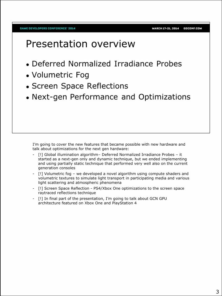
I’m going to cover the new features that became possible with new hardware and talk about optimizations for the next gen hardware:
- [!] Global illumination algorithm– Deferred Normalized Irradiance Probes – it started as a next-gen only and dynamic technique, but we ended implementing and using partially static technique that performed very well also on the current generation consoles
- [!] Volumetric fog – we developed a novel algorithm using compute shaders and volumetric textures to simulate light transport in participating media and various light scattering and atmospheric phenomena
- [!] Screen Space Reflection - PS4/Xbox One optimizations to the screen space raytraced reflections technique
- [!] In final part of the presentation, I’m going to talk about GCN GPU architecture featured on Xbox One and PlayStation 4
3
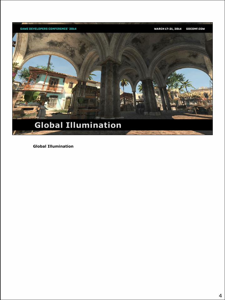
Global Illumination
4
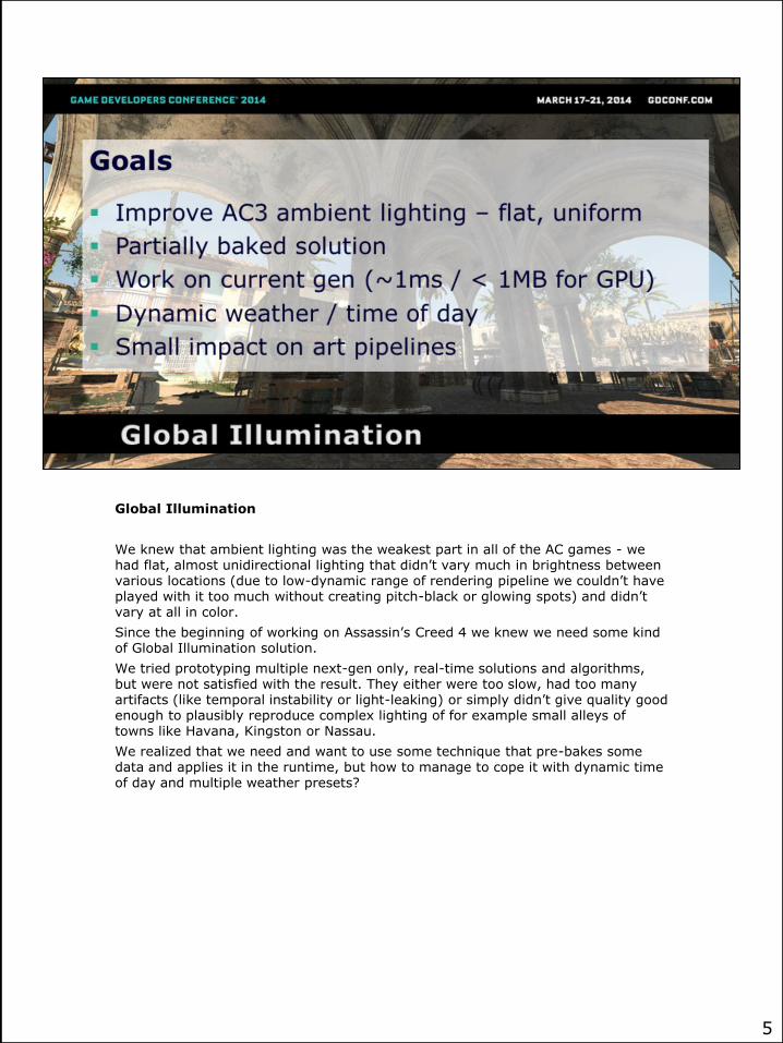
Global Illumination
We knew that ambient lighting was the weakest part in all of the AC games - we had flat, almost unidirectional lighting that didn’t vary much in brightness between various locations (due to low-dynamic range of rendering pipeline we couldn’t have played with it too much without creating pitch-black or glowing spots) and didn’t vary at all in color.
Since the beginning of working on Assassin’s Creed 4 we knew we need some kind of Global Illumination solution.
We tried prototyping multiple next-gen only, real-time solutions and algorithms, but were not satisfied with the result. They either were too slow, had too many artifacts (like temporal instability or light-leaking) or simply didn’t give quality good enough to plausibly reproduce complex lighting of for example small alleys of towns like Havana, Kingston or Nassau.
We realized that we need and want to use some technique that pre-bakes some data and applies it in the runtime, but how to manage to cope it with dynamic time of day and multiple weather presets?
5

Deferred Normalized Irradiance Probes
Key observations:
- Under sunny weather usually most perceived indirect lighting comes from main light source
- We can easily split indirect lighting from sky and it’s bounces from main light component – techniques existing in our engine (like World Ambient Occlusion and SSAO) are enough to provide shadowing information
- Main light trajectory not dependent on weather preset – only light color and strength depends on it
- We can factor out light color and intensity from light transfer functions
- For a single GI diffuse-only bounce we can precompute and store “some” information based only on:
- Albedo
- Normals
- Shadowing information
6
7

8
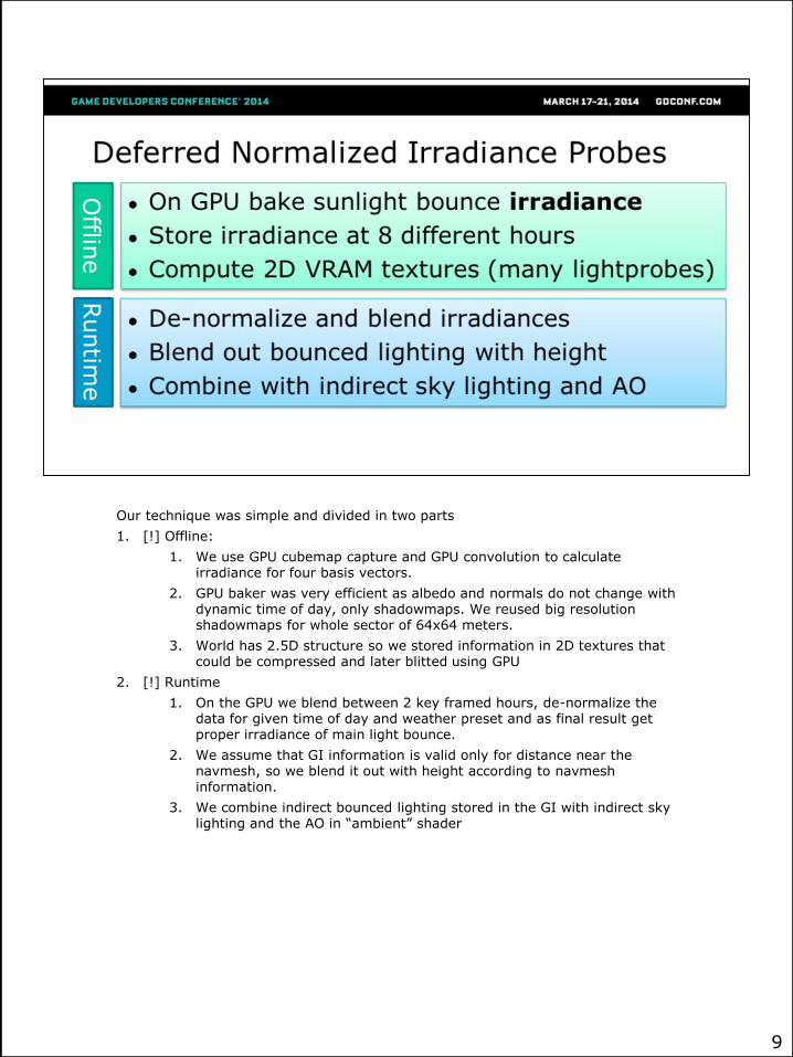
Our technique was simple and divided in two parts
1. [!] Offline:
1. We use GPU cubemap capture and GPU convolution to calculate irradiance for four basis vectors.
2. GPU baker was very efficient as albedo and normals do not change with dynamic time of day, only shadowmaps. We reused big resolution shadowmaps for whole sector of 64x64 meters.
3. World has 2.5D structure so we stored information in 2D textures that could be compressed and later blitted using GPU
2. [!] Runtime
1. On the GPU we blend between 2 key framed hours, de-normalize the data for given time of day and weather preset and as final result get proper irradiance of main light bounce.
2. We assume that GI information is valid only for distance near the navmesh, so we blend it out with height according to navmeshinformation.
3. We combine indirect bounced lighting stored in the GI with indirect sky lighting and the AO in “ambient” shader
9

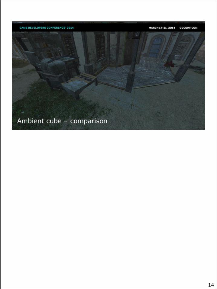
Old AC3 technique – just the ambient cube. (screenshot doesn’t have the AO part, just pure ambient lighting)
Screenshot from around 7-8PM, because of very low sun elevation this part of town is completely in shadow.
Effect – uninteresting, artificial look. Loss of almost all normal mapping and lighting variety.
It is also too dark, but brighter values would result in even flatter look.
10
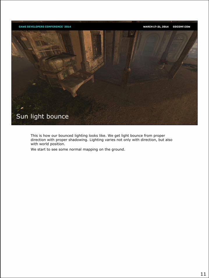
This is how our bounced lighting looks like. We get light bounce from proper direction with proper shadowing. Lighting varies not only with direction, but also with world position.
We start to see some normal mapping on the ground.
11
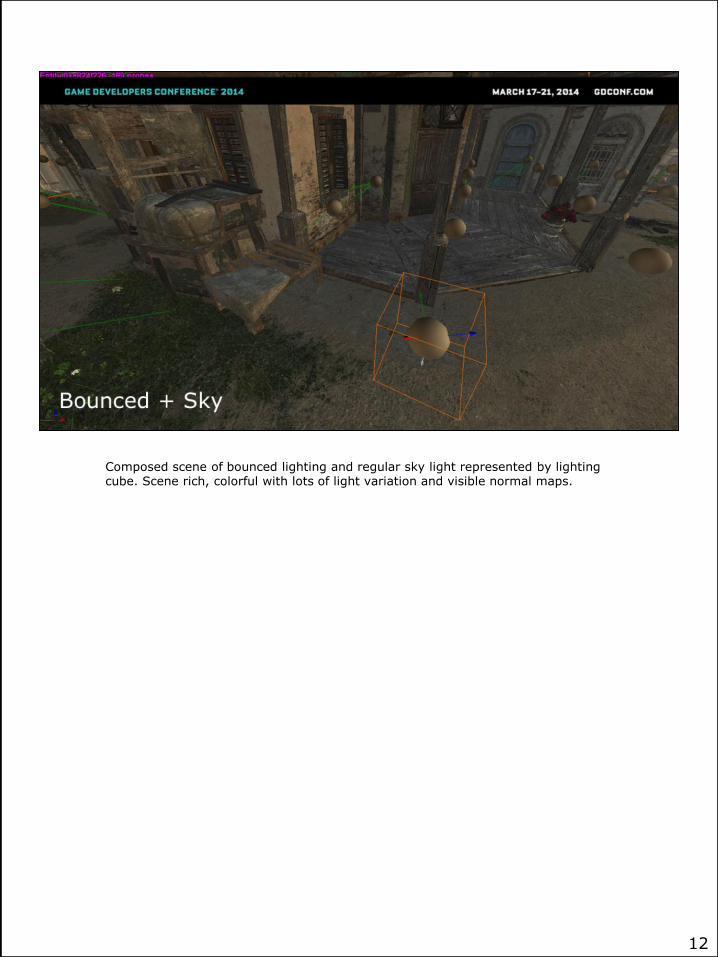
Composed scene of bounced lighting and regular sky light represented by lighting cube. Scene rich, colorful with lots of light variation and visible normal maps.
12
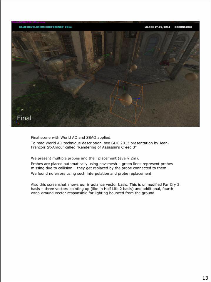
Final scene with World AO and SSAO applied.
To read World AO technique description, see GDC 2013 presentation by Jean-Francois St-Amour called “Rendering of Assassin’s Creed 3”
We present multiple probes and their placement (every 2m).
Probes are placed automatically using nav-mesh – green lines represent probes missing due to collision – they get replaced by the probe connected to them.
We found no errors using such interpolation and probe replacement.
Also this screenshot shows our irradiance vector basis. This is unmodified Far Cry 3 basis – three vectors pointing up (like in Half Life 2 basis) and additional, fourth wrap-around vector responsible for lighting bounced from the ground.
13
14
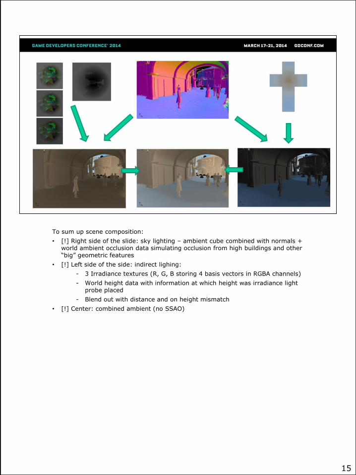
To sum up scene composition:
• [!] Right side of the slide: sky lighting – ambient cube combined with normals + world ambient occlusion data simulating occlusion from high buildings and other “big” geometric features
• [!] Left side of the side: indirect lighing:
- 3 Irradiance textures (R, G, B storing 4 basis vectors in RGBA channels)
- World height data with information at which height was irradiance light probe placed
- Blend out with distance and on height mismatch
• [!] Center: combined ambient (no SSAO)
15
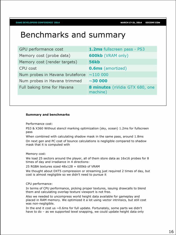
Summary and benchmarks
Performance cost:
PS3 & X360 Without stencil marking optimization (sky, ocean) 1.2ms for fullscreenpass
When combined with calculating shadow mask in the same pass, around 1.8ms
On next gen and PC cost of bounce calculations is negligible compared to shadow mask that it is computed with
Memory cost:
We load 25 sectors around the player, all of them store data as 16x16 probes for 8 times of day and irradiance in 4 directions:
25 RGBA textures sized 48x128 = 600kb of VRAM
We thought about DXT5 compression or streaming just required 2 times of day, but cost is almost negligible so we didn’t need to pursue it
CPU performance:
In terms of CPU performance, picking proper textures, issuing drawcalls to blend them and calculating overlap texture viewport is not free.
Also we needed to uncompress world height data available for gameplay and placed in RAM memory. We optimized it a lot using vector intrinsics, but still cost was non-negligible.
In the end it cost us ~0.6ms for full update. Fortunately, some parts we didn’t have to do – as we supported texel snapping, we could update height data only
16

when it was needed.
Number of probes:
When using bruteforce placement on lowest available spot in the world aligned to grid, we had around 110 000 probes per typical game world.
When we used navigation mesh to place probes only on areas accessible to the player, it got down to 30 000.
Full baking time:
On single machine equipped with nVidia GTX 680, full baking time for whole world and all 8 times of day was around 8 minutes. Therefore it didn’t require any distribution over whole world, technical art directors and lighting artists were able to trigger it on demand.
We also added option to re-bake some probes or have continuous baking in background in editor (probes visible in the viewport were constantly rebaked in the background – almost no performance impact)
16
Volumetric Fog
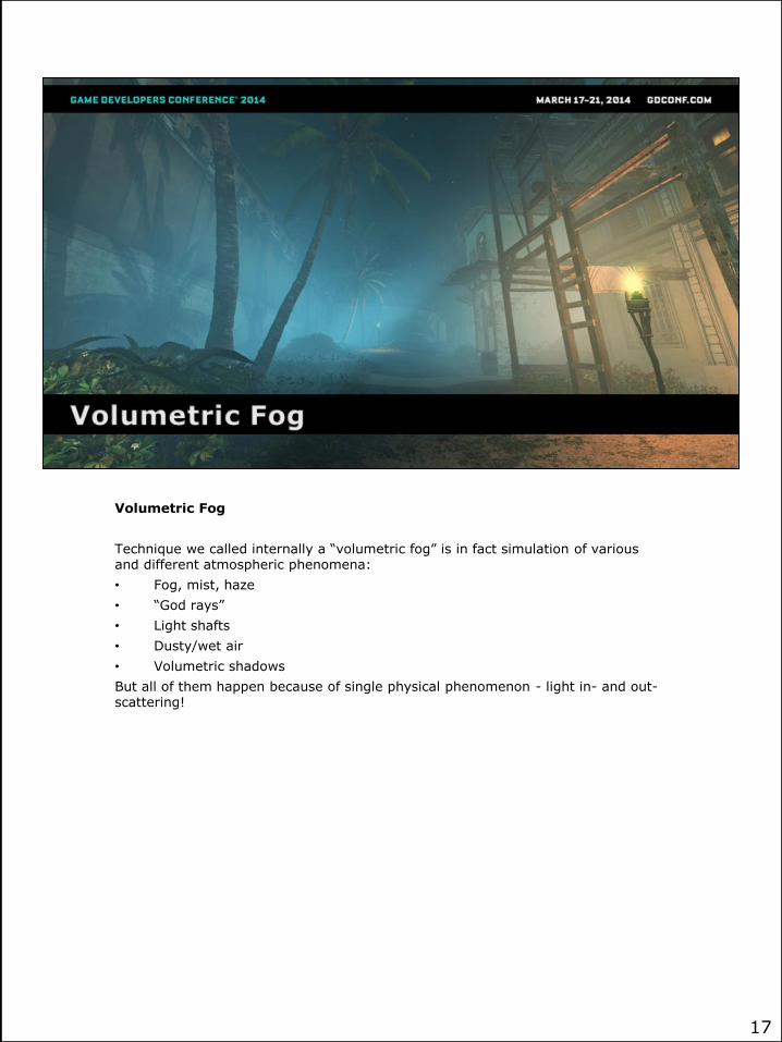
Technique we called internally a “volumetric fog” is in fact simulation of various and different atmospheric phenomena:
• Fog, mist, haze
• “God rays”
• Light shafts
• Dusty/wet air
• Volumetric shadows
But all of them happen because of single physical phenomenon - light in- and out-scattering!
17
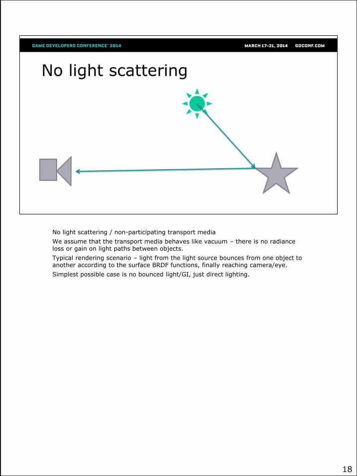
No light scattering / non-participating transport media
We assume that the transport media behaves like vacuum – there is no radiance loss or gain on light paths between objects.
Typical rendering scenario – light from the light source bounces from one object to another according to the surface BRDF functions, finally reaching camera/eye.
Simplest possible case is no bounced light/GI, just direct lighting.
18
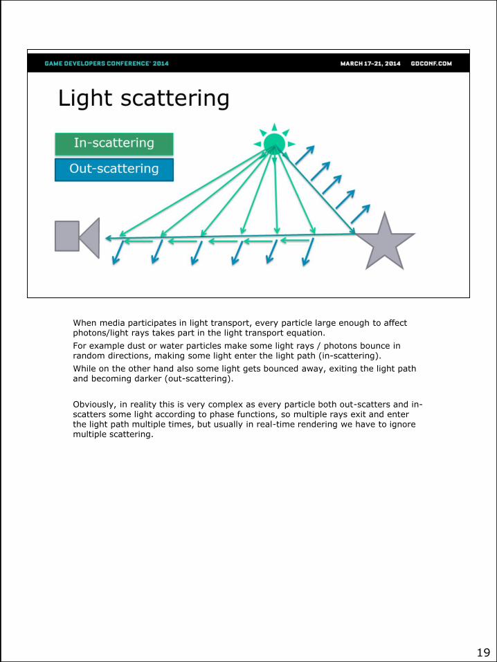
When media participates in light transport, every particle large enough to affect photons/light rays takes part in the light transport equation.
For example dust or water particles make some light rays / photons bounce in random directions, making some light enter the light path (in-scattering).
While on the other hand also some light gets bounced away, exiting the light path and becoming darker (out-scattering).
Obviously, in reality this is very complex as every particle both out-scatters and in-scatters some light according to phase functions, so multiple rays exit and enter the light path multiple times, but usually in real-time rendering we have to ignore multiple scattering.
19
[!] Light scattering effect is not always clearly visible and in many cases it can be ignored. Its visibility depends on:
- Media – for example air/water/steam/milk have different media particle sizes.
- Distance – it is easy to see light scattering on distant mountains, it’s difficult to notice any effect in clean air in couple meters range.
- Light angle – scattering phase functions cause sky look blue at noon and orange/pink at dusk/dawn.
- Weather conditions – in fact different weather means different sized particles in the air – for example more dust or steam/water.
- Light occlusion – if light is shadowed, it cannot contribute to light in-scattering –this is what creates interesting light-shaft effect.
[!] Problem is very difficult to solve, as scattering equation is a differential equation and it’s solution is a calculus that cannot be solved analytically for “any” scattering media, shadowing and conditions.
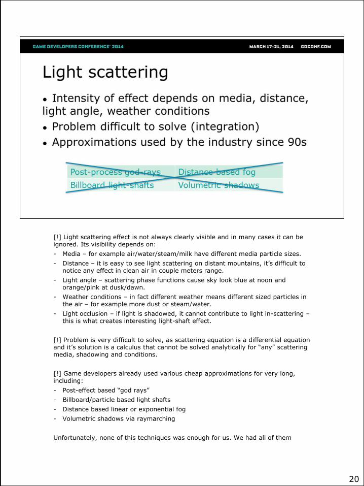
[!] Game developers already used various cheap approximations for very long, including:
- Post-effect based “god rays”
- Billboard/particle based light shafts
- Distance based linear or exponential fog
- Volumetric shadows via raymarching
Unfortunately, none of this techniques was enough for us. We had all of them
20

working, but the problem was that all of them were separate techniques. We wanted to have an unified, physically based solution that would combine all of them, allow us to achieve visual consistency, and would mean no tedious work and set-up for artists.
20

After prototyping numerous “classic” techniques, our biggest inspiration came from “Light Propagation Volumes” GI technique by Anton Kaplanyan presented at Siggraph 2009.
In technique summary and future work section, author mentions using lit volumetric texture – the result of injecting and propagating light to simulate GI –to compute participating media light transport.
This has advantage of performing raymarching just once, independent of number of light sources. Whole light transport in participating media can be unified. We believed that if we added simple shadowing term, we would gain light shafts/god rays just for the cost of calculating the shadowing.
We decided to follow that path.
21
22
23
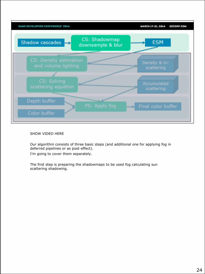
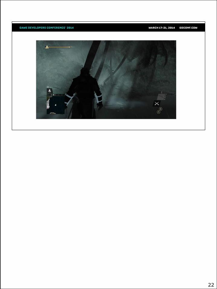
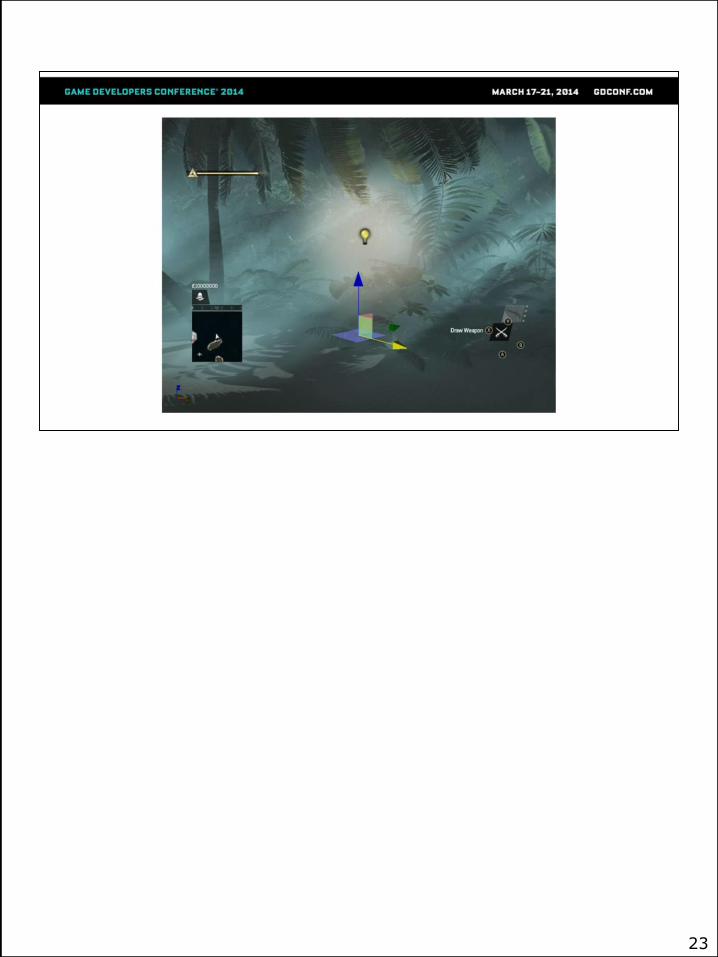
SHOW VIDEO HERE
Our algorithm consists of three basic steps (and additional one for applying fog in deferred pipelines or as post-effect).
I’m going to cover them separately.
The first step is preparing the shadowmaps to be used fog calculating sun scattering shadowing.
24
Why do we need it?
Our regular shadowing cascades were very high resolution (4 cascades, 1k x 1k) and had dense, high resolution information in them.
It was way too much detail for us, especially for close ranges and in first two cascades, condensed in first couple meters.
For smooth and approximate volumetric fog we needed something of much smaller resolution to reduce any flickering / aliasing artifacts from moving foliage etc.
First implementations using wide kernel PCF had very poor performance and still some flickering and aliasing artifacts.
25

The solution came from Exponential Shadow Maps algorithm.
First we downsample our cascaded shadowmaps four times (target R32F 1024 x 256 texture). During downsampling we calculate exponential shadowing probability distribution (see Exponential Shadow Mapping, an extension to Variance Shadow Mapping using exponential probabilistic distribution function instead of Chebyshevsinequality).
We also do additional separable box filter (as two separate steps) during this pass to make shadows softer and remove aliasing artifacts.
26

The solution came from Exponential Shadow Maps algorithm.
First we downsample our cascaded shadowmaps four times (target R32F 1024 x 256 texture). During downsampling we calculate exponential shadowing probability distribution (see Exponential Shadow Mapping, an extension to Variance Shadow Mapping using exponential probabilistic distribution function instead of Chebyshevsinequality).
We also do additional separable box filter (as two separate steps) during this pass to make shadows softer and remove aliasing artifacts.
27
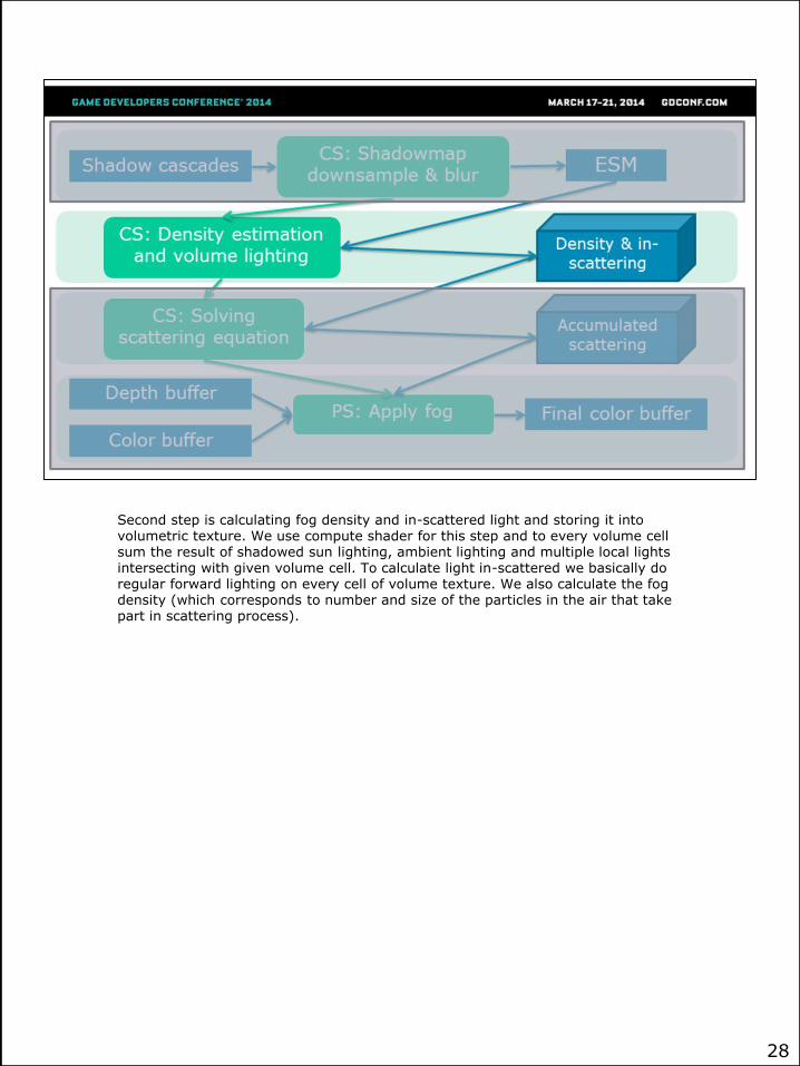
Second step is calculating fog density and in-scattered light and storing it into volumetric texture. We use compute shader for this step and to every volume cell sum the result of shadowed sun lighting, ambient lighting and multiple local lights intersecting with given volume cell. To calculate light in-scattered we basically do regular forward lighting on every cell of volume texture. We also calculate the fog density (which corresponds to number and size of the particles in the air that take part in scattering process).
28
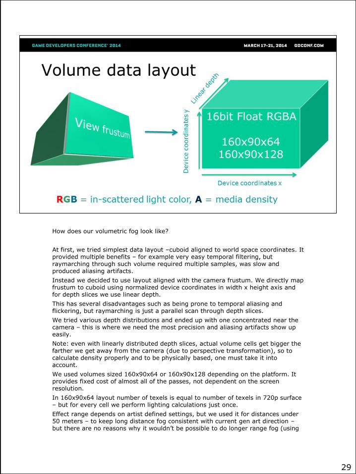
How does our volumetric fog look like?
At first, we tried simplest data layout –cuboid aligned to world space coordinates. It provided multiple benefits – for example very easy temporal filtering, but raymarching through such volume required multiple samples, was slow and produced aliasing artifacts.
Instead we decided to use layout aligned with the camera frustum. We directly map frustum to cuboid using normalized device coordinates in width x height axis and for depth slices we use linear depth.
This has several disadvantages such as being prone to temporal aliasing and flickering, but raymarching is just a parallel scan through depth slices.
We tried various depth distributions and ended up with one concentrated near the camera – this is where we need the most precision and aliasing artifacts show up easily.
Note: even with linearly distributed depth slices, actual volume cells get bigger the farther we get away from the camera (due to perspective transformation), so to calculate density properly and to be physically based, one must take it into account.
We used volumes sized 160x90x64 or 160x90x128 depending on the platform. It provides fixed cost of almost all of the passes, not dependent on the screen resolution.
In 160x90x64 layout number of texels is equal to number of texels in 720p surface – but for every cell we perform lighting calculations just once.
Effect range depends on artist defined settings, but we used it for distances under 50 meters – to keep long distance fog consistent with current gen art direction –but there are no reasons why it wouldn’t be possible to do longer range fog (using
29

exponential depth distribution or cascaded approach)
29

The resolution of our volume textures may seem extremely low, but it is sufficient:
1. We store low frequency information for every depth stored along the ray.
2. Every target pixel receives information about proper and precise depth from its native resolution.
3. Due to the fact that when applying effect, we use quadrilinear filtering on volumetric data, we are unable to see single texels of volume texture.
4. Perspective correction and volume shape makes sure that information is distributed correctly
Obviously, produced effect is very soft and is missing high frequency geometric details, but it fits our art direction and is quite similar to reality (because in the real atmosphere multiple scattering effect takes place and softens the look of light shafts a lot).
30

[!] In the first volumetric pass of the algorithm, we use compute shaders to build participating media lighting and its density.
Compute shaders are much easier to prototype that kind of effects due to possibility of use of 3D texture UAVs – we don’t need to set up geometry shader to target slices.
We combined density and lighting calculations due to a bit smaller bandwidth usage, but they can be split and totally decoupled.
This would allow to for example have volumes adding some media density locally to simulate smoke emission or have fully art driven fog layout. Another possibility would be to have optimization for lights – calculate it only inside volume, not in loop for every texel.
Density calculation is pretty straightforward, it is just one octave of Perlin noise that is animated by wind. We tried using multiple octaves, but in the end difference was rather subtle for added cost.
We also calculated vertical media density attenuation, as usually heavy particles such as steam water particles tend to gather around the ground level.
[!] For lighting part we simply accumulated lighting from main light (sun/moonlight), constant ambient term and multiple dynamic point lights that were intersecting with view frustum and marked by artists as lights affecting the atmosphere.
We used mentioned Exponential Shadow Maps shadowing technique to get shadows from the main light.
31

On AC4 we didn’t have any physically-based phase functions. Lighting color gradient (oriented towards direction of sun) was purely art-driven.
We had 2 colors of phase function – in direction of the sun and in opposite direction, apart from that with fully isotropic shape.
Obviously, any phase function can be applied in this pass to achieve more physically-correct effect.
32

1. Third step is solving the scattering equation by linearly marching through the fog volume and performing a numerical calculus solution.
2. Fourth step that is typical to deferred renderer is combining data from scattering solution (just one bilinear volume texture fetch!), depth buffer and lighting buffer without the fog. This step is not required in forward rendering pipelines.
33

So how do we solve this scattering equation?
The out-scattering effect is described by Beer-Lambert law, exponential falloff function of density integral for given distance.
For the in-scattering it is simple sum of in scattered lighting so far (taking distance based out scattering into account).
We have already our in-scattering values calculated and accumulated in the volume texture.
Therefore, for every ray we can simply march through the volume starting from camera, calculate the density sum, accumulate in-scattering radiance and out-scattering falloff factor.
(next slide)
34
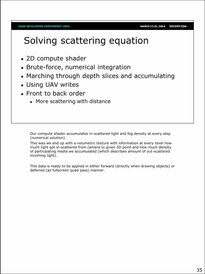
Our compute shader accumulates in-scattered light and fog density at every step (numerical solution).
This way we end up with a volumetric texture with information at every texel how much light got in-scattered from camera to given 3D point and how much density of participating media we accumulated (which describes amount of out-scattered incoming light).
This data is ready to be applied in either forward (directly when drawing objects) or deferred (as fullscreen quad pass) manner.
35

Our compute shader accumulates in-scattered light and fog density at every step (numerical solution).
This way we end up with a volumetric texture with information at every texel how much light got in-scattered from camera to given 3D point and how much density of participating media we accumulated (which describes amount of out-scattered incoming light).
This data is ready to be applied in either forward (directly when drawing objects) or deferred (as fullscreen quad pass) manner.
36
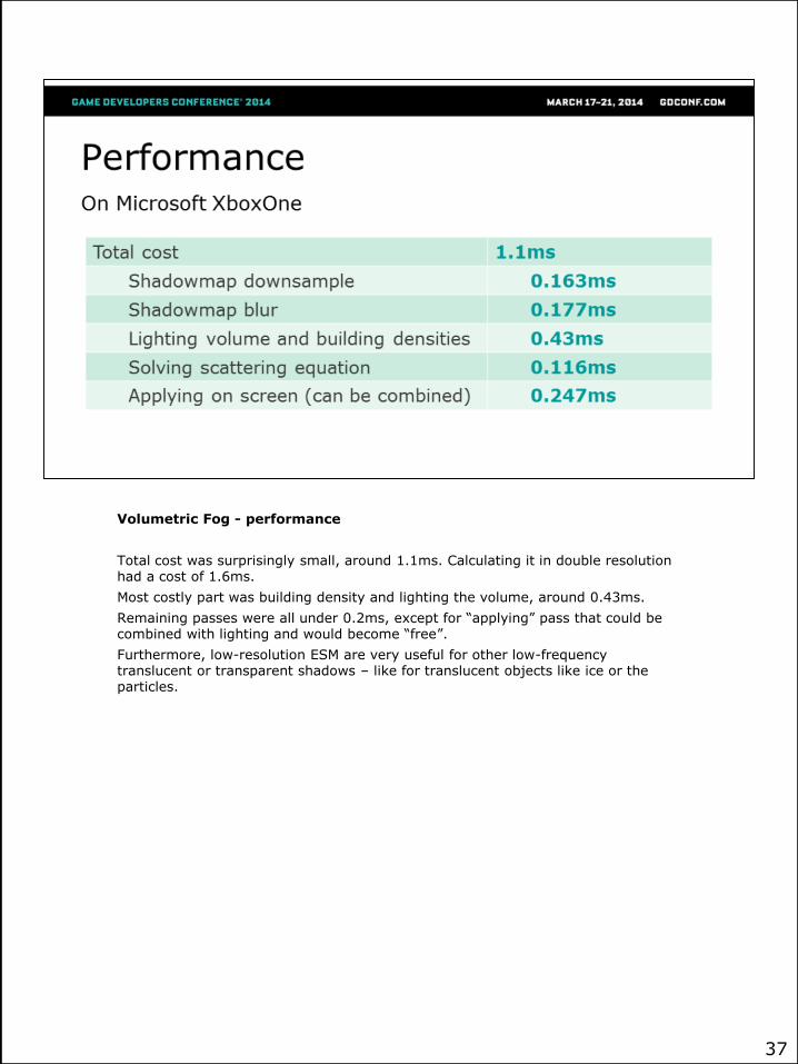
Volumetric Fog - performance
Total cost was surprisingly small, around 1.1ms. Calculating it in double resolution had a cost of 1.6ms.
Most costly part was building density and lighting the volume, around 0.43ms.
Remaining passes were all under 0.2ms, except for “applying” pass that could be combined with lighting and would become “free”.
Furthermore, low-resolution ESM are very useful for other low-frequency translucent or transparent shadows – like for translucent objects like ice or the particles.
37
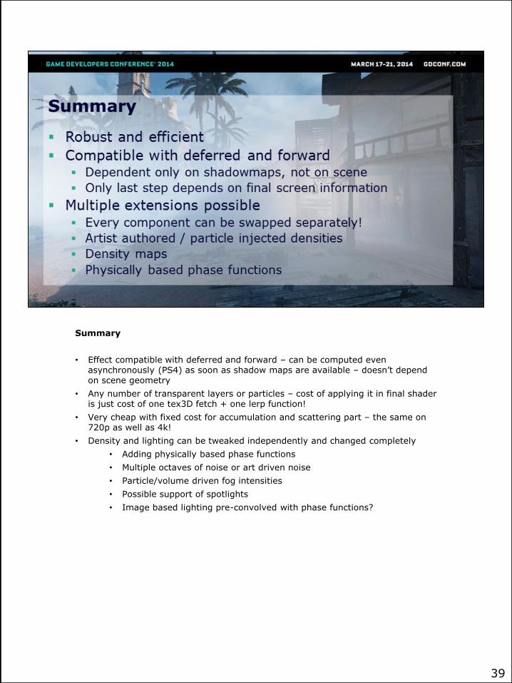
Summary
• Effect compatible with deferred and forward – can be computed even asynchronously (PS4) as soon as shadow maps are available – doesn’t depend on scene geometry
• Any number of transparent layers or particles – cost of applying it in final shader is just cost of one tex3D fetch + one lerp function!
• Very cheap with fixed cost for accumulation and scattering part – the same on 720p as well as 4k!
• Density and lighting can be tweaked independently and changed completely
• Adding physically based phase functions
• Multiple octaves of noise or art driven noise
• Particle/volume driven fog intensities
• Possible support of spotlights
• Image based lighting pre-convolved with phase functions?
38
Summary
• Effect compatible with deferred and forward – can be computed even asynchronously (PS4) as soon as shadow maps are available – doesn’t depend on scene geometry
• Any number of transparent layers or particles – cost of applying it in final shader is just cost of one tex3D fetch + one lerp function!
• Very cheap with fixed cost for accumulation and scattering part – the same on 720p as well as 4k!
• Density and lighting can be tweaked independently and changed completely
• Adding physically based phase functions
• Multiple octaves of noise or art driven noise
• Particle/volume driven fog intensities
• Possible support of spotlights
• Image based lighting pre-convolved with phase functions?
39
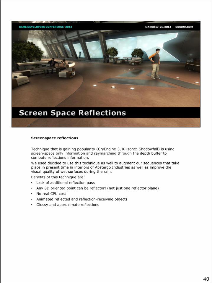
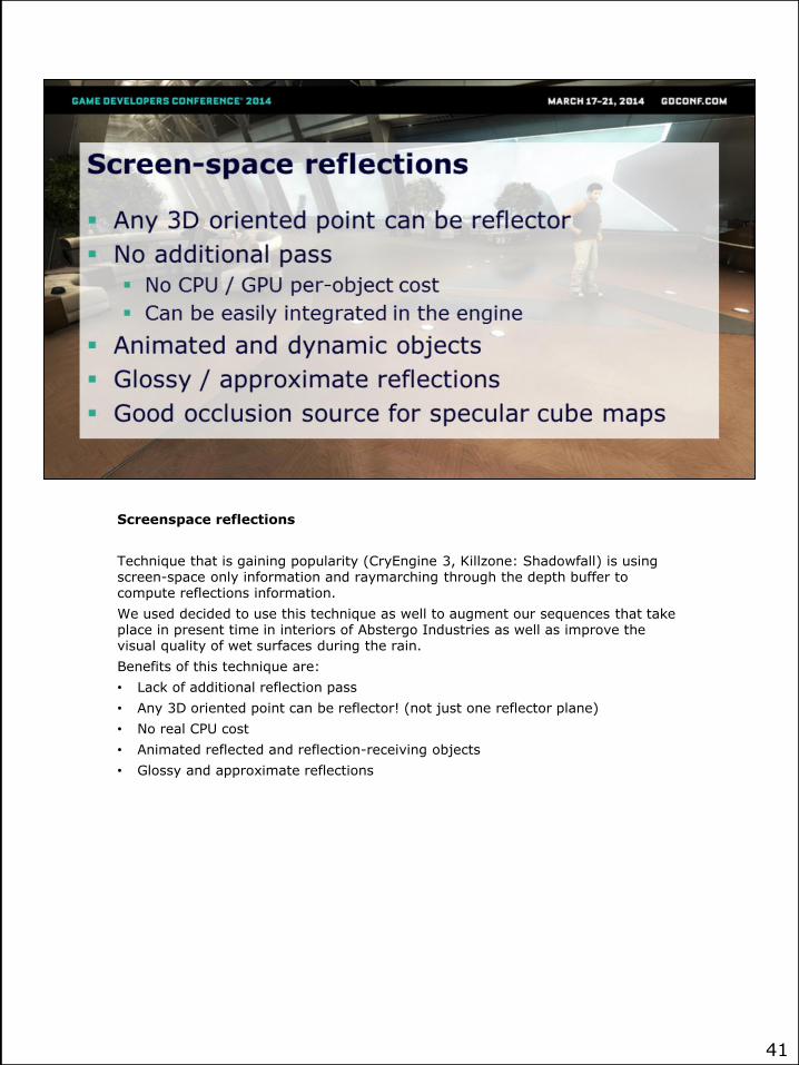
Screenspace reflections
Technique that is gaining popularity (CryEngine 3, Killzone: Shadowfall) is using screen-space only information and raymarching through the depth buffer to compute reflections information.
We used decided to use this technique as well to augment our sequences that take place in present time in interiors of Abstergo Industries as well as improve the visual quality of wet surfaces during the rain.
Benefits of this technique are:
• Lack of additional reflection pass
• Any 3D oriented point can be reflector! (not just one reflector plane)
• No real CPU cost
• Animated reflected and reflection-receiving objects
• Glossy and approximate reflections
40
Screenspace reflections
Technique that is gaining popularity (CryEngine 3, Killzone: Shadowfall) is using screen-space only information and raymarching through the depth buffer to compute reflections information.
We used decided to use this technique as well to augment our sequences that take place in present time in interiors of Abstergo Industries as well as improve the visual quality of wet surfaces during the rain.
Benefits of this technique are:
• Lack of additional reflection pass
• Any 3D oriented point can be reflector! (not just one reflector plane)
• No real CPU cost
• Animated reflected and reflection-receiving objects
• Glossy and approximate reflections
41

Without the screenspace reflections
42
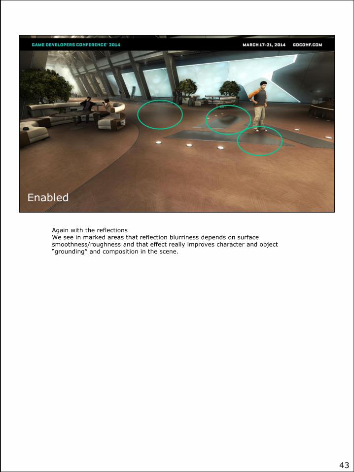
Again with the reflectionsWe see in marked areas that reflection blurriness depends on surface smoothness/roughness and that effect really improves character and object “grounding” and composition in the scene.
43
44
45
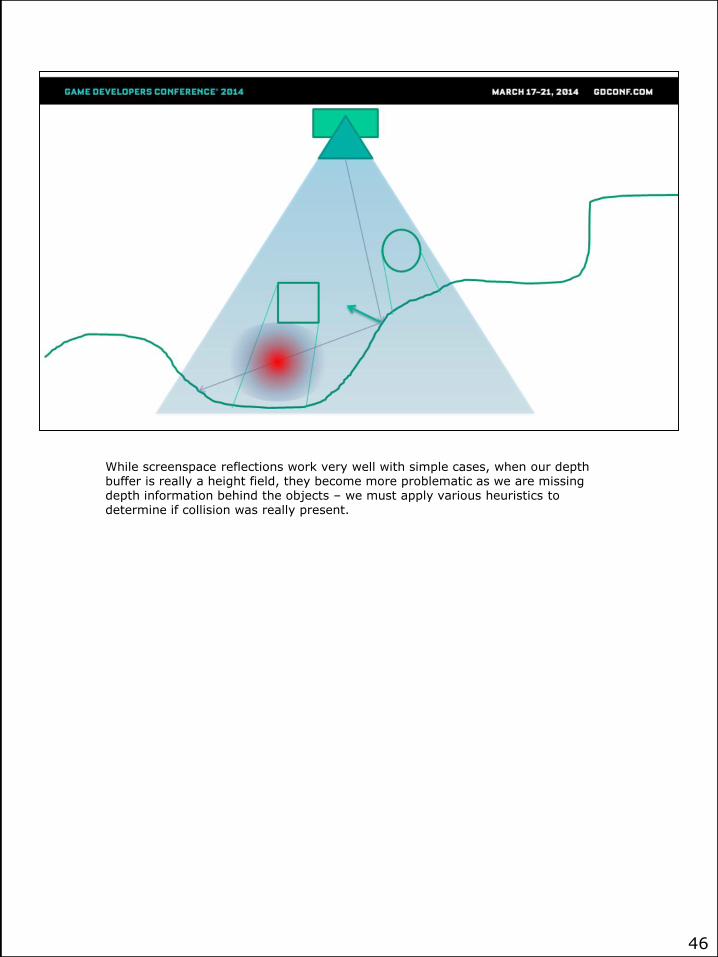
While screenspace reflections work very well with simple cases, when our depth buffer is really a height field, they become more problematic as we are missing depth information behind the objects – we must apply various heuristics to determine if collision was really present.
46
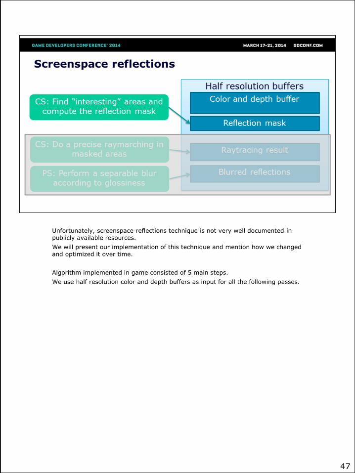
Unfortunately, screenspace reflections technique is not very well documented in publicly available resources.
We will present our implementation of this technique and mention how we changed and optimized it over time.
Algorithm implemented in game consisted of 5 main steps.
We use half resolution color and depth buffers as input for all the following passes.
47

Screenspace reflections can only sample valid, on-screen information. Usually amount of this information is limited and depending on scene glossiness and situation, the actual reflections would take 5-60% of the screen size.
Here we see potential reflections mask – only those pixels have chance to receive some reflections, rest of them do not have access to enough on-screen information or don’t have high glossiness / Fresnel factor for the reflections to be noticeable.
To calculate this mask and accelerate further raytracing, we calculated this mask.
For every 64x64 pixels block (of half resolution buffer) we were launching 64 low-precision rays. We used a pre-computed, non-uniform jittered distribution of ray positions to minimize the aliasing artifacts. Those rays were very fast – had large step and very high depth tolerance (both 4x larger than the final ones) and were used just to simply find if given surface reflects any on-screen information. This way subsequent passes that were more precise didn’t need to be launched for areas and surfaces that would reflect objects that are off-screen. To mark those areas we used UAV scatter write capability of compute shaders.
Notice that every ray covered a bit larger area than just its influence – this way we reduced temporal noise of the mask.
48
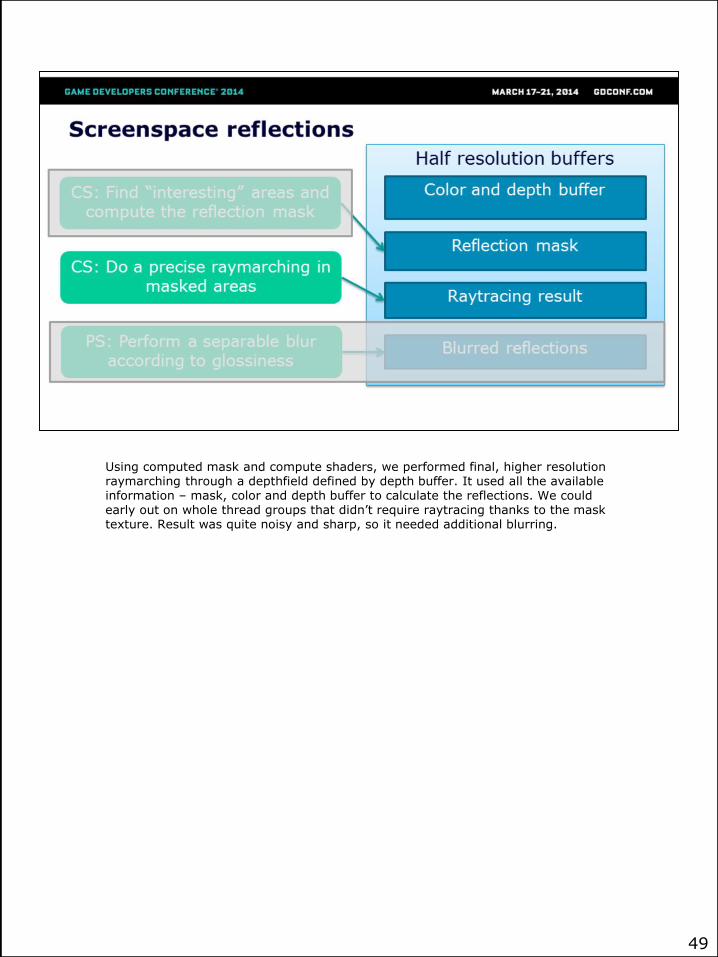
Using computed mask and compute shaders, we performed final, higher resolution raymarching through a depthfield defined by depth buffer. It used all the available information – mask, color and depth buffer to calculate the reflections. We could early out on whole thread groups that didn’t require raytracing thanks to the mask texture. Result was quite noisy and sharp, so it needed additional blurring.
49
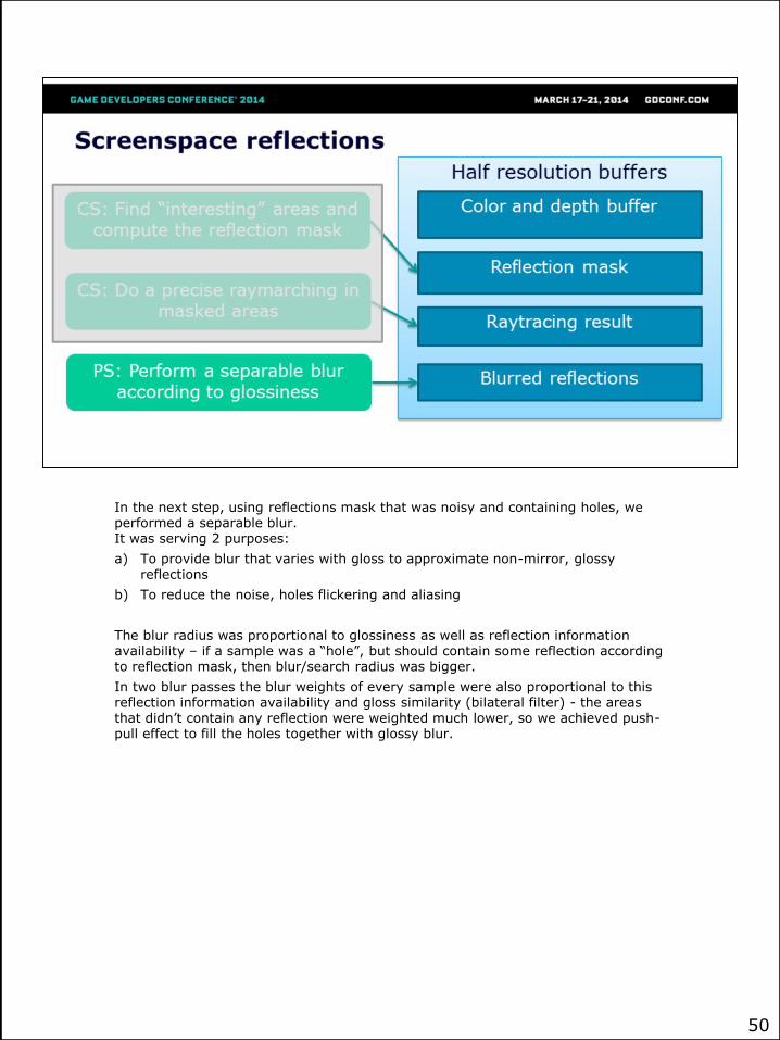
In the next step, using reflections mask that was noisy and containing holes, we performed a separable blur. It was serving 2 purposes:
a) To provide blur that varies with gloss to approximate non-mirror, glossy reflections
b) To reduce the noise, holes flickering and aliasing
The blur radius was proportional to glossiness as well as reflection information availability – if a sample was a “hole”, but should contain some reflection according to reflection mask, then blur/search radius was bigger.
In two blur passes the blur weights of every sample were also proportional to this reflection information availability and gloss similarity (bilateral filter) - the areas that didn’t contain any reflection were weighted much lower, so we achieved push-pull effect to fill the holes together with glossy blur.
50
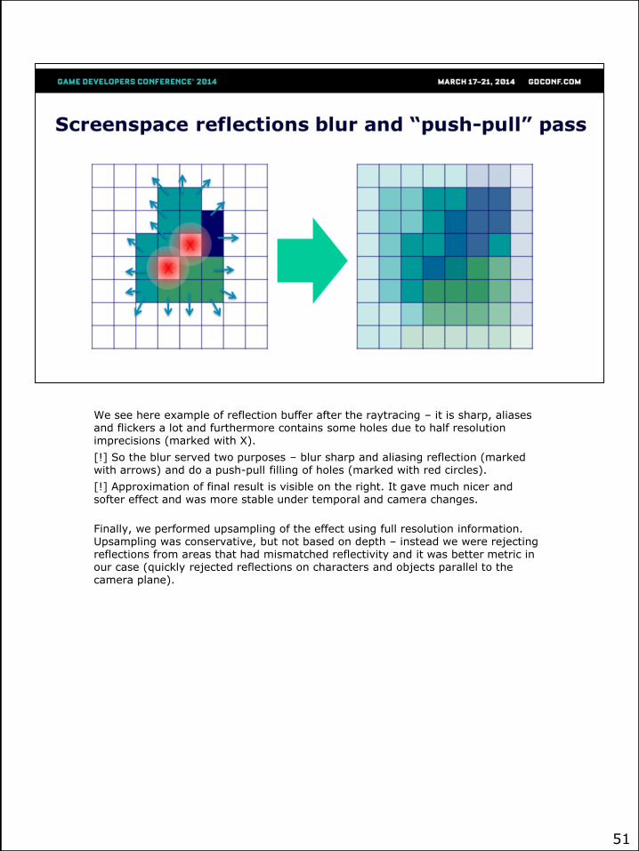
We see here example of reflection buffer after the raytracing – it is sharp, aliases and flickers a lot and furthermore contains some holes due to half resolution imprecisions (marked with X).
[!] So the blur served two purposes – blur sharp and aliasing reflection (marked with arrows) and do a push-pull filling of holes (marked with red circles).
[!] Approximation of final result is visible on the right. It gave much nicer and softer effect and was more stable under temporal and camera changes.
Finally, we performed upsampling of the effect using full resolution information. Upsampling was conservative, but not based on depth – instead we were rejecting reflections from areas that had mismatched reflectivity and it was better metric in our case (quickly rejected reflections on characters and objects parallel to the camera plane).
51

On totally reflective scene (glossy floor and objects – like on the screenshot on my previous slide) effect was costing us around 2ms on both next gen consoles.
On average scene (couple water puddles on screen in Havana) it was around 1ms.
Analysis of PIX capture shows that all of the passes timed between 0.1ms and 0.3ms.
52

53
54

Before I talk about the optimizations for the next gen consoles we have done, I wanted to discuss important architecture properties and differences that change approach to all optimizations.
Everyone who has done some GPU optimizations work for current-gen consoles –PS3 and X360 – knows that they are relatively easy.
To optimize timing, we simply:
• [!] Reduce amount of work for whole GPU by changing the algorithm and resolution (for example doing blur in half resolution).
• [!] Reduce the work done by shaders themself – by using less ALU instructions, precomputing some data and using look-up tables
• [!] Reduce used memory and bandwidth by doing less texture fetches (or more cache-friendly ones by keeping sample position coherency) and changing resource formats to ones using less memory
• [!] Finally, we can improve performance a lot (especially on PS3) by allowing proper instruction pipelining, reordering and micro optimizations – some instruction cost and latency can be perfectly hidden by other ones.
55
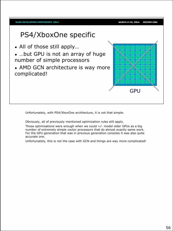
Unfortunately, with PS4/XboxOne architecture, it is not that simple.
Obviously, all of previously mentioned optimization rules still apply.
Those optimisations were enough when we could +/- model older GPUs as a big number of extremely simple vector processors that do almost exactly same work. For the GPU generation that was in previous generation consoles it was also quite accurate one.
Unfortunately, this is not the case with GCN and things are way more complicated!
56
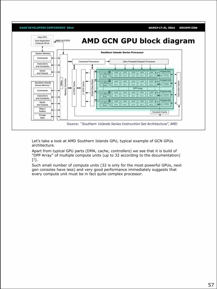
Let’s take a look at AMD Southern Islands GPU, typical example of GCN GPUs architecture.
Apart from typical GPU parts (DMA, cache, controllers) we see that it is build of “DPP Array” of multiple compute units (up to 32 according to the documentation) [!].
Such small number of compute units (32 is only for the most powerful GPUs, next gen consoles have less) and very good performance immediately suggests that every compute unit must be in fact quite complex processor.
57
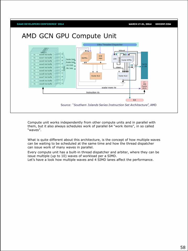
Compute unit works independently from other compute units and in parallel with them, but it also always schedules work of parallel 64 “work items”, in so called “waves”.
What is quite different about this architecture, is the concept of how multiple waves can be waiting to be scheduled at the same time and how the thread dispatcher can issue work of many waves in parallel.
Every compute unit has a built-in thread dispatcher and arbiter, where they can be issue multiple (up to 10) waves of workload per a SIMD. Let’s have a look how multiple waves and 4 SIMD lanes affect the performance.
58

59

60
Latency of memory operations is potentially huge – up to hundreds of cycles with a cache miss.
To hide it, you need to have much higher shader wave occupancy and proper ALU to memory operation ratio – so other waves can execute some work in the mean time.
With such code modifications, we can achieve almost perfect pipelining of multiple waves and great parallelism of costly memory operations.
61

Latency of memory operations is potentially huge – up to hundreds of cycles with a cache miss.
To hide it, you need to have much higher shader wave occupancy and proper ALU to memory operation ratio – so other waves can execute some work in the mean time.
With such code modifications, we can achieve almost perfect pipelining of multiple waves and great parallelism of costly memory operations.
But SIMD can execute up to 10 waves, what defines how many waves can be really scheduled and waiting for dispatch?
All waves active on the CU must share various resources.
So key factor to increasing wave occupancy is limiting the dependencies between work items and using less available resources.
62

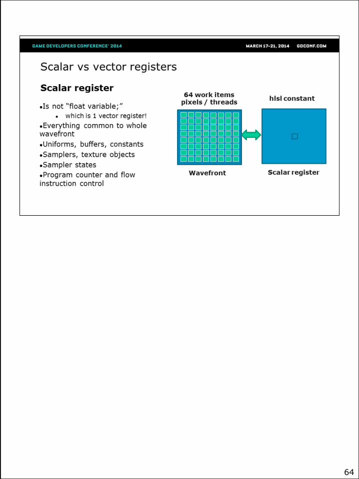
First, I wanted to talk about common misunderstanding on what is scalar and vector register.
63
64
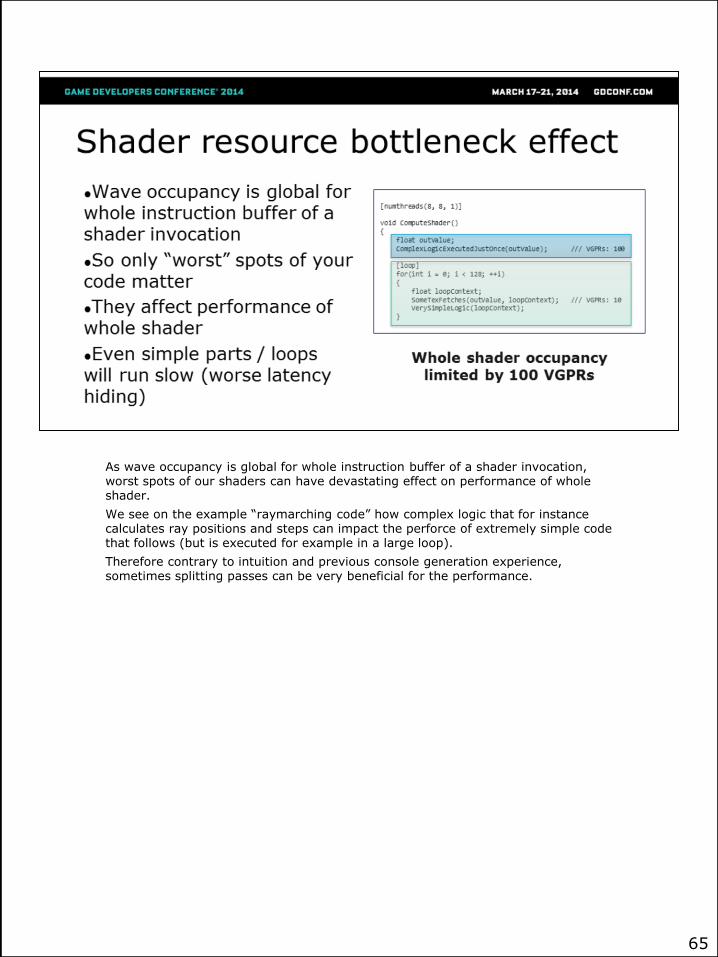
As wave occupancy is global for whole instruction buffer of a shader invocation, worst spots of our shaders can have devastating effect on performance of whole shader.
We see on the example “raymarching code” how complex logic that for instance calculates ray positions and steps can impact the perforce of extremely simple code that follows (but is executed for example in a large loop).
Therefore contrary to intuition and previous console generation experience, sometimes splitting passes can be very beneficial for the performance.
65
We were used to programming on current gen consoles, Microsoft Xbox 360 and Sony PlayStation 3, but with the next gen consoles that shader AMD Southern Islands architecture, some of common optimizations for those platforms turned out to be counter-productive and we observed benefits from other ones:
• We observed that crucial factor defining performance on the next gen consoles is Compute Unit shader wave occupancy. In almost all cases with both compute and pixel shaders we observed big performance differences.
• Only limiting factor on wave occupancy counts – so even halving down the number of vector registers won’t help if we are scalar register bound. Microsoft PIX for Xbox One has great tools to debug shaders and their register usage.
• Very easy way to minimize shader register usage is to minimize temporary shader variables lifetime
• Using old, DX9 sampler semantics will result in sub-optimal performance due to *multiple* fetched sampler states and muliple scalar registers they occupy. Re-use the sampler states and minimize their number.
• This can be especially tricky for ports from DX9 engines that use old combined sampler/texture object semantics. This can degrade your performance.
• Often it is better to use Load or operator[] intrinsic for sampling instead of Sample – especially for compute shaders and post effects where sampling position is precise and known. Load uses less scalar registers and it can increase your wave occupancy. Be careful though with half pixel offsets and rounding when converting from floats!
66

• Usually to save bandwidth (especially on X360 where “resolve” operation had non-negligible costs) and achieve better pixel shader texture cache latency hiding we were combining multiple passes together. Using compute shaders it is even easier – using local memory and thread synchronization multiple passes can be batched together. We were surprised to find out that very often, such attempts are counter-productive.
• Another example is that changing from 16 taps PCF done in CS to separable filtered ESM provided nice gains of performance and quality.
• Local Data Storage memory is very fast and convenient, but using too much of it (especially in “big” thread groups) tends to break down parallelism.
67

68
• It is sometimes better to loop and branch, than to unroll. Shader compiler can bump up register usage for an unrolled loop and it can cause worse performance. Branches increase register usage as well, so should be used sparingly, but if one of shader branches means no work and you can provide good PS quad or CS warp group coherency, they are beneficial to skip lots of ALU and memory reads.
• We saw best performance and shader code with partially and manually unrolled loops (for example operating on 4 samples at the same time). For some reason shader compilers don’t do such good job with [unroll] …
• Vector registers and instructions operate on single components of float4 so if you don’t need 4 components in your calculations, don’t do it! This way thread dispatcher will be able to schedule some other work on freed lane. Common situation is storing color in float4 – which is not always necessary.
• This one is pretty obvious, but in shader model 4.0-5.0 there are tons on new cool instructions! If you just got to next gen development from PS3/X360, read the documentation and find the ones useful for you.
69

70
71

72

73

74

75
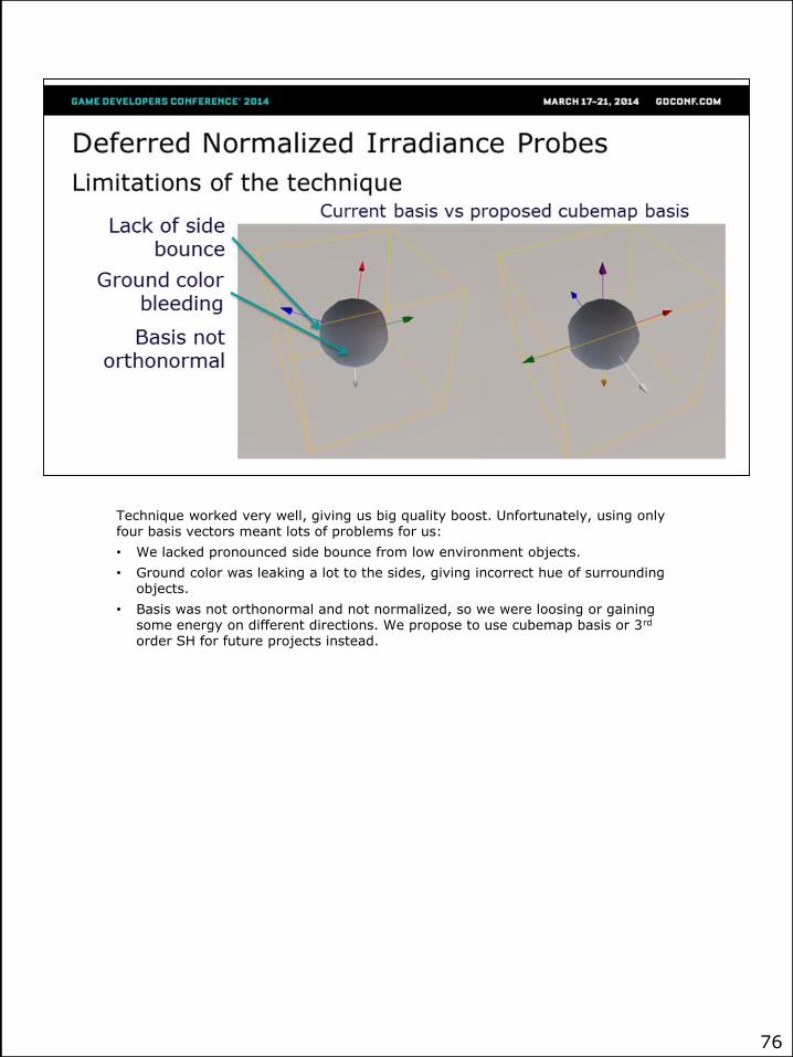
Technique worked very well, giving us big quality boost. Unfortunately, using only four basis vectors meant lots of problems for us:
• We lacked pronounced side bounce from low environment objects.
• Ground color was leaking a lot to the sides, giving incorrect hue of surrounding objects.
• Basis was not orthonormal and not normalized, so we were loosing or gaining some energy on different directions. We propose to use cubemap basis or 3rd
order SH for future projects instead.
76

We know about multiple limitations of our technique – most of them come from requirement of consistent art direction of current gen and next gen versions –artists and lighters didn’t want to duplicate their whole work and we wanted to avoid platform-specific content bugs.
1. We wanted to change irradiance storage basis to something more accurate and physically based. HL2 basis with added “wrap-around” vector pointing down didn’t work very well. It is also not orthonormal basis, we either add or lose energy and we lose lots of detail on sides. We have tried cubemap basis (6 basis vectors) and it gave definitely superior results, but had to drop it due to either mismatch between current gen/next gen or performance cost on the current gen. Conclusion: use cubemap basis or SH basis (3rd order may not be the best to store PRT, but seems perfect for storing the irradiance).
2. We thought about adding some indirect specular on shiny objects. First attempts were promising, but had to drop it due to doubling evaluation cost on the current gen.
3. Increase probe density. This one is pretty straightforward, on the next gen we could have much higher probe density. We could also have multiple layers in height axis instead of blending it out with height – it would work perfectly with AC level layout even with just couple layers.
4. Instead of storing “normalized” irradiance, we could store real, HDR irradiance together with indirect sky lighting. We dropped it due to current gen memory cost (multiple weather presets).
5. Handle multiple bounces. This is yet another feature we had working, but dropped it due to increased baking time and the lack of HDR.
6. Update some probes – for example close ones – in the real time (distributed between couple frames). Definitely possible on the next gen consoles
77

(especially that we store everything on the GPU) and indirect lighting would have shadowing information from dynamic objects as well.
77

78
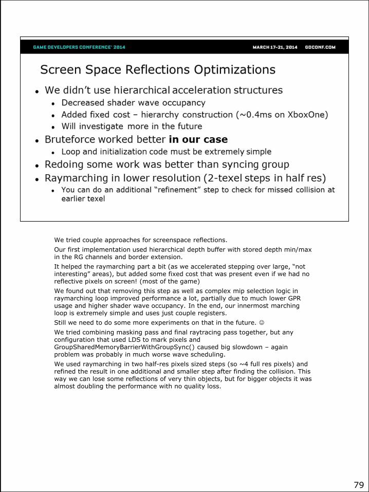
We tried couple approaches for screenspace reflections.
Our first implementation used hierarchical depth buffer with stored depth min/max in the RG channels and border extension.
It helped the raymarching part a bit (as we accelerated stepping over large, “not interesting” areas), but added some fixed cost that was present even if we had no reflective pixels on screen! (most of the game)
We found out that removing this step as well as complex mip selection logic in raymarching loop improved performance a lot, partially due to much lower GPR usage and higher shader wave occupancy. In the end, our innermost marching loop is extremely simple and uses just couple registers.
Still we need to do some more experiments on that in the future.
We tried combining masking pass and final raytracing pass together, but any configuration that used LDS to mark pixels and GroupSharedMemoryBarrierWithGroupSync() caused big slowdown – again problem was probably in much worse wave scheduling.
We used raymarching in two half-res pixels sized steps (so ~4 full res pixels) and refined the result in one additional and smaller step after finding the collision. This way we can lose some reflections of very thin objects, but for bigger objects it was almost doubling the performance with no quality loss.
79
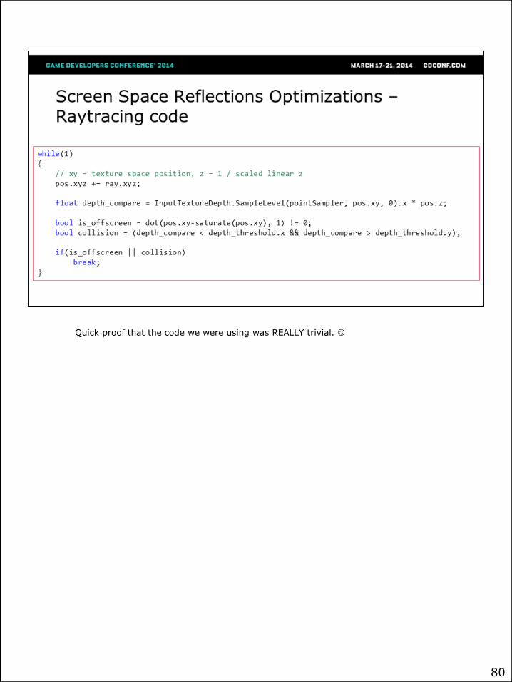
Quick proof that the code we were using was REALLY trivial.
80

Parallax Occlusion Mapping
We were interested in increasing geometric detail on objects, but after some prototypes done on tesselation in the company we knew that tesselation means completely different content pipeline, problems with geometric discontinuities, lack of smoothing groups, UV seams etc.
We didn’t want to go this way, especially that only few artists were creating next-gen specific content.
We wanted to have a solution that could be applied easily on existing current-gen assets and increase their perceived geometric detail, on all mesh types and just by switching material and creating a new heightmap texture – under such constraints parallax occlusion mapping seemed like a perfect fit for us.
We found it working really nice especially with some layered materials – it gave really interesting look on for example moss on stones.
Only one layer has parallax occlusion mapping – which gives really volumetric impression of one layer on top of the other without the need to draw two meshes, use decals or alpha blended objects.
We were aware of multiple artifacts on mesh corners, UV seams etc. but in final game we didn’t see them due to subtleness of the effect. Still, it improved perceived depth when for example climbing rock walls.
Bruteforce approach worked really well for us after some code micro-optimizations. In general, we didn’t see any performance impact on typical scenes.
We tried “Quadtree Displacement Mapping” by Michal Drobot, but saw no performance difference (lower wave occupancy?).
81

On POM just like on screenspace reflections, brute-force linear search worked very well. We tried quadtree displacement mapping, but it was giving similar performance and quality results – due to much lower shader wave occupancy, so we kept simpler solution with less asset dependency.
To get smooth effect without problems at grazing angles and without aliasing and performance problems in distance, it is quite important to pre-calculate mip level and fade the effect out manually with distance.
It is beneficial to batch up to four reads together on PS4 (see Valient, “KillzoneShadowfall Demo Postmortem”, Guerilla Games) and *in this case* partially unroll the loops.
Remember to turn off aniso filtering on height maps and similar textures! In our engine texture filtering of asset textures is artist driven and at first they didn’t set it for heightmap textures…
82

Whole “bruteforce” Parallax Occlusion Mapping algorithm – how we batch texture reads together.
Note that:
• There is safety guard (24 iterations) added mainly for the game editor – to avoid driver crash when for example mesh with wrong tangent space is provided.
• Miplevel is calculated just once and assumed constant
• In branch coordinates are checked in reverse order (we effectively pick the closest hit)
83

Rain
Tropical climate of Caribbean Sea area is extremely unpredictable with often rain showers and rain storms.
We had a decent weather system used in previous AC games, but we wanted to improve overall look of rain and wet surfaces.
On the next gen consoles, we wanted to use compute and geometry shaders to achieve this effect and have fully procedural, but art-driven effect.
SHOW VIDEO HERE
84
Rain drop system – simulation and rendering
Due to rather simple nature of rain simulation (but massive particle count), we decided to keep whole simulation on GPU.
Rain behavior and physics were simulated using compute shaders and then later expanded from points to target rain geometry using geometry shaders.
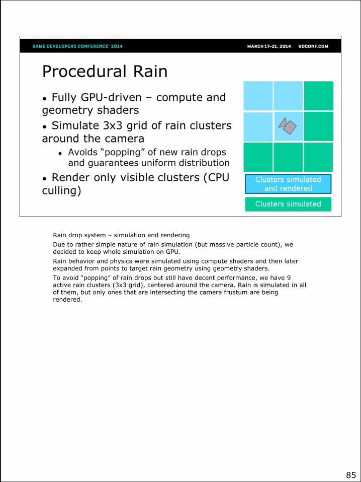
To avoid “popping” of rain drops but still have decent performance, we have 9 active rain clusters (3x3 grid), centered around the camera. Rain is simulated in all of them, but only ones that are intersecting the camera frustum are being rendered.
85
We take multiple factors into account during the simulation
86
Rain update process:
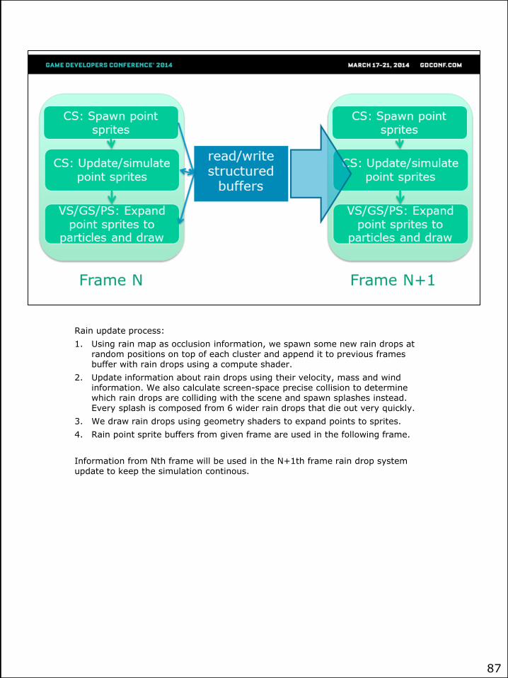
1. Using rain map as occlusion information, we spawn some new rain drops at random positions on top of each cluster and append it to previous frames buffer with rain drops using a compute shader.
2. Update information about rain drops using their velocity, mass and wind information. We also calculate screen-space precise collision to determine which rain drops are colliding with the scene and spawn splashes instead. Every splash is composed from 6 wider rain drops that die out very quickly.
3. We draw rain drops using geometry shaders to expand points to sprites.
4. Rain point sprite buffers from given frame are used in the following frame.
Information from Nth frame will be used in the N+1th frame rain drop system update to keep the simulation continous.
87
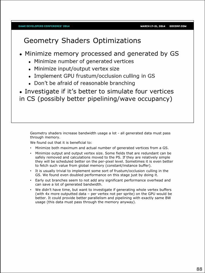
Geometry shaders increase bandwidth usage a lot - all generated data must pass through memory.
We found out that it is beneficial to:
• Minimize both maximum and actual number of generated vertices from a GS.
• Minimize output and output vertex size. Some fields that are redundant can be safely removed and calculations moved to the PS. If they are relatively simple they will be scheduled better on the per-pixel level. Sometimes it is even better to fetch such value from global memory (constant/instance buffer).
• It is usually trivial to implement some sort of frustum/occlusion culling in the GS. We found even doubled performance on this stage just by doing it.
• Early out branches seem to not add any significant performance overhead and can save a lot of generated bandwidth.
• We didn’t have time, but want to investigate if generating whole vertex buffers (with 4x more outputted data – per vertex not per sprite) on the GPU would be better. It could provide better parallelism and pipelining with exactly same BW usage (this data must pass through the memory anyway).
88
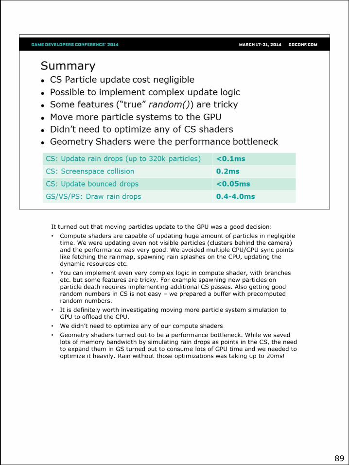
It turned out that moving particles update to the GPU was a good decision:
• Compute shaders are capable of updating huge amount of particles in negligible time. We were updating even not visible particles (clusters behind the camera) and the performance was very good. We avoided multiple CPU/GPU sync points like fetching the rainmap, spawning rain splashes on the CPU, updating the dynamic resources etc.
• You can implement even very complex logic in compute shader, with branches etc. but some features are tricky. For example spawning new particles on particle death requires implementing additional CS passes. Also getting good random numbers in CS is not easy – we prepared a buffer with precomputedrandom numbers.
• It is definitely worth investigating moving more particle system simulation to GPU to offload the CPU.
• We didn’t need to optimize any of our compute shaders
• Geometry shaders turned out to be a performance bottleneck. While we saved lots of memory bandwidth by simulating rain drops as points in the CS, the need to expand them in GS turned out to consume lots of GPU time and we needed to optimize it heavily. Rain without those optimizations was taking up to 20ms!
89

90

91