This is the peer reviewed version of the following article: “Vidal, T., Crainic, T. G., Gendreau, M., & Prins, C.

(2015). Timing problems and algorithms: Time decisions for sequences of activities. Networks, 65(2), 102–128”,

which has been published in final form at https://doi.org/10.1002/net.21587. It is also the final version of

the technical report named “A unifying view on timing problems and algorithms”. This article may be used for

non-commercial purposes in accordance with Wiley Terms and Conditions for Self-Archiving.

Timing problems and algorithms:

Time decisions for sequences of activities

Thibaut Vidal*CIRRELT & Departement d’informatique et de recherche operationnelle,

Universite de Montreal, Canada& ICD-LOSI, Universite de Technologie de Troyes, France

Thibaut.Vidal@cirrelt.ca

Teodor Gabriel CrainicCIRRELT & Departement de management et technologie, Ecole des sciences de la gestion, UQAM,

Montreal, Canada

Michel GendreauCIRRELT & Departement de mathematiques et genie industriel,

Ecole Polytechnique, Montreal, Canada

Christian PrinsICD-LOSI, Universite de Technologie de Troyes, France

Abstract

Timing problems involve the choice of task execution dates within a predetermined processing se-quence, and under various additional constraints or objectives such as time windows, time-dependentcosts, or flexible processing times, among others. Their efficient resolution is critical in branch andbound and neighborhood search methods for vehicle routing, project and machine scheduling, as wellas in various applications in network optimization, resource allocation and statistical inference. Timingrelated problems have been studied for years, yet research on this subject suffers from a lack of consen-sus, and most knowledge is scattered among operations research and applied mathematics domains.This article introduces a classification of timing problems and features, as well as a unifying multi-disciplinary analysis of timing algorithms. In relation to frequent application cases within branchingschemes or neighborhood searches, the efficient resolution of series of similar timing subproblems is alsoanalyzed. A dedicated formalism of re-optimization “by concatenation” is introduced to that extent.The knowledge developed through this analysis is valuable for modeling and algorithmic design, fora wide range of combinatorial optimization problems with time characteristics, including rich vehiclerouting settings and emerging non-regular scheduling applications, among others.

Keywords: Optimization, Timing, Scheduling, Routing, Resource allocation, Statistical inference,Branch and bound, Neighborhood search.

* Corresponding author

1

1 Introduction

Time-related constraints and objectives appear in a variety of flavors within scheduling, project man-agement, data transmission, routing, network optimization and numerous other fields. The relatedcombinatorial optimization problems, e.g. vehicle routing or machine scheduling, often require thearrangement of activities under time requirements, such as tasks, visits to customers, production ofobjects, and so on. Several combined decisions are required: the allocation of resources to activities,activities sequencing, and finally the adjustment – timing – of activity execution dates, speed and idletime, within the chosen sequence. To solve these combinatorial optimization problems, most heuristicand exact approaches perform a search through a large number of sequence and resource allocationalternatives, and use repeatedly a timing algorithm to produce adequate execution dates, filter fea-sible solutions and evaluate costs. The timing solution method is thus called extensively, such thatits complexity impacts dramatically the performance of the solution method, potentially making thedifference between successful algorithmic approaches and failure.

Timing algorithms are the cornerstone of complex algorithms for difficult combinatorial optimiza-tion problems, but the literature dedicated to this subject remains is scarce and scattered. In fact,most developments on timing are inherent to a specific field, such as project planning, shortest path,routing, scheduling, and statistical inference, which bring into play, quite unexpectedly, the same for-mulations. Few relationships between domains have been actually exploited and, thus, close conceptsand solution methods are independently developed within different formalisms, being rarely assessed ina more general context. In addition, real-life settings bring forth a large number of challenging timingvariants with different constraints and objectives, such as target execution dates, penalized idle time,(possibly multiple) time windows on activities, penalized lateness and earliness, speed decisions, time-dependent activity durations and costs, congestion, learning issues, and so on. Even if efficient timingalgorithms have been designed for some of these characteristics taken separately, problems involvingcombinations of characteristics become much more complex, and there is generally no systematic wayto extend concepts developed for the separate problems into a methodology for the new ones.

To address these challenges, this paper contributes to the timing field, by means of a multidisci-plinary review and analysis of timing features, problems, and algorithmic approaches. A large assort-ment of problems, often treated independently in the literature under various names, are identified andclassified in relation to their structure. Successful solution methods and solving concepts are invento-ried and analyzed. In the most noticeable cases, this analysis led to identify more than 26 algorithmsfrom different research fields as similar implementations of three main general approaches. Not onlydoes this review gather the keys for a stand-alone resolution of a large variety of timing problems, butit also analyzes the efficient resolution of timing problems within the context of global search methods,e.g. neighborhood-based heuristics and branch-and-bound-based approaches for rich vehicle routingand scheduling problems. For these applications, managing global information through the successiveresolution of similar timing instances can lead to dramatic reductions of the overall computationaleffort. To this extent, a re-optimization framework is introduced in the second part of this paper. Thebody of knowledge developed in this paper is critical for both modeling work and algorithmic design,enabling to point out relationships between problems and their respective complexities. A portfolio ofstate-of-the-art timing algorithms is identified, which will prove useful to build more generalist solversfor many variants of difficult combinatorial optimization problems. To our knowledge, no such unifyingreview and methodological analysis of this rich body of issues has been performed in the past.

The remainder of this paper is organized as follows: Section 2 formally defines timing problems,while Section 3 presents examples of applications. Section 4 provides a detailed classification of themain timing features encountered in the literature as well as notations. Our methodological analysisof timing problems and their independent resolution is then organized in Sections 5 and 6 relatively tothe previous classification. Section 7 finally introduces a re-optimization framework that encompasses

state-of-the-art approaches for solving series of related timing instances. Section 8 highlights a numberof challenging avenues of research in the timing field and presents the conclusions of this paper.

2 Problem statement

In this paper, the term activities is used to represent, independently of the field of application, ele-mentary operations that must be managed. The term date always stands for a point in time, whereasthe words duration or time are employed for relative values (e.g., processing time). Without loss ofgenerality, objective minimization is considered. The notation a+ stands for maxa, 0.

Definition 1 (General timing problem). Let A = (a1, . . . , an) be a sequence of n activities withprocessing times p1, . . . , pn. The execution dates of these activities t = (t1, . . . , tn) are required to followa total order with respect to the subscripts, such that ti + pi ≤ ti+1 for i ∈ 1, . . . , n-1. Additionalproblem features F x, for x ∈ 1, . . . ,m, provide the means to address particular settings with eithera role as objective, F x ∈ Fobj, or as constraint F x ∈ Fcons. Any feature F x is characterized by aset of mx functions fxy (t) for y ∈ 1, . . . ,mx. The general timing problem aims to find a feasibletiming solution t, respecting order constraints (Equation 2), features constraints (Equation 3), andminimizing the weighted sum of contributions from all feature objectives (Equation 1).

mint=(t1,...,tn)∈<n+

∑Fx∈Fobj

αx∑

1≤y≤mx

fxy (t) (1)

s.t. ti + pi ≤ ti+1 1 ≤ i < n (2)

fxy (t) ≤ 0 F x ∈ Fcons , 1 ≤ y ≤ mx (3)

The feature deadlines D, for example, involves a latest execution date di for each activity i, andcharacteristic functions fDi (t) = (ti − di)+ for i ∈ 1, . . . , n. When D takes the role of a constraint,fDi (t) = (ti−di)+ ≤ 0⇔ ti ≤ di yields the standard formulation of deadlines, while a role as objectiveleads to standard tardiness optimization criteria.

Timing problems can be viewed as shifting activity execution dates on a single resource, intro-ducing idle time and optimizing activity speed, depending upon the features, without changing theprocessing order. Most basic versions of timing are simple to address, while various features arisingfrom application cases can lead to dramatic increases in problem difficulty. It must also be notedthat features have been defined independently from their role as constraint or objective for two mainreasons. First, many algorithms are concerned with the effective calculation of some quantities, liketotal duration for example, which enables related constraints or objectives to be tackled in the sameway. Secondly, since constraints can be transformed into objectives by Lagrangian relaxation, it issometimes artificial to discriminate problems involving a given feature either as constraint or objective.Our study will thus be targeted on features, independently of their role, the latter being specified onlywhen relevant to the method. Finally, in the scheduling domain, some constraints and objectives, suchas due dates, are based on activity completion dates Ci = ti + pi. Without loss of generality, theseproblems are reformulated to involve only execution dates.

To emphasize the relations with practical problem settings, Section 3 details major problems inthe fields of operations research and applied mathematics leading to underlying timing structures.

3 Timing issues and major application fields

Production and project scheduling. The development of just-in-time policies leads to challengingnon-regular scheduling settings for which earliness or idle times are a major concern. In the earlinessand tardiness (E/T) scheduling problem, a sequence of activities (a1, . . . , an) is given with target

2

execution dates di and processing times pi, as well as penalty factors for earliness εi and tardinessτi. The goal is to determine the sequence of activities and their execution dates on a single machine,such that linear penalties incurred for early or late processing are minimized. This scheduling problemis NP-hard in the strong sense [60] and most recent resolution methods consider branch and bound,neighborhood search or other metaheuristic frameworks working on the activity sequence [5]. For everysequence explored during the search, a timing algorithm is applied to compute the activity executiondates and thus the sequence cost. The related problem is formulated in Equations (4-5).

min(t1,...,tn)∈<n+

n∑i=1

εi(di − ti)+ + τi(ti − di)+ (4)

s.t. ti + pi ≤ ti+1 1 ≤ i < n (5)

This timing problem is known to be solvable in O(n log n) (Sections 5.3 and 5.4). Yet, as thetiming resolution is the main bottleneck for most (E/T) scheduling approaches, extensive research hasbeen conducted to solve series of timing instances more efficiently within neighborhood searches. Theuse of global information through the search leads to timing “re-optimization” procedures working inamortized O(log n) complexity, and even O(1) for some particular cases, as described in Section 7.

Network optimization and vehicle routing. Timing subproblems are also frequently encounteredin network optimization settings, e.g., resource-constrained shortest paths, delivery-man and minimumlatency, vehicle routing and scheduling [40, 42, 146]. Thus, for example, the vehicle routing problemwith time windows (VRPTW) consists in designing vehicle itineraries to service a set of geographicallyscattered customers within allowed time intervals. This problem has been the focus of a significantresearch effort focused for a large part on heuristic methods [18, 19, 61]. In particular, it is commonto consider solutions with penalized time-constraint violations to enhance the search [148]. Differentrelaxation schemes can be applied, with lateness (Taillard et al. [140]), lateness and earliness (Ibarakiet al. [86, 87]), “returns in time” (Nagata et al. [109]), or speed-increase (Vidal et al. [148]), leading todifferent timing sub-problems for producing route schedules and evaluating penalties. Yet, the efficientresolution of these sub-problems is critical, since it determines the complexity of the neighborhood-search procedures, which are the bottleneck of many current metaheuristics.

One also observes a recent important focus on “richer” VRPs [68, 146], which explicitly takeinto account various combined constraints and objectives issued from application cases. These com-plex combinatorial optimization problems frequently involve temporal considerations, time-dependenttravel speed, crew costs, customer requirements in terms of visit times, employee breaks and dutytimes, learning or fatigue effects, fair repartition of working time among employees, and so on. Suchcharacteristics must be directly managed within route evaluations in heuristics and exact methods,thus leading to a large variety of timing subproblems.

Energy optimization. Norstad et al. [111] introduce a ship routing problem with convex speedoptimization, which presents two interlaced issues: the design of a ship itinerary, and the optimizationof arrival dates and speed to reduce fuel consumption. For a fixed sequence of visits, the lattersubproblem is formulated in Equations (6-9).

mint,v

n−1∑i=1

di,i+1 c(vi,i+1) (6)

s.t. ti + pi + di,i+1/vi,i+1 ≤ ti+1 1 ≤ i ≤ n− 1 (7)

ri ≤ ti ≤ di 1 ≤ i ≤ n (8)

vmin ≤ vi,i+1 ≤ vmax 1 ≤ i ≤ n− 1 (9)

3

The decision variables are the travel speeds vi,i+1 for i ∈ 1, . . . , n − 1 for each port-to-port leg,and the arrival dates at ports ti for i ∈ 1, . . . , n. The objective is to minimize the fuel consumptionon all trips, while respecting time-window constraints [ri, di] on arrival dates, and maintaining thespeed in a feasible range [vmin, vmax]. The convex function c(v) describes the energy consumption permile as a function of speed. Let vopt be the minimum of c(v), let di,i+1 represent the leg distancesand pi stand for processing times at ports. Equations (7-9) ensure that port arrival and departuredates are consistent with leg speeds, that time windows at port arrivals are respected, and finally thatspeeds are within a feasible range.

This problem can be reformulated to rely exclusively on arrival dates by defining an extendedcost/speed function c(v), which accounts for the fact that waiting times can be used in case of sub-optimal low speed values (Equations 10-13).

mint

n−1∑i=1

di,i+1c

(di,i+1

ti+1 − ti

)(10)

s.t. ti + pi +di,i+1

vmax≤ ti+1 1 ≤ i ≤ n− 1 (11)

ri ≤ ti ≤ di 1 ≤ i ≤ n (12)

with c(v) =

c(vopt) if v ≤ voptc(v) otherwise

(13)

The latter model falls into the category of timing problems. It involves time-window featurescharacterized by functions fi(t) = (ti − di)+ + (ri − ti)+ with a role as constraints, as well as flexibleprocessing times characterized by convex functions fi(t) = ci(ti+1 − ti) in the objective, such thatci(∆ti) = di,i+1c(di,i+1/∆ti). Hvattum et al. [84] and Norstad et al. [111] introduced a strongly poly-nomial Recursive Smoothing Algorithm (RSA) to solve the previous timing problem with a worst casecomplexity of O(n2). A similar algorithm was then used in the context of a vehicle routing problemwith CO2 minimization (Demir et al. [36]). Other timing algorithms and re-optimization proceduresare known for these settings (Sections 6.3 and 7.5.5).

Statistical Inference. The isotonic regression problem under a total order (IRC) constitutes anintensively studied particular case of our models. Given a vector N = (N1, . . . , Nn) of n real numbers,IRC seeks a vector of non-decreasing values t = (t1, . . . , tn) as close as possible to N according to adistance metric ‖ ‖ (generally the Euclidean distance), as in Equations (14-15).

mint=(t1,...,tn)

‖t−N‖ (14)

s.t. ti ≤ ti+1 1 ≤ i < n (15)

As underlined by the seminal books of Barlow et al. [8] and Robertson et al. [126], IRC is the keyto performing many restricted maximum likelihood estimates in statistics, and is linked with variousapplications such as image processing and data analysis. It appears here as a timing problem withseparable convex costs, similar to those encountered when solving vehicle routing problems with timewindows or (E/T) scheduling settings.

Other applications. Timing formulations arise in various other contexts. For example, the nestedresource allocation problem [47, 77, 149] is equivalent to a timing problem with flexible processingtimes and deadlines on activity completion dates. Different names are also used, e.g., projection ontoorder simplexes in Grotzinger and Witzgall [65]. Finally, some timing formulations constitute specialcases of several convex optimization problems with underlying network structures [2, 76].

4

4 Features : classification and reductions

This section introduces a classification of the main timing features in the literature, and levers notationsfor the related problems. Reduction relationships between features are then investigated.

4.1 Classification and notations

The features are here classified relatively to the structure of their characteristic functions. We relyto that extent on a feature dimension measure ξ, which illustrates the links that a feature createsbetween decision variables.

Definition 2 (Feature dimension). The dimension ξ(F x) of a feature F x is defined as the maximumnumber of variables involved together in any characteristic function fxy (t) for y ∈ 1, . . . ,mx.

Table 1 displays the most common features in the literature relatively to their dimension ξ. Thefirst column provides an abbreviation for each feature. The next columns describe the parameters,characteristic functions and dimensions of these features. Finally, we report the most frequent rolesof each feature in the literature.

Table 1: Classification of timing features and notationsSymbol Parameters Char. functions ξ Most frequent roles

C Deadline tmaxon last activity

f(t) = (tn − tmax)+ 1 Deadline on last activity, lateness oflast activity, makespan

W Weights wi fi(t) = witi 1 Weighted execution datesD Deadlines di fi(t) = (ti − di)+ 1 Deadline constraints, tardinessR Release dates ri fi(t) = (ri − ti)+ 1 Release-date constraints, earliness.TW Time windows

TWi = [ri, di]fi(t) = (ti − di)+

+(ri − ti)+1 Time-window constraints,

soft time windows.MTW Multiple TW

MTWi = ∪[rik, dik]fi(t) = min

k[(ti − dik)+

+(rik − ti)+]

1 Multiple time-window constraints

Σccvxi (ti) Convex ccvxi (ti) fi(t) = ccvxi (ti) 1 Separable convex objectivesΣci(ti) General ci(t) fi(t) = ci(ti) 1 Separable objectives,

time-dependent activity costs

DUR Total dur. δmax f(t) = (tn − δmax − t1)+ 2 Duration or overall idle timeNWT No wait fi(t) = (ti+1 − pi − ti)+ 2 No wait constraints, min idle timeIDL Idle time ιi fi(t) = (ti+1−pi−ιi−ti)+ 2 Limited idle time by activity, min

idle time excessP (t) Time-dependent

proc. times pi(ti)fi(t) = (ti+pi(ti)− ti+1)+ 2 Processing-time constraints, min ac-

tivities overlapTL Time-lags δij fi(t) = (tj − δij − ti)+ 2 Min excess with respect to time-lagsΣci(∆ti) General ci(t) fi(t) = ci(ti+1 − ti) 2 Separable functions of durations

between successive activities, flex.processing times

Σci(ti, ti+1) General ci(t, t′) fi(t) = ci(ti, ti+1) 2 Separable objectives or constraints

by successive pairs of variablesΣcij(ti, tj) General cij(t, t

′) fij(t)= ci(ti, tj) 2 Separable objectives or constraintsby any pairs of variables

c(t) General c(t) f(t) = c(t) – Any feature

Most of the features presented in Table 1 are well-known in the scheduling or vehicle routing liter-ature. Features D, C, and W , can be qualified as regular, as they involve non-decreasing characteristic

5

functions fxy (t). The set of active schedules “such that no operation can be made to start sooner bypermissible left shifting” (Giffler and Thompson [62]) is dominating for regular features. Solving thetiming problem is then straightforward by means of a minimum idle time policy (Section 5.1). How-ever, these regular features present notably different behaviors with regards to re-optimization, thusmotivating a detailed study. Other features from Table 1 are non-regular. They lead to more complextiming problems for which the insertion of idle time can improve the objective or the satisfaction ofconstraints.

Single- and two-dimensional features are directly linked to physical quantities, execution dates anddurations, respectively. As seen in Table 1, such features are frequently encountered in timing formu-lations. Higher-dimension features are more unusual in the literature, and can, by definition, lead to awide range of difficult problems. Indeed, any mathematical program can be viewed as a combinationof unary and binary mathematical operators of the form x = f(y, z), and thus can be reformulatedwith constraints and objectives separable in groups of three variables. Hence, any problem on contin-uous totally ordered variables can be viewed as a timing problem with three-dimensional features. Areasonable delineation for timing problems is to consider, as in the present paper, only applicationsand problems presenting explicitly the aspect of an activity sequence.

We introduce a notation specifying for each problem the features considered, as well as informationregarding their role. Each problem is tagged as a two-component string O|C, where O is a list offeatures included in the objective and C is a list of features included as constraints. Separating featuresin the field O with a comma indicates a weighted sum of objectives. The sign ∪ is used for multi-objective problems and the sign > indicates an order of priority. Particular parameter characteristicsare reported in parentheses after the feature symbol. For example, problems with common deadlinescan be marked with (di = d), null processing times as (pi = 0), and so on.

To illustrate, consider the problem of speed optimization of Section 3. This problem presents aseparable and convex objective as a function of durations between successive activities, along withtime-window constraints. It can thus be categorized as Σccvx(∆t)|TW. The (E/T) timing problempresents linear penalties around a target execution date. These penalties can be assimilated to relaxedsimultaneous release dates and deadlines, leading to the notation R,D(ri = di)|ø. Finally, the vehiclerouting literature includes problem settings with a hierarchical objective aiming first to minimize theamount of time-window violations, then duration excess, and finally time-lag violations [12, 29]. Sucha problem setting can be characterized as TW > D > TL|ø.

4.2 Feature reductions

We use reduction relationships to illustrate the level of generality and complexity of timing features.A rich body of polynomial reductions has been developed in the scheduling literature. Most timingproblems, however, are polynomially solvable, and the use of polynomial reduction relationships leadsto consider most problems in the same class of equivalence. We thus seek stronger reduction propertiesto distinguish them. We also aim to build relationships between features instead of complete problems,leading to the following definition of feature reductions:

Definition 3 (Reducibility among timing features). A feature F is said to be reducible to featureF ′ if any timing problem T involving F and other features F 1, . . . , F k admits a linear many-onereduction to a timing problem T ′ involving F ′ ∪ F 1, . . . , F k.

An overview of feature reductions is given in Figure 1, where an arrow from feature F i to F j

indicates that feature F i can be reduced to F j . Four different categories of features are identified bydifferent shades of gray. On the left, we present features involving at most one decision variable (thefirst part of Table 1) and separable costs. Progressing to the right, the next gray shade representstwo-dimensional features that involve only pairs of consecutive activities, then features involving any

6

pair of activities, and finally other features. We also demarcate the area of “NP-hard” features, whichalone are sufficient to lead to NP-hard timing problems.

Figure 1: Hierarchy of timing features

The hierarchy of reductions presented in Figure 1 gives an indication on the level of generalityof the features. Some features, such as Σccvxi (ti), Σci(ti), Σci(∆ti), and TL, generalize many otherfeatures while remaining polynomially solvable. An algorithm addressing such general features cantackle many problems, while specialized algorithms for simpler combinations of features may be moreefficient. Both specialized and general algorithms are critical for practical applications. Thus, thismethodological review is ordered by increasing generality, starting with the most simple cases ofsingle-dimensional features in Section 5, and following with two-dimensional features in Section 6.

5 Single-dimensional features

Problems with single-dimensional features are analyzed according to their difficulty and generality,starting with simple regular features, following with time-window TW features, separable convexcosts Σccvxi (ti) and, finally, general separable costs Σci(ti). The latter feature encompasses multipletime windows MTW and generalizes all problems in this category.

5.1 Makespan, deadlines and weighted execution dates

Maximum execution dates C, deadlines D, and weighted execution dates W features lead to well-documented objectives in the scheduling literature, aiming to minimize makespan, tardiness, latenessor weighted completion time among others [64, 121]. W as an objective also arises in various routing

7

settings, such as the delivery-man problem [55], the minimum latency problem [17], and the cumulativeTSP or VRP [16, 110], where the goal is to service a set of customer as early as possible. These featuresare regular, as any backward shift of execution date is beneficial for both feasibility and objective value.A very simple algorithm follows, which will be referred to as the “minimum idle time policy”: For eachactivity ai of A in the sequence order, schedule ai at its earliest possible execution date. If ai cannotbe scheduled, declare problem infeasibility and stop. If all activities have been successfully scheduled,declare problem feasibility. An optimal solution is thus retrieved in n searches of the earliest feasibleexecution date, leading to a O(n) complexity.

5.2 Release dates and time windows

Release-date and time-window features appear frequently in vehicle routing and scheduling applica-tions. Time-window features generalize release dates R and deadlines D, as any release date ri ordeadline di can be transformed into a time window with an infinite value on the right [ri,+∞] orthe left [−∞, di]. Two main issues are often considered regarding these features. The first involvesstating on the feasibility of a sequence of activities under time-window constraints, whereas the secondproblem involves the minimization of infeasibility with respect to the time windows, and thus involvescharacteristic functions fi(t) = (ti − di)+ + (ri − ti)+ in the objective.

Feasibility problem. Solving the feasibility problem ø|TW is straightforward, as the minimumidle time policy, presented in Section 5.1, is dominating in this respect. For a sequence of n activities(a1, . . . , an), the algorithm starts with t1 = r1, then chooses each subsequent activity execution date tominimize idle time: ti+1 = max(ti + pi, ri+1). Hence, feasibility can be checked in O(n) from scratch.Yet, more efficient feasibility checking procedures are available to solve series of timing instances inlocal-search context (Section 7).

Infeasibility minimization. Many real-case applications allow lateness or earliness, the so-calledsoft time-window settings, as a way to gain flexibility. Several contributions, such as Taillard et al.[140] and Cordeau et al. [30], focus on the problem D|R, where late activities are allowed withpenalties, but not early activities. This case falls within the scope of regular features (Section 5.1),and choosing for each activity the earliest execution date is optimal. The problem can thus be solvedwith linear complexity O(n).

However, when early activities are allowed, as in TW |ø [5, 6, 60, 86, 100], the objective function isno longer non-decreasing. Supposing that activity ai is finished earlier than the beginning of the time-window of ai+1, a choice must be made whether to insert idle time to reach ai+1, or pay a penalty tobetter satisfy the time windows of remaining activities. The resulting timing problem becomes morecomplex. As an example, Appendix A shows that the problem of minimizing the number of time-window infeasibilities TW (unit)|ø generalizes the Longest Increasing Subsequence Problem (LISP).LISP admits a computational lower bound of Ω(n log n) in the comparison tree model [59]. Sections5.3 and 5.4 provide efficient algorithms to address these problems, leading to an O(n log n) algorithmfor soft time-window relaxations.

5.3 Separable convex costs

Separable convex costs Σccvxi include a wide range of problem settings as particular cases. Thefeature TW , and thus R, D, and C, can be reduced to Σccvxi (ti) as any time-window constraint canbe formulated as a piecewise convex cost by associating arbitrary large costs to both sides of thefeasibility interval. This feature also encompasses various other settings such as earliness-tardinessscheduling [5], isotonic regression problems with respect to a total order [8, 126], extensions of team

8

orienteering problems [52] in which the profit value can decrease with time [50], various convex penaltyfunctions for time-window infeasibility [86, 89, 133, 134] and time-dependent convex processing costs[139], among others. The timing problem Σccvxi (ti)|ø is formulated in Equations (16-17). Functionsccvxi (ti) are supposed to take infinite value for ti < 0.

min(t1,...,tn)∈<n

n∑i=1

ccvxi (ti) (16)

s.t. ti + pi ≤ ti+1 1 ≤ i < n (17)

Many methods have been proposed for this setting. We study, in this subsection, approaches spe-cially designed for separable convex cost functions. Dynamic programming based algorithms, relyingon fundamentally different concepts, are grouped in Section 5.4.

We base our analysis of algorithms for Σccvxi (ti)|ø on a set of optimality conditions using theactive set formalism of Best and Chakravarti [14], Chakravarti [23] and Best et al. [15]. The necessaryand sufficient conditions provided below are more general than those previously developed in theliterature, being applicable to any set of proper convex cost functions, including non-smooth cases.

Definition 4 (Blocks). A block B is defined as a sequence of activities (aB(1), . . . , aB(|B|)) processedconsecutively such that ti+pi = ti+1 for all i ∈ B(1), . . . , B(|B|)−1. For k ∈ B(1), . . . , B(|B|)−1,we also define the prefix block Bk = (aB(1), . . . , ak). Let pij for 1 ≤ i ≤ j ≤ n be the cumulativeprocessing duration of activities (ai, . . . , aj). The execution cost CB of a block B as a function of itsfirst activity execution date tB(1) is given in Equation (18).

CB(tB(1)) = cB(1)(tB(1)) +

B(|B|)∑i=B(1)+1

ci(tB(1) + pB(1),i−1) (18)

When the costs are proper convex functions, the set of execution dates for the first activity withminimum block execution cost is an interval [T−∗B , T+∗

B ].

The following necessary and sufficient optimality conditions are obtained (c.f. Appendix B). Con-ditions 2 and 3 are direct consequences of the primal and the dual feasibility, respectively.

Theorem 1. Let costs ci(ti) for i ∈ 1, . . . , n be proper convex, possibly non-smooth, functions. Asolution t∗ = (t∗1, . . . , t

∗n) of Σccvxi (ti)|ø is optimal if and only if there exists blocks (B1, . . . , Bm)

such that the three following conditions are satisfied:

1. Blocks are optimally placed, t∗Bi(1) ∈ [T−∗Bi , T+∗Bi

] for each block Bi;

2. Blocks are strictly spaced, t∗Bi(1) + pBi(1),Bi(|Bi|) < t∗Bi+1(1) for each pair of blocks (Bi, Bi+1);

3. Blocks are consistent, T+∗Bki≥ t∗Bi(1) for each block Bi and prefix block Bk

i .

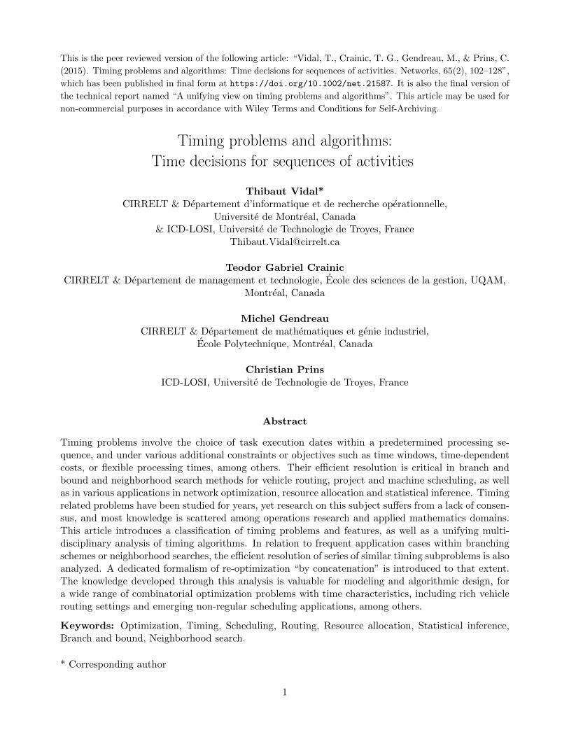
Surveying the literature, we distinguish two main categories of methods: those who maintain pri-mal feasibility, and those who maintain dual feasibility. These algorithms are issued from variousdomains. In the case of isotonic regression in particular, only precedence constraints among decisionvariables are considered (pi = 0 for all i), yet the associated methods can be extended to solve prob-lems with processing times with only minor modifications. We illustrate all algorithms on a simpleproblem, for which the cost functions and the processing times are given in Figure 2.

Primal methods. A first category of methods is based on respecting the primal feasibility conditionsand iteratively restoring the dual conditions. The first method of this kind, called Minimum Lower

9

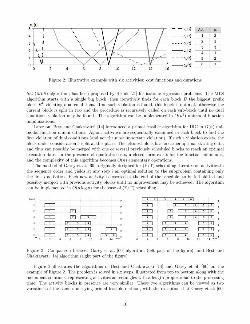
Figure 2: Illustrative example with six activities: cost functions and durations

Set (MLS ) algorithm, has been proposed by Brunk [21] for isotonic regression problems. The MLSalgorithm starts with a single big block, then iteratively finds for each block B the biggest prefixblock Bk violating dual conditions. If no such violation is found, this block is optimal, otherwise thecurrent block is split in two and the procedure is recursively called on each sub-block until no dualconditions violation may be found. The algorithm can be implemented in O(n2) unimodal functionminimizations.

Later on, Best and Chakravarti [14] introduced a primal feasible algorithm for IRC in O(n) uni-modal function minimizations. Again, activities are sequentially examined in each block to find thefirst violation of dual conditions (and not the most important violation). If such a violation exists, theblock under consideration is split at this place. The leftmost block has an earlier optimal starting date,and thus can possibly be merged with one or several previously scheduled blocks to reach an optimalexecution date. In the presence of quadratic costs, a closed form exists for the function minimums,and the complexity of this algorithm becomes O(n) elementary operations.

The method of Garey et al. [60], originally designed for (E/T) scheduling, iterates on activities inthe sequence order and yields at any step i an optimal solution to the subproblem containing onlythe first i activities. Each new activity is inserted at the end of the schedule, to be left-shifted andpossibly merged with previous activity blocks until no improvement may be achieved. The algorithmcan be implemented in O(n log n) for the case of (E/T) scheduling.

Figure 3: Comparison between Garey et al. [60] algorithm (left part of the figure), and Best andChakravarti [14] algorithm (right part of the figure)

Figure 3 illustrates the algorithms of Best and Chakravarti [14] and Garey et al. [60] on theexample of Figure 2. The problem is solved in six steps, illustrated from top to bottom along with theincumbent solutions, representing activities as rectangles with a length proportional to the processingtime. The activity blocks in presence are very similar. These two algorithms can be viewed as twovariations of the same underlying primal feasible method, with the exception that Garey et al. [60]

10

considers non-inserted activities as non-existing in the current solution, whereas Best and Chakravarti[14] maintains these non-scheduled activities in one final block which does not respect Condition 3.

The method of Garey et al. [60] was extended by Lee and Choi [101] and Pan and Shi [115] toaddress (E/T) scheduling problems with distinct penalty weights for earliness and tardiness, that isD,R(di = ri)|ø, in O(n log n) elementary operations. Szwarc and Mukhopadhyay [138] and Fengand Lau [53] also proposed to identify the tasks that are necessarily processed without idle time (inthe same block) before solving. Chretienne and Sourd [26] applied the algorithm to project schedul-ing with piecewise convex cost functions, and Hendel and Sourd [75] to timing problems with convexpiecewise linear or quadratic costs. These algorithms work in a linear number of unimodal functionminimizations, but differ in terms of the data structures used to represent the functions and thus onthe complexity of the function minimizations. When the cost functions are Piecewise Linear (PiL), themethod of Hendel and Sourd [75] attains a complexity of O(ϕc log n), where ϕc is the total number ofpieces in the activity cost functions of the sequence. Finally, Davis and Kanet [34] proposed anotherprimal method for (E/T) scheduling similar to Garey et al. [60], and generalized to PiL convex costsby Wan and Yen [151]. Activities are iteratively added to the solution in reverse sequence order. Eachactivity is scheduled at date 0, and then shifted onwards (while possibly merging blocks), until noimprovement can be achieved.

Dual feasible methods. Simultaneously with the MLS algorithm, another seminal method for IRCwas proposed by Ayer et al. [4] under the name of Pool Adjacent Violators (PAV ). Starting withan initial solution consisting of n separate blocks, one for each activity, successive pairs of blocks(Bi, Bi+1) not satisfying primal conditions are iteratively identified. Such blocks are merged, and thenext iteration is started. The order in which these block couples are identified does not affect the finalresult of the algorithm. An illustration of the method on the previous example is given in Figure 4.The algorithm iteratively merges the first pair of blocks that does not verify primal conditions. Wenotice that the optimal solution is reached after three merges (at Step 3).

Figure 4: The PAV algorithm illustrated on timing problems

Chakravarti [23] proved that PAV is a dual feasible method for the linear problem when the distanceconsidered is ‖ ‖1 (c(t) = Σ|ti − Ni|), while Grotzinger and Witzgall [65] and Best and Chakravarti[14] showed that PAV is a dual algorithm for IRC with quadratic costs (Euclidean distance).

The PAV algorithm was also generalized to convex functions by Best et al. [15] and Ahuja andOrlin [1], achieving a complexity of O(n) unimodal minimizations. It is noteworthy that, under atotally different formalism, an equivalent algorithm was discovered by Dumas et al. [46] for a generalvehicle routing setting with convex time-dependent service costs. For IRC with the ‖ ‖1 distance, thePAV algorithm can be implemented in O(n log2 n) elementary operations using balanced search trees[117], or O(n log n) complexity using scaling techniques [1]. Finally, O(n) algorithms are known forquadratic objectives [46, 65, 116].

11

5.4 Separable costs and multiple time windows

Without the previous convexity assumption, the timing problems Σci(ti)|ø become more complex,and many authors have focused on separable PiL costs. The feature MTW especially [27, 144] canalso be linearly reduced to a Σci(ti)|ø problem when a closed form representation of the multipletime windows, such as a list of feasible intervals, is available.

In the presence of non-negative and Lower Semi-Continuous (LSC) costs (ci(ti) ≤ limε→0 minci(ti+ε), c(ti − ε) at every discontinuity point), the timing problem Σci(ti)|ø can be efficiently solved bydynamic programming. A large range of backward and forward approaches has thus been proposed inthe routing and scheduling literature by Hendel and Sourd [74], Ibaraki et al. [86], Sourd [135], Yanoand Kim [152] and Ibaraki et al. [87].

Solving Σci(ti)|ø by forward dynamic programming involves the forward minimum cost functionFi(t), which evaluates the minimum cost to execute the sequence of activities (a1, . . . , ai) while startingthe last activity before or at time t (ti ≤ t). Fi(t) functions can be computed by means of Equation(19), starting from the case i = 1 with a single activity where F1(t) = minx≤t c1(x). The optimalsolution value of the timing problem is z∗ = Fn(+∞), and the optimal activity execution dates canbe retrieved from the Fi(t) functions.

Fi(t) = min0≤x≤t

ci(x) + Fi−1(x− pi−1) 1 < i ≤ n (19)

The symmetric way to solve this problem by backward programming involves the backward min-imum cost function Bi(t), which evaluates the minimum cost to execute the sequence of activities(ai, . . . , an), while executing the first activity ai after or at time t (ti ≥ t). Bi(t) functions are com-puted by backward recursion, starting with Bn(t) = minx≥t cn(x) and using Equation (20). Theoptimal solution value of the timing problem is z∗ = B1(−∞).

Bi(t) = minx≥tci(x) +Bi+1(x+ pi) 1 ≤ i < n (20)

These methods can be implemented in O(nϕc), where ϕc stands for the total number of pieces inthe activity cost functions ci. When the costs are also convex, the use of efficient tree data structuresleads to a complexity of O(ϕc logϕc) [87], matching the best available approaches in O(n log n) for theparticular cases related to IRC, (E/T) scheduling, and soft time windows.

5.5 State-of-the-art: single-dimensional features

As illustrated by this section, single-dimensional features are related to many prominent problemssuch as LISP and IRC, which have been the subject of extensive research. Various algorithms wereexamined and state-of-the-art methods for each particular feature and problem were identified. In theparticular case of Σccvxi (ti)|ø, 26 methods from various fields such as routing, scheduling and isotonicregression were classified into three main families: primal, dual, and dynamic programming methods.Efficient linearithmic methods are known for a very general problem of this category, Σccvxi (ti)|ø,in the presence of either convex or LSC and piecewise linear cost functions. Still, as illustrated inSection 7, the resolution of series of similar timing instances during a local search can be performedmore efficiently by means of re-optimization procedures.

6 Two-dimensional features

We now focus on the problems with two-dimensional features. These features are also often consideredin the presence of time-window TW constraints. The presentation is structured in relation to thelevel of problem complexity and generality. Starting with the duration feature DUR, which involves

12

exclusively the first and last activities together, we then examine two-dimensional features involvingsuccessive activities: no-wait NWT , idle time IDL, and flexible ci(∆ti) or time-dependent P (t)processing times. Finally, features involving any pair of activities, such as time-lags TL, and costfunctions separable by pairs of variables Σcij(ti, tj) are analyzed.

6.1 Total duration and total idle time

Accounting for total duration or idle-time is meaningful when one has the possibility to delay thebeginning of operations. Otherwise, considering the maximum execution date feature C is sufficient.Whereas delaying the start of production is generally not an option in scheduling problems, it becomesparticularly relevant in routing, as real-life objectives and driver’s wages are frequently based onduration. We mention Savelsbergh [132] for duration minimization under time-window and durationconstraints in VRPs, Cordeau et al. [31] that generalizes the previous approach for soft time-windowsand duration constraints, Desaulniers and Villeneuve [37] for shortest path settings with linear idle-time costs and time windows, and Desaulniers et al. [38] and Irnich [91] for a general framework whichaddresses duration and idle time features, among others, in various time-constrained routing and crewscheduling problems. It should be noted that computing the total duration or the total idle time isequivalent in the presence of fixed processing times. Therefore, without loss of generality we will focuson duration in this section.

To manage duration features in DUR|TW and ø|DUR, TW, Savelsbergh [132] proposed tofirst rely on a minimum idle time policy, and then shift activity execution dates forward to reduce thetotal duration. The related amount of shift was introduced many years ago in the project schedulingliterature [105] as the latest processing date for an activity that does not cause a delay in the calendar.It is also known in the VRP literature under the name of forward time slack [131, 132]. The followingquantities are computed for each activity ai: the earliest feasible execution date Ti, the cumulative idletime Wi on the subsequence (a1, . . . , ai) according to these execution dates, and the partial forwardtime slack Fi on the subsequence (a1, . . . , ai). These values are computed recursively by means ofEquations (21-23), starting with the case of a single activity where T1 = r1, W1 = 0 and F1 = d1− r1.

Ti = max(Ti−1 + pi−1, ri) 1 < i ≤ n (21)

Wi = Wi−1 + Ti − Ti−1 − pi−1 1 < i ≤ n (22)

Fi = min(Fi−1, di − Ti +Wi) 1 < i ≤ n (23)

The problem admits a feasible solution if and only if Ti ≤ di for all i. The execution date of thefirst activity in an optimal solution is given by t∗1 = r1 + minFn,Wn. The other dates are computedusing the minimum idle time policy. Both feasibility checking and duration minimization problemsare thus solved in O(n). Desaulniers and Villeneuve [37], Kindervater and Savelsbergh [97] and Irnich[91] proposed different calculations of this optimal schedule. As pointed out in Parragh et al. [118],all these approaches are equivalent.

Tricoire et al. [144] recently considered a more complex timing problem aiming to minimize du-ration under MTW constraints DUR|MTW. Each activity ai is associated with a set of ki timewindows, MTWi = [ri1, di1], . . . , [riki , diki ]. The authors proposed a procedure that first removessome unnecessary time-window segments, not suitable for any feasible solution, while detecting infea-sible timing problems. In a second step, the procedure examines a subset of dominant schedules, suchthat “no better solution exists with the same last activity execution date”. For a given execution datetn of the last activity, a dominant schedule with minimum duration can be found using the backwardrecursion of Equation (24).

ti−1 = maxt | t ≤ ti − pi−1 ∧ t ∈MTWi (24)

13

Starting from the dominant schedule t with earliest completion time, the method iteratively iden-tifies the last activity ai followed by idle time: ti + pi < ti+1. If activity ai does not admit a later timewindow, the algorithm terminates. Otherwise, the execution date of activity ai is set to the beginningof the next time window, and the execution dates of activities situated afterwards in the sequence arere-computed with a minimum idle time policy. This leads to a dominant schedule which becomes tin the next iteration. Tricoire et al. [144] proved that at least one dominant schedule explored in thecourse of the algorithm is optimal. If each customer is associated to at least one time window, theoverall method can be implemented in O(nϕmtw), ϕmtw representing the number of time windows inthe problem.

Figure 5: Duration minimization under multiple time-window constraints

This algorithm is illustrated in Figure 5 on a small example with four activities. Activities arerepresented from bottom to top with their time windows. The earliest completion date is computedwith a minimum idle time policy, illustrated in gray lines. The initial dominant schedule t0 , in black, isthen determined by backward recursion using Equation (24). This schedule presents waiting time afteractivity a3, and thus the execution date of this activity is delayed to the next time window, leading toa dominant schedule t1. Now the latest activity followed by waiting time is a2. Its execution date isdelayed, and leads to the dominant schedule t2. The latest activity followed by waiting time is a1. Asthere is no later time window for this activity, the algorithm terminates. Among the three dominantschedules explored by the method, the best solution with minimum duration has been reached by t2,and is optimal.

6.2 No wait and idle time

No-wait NWT and idle-time IDL features appear in various settings involving, among others, deterio-ration of products, maximum waiting times in passenger transportation, fermentation processes in thefood industry, and cooling in metal-casting processes. IDL reduces to NWT when the maximum idletime is set to ιi = 0. No-wait constraints ti = ti+1 can also be addressed by problem reformulation,merging unnecessary variables. When no waiting time is allowed on the entire activity sequence, thetiming problem becomes a minimization problem of a sum of single-variable functions. Two maincategories of problems have been considered in the literature for NWT and IDL: the feasibility prob-lem under idle-time and time-window constraints, and the optimization problem when some of thesefeatures appear in the objective function, treated in Section 6.3 in a more general context.

Feasibility checking under maximum idle time and time-window constraints has been frequentlystudied in the routing literature. Hunsaker and Savelsbergh [82] designed an algorithm to checkthe feasibility of itineraries in dial-a-ride settings. This algorithm contains a O(n) checking methodfor the special case of ø|IDL, TW. The solution to ø|IDL, TW is found in two scans of theactivity sequence. The first pass considers the relaxed subproblem ø|TW, determining for each

14

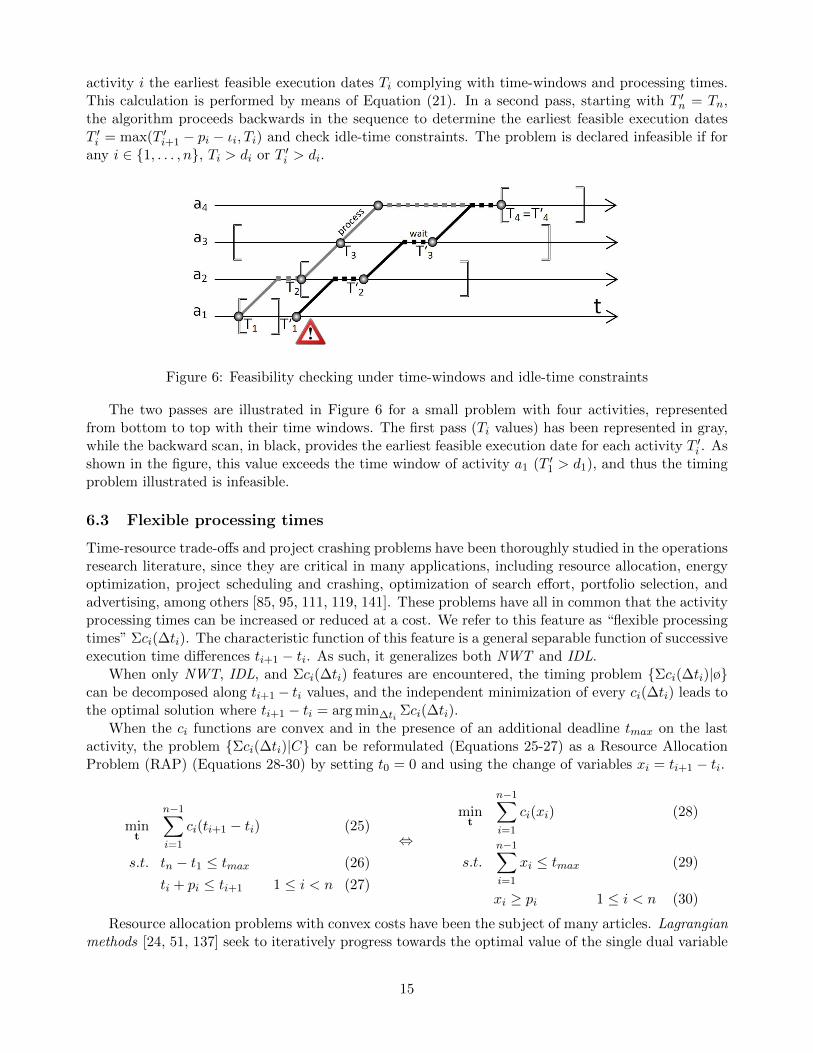
activity i the earliest feasible execution dates Ti complying with time-windows and processing times.This calculation is performed by means of Equation (21). In a second pass, starting with T ′n = Tn,the algorithm proceeds backwards in the sequence to determine the earliest feasible execution datesT ′i = max(T ′i+1 − pi − ιi, Ti) and check idle-time constraints. The problem is declared infeasible if forany i ∈ 1, . . . , n, Ti > di or T ′i > di.

Figure 6: Feasibility checking under time-windows and idle-time constraints

The two passes are illustrated in Figure 6 for a small problem with four activities, representedfrom bottom to top with their time windows. The first pass (Ti values) has been represented in gray,while the backward scan, in black, provides the earliest feasible execution date for each activity T ′i . Asshown in the figure, this value exceeds the time window of activity a1 (T ′1 > d1), and thus the timingproblem illustrated is infeasible.

6.3 Flexible processing times

Time-resource trade-offs and project crashing problems have been thoroughly studied in the operationsresearch literature, since they are critical in many applications, including resource allocation, energyoptimization, project scheduling and crashing, optimization of search effort, portfolio selection, andadvertising, among others [85, 95, 111, 119, 141]. These problems have all in common that the activityprocessing times can be increased or reduced at a cost. We refer to this feature as “flexible processingtimes” Σci(∆ti). The characteristic function of this feature is a general separable function of successiveexecution time differences ti+1 − ti. As such, it generalizes both NWT and IDL.

When only NWT, IDL, and Σci(∆ti) features are encountered, the timing problem Σci(∆ti)|øcan be decomposed along ti+1 − ti values, and the independent minimization of every ci(∆ti) leads tothe optimal solution where ti+1 − ti = arg min∆ti Σci(∆ti).

When the ci functions are convex and in the presence of an additional deadline tmax on the lastactivity, the problem Σci(∆ti)|C can be reformulated (Equations 25-27) as a Resource AllocationProblem (RAP) (Equations 28-30) by setting t0 = 0 and using the change of variables xi = ti+1 − ti.

mint

n−1∑i=1

ci(ti+1 − ti) (25)

s.t. tn − t1 ≤ tmax (26)

ti + pi ≤ ti+1 1 ≤ i < n (27)

⇔

mint

n−1∑i=1

ci(xi) (28)

s.t.

n−1∑i=1

xi ≤ tmax (29)

xi ≥ pi 1 ≤ i < n (30)

Resource allocation problems with convex costs have been the subject of many articles. Lagrangianmethods [24, 51, 137] seek to iteratively progress towards the optimal value of the single dual variable

15

associated to Equation (29) while respecting primal feasibility. Pegging algorithms [98, 102, 130] relaxthe constraints of Equations (29-30), iteratively solving the relaxed problems and fixing the valuesof variables that do not satisfy primal constraints. Dynamic programming can also be efficientlyapplied [93]. Σccvxi (∆ti)|C with integer variables can be addressed in O(n log tmax

n ) [58, 77], and anε-approximate solution can be found in O(n log tmax

εn ) for the continuous version [77].In the presence of polymatroidal constraints, convex resource allocation problems can be solved

to optimality by a greedy algorithm iteratively incrementing the least-cost variable. Hochbaum [77]proposes a greedy algorithm with scaling for Σccvxi (∆ti)|C,D, which produces an ε-approximatesolution in O(n log n log tmax

εn ). This problem appears in various application contexts, such as lot sizing[142], assortment with downward substitution [120], and telecommunications [113], among others.Let m be the number of deadline constraints. The problem Σccvxi (∆ti)|C,D with continuous orinteger variables can be solved in O(n logm log tmax

ε ) and O(n logm log tmaxn ), respectively, with the

decomposition approach of Vidal et al. [149]. Finally, the quadratic Σccvxi (∆ti)|C,D with continuousvariables can be addressed in O(n log n) [78] or O(n logm) [149].

Adding time-window constraints to the model of Equations (25-27) leads to other timing set-tings and resource allocation problems with non-polymatroidal constraints. In the special case ofNorstad et al. [111], a timing problem Σccvxi (∆ti)|TW is addressed with the objective z(t) =∑n

i=1 di,i+1c((ti+1 − ti)/di,i+1) and non-increasing and convex c(∆t) functions (independent of theactivity). In the presence of such functions, relaxing time-window constraints leads to an optimal so-lution with constant ratio (ti+1− ti)/di,i+1 for all i, and thus constant speed on all legs. The recursivesmoothing algorithm (RSA) exploits this property by maintaining this ratio constant on subsequencesand progressively re-introducing violated time-window constraints. The overall method works in O(n2)elementary operations once the minimum of each function c(∆t) is given. This method is a dual feasi-ble algorithm based on the relaxation and re-introduction of window constraints. It is closely relatedto the “string” methodology described in [33] and also discussed in [149].

Sourd [135] and Hashimoto et al. [70] have independently studied Σci(∆ti),Σci(ti)|ø (Equation31) with piecewise linear functions in the context of (E/T) scheduling and vehicle routing, and reportits NP-hardness.

min(t1,...,tn)∈<n+

n∑i=1

ci(ti) +

n−1∑i=1

ci(ti+1 − ti) (31)

When the functions ci and ci are PiL with integer breakpoints, a dynamic programming algorithmis proposed to solve the problem in O(T 2), where T represents an upper bound on the schedule dura-tions. This dynamic programming algorithm can be viewed as an extension of the resource allocationalgorithm of Karush [93]. The method can be implemented with a forward dynamic programmingfunction Fi(t) (Equations 32-33), which evaluates the minimum cost to process the subsequence ofactivities (a1, . . . , ai), starting the last activity exactly at time t (ti = t). The resulting optimal costis given by z∗ = mint Fn(t).

F1(t) = c1(t) (32)

Fi(t) = ci(t) + min0≤x≤t

Fi−1(x) + ci−1(t− x) 1 < i ≤ n (33)

A polynomial dynamic programming algorithm working in O(nϕc + nϕc × ϕc) exists for the casewhere the functions ci(∆t) are PiL and convex [70, 135]. ϕc and ϕc represent the total number of piecesin the cost functions ci and ci, and ϕc stands for the number of convex pieces in the cost functions ci.Efficient re-optimization procedures have also been proposed (Section 7).

Finally, DUR involved in the objective can be seen as a special case of Σci(∆ti) where cduri (∆ti) =∆ti. MTW is also reducible to Σci(ti), and thus the previous algorithm provides an alternative way tosolve DUR|MTW or ø|DUR,MTW in O(n+ nϕmtw), where ϕmtw represents the total numberof time windows.

16

6.4 Time-dependent processing times

In several application settings, activity processing times may vary as a function of the executiondates. In machine and project scheduling for example, learning, deterioration effects and other time-dependencies can have a large impact [3, 25]. Network congestion is a major concern for vehicle routingand data transmission [99, 145] and, thus, the time-dependent processing-time feature P (t) appearsin various network optimization problems: shortest path [28, 44, 67], traveling salesman [104], andvehicle routing [11, 43, 71, 88, 103], among others.

The literature on the subject can generally be separated between discrete and continuous settings.Discrete optimization models generally involve time-space networks which are less likely to presentthe timing issues studied in this article, whereas several continuous models have led to explicit timingproblems with P (t) features, as in Donati et al. [43], Fleischmann et al. [56], Ichoua et al. [88], andHashimoto et al. [71]. These models involve constraints of the type ti + pi(ti) ≤ ti+1 within a timingformulation with other additional features.

The FIFO assumption on functions pi is often valid. FIFO implies that any delay in an activityexecution date results in a delay in its completion date. The assumption is meaningful in severalsettings, e.g. vehicle routing, as two vehicles that behave similarly on the same route are supposed toremain in the same arrival order, whatever congestion happens [88].

FIFO assumption: ∀i x ≥ y =⇒ x+ pi(x) ≥ y + pi(y) (34)

Time-dependent processing-time features are generally assumed to result in more complex tim-ing problems. However, one should clearly identify the source of the difficulty, which is frequentlyimputable to the computation and access to pij(t) throughout the search, and not necessarily to thetiming problem resolution. Assuming that pij(t) can be evaluated in constant time and under FIFO,D|R,P (t) is still solvable in O(n) by means of a minimum idle time policy [56] and the time-slackapproach of Savelsbergh [132] can still be applied [43] to ø|TW,P (t). Still, dedicated methodologiesare necessary for other settings such as DUR|TW,P (t).

The time-dependent timing problem Σci(ti)|P (t), Equations (35-36), is addressed in Hashimotoet al. [71]. All functions considered are PiL, non-negative and lower semicontinuous.

min(t1,...,tn)∈<n+

n∑i=1

ci(ti) (35)

s.t. ti + pi(ti) ≤ ti+1 1 ≤ i < n (36)

The authors propose a dynamic programming approach, which extends the method of Section 5.4. Itinvolves the functions Fi(t), which represent the minimum cost to process the subsequence of activities(a1, . . . , ai) while starting the last activity before t (ti ≤ t). Under the assumption of Equation (37),which is weaker than FIFO, the method can be implemented in O(nϕc + nϕp), where ϕc and ϕp arethe total number of pieces in cost and processing-time functions.

(HYI) assumption: ∀i x+ pi(x) = y + pi(y) =⇒ x+ pi(x) = z + pi(z) ∀z ∈ [x, y] (37)

This method for Σci(ti)|P (t) thus presents the same quadratic complexity as in the case withouttime dependency (Section 5.4). When the previous assumption does not hold, the dynamic program-ming method of Hashimoto et al. [71] is not polynomial, and the question remains open whetherΣci(ti)|P (t) is polynomially solvable.

6.5 Time lags

The two-dimensional features surveyed in the previous sections involved linking constraints and ob-jectives between the first and last tasks, in the case of DUR, or between pairs of successive variables

17

in the case of NWT and IDL. We now review the time-lag TL feature, which brings into play atime difference tj − ti between any two activity execution dates ti and tj . This feature is thus ageneralization of NWT , IDL and DUR.

To the best of our knowledge, early research on time lags has been conducted by Mitten [107] forflowshop scheduling problems. This feature has been used since to model many problem characteristicsin various domains, such as the deterioration of food or chemical products, glue drying, customerrequirements in some dial-a-ride problems, elevator dispatching, quarantine durations, and so on.Time-lag scheduling problems on a single machine have also been shown by Brucker et al. [20] togeneralize all shop, multi-purpose machines, and multi-processor scheduling problems. Hence, timingproblems with TL are likely to be difficult.

The most basic problem with TL feature relates to feasibility checking under time-lag constraintsof the form ti + δij ≤ tj . When δij ≥ 0, the constraint is called positive time lag, and correspondsto a minimum delay between activities ai and aj , whereas δij ≤ 0 corresponds to a negative timelag, and involves a maximum delay of −δij between the activities aj and ai. Equality constraintsti + δij = tj involve both positive and negative time lags. The resulting timing problem ø|TL canbe seen as a special case of project scheduling on a chain of activities, and the METRA potentialmethod (MPM) of Roy [128, 129] can be applied. In MPM, the time-lag constraints are representedon a graph G = (V,A), where each activity ai is associated with a node vi ∈ V , and each arc (vi, vj),associated with a weight wij , represents a temporal constraint of the form tj− ti ≥ wij . The feasibilityof ø|TL is equivalent to the non-existence of a positive length cycle in this graph [9, 35]. Thealgorithm of Floyd-Warshall can be employed to solve this problem in O(n3), but the longest-pathprocedure of Hurink and Keuchel [83], also in O(n3), is shown to provide faster results in practice.Potts and Whitehead [122] also considered a coupled-operation scheduling problem with only n/2 time-lag constraints, and timing feasibility is checked in O(n2). The authors underlined the computationalburden of such timing algorithms, which strongly degrades the performance of neighborhood searchesor branch and bound procedures.

Hunsaker and Savelsbergh [82] studied a case of ø|TL, TW timing in the context of dial-a-rideproblems. Activities represent customer requests on pick-up and deliveries services, which occur bypairs, such that any pick-up always precedes its corresponding delivery in the sequence. Each such pairof activities is linked by a single positive time-lag constraint. The total number of time-lag constraintsis thus n/2. The problem also involves time windows and maximum idle times for each activity. Theauthors claim that the resulting feasibility problem can be solved in three passes on the sequence ofactivities with linear complexity. Yet, the algorithm presents a small flaw, which is straightforward tocorrect [143], but leads to a O(n log n) complexity [73]. A O(n) complexity is finally achieved in Firatand Woeginger [54] by means of a reduction to a shortest path problem on a weighted interval graph.

The same setting is also addressed in Gschwind and Irnich [66]. The authors describe a labelingprocedure based on |Mi| resources for each pickup and each delivery activity ai. Mi stands for thecurrent number of open pickups at ai. This labeling procedure provides another way to check the fea-sibility of a fixed activity sequence ø|TL, TW in O(n2). Furthermore, the feasibility of an extendedsequence with one additional activity an+1 can be evaluated in O(Mn+1) given the information onthe original sequence. Such forward extension function is critical when solving shortest path problemswith underlying timing features.

Cordeau and Laporte [29] and Berbeglia et al. [12] consider a dial-a-ride setting with an additionalduration constraint on the entire trip duration. The authors solve heuristically a Lagrangian relaxationof the problem with a hierarchical objective. Total trip duration infeasibility is minimized, thentime-window infeasibility and, finally, time-lag infeasibility, that is the timing problem DUR >D > TL|R. The algorithm first minimizes duration and time-window infeasibility as in Section6.1, then iteratively delays some pick-up services to reduce time-lag infeasibility without increasingany other violation. A computational complexity of O(n2) is achieved. It was observed in a private

18

communication, however, that the previous approach only guarantees optimality under an additionalassumption that we call LIFO, which requires that for any 1 ≤ i < j < k < l ≤ n, no activitiesai, aj , ak, al present “entangled” time-lag constraints of the form tk − ti ≤ δik and tl − tj ≤ δjl. TheLIFO assumption is frequently enforced in the vehicle routing literature, especially when transportingpassengers, or in the presence of complex loading constraints. In this case, the last object or customerreceived in the vehicle is the first one to leave. Without this assumption, the difficulty of manyproblems with time lags strongly increases, and no specialized efficient algorithm is actually knownfor DUR > D > TL|R and similar problems.

6.6 Separable costs by pairs of variables

Separable costs by pairs of variables Σcij(ti, tj) generalize all problems combining single or two-dimensional features. The timing problem with this feature alone is NP-hard in the presence ofpiecewise linear functions since it generalizes Σci(ti),Σci(∆ti)|ø. When the objective function isconvex, the problem Σccvxij (tj − ti),Σccvxi (ti)|ø is equivalent to the convex cost dual network flowproblem, and a weakly polynomial algorithm is provided in Ahuja et al. [2].

6.7 State-of-the-art : “stand-alone” timing methods

In contrast to single-dimensional features, which appeared as fairly well addressed in Section 5 bymeans of a few algorithms and concepts, two-dimensional features lead to more diverse problem struc-tures and algorithms. Several simple cases with duration minimization or time-dependent processingtimes can be solved in linear time, but other problems with time-lag features actually require O(n3)algorithms to be solved exactly. Although polynomial, the latter methods can be impracticable in thecontext of local searches or branch-and-bound approaches.

Many practical timing settings result in models with linear constraints and linear or separableconvex objectives. For these problems, the linear and convex programming theory ensures weaklypolynomial resolvability, and provides general solution methods [79, 92, 96]. Some more generalproblems, however, such as Σci(ti),Σci(∆ti)|ø with PiL functions, are NP-hard, while for otherproblems, such as Σci(ti)|P (t) with general piecewise linear functions P (t), the existence or non-existence of polynomial algorithm is still open. Timing settings thus lead to a rich variety of problemstructures and complexities.

In all these cases, whether polynomial algorithms are available or not, research is still open toprovide more efficient algorithms exploiting the particular structure of the features and problems athand. The present paper contributed by building a formalism, a classification of features, timingproblems and methods. We gathered the most efficient stand-alone timing approaches from variousfields of research to tackle both specialized timing settings, and more general features. The focuscan now be turned on filling the gaps that have been highlighted in this review, and which continueto appear, following the rich variety of application cases with time constraints emerging nowadays.Finally, important avenues of research target the efficient solving of series of timing problems, in theparticular context of neighborhood searches and branch-and-bound. Such approaches are presentedin the next section.

7 Timing re-optimization

In previous sections, we examined how to address timing problems as a stand-alone issue. Yet, mostneighborhood-search-based heuristics, metaheuristics, and some exact methods require to solve iter-atively a large number of closely related timing instances. In this case, solving each timing problem

19

“from scratch”, without exploiting any knowledge on previous resolutions, can result in losses of in-formation and redundant computations.

Most local searches for routing and scheduling problems (see [81] for a presentation of local search)rely on a neighborhood based on a limited number of sequence changes. One or several timing sub-problems are solved for each neighbor to estimate its feasibility and cost. Figure 7 illustrates twoclassical neighborhoods to change sequences of activities, 2-opt* which exchanges the tails of twosequences of activities [123], and Or-opt to relocate a subsequence of consecutive activities [112].It is noticeable that large subsequences of activities, SeqA, SeqB, SeqC and SeqD on the figure, areshared by successive timing subproblems. Branch-and-bound procedures for problems with sequenc-ing decisions can similarly involve timing subproblems at nodes of the search tree when evaluatingsequences of activities, during lower bound computation and branch pruning [80, 136]. The searchfor improving columns, in column generation approaches, also frequently involves elementary shortestpaths with timing decisions and resource constraints [7, 41, 124].

Seq. A

Seq. C

Seq. B

Seq. D

Time

Seq. A

Seq. C

Seq. D

1

2

3

4

5

6

7

8

9

10

Seq. B

1 2 3 4 6 7 5 8

Figure 7: A 2-opt* local search move (left) and an Or-opt move (right)

In all these cases, numerous closely related timing problems must be solved, where long subse-quences of consecutive activities remain unchanged, and only a minor proportion of problem param-eters (reduced cost values for column generation) is impacted. Several authors thus propose to keepmeaningful data on the global search process to save computations and solve more efficiently theseseries of similar timing problems. Neighborhood searches largely benefit from such techniques, asmove evaluations (and thus the resolution of timing problems) take the largest part of the computa-tional effort. These re-optimization methodologies therefore can lead to significant reductions in thecomputational burden of algorithms.

We now formally define serial timing problems in Section 7.1, and present a general frameworkfor re-optimization methods based on sequence concatenations in Sections 7.2-7.3. Links with relatedre-optimization methodologies are analyzed in Section 7.4, before reviewing or introducing efficientconcatenation-based re-optimization methods for each major timing feature and related problems inSection 7.5.

7.1 Problem statement: Serial timing

This section formally defines serial timing problems. Sequence-dependent processing times are alsoconsidered, in relation to a large range of vehicle routing applications which rely extensively on re-optimization methods.

Definition 5 (Serial timing). Let T be an incumbent timing problem with n activities (a1, . . . , an),sequence-dependent processing-times pij, and additional features with characteristic functions, fxy (t),separated into two sets Fobj and Fcons following their role as objective or constraint (Section 2). Npermutation functions σk : 1, . . . , n → 1, . . . , n for k ∈ 1, . . . , N, are also given. The serial

20

timing problem involves to solve the timing subproblems T k of Equations (38-40), for k ∈ 1, . . . , N.

(T k) : mint=(t1,...,tn)∈<n+

∑Fx∈Fobj

αx∑

1≤y≤mx

fxy (t) (38)

s.t. tσk(i) + pσk(i),σk(i+1) ≤ tσk(i+1) 1 ≤ i < n (39)

fxy (t) ≤ 0 F x ∈ Fcons , 1 ≤ y ≤ mx (40)

To efficiently solve the previous problem, several types of re-optimization approaches have beendeveloped in the literature to take advantage of the information developed during the successivesubproblem solving. One such approach involves re-arranging previously developed schedules in re-lation to the new settings. For network-flow or shortest-path formulations especially, re-optimizationmethods related to a change of arcs or costs in the network have been studied over a long period[57, 63, 106, 114]. Most timing problems can also be formulated as linear program. Sensitivity analy-sis and warm start following a problem modification may be done by means of a primal-dual simplexalgorithm. Finally, a last methodology, on which we focus in the following, is based on the observationthat a permutation of activities can be assimilated to a concatenation of some subsequences of con-secutive activities. Hence, managing information on subsequences (e.g., dynamic programming labels)can lead to significant resolution speed ups [32, 97].

7.2 Breakpoints and concatenations

We first introduce some vocabulary, and then emphasize the links between operations on sequences ofactivities, such as changes of precedence and activity relocations, and the properties of the resultingpermutation functions. These observations lead to efficient re-optimization approaches.

Definition 6 (Permutation breakpoints). Let σ : 1, . . . , n → 1, . . . , n be a permutation. Anyinteger b such that σ(b) + 1 6= σ(b + 1) and 1 ≤ i < n is called a breakpoint of σ, and corresponds tonon-consecutive values in the permutation representation.

Let b(σ) denote the number of breakpoints of σ, and bσ1 , . . . , bσb(σ) denote these breakpoints in

increasing order. For instance, the permutation σ0 : 1, 2, 3, 4, 5, 6 → 4,5,3, 1,2, 6 has threebreakpoints (indicated in boldface): bσ01 = 2, bσ02 = 3, and bσ03 = 5. We now show the links betweenclassical operations on activity sequences and the resulting permutation function properties in termsof breakpoints. Two main operations can be considered. The first operation is a change of precedencebetween two activities. For example, two precedences are changed on the left of Figure 7: activity3 now precedes activity 9 instead of 4, and activity 8 precedes activity 4 instead of 9. The secondoperation is the relocation of a sequence of activities. For example, on the right of the figure, thesequence of activities 3, 4 is relocated between activities 6 and 7.

Lemma 1 (Precedence changes). Let A′ be an activity sequence obtained from A by changing l prece-dence relations and σA→A′ the associated permutation function, then b(σA→A′) = l.

Lemma 2 (Activity relocations). Let A′ be an activity sequence obtained from A by relocating lactivities and σA→A′ the associated permutation function, then b(σA→A′) ≤ 3l.

Any change of the precedence relation results in exactly one breakpoint while any relocation ofactivity can be assimilated to at most three changes of precedence relations, and thus yields threebreakpoints. Situations where k precedence relations are changed from one timing problem T toanother problem T ′ occur frequently in the context of neighborhood searches for combinatorial opti-mization problems with sequence optimization, e.g., vehicle routing or machine scheduling. A timingsubproblem may need to be solved to evaluate the cost and feasibility of each new sequence in the

21

presence of complicating time constraints. The interest of breakpoints is highlighted in the followingproposition. Although straightforward, it provides the basis of re-optimization methods working byconcatenation.

Proposition 1. Let σ : 1, . . . , n → 1, . . . , n be a permutation with breakpoints bσ1 , . . . , bσb(σ). Let

A be a sequence of n activities. Then, A′ = σ(A) corresponds to the concatenation of exactly b(σ) + 1subsequences of consecutive activities in A, as presented in Equation 41. A dummy breakpoint bσ0 = 1stands for the beginning of the sequence.

A′ =⊕

l=0,...,b(σ)−1

(aσ(bσl +1), . . . , aσ(bσl+1)) (41)

Any bounded number of operations transforming an activity sequence A into A′ (relocation ofactivities, or changes of precedence relations) thus involves a permutation function with a boundednumber of breakpoints, such that A′ can be seen as a concatenation of a bounded number of subse-quences of A. As shown in the following, the data, which is pre-processed from a bounded number ofsubsequences, may be extended to their concatenation, thus enabling to solve the timing subproblemsmore efficiently by exploiting existing knowledge.

7.3 Re-optimization “by concatenation”

Re-optimization by concatenation can be formalized by means of a set of four basic re-optimizationoperators. Three of these operators, initialization, forward extension and backward extensionare used to build re-optimization data on subsequences of activities from the incumbent timing prob-lem, while the last operator, evaluate concatenation, is specifically tailored to solve a new problem,more efficiently, using the existing re-optimization data on its subsequences of activities.

Initialization – Initialize the data D(A) of a sequence containing a single activity.Forward extension – Given an activity ak and a sequence A = (ai, . . . , aj) with its data, deter-

mine the data D(A′) for the sequence A′ = (ak, ai, . . . , aj).Backward extension – Given an activity ak and a sequence A = (ai, . . . , aj) with its data,

determine the data D(A′) for the sequence A′ = (ai, . . . , aj , ak).Evaluate concatenation – Given L sequences of activities D(Al), l = 1 . . . l and their data, eval-

uate the feasibility and the optimal solution cost of the timing problem involving the concatenationof these sequences.

The re-optimization approach illustrated in Algorithm 1 is based on these operators. Data is firstbuilt on subsequences of the incumbent timing problem T , by means of the forward and backwardextension operators. Since there are O(n2) such subsequences of consecutive activities, preprocessingcan be achieved appending iteratively O(n2) times one activity at the sequences’ end (or beginning).This preprocessing can be either performed before or during the search. The resulting data is thenexploited to solve the problems T k for k ∈ 1, . . . , N by means of the concatenation operator.

Consider a neighborhood search for routing problems with time constraints on routes. In thiscontext, a local search improvement procedure based on sequence changes leads to a number of timingsubproblems proportional to the number of neighborhood solutions to explore. The number of derivedtiming subproblems is usually N = Ω(n2), and the derived activity sequences do not involve theconcatenation of more than k = 2, 3 or 4 subsequences of the original problem.

The overall complexity of a neighborhood exploration, when solving each timing subproblem in-dependently, is Nc(T ), c(T ) being the computational complexity of one stand-alone timing solutionprocedure. A straightforward re-optimization approach consists in exhaustively computing the data

22

Algorithm 1 Re-optimization

1: Build re-optimization data on subsequences of the incumbent timing problem T , using initialize,and forward extension or backward extension.

2: For each timing subproblem T k, k ∈ 1, . . . , N;3: Determine the breakpoints involved in the permutation function σk;4: Evaluate the optimal cost of T k, as the concatenation of b(σ)+1 activity subsequences fromT (Equation 41).

for each of the n(n − 1) subsequences of consecutive activities from T , and then use it to evalu-ate all moves. Data computation is straightforward to perform in O(n2c(I) + n2c(F/B)). c(I) andc(F/B) stand for the computational complexity of initialization, and forward or backward exten-sion, respectively. The overall complexity of the new neighborhood exploration procedure is thusO(n2c(I) + n2c(F/B) + Nc(EC)), c(EC) being the complexity for evaluating the concatenation ofless than 4 subsequences. Assuming that N = Ω(n2), the computational complexity of neighborhoodevaluation becomes O(N [c(I) + c(F/B) + c(EC)]) for re-optimization methods instead of Nc(T ) forindependent solving. Re-optimization operators being less computationally complex than stand-alonemethods, the resulting approach is likely to lead to reduced computational effort. The efficiency ofAlgorithm 1 thus directly relies on the potential to develop concatenation operations that are lesscomputationally complex than stand-alone methods.

Concatenation operators involving more than two sequences are not actually available or notcomputationally suitable for efficient re-optimization for some settings such as ø|MTW and mostproblems with two-dimensional features. In this case, forward and backward propagation may beused along with concatenations of two subsequences only to perform the timing subproblem eval-uations. Such an example is given by the lexicographic search of Savelsbergh [131], which can beused to evaluate timing subproblems associated to some well-known neighborhoods for vehicle routingproblems exclusively by means of concatenation of two subsequence. Finally, if the concatenation ofmany subsequences can be operated efficiently, but data creation constitutes the bottleneck in termsof computational effort, the subset of subsequences involved can be restricted to O(n4/3) or O(n8/7),using the hierarchical approach of Irnich [90].

The relevant data to compute can also be tailored relatively to the neighborhoods at play. Forexample, the 2-opt* move presented in Figure 7 involves only the concatenation of subsequencescontaining the first or last activity, which we call prefix or suffix subsequences. The number of suchsubsequences requiring data computation is thus reduced to O(n).

7.4 General literature on the topic

A large range of vehicle routing and scheduling problems are addressed using local search on sequences.Serial timing issues thus frequently arise in these fields.

Following the seminal work of Savelsbergh [131, 132], Kindervater and Savelsbergh [97] proposed aframework to manage several constraints on vehicle routes, such as precedence constraints, time win-dows, collection and deliveries under capacity constraints. Several of these constraints are explicitly,or can be assimilated to, timing features. To perform efficient feasibility checking, the authors de-velop global variables on partial routes, which are used in concatenation operations to evaluate movesconsisting of a constant number of edge exchanges. Move evaluations are performed in lexicographicorder to allow calculation of the global variables through the search.

Cordone [32] and Duhamel [45] report similar concepts of global data management on subsequencesand concatenation operators. Although these methodologies are essentially dedicated to the VRPTW,they explore different possibilities related to the concept of macro-nodes. Indeed, when the information

23

developed on subsequences has the same structure as the problem data on activities, subsequences ofactivities can be replaced by equivalent single activities during timing resolution. In this case, thesize of the problem may be temporarily reduced by collapsing nodes into macro-nodes, leading toalgorithms based on aggregation of activities and multi-level approaches [10, 48, 150].

Campbell and Savelsbergh [22] presented a compilation of efficient insertion heuristics for manyvehicle routing problems with additional characteristics such as shift time limits, variable deliveryquantities, fixed and variable delivery times, and multiple routes per vehicle. These methods iterativelycreate solutions by adding customers to the routes. The authors show that by managing global dataon the routes, the cost of feasibility of customer insertions can be evaluated in amortized O(1) formany of these settings.

A rich body of dynamic programming-based timing algorithms is also presented in Hashimoto[69], Hashimoto et al. [70, 71], Ibaraki et al. [86, 87], and Hashimoto et al. [72]. Forward and back-ward propagation is used, with an additional “connect” operator to manage concatenation of twosubsequences, thus leading to efficient re-optimization approaches by concatenation for several timingproblems involving Piecewise Linear (PiL) functions.

The framework of Desaulniers et al. [38] models many constraints and objectives on sequences ofactivities as resources that are subject to window constraints, and are extended from one activity tothe next by means of resource extension functions (REFs). This framework proved extremely efficientto model many crew scheduling and routing problems and solve them by column generation [39]. It hasalso been recently extended by Irnich [90, 91] to perform efficient neighborhood search under variousconstraints on routes, such as load dependent costs, simultaneous pickup and deliveries, maximumwaiting and duty times. To that extent, REFs “generalized to segments” are built on subsequencesto characterize their resource consumption. Inverse REFs are defined to give an upper bound on theresource consumptions that allow the sequence to be processed. This data on subsequences can beused to evaluate efficiently the cost or feasibility of local search moves. This framework, however,requires rather restrictive conditions: the existence of REFs that can be generalized to subsequencesand inversed. These conditions are satisfied only by a limited subset of the timing problems andfeatures introduced previously, such as ø|TW, ø|MTW or DUR|TW.

Several general methodologies thus exist in the literature to tackle timing problems within a neigh-borhood search context. However, these approaches are restricted by the types of concatenationsallowed, the assumptions made on features, or the applicability of the models to a wide range ofconstraints. The timing formalism we propose and its generalization to re-optimization proceduresby concatenation, following the concepts of Kindervater and Savelsbergh [97], is less specialized andthus can encompass a wider range of timing settings and methods. As shown in the next sections, thisframework unifies previous successful concepts, and provides a line of thought for the development ofefficient algorithms for various timing problems. The forward, backward extension and concatenationoperations build upon dynamic programming and bi-directional search [125] concepts. Finally, thisframework can be viewed as a generalization of the approach of Irnich [90, 91] to timing problems.Indeed, generalized REFs and their inverse provide, when they exist, the suitable re-optimization data.

7.5 Re-optimization algorithms

We now review and analyze re-optimization approaches for main timing features and problems. Asin the first part of this paper, the analysis is organized by increasing order of complexity and featuredimensions. For each timing setting we describe the re-optimization data, as well as the operators thatcan be used for forward and backward data computation and for evaluating the concatenation of severalsubsequences. These operators can be used within Algorithm 1 to develop efficient re-optimizationapproaches by concatenation.

24

7.5.1 Constant activity costs and cumulative resources.

In the presence of constant activity costs or, more generally, with any cumulative resource such asdistance, load or time bounded by a global constraint, evaluating a solution from scratch would involveto browse each activity and cumulate the resource, resulting in a O(n) complexity. To perform moreefficient evaluations, a well-known re-optimization approach involves preprocessing partial loads andresource consumption on subsequences. This is equivalent to applying Algorithm 1 with the followingdata and operators.

Data. Partial cost C(Ai) (or resource consumed) by each subsequence Ai.Data computation. Cumulating the cost (or resource consumption) on the subsequence.Evaluate concatenation. Cumulating the partial costs (or resource consumptions) on subse-

quences: C(A1 ⊕ · · · ⊕Ak) =∑C(Ai).

The evaluation of the concatenation of a bounded number of subsequences can thus be performedin a bounded number of operations, leading to O(1) complexity for move evaluation when the datais available. Data can be processed in amortized constant time for each move during a local searchprocedure for many classic neighborhoods, using a lexicographic order [97] for move evaluation, ordeveloped in a preprocessing phase for a complexity of O(n2), which is usually dominated by theneighborhood size.

7.5.2 Weighted execution dates and non-decreasing linear costs.

The feature W and, in general, non-decreasing linear time-dependent costs of the form ci(ti) = witi+ciwith wi ≥ 0 for i ∈ 1, . . . , n can be addressed with the following re-optimization data and operators.

Data. Total processing time T (Ai) for all the activities of the sequence Ai but the last one.Waiting cost W (Ai) related to a delay of one time unit in the sequence processing, and sequence costC(Ai) when started at time 0.

Data computation and evaluate concatenation. For a sequence A with a single activity,T (A) = 0, W (A) = wA(1) and C(A) = cA(1). Equations (42-44) can be used to evaluate the cost ofconcatenations and to compute the data for sequences with more activities by induction.

W (A1 ⊕A2) = W (A1) +W (A2) (42)

C(A1 ⊕A2) = C(A1) +W (A2)(T (A1) + pA1(|A1|),A2(1)) + C(A2) (43)

T (A1 ⊕A2) = T (A1) + pA1(|A1|),A2(1) + T (A2) (44)

These equations can also manage sequence-dependent processing times. It is remarkable that,in this case, the re-optimization data is a simple generalization of single-activity characteristics tosequences of activities, similar to the generalization to segments concepts of Irnich [91].

7.5.3 Time-windows feasibility check.

Savelsbergh [131] opened the way to efficient feasibility checking with regards to time windows in thecontext of local search. In the subsequent work of Kindervater and Savelsbergh [97], the followingre-optimization data and operators are introduced.

Data. Total processing time T (Ai) for all the activities of the sequence Ai but the last one.Earliest execution date E(Ai) of the last activity in any feasible schedule for Ai. Latest executiondate L(Ai) of the first activity in any feasible schedule for Ai. A record isFeas(Ai) valuated to trueif and only if a feasible schedule for Ai exists.

Data computation and evaluate concatenation. For a sequence A with a single activity,T (A) = 0, E(A) = rA(1), L(A) = dA(1) and isFeas(A) = true. Equations (45-48) enable subsequence

25

concatenations to be evaluated in O(1).

T (A1 ⊕A2) = T (A1) + pA1(|A1|),A2(1) + T (A2) (45)

E(A1 ⊕A2) = maxE(A1) + pA1(|A1|),A2(1) + T (A2), E(A2) (46)

L(A1 ⊕A2) = minL(A1), L(A2)− pA1(|A1|),A2(1) − T (A1) (47)

isFeas(A1 ⊕A2) ≡ isFeas(A1) ∧ isFeas(A2) ∧ (E(A1) + pA1(|A1|),A2(1) ≤ L(A2)) (48)

It should also be noted that the total duration to process the sequence is given by DUR(Ai) =maxE(Ai)−L(Ai), T (Ai), and thus this approach enables to solve ø|DUR, TW and DUR|TWserial timing problems in O(1).

7.5.4 Earliness, tardiness, soft time-windows, and separable costs.

Timing problems with tardiness D|ø, earliness and tardiness R,D(ri = di)|ø, or with soft timewindows TW |ø can be solved in a stand-alone way by means of a minimum idle time policy inO(n), or variants of the PAV algorithm (Section 5.3) in O(n log n), respectively. Nevertheless, a bettercomplexity can be achieved by means of re-optimization approaches. Ibaraki et al. [87] considers theefficient resolution of the serial timing problem Σccvx(t)|ø, and attains an amortized logarithmiccomplexity per sub-problem when the activity costs are PiL non-negative, lower semicontinuous andconvex. The re-optimization data corresponds to the dynamic programming functions described inSection 5.4. These functions are represented as segment pieces within a tree data structure, andcomputed only on prefix and suffix subsequences that contain the first or the last activity of theincumbent timing problem.

Data. Optimal cost F (Ai)(t) of a schedule for Ai, when the first activity is executed before t, andoptimal cost B(Ai)(t) of a schedule for Ai, when the last activity is executed after t.

Data computation. F (Ai)(t) and B(Ai)(t) are computed by means of forward and backwarddynamic programming (Equations 19-20), respectively. The use of tree structures for function repre-sentations allows for forward and backward extensions in O(ϕc logϕc), where ϕc is the total numberof pieces in the cost functions of the timing subproblem.

Evaluate concatenation. Equation (49) returns the optimal cost Z∗(A1 ⊕ A2) of the timingproblem related to the concatenation of two sequences. This value can be computed inO(logϕc). Whenthe number of pieces of cost functions is linear in the number of activities, as in D|ø, R,D(ri =di)|ø or TW |ø settings, a O(log n) complexity is attained. The concatenation of a bounded numberof subsequences can be also efficiently evaluated as in Ibaraki et al. [87].

Z∗(A1 ⊕A2) = mint≥0F (A1)(t) +B(A2)(t+ pA1(|A1|),A2(1)) (49)

A similar approach can be used for the the more general case with separable PiL cost functionsand multiple time-windows, as in Ibaraki et al. [86] and Hendel and Sourd [74]. Simple linked listscan be used in this case to store the functions, and concatenations are evaluated in O(ϕc) operations.

Finally, Ergun and Orlin [49] and Kedad-Sidhoum and Sourd [94] have reported methods withan evaluate concatenation operator working in amortized O(1) for some specific problems, D|ø andD,R(di = ri)|NWT, in the presence of particular types of permutation functions (neighborhoodsearch based on swap, insert as well as compound moves), and for sequence-independent processingtimes. The cornerstone of these two approaches is that they call the functions B(A2)(t) associated tosubsequences by series of O(n) increasing values of t. The methodology requires some ordering, in apre-processing phase in O(n log n). This complexity is generally dominated by the number N of timingsubproblems. Whether this type of approach can be extended to more general problems, and whethera O(1) re-optimization algorithm exists for D|R are two current open questions. Approximateprocedures may also be used when computational time is critical, as in Taillard et al. [140].

26

7.5.5 Flexible processing times

The flexible processing time feature involves separable functions of successive activity execution dates.Complex problems are raised when this feature is combined with time-window constraints as inΣci(∆ti)|TW (Equations 50-51), or with separable activity execution costs. The total order con-straints can be directly taken into account in the objective when, for ∆t < pij , cij(∆t) = +∞.

min(t1,...,tn)∈<n+

n∑i=1

cσiσi+1(tσi+1 − tσi) (50)

s.t. ri ≤ ti ≤ di 1 ≤ i ≤ n (51)

We first discuss a re-optimization approach for a particular shape of cost functions cij , introducedby Nagata [108] in the context of VRP with time-windows as an alternative time relaxation. Insteadof allowing earliness or lateness with respect to time-window constraints, penalized processing timereductions are allowed. The resulting cost functions are given in Equation (52). In this case, no limitis fixed on the amount of processing time reduction, thus allowing negative processing times.

cij(∆t) =

0 if ∆t ≥ pijα(pij −∆t) otherwise

(52)

Nagata et al. [109] and Hashimoto et al. [71] introduced forward and backward functions to ef-ficiently evaluate the merge of two sequences as a result of some particular VRP neighborhoods.We describe here the re-optimization approach of Vidal et al. [147], which considers any number ofconcatenations and accounts for duration features. This approach is also related to the method ofKindervater and Savelsbergh [97] for ø|DUR and ø|DUR, TW.

Data. Minimum duration D(Ai) to perform all the activities of Ai but the last one. Earliestexecution date E(Ai) of the first activity in any feasible schedule with minimum idle time for Ai. Latestpossible execution date L(Ai) of the first activity in any feasible schedule with minimum processingtime reduction for Ai. Minimum processing time reduction TW (Ai) in any feasible schedule for Ai.

Data computation and evaluate concatenation. For a sequence A with a single activity,D(A) = TW (A) = 0, E(A) = rA(1) and L(A) = dA(1). Equations (53-58) can be used to obtain thisdata for concatenated subsequences.

E(A1 ⊕A2) = maxE(A2)−D(A1) + TW (A1)− pA1(|A1|),A2(1), E(A1) − δWT (53)

L(A1 ⊕A2) = minL(A2)−D(A1) + TW (A1)− pA1(|A1|),A2(1), L(A1)+ δTW (54)

D(A1 ⊕A2) = D(A1) +D(A2) + pA1(|A1|),A2(1) + δWT (55)

TW (A1 ⊕A2) = TW (A1) + TW (A2) + δTW (56)

with δWT = maxE(A2)−D(A1) + TW (A1)− pA1(|A1|),A2(1) − L(A1), 0 (57)

and δTW = maxE(A1) +D(A1)− TW (A1) + pA1(|A1|),A2(1) − L(A2), 0 (58)

Using this approach, the minimum necessary processing time reduction can be evaluated in O(1),for a sequence resulting of a constant number of concatenations. From a computational complexityviewpoint, the flexible processing time relaxation is a good option for local search methods. In contrast,the best re-optimization methods for soft time-window relaxations TW |P or D|R,P attain acomplexity of O(log n) per sub-problem (Section 7.5.4).

For the more general case of flexible and sequence-dependent processing-times Σci(∆ti),Σci(ti)|ø,Sourd [135] and Hashimoto et al. [70] independently proposed a dynamic programming method similarto Section 7.5.4. The method of Hashimoto et al. [70] is applicable when functions cσiσi+1(∆t) (Equa-tion 31) are convex, and all functions are PiL, lower semicontinuous, non-negative and take infinite

27

value for t < 0. For this setting, an amortized complexity of O(ϕc + ϕc× ϕc) for each concatenation isattained, where ϕc and ϕc are respectively the total number of pieces in cost functions cσi and cσiσi+1 ,and ϕc represents the number of convex pieces in cσi .

Finally, DUR|MTW and ø|DUR,MTW are special cases of Σci(∆ti),Σci(ti)|ø. The re-optimization approach of Hashimoto et al. [70] can thus be applied, leading to an amortized complexityof O(1+ϕmtw) per subproblem, ϕmtw being the total number of time windows. This is an improvementover the previous procedure in O(n+ nϕmtw) (Section 6.1).

7.5.6 Time-dependent processing times.

Donati et al. [43] address the feasibility problem ø|P (t), TW with an extension of the method ofSavelsbergh [131]. Let gij(t) = t + pij(t) be the completion date of an activity i started at t, andfollowed by activity j. Under the assumption that all gij(t) are continuous and strictly increasing (anyactivity started strictly later will finish strictly later), the inverse function g−1

ij (t) can be defined andthe following re-optimization data and operators enable efficient feasibility checks to be performed.

Data. Earliest possible execution date E(Ai) of the last activity in any feasible schedule for Ai.Latest possible execution date L(Ai) of the first activity in any feasible schedule for Ai.

Data computation. For a sequence A with a single activity, E(A) = rA(1), and L(A) = dA(1).Equations (59-62) return the re-optimization data on prefix and suffix subsequences by forward andbackward dynamic programming.

E(A1 ⊕A) = maxrA(1), gA1(|A1|),A(1)(E(A1)) (59)

isFeas(A1 ⊕A) ≡ isFeas(A1) ∧ E(A1 ⊕A) ≤ dA(1) (60)

L(A⊕A2) = mindA(1), g−1A(1),A2(1)(L(A2)) (61)

isFeas(A⊕A2) ≡ isFeas(A2) ∧ L(A⊕A2) ≥ rA(1) (62)

Evaluate concatenation. Equation (63) can be used to state on the feasibility of any concate-nation of a pair of prefix and suffix subsequences.

isFeas(A1 ⊕A2) ≡ isFeas(A1) ∧ isFeas(A2) ∧ E(A1) + pA1(|A1|),A2(1)(E(A1)) ≤ L(A2) (63)

Assuming the existence of an oracle which evaluates function g−1(t) in O(1), the previous re-optimization framework can be used to check the feasibility of a concatenation of two subsequences inO(1). However, it does not allow to concatenate more than two subsequences, as opposed to the fixedprocessing time setting treated in Section 7.5.3, thus limiting the range of local search moves that canbe evaluated efficiently without relying on a lexicographic search order.

Finally, Hashimoto et al. [71] proposed a dynamic programming approach to manage the generalcase of PiL time-dependent (and sequence-dependent) processing times with separable execution costsΣci(ti)|P (t). Evaluations of concatenations of pairs of subsequences A1 and A2 are performed inO(ϕc+ϕp), where ϕc and ϕp denote respectively the total number of pieces in the cost and processing-time functions.

8 Conclusions and Perspectives

In this paper, a rich body of problems with time characteristics and totally ordered variables hasbeen identified and classified. Many algorithms from different research fields were analyzed to identifykey problem features and main solution concepts. As timing subproblems frequently arise in thecontext of local search, both the stand-alone resolution of problems, and the efficient resolution ofseries of problems by means of re-optimization approaches were analyzed. A general re-optimization

28

framework based on decomposition and recombination of sequences was introduced, and links to otherre-optimization approaches were highlighted.

Table 2 is one key achievement of this analysis. It summarizes the complexity of stand-alone resolu-tion and re-optimization operations for the main timing settings in the literature. The leftmost columnlists the problems, while the next block of columns present stand-alone approaches and their complex-ity. Following to the right, the next columns are dedicated to re-optimization approaches, displayingthe complexity of forward and backward data construction, “F/B”, the complexity of concatenationof two, “C2”, and more than two subsequences, “C3+”, if available. Column “Sd” finally indicateswhether the mentioned re-optimization approach can address problems with sequence-dependent pa-rameters. Additional assumptions on the problems are listed in the last column.

Thus, a subset of timing methods, originating from various research fields, and constituting the ac-tual state-of-the-art for timing problems with different features, has been identified. These algorithmsare a keystone for addressing many rich combinatorial optimization problems with time characteris-tics, for which the timing sub-problem represents the core of the originality and difficulty. Having alibrary of timing algorithms at hand opens the way to further developments on more generic solversthat relegate the problem difficulties to known subproblems and methods.

Many promising avenues of research arise as a result of this work. First of all, for several timingfeatures studied in this article, more efficient stand-alone, re-optimization methods and complexitylower bounds should be investigated. In particular, re-optimization has clearly proven useful to addressmore efficiently several timing settings, reducing in many cases the computational complexity by afactor of n, yet no re-optimization algorithm is available, to our knowledge, for several problems suchas DUR|MTW, ø|DUR,MTW, DUR|TW,P (t), ø|TL, TW and DUR > D > TL|R.

The impact of sequence dependency on re-optimization is another interesting concern, as sequencedependency constitutes a fundamental delimitation between routing related problems and schedulingsettings. Identifying precisely its impact on re-optimization procedures would lead to better insightson local search-based methods for these two important classes of problems. Finally, even if the focusof this paper was on time characteristics, other cumulative resources such as load, stock, energy orworkforce lead to similar features and models. The work performed on timing can thus prove usefulfor an even broader range of applications.

Acknowledgments

Partial funding for this project has been provided by the Champagne-Ardennes regional council,France, the Natural Sciences and Engineering Council of Canada (NSERC), through its IndustrialResearch Chair and Discovery Grant programs, by our partners CN, Rona, Alimentation Couche-Tard, la Federation des producteurs de lait du Quebec, the Ministry of Transportation of Quebec, andby the Fonds quebecois de la recherche sur la nature et les technologies (FQRNT) through its TeamResearch Project program.

References

[1] R.K. Ahuja and J.B. Orlin. A fast scaling algorithm for minimizing separable convex functionssubject to chain constraints. Operations Research, 49(5):784–789, 2001.

[2] R.K. Ahuja, D.S. Hochbaum, and J.B. Orlin. Solving the convex cost integer dual network flowproblem. Management Science, 49(7):950–964, 2003.

[3] B. Alidaee and N.K. Womer. Scheduling with time dependent processing times: review andextensions. Journal of the Operational Research Society, 50(7):711–720, 1999.

29

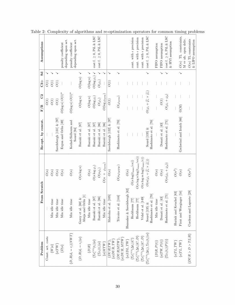
Table 2: Complexity of algorithms and re-optimization operators for common timing problems

Pro

ble

mFro

mScra

tch

Re-o

pt.

by

con

cat.

F/B

C2

C3+

Sd

Ass

um

pti

on

s

Con

st.

act.

cost

s—

O(n

)—

O(1

)O

(1)

X

W|ø

Min

idle

tim

eO

(n)

—O

(1)

O(1

)X

ø|TW

Min

idle

tim

eO

(n)

Sav

elsb

ergh

[131

]&

[97]

O(1

)O

(1)

X

D|ø

Min

idle

tim

eO

(n)

Erg

un

and

Orl

in[4

9]O

(logn

)O

(1)*

—p

enalt

yco

effici

ent

dep

endin

gup

on

act

.

D,R

(di

=r i

)|NWT

Min

idle

tim

eO

(n)

Ked

ad-S

idh

oum

and

Sou

rd[9

4]O

(logn

)O

(1)*

—p

enalt

yco

effici

ent

dep

endin

gup

on

act

.

D,R

(di

=r i

)|ø

Gar

eyet

al.

[60]

&A

hu

jaan

dO

rlin

[1]

O(n

logn

)Ib

arak

iet

al.

[87]

O(l

ogn

)O

(logn

)X

D|R

Min

idle

tim

eO

(n)

Ibar

aki

etal

.[8

7]O

(logn

)O

(logn

)X

Σcc

vx

i(ti)|ø

Ibar

aki

etal

.[8

7]

O(n

logϕc)

Ibar

aki

etal

.[8

7]O

(logϕc)

O(l

ogϕc)X

cost

f.≥

0,P

iL&

LSC

Σc i

(ti)|ø

Ibar

aki

etal

.[8

6]

O(nϕc)

Ibar

aki

etal

.[8

6]O

(ϕc)

O(ϕ

c)

Xco

stf.≥

0,P

iL&

LSC

ø|M

TW

Min

idle

tim

eO

(n+

ϕmtw

)Ib

arak

iet

al.

[86]

O(l

ogϕmtw

)—

X

DUR|TW,

ø|DUR,TW

Mal

colm

etal.

[105

]O

(n)

Sav

elsb

ergh

[132

]&

[97]

O(1

)O

(1)

X

DUR|M

TW,

ø|DUR,M

TW

Tri

coir

eet

al.

[144

]O

(nϕMTW

)H

ash

imot

oet

al.

[70]

O(ϕ

mtw

)—

X

ø|IDL,TW

Hu

nsa

ker

&S

avel

sber

gh[8

2]O

(n)

——

——

Σcc

vx

i(∆t i

)|C

Hoch

bau

m[7

7]O

(nlo

g(tmax/εn

))—

——

—co

nt.

wit

hε

pre

cisi

on

Σcc

vx

i(∆t i

)|C,D

Hoch

bau

m[7

7]O

(nlo

gn

log(tmax/εn

))—

——

—co

nt.

wit

hε

pre

cisi

on

Σcc

vx

i(∆t i

)|C,D

Vid

alet

al.

[149

]O

(nlo

gm

log(tmax/ε

))—

——

—co

nt.

wit

hε

pre

cisi

on

Σcc

vx

i(∆t i

),Σc i

(ti)|ø

Sou

rd[1

35]

&H

ash

imot

oet

al.

[70]

O(n

(ϕc

+ϕc×ϕc))

Sou

rd[1

35]

&H

ash

imot

oet

al.

[70]

O(ϕ

c+ϕc×ϕc)

—X

cost

f.≥

0,P

iL&

LSC

D|R,P

(t)

Min

idle

tim

eO

(n)

——

——

FIF

Oass

um

pti

on

ø|TW,P

(t)

Don

ati

etal

.[4

3]O

(n)

Don

ati

etal

.[4

3]O

(1)

—X

FIF

Oass

um

pti

on

Σc i

(ti)|P

(t)

Has

him

oto

etal

.[7

1]O

(n(ϕ

c+ϕp))

Has

him

oto

etal

.[7

1]O

(ϕc

+ϕp)

—X

cost

f.≥

0,P

iL&

LSC

&H

YI

ass

um

pti

on

ø|TL,TW

Hu

rin

kan

dK

euch

el[8

3]O

(n3)

——

——

ø|TL,TW

Fir

atan

dW

oeg

inge

r[5

4]O

(n)

Gsc

hw

ind

and

Irnic

h[6

6]O

(M)

——

XO

(n)

TL

const

rain

ts,

M⇔

nb.

op

endel

iv.

DUR>D>TL|R

Cor

dea

uan

dL

apor

te[2

9]O

(n2)

——

——

O(n

)T

Lco

nst

rain

ts&

LIF

Oass

um

pti

on

30

[4] M. Ayer, H.D. Brunk, G.M. Ewing, W.T. Reid, and E. Silverman. An empirical distributionfunction for sampling with incomplete information. The Annals of Mathematical Statistics, 26(4):641–647, 1955.

[5] K.R. Baker and G.D. Scudder. Sequencing with earliness and tardiness penalties: a review.Operations Research, 38(1):22–36, 1990.

[6] N. Balakrishnan. Simple heuristics for the vehicle routeing problem with soft time windows.Journal of the Operational Research Society, 44(3):279–287, 1993.

[7] R. Baldacci, A. Mingozzi, and R. Roberti. New route relaxation and pricing strategies for thevehicle routing problem. Operations Research, 59(5):1269–1283, 2011.

[8] R.E. Barlow, D.J. Bartholomew, J.M. Bremner, and H.D. Brunk. Statistical inference underorder restrictions: The theory and application of isotonic regression. Wiley New York, 1972.

[9] M. Bartusch, R.H. Mohring, and F.J. Radermacher. Scheduling project networks with resourceconstraints and time windows. Annals of Operations Research, 16(1):199–240, 1988.

[10] J.C. Bean, J.R. Birge, and R.L. Smith. Aggregation in dynamic programming. OperationsResearch, 35(2):215–220, 1987.

[11] J.E. Beasley. Adapting the savings algorithm for varying inter-customer travel times. Omega, 9(6):658–659, 1981.

[12] G. Berbeglia, J.-F. Cordeau, and G. Laporte. A hybrid tabu search and constraint programmingalgorithm for the dynamic dial-a-ride problem. INFORMS Journal on Computing, 24(3):343–355, 2012.

[13] D.P. Bertsekas, A. Nedi, and A.E. Ozdaglar. Nonlinear Programming. Athena Scientific, Nashua,NH, 2003.

[14] M.J. Best and N. Chakravarti. Active set algorithms for isotonic regression, a unifying frame-work. Mathematical Programming, 47(1-3):425–439, 1990.

[15] M.J Best, N. Chakravarti, and V.A. Ubhaya. Minimizing separable convex functions subject tosimple chain constraints. SIAM Journal on Optimization, 10(3):658–672, 2000.

[16] L. Bianco, A. Mingozzi, and S. Ricciardelli. The traveling salesman problem with cumulativecosts. Networks, 23(2):81–91, 1993.

[17] A. Blum, P. Chalasani, D. Coppersmith, B. Pulleyblank, P. Raghavan, and M. Sudan. Theminimum latency problem. In Proceedings of the twenty-sixth annual ACM symposium on Theoryof computing, pages 163–171, New York, USA, 1994. ACM.

[18] O. Braysy and M. Gendreau. Vehicle routing problem with time windows, Part II : Metaheuris-tics. Transportation Science, 39(1):119–139, 2005.

[19] O. Braysy and M. Gendreau. Vehicle routing problem with time windows, Part I : Routeconstruction and local search algorithms. Transportation Science, 39(1):104–118, 2005.

[20] P. Brucker, T. Hilbig, and J. Hurink. A branch and bound algorithm for a single-machinescheduling problem with positive and negative time-lags. Discrete Applied Mathematics, 94(1-3):77–99, 1999.

[21] H.D. Brunk. Maximum likelihood estimates of monotone parameters. The Annals of Mathemat-ical Statistics, 26(4):607–616, 1955.

[22] A.M. Campbell and M. Savelsbergh. Efficient insertion heuristics for vehicle routing and schedul-ing problems. Transportation science, 38(3):369–378, 2004.

[23] N. Chakravarti. Isotonic median regression: a linear programming approach. Mathematics of

31

Operations Research, 14(2):303–308, 1989.

[24] A. Charnes and W.W. Cooper. The theory of search: optimum distribution of search effort.Management Science, 5(1):44–50, 1958.

[25] T Cheng. A concise survey of scheduling with time-dependent processing times. EuropeanJournal of Operational Research, 152(1):1–13, 2004.

[26] P. Chretienne and F. Sourd. PERT scheduling with convex cost functions. Theoretical ComputerScience, 292(1):145–164, 2003.

[27] M. Christiansen and K. Fagerholt. Robust ship scheduling with multiple time windows. NavalResearch Logistics, 49(6):611–625, 2002.

[28] K.L. Cooke and E. Halsey. The shortest route through a network with time-dependent internodaltransit times. Journal of Mathematical Analysis and Applications, 14:493–498, 1966.

[29] J.-F. Cordeau and G. Laporte. A tabu search heuristic for the static multi-vehicle dial-a-rideproblem. Transportation Research Part B: Methodological, 37(6):579–594, 2003.

[30] J.-F. Cordeau, G. Laporte, and A. Mercier. A unified tabu search heuristic for vehicle routingproblems with time windows. Journal of the Operational Research Society, 52(8):928–936, 2001.

[31] J.-F. Cordeau, G. Laporte, and A. Mercier. Improved tabu search algorithm for the handlingof route duration constraints in vehicle routing problems with time windows. Journal of theOperational Research Society, 55(5):542– 546, 2004.

[32] R. Cordone. A note on time windows constraints in routing problems. Technical report, Depart-ment of Electronics and Information, Polytechnic of Milan, 2000.

[33] G.B. Dantzig. A control problem of Bellman. Management Science, 17(9):542–546, 1971.

[34] J.S. Davis and J.J. Kanet. Single-machine scheduling with early and tardy completion costs.Naval Research Logistics, 40:85–101, 1993.

[35] R. Dechter, I. Meiri, and J. Pearl. Temporal constraint networks. Artificial Intelligence, 49:61–95, 1991.

[36] E. Demir, T. Bektas, and G. Laporte. An adaptive large neighborhood search heuristic for thepollution-routing problem. European Journal of Operational Research, 223(2):346–359, 2012.

[37] G. Desaulniers and D. Villeneuve. The shortest path problem with time windows and linearwaiting costs. Transportation Science, 34(3):312–319, 2000.

[38] G. Desaulniers, J. Desrosiers, I. Ioachim, M.M. Solomon, F. Soumis, and D. Villeneuve. A unifiedframework for deterministic time constrained vehicle routing and crew scheduling problems. InT.G. Crainic and G. Laporte, editors, Fleet Management and Logistics, pages 129–154. KluwerAcademic Publishers, Boston, MA, 1998.

[39] G. Desaulniers, J. Desrosiers, and M.M. Solomon, editors. Column generation. Springer, 2005.

[40] M. Desrochers, J.K. Lenstra, and M.W.P. Savelsbergh. A classification scheme for vehicle routingand scheduling problems. European Journal of Operational Research, 46(3):322–332, 1990.

[41] M. Desrochers, J. Desrosiers, and M. Solomon. A new optimization algorithm for the vehiclerouting problem with time windows. Operations Research, 40(2):342–354, 1992.

[42] J. Desrosiers, Y. Dumas, M.M. Solomon, and F. Soumis. Time constrained routing and schedul-ing. In M. Ball, T. L. Magnanti, C.L. Monma, and G.L. Nemhauser, editors, Network Routing,pages 35–139. North-Holland Amsterdam, 1995.

[43] A. Donati, R. Montemanni, N. Casagrande, A.E. Rizzoli, and L.M. Gambardella. Time depen-dent vehicle routing problem with a multi ant colony system. European Journal of Operational

32

Research, 185(3):1174–1191, 2008.

[44] S.E. Dreyfus. An appraisal of some shortest-path algorithms. Operations Research, 17(3):395–412, 1969.

[45] C. Duhamel. Un Cadre Formel pour les Methodes par Amelioration Iterative - Application adeux problemes d’Optimisation dans les reseaux. PhD thesis, Universite Blaise Pascal, Clermont-Ferrand, 2001.

[46] Y. Dumas, F. Soumis, and J. Desrosiers. Optimizing the schedule for a fixed vehicle path withconvex inconvenience costs. Transportation Science, 24(2):145–152, 1990.

[47] M.E. Dyer and J. Walker. An algorithm for a separable integer programming problem withcumulatively bounded variables. Discrete applied mathematics, 16:135–149, 1987.

[48] I. Elhallaoui, D. Villeneuve, F. Soumis, and G. Desaulniers. Dynamic aggregation of set-partitioning constraints in column generation. Operations Research, 53(4):632–645, 2005.

[49] O. Ergun and J. Orlin. Fast neighborhood search for the single machine total weighted tardinessproblem. Operations Research Letters, 34(1):41–45, 2006.

[50] E. Erkut and J. Zhang. The maximum collection problem with time-dependent rewards. NavalResearch Logistics, 43(5):749–763, 1996.

[51] H. Everett. Generalized Lagrange multiplier method for solving problems of optimum allocationof resources. Operations Research, 11(3):399–417, 1963.

[52] D. Feillet, P. Dejax, and M. Gendreau. Traveling salesman problems with profits. TransportationScience, 39(2):188–205, 2005.

[53] G. Feng and H.C. Lau. Efficient algorithms for machine scheduling problems with earliness andtardiness penalties. Annals of Operations Research, 159(1):83–95, 2007.

[54] M. Firat and G.J. Woeginger. Analysis of the dial-a-ride problem of Hunsaker and Savelsbergh.Operations Research Letters, 39(1):32–35, 2011.

[55] M. Fischetti, G. Laporte, and S. Martello. The delivery man problem and cumulative matroids.Operations Research, 41(6):1055–1064, 1993.

[56] B. Fleischmann, M. Gietz, and S. Gnutzmann. Time-varying travel times in vehicle routing.Transportation Science, 38(2):160–173, 2004.

[57] A. Frangioni and A. Manca. A computational study of cost reoptimization for min-cost flowproblems. INFORMS Journal on Computing, 18(1):61–70, 2006.

[58] G.N. Frederickson and D.B. Johnson. The complexity of selection and ranking in X + Y andmatrices with sorted columns. Journal of Computer and System Sciences, 24(2):197–208, 1982.

[59] M.L. Fredman. On computing the length of longest increasing subsequences. Discrete Mathe-matics, 11(1):29–35, 1975.

[60] M.R. Garey, R.E. Tarjan, and G.T. Wilfong. One-processor scheduling with symmetric earlinessand tardiness penalties. Mathematics of Operations Research, 13(2):330–348, 1988.

[61] M. Gendreau and C.D. Tarantilis. Solving large-scale vehicle routing problems with time win-dows: The state-of-the-art. Technical report, CIRRELT, 2010.

[62] B. Giffler and G.L. Thompson. Algorithms for solving production-scheduling problems. Opera-tions Research, 8(4):487–503, 1960.

[63] S. Goto and A. Sangiovanni-Vincentelli. A new shortest path updating algorithm. Networks, 8(4):341–372, 1978.

33

[64] R.L. Graham, E.L. Lawler, J.K. Lenstra, and A.H.G Rinnooy Kan. Optimization and approxi-mation in deterministic sequencing and scheduling: a survey. Annals of Discrete Mathematics,5:287–326, 1979.

[65] S.J. Grotzinger and C. Witzgall. Projections onto order simplexes. Applied Mathematics andOptimization, 270(12):247–270, 1984.

[66] T. Gschwind and S. Irnich. Effective handling of dynamic time windows and synchronizationwith precedences for exact vehicle routing. Technical report, Johannes Gutenberg University,Mainz, Germany, 2012.

[67] J. Halpern. Shortest route with time dependent length of edges and limited delay possibilitiesin nodes. Zeitschrift fur Operations Research, 21(3):117–124, 1977.

[68] R.F. Hartl, G. Hasle, and G.K. Janssens. Special issue on rich vehicle routing problems. CentralEuropean Journal of Operations Research, 14(2):103–104, 2006.

[69] H. Hashimoto. Studies on local search-based approaches for vehicle routing and scheduling prob-lems. PhD thesis, Kyoto University, 2008.

[70] H. Hashimoto, T. Ibaraki, S. Imahori, and M. Yagiura. The vehicle routing problem with flexibletime windows and traveling times. Discrete Applied Mathematics, 154(16):2271–2290, 2006.

[71] H. Hashimoto, M. Yagiura, and T. Ibaraki. An iterated local search algorithm for the time-dependent vehicle routing problem with time windows. Discrete Optimization, 5(2):434–456,2008.

[72] H. Hashimoto, M. Yagiura, S. Imahori, and T. Ibaraki. Recent progress of local search inhandling the time window constraints of the vehicle routing problem. 4OR, 8(3):221–238, 2010.

[73] D. Haugland and S.C. Ho. Feasibility testing for dial-a-ride problems. In B. Chen, editor,Algorithmic Aspects in Information and Management, volume 6124 of LNCS, pages 170–179.Springer Berlin / Heidelberg, 2010.

[74] Y. Hendel and F. Sourd. Efficient neighborhood search for the one-machine earliness-tardinessscheduling problem. European Journal of Operational Research, 173(1):108–119, 2006.

[75] Y. Hendel and F. Sourd. An improved earliness-tardiness timing algorithm. Computers &Operations Research, 34(10):2931–2938, 2007.

[76] D. Hochbaum. Solving integer programs over monotone inequalities in three variables: A frame-work for half integrality and good approximations. European Journal of Operational Research,140(2):291–321, 2002.

[77] D.S. Hochbaum. Lower and upper bounds for the allocation problem and other nonlinear opti-mization problems. Mathematics of Operations Research, 19(2):390–409, 1994.

[78] D.S. Hochbaum and S.-P. Hong. About strongly polynomial time algorithms for quadraticoptimization over submodular constraints. Mathematical Programming, 69(1-3):269–309, 1995.

[79] D.S. Hochbaum and J.G. Shanthikumar. Convex separable optimization is not much harderthan linear optimization. Journal of the ACM (JACM), 37(4):843–862, 1990.

[80] J.A. Hoogeveen and S.L. Van De Velde. A branch-and-bound algorithm for single-machineearliness-tardiness scheduling with idle time. INFORMS Journal on Computing, 8(4):402–412,1996.

[81] H.H. Hoos and T. Stutzle. Stochastic local search: Foundations and applications. MorganKaufmann, 2005.

[82] B. Hunsaker and M.W.P. Savelsbergh. Efficient feasibility testing for dial-a-ride problems. Op-

34

erations Research Letters, 30(3):169–173, 2002.

[83] J. Hurink and J. Keuchel. Local search algorithms for a single-machine scheduling problem withpositive and negative time-lags. Discrete Applied Mathematics, 112(1-3):179–197, 2001.

[84] L.M. Hvattum, I. Norstad, K. Fagerholt, and G. Laporte. Analysis of an exact algorithm for thevessel speed optimization problem. Networks, 62(2):132–135, 2013.

[85] T. Ibaraki and N. Katoh. Resource allocation problems: algorithmic approaches. MIT Press,Boston, MA, 1988.

[86] T. Ibaraki, S. Imahori, M. Kubo, T. Masuda, T. Uno, and M. Yagiura. Effective local searchalgorithms for routing and scheduling problems with general time-window constraints. Trans-portation Science, 39(2):206–232, 2005.

[87] T. Ibaraki, S. Imahori, K. Nonobe, K. Sobue, T. Uno, and M. Yagiura. An iterated local searchalgorithm for the vehicle routing problem with convex time penalty functions. Discrete AppliedMathematics, 156(11):2050–2069, 2008.

[88] S. Ichoua, M. Gendreau, and J.Y. Potvin. Vehicle dispatching with time-dependent travel times.European Journal of Operational Research, 144(2):379–396, 2003.

[89] I. Ioachim, S. Gelinas, F. Soumis, and J. Desrosiers. A dynamic programming algorithm for theshortest path problem with time windows and linear node costs. Networks, 31(3):193–204, 1998.

[90] S. Irnich. A unified modeling and solution framework for vehicle routing and local search-basedmetaheuristics. INFORMS Journal on Computing, 20(2):270–287, 2008.

[91] S. Irnich. Resource extension functions: properties, inversion, and generalization to segments.OR Spectrum, 30:113–148, 2008.

[92] N. Karmarkar. A new polynomial-time algorithm for linear programming. Combinatorica, 4(4):373–395, 1984.

[93] W. Karush. A general algorithm for the optimal distribution of effort. Management Science, 9(1):50–72, 1962.

[94] S. Kedad-Sidhoum and F. Sourd. Fast neighborhood search for the single machine earliness-tardiness scheduling problem. Computers & Operations Research, 37(8):1464–1471, 2010.

[95] J.E. Kelley and M.R. Walker. Critical-path planning and scheduling. In Proceedings of Easternjoint Computer conference, pages 160–173, New York, 1959. ACM Press.

[96] L.G. Khachiyan. A polynomial algorithm in linear programming. Soviet Mathematics Doklady,20:191–194, 1979.

[97] G.A.P. Kindervater and M.W.P. Savelsbergh. Vehicle routing: Handling edge exchanges. InE.H.L. Aarts and J.K. Lenstra, editors, Local Search in Combinatorial Optimization, pages 337–360. Princeton Univ Pr, 1997.

[98] M.S. Kodialam and H. Luss. Algorithms for separable nonlinear resource allocation problems.Operations Research, 46(2):272–284, 1998.

[99] A.L. Kok, E.W. Hans, and J.M.J. Schutten. Vehicle routing under time-dependent travel times:the impact of congestion avoidance. Technical report, University of Twente, 2009.

[100] Y.A. Koskosidis, W.B. Powell, and M.M. Solomon. An optimization-based heuristic for vehiclerouting and scheduling with soft time window constraints. Transportation Science, 26(2):69–85,1992.

[101] C.Y. Lee and J.Y. Choi. A genetic algorithm for job sequencing problems with distinct duedates and general early-tardy penalty weights. Computers & Operations Research, 22(8):857–

35

869, 1995.

[102] H. Luss and S.K. Gupta. Allocation of effort resources among competing activities. OperationsResearch, 23(2):360–366, 1975.

[103] C. Malandraki and M.S. Daskin. Time dependent vehicle routing problems: Formulations,properties and heuristic algorithms. Transportation Science, 26(3):185–200, 1992.

[104] C. Malandraki and R.B. Dial. A restricted dynamic programming heuristic algorithm for thetime dependent traveling salesman problem. European Journal of Operational Research, 90(1):45–55, 1996.

[105] D.G. Malcolm, J.H. Roseboom, C.E. Clark, and W. Fazar. Application of a technique for researchand development program evaluation. Operations Research, 7(5):646–669, 1959.

[106] E. Miller-Hooks and B. Yang. Updating paths in time-varying networks given arc weight changes.Transportation Science, 39(4):451–464, 2005.

[107] L.G. Mitten. Sequencing n jobs on two machines with arbitrary time lags. Management Science,5(3):293–298, 1959.

[108] Y. Nagata. Effective memetic algorithm for the vehicle routing problem with time windows: Edgeassembly crossover for the VRPTW. In Proceedings of the Seventh Metaheuristics InternationalConference, Montreal, Canada (on CD-ROM), 2007.

[109] Y. Nagata, O. Braysy, and W. Dullaert. A penalty-based edge assembly memetic algorithmfor the vehicle routing problem with time windows. Computers & Operations Research, 37(4):724–737, 2010.

[110] S.U. Ngueveu, C. Prins, and R. Wolfler Calvo. An effective memetic algorithm for the cumulativecapacitated vehicle routing problem. Computers & Operations Research, 37(11):1877–1885, 2010.

[111] I. Norstad, K. Fagerholt, and G. Laporte. Tramp ship routing and scheduling with speed opti-mization. Transportation Research Part C: Emerging Technologies, 19(5):853–865, 2011.

[112] I. Or. Traveling salesman-type combinatorial problems and their relation to the logistics ofregional blood banking. PhD thesis, Northwestern University, Evanston, IL, 1976.

[113] A. Padakandla and R. Sundaresan. Power minimization for CDMA under colored noise. IEEETransactions on Communications, 57(10):3103–3112, 2009.

[114] S. Pallottino. A new algorithm for reoptimizing shortest paths when the arc costs change.Operations Research Letters, 31(2):149–160, 2003.

[115] Y. Pan and L. Shi. Dual constrained single machine sequencing to minimize total weightedcompletion time. IEEE Transactions on Automation Science and Engineering, 2(4):344–357,2005.

[116] P.M. Pardalos and G. Xue. Algorithms for a class of isotonic regression problems. Algorithmica,23(3):211–222, 1999.

[117] P.M. Pardalos, G.-L. Xue, and L. Yong. Efficient computation of an isotonic median regression.Applied Mathematics Letters, 8(2):67–70, 1995.

[118] S.N. Parragh, J.-F. Cordeau, K.F. Doerner, and R.F. Hartl. Models and algorithms for theheterogeneous dial-a-ride problem with driver-related constraints. OR Spectrum, 34(3):593–633,2012.

[119] M. Patriksson. A survey on the continuous nonlinear resource allocation problem. EuropeanJournal of Operational Research, 185(1):1–46, 2008.

[120] D.W. Pentico. The assortment problem: A survey. European Journal of Operational Research,

36

190(2):295–309, 2008.

[121] M. Pinedo. Scheduling: theory, algorithms, and systems. Prentice Hall, 2008.

[122] C.N. Potts and J.D. Whitehead. Heuristics for a coupled-operation scheduling problem. Journalof the Operational Research Society, 58(10):1375–1388, 2007.

[123] J.-Y. Potvin and J.-M. Rousseau. An exchange heuristic for routeing problems with time win-dows. Journal of the Operational Research Society, 46(12):1433–1446, 1995.

[124] E. Prescott-Gagnon, G. Desaulniers, and L.M. Rousseau. A branch-and-price-based large neigh-borhood search algorithm for the vehicle routing problem with time windows. Networks, 54(4):190–204, 2009.

[125] G. Righini and M. Salani. Symmetry helps: Bounded bi-directional dynamic programming forthe elementary shortest path problem with resource constraints. Discrete Optimization, 3(3):255–273, 2006.

[126] T. Robertson, F.T. Wright, and R.L. Dykstra. Order Restricted Statistical Inference. WileySeries in Probability and Statistics. John Wiley & Sons, New York, 1988.

[127] R.T. Rockafellar. Convex analysis. Princeton Univ Press, 1970.

[128] B. Roy. Contribution de la theorie des graphes a l’etude de certains problemes lineaires. Comptesrendus de l’academie des sciences de Paris, 248:2437–2439, 1959.

[129] B. Roy. Graphes et ordonnancement. Revue Francaise de Recherche Operationnelle, 25:323–333,1962.

[130] L. Sanathanan. On an allocation problem with multistage constraints. Operations Research, 19(7):1647–1663, 1971.

[131] M.W.P. Savelsbergh. Local search in routing problems with time windows. Annals of OperationsResearch, 4(1):285–305, 1985.

[132] M.W.P. Savelsbergh. The vehicle routing problem with time windows: Minimizing route dura-tion. ORSA Journal on Computing, 4(2):146–154, 1992.

[133] T.R. Sexton and L.D. Bodin. Optimizing single vehicle many-to-many operations with desireddelivery times: I. Scheduling. Transportation Science, 19(4):378–410, 1985.

[134] T.R. Sexton and L.D. Bodin. Optimizing single vehicle many-to-many operations with desireddelivery times: II. Routing. Transportation Science, 19(4):411–435, 1985.

[135] F. Sourd. Optimal timing of a sequence of tasks with general completion costs. European Journalof Operational Research, 165(1):82–96, 2005.

[136] F. Sourd and S. Kedad-Sidhoum. The one-machine problem with earliness and tardiness penal-ties. Journal of Scheduling, 6(6):533–549, 2003.

[137] K.S. Srikantan. A problem in optimum allocation. Operations Research, 11(2):265–273, 1963.

[138] W. Szwarc and S.K. Mukhopadhyay. Optimal timing schedules in earliness-tardiness singlemachine sequencing. Naval Research Logistics, 42(7):1109–1114, 1995.

[139] M. Tagmouti, M. Gendreau, and J.-Y. Potvin. Arc routing problems with time-dependent servicecosts. European Journal of Operational Research, 181(1):30–39, 2007.

[140] E. Taillard, P. Badeau, M. Gendreau, F. Guertin, and J.-Y. Potvin. A tabu search heuristicfor the vehicle routing problem with soft time windows. Transportation Science, 31(2):170–186,1997.

[141] F.B. Talbot. Resource-constrained project scheduling with time-resource tradeoffs: the nonpre-

37

emptive case. Management Science, 28(10):1197–1210, 1982.

[142] A. Tamir. Efficient algorithms for a selection problem with nested constraints and its applicationto a production-sales planning model. SIAM Journal on Control and Optimization, 18(3):282–287, 1980.

[143] J. Tang, Y. Kong, H. Lau, and A.W.H. Ip. A note on “Efficient feasibility testing for dial-a-rideproblems”. Operations Research Letters, 38(5):405–407, 2010.

[144] F. Tricoire, M. Romauch, K.F. Doerner, and R.F. Hartl. Heuristics for the multi-period orien-teering problem with multiple time windows. Computers & Operations Research, 37(2):351–367,2010.

[145] T. Van Woensel, L. Kerbache, H. Peremans, and N. Vandaele. Vehicle routing with dynamictravel times: a queueing approach. European Journal of Operational Research, 186(3):990–1007,2008.

[146] T. Vidal, T.G. Crainic, M. Gendreau, and C. Prins. Heuristics for multi-attribute vehicle routingproblems: a survey and synthesis. European Journal of Operational Research, 231(1):1–21, 2013.

[147] T. Vidal, T.G. Crainic, M. Gendreau, and C. Prins. A hybrid genetic algorithm with adaptivediversity management for a large class of vehicle routing problems with time-windows. Computers& Operations Research, 40(1):475–489, 2013.

[148] T. Vidal, T.G. Crainic, M. Gendreau, and C. Prins. Time-window relaxations in vehicle routingheuristics. Technical report, CIRRELT, Montreal, 2013.

[149] T. Vidal, P. Jaillet, and N. Maculan. A decomposition algorithm for nested resource allocationproblems. Technical report, MIT, Cambridge, 2014.

[150] C. Walshaw. A multilevel approach to the travelling salesman problem. Operations Research,50(5):862–877, 2002.

[151] G. Wan and B.P.-C. Yen. Tabu search for single machine scheduling with distinct due windowsand weighted earliness/tardiness penalties. European Journal of Operational Research, 142(2):271–281, 2002.

[152] C.A. Yano and Y.-D. Kim. Algorithms for a class of single-machine weighted tardiness andearliness problems. European Journal of Operational Research, 52(2):167–178, 1991.

Appendix

A Reduction of LISP to TW (unit)|PGiven a vector N = (N1, . . . , Nn) of n real numbers, LISP aims to find the maximum length L of anon-decreasing subsequence of numbers: L = maxk|1 ≤ i1 < · · · < ik ≤ n and Ni1 ≤ · · · ≤ Nik.From a LISP instance, we construct the following instance T of TW (unit)|ø, with n activities suchthat for i ∈ 1, . . . , n, ri = di = Ni and pi = 0. This instance is created in n elementary algorithmicoperations.

Let z∗(T ) be the optimal solution cost of T . This solution naturally initiates as many activitiesas possible without penalties, within a non-decreasing order of execution dates. Hence, the activitiesachieved without penalty correspond to the LISP subsequence sought in the original problem, whoselength is L∗ = n − z∗(T ). Hence, LISP admits a many-one reduction to TW (unit)|ø. Conversely,TW (unit)|ø generalizes LISP.

38

B Proof of Theorem 1: Block optimality conditions of Σccvxi (ti)|ø

We first recall the corresponding timing problem, stated in Equations (64-65).

min(t1,...,tn)∈<n

n∑i=1

ci(ti) (64)

s.t. ti + pi ≤ ti+1 1 ≤ i < n (65)

The functions ci(t) : < → < are assumed to be convex, but not necessarily smooth. We denoteby δci(t) the subdifferential of ci at t, which is necessarily a non-empty interval, as a byproductof the convexity assumption and the space of definition. We first recall two useful properties onsubdifferentials from Rockafellar [127], to follow with the proof of Theorem (1).

Proposition 2. Let f1, . . . , fm be subdifferentiable functions on <n, then:

δ(f1(x) + · · ·+ fm(x)) ⊃ δf1(x) + · · ·+ δfm(x) ∀x (66)

Theorem 2. Let f1, . . . , fm be a set of proper convex functions on <n having at least one commonpoint in the relative interior of their domains ri(dom(fi)), then:

δ(f1(x) + · · ·+ fm(x)) = δf1(x) + · · ·+ δfm(x) ∀x ∈⋂ri(dom(fi)) (67)

Constraint qualifications hold as the constraints are linear, and any solution with idle time betweeneach activity is feasible, thus taking place in the relative interior of the polytope. Hence, strong dualityapplies, leading to the following necessary and sufficient optimality conditions. A solution t∗ =(t∗1, . . . , t

∗n) of Problem (64-65) is optimal if and only if a set of Lagrangian multipliers (λ∗1, . . . , λ

∗n−1)

exists, such that conditions (68) are satisfied (Bertsekas et al. 13, Propositions 5.7.1 and 6.4.2).

t∗i−1 + pi−1 ≤ t∗i i = 2, . . . , n

0 ∈ δc1(t∗1) + λ∗1

0 ∈ δci(t∗i ) + λ∗i − λ∗i−1 i = 2, . . . , n− 1

0 ∈ δcn(t∗n)− λ∗n−1

λ∗i−1(t∗i−1 + pi−1 − t∗i ) = 0 i = 2, . . . , n

λ∗i ≥ 0 i = 1, . . . , n

(68)

Solution t∗ can be represented as a succession of blocks of activities (B1, . . . , Bm), such thatactivities within each block are processed without idle time, and the last activities of blocks are followedby non-zero idle time. The previous definition, combined with primal feasibility, yields t∗Bj(|Bj |) +

pBj(|Bj |) < t∗Bj(|Bj |)+1, and thus λ∗Bj(|Bj |) = 0 for j ∈ 1, . . . ,m − 1. Conditions (68) are thus

equivalent to primal feasibility (equivalent to the first condition of (1) combined with the definition ofblocks) and the following independent systems of equations for each block:

∀j ∈ 1, . . . ,m

i) 0 ∈ δcBj(1)(t∗Bj(1)) + λ∗Bj(1)

ii) 0 ∈ δci(t∗Bj(1) + pBj(1)i−1) + λ∗i − λ∗i−1 i = Bj(1) + 1, . . . , Bj(|Bj |)− 1

iii) 0 ∈ δcBj(|Bj |)(t∗Bj(1) + pBj(1)Bj(|Bj |−1)))− λ∗Bj(|Bj |)−1

iv) λ∗i ≥ 0 i = Bj(1), . . . , Bj(|Bj |)(69)

39

Necessary condition proof. For 1 ≤ i ≤ j ≤ n, let pij be the cumulative processing duration ofactivities ai to aj . Relying on Proposition (2), one can sum i) , ii) and iii) of (69), leading to:

0 ∈ δcBj(1)(t∗Bj(1)) +

Bj(|Bj |)∑i=Bj(1)+1

δci(t∗Bj(1) + pBj(1)i−1)⇒ 0 ∈ δCBj (t∗Bj(1)) , (70)

and thus, following the definition of the optimal block execution cost of Equation (18), t∗Bi(1) ∈[T−∗Bi , T

+∗Bi

]. Any optimal solution thus verifies the first statement of Theorem (1). Finally, for any

block Bj and prefix block Bkj , summing i) , ii) and iii) for j ∈ Bj(1) + 1, . . . , k leads to:

− λ∗k ∈ δcBj(1)(t∗Bj(1)) +

k∑i=Bj(1)+1

δci(t∗Bj(1) + pBj(1)i−1)⇒ −λ∗k ∈ δCBj (t∗Bkj (1)

) , (71)

which can be reformulated as T+∗Bkj≥ t∗Bj(1) and implies the last statement of Theorem (1).

Sufficient condition proof. Consider a solution t = (t1, . . . , tn) with its blocks (B1, . . . , Bm),respecting conditions of Theorem (1). Following block definitions and primal feasibility, it only remainsto prove that Conditions (69) are respected for each block. We choose the following Lagrangianmultipliers, which are non-negative as T+∗

Bki≥ tBi(1) ⇒ ∃x ≤ 0 ∈ δCBij (tBj(1))):

∀j ∈ 1, . . . ,m

λ∗i = −min(x ∈ δCBij (tBj(1))) i = Bj(1) + 1, . . . , Bj(|Bj |)− 1

λ∗Bj(|Bj |) = 0(72)

Proposition (2) then involves that for i ∈ 1, . . . ,m and j ∈ Bj(1) + 1, . . . , Bj(|Bj |)− 1;

− λ∗i ∈ δCBij (tBj(1)) = δcBj(1)(tBj(1)) +i∑

k=Bj(1)+1

δck(tBj(1) + pBj(1)k−1) (73)

In the case where i = Bj(1), Equation (73) proves statement i) of (69). Also, λ∗Bj(1) ∈ δ(−cBj(1))(tBj(1)),

and we can combine this statement with Equation (73) for i = Bj(1)+1, using Proposition 2), leadingto:

λ∗Bj(1)+1 − λ∗Bj(1) ∈ δ(−cBj(1))(tBj(1)) + δcBj(1)(tBj(1)) + δcBj(1)+1(tBj(1) + pBj(1))

= δcBj(1)+1(tBj(1) + pBj(1))(74)

The remaining statements of Equation ii) and Equation iii) in (69) are proven by recurrence.Assuming that for a given i ∈ Bj(1) + 1, . . . , Bj(|Bj |)− 1, λ∗i−1 − λ∗i ∈ δci(tBj(1) + pBj(1)i), then

λ∗i − λ∗i+1 = −λ∗i+1 + λ∗i−1 − (λ∗i−1 − λ∗i )

∈ δcBj(1)(tBj(1)) +

i+1∑k=Bj(1)

δck(tBj(1) + pBj(1)k−1) + δ(−cBj(1))(tBj(1))

+i−1∑

k=Bj(1)

δ(−ck)(tBj(1) + pBj(1)k−1) + δ(−ci)(tBj(1) + pBj(1)i−1)

⊂ δci+1(tBj(1) + pBj(1)i)

(75)

All the sufficient optimality conditions are thus satisfied by solution t = (t1, . . . , tn). ut

40