This article was downloaded by: [Universite Laval]On: 10 October 2014, At: 10:04Publisher: Taylor & FrancisInforma Ltd Registered in England and Wales Registered Number: 1072954Registered office: Mortimer House, 37-41 Mortimer Street, London W1T 3JH, UK

Astronomical & AstrophysicalTransactions: The Journal of theEurasian Astronomical SocietyPublication details, including instructions for authors andsubscription information:http://www.tandfonline.com/loi/gaat20

Time series analysis of unequallyspaced data: Intercomparisonbetween the Schuster periodogramand the LS-spectraV. V. Vityazev aa Astronomy Department , St. Petersburg University ,Bibliotechnaya, pl. 2, Petrodvorets, St. Petersburg, 198904,RussiaPublished online: 17 Aug 2006.

To cite this article: V. V. Vityazev (1996) Time series analysis of unequally spaced data:Intercomparison between the Schuster periodogram and the LS-spectra, Astronomical &Astrophysical Transactions: The Journal of the Eurasian Astronomical Society, 11:2, 139-158,DOI: 10.1080/10556799608205461

To link to this article: http://dx.doi.org/10.1080/10556799608205461

PLEASE SCROLL DOWN FOR ARTICLE

Taylor & Francis makes every effort to ensure the accuracy of all the information(the “Content”) contained in the publications on our platform. However, Taylor& Francis, our agents, and our licensors make no representations or warrantieswhatsoever as to the accuracy, completeness, or suitability for any purpose of theContent. Any opinions and views expressed in this publication are the opinions andviews of the authors, and are not the views of or endorsed by Taylor & Francis. Theaccuracy of the Content should not be relied upon and should be independentlyverified with primary sources of information. Taylor and Francis shall not be liablefor any losses, actions, claims, proceedings, demands, costs, expenses, damages,and other liabilities whatsoever or howsoever caused arising directly or indirectly inconnection with, in relation to or arising out of the use of the Content.

This article may be used for research, teaching, and private study purposes. Anysubstantial or systematic reproduction, redistribution, reselling, loan, sub-licensing,systematic supply, or distribution in any form to anyone is expressly forbidden.

Terms & Conditions of access and use can be found at http://www.tandfonline.com/page/terms-and-conditions

Dow

nloa

ded

by [

Uni

vers

ite L

aval

] at

10:

04 1

0 O

ctob

er 2

014

Astronomical and Astrophysical Transactions, 1996, Vol. 11, pp. 139-158 Reprints available directly from the publisher Photocopying permitted by license only

0 1 9 9 6 OPA (Overseas Publishers Association) Amsterdam B.V. Published in The Netherlands

under license by Gordon and Breach Science Publishers SA

Printed in Malaysia

TIME SERIES ANALYSIS OF UNEQUALLY SPACED DATA: INTERCOMPARISON

BETWEEN THE SCHUSTER PERIODOGRAM AND THE LS-SPECTRA

V. V. VITYAZEV

Astronomy Department, St. Petersburg University, Babliotechnaya, p l . 2, Petrodvorets, St. Petersburg, 198904, Russia

(Received November 9, 2995)

At present, the Schuster periodogram and the LS-spectra are widely used for evaluating the power spectra of irregularly spaced time series. According to many authorities, the LS-spectra are prefer- able over the Schuster periodogram since they are based on the least-squares fitting of a sine function to the data and since they have the exponential distribution when the time series is pure noise. On the other hand, the practice of spectral analysis shows that the Schuster periodogram and the LS-spectra often are almost identical. In this paper the theoretical study of all the esti- mators is made with the purpose to describe the situations when the Schuster periodogram differs from the LS-spestra sufficiently. It is shown that the likeness of the periodograms under consid- eration depends on the properties of the spectral window W ( w ) corresponding to the distribution of time points. The main results are: a) all the estimators evaluated at frequency w are identical if W ( 2 w ) = 0; b) the Schuster periodogram differs from the LS-spectra at the frequency w = 0 / 2 , where ij is the frequency at which the spectral window has a large side peak due to irregular distribution of time points. The numerical examples for several situations typical in astronomy illustrate these conclusions.

KEY WORDS Power spectra, time series

1 INTRODUCTION

In various branches of astronomy, we face the problem of finding unknown period- icities hidden in the observational data. If data are regularly spaced in time, the Discrete Fourier Transform (DFT) and the Schuster periodogram associated with it (Schuster, 1898) are the basic tools for evaluating the power spectra (Jenkins and Watts, 1968; Otnes and Enocson, 1978; Marple, 1987; Terebizh, 1992, etc.). Unfortunatly, the astronomical observations are irregular due to different reasons: day-time changes, weather conditions, positions of the object under observations

139

Dow

nloa

ded

by [

Uni

vers

ite L

aval

] at

10:

04 1

0 O

ctob

er 2

014

140 V. V. VITYAZEV

and so on. The present day theory and practice of the spectral analysis of the un- equally spaced time series are based on two approaches. The first one employs the Schuster periodogram for unequally spaced data (Deeming, 1975a, 1975b; Roberts et al., 1987). The second one uses the procedure of the least-squares fitting of a sinusoid to the data (Barning, 1962; Lomb, 1976; Ferraz-Mello, 1981, Scargle, 1982, 1989). The resulting estimators (the so-called LS-spectra) and the modified discrete Fourier transforms associated with them are widely used nowadays. The most valu- able feature of the LS-spectra is their well-defined statistical behavior. At the same time, the LS-spectra lose several very important properties: they cannot be dis- cribed in terms of the spectral window, they cannot be strictly connected with the correlation function, etc. On the other hand, the Schuster periodogram of a gapped time series satisfies all the fundamental relations of the classical spectral analysis, but its statistical properties are complicated as compared to the case of regular data. It is worth mentioning that, despite different theoretical foundations, the Schuster periodogram and the LS-spectra frequently turn out to be almost identical. This similarity requires an explanation, and this is the main point of the present pa- per in which we are trying to find situations when the Schuster periodogram and the LS-spectra are very close to each other or differ greatly. The final goal of this study is to clarify the properties of various techniques which are used to derive the periodicities in the unequally distributed data.

2 THE LEAST-SQUARES PROCEDURE AS AN ESTIMATOR OF THE POWER SPECTRUM

We begin by exposing the general least-squares approach that produces various kinds of the LS-spectra. Given a set of N observations

2 k = z ( t k ) , k = 0, 1,. . . , N - 1

with zero mean obtained at arbitrary times t k , we can set up the model

2

i= l

where 4l ( t ) = cos w t ,

&(t) = sin w t .

Defining the residuals of approximation as

we can find the coefficients al and 0 2 from the condition

Dow

nloa

ded

by [

Uni

vers

ite L

aval

] at

10:

04 1

0 O

ctob

er 2

014

SCHUSTER PERIODOGRAM AND LS-SPECTRA 141

where the following notation is used:

llP1I2 = (P,P). (2.7) In our case the coefficients a1 and a2 are determined as the solution of the corre- sponding normal equations:

(2.8)

where A = 1141112114112 - ( 4 1 9 4 2 ) .

Now, for the quantity ~ , , , i ” = [1e1l2 = min

(2.9)

(2.10)

one has 2

Emin = 1 1 ~ 1 1 ~ - C a i ( Z , 4i). (2.11) i=l

If the functions 41 and 4 2 are orthogonal, then

(2.12)

Consider now the function

P(w) = 112112 - Emin 2 0. (2.13)

Obviously, the function P(w), when plotted against w , will have sharp peaks if a trial frequency coincides with the frequency of the model (2.1). For this reason, the function P(w) may be used as an estimator of the power spectrum. Following Lomb (1976), we call this estimator the LS-spectrum. Its final representation is

(2.14)

The factor !j is introduced for convenience of comparison befween the LS-spectrum and the Schuster periodogram.

3 THE TYPES OF THE LS-SPECTRA

It is a common practice to use the term “periodogram” to designate an estimator of the power spectrum. In this sense, the various types of the LS-spectra considered in this paper will be called periodograms with the names of their authors.

Dow

nloa

ded

by [

Uni

vers

ite L

aval

] at

10:

04 1

0 O

ctob

er 2

014

142 V. V. VITYAZEV

3.1 The Baming Periodogram

Although the numerical least-squares algorithm was widely used to obtain the values of the 01 and a2 in spectral analysis of time series, it was Barning (1962) who first introduced the concept of the LS-spectrum and derived its analytical representation. In our notation, the expression for the Barning periodogram follows from Eqs. (2.8) and (2.14) in the form:

3.2 The Lomb Periodogram

To study the statistical properties of the LS-spectrum, it is desirable to have i t as a sum of two squared functions. This can be done by several methods. One of them was proposed by Lomb (1976). His approach is based on the introduction of the new time points

f k = tk - T(W), (3-2)

where the time shift 1 & sin 2wtk

~ ( w ) = -arctan 2u c k cos 2wtk

provides the orthogonality of the functions

(3.3)

Under this assumption the Lomb periodogram looks as follows:

1 2

L(w) = -

Following this idea, Scargle (1982, Fourier transform:

1989) introduced a specific kind of the discrete

1 FT(w) = - exp(-iwto)

4 in terms of which the Lomb periodogram becomes

L(w) = IFT(w)12.

+ i-) 6 2

114211 ' (3.7)

Dow

nloa

ded

by [

Uni

vers

ite L

aval

] at

10:

04 1

0 O

ctob

er 2

014

SCHUSTER PERIODOGRAM AND LS-SPECTRA 143

9.3 The Ferraz-Mello Periodogram

Another method to express the periodogram as a sum of two squared quantities was proposed by Ferraz-Mello (1981). His approach is based on representing the data by orthogonal functions $0 , $1, $2 which can be derived from the initial functions 1, 41, 4 2 by means of the Gram-Schmidt procedure. Obviously, this method corresponds to a “sinusoid plus constant” model. To simplify discussion and to make the results comparable to the “sinusoid” model which is the cornerstone in the Barning’s and the Lomb’s techniques, we shall apply the orthogonalization procedure to our functions 41, 4 2 . The corresponding orthogonalized functions are:

$1 = 41,

(41 9 4 2 ) dl, * a = 4 2 - - 114111

(41,h) ’

ll4lll2 l1*a1l2 = 1142 -

The final expression for the Ferraz-Mello periodogram looks as follows:

or 1 2

F M ( U ) = - I D C D F T ( ~ ) ~ ~ ,

where

(3.9)

(3.10)

(3.11)

(3.12)

(3.13)

(3.14)

(3.15)

is a new type of transform (the Date-Compensated Discrete Fourier Transform).

4 THE SCHUSTER PERIODOGRAM

In our notation, this “classical” estimator of the power spectrum can be written in the form

This expression shows that if the signal contains a sine function of frequency W O ,

then the product xke-iwtk makes a large contribution to S provided that w = W O .

In other words, the Schuster periodogram, to the limit of normalizing factor, is a square of the correlation coefficient between the data and a harmonic function. Thus we see that the Schuster periodogram differs from the LS-spectra by definition. It

Dow

nloa

ded

by [

Uni

vers

ite L

aval

] at

10:

04 1

0 O

ctob

er 2

014

144 V. V. VITYAZEV

is likely that due to the correlation nature, the Schuster periodogram and the true power spectrum G(w) of the function

~ ( t ) = A cos (wot + 40) (4.2)

are connected by the next

S(w)

where

relation (Vityazev, 1994):

= T G ( w ) W ( w - u') dw' + SO(W), --M

(4.3)

W(w) = IQ(w)l?

Henceforth, the functions Q(w) and W ( w ) will be referred to as t h e cornplez spectral window and the spectral window, respectively. A set of functions given by Eq. (4.2), with phases 40, randomly distributed within the interval [0,27r], may be regarded as a stationary stochastic process. Averaging Eq. (4.4) over the set of realizations yields (SO) = 0, thus reducing Eq. (4.2) to a convolution of the true spectrum G ( w ) with the spectral window W(w). This result was obtained by Deeming (1975), who studied the Schuster periodogram averaged over the realizations, given at the same set of arbitrary time points. It is very important to emphasize that the transition from G ( w ) to S(w) is completely explained by the spectral window W ( w ) . In particular, the convolution term in Eq. (4.3) reveals all the artifacts introduced into the periodogram by missing points (Deeming, 1975; Vityazev, 1994). Thus we see that the spectral windows, depending only on the distribution of time points, are very useful tools in spectral analysis, and we shall use them intensively in the next sections.

5 THE SCHUSTER PERIODOGRAM AND THE LS-SPECTRA

In this section we compare our periodograms. At first, the intercomparison between the LS-spectra is made.

Theorem 1. For any time series given at arbitrary time points, the Ferraz- Mello periodograrn and the Barning periodogram are identical.

To prove this theorem, we write the obvious relations that can be obtained from Eqs. (3.9)-( 3.12) :

(2,111) = (2 , Ol), (5.1)

Dow

nloa

ded

by [

Uni

vers

ite L

aval

] at

10:

04 1

0 O

ctob

er 2

014

SCHUSTER PERIODOGRAM AND LS-SPECTRA 145

11~111211~2112 = 11411121142112 - (41 1 4d2. (5.3) Now, the identity FM(w) = B(w) follows from Eq. (3.13), if Eqs, (5.1)-(5.3) are taken into consideration.

Theorem 2. For any time series given at arbitrary time points, the Lomb periodogram and the Barning periodogram are identical.

To prove this theorem, we shall use the relations:

(z,&) = Cr(z, 41) + ST(z, 4 2 ) ,

( 2 1 6 2 ) = Cr(z, $2) - sT(z, 411, (5-4)

(5.5) where

C, = cos w r , S, = sin w r . It is not difficult to show that

(5.7)

ReR(2w) cos 2wr = d m l ImR(2w)

d W ' sin 2wr =

(5.9)

(5.10)

Substitution of Eqs. (5.5)-(5.10) into Eq. (3.6) gives the identity L(w) = B(w) if the relation

11~111211i2112 = 11411121142112 - (41,42)2 = 1 - W(2w) (5.11)

is taken into account. Now we see that different expressions which define the Barning, the Lomb, and

the Ferraz-Mello periodograms give one and the same result, and thus the general name for them - the LS-spectrum - is justified.

In order to compare the Schuster periodogram with the LS-spectrum, we rewrite Eq. (3.1) in the form:

where (5.13)

(5.14)

(5.15)

Dow

nloa

ded

by [

Uni

vers

ite L

aval

] at

10:

04 1

0 O

ctob

er 2

014

146

Suppose that

V. V. VITYAZEV

(5.16)

ReQ(2w) = 0, (5.17)

and, consequently, W(2w) = 0. (5.18)

In this case, the right-hand sides of Eqs. (4.1) and (5.12) coincide, and we come to the main conclusion of the present paper:

A t the set of frequencies that satisfy Eq. (5.18), the Schuster periodogram and the LS-spectra are identical, otherwise they difler, and the closer to zero i s the valve 1 - W(2w), the stronger i s their diflerence.

Thus we see that the degree of likeness between the Schuster periodogram and the LS-spectra depends on the structure of the spectral window. In the next section we shall demonstrate several important distributions of time points for which the frequencies that satisfy Eq. (5.18) do exist.

Theorem 3.

6 THE SPECTRAL WINDOWS FOR TYPICAL DISTRIBUTIONS OF TIME POINTS

As we have seen, the key problem in the intercomparison between the spectra es- timators is the study of the spectral windows. For any set of time points, the numerical calculation of the spectral windows can be done without problems. In this section we consider some typical distributions of points for which the spectral windows have analytical representations.

6.1 The Regular T i m e Series

In this case the sequence of time points is

t k = A t k , k = O , 1 , ..., N - 1 , (6-1)

where At is a constant interval. For simplicity we consider N as an even number. The analytical forms of the spectral windows are known to be

sin2 ( N w At /2) N 2 sin2(wAt/2) ’ W ( W ) WO(W, N , At) =

sin (NwAt/2) N sin (wAt/2)

R e O ( w ) = COS((N - l ) ~ A t / 2 ) ,

sin( NwAtl2) N sin(wAt/2) ImQ(w) = sin((N - l)wAt/2).

Dow

nloa

ded

by [

Uni

vers

ite L

aval

] at

10:

04 1

0 O

ctob

er 2

014

SCHUSTER PERIODOGRAM AND LS-SPECTRA 147

Usually, the Schuster periodogram is evaluated a t the set of natural frequencies

27r . . N NAt 2

Wj=-J , J=O, l , . . . , --1.

It is easy to verify that W(2Wj) = 0.

This gives us the first real example of a time points distribution, when the frequen- cies that satisfy Eq. (5.18) do exist. Now, we can conclude: in the case of regular observations the Schuster periodogram and the LS-spectra are identical provided their values are calculated at the natural frequencies (6.5).

6.2

The astronomical observations are often performed with periodic or quasi-periodic gaps. Ground-based observations are interrupted by day-night alteration giving gaps with the 24-hour period; the meteorological changes for a given site are re- peated annually; the observations from a space vehicle are usually stopped when the satellite enters the radiation belts. To make a model of time points distributed with periodical gaps, we suppose that, in the set of regular observations with a constant sampling interval At, one has n succesive observations and p succesive missing points, and the group of n + p points is repeated m times. In this case the period of gaps is AT = (n+p)At . In the previous papers (Vityazev, 1994; Vityazev and Prudnikiva, 1994) we have shown that in this case the spectral window looks as follows:

Time Series with Periodic Gaps

W(W) = WO(TW, At)Wo(m,w, AT), (6.7)

where Wo is given by Eq. (6.2). Due to gaps in observations, the spectral window W(w) has well-pronounced side peaks at the proper frequencies

- 2 s W I = 1, 1 = 1 , 2 , . . . , ( n + p)/2.

m(n + p)At

If in our set of m(n + p ) points all the missing points all are filled in, then we can introduce the set of natural frequencies

27r j, j = 1,2, . . . , m(n + p)/2. W ' - - m(n + p)At

Excluding from w, the values w,/2, we'form a new set of frequencies:

27r m(n+p)At

wf = j, j = 1,2 , . . . ,m/2-1, m/2+1,. . , m - l , m + l , . . . , m(n+p)/2-1,

(6.10) which satisfy Eq. (5.18). This gives us reason to state that when the frequency of gaps is 6 1 = 27r/T, the Schuster periodogram and the LS-spectra calculated at the

Dow

nloa

ded

by [

Uni

vers

ite L

aval

] at

10:

04 1

0 O

ctob

er 2

014

2.1

= u

-

1.3

- 0.5

-2

-0.3

-O

0 0

0

mo

o

00

0

o

80

0

OO

0

00

O

O

oo

o

o

80

0

0

OO

-1.1

-1

.9 -

I 0,

-

"I

I

I n

E

0.0

2.8

5.7

8.5

11.4

14.2

0.00

1.00

2.00

ma

4.00

5.00

Tim

e, fsl

freq

uen

cy,

Il

A

1.00

0

0.75

9 -

0.51

9-

0.278-

b

-0.203

0.037 -

1 J,- I

I I

MirJ

dulu

s of

Spec

tral

win

dow

1.

om

0.800

0.600

IM

of

Spec

tral

win

dow

0.703

I I

-0.4

28

I I

I I

I

0.00

1.00

2.00

3.00

4.00

5.00

0.00

1.00

2.00

3.00

4.00

5.00

Fre

qu

ency

, f 1

/sI

Fre

qu

ency

, C I/sl

Fig

ure

1

Fun

ctio

ns W

(u),

ReR(w), a

nd I

niR

(w)

for

the

set

of t

ime

poin

ts w

ith p

erio

dic gaps (

n =

3; p

= 7; m

= 1

5).

Dow

nloa

ded

by [

Uni

vers

ite L

aval

] at

10:

04 1

0 O

ctob

er 2

014

€ 3 L c U 01 0 VI I m A

E a L U 0 U 0 .A L at n L a8 UI 3 L U u)

Y

SCHUSTER PERIODOGRAM AND LS-SPECTRA

- = + s

4

Dow

nloa

ded

by [

Uni

vers

ite L

aval

] at

10:

04 1

0 O

ctob

er 2

014

150 V. V. VITYAZEV

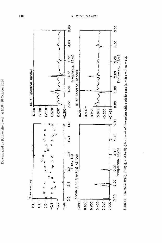
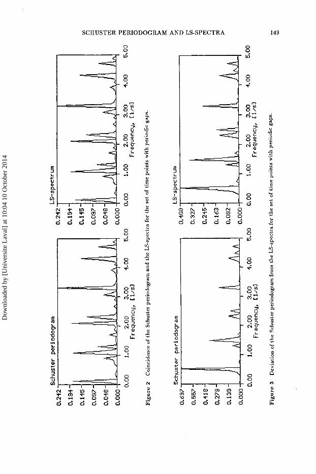
frequencies w; are the same, provided that the frequencies of the harmonics in the data do not coincide with the values wl/2. Figure 1 shows the time series

~ ( t ) = A1 C O S ( ~ T V ~ ~ ) + A2 C O S ( ~ T V ~ ~ ) , (6.11)

generated a t the time points with periodical gaps ( n = 3, p = 7, rn = 15, At = O.ls), and the functions W(w), ReR(w), and ImR(w), corresponding to this distribution of time points. We see that the side peaks are located a t the proper frequencies vl = 1, v2,. . . , v5 = 5. In Figure 2 we show the Schuster periodogram and the LS- spectrum, calculated for the parameters A1 = 1, A2 = 1, v1 = 1.1 Hz, v2 = 3.3 Hz. We see, that all the periodograms are identical, since no one of the values 214 and 2 ~ 2 coincides with the proper frequencies fi,, a t which W(.j) # 0. The opposite case is shown in Figure 3, where our periodograms were calculated for A1 = 1, A2 = 1, v1 = 0.5 Hz, v2 = 3.3 Hz. Now we have 2vl = fil = 1 Hz, that is why the Schuster periodogram drastically differs from the LS-spectrum.

6.3

Considered here is a situation when two sets of observations (each one consisting of n successive points) are separated by p missing points forming the gap. As earlier, all the points are supposed to be regularly spaced over the time interval At = const. Now, for the spectral window we have (Vityazev, 1994):

Observations with a Long Gap

W ( W ) W O ( ~ , W , At)[cOs((n + p)wAt)]/2.

It is not difficult to show that the frequencies

T 1 w t = ( j + T ) , j = O , l , . . . , n + p - 1 , ( n + p ) A t

(6.12)

(6.13)

satisfy the condition (6.6). It is important to note that the proper frequencies of the spectral window (6.12) defined as

- 2 s W k = k, k = 1 , 2 ,...,

(n + P l a t (6.14)

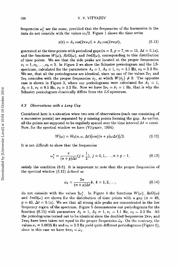
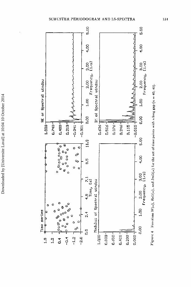
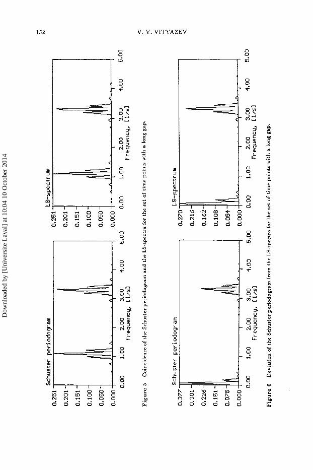
do not coinside with the values 2w* In Figure 4 the functions W(w) , ReQ(w) and I m n ( w ) are shown for the distribution of time points with a gap (n = 40, p = 40, At = 0.1s). We see that all strong side peaks are concentrated in the low frequency region of the spectrum. Figure 5 demonstrates our periodograms for the function (6.11) with parameters A1 = 1, A2 = 1, v1 = 1.1 Hz, vz = 3.3 Hz. All the periodograms turned out to be identical since the doubled frequenvies 2nu1 and 2 7 ~ 2 have been taken not equal to the proper frequencies GI. On the contrary, the values v1 = 0.0625 Hz and v2 = 3.3 Hz yield quite different periodograms (Figure S), since in this case we have 4TU1 = G1.

J :

Dow

nloa

ded

by [

Uni

vers

ite L

aval

] at

10:

04 1

0 O

ctob

er 2

014

3 0 f3 c 3

r(l

U aJ

m 0

.d

.-I

L c

n

.t

SCHUSTER PERIODOGRAM AND LS-SPECTRA

u 4 .-I

c3

u 9

151

Dow

nloa

ded

by [

Uni

vers

ite L

aval

] at

10:

04 1

0 O

ctob

er 2

014

152

E 3

U QI 0 u1 I

(I]

L c

V. V. VITYAZEV

b"

4 ~

L + c C U I

U -

0 9

0

R 0 B

Dow

nloa

ded

by [

Uni

vers

ite L

aval

] at

10:

04 1

0 O

ctob

er 2

014

SCHUSTER PERIODOGRAM AND LS-SPECTRA 153

w

O I

0 0

0 0

go J

O0 0

L4

% o o

0

0

0 0

0 0 0

0

%lo

0 0 0

0

0 I ' 0 , q 1

i

Dow

nloa

ded

by [

Uni

vers

ite L

aval

] at

10:

04 1

0 O

ctob

er 2

014

154 V. V. VITYAZEV

Schuster periodogram 0.292

0.234 - 0.175 - 0.117-

0.058 - 0.000

r

8 - v A I I I 1

0.00 1.00 2.00 3.00 4.00 5.00 Frequency, f l / d

LS-spect r um

0.174

0.116

0.00 1.00 2.00 3.00 4.00 5.00 Frequency, I: l/sl

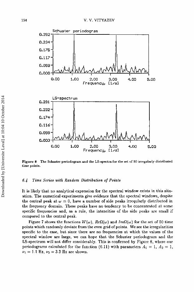
Figure 8 time points.

The Schuster periodogam and the LS-spectra for the set of 50 irregularly distributed

6.4 Tame Series with Random Distribution of Points

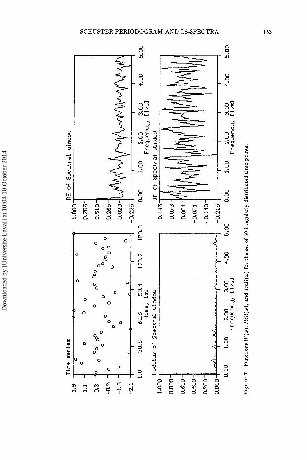
It is likely that no analytical expression for the spectral window exists in this situ- ation. The numerical experiments give evidence that the spectral windows, despite the central peak at w = 0, have a number of side peaks irreqularly distributed in the frequency domain. These peaks have no tendency to be concentrated at some specific frequencies and, as a rule, the intencities of the side peaks are small if compared to the central peak.

Figure 7 shows the functions W ( w ) , ReQ(w) and IrnQ(w) for the set of 50 time points which randomly deviate from the even grid of points. We see the irregularities specific to the case, but since there are no frequencies at which the values of the spectral window are large, we can hope that the Schuster periodogram and the LS-spectrum will not differ considerably. This is confirmed by Figure 8, where our periodograms calculated for the function (6.11) with parameters A1 = 1, A2 = 1, v1 = 1.1 Hz, v2 = 3.3 Hz are shown.

Dow

nloa

ded

by [

Uni

vers

ite L

aval

] at

10:

04 1

0 O

ctob

er 2

014

SCHUSTER PERIODOGRAM AND LS-SPECTRA 155

7 MIXTURE OF PERIODICITIES

As we have seen, at the frequencies defined by Eq. (5.18) all the periodograms under consideration are identical. In this section the opposite case is studied, that is, we try to answer the question: what happens when we have the condition

1 - W(2w) << 1. (7.1)

First of all, let us write the expressions which show the intensity of the peak centered a t W O , where w o is the frequency of a sine function given by Eq. (4.2). For the Schuster periodogram, from Eqs. (4.3) and (4.4) we have:

A2 A2 A2

4 2 ~ ( w o ) = -[1+ W ( ~ W O ) ] + -ReR(2wo)cos 240 - -ImR(2wo)sin 2 240, (7.2)

where 40 is the phase of the sine fuction. The analogous equation valid for the LS-spectrum looks as follows:

(7.3) A2 4 B(wo) = -[1+ ReR(2wo) cos 240 - ImR(2wo) sin 2401.

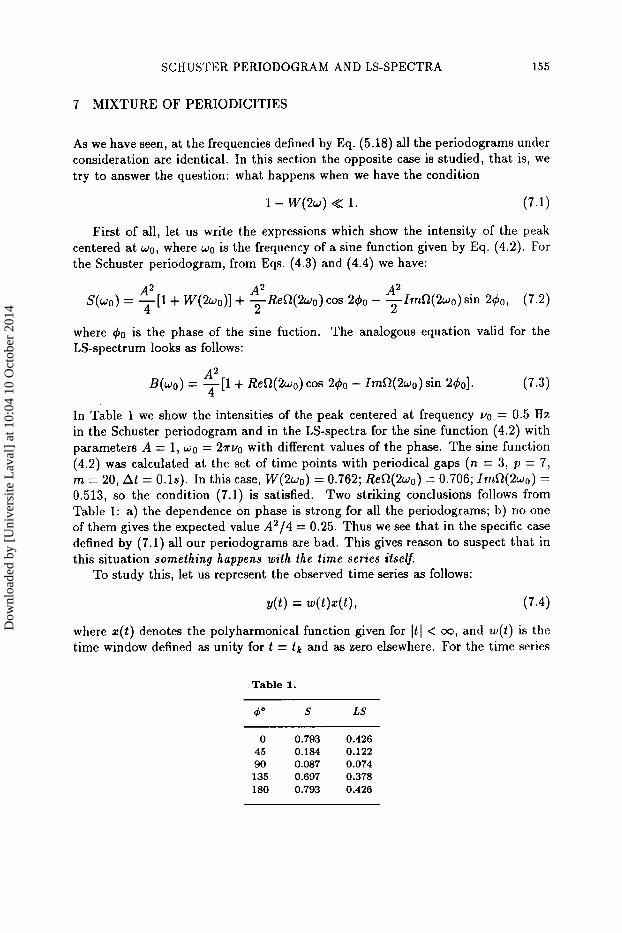
In Table 1 we show the intensities of the peak centered at frequency vo = 0.5 Hz in the Schuster periodogram and in the LS-spectra for the sine function (4.2) with parameters A = 1, w o = 2 ~ ~ 0 with different values of the phase. The sine function (4.2) was calculated at the set of time points with periodical gaps ( n = 3, p = 7 , m = 20, At = 0.1s). In this case, W(2wo) = 0.762; ReR(2wo) = 0.706; ImR(2wo) = 0.513, so the condition (7.1) is satisfied. Two striking conclusions follows from Table 1: a) the dependence on phase is strong for all the periodograms; b) no one of them gives the expected value A2/4 = 0.25. Thus we see that in the specific case defined by (7.1) all our periodograms are bad. This gives reason to suspect that in this situation something happens wiih the time series itself.

To study this, let us represent the observed time series as follows:

Y O ) = w(t>z(t>, (7.4)

where z ( t ) denotes the polyharmonical function given for It I < 00, and w(t) is the time window defined as unity for t = tk and as zero elsewhere. For the time series

Table 1.

do S LS ~~~~~~~ ~

0 0.793 0.426 45 0.184 0.122 90 0.087 0.074 135 0.697 0.378 180 0.793 0.426

Dow

nloa

ded

by [

Uni

vers

ite L

aval

] at

10:

04 1

0 O

ctob

er 2

014

156 V. V. VITYAZEV

with periodic gaps, considered in Subsection 6.2, the time window can be replaced by its Fourier series:

52

w(t) = a 0 + c YI cos(G1t + 4r), (7.5) 1=1

where wl are the proper frequencies defined by (6.8). If the function z( t ) is given by Eq. (4.2), then we have:

y(t) = aoA cos(wot + 40)

The power spectrum of this function consists of lines (of peaks, when the peri- odogram analysis is used) a t the frequencies f w o that correspond to the signal and lines at IWI f w0I which are usually called “the ghosts”, i.e. false lines due to gaps in observations. In the case of periodic gaps, the ghosts follow each other with the unterval Aw = = 27r/AT. If 2w0 # w l , then the ghosts of the true lines located at f w o do not interfere. Otherwise, they coincide and change the intensities of the lines. This is clearly seen in the time domain too, for if we put wo = W1/2, then Eq. (7.6) yields

where

A ” 2 + - c y1 COS[(Wl - wo)t + 41 - 401,

1=2 (7.7)

P1 = y1/2ao. (7.9)

Comparison between Eqs. (4.2) and (7.7) shows that the observations with periodic gaps change the amplitude and the phase of the initial signal. It is true that, due to the rectangular form of the function w(t), the Fourier series (7.5) converges to 3 (not to 1) at the first and the nth points in each segment of n + p points. For this reason, Eqs. 7.4 and 7.6 coincide everywhere except these points. Nevertheless, this defect of convergence does not play a crucial role in our analysis, and our main conclusion is: if a harmonic process of frequency wo i s observed with periodic gaps of frequency 2w0, then the observed lime series becomes a mixture of these two periodic

Dow

nloa

ded

by [

Uni

vers

ite L

aval

] at

10:

04 1

0 O

ctob

er 2

014

SCHUSTER PERIODOGRAM A N D LS-SPECTRA 157

processes. We would obtain the same results each time when the condi€ion (7.1) is satisfied. In such pathological situations, the estimation of the power spectrum will be wrong, no m a t t e r what es t imator (from those considered in this paper) is used.

8 CONCLUSIONS

The results of this study may be summarized as follows: a) all the LS-spectra considered in this paper - the Barning, the Lomb, and the Ferraz-Mello periodograms (based on the pure sinusoid model) - are identical; b) the likeness between the Schuster periodogram and the LS-spectra is governed by the behavior of the spectral window; c) a t those frequencies where W ( 2 w ) = 0, all the periodograms under consideration are identical. d ) if the maxima of the spectral window (except the central peak) are small, then all the periodograms are nearly identical; e) the Schuster periodogram differs from the LS-spectra only at the frequencies that satisfy the condition 1 - W ( 2 w ) << 1. It means that the discrepancies between the Schuster periodogram and the LS-spectra are large when the time series contain a harmonic of the frequency, the double value of which coincides with the frequency at which the spectral window has a large side peak. In the case of periodical gaps, it happens when the period of a signal hidden in the data is one half the period of the gaps. In this pathological situation, the spectral estimation faces unrealistic intensities of the spectral peaks and the strong dependence of the hights of peaks on the phase of the signal. It is very important to emphasize that these problems come not from the choise of the periodogram-the problems are hard for all the periodgrams that we have studied-but they originate from mixing two sources of the periodicities: one is the physical process that we observe and another one is a periodical interruption of observations. In astronomy, the rotation and revolution of the Earth impose diurnal and annual cycles on the Earth-based observations. The periods hidden in observations of the Sun, stars, quasars, etc., are hardly connected physically with the periods specific to the Earth. For these observations, the probability to come across the mixing of the periodicities is negligible. On the contrary, if we study the Earth from the Earth (such is the case with the astrometric observations of the Earth's rotation parameters), then the semi-annual period known in the Earth rotation interferes with the annual gaps in observations.

Nevertheless, exept for pathological situations, the Schuster periodogram is prac- tically identical to the LS-spectra. This forces us to to make a closer examination of the statistical properties of the Schuster periodogram for uneven time series. And this is a topic for the next article.

References

Barning,F. J. M., (1962) B.A.N. 17, No. 1, 22. Deeming, T. J. (1975a) Astrophys. Space Sci. 36, 137.

Dow

nloa

ded

by [

Uni

vers

ite L

aval

] at

10:

04 1

0 O

ctob

er 2

014

158 V. V. VITYAZEV

Deeming, T. J. (1975b) Astrophys. Space Sci. 42, 257(E). Ferraz-Mello, S. (1981) Astron. J . 86, 619. Jenkins, G. M. and Watts, D. G. (1968) Spectral analysis and its applications, Holden-Day, San

Lomb, N. R. (1976) Astrophys. Space Sci. 39, 447. Marple, Jr., S. L. (1987) Digital Spectral Analysis wi th Applications, Prentice-Hall, Englewood

Otnes, R. K. and Enocson, L. (1978) Applied T i m e Series Analysis, A Wiley-Interscience Publi-

Roberts, D. H., Lehar, J., and Dreher, J. W. (1987) Astron. J . 93, 968. Scargle, J. D. (1982) Astrophys. J. 263, 835. Scargle, J. D. (1989) Astrophys. J . 343, 874. Schuster, A. (1898) Terrestrial Magnet ism 3, 13. Terebish V. Yu. (1992) T i m e Series Analysis in Astrophysics, Moscow, Nauka. Vityasev, V. V. (1994) Astron. and Astrophys. Tr . 5 , 177. Vityasev, V. V. and Prudnikova, E. Ya. (1994) Vestn. S t . Peteraburg clniv., Ser. 1, issue 2, No. 8 ,

Francisco.

Cliffs, New Jersey.

cation, New York.

78.

Dow

nloa

ded

by [

Uni

vers

ite L

aval

] at

10:

04 1

0 O

ctob

er 2

014