time dependent modelling and simulation of the …707884/fulltext01.pdf · degree project time...

Degree project

Time Dependent Modelling and Simulation of the Corona Discharge in Electrostatic Precipitators

Authors: Eduard Potrymai, Ivan Perstnov Supervisor: Börje Nilsson Examiner: Matz Lenells Date: 2014-03-25 Course Code: 5ED06E Subject: Electrical Engineering Level: Master Level Department Of Physics and Electrical Engineering

Abstract

Corona discharge is one of the crucial problems related with high-voltage equipment. Thispaper focuses on the physical and numerical modelling of corona discharge in an Elec-trostatic precipitator (ESP). The model is based on Maxwells equations and the Finiteelement method (FEM) and is implemented with the COMSOL Multiphysics software.The simulation allows studying the electric charge distribution and the behaviour of theelectric field inside the ESP. The work is focused primarily on time-dependent studies ofthe corona discharge.

Acknowledgements

This project is a result of collaboration between Linnaeus University and ALSTOM PowerSweden AB, therefore many professionals were involved to help us get into the topic anddo the best we can. It was a great honour and invaluable experience to work under thesupervision of all these people.

We want to thank our supervisor professor Borje Nilsson for helping us with wide rangeof problems and for his encouraging attitude and understanding. We would also like tothank professor Matz Lenells and supervisor from Alstom Per Ranstad for organizing thisproject for us and for ongoing support during our work as well as for making academicformalities easy for us.

We are grateful to Andreas Back and Joel Cramsky for giving us the starting point bysharing the results of their own work and experience and for invaluably useful practicaladvices during the work on the project. Our special thank goes to Leif Lindau whowillingly shared his great experience to improve the quality of the project.

Last but not the least, we want to thank our families and friends for their supportand understanding.

Contents

1 Introduction to ESP 4

2 Theoretical basics for modelling and simulation 72.1 Corona discharge theory and approximations . . . . . . . . . . . . . . . . 7

2.1.1 Mathematical model . . . . . . . . . . . . . . . . . . . . . . . . . 92.1.2 Boundary conditions . . . . . . . . . . . . . . . . . . . . . . . . . 11

2.2 Numerical methods overview . . . . . . . . . . . . . . . . . . . . . . . . . 122.2.1 The boundary element method (BEM) . . . . . . . . . . . . . . . 122.2.2 The method of characteristics (MOC) . . . . . . . . . . . . . . . . 122.2.3 The finite element method (FEM) . . . . . . . . . . . . . . . . . . 13

2.3 COMSOL Multiphysics . . . . . . . . . . . . . . . . . . . . . . . . . . . . 14

3 Modelling and simulation 153.1 Stationary analysis . . . . . . . . . . . . . . . . . . . . . . . . . . . . . . 15

3.1.1 Direct implementation of Peek-Kaptzov model . . . . . . . . . . . 163.1.2 Injection law-based modelling . . . . . . . . . . . . . . . . . . . . 18

3.2 Time-dependent analysis . . . . . . . . . . . . . . . . . . . . . . . . . . . 223.2.1 Current-controlled model . . . . . . . . . . . . . . . . . . . . . . . 233.2.2 Voltage-controlled model . . . . . . . . . . . . . . . . . . . . . . . 30

4 Conclusions and discussion 37

3

CHAPTER 1. INTRODUCTION TO ESP

Chapter 1

Introduction to ESP

The Electrostatic Precipitator (ESP) is a collecting device that removes different particles(such as dust and aerosols) from the gas flow using the force of the electric field [1]. It isusually designed as a set of metal plates with metal electrodes stretched between them.A potential difference of several kilovolts (in industrial installations up to several tens ofkilovolts) is created between the electrodes. The potential difference results in a strongelectric field between the electrodes and plates. On the surface of the electrode a coronadischarge occurs and in combination with the electric field it provides an ion current fromthe electrode to the plate. Polluted air is fed into the space between the plates. Dustparticles from the polluted air passing through the filter become charged (ionized) underthe influence of the ion current, and then get attracted to the plates and settle on them.

Figure 1.1: Overview of an Electrostatic precipitator [1].

The principle of operation of the Electrostatic Precipitator was proposed in 1824, andin 1907 Frederick Cottrell patented the first design.

ESPs continue to be excellent devices for control of many industrial particulate emis-sions, including flue gas from electricity-generating utilities (coal and oil fired). Elec-trostatic precipitators are generally able to remove more than 99% of the particles inexhaust, without having to force the air through a filter. They have lower pressure dropand therefore lower operating costs compared to fabric filters [2].

Setting up an ESP system is an expensive and complicated process. But what iseven more important is keeping the system effectively working for as long as possible

Page 4 of 40


(this period can last for 20-30 years). That is why the processes inside an ESP must bemonitored. The problem here is that only few parameters can be adjusted or measureddirectly. It is only the output of the power supply that can be adjusted; it is also possibleto measure the current on the plates. But this information in itself does not give thewhole picture of what is happening inside the ESP.

The way for solving this problem is to have a real time virtual model of an ESP. Itwould become possible to see how the real system behaves at this particular momentwhen a certain voltage (or current) is applied, how its state changes in time etc., just byusing the model with the same input parameters.

The separation of suspended particles from a flue gas by the electrostatic precipitationrequires three fundamental steps [3]:

� electrical charging of suspended particles,

� collection of the particles on the surface in an electric field,

� removal of the precipitated material from the collecting electrodes.

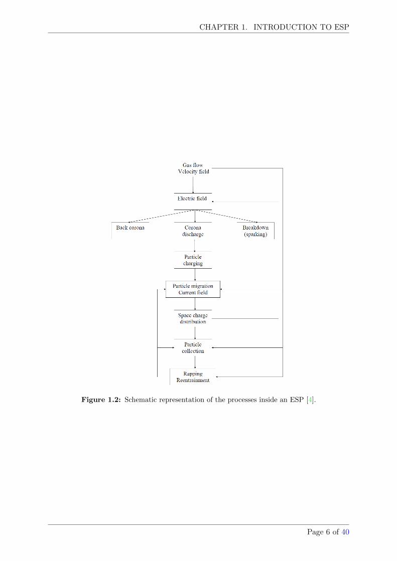
However, for a complete description of the process more details must be considered. Theexpanded scheme of the processes and the relations between them are given in Figure1.2 [4]. The blocks of the scheme can be expanded for including additional phenomenaor combined and avoided for simplification depending on the demands for a particularproblem. The mandatory step for building the model is the representation of the structure(geometry) of the ESP.

The goals of this work:

� Developing a model of the central process in ESP operation - the process of coronadischarge - and analysis of data received during simulations.

� Recreation of the stationary analysis models described in [5], [6], [7] and performingsimulation using COMSOL Multiphysics software.

� Improving and expansion of the existing methods of corona discharge analysis touse them for the time-dependent study of the process.

� Confirmation of the possibility of time-dependent analysis by means of modernhard- and software.

� Developing adequate models for time-dependent simulation as the first step towardsthe creation of real-time model of an ESP.

� One of the additional aims of the project is to develop the instructions for adaptationof the COMSOL Multiphysics software for the simulation of corona discharge inESPs.

Page 5 of 40


Figure 1.2: Schematic representation of the processes inside an ESP [4].

Page 6 of 40

Chapter 2

Theoretical basics for modelling and simula-tion

2.1 Corona discharge theory and approximations

The basic theory and assumptions for describing and modelling corona discharge givenin this section follow the book by H.J. White [3] unless other sources are stated.

Corona discharge is one of many forms of electrical conduction in gases. Electricalconductivity in gases differs from that in solids and liquids since gases normally containno free electrons or ions. However, the conductivity of the gas increases greatly when thepotential between the electrodes is high and the ionization occurs. The transition of gasfrom the insulating to conducting state is called an electric breakdown or gas discharge.

The main ionization mechanism in the corona discharge is the electron impact. Ac-cording to Townsend [8] the equation for electron ionization is

dn = αndx, (2.1)

where dn is the increase of the number of electrons produced by n electrons which passa distance element dx in the field. The coefficient α is a function of the field strengthand gas pressure and depends on the gas type. In the general case, when the field andtherefore α vary with x, the integration of (2.1) gives∫ x

0

dn

n=

∫ x

0

αdx (2.2)

orn = n0e

∫ x0 αdx. (2.3)

Another property of the electrons is their ability to attach to many molecular andatomic species. Negative gas ions are the result of the electrons attachment. The electronattachment is a probability phenomenon described by a survival equation

n = n0e−ηx, (2.4)

where η is a coefficient of attachment dependent both on the gas type and the electricfield. Combining ionization (2.3) and attachment (2.4) for non-uniform fields the valueof n becomes

n = n0e∫ x0 (α−η)dx. (2.5)

7

CHAPTER 2. THEORETICAL BASICS FOR MODELLING AND SIMULATION

The example of this situation is the negative corona in air. The electrons at thecorona wire generate many additional electrons because of large α and small η. Somegases have little or no affinity for electrons which means that electrons do not attach tothe molecules of these gases and their coefficient of attachment η is zero. It is obviousthat negative corona is impossible in gases with zero electron affinity.

Gas discharges may be divided into self-maintaining and nonself-maintaining [3] de-pending on the necessity of external ionization means for maintaining the process. Theunipolar corona (negative), used in electrical precipitation, is a stable, self-maintaininggas discharge between an emitting electrode and a plate.

The first studies about corona discharges started early in the 20th century as a detri-mental mode of breakdown in high voltage conductors.

The physical phenomena of corona discharge were carefully studied by Townsend[8], Loeb [9], Peek [10] and Kaptzov [11], both theoretically and empirically throughexperiments.

One of the most important gas discharge characteristics is the current voltage char-acteristic usually expressed in the form of a curve which shows the relation between thecurrent and the voltage.Warburg [12] (1899), working with point-plane electrodes, dis-covered the important parabolic relation between the corona current i and the voltage Uexpressed by

i = AU(U −M). (2.6)

A and M are experimentally determined constants. A similar relationship was foundto hold for concentric wire-and-cylinder electrodes by Almy [13] (1902). A theoreticalderivation of the parabolic equation was given by Towsend [8] for concentric cylinderelectrodes.

Since the time of early researches, corona discharges have been used for various appli-cations, such as electrostatic precipitation, ozone generation, ionic wind devices, nitrogenlaser, etc. Therefore, a comprehensive knowledge of all processes occurring in high voltageelectric fields is important for using these processes and phenomena in electrotechnicalapparatus.

Types of corona:

� Positive corona. The discharge is formed on the conductor, positively charged (e.g.,during the positive half-wave voltage). It is generally found in areas with sharpcorners. The visual appearance of this corona type is small region of a glow arounda certain location. This is a relatively weak source of corona discharge, and itcreates a slight sound.

� Negative corona. This type of corona typically occurs on the conductor, negativelycharged, for example, during the negative half-wave voltage. This type of coronalooks like a flame with constantly changing shape, direction and size. This coronais very sensitive to changes in the environmental parameters. Its appearance givesrise to an acoustic tone around the double-frequency (e.g. 100 Hz) of the electricfield or a multiple of it.

The second type of corona discharge is used in electrostatic precipitation.

Page 8 of 40


The main functions of electric field in ESPs can be divided into charging of parti-cles and controlling their movement trajectories. Corona discharge is one of the mostefficient ways to charge particles. The collecting devices use two forms of electrode sys-tems: ”needle-to-plane” and ”wire-to-plane”. The first is used when larger values of theelectric field strength, spatial charge density and electric wind velocity must be concen-trated in a small area, and the second where these quantities can be smaller, but moreevenly distributed in a wide area. In an electrostatic precipitator the second type of elec-trode system, ”wire-to-plane”, is often used. Therefore, in this work, the ”wire-to-plane”electrode system will be considered for future investigation.

The process of the electric corona discharge for an ESP includes the following factors:

� Applied voltage U between collecting plane and emitting electrode (wire);

� Electrical field E (described by the Poisson equation [14]);

� Ion space charge density, ρ;

� Fluid (moving gas, υair);

� Particle tracking, particle charge, ρparticle;

� Corona discharge.

2.1.1 Mathematical model

The mathematical model of the corona discharge has been derived under the followingassumptions:

� The emitting electrode is a smooth round wire, with the corona discharge uniformlydistributed over its surface;

� The Ion mobility is constant;

� The Thickness of the ionization layer can be neglected;

� The drift zone contains ions of one polarity;

� The electric field satisfies Kaptzov’s assumption [11] (explained in sec. 2.1.2).

The following set of equations for the electric field and the space charge densitydescribes the process of a unipolar corona discharge.

Maxwell’s equations are used as a basis [15]:

∇ · ε0E = ρ , (2.7)

∇ ·B = 0 , (2.8)

∇× 1

µ0

B = J +∂ε0E

∂t, (2.9)

Page 9 of 40


∇×E +∂B

∂t= 0, (2.10)

where ρ - space charge density, ε0 - electric permittivity µ0 - magnetic permeability, J -current density. Since the magnetic field B is divergence free it can be represented by avector potential A so that

B = ∇×A. (2.11)

The space charge ρ has to satisfy the charge conservation law. Taking the divergenceof (2.9) yields the continuity equation:

∂ρ

∂t+∇ · J = 0 . (2.12)

It now follows from Maxwell’s equations (2.10) that there exists a potential Φ so that

E = −∇Φ− ∂A

∂t. (2.13)

Assuming that ∂A/∂t is neglected in (2.13) the quasi stationary approximation can bemade for time-dependent case meaning that

E = −∇Φ. (2.14)

This is a low frequency approximation. Let a be a typical distance in the geometryand let c = (ε0µ0)−1/2 be the speed of light. Then a typical angular frequency is ω0 = c/aand a typical time is t0 = a/c. The quasi stationary approximation holds if the angularfrequency ω in E, which is the time Fourier transform of E, is much smaller than ω0 orthe time t after the source have been switched on is much larger than t0.

The combination of (2.7) and (2.14) gives the Poisson equation:

∇ ·E = ∇ · (−∇Φ) = −∇2Φ = ρ/ε0 ,

∇2Φ = −ρ/ε0. (2.15)

The current density J is assumed to be [16]

J = KρE + ρ υair −D∇ρ , (2.16)

where K is the mobility of the charge carriers, which depends on atmospheric pressureand room temperature. It can be taken as a constant equal to K = 1.8 ∼ 2.2 · 10−4 m2

Vs

[16]. D is a diffusion constant in the order of 10−5 m2

s[17]. Thus the system of two

coupled PDEs 2.12 and 2.15 with J given by 2.16 describes the physics of the process.

The current density equation (2.16) contains three components via ρ and φ: thedrift current KρE, the convection current ρυair, and the diffusion current −D∇ρ. Thetypical gas velocity is about 15m/s [3]. The drift velocity of the ions is approximatelyK · E ≈ 2 · 10−4 · 5 · 106 = 103m/s which is two orders of magnitude higher then the

Page 10 of 40


velocity of the gas flow. Neglecting or keeping the convective component creates twomodels of the corona discharge problem: decoupled and fully coupled models [16].

The decoupled model for the static case when

∇ · J = 0 (2.17)

is derived by combining (2.17) with (2.15) and (2.16):

∇ · J = ∇ · (KρE)−∇ · (D∇ρ) = 0

∇ · (KρE) = ∇ρ ·KE +Kρ(∇ ·E) = K((∇ρ)(−∇Φ) + ρ2/ε0

),

∇ · (D∇ρ) = D∇2ρ⇒

K(ρ2/ε0 −∇ρ · ∇Φ)−D∇2ρ = 0. (2.18)

Neglecting the diffusion current in (2.18) gives

∇ρ · ∇Φ = ρ2/ε0. (2.19)

The fully coupled model is derived the same way, but includes the convective current(diffusion current neglected for simplicity):

∇ · J = ∇ · (KρE) +∇ · (ρυair),

∇ρ · (KE) + ρ(∇ ·KE) +∇ρ · υair + ρ(∇ · υair) = 0,

ρ(∇ ·KE) = Kρ2

ε0

(2.15),∇ · υair = 0 (flow continuity [16]),

∇ρ(KE + υair) = −Kρ2/ε0. (2.20)

In this work the convective component is not considered and the diffusion componentis sometimes used for better numerical convergence.

2.1.2 Boundary conditions

The set of equations (2.14 - 2.20), represented above, is supplemented by the followingboundary conditions:

� The potential on the collecting plate is equal to zero;

� The potential on the emitting electrode is equal to the ESP’s operating voltage U ;

� The space charge density conditions are derived from Kaptzov assumption [11]: theelectric field on the emitting electrode increases proportionally to the voltage untila certain value, called the corona onset level Eon. After that the electrical field atthe injecting electrode remains unchanged and equal to the onset value Eon.

Page 11 of 40


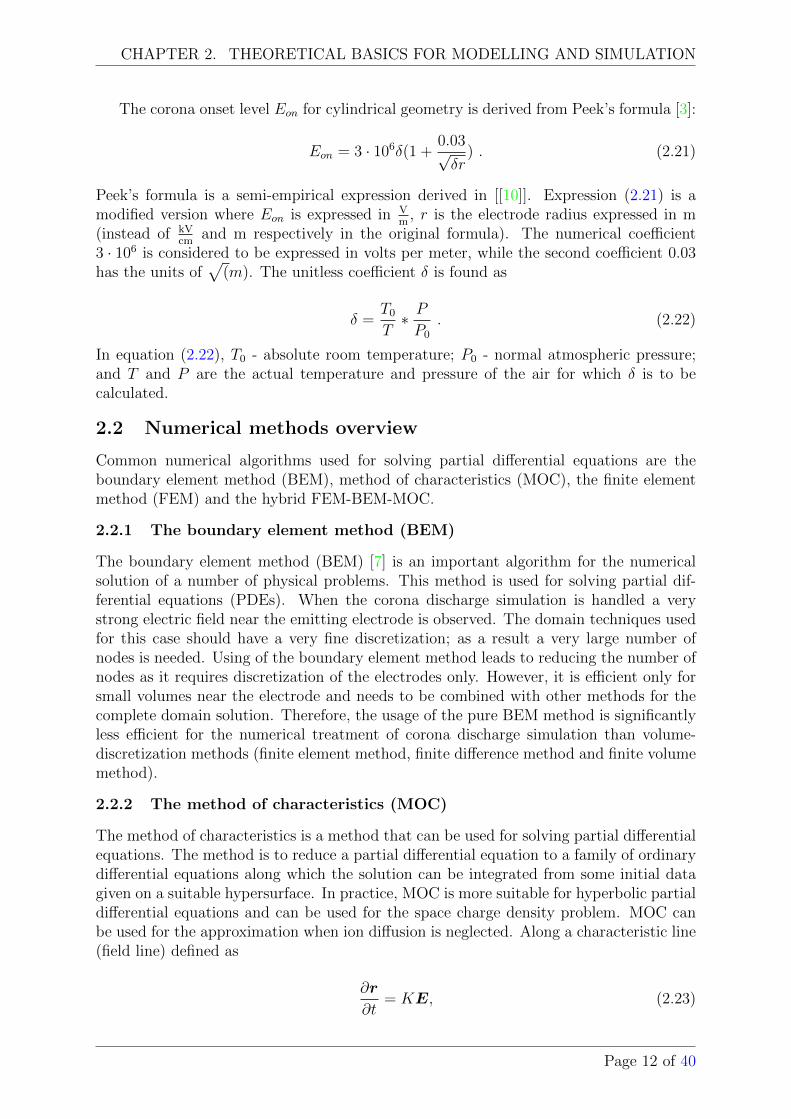
The corona onset level Eon for cylindrical geometry is derived from Peek’s formula [3]:

Eon = 3 · 106δ(1 +0.03√δr

) . (2.21)

Peek’s formula is a semi-empirical expression derived in [[10]]. Expression (2.21) is amodified version where Eon is expressed in V

m, r is the electrode radius expressed in m

(instead of kVcm

and m respectively in the original formula). The numerical coefficient3 · 106 is considered to be expressed in volts per meter, while the second coefficient 0.03has the units of

√(m). The unitless coefficient δ is found as

δ =T0

T∗ PP0

. (2.22)

In equation (2.22), T0 - absolute room temperature; P0 - normal atmospheric pressure;and T and P are the actual temperature and pressure of the air for which δ is to becalculated.

2.2 Numerical methods overview

Common numerical algorithms used for solving partial differential equations are theboundary element method (BEM), method of characteristics (MOC), the finite elementmethod (FEM) and the hybrid FEM-BEM-MOC.

2.2.1 The boundary element method (BEM)

The boundary element method (BEM) [7] is an important algorithm for the numericalsolution of a number of physical problems. This method is used for solving partial dif-ferential equations (PDEs). When the corona discharge simulation is handled a verystrong electric field near the emitting electrode is observed. The domain techniques usedfor this case should have a very fine discretization; as a result a very large number ofnodes is needed. Using of the boundary element method leads to reducing the number ofnodes as it requires discretization of the electrodes only. However, it is efficient only forsmall volumes near the electrode and needs to be combined with other methods for thecomplete domain solution. Therefore, the usage of the pure BEM method is significantlyless efficient for the numerical treatment of corona discharge simulation than volume-discretization methods (finite element method, finite difference method and finite volumemethod).

2.2.2 The method of characteristics (MOC)

The method of characteristics is a method that can be used for solving partial differentialequations. The method is to reduce a partial differential equation to a family of ordinarydifferential equations along which the solution can be integrated from some initial datagiven on a suitable hypersurface. In practice, MOC is more suitable for hyperbolic partialdifferential equations and can be used for the space charge density problem. MOC canbe used for the approximation when ion diffusion is neglected. Along a characteristic line(field line) defined as

∂r

∂t= KE, (2.23)

Page 12 of 40


the charge density satisfies an ordinary differential equation [18] which can also be derivedfrom (2.12 - 2.19)

∂ρ

∂t= −Kρ2/ε0 (2.24)

as a combination of the current density and the charge conservation law. The Equation(2.24) has a simple solution [7]

1

ρ=

1

ρ0

+Kt

ε0

. (2.25)

The characteristic lines are traced from those points on the corona electrode surface wherethe electric field is larger than the onset field, as only at those points the electric charge isinjected. The charge from the initial point with value ρ0 on the corona electrode decaysto the collecting electrode along the characteristic field line.

The methods described above (BEM and MOC) are given as a short overview andare not further used in this particular paper. All further computations and simulationsinvolve the finite element method.

2.2.3 The finite element method (FEM)

The Finite Element Method (FEM) is a powerful numerical method for solving partialdifferential and integral equations arising in physical problems. In the finite elementmethod the model is divided into separate parts - finite elements, connected to eachother in nodes. The connected finite elements create a mesh of the studied model. Theadvantage of the method is that the shape of the treated area can be arbitrary and themesh can be sparser in areas where special accuracy is not necessary. In the coronadischarge problem, a fine mesh is used close to the emitting electrode, because a largegradient of the electric field is required. At the same time, a large mesh can be used inareas where the variation of the voltage is relatively small, and also in areas which arenot of large interest for the particular calculation. Therefore, before the creation of thefinite element mesh it is necessary to allocate estimated areas of concentration of voltage.For the ESP geometry, these are the electrodes [19].

From a mathematical point of view the finite element method is a generalization ofthe Rayleigh-Ritz-Galerkin method. Therefore, it can be applied to a wide class of PDEs.After the studied area is divided into smaller pieces, which may be triangles or rectangles,a test function is given within each finite element in a simple way - usually, a polynomialof the third or fourth degree. Boundary conditions are much easier to put along the sidesof a triangle or rectangle than on the entire boundary. Each test function ϕ(x) is equalto zero in most of the region and is different from zero only in the neighbourhood of anode. The calculation accuracy is improved by a finer partition of the area [19].

A major problem is to investigate the accuracy of the solution obtained with theapproximation by a polynomial function. In other words, it is necessary to identify howwell the finite elements are constructed on the basis of computational simplicity, and ifthey would give a good approximation. It is intuitively clear that any sufficiently goodfunction can be approximated arbitrarily closely by linear functions. The mathematicalproblem is to obtain the best estimate of the error and determining the rate of decreaseof the error with increasing number of elements of the partition (or the degree of thepolynomial in each element).

Page 13 of 40


The basis of most CAD systems uses the finite element method. COMSOL Multi-physics software uses the finite element method for solving differential equations.

2.3 COMSOL Multiphysics

COMSOL Multiphysics is a very powerful system that allows to solve a wide class bound-ary value problems by means of the finite element method. Finite element analysis, whichis used in the program, is run together with an adaptive mesh (if selected) and an er-ror control using a variety of numerical solvers. COMSOL Multiphysics records all thesteps, such as parametric data, the model geometry, mesh, various solvers, visualizationand presentation of results during the simulation process. The structure of the programmakes it very easy to change any of the parameters of the model. It only requires chang-ing a corresponding node in the model tree and restart the sequence. The program storesand reapplies all other information and the data model. In COMSOL the user can in-dependently set the equations that describe a process, and the boundary conditions areset in familiar mathematical form using the Dirichlet and Neumann forms. COMSOLMultiphysics allows creating triangular, quadrilateral, tetrahedral and hexahedral com-putational grid. The mesh generator works quite well with a complex geometry and hasmany features to improve the grid. The post-processor has all the necessary features andoptions for visualization and processing of numerical data.

The efficiency and accuracy of FEM and COMSOL Multiphysics software for the ESPmodelling problems is proved in [20], [5], [14], [21] by comparing results of the simulationwith experimental data and therefore will be used for modelling and simulation in thiswork.

Page 14 of 40

Chapter 3

Modelling and simulation

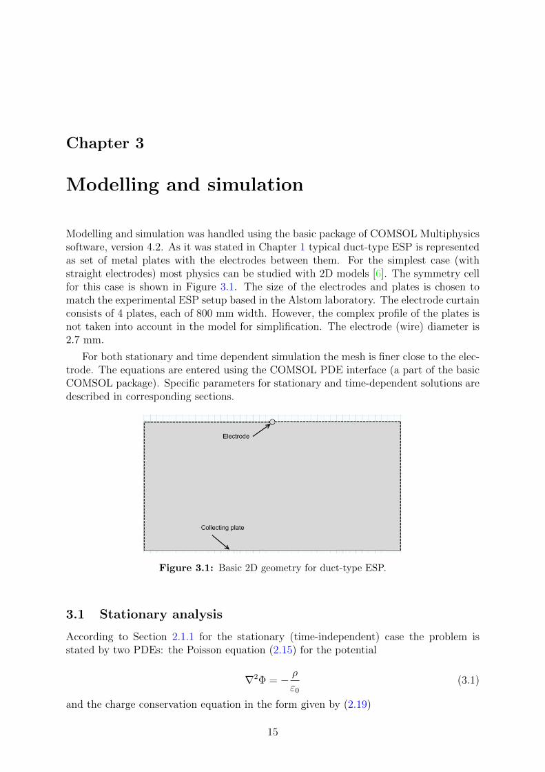
Modelling and simulation was handled using the basic package of COMSOL Multiphysicssoftware, version 4.2. As it was stated in Chapter 1 typical duct-type ESP is representedas set of metal plates with the electrodes between them. For the simplest case (withstraight electrodes) most physics can be studied with 2D models [6]. The symmetry cellfor this case is shown in Figure 3.1. The size of the electrodes and plates is chosen tomatch the experimental ESP setup based in the Alstom laboratory. The electrode curtainconsists of 4 plates, each of 800 mm width. However, the complex profile of the plates isnot taken into account in the model for simplification. The electrode (wire) diameter is2.7 mm.

For both stationary and time dependent simulation the mesh is finer close to the elec-trode. The equations are entered using the COMSOL PDE interface (a part of the basicCOMSOL package). Specific parameters for stationary and time-dependent solutions aredescribed in corresponding sections.

Figure 3.1: Basic 2D geometry for duct-type ESP.

3.1 Stationary analysis

According to Section 2.1.1 for the stationary (time-independent) case the problem isstated by two PDEs: the Poisson equation (2.15) for the potential

∇2Φ = − ρ

ε0

(3.1)

and the charge conservation equation in the form given by (2.19)

15

CHAPTER 3. MODELLING AND SIMULATION

∇Φ · ∇ρ− ρ2

ε0

= 0 (3.2)

For solving the PDEs within the specified geometry, boundary conditions are needed. Asimple Dirichlet boundary condition

Φ = 0, (3.3)

is used for the potential on the plates, and on the electrode

Φ = U, (3.4)

where U is the operating voltage of the ESP. However, the boundary conditions for thecharge density bring the main complexity to the problem. Two approaches for settingup the boundary conditions were chosen here giving the possibilities to study differentparameters. Both approaches are described in the following sections.

3.1.1 Direct implementation of Peek-Kaptzov model

The first approach uses Peek’s value for corona onset field strength Eon and Kaptzov’s as-sumption. Peek’s condition states that when the field strength exceeds the onset value thecharge density at the discharge electrode becomes non-zero [10]. The Kaptzov hypothesispostulates that with the increase of the potential difference between the electrodes theelectric field increases proportionally to the potential difference and only low discharge(dependent on residual ionization) with a very weak current takes place. When the onsetvoltage is reached the corona discharge starts and the field on the inner boundary of the“coronating” layer stays close to the corona onset value [11] The charge density at theboundary increases in such a way that the charge supplied to the domain balances theelectric field to stay at Eon.

The onset field value is set as a Neumann boundary condition on the electrode forthe Poisson’s equation (COMSOL node “Flux/Source” is used) giving the constant valueof electric field on the boundary. The onset field value is calculated for the geometrydescribed above using Peek’s formula for δ = 1 and equals Eon = 5.7 · 106 V

m.

For further steps the following reasoning is needed. If the current density from theelectrode value is given the current can be calculated by integration:

I =

∫S

J · dS =

∫S

Jn · dS. (3.5)

For convenience in the 2D model the current per meter of wire (electrode) Iw can be usedinstead. This can be achieved by integration over the electrode’s cross-section boundaryL:

Iw =

∫L

Jn · dL. (3.6)

The current density is

J = ρKE. (3.7)

By integration of (3.7) taking into account that ρ and En = Eon are constants on theboundary the following result is obtained

Iw = ρKEon

∫L

dL = ρKEon · 2πrw, (3.8)

Page 16 of 40


where rw is the electrode radius and the ideal cylindrical electrode is considered. Assum-ing that length (height) of the electrode is equal to the height of the plate, it is thenpossible to derive the current per square meter of the plate Ip by distributing Iw over theplate element with the horizontal (along the gas flow direction) length Lp, which for twosymmetric plates gives:

Ip =2πrwρKEon

2 · Lp. (3.9)

Now the boundary condition value for ρ can be derived from (3.9):

ρ =2 · Ip · Lp

2πrwKEon. (3.10)

Given the current Ip = 500µAm2 and considering the previous reasoning the BC value

for charge density on the electrode is ρ0 = 4.6 · 10−5 Cm3 . Note that the symmetry cell

used for further simulations includes only one plate and a half of the electrode.

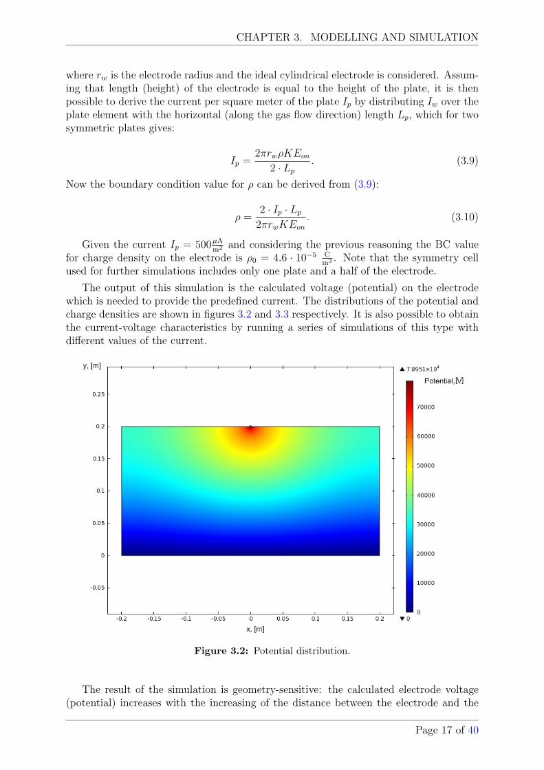
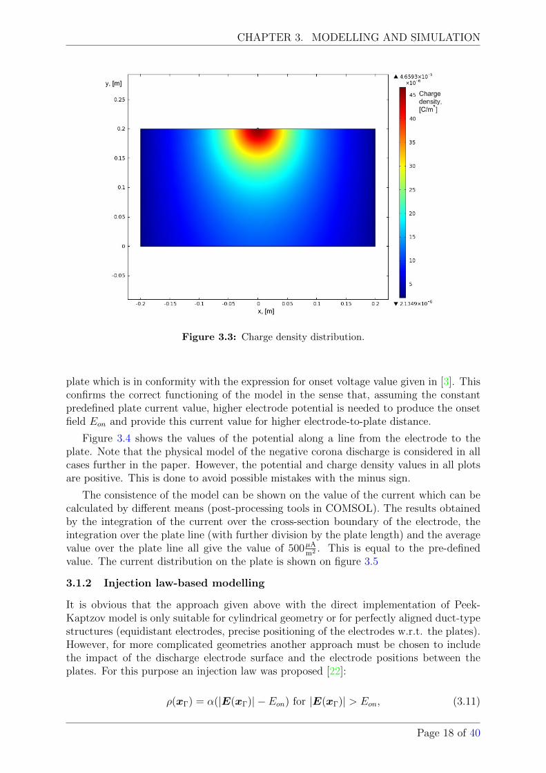
The output of this simulation is the calculated voltage (potential) on the electrodewhich is needed to provide the predefined current. The distributions of the potential andcharge densities are shown in figures 3.2 and 3.3 respectively. It is also possible to obtainthe current-voltage characteristics by running a series of simulations of this type withdifferent values of the current.

Figure 3.2: Potential distribution.

The result of the simulation is geometry-sensitive: the calculated electrode voltage(potential) increases with the increasing of the distance between the electrode and the

Page 17 of 40


Figure 3.3: Charge density distribution.

plate which is in conformity with the expression for onset voltage value given in [3]. Thisconfirms the correct functioning of the model in the sense that, assuming the constantpredefined plate current value, higher electrode potential is needed to produce the onsetfield Eon and provide this current value for higher electrode-to-plate distance.

Figure 3.4 shows the values of the potential along a line from the electrode to theplate. Note that the physical model of the negative corona discharge is considered in allcases further in the paper. However, the potential and charge density values in all plotsare positive. This is done to avoid possible mistakes with the minus sign.

The consistence of the model can be shown on the value of the current which can becalculated by different means (post-processing tools in COMSOL). The results obtainedby the integration of the current over the cross-section boundary of the electrode, theintegration over the plate line (with further division by the plate length) and the averagevalue over the plate line all give the value of 500µA

m2 . This is equal to the pre-definedvalue. The current distribution on the plate is shown on figure 3.5

3.1.2 Injection law-based modelling

It is obvious that the approach given above with the direct implementation of Peek-Kaptzov model is only suitable for cylindrical geometry or for perfectly aligned duct-typestructures (equidistant electrodes, precise positioning of the electrodes w.r.t. the plates).However, for more complicated geometries another approach must be chosen to includethe impact of the discharge electrode surface and the electrode positions between theplates. For this purpose an injection law was proposed [22]:

ρ(xΓ) = α(|E(xΓ)| − Eon) for |E(xΓ)| > Eon, (3.11)

Page 18 of 40


where x is the coordinate vector (x, y, z) (or (x, y) for the 2D case); Γ stands for theboundary of the electrode.

Figure 3.4: Potential along the wire-plate line.

Figure 3.5: Current profile on the collecting plate.

Page 19 of 40


If the value of α is large the exact functional relationship becomes insignificant andexpression (3.11) forms the Peek-Kaptzov condition. Being introduced to the system ofcoupled PDEs, it provides the dependence of the charge density on the local electric fieldat the discharge electrode surface. The main disadvantage of this formulation is thatwith a large α value the system becomes strongly non-linear, which leads to convergenceproblems. Studies of the convergence for different values of parameter α have been donein [5]. The value for α can be estimated by combining the current flow out from thestraight electrode

i = 2πrwK|E(xΓ)|ρ(xΓ) (3.12)

with the injection law (3.11). Let

δ =|E(xΓ)| − Eon|E(xΓ)|

(3.13)

be the relative error in the Kaptzov assumption for |E(xΓ)| > Eon. A combination of(3.12) - (3.13) yields that

α =i

2πrwK|E(xΓ)|2· 1

δ. (3.14)

Therefore, the value of the parameter α that leads to the Peek-Kaptzov treatmentshould be chosen such that

α >imax

2πrwKE2on

· 1

δfor |E(xΓ)| > Eon, (3.15)

where imax is the highest current to be handled (per meter of the discharge electrode) [5].

In order to run this type of simulation several changes must be done to the modeldescribed above. To improve the convergence for numerical solution the diffusion termshould be kept in the continuity equation as in (2.18)

K · (∇Φ · ∇ρ− ρ2

ε0

) +D∇2ρ = 0. (3.16)

The boundary condition for the charge density on the electrode is changed to theinjection law. Peek’s value for the onset field strength is no longer explicitly set as aboundary condition. It is now obtained by the correct choice of α for the injection law(3.11) (an example will follow below). The potential on the electrode is now set as anordinary Dirichlet BC according to (3.4).

Good convergence is achieved by using a 3-step calculation: solving separately thePoisson equation (3.1) (with ρ = 0); solving both PDEs (3.1) and (3.2) for ρ only (usingthe values of Φ obtained from the first step in each point); solving (3.1) and (3.2) forboth variables using the results of the previous two steps as initial values.

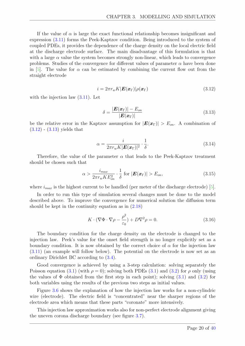
Figure 3.6 shows the explanation of how the injection law works for a non-cylindricwire (electrode). The electric field is “concentrated” near the sharper regions of theelectrode area which means that these parts “coronate” more intensively.

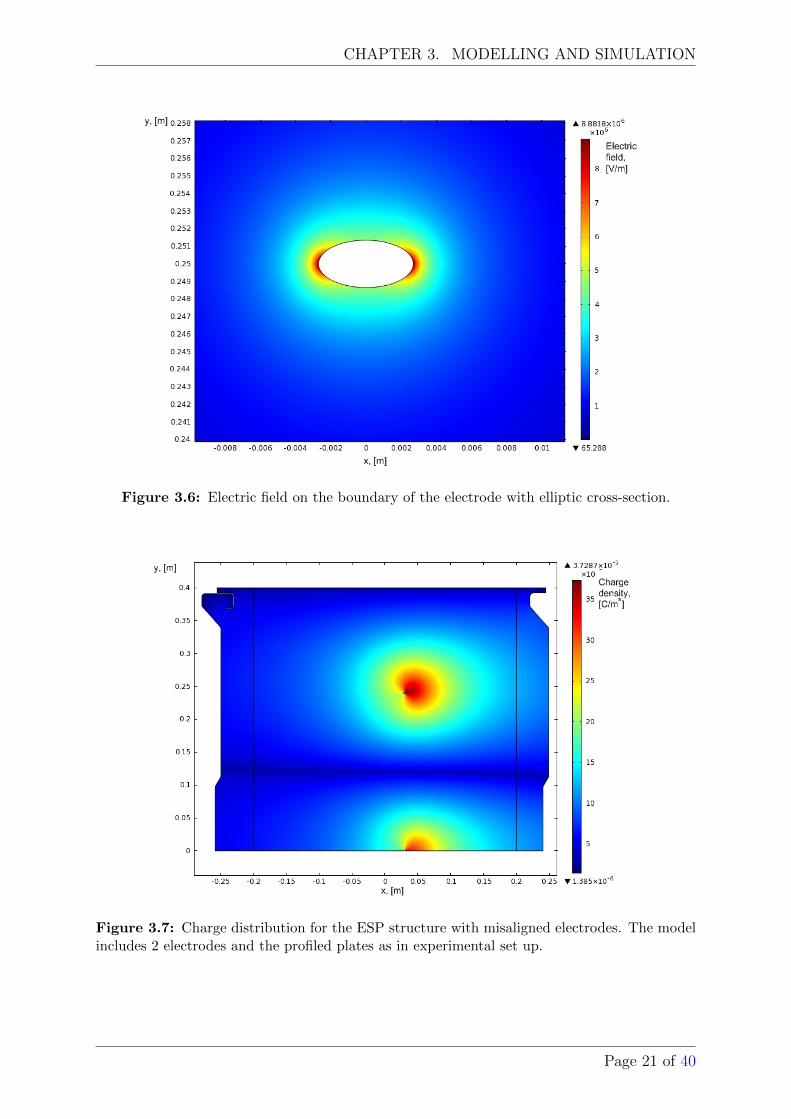
This injection law approximation works also for non-perfect electrode alignment givingthe uneven corona discharge boundary (see figure 3.7).

Page 20 of 40


Figure 3.6: Electric field on the boundary of the electrode with elliptic cross-section.

Figure 3.7: Charge distribution for the ESP structure with misaligned electrodes. The modelincludes 2 electrodes and the profiled plates as in experimental set up.

Page 21 of 40


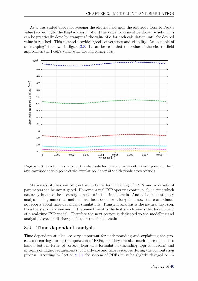
As it was stated above for keeping the electric field near the electrode close to Peek’svalue (according to the Kaptzov assumption) the value for α must be chosen wisely. Thiscan be practically done by “ramping” the value of α for each calculation until the desiredvalue is reached. This method provides good convergence and visibility. An example ofα “ramping” is shown in figure 3.8. It can be seen that the value of the electric fieldapproaches the Peek’s value with the increasing of α.

Figure 3.8: Electric field around the electrode for different values of α (each point on the xaxis corresponds to a point of the circular boundary of the electrode cross-section).

Stationary studies are of great importance for modelling of ESPs and a variety ofparameters can be investigated. However, a real ESP operates continuously in time whichnaturally leads to the necessity of studies in the time domain. And although stationaryanalyses using numerical methods has been done for a long time now, there are almostno reports about time-dependent simulations. Transient analysis is the natural next stepfrom the stationary one and in the same time it is the first step towards the developmentof a real-time ESP model. Therefore the next section is dedicated to the modelling andanalysis of corona discharge effects in the time domain.

3.2 Time-dependent analysis

Time-dependent studies are very important for understanding and explaining the pro-cesses occurring during the operation of ESPs, but they are also much more difficult tohandle both in terms of correct theoretical formulation (including approximations) andin terms of higher requirements for hardware and time resources during the computationprocess. Acording to Section 2.1.1 the system of PDEs must be slightly changed to in-

Page 22 of 40


clude time dependency. This concerns adding the time derivative of charge density intothe continuity equation (3.16) (see (2.12) and (2.16)) and setting up a time-dependentboundary condition on the electrode for one of the variables.

3.2.1 Current-controlled model

Power sources used for energizing the industrial ESPs physically represent the currentsources. Therefore it is more natural to use current pulses then voltage pulses duringthe simulation. Industrial ESP is usually fed by current pulses with the duration in therange of milliseconds. The motivation for the pulsating power supply is described in manypapers on ESPs and corona discharge, including [3] and [11]. In particular, [11] statesthat when the field structure in the outer domain of the discharge volume is distortedby space charges, less voltage falls on the coronating layer. Therefore the ionization ratedecreases. The discharge process becomes stationary with comparably small current. Thevoltage which drops on the discharge layer would not be enough for keeping the high rateof the current. This explains why a pulsating current is used in the ESP for producingcorona discharges with high values of the current.

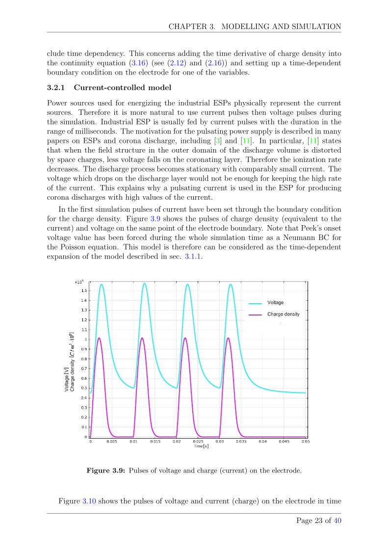
In the first simulation pulses of current have been set through the boundary conditionfor the charge density. Figure 3.9 shows the pulses of charge density (equivalent to thecurrent) and voltage on the same point of the electrode boundary. Note that Peek’s onsetvoltage value has been forced during the whole simulation time as a Neumann BC forthe Poisson equation. This model is therefore can be considered as the time-dependentexpansion of the model described in sec. 3.1.1.

Figure 3.9: Pulses of voltage and charge (current) on the electrode.

Figure 3.10 shows the pulses of voltage and current (charge) on the electrode in time

Page 23 of 40


domain. From the delays in the current values calculated on the electrode and on theplate it can be concluded that the charge density spreads as a wave in the domain (seefigure 3.10). A good visual representation of this wave can be obtained by making ananimated plot of the charge density over a line from the electrode to the plate, which canbe done by means of COMSOL tools. Unfortunately, there is no possibility to includesuch a plot into the paper, and a series of frame-by-frame plots would not be valuable inthis case.

Figure 3.10: Current and voltage change in time.

Figure 3.11 shows the voltage shape on the electrode when the system is fed by thecurrent pulses. From physical reasoning and the figure it can be concluded that the ESPsystem can be approximately represented by a parallel RC circuit shown in figure 3.12.

Page 24 of 40


Figure 3.11: Current (charge) and voltage pulses.

Page 25 of 40


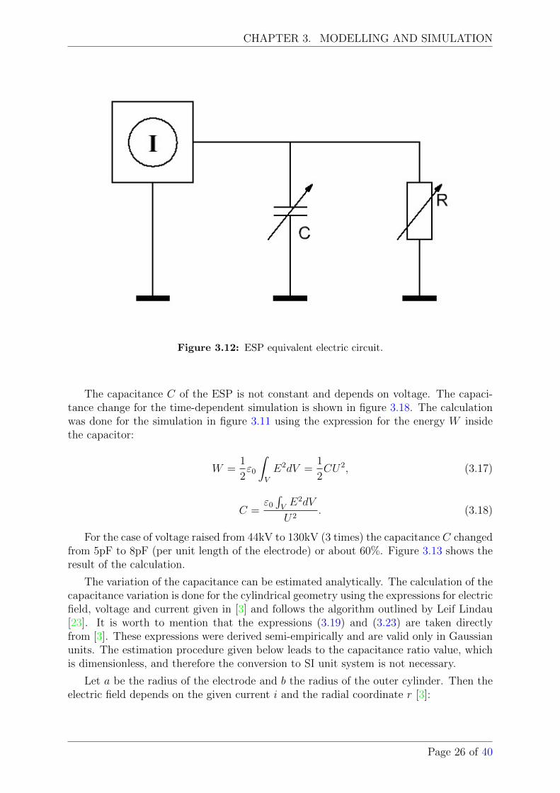
Figure 3.12: ESP equivalent electric circuit.

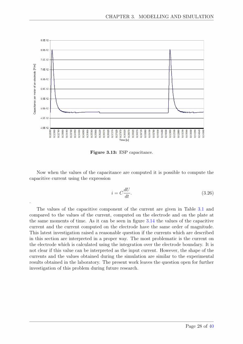
The capacitance C of the ESP is not constant and depends on voltage. The capaci-tance change for the time-dependent simulation is shown in figure 3.18. The calculationwas done for the simulation in figure 3.11 using the expression for the energy W insidethe capacitor:

W =1

2ε0

∫V

E2dV =1

2CU2, (3.17)

C =ε0

∫VE2dV

U2. (3.18)

For the case of voltage raised from 44kV to 130kV (3 times) the capacitance C changedfrom 5pF to 8pF (per unit length of the electrode) or about 60%. Figure 3.13 shows theresult of the calculation.

The variation of the capacitance can be estimated analytically. The calculation of thecapacitance variation is done for the cylindrical geometry using the expressions for electricfield, voltage and current given in [3] and follows the algorithm outlined by Leif Lindau[23]. It is worth to mention that the expressions (3.19) and (3.23) are taken directlyfrom [3]. These expressions were derived semi-empirically and are valid only in Gaussianunits. The estimation procedure given below leads to the capacitance ratio value, whichis dimensionless, and therefore the conversion to SI unit system is not necessary.

Let a be the radius of the electrode and b the radius of the outer cylinder. Then theelectric field depends on the given current i and the radial coordinate r [3]:

Page 26 of 40


E(r) =

√2i

K+

(Eonr0

r

)2

, (3.19)

where r0 is the radius of corona region which can be approximately taken as r0 = a.Expression (3.18) for cylindrical geometry and 2D calculation becomes

C =2πε

∫ barE2(r)dr

U2. (3.20)

Taking into account (3.19) the integration gives

∫ b

a

r

(2i

K+

(aEonr

)2)dr =

i

K(b2 − a2) + (Eona)2ln

b

a. (3.21)

The onset field value can be expressed in terms of the onset voltage U0 as

Eon =U0

aln ba

, (3.22)

see [3]

According to [3] the current is given by

i = U(U − U0)2K

b2ln ba

. (3.23)

Combining (3.23), (3.22), (3.21) and (3.18) and taking into account that b� a gives

C =2πε

ln ba

· 2U2 − 2UU0 + U20

U2(3.24)

or

C

C0

=

(U0

U

)2

− 2U0

U+ 2. (3.25)

For U0 = 44kV and U = 130kV (3.25) gives CC0

= 1.44.

The analytical result of 44% variation in capacitance is close to simulation results,which confirms accuracy of the model. The possibility of describing the ESP by means ofa simple equivalent circuit can be used for monitoring and designing a real-time controllerfor the ESP system.

Page 27 of 40


Figure 3.13: ESP capacitance.

Now when the values of the capacitance are computed it is possible to compute thecapacitive current using the expression

i = CdU

dt. (3.26)

.

The values of the capacitive component of the current are given in Table 3.1 andcompared to the values of the current, computed on the electrode and on the plate atthe same moments of time. As it can be seen in figure 3.14 the values of the capacitivecurrent and the current computed on the electrode have the same order of magnitude.This latest investigation raised a reasonable question if the currents which are describedin this section are interpreted in a proper way. The most problematic is the current onthe electrode which is calculated using the integration over the electrode boundary. It isnot clear if this value can be interpreted as the input current. However, the shape of thecurrents and the values obtained during the simulation are similar to the experimentalresults obtained in the laboratory. The present work leaves the question open for furtherinvestigation of this problem during future research.

Page 28 of 40


Table 3.1: Results of the capacitive current calculation.

Time, s Capacitance,F/m

VoltagederivativedU/dt, V/s

Capacitivecurrent permeter ofwire, A/m

Current onthe elec-trode permeter ofwire, A/m

Current onthe plateper squaremeter ofplate, A/m2

0,1201 4,78 ·10−12 7,52·107 3,60·10−4 3,85·10−4 1,89·10−12

0,1202 5,02·10−12 7,52·107 3,78·10−4 1,20·10−3 2,96·10−12

0,1203 5,40·10−12 7,52·107 4,06·10−4 1,20·10−3 3,99·10−12

0,1204 5,79·10−12 7,52·107 4,36·10−4 1,20·10−3 4,83·10−12

0,1206 6,18·10−12 7,52·107 4,64·10−4 1,20·10−3 5,37·10−12

0,1207 6,53·10−12 7,52·107 4,91·10−4 1,20·10−3 5,23·10−12

0,1208 6,87·10−12 7,52·107 5,16·10−4 1,20·10−3 1,10·10−9

0,1209 7,17·10−12 7,52·107 5,39·10−4 1,20·10−3 1,22·10−7

0,1211 7,59·10−12 -4,18·107 -3,17·10−4 0 1,31·10−6

0,1212 7,86·10−12 -3,98·107 -3,13·10−4 0 1,28·10−5

0,1213 7,98·10−12 -3,78·107 -3,02·10−4 0 7,93·10−5

0,1214 8,03·10−12 -3,60·107 -2,89·10−4 0 2,29·10−4

0,1216 8,01·10−12 -3,42·107 -2,74·10−4 0 4,67·10−4

Figure 3.14: Current comparison.

Page 29 of 40


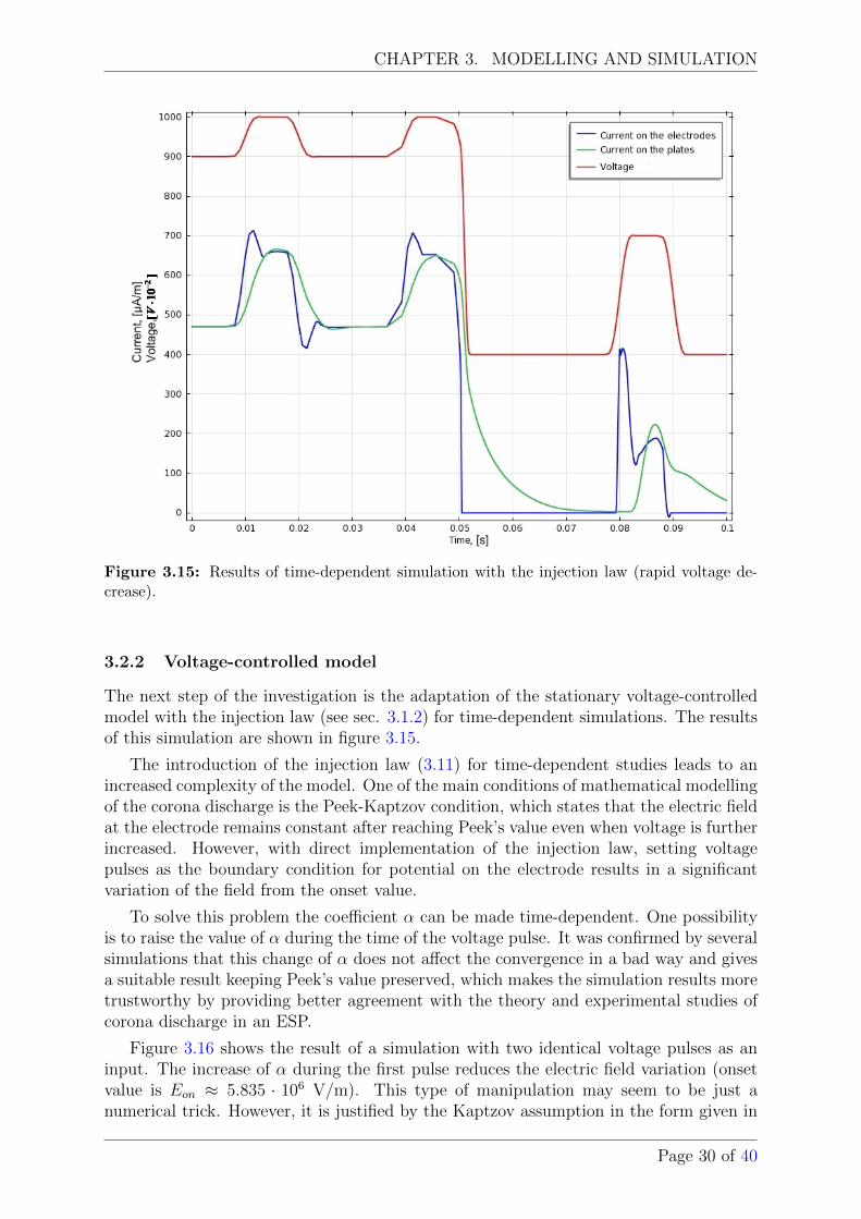
Figure 3.15: Results of time-dependent simulation with the injection law (rapid voltage de-crease).

3.2.2 Voltage-controlled model

The next step of the investigation is the adaptation of the stationary voltage-controlledmodel with the injection law (see sec. 3.1.2) for time-dependent simulations. The resultsof this simulation are shown in figure 3.15.

The introduction of the injection law (3.11) for time-dependent studies leads to anincreased complexity of the model. One of the main conditions of mathematical modellingof the corona discharge is the Peek-Kaptzov condition, which states that the electric fieldat the electrode remains constant after reaching Peek’s value even when voltage is furtherincreased. However, with direct implementation of the injection law, setting voltagepulses as the boundary condition for potential on the electrode results in a significantvariation of the field from the onset value.

To solve this problem the coefficient α can be made time-dependent. One possibilityis to raise the value of α during the time of the voltage pulse. It was confirmed by severalsimulations that this change of α does not affect the convergence in a bad way and givesa suitable result keeping Peek’s value preserved, which makes the simulation results moretrustworthy by providing better agreement with the theory and experimental studies ofcorona discharge in an ESP.

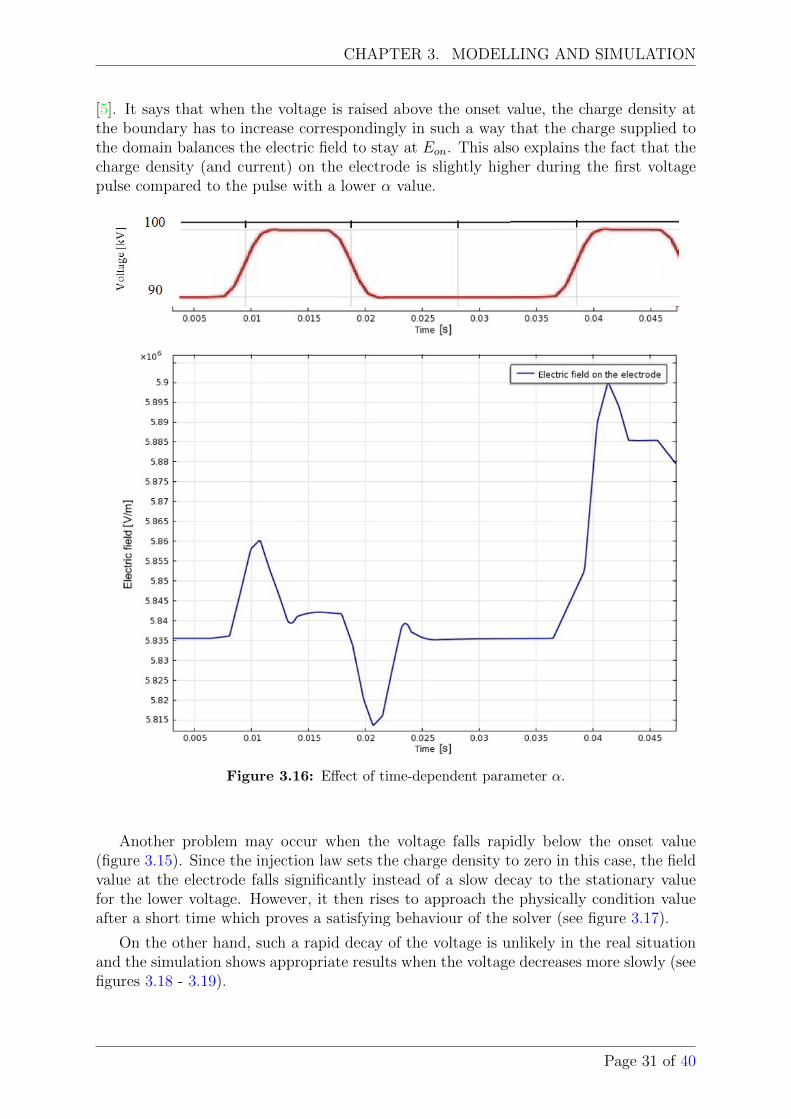
Figure 3.16 shows the result of a simulation with two identical voltage pulses as aninput. The increase of α during the first pulse reduces the electric field variation (onsetvalue is Eon ≈ 5.835 · 106 V/m). This type of manipulation may seem to be just anumerical trick. However, it is justified by the Kaptzov assumption in the form given in

Page 30 of 40


[5]. It says that when the voltage is raised above the onset value, the charge density atthe boundary has to increase correspondingly in such a way that the charge supplied tothe domain balances the electric field to stay at Eon. This also explains the fact that thecharge density (and current) on the electrode is slightly higher during the first voltagepulse compared to the pulse with a lower α value.

Figure 3.16: Effect of time-dependent parameter α.

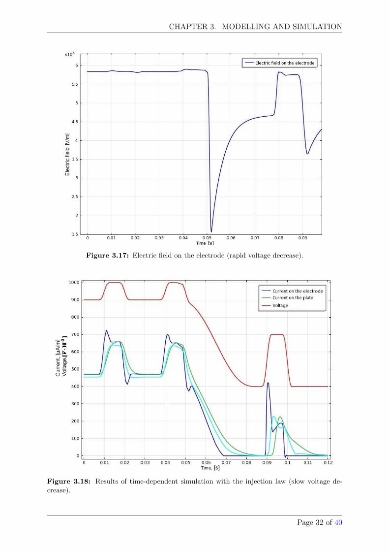
Another problem may occur when the voltage falls rapidly below the onset value(figure 3.15). Since the injection law sets the charge density to zero in this case, the fieldvalue at the electrode falls significantly instead of a slow decay to the stationary valuefor the lower voltage. However, it then rises to approach the physically condition valueafter a short time which proves a satisfying behaviour of the solver (see figure 3.17).

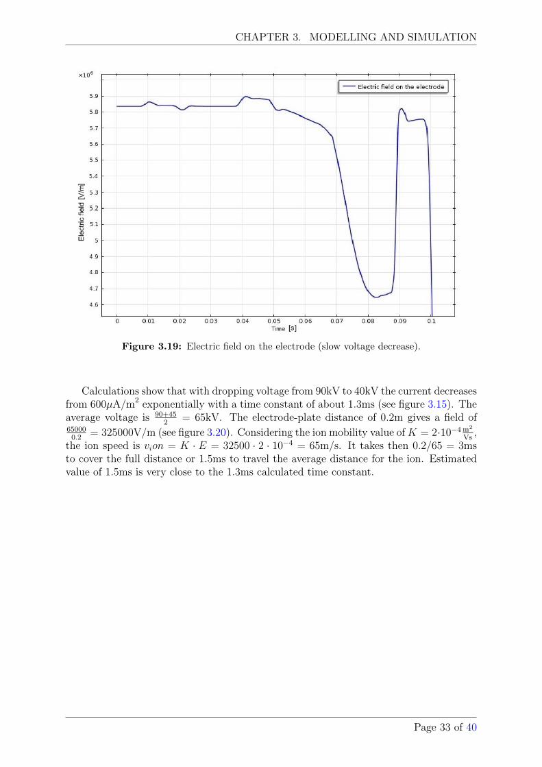
On the other hand, such a rapid decay of the voltage is unlikely in the real situationand the simulation shows appropriate results when the voltage decreases more slowly (seefigures 3.18 - 3.19).

Page 31 of 40


Figure 3.17: Electric field on the electrode (rapid voltage decrease).

Figure 3.18: Results of time-dependent simulation with the injection law (slow voltage de-crease).

Page 32 of 40


Figure 3.19: Electric field on the electrode (slow voltage decrease).

Calculations show that with dropping voltage from 90kV to 40kV the current decreasesfrom 600µA/m2 exponentially with a time constant of about 1.3ms (see figure 3.15). Theaverage voltage is 90+45

2= 65kV. The electrode-plate distance of 0.2m gives a field of

650000.2

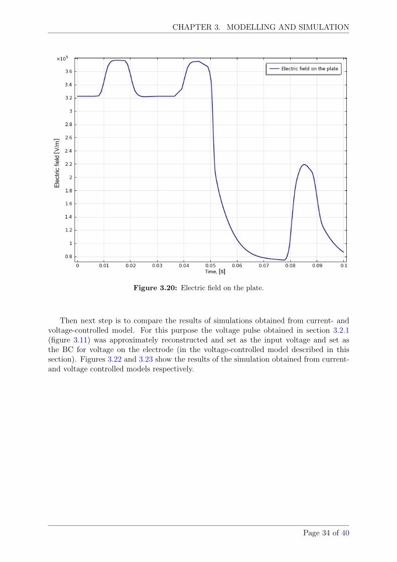
= 325000V/m (see figure 3.20). Considering the ion mobility value ofK = 2·10−4 m2

Vs,

the ion speed is vion = K · E = 32500 · 2 · 10−4 = 65m/s. It takes then 0.2/65 = 3msto cover the full distance or 1.5ms to travel the average distance for the ion. Estimatedvalue of 1.5ms is very close to the 1.3ms calculated time constant.

Page 33 of 40


Figure 3.20: Electric field on the plate.

Then next step is to compare the results of simulations obtained from current- andvoltage-controlled model. For this purpose the voltage pulse obtained in section 3.2.1(figure 3.11) was approximately reconstructed and set as the input voltage and set asthe BC for voltage on the electrode (in the voltage-controlled model described in thissection). Figures 3.22 and 3.23 show the results of the simulation obtained from current-and voltage controlled models respectively.

Page 34 of 40


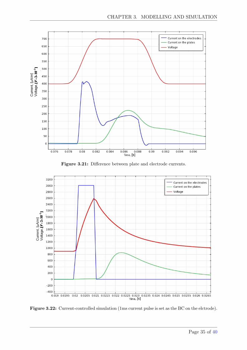
Figure 3.21: Difference between plate and electrode currents.

Figure 3.22: Current-controlled simulation (1ms current pulse is set as the BC on the elctrode).

Page 35 of 40


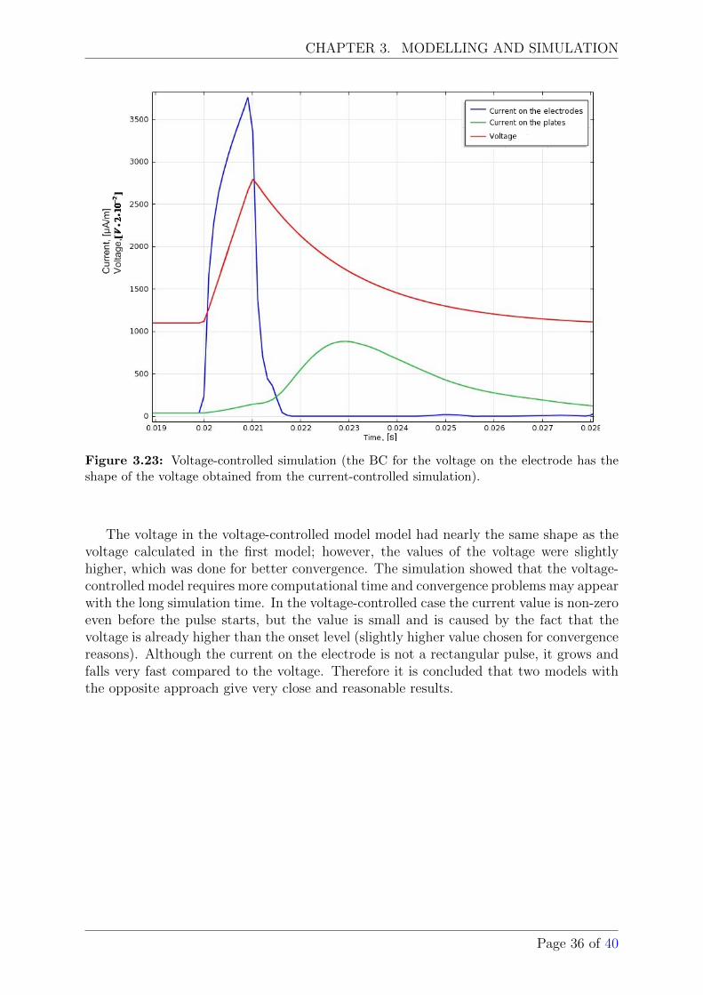
Figure 3.23: Voltage-controlled simulation (the BC for the voltage on the electrode has theshape of the voltage obtained from the current-controlled simulation).

The voltage in the voltage-controlled model model had nearly the same shape as thevoltage calculated in the first model; however, the values of the voltage were slightlyhigher, which was done for better convergence. The simulation showed that the voltage-controlled model requires more computational time and convergence problems may appearwith the long simulation time. In the voltage-controlled case the current value is non-zeroeven before the pulse starts, but the value is small and is caused by the fact that thevoltage is already higher than the onset level (slightly higher value chosen for convergencereasons). Although the current on the electrode is not a rectangular pulse, it grows andfalls very fast compared to the voltage. Therefore it is concluded that two models withthe opposite approach give very close and reasonable results.

Page 36 of 40

Chapter 4

Conclusions and discussion

The experiments described in the paper show the transition from stationary to time-dependent analysis. The models for stationary analysis, previously described in [5], [6], [7]etc. and approved by the ESP scientific society, were successfully recreated and simulatedby means of COMSOL Multiphysics software. Two models for stationary analysis withdifferent approach were proposed (see sec. 3.1), both showing good agreement with thetheory and experimental studies as expected.

Time-dependent simulations is a logical and very important step in ESP studies. Itallows to expand the knowledge of ESP systems and test their performance under certainconditions, previously impossible by means of stationary studies.

Two possible models for time-dependent simulation of corona discharge in an ESP, thecurrent-controlled and voltage-controlled model, were proposed in sections 3.2.1 and 3.2.2respectively. Both models are in good agreement with current theoretical investigationsand experimental analysis of ESP systems. However, the simulations with both modelsleave open questions about some of the results, see comments found in correspondingsections.

As to the difference in performance of two models, the computations are much fasterand there is no convergence problems with the current-controlled model. It is also moreconvenient because the power supplies for real ESPs are current sources. On the otherhand, the results obtained using this model can be misinterpreted (see sec. 3.2.1) andfurther research and laboratory experiments are needed for a complete approval of themodel. The voltage-controlled model is more difficult to handle in terms of computationtime and convergence, but it is more flexible and allows the study of the geometry featuresby using the injection law (3.11) for the charge density on the electrode.

It was shown that time-dependent simulations can be performed by means of modernsimulation software on an ordinary PC with reasonable computation times.

It is obvious, however, that the presented models are far from real-time models andfurther research and experiments on the matter are necessary.

The instructions for adaptation of the COMSOL Multiphysics software to the simula-tion of corona discharge in ESPs, inluding the time-dependent simulation, were developedfor internal use in ALSTOM AB.

37

Bibliography

[1] K. Porle, S.L. Francis, K.M. Bradburn, Electrostatic Precipitators for Industrial Ap-plications, Finland: Rehva, 2007.

[2] D. DalSanto. (2011, February 1). The Encyclopedia Of Filters - Dust Collection Sys-tems [Online]. Available:

http://www.baghouse.com/2011/02/01/

the-encyclopedia-of-filters-dust-collection-systems/

[3] H.J. White,Industrial electrostatic precipitation, Reading, MA: Addison-Wesley PubCo., 1963.

[4] B. Bellagamba et al. ”‘A Mathematical Model for Simulation of Large-Scale Electro-static Precipitators”’ in The International Conference on Electrostatic Precipitation(ICESP), Washington, DC USA, 1993.

[5] A. Back, J. Cramsky,”’Comparison of Numerical and Experimental Results for theDuct-Type Electrostatic Precipitator”’, International Journal of Plasma Environmen-tal Science & Technology, vol. 6, No 1, pp. 33-42, 2012.

[6] J. Cramsky, ”‘Computations for electrostatic precipitators using the finite elementmethod”’, M.S. Thesis, Eng. Physics Program, Univ. Lund LTH, Lund, Sweden,2010.

[7] P. Atten, K. Adamiak,”’Simulation of corona discharge in point-plane configuration”’,J. of Electrostatics, vol. 61, pp. 85-98, 2004.

[8] J. Townsend, Electricity in gases, Oxford: Clarendon Press, 1915.

[9] L. Loeb, Electrical Coronas, their basic physical mechanisms, Berkeley: University ofCalifornia Press, 1965.

[10] F.W. Peek Jr.,Dielectric phenomena in high voltage engineering. 3rd ed. New York,NY:McGraw-Hill, 1929.

[11] N.A. Kaptzov,Electrical phenomena in gases and vacuum (in Russian), Moscow:Ogiz, 1947.

[12] E. Warburg, ”‘Ueber die Spitzenentladung”’, Wiedemanns Annalen der Physik und.Chemie, vol. 67, pp. 69-83, 1899.

38

BIBLIOGRAPHY

[13] J.E. Almy, ”‘Discharge current from a surface of large curvature”’, Am. J. Sci., vol.12, pp. 175-179, 1901.

[14] B. Benamar, E. Favre, A. Donnot, M.O. Rigo, ”‘Finite Element Solution for Ion-ized Fields in DC Electrostatic Precipitator”’, COMSOL Users Conference, Grenoble,France, 2007.

[15] J. D. Jackson, Classical Electrodynamics, 3rd ed., New York: Wiley, 1999.

[16] L. Zhao, K. Adamiak, ”‘EHD Flow Produced by Electric Corona Discharge (Numer-ical and Experimental Studies, and Applications)”’, J. of Electrostatics, vol. 63, pp.337-350, 2005.

[17] J.O. Hirschfelder, C.F. Curtiss, R.B. Bird, Molecular Theory of Gases and Liquids,New York: Wiley,, 1954.

[18] K. Adamiak, ”‘Application of integral equations to solving inverse problems of sta-tionary electromagnetic fields”’, Int. J. Numer. Meth. Eng., vol. 21, pp. 14471458,1985.

[19] J.N. Reddy, An Introduction to the Finite Element Method, 3rd ed., McGraw-HillHigher Education, 2005.

[20] A. Muhammad, J. Muhammad,”’Modeling and Simulation of an Electrostatic Pre-cipitator”’, Degree project, School of Computer Sc., Pysics and Math., LinnaeusUniversity, Vaxjo, Sweden, 2011.

[21] Herek L. Clack, ”‘Computational Modeling of Electrohydrodynamically-InfluencedMercury Adsorption within ESPs”’ in International Conference on Electrostatic Pre-cipitation, Bangalore, India, 2013.

[22] P. Atten, K. Adamiak, B. Khaddour, J.-L. Coulomb,”’Simulation of corona dischargein configurations with a sharp electrode”’, Journal of Optoelectronics and AdvancedMaterials, vol. 6, pp. 1023-1028, 2004.

[23] L. Lindau, Private communication.

Page 39 of 40

Faculty of Technology SE-391 82 Kalmar | SE-351 95 Växjö Phone +46 (0)772-28 80 00 [email protected] Lnu.se/faculty-of-technology?l=en

time dependent modelling and simulation of the …707884/fulltext01.pdf · degree project time...

Documents