three lectures on dmrg in quantum chemistry - eth z lectures on dmrg in quantum chemistry ... from...
TRANSCRIPT
Three Lectures on DMRG in Quantum Chemistry
Markus Reiher
Laboratorium fur Physikalische Chemie, ETH Zurich, Switzerland
http://www.reiher.ethz.ch
February 2014
Version: 1.2 — 17/02/2014
DMRG in Quantum Chemistry Markus Reiher 1 / 96
Three Lectures on DMRG in Quantum Chemistry
1 First-Generation Density Matrix Renormalization Group (DMRG)
in Quantum Chemistry
2 Second-Generation DMRG:
Matrix Product and Tensor Network States
3 Some Results of Actual Quantum-Chemical Calculations
Very useful introductory reference:
U. Schollwock, The density-matrix renormalization group in the age of
matrix product states, arXiv: 1008.3477v2
DMRG in Quantum Chemistry Markus Reiher 2 / 96
Reviews on about 15 years of DMRG in Quantum
Chemistry ... for Further References
1 O Legeza, R. M. Noack, J. Solyom and L. Tincani, Applications of Quantum Information in the Density-Matrix
Renormalization Group, Lect. Notes Phys., 739,653-664 (2008)
2 G. K.-L. Chan, J. J. Dorando, D. Ghosh, J. Hachmann, E. Neuscamman, H. Wang, T. Yanai, An Introduction to the
Density Matrix Renormalization Group Ansatz in Quantum Chemistry, Prog. Theor. Chem. and Phys., 18, 49 (2008)
3 D. Zgid and G. K.-L. Chan, The Density Matrix Renormalisation Group in Quantum Chemistry, Ann. Rep. Comp.
Chem., 5, 149, (2009)
4 K. H. Marti, M. Reiher, The Density Matrix Renormalization Group Algorithm in Quantum Chemistry, Z. Phys. Chem.,
224, 583-599 (2010)
5 G. K.-L. Chan and S. Sharma, The density matrix renormalization group in quantum chemistry, Ann. Rev. Phys. Chem.,
62, 465 (2011)
6 K. H. Marti, M. Reiher, New Electron Correlation Theories for Transition Metal Chemistry, Phys. Chem. Chem. Phys.,
13, 6750-6759 (2011)
7 Y. Kurashige, Multireference electron correlation methods with density matrix renormalisation group reference functions,
Mol. Phys. in press (2014)
DMRG in Quantum Chemistry Markus Reiher 3 / 96
Lecture 1
First-Generation DMRG in Quantum Chemistry
1 Standard Configuration Interaction in Explicit Second Quantization
2 Dimension Reduction by Decimation
3 Elements of the DMRG Algorithm
DMRG in Quantum Chemistry Markus Reiher 4 / 96
Non-Relativistic Many-Electron Hamiltonian
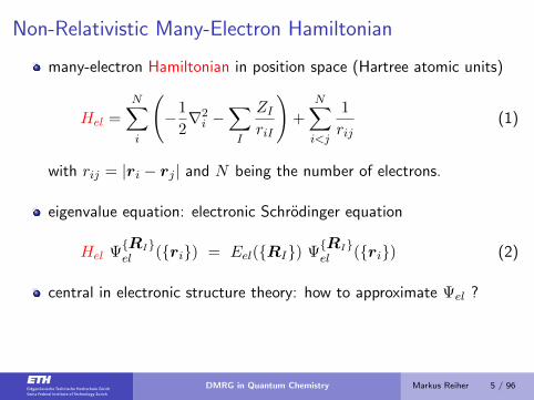
many-electron Hamiltonian in position space (Hartree atomic units)
Hel =
N∑i
(−1
2∇2i −
∑I
ZIriI
)+
N∑i<j
1
rij(1)
with rij = |ri − rj | and N being the number of electrons.
eigenvalue equation: electronic Schrodinger equation
Hel Ψ{RI}el ({ri}) = Eel({RI}) Ψ
{RI}el ({ri}) (2)
central in electronic structure theory: how to approximate Ψel ?
DMRG in Quantum Chemistry Markus Reiher 5 / 96
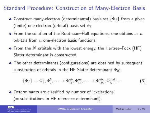
Standard Procedure: Construction of Many-Electron Basis
Construct many-electron (determinantal) basis set {ΦI} from a given
(finite) one-electron (orbital) basis set φi
From the solution of the Roothaan–Hall equations, one obtains as n
orbitals from n one-electron basis functions.
From the N orbitals with the lowest energy, the Hartree–Fock (HF)
Slater determinant is constructed.
The other determinants (configurations) are obtained by subsequent
substitution of orbitals in the HF Slater determinant Φ0:
{ΦI} → Φai ,Φ
bj , · · · → Φab
ij ,Φacik , · · · → Φabc
ijk ,Φabdijl , . . . (3)
Determinants are classified by number of ’excitations’
(= substitutions in HF reference determinant).
DMRG in Quantum Chemistry Markus Reiher 6 / 96
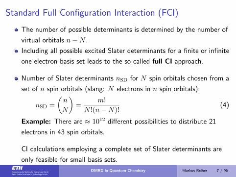
Standard Full Configuration Interaction (FCI)
The number of possible determinants is determined by the number of
virtual orbitals n−N .
Including all possible excited Slater determinants for a finite or infinite
one-electron basis set leads to the so-called full CI approach.
Number of Slater determinants nSD for N spin orbitals chosen from a
set of n spin orbitals (slang: N electrons in n spin orbitals):
nSD =
(n
N
)=
m!
N !(n−N)!(4)
Example: There are ≈ 1012 different possibilities to distribute 21
electrons in 43 spin orbitals.
CI calculations employing a complete set of Slater determinants are
only feasible for small basis sets.
DMRG in Quantum Chemistry Markus Reiher 7 / 96
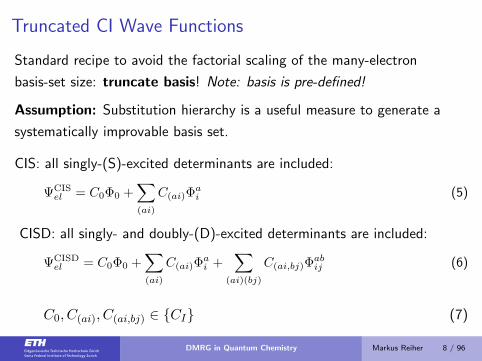
Truncated CI Wave Functions
Standard recipe to avoid the factorial scaling of the many-electron
basis-set size: truncate basis! Note: basis is pre-defined!
Assumption: Substitution hierarchy is a useful measure to generate a
systematically improvable basis set.
CIS: all singly-(S)-excited determinants are included:
ΨCISel = C0Φ0 +
∑(ai)
C(ai)Φai (5)
CISD: all singly- and doubly-(D)-excited determinants are included:
ΨCISDel = C0Φ0 +
∑(ai)
C(ai)Φai +
∑(ai)(bj)
C(ai,bj)Φabij (6)
C0, C(ai), C(ai,bj) ∈ {CI} (7)
DMRG in Quantum Chemistry Markus Reiher 8 / 96
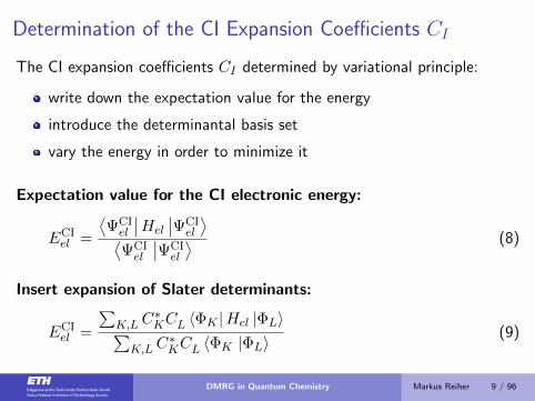
Determination of the CI Expansion Coefficients CI
The CI expansion coefficients CI determined by variational principle:
write down the expectation value for the energy
introduce the determinantal basis set
vary the energy in order to minimize it
Expectation value for the CI electronic energy:
ECIel =
⟨ΨCIel
∣∣Hel
∣∣ΨCIel
⟩⟨ΨCIel
∣∣ΨCIel
⟩ (8)
Insert expansion of Slater determinants:
ECIel =
∑K,LC
∗KCL 〈ΦK |Hel |ΦL〉∑
K,LC∗KCL 〈ΦK |ΦL〉
(9)
DMRG in Quantum Chemistry Markus Reiher 9 / 96
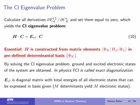
The CI Eigenvalue Problem
Calculate all derivatives ∂ECIel / ∂C
∗K and set them equal to zero, which
yields the CI eigenvalue problem:
H ·C = Eel ·C (10)
Essential: H is constructed from matrix elements 〈ΦK |Hel |ΦL〉 in
pre-defined determinantal basis {ΦK}
By solving the CI eigenvalue problem, ground and excited electronic states
of the system are obtained. In physics FCI is called exact diagonalization.
Eel is diagonal matrix with total energies of all electronic states that can
be expressed in basis given (M determinants yield M electronic states).
DMRG in Quantum Chemistry Markus Reiher 10 / 96
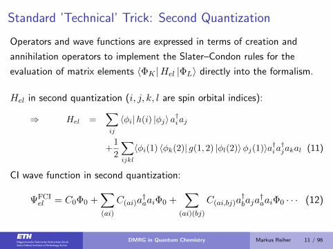
Standard ’Technical’ Trick: Second Quantization
Operators and wave functions are expressed in terms of creation and
annihilation operators to implement the Slater–Condon rules for the
evaluation of matrix elements 〈ΦK |Hel |ΦL〉 directly into the formalism.
Hel in second quantization (i, j, k, l are spin orbital indices):
⇒ Hel =∑ij
〈φi|h(i) |φj〉 a†iaj
+1
2
∑ijkl
〈φi(1) 〈φk(2)| g(1, 2) |φl(2)〉φj(1)〉a†ia†jakal (11)
CI wave function in second quantization:
ΨFCIel = C0Φ0 +
∑(ai)
C(ai)a†aaiΦ0 +
∑(ai)(bj)
C(ai,bj)a†baja
†aaiΦ0 · · · (12)
DMRG in Quantum Chemistry Markus Reiher 11 / 96
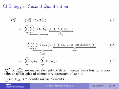
CI Energy in Second Quantization
ECIel =
⟨ΨCIel
∣∣∣Hel ∣∣∣ΨCIel
⟩(13)
=N∑ij
N∑KL
C∗KCLtKLij︸ ︷︷ ︸
γij
〈φi(1)|h(1) |φj(1)〉︸ ︷︷ ︸≡hij
+N∑ijkl
N∑KL
C∗KCLTKLijkl︸ ︷︷ ︸
Γijkl
〈φi(1) 〈φk(2)| g(1, 2) |φl(2)〉φj(1)〉︸ ︷︷ ︸gijkl
(14)
=N∑ij
γijhij +N∑ijkl
Γijklgijkl (15)
tKLij or TKLijkl are matrix elements of determinantal basis functions overpairs or quadruples of elementary operators a† and a.
γij are Γijkl are density matrix elements.
DMRG in Quantum Chemistry Markus Reiher 12 / 96
Is there a better way to construct the finite-dimensional
determinantal basis set in order to avoid the factorial scaling?
DMRG in Quantum Chemistry Markus Reiher 13 / 96
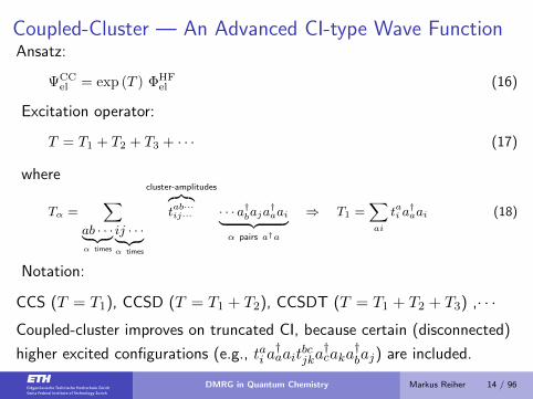
Coupled-Cluster — An Advanced CI-type Wave FunctionAnsatz:
ΨCCel = exp (T ) ΦHF
el (16)
Excitation operator:
T = T1 + T2 + T3 + · · · (17)
where
Tα =∑
ab · · ·︸ ︷︷ ︸α times
ij · · ·︸ ︷︷ ︸α times
cluster-amplitudes︷︸︸︷tab···ij··· · · · a†baja
†aai︸ ︷︷ ︸
α pairs a†a
⇒ T1 =∑ai
tai a†aai (18)
Notation:
CCS (T = T1), CCSD (T = T1 + T2), CCSDT (T = T1 + T2 + T3) ,· · ·
Coupled-cluster improves on truncated CI, because certain (disconnected)
higher excited configurations (e.g., tai a†aait
bcjka†caka
†baj) are included.
DMRG in Quantum Chemistry Markus Reiher 14 / 96
Is there a better way to construct the finite-dimensional
determinantal basis set in order to avoid the factorial scaling?
Let’s investigate FCI from a different perspective:
DMRG in Quantum Chemistry Markus Reiher 15 / 96
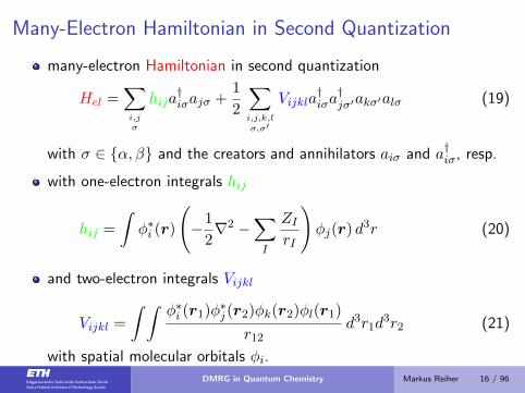
Many-Electron Hamiltonian in Second Quantization
many-electron Hamiltonian in second quantization
Hel =∑i,jσ
hija†iσajσ +
1
2
∑i,j,k,lσ,σ′
Vijkla†iσa†jσ′akσ′alσ (19)
with σ ∈ {α, β} and the creators and annihilators aiσ and a†iσ, resp.
with one-electron integrals hij
hij =
∫φ∗i (r)
(−1
2∇2 −
∑I
ZIrI
)φj(r) d3r (20)
and two-electron integrals Vijkl
Vijkl =
∫ ∫φ∗i (r1)φ∗j (r2)φk(r2)φl(r1)
r12d3r1d
3r2 (21)
with spatial molecular orbitals φi.
DMRG in Quantum Chemistry Markus Reiher 16 / 96
Full CI in (Explicit) Second Quantization
Elementary operators: a†iσ and aiσ
Hamiltonian matrix is now constructed from the matrix representation
for the elementary operators by direct products
By contrast to standard procedure, instead of evaluating the
action of the elementary operators on the determinantal basis
functions, we set-up a matrix representation of the elementary
operators and construct a matrix representation of the
Hamiltonian DIRECTLY.
This Hamiltonian matrix can then be diagonalized.
DMRG in Quantum Chemistry Markus Reiher 17 / 96
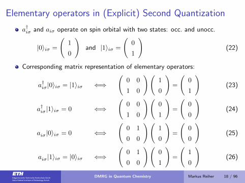
Elementary operators in (Explicit) Second Quantization
a†iσ and aiσ operate on spin orbital with two states: occ. and unocc.
|0〉iσ =
(1
0
)and |1〉iσ =
(0
1
)(22)
Corresponding matrix representation of elementary operators:
a†iσ|0〉iσ = |1〉iσ ⇐⇒
(0 0
1 0
)(1
0
)=
(0
1
)(23)
a†iσ|1〉iσ = 0 ⇐⇒
(0 0
1 0
)(0
1
)=
(0
0
)(24)
aiσ|0〉iσ = 0 ⇐⇒
(0 1
0 0
)(1
0
)=
(0
0
)(25)
aiσ|1〉iσ = |0〉iσ ⇐⇒
(0 1
0 0
)(0
1
)=
(1
0
)(26)
DMRG in Quantum Chemistry Markus Reiher 18 / 96
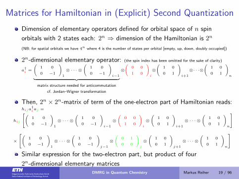
Matrices for Hamiltonian in (Explicit) Second Quantization
Dimension of elementary operators defined for orbital space of n spin
orbitals with 2 states each: 2n ⇒ dimension of the Hamiltonian is 2n
(NB: for spatial orbitals we have 4n where 4 is the number of states per orbital [empty, up, down, doubly occupied])
2n-dimensional elementary operator: (the spin index has been omitted for the sake of clarity)
a†i =
(1 0
0 −1
)1
⊗ · · · ⊗(
1 0
0 −1
)i−1︸ ︷︷ ︸
matrix structure needed for anticommutation
cf. Jordan–Wigner transformation
⊗(
0 0
1 0
)i
⊗(
1 0
0 1
)i+1
⊗· · ·⊗(
1 0
0 1
)n
Then, 2n × 2n-matrix of term of the one-electron part of Hamiltonian reads:hija
†iaj =
hij
( 1 0
0 −1
)1
⊗ · · · ⊗(
1 0
0 −1
)i−1
⊗(
0 0
1 0
)i
⊗(
1 0
0 1
)i+1
⊗ · · · ⊗(
1 0
0 1
)n
×
( 1 0
0 −1
)1
⊗ · · · ⊗(
1 0
0 −1
)j−1
⊗(
0 1
0 0
)j
⊗(
1 0
0 1
)j+1
⊗ · · · ⊗(
1 0
0 1
)n
Similar expression for the two-electron part, but product of four
2n-dimensional elementary matricesDMRG in Quantum Chemistry Markus Reiher 19 / 96
Nothing has been gained yet!
Even worse: Huge matrices have been generated which contain
mostly zeros and need to be multiplied and added.
DMRG in Quantum Chemistry Markus Reiher 20 / 96
Nothing has been gained yet!
Even worse: Huge matrices have been generated which contain
mostly zeros and need to be multiplied and added.
Need to find a way to reduce the dimension !
DMRG in Quantum Chemistry Markus Reiher 21 / 96
What is the best reduced many-particle basis?
First attempt: Wilson’s renormalization group
DMRG in Quantum Chemistry Markus Reiher 22 / 96
Wilson’s Renormalization Group: Dimension Reduction
1 Choose a number of orbitals l whose many-electron Hamiltonian H(l)el
can still be constructed and exactly diagonalized.
2 Diagonalize H(l)el of dimension 2l (or 4l for spatial orbitals) and select
m lowest-energy eigenvectors out of the 2l eigenvectors.
3 Reduce the dimension of H(l)el from 2l to m by transformation with
the rectangular m× 2l matrix of eigenvectors.
4 Construct H(l+1)el from H
(l)el and H
(1)el defined for an orbital taken
from the L− l remaining orbitals.
5 Continue with 2) until l + 1 = L.
DMRG in Quantum Chemistry Markus Reiher 23 / 96
Issues with Wilson’s Renormalization Group
H(l)el requires exact diagonalization (or a subspace iteration technique
like Lanczos, which produces a large portion of the low-energy
eigenvectors) and thus its dimension 2l is limited and l must therefore
be rather small
No guarantee that the reduced basis is an optimum choice in some
sense.
No information from those L− l remaining orbitals, which have not
yet been considered, are taken into account in the construction of
H(l)el (particularly bad, when l is small)
DMRG in Quantum Chemistry Markus Reiher 24 / 96
What is the best reduced many-particle basis in terms of a
least-squares fit?
Second attempt: White’s DMRG
— transform with eigenvectors of a reduced density matrix
S. R. White, Phys. Rev. Lett. 1992 69 2863; Phys. Rev. B 1993 48 10345
DMRG in Quantum Chemistry Markus Reiher 25 / 96
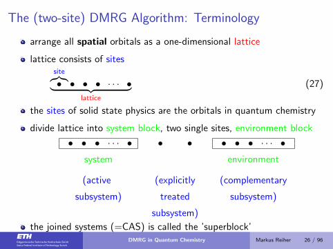
The (two-site) DMRG Algorithm: Terminology
arrange all spatial orbitals as a one-dimensional lattice
lattice consists of sitessite︷︸︸︷• • • • · · · •︸ ︷︷ ︸
lattice
(27)
the sites of solid state physics are the orbitals in quantum chemistry
divide lattice into system block, two single sites, environment block
• • • · · · • • • • • • · · · •system environment
(active (explicitly (complementary
subsystem) treated subsystem)
subsystem)
the joined systems (=CAS) is called the ’superblock’DMRG in Quantum Chemistry Markus Reiher 26 / 96
The DMRG Algorithm: Initialization
Construct many-particle states explicitly on active subsystem
→ actually: find matrix representation of elementary operators defined
on this subsystem
NB: For a total(!) system of N electrons, many-particle states with 0
to a maximum of N electrons need to be considered
Hence, active subsystem can comprise only few orbitals (too many
sites prohibitive because of factorial scaling of states)
Find a way to increase the number of orbitals (blocking), while
keeping the number of basis states on the active subsystem constant
(decimation)
DMRG in Quantum Chemistry Markus Reiher 27 / 96
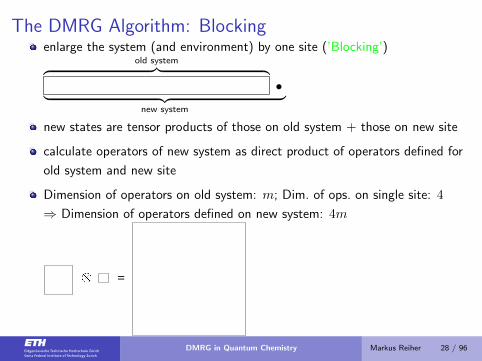
The DMRG Algorithm: Blockingenlarge the system (and environment) by one site (’Blocking’)
old system︷ ︸︸ ︷•︸ ︷︷ ︸
new system
new states are tensor products of those on old system + those on new site
calculate operators of new system as direct product of operators defined for
old system and new site
Dimension of operators on old system: m; Dim. of ops. on single site: 4
⇒ Dimension of operators defined on new system: 4m =
DMRG in Quantum Chemistry Markus Reiher 28 / 96
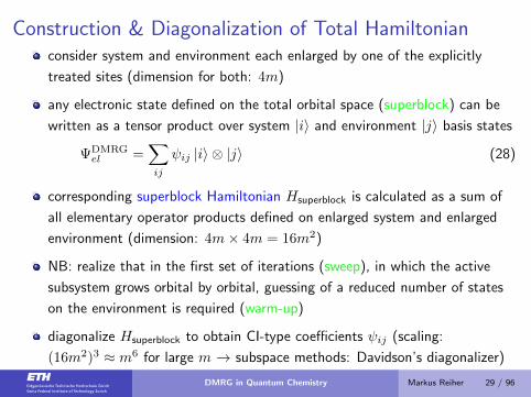
Construction & Diagonalization of Total Hamiltonianconsider system and environment each enlarged by one of the explicitly
treated sites (dimension for both: 4m)
any electronic state defined on the total orbital space (superblock) can be
written as a tensor product over system |i〉 and environment |j〉 basis states
ΨDMRGel =
∑ij
ψij |i〉 ⊗ |j〉 (28)
corresponding superblock Hamiltonian Hsuperblock is calculated as a sum of
all elementary operator products defined on enlarged system and enlarged
environment (dimension: 4m× 4m = 16m2)
NB: realize that in the first set of iterations (sweep), in which the active
subsystem grows orbital by orbital, guessing of a reduced number of states
on the environment is required (warm-up)
diagonalize Hsuperblock to obtain CI-type coefficients ψij (scaling:
(16m2)3 ≈ m6 for large m → subspace methods: Davidson’s diagonalizer)
DMRG in Quantum Chemistry Markus Reiher 29 / 96
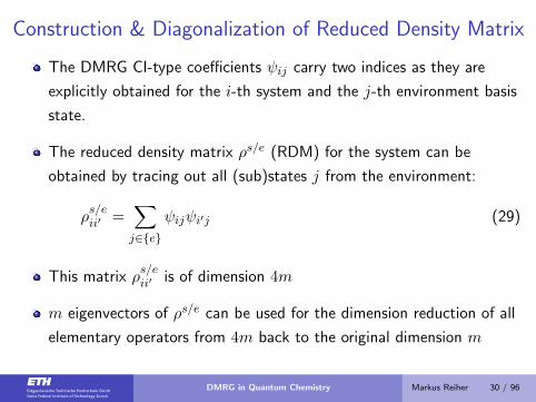
Construction & Diagonalization of Reduced Density Matrix
The DMRG CI-type coefficients ψij carry two indices as they are
explicitly obtained for the i-th system and the j-th environment basis
state.
The reduced density matrix ρs/e (RDM) for the system can be
obtained by tracing out all (sub)states j from the environment:
ρs/eii′ =
∑j∈{e}
ψijψi′j (29)
This matrix ρs/eii′ is of dimension 4m
m eigenvectors of ρs/e can be used for the dimension reduction of all
elementary operators from 4m back to the original dimension m
DMRG in Quantum Chemistry Markus Reiher 30 / 96
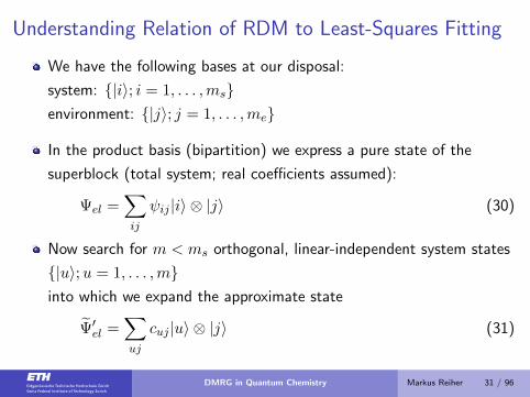
Understanding Relation of RDM to Least-Squares Fitting
We have the following bases at our disposal:
system: {|i〉; i = 1, . . . ,ms}environment: {|j〉; j = 1, . . . ,me}
In the product basis (bipartition) we express a pure state of the
superblock (total system; real coefficients assumed):
Ψel =∑ij
ψij |i〉 ⊗ |j〉 (30)
Now search for m < ms orthogonal, linear-independent system states
{|u〉;u = 1, . . . ,m}into which we expand the approximate state
Ψ′el =∑uj
cuj |u〉 ⊗ |j〉 (31)
DMRG in Quantum Chemistry Markus Reiher 31 / 96
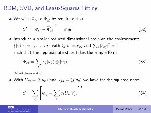
RDM, SVD, and Least-Squares Fitting
We wish Ψel ≈ Ψ′el by requiring that
S′ =∣∣∣Ψel − Ψ′el
∣∣∣2 = min (32)
Introduce a similar reduced-dimensional basis on the environment:
{|v〉; v = 1, . . . ,m} with 〈j|v〉 = cvj and∑
j |cvj |2 = 1
such that the approximate state takes the simple form
Ψel =∑k
ck|uk〉 ⊗ |vk〉 (33)
(Schmidt decomposition)
With Uik = 〈i|uk〉 and Vjk = 〈j|vk〉 we have for the squared norm
S =∑ij
[ψij −
∑k
ckUikVjk
]2
(34)
DMRG in Quantum Chemistry Markus Reiher 32 / 96
RDM, SVD, and Least-Squares Fitting
Here, we recognize the similarity to the least-squares fitting
problem in linear algebra!
Hence, we may use singular value decomposition (SVD) of a
rectangular matrix to minimize S → factorize ψ = (ψij):
ψ = U ·D · V T (35)
The matrix U = (Uik) is orthogonal and of dimension ms ×ms.
The matrix V = (Vjk) is column-orthogonal and of dimension
me ×ms.
D is an ms-dimensional diagonal matrix and contains the singular
values of ψ (assume ms ≤ me, otherwise consider ψT ).
DMRG in Quantum Chemistry Markus Reiher 33 / 96
RDM, SVD, and Least-Squares Fitting
The m largest diagonal elements of D are the desired coefficients ck
and the corresponding column vectors of U and V are the desired
|uk〉 and |vk〉.But how can one make the connection to the RDM?
Consider the von Neumann density operator for the superblock
ρ = |Ψel〉〈Ψel|(30)=∑ii′jj′
ψijψi′j′ |i〉〈i′| ⊗ |j〉〈j′| (36)
reduced density operator from tracing out the enviroment states
ρs = Treρ =∑j′′
∑ii′jj′
ψijψi′j′ |i〉〈i′|〈j′′|j〉〈j′|j′′〉 (37)
=∑ii′j
ψijψi′j |i〉〈i′| (38)
DMRG in Quantum Chemistry Markus Reiher 34 / 96
RDM, SVD, and Least-Squares Fitting
The RDM is then obtained as
ρs = ψ · ψT with (ρs)ii′ =∑j
ψijψi′j (39)
for which we can insert the SVD
ρs = ψ · ψT (35)= (UDV T ) · (V DUT ) = U ·D2 · UT (40)
Hence, U diagonalizes ρs and thus its eigenvalues D2ii are related to
the coefficients ck of the Schmidt decomposition !
Thus, instead of calculating the SVD, one can diagonalize ρs to
obtain the ck =√D2kk from the m highest eigenvalues of D2 and the
corresponding eigenvectors |uk〉.I.e., the larger the eigenvalue D2
ii, the better represents |ui〉 the
system part of the superblock state
DMRG in Quantum Chemistry Markus Reiher 35 / 96
RDM, SVD, and Least-Squares Fitting
Accuracy of approximation can be measured by the truncation error ε
ε = 1−m∑k=1
D2kk (41)
O. Legeza, J. Roder, B. A. Hess, Phys. Rev. B 67 (2003) 125114
This transfers to the accuracy of an observable O as follows
|〈O〉Ψel − 〈O〉Ψel | = |Tr(Oρs)− Tr(Oρs)| =
∣∣∣∣∣ms∑
i=m+1
OiiD2ii
∣∣∣∣∣≤
ms∑i=m+1
|Oii|D2ii ≤ max
i>m|Oii|
ms∑i=m+1
D2ii
= maxi>m|Oii|ε (42)
J. Roder, PhD Thesis, University of Erlangen, 2003
DMRG in Quantum Chemistry Markus Reiher 36 / 96
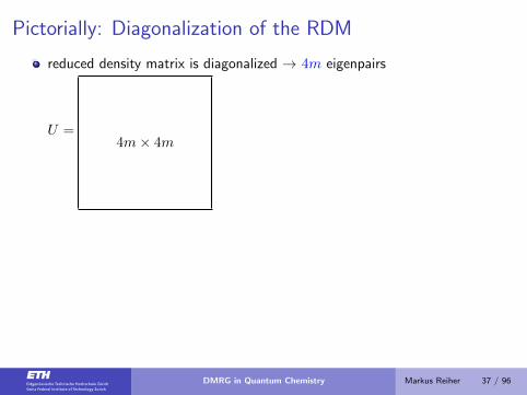
Pictorially: Diagonalization of the RDM
reduced density matrix is diagonalized → 4m eigenpairs
U =4m× 4m
DMRG in Quantum Chemistry Markus Reiher 37 / 96
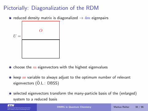
Pictorially: Diagonalization of the RDM
reduced density matrix is diagonalized → 4m eigenpairs
U =
O
choose the m eigenvectors with the highest eigenvalues
keep m variable to always adjust to the optimum number of relevant
eigenvectors (O.L.: DBSS)
selected eigenvectors transform the many-particle basis of the (enlarged)
system to a reduced basis
DMRG in Quantum Chemistry Markus Reiher 38 / 96
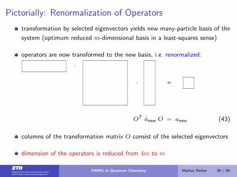
Pictorially: Renormalization of Operators
transformation by selected eigenvectors yields new many-particle basis of the
system (optimum reduced m-dimensional basis in a least-squares sense)
operators are now transformed to the new basis, i.e. renormalized:
.
.
=
OT anew O = anew (43)
columns of the transformation matrix O consist of the selected eigenvectors
dimension of the operators is reduced from 4m to m
DMRG in Quantum Chemistry Markus Reiher 39 / 96
Features of the DMRG AlgorithmDMRG is a CAS approach!
DMRG iterations increase AS orbital by orbital until the environment is
completely absorbed into the system.
Then, the iteration direction is reversed to optimize the environment
representation.
This defines a ’linear’ algorithm, and explains why the orbital ordering can
be important (convergence to local minima possible!).
G. Moritz, B. A. Hess, M. Reiher, J. Chem. Phys. 2005 122 024107
It was thought that DMRG is therefore only beneficial for
pseudo-one-dimensional molecules.
DMRG state is a superposition of FCI-type basis states.
An FCI/CAS solution can be converged; but the basis cannot be completely
known if DMRG shall be efficient
DMRG in Quantum Chemistry Markus Reiher 40 / 96
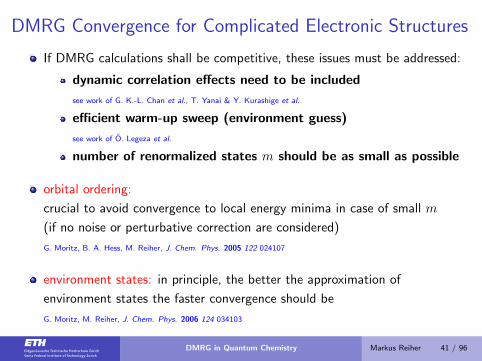
DMRG Convergence for Complicated Electronic Structures
If DMRG calculations shall be competitive, these issues must be addressed:
dynamic correlation effects need to be included
see work of G. K.-L. Chan et al., T. Yanai & Y. Kurashige et al.
efficient warm-up sweep (environment guess)
see work of O. Legeza et al.
number of renormalized states m should be as small as possible
orbital ordering:
crucial to avoid convergence to local energy minima in case of small m
(if no noise or perturbative correction are considered)
G. Moritz, B. A. Hess, M. Reiher, J. Chem. Phys. 2005 122 024107
environment states: in principle, the better the approximation of
environment states the faster convergence should be
G. Moritz, M. Reiher, J. Chem. Phys. 2006 124 034103
DMRG analysis: decomposition of DMRG states in Slater determinant basis
G. Moritz, M. Reiher, J. Chem. Phys. 2007 126 244109
DMRG in Quantum Chemistry Markus Reiher 41 / 96
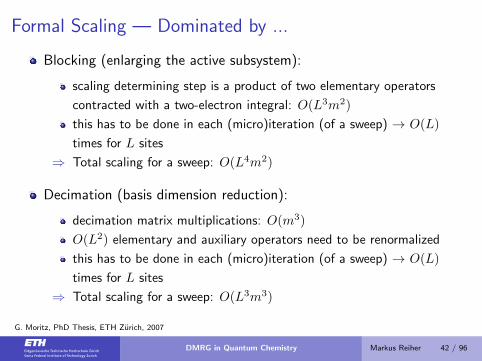
Formal Scaling — Dominated by ...
Blocking (enlarging the active subsystem):
scaling determining step is a product of two elementary operators
contracted with a two-electron integral: O(L3m2)
this has to be done in each (micro)iteration (of a sweep) → O(L)
times for L sites
⇒ Total scaling for a sweep: O(L4m2)
Decimation (basis dimension reduction):
decimation matrix multiplications: O(m3)
O(L2) elementary and auxiliary operators need to be renormalized
this has to be done in each (micro)iteration (of a sweep) → O(L)
times for L sites
⇒ Total scaling for a sweep: O(L3m3)
G. Moritz, PhD Thesis, ETH Zurich, 2007
DMRG in Quantum Chemistry Markus Reiher 42 / 96
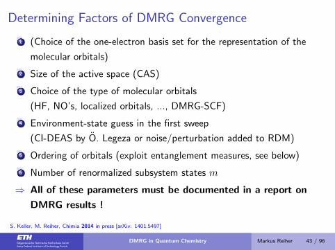
Determining Factors of DMRG Convergence
1 (Choice of the one-electron basis set for the representation of the
molecular orbitals)
2 Size of the active space (CAS)
3 Choice of the type of molecular orbitals
(HF, NO’s, localized orbitals, ..., DMRG-SCF)
4 Environment-state guess in the first sweep
(CI-DEAS by O. Legeza or noise/perturbation added to RDM)
5 Ordering of orbitals (exploit entanglement measures, see below)
6 Number of renormalized subsystem states m
⇒ All of these parameters must be documented in a report on
DMRG results !
S. Keller, M. Reiher, Chimia 2014 in press [arXiv: 1401.5497]
DMRG in Quantum Chemistry Markus Reiher 43 / 96
Lecture 2
Second-Generation DMRG: Matrix Product and Tensor Network
States
1 New Parametrization of the Electronic Wave Function: Tensor
Network States (TNS)
2 Matrix Product States (MPSs) and Matrix Product Operators
(MPOs)
3 Parameters that Determine DMRG Accuracy
DMRG in Quantum Chemistry Markus Reiher 44 / 96
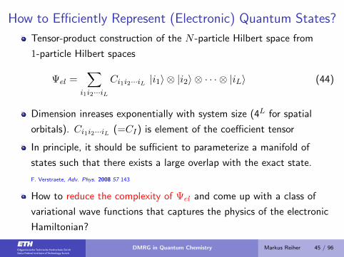
How to Efficiently Represent (Electronic) Quantum States?
Tensor-product construction of the N -particle Hilbert space from
1-particle Hilbert spaces
Ψel =∑
i1i2···iL
Ci1i2···iL |i1〉 ⊗ |i2〉 ⊗ · · · ⊗ |iL〉 (44)
Dimension inreases exponentially with system size (4L for spatial
orbitals). Ci1i2···iL (=CI) is element of the coefficient tensor
In principle, it should be sufficient to parameterize a manifold of
states such that there exists a large overlap with the exact state.
F. Verstraete, Adv. Phys. 2008 57 143
How to reduce the complexity of Ψel and come up with a class of
variational wave functions that captures the physics of the electronic
Hamiltonian?
DMRG in Quantum Chemistry Markus Reiher 45 / 96
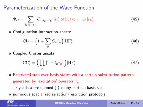
Parameterization of the Wave Function
Ψel =∑
i1i2···iL
Ci1i2···iL |i1〉 ⊗ |i2〉 ⊗ · · · ⊗ |iL〉 (45)
Configuration Interaction ansatz
|CI〉 =(
1 +∑µ
Cµτµ
)|HF〉 (46)
Coupled Cluster ansatz
|CC〉 =(∏
µ
[1 + tµτµ])|HF〉 (47)
Restricted sum over basis states with a certain substitution pattern
generated by ’excitation’ operator τµ
→ yields a pre-defined (!) many-particle basis set
numerous specialized selection/restriction protocols
DMRG in Quantum Chemistry Markus Reiher 46 / 96
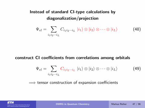
Instead of standard CI-type calculations by
diagonalization/projection
Ψel =∑
i1i2···iL
Ci1i2···iL |i1〉 ⊗ |i2〉 ⊗ · · · ⊗ |iL〉 (48)
construct CI coefficients from correlations among orbitals
Ψel =∑
i1i2···iL
Ci1i2···iL |i1〉 ⊗ |i2〉 ⊗ · · · ⊗ |iL〉 (49)
=⇒ tensor construction of expansion coefficients
DMRG in Quantum Chemistry Markus Reiher 47 / 96
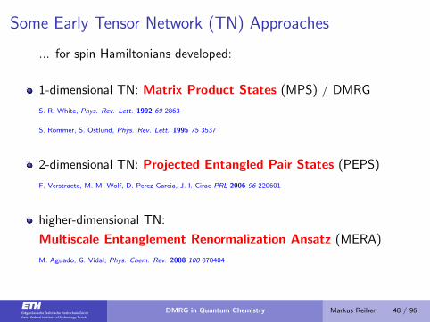
Some Early Tensor Network (TN) Approaches
... for spin Hamiltonians developed:
1-dimensional TN: Matrix Product States (MPS) / DMRG
S. R. White, Phys. Rev. Lett. 1992 69 2863
S. Rommer, S. Ostlund, Phys. Rev. Lett. 1995 75 3537
2-dimensional TN: Projected Entangled Pair States (PEPS)
F. Verstraete, M. M. Wolf, D. Perez-Garcia, J. I. Cirac PRL 2006 96 220601
higher-dimensional TN:
Multiscale Entanglement Renormalization Ansatz (MERA)
M. Aguado, G. Vidal, Phys. Chem. Rev. 2008 100 070404
DMRG in Quantum Chemistry Markus Reiher 48 / 96
MPS & DMRG
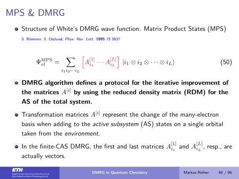
Structure of White’s DMRG wave function: Matrix Product States (MPS)
S. Rommer, S. Ostlund, Phys. Rev. Lett. 1995 75 3537
ΨMPSel =
∑i1i2···iL
[A
[1]i1· · ·A[L]
iL
]|i1 ⊗ i2 ⊗ · · · ⊗ iL〉 (50)
DMRG algorithm defines a protocol for the iterative improvement of
the matrices A[i] by using the reduced density matrix (RDM) for the
AS of the total system.
Transformation matrices A[i] represent the change of the many-electron
basis when adding to the active subsystem (AS) states on a single orbital
taken from the environment.
In the finite-CAS DMRG, the first and last matrices A[1]i1
and A[L]iL
, resp., are
actually vectors.
DMRG in Quantum Chemistry Markus Reiher 49 / 96
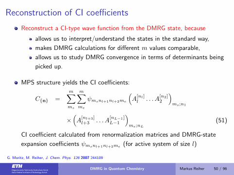
Reconstruction of CI coefficients
Reconstruct a CI-type wave function from the DMRG state, because
allows us to interpret/understand the states in the standard way,
makes DMRG calculations for different m values comparable,
allows us to study DMRG convergence in terms of determinants being
picked up.
MPS structure yields the CI coefficients:
C{n} =
m∑ms
m∑me
ψmsnl+1nl+2me
(A
[nl]l . . . A
[n2]2
)ms;n1
×(A
[nl+3]l+3 . . . A
[nL−1]L−1
)me;nL
(51)
CI coefficient calculated from renormalization matrices and DMRG-state
expansion coefficients ψmsnl+1nl+2me (for active system of size l)
G. Moritz, M. Reiher, J. Chem. Phys. 126 2007 244109
K. Boguslawski, K. H. Marti, M. Reiher, J. Chem. Phys. 134 2011 224101DMRG in Quantum Chemistry Markus Reiher 50 / 96
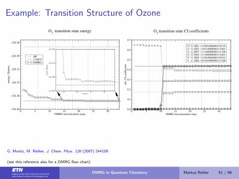
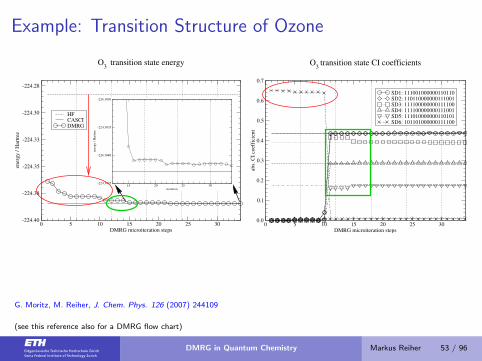
Example: Transition Structure of Ozone
0 5 10 15 20 25 30DMRG microiteration steps
-224.40
-224.38
-224.35
-224.33
-224.30
-224.28
ener
gy
/ H
artr
ee
HFCASCIDMRG
O3
transition state energy
15 20 25 30iteration
-224.3845
-224.3840
-224.3835
-224.3830
ener
gy
/ H
artr
ee
0 5 10 15 20 25 30DMRG microiteration steps
0.0
0.1
0.2
0.3
0.4
0.5
0.6
0.7
abs.
CI
coef
fici
ent
SD1: 111001000000110110SD2: 110110000000111001SD3: 111100000000111100SD4: 111100000000111001SD5: 111010000000110101SD6: 101101000000111100
O3
transition state CI coefficients
G. Moritz, M. Reiher, J. Chem. Phys. 126 (2007) 244109
(see this reference also for a DMRG flow chart)
DMRG in Quantum Chemistry Markus Reiher 51 / 96
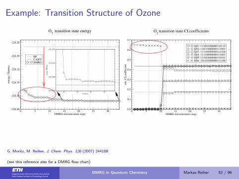
Example: Transition Structure of Ozone
0 5 10 15 20 25 30DMRG microiteration steps
-224.40
-224.38
-224.35
-224.33
-224.30
-224.28
ener
gy
/ H
artr
ee
HFCASCIDMRG
O3
transition state energy
15 20 25 30iteration
-224.3845
-224.3840
-224.3835
-224.3830
ener
gy
/ H
artr
ee
0 5 10 15 20 25 30DMRG microiteration steps
0.0
0.1
0.2
0.3
0.4
0.5
0.6
0.7
abs.
CI
coef
fici
ent
SD1: 111001000000110110SD2: 110110000000111001SD3: 111100000000111100SD4: 111100000000111001SD5: 111010000000110101SD6: 101101000000111100
O3
transition state CI coefficients
G. Moritz, M. Reiher, J. Chem. Phys. 126 (2007) 244109
(see this reference also for a DMRG flow chart)
DMRG in Quantum Chemistry Markus Reiher 52 / 96
Example: Transition Structure of Ozone
0 5 10 15 20 25 30DMRG microiteration steps
-224.40
-224.38
-224.35
-224.33
-224.30
-224.28
ener
gy
/ H
artr
ee
HFCASCIDMRG
O3
transition state energy
15 20 25 30iteration
-224.3845
-224.3840
-224.3835
-224.3830
ener
gy
/ H
artr
ee
0 5 10 15 20 25 30DMRG microiteration steps
0.0
0.1
0.2
0.3
0.4
0.5
0.6
0.7
abs.
CI
coef
fici
ent
SD1: 111001000000110110SD2: 110110000000111001SD3: 111100000000111100SD4: 111100000000111001SD5: 111010000000110101SD6: 101101000000111100
O3
transition state CI coefficients
G. Moritz, M. Reiher, J. Chem. Phys. 126 (2007) 244109
(see this reference also for a DMRG flow chart)
DMRG in Quantum Chemistry Markus Reiher 53 / 96
SR-CAS Approach
Our 2007 scheme could only reconstruct FCI from DMRG wave functions for
which a FCI calculation was also possible.
Cure: Sampling-Reconstruction Complete-Active-Space algorithm:
Monte Carlo scheme for sampling configurations
Only the most important configurations are kept.
The accuracy is easily controlled by a completeness measure COM:
COM = 1−∑
I∈{sample}
C2I (52)
K. Boguslawski, K. H. Marti, M. Reiher, J. Chem. Phys. 134 (2011) 224101
DMRG in Quantum Chemistry Markus Reiher 54 / 96
Derivation of MPS Structure of DMRG Wave Function
The CI coefficient tensor Ci1i2···iL
Ψel =∑
i1i2···iL
Ci1i2···iL |i1〉 ⊗ |i2〉 ⊗ · · · ⊗ |iL〉
≡∑
i1i2···iL
Ci1i2···iL |i1, i2, . . . iL〉 ≡∑I
CIΦI (53)
can be decomposed by sequential SVDs, which clarifies the MPS structure
of the DMRG wave function.
Consider a DMRG state function with the first orbital (from the left) in
the AS and (L− 1) orbitals in the environment,
ΨDMRGel =
∑i1,j
ψi1j |i1〉 ⊗ |j〉 with j = (i2 . . . iL) (54)
Hence, the coefficient tensor Ci1i2···iL is approximated by a matrix ψi1j.
DMRG in Quantum Chemistry Markus Reiher 55 / 96
Derivation of MPS Structure of DMRG Wave Function
ψi1j is of dimension (m×mL−1) and can be subjected to an SVD
Ci1i2···iL → ψi1j = ψi1(i2...iL) =
r1∑a1
Ui1a1 Da1a1 VTa1(i2...iL)
≡r1∑a1
Ui1a1 Ca1i2...iL (55)
with the rank r1 ≤ m. Now, change notation:
a) matrix U is written as a collection of row vectors Ai1 with entries
Ai1a1= Ui1a1 .
b) coefficient tensor Ca1i2...iL is ordered as a matrix ψ(a1i2)(i3...iL) of
dimension (r1 ·m×mL−2)
DMRG in Quantum Chemistry Markus Reiher 56 / 96
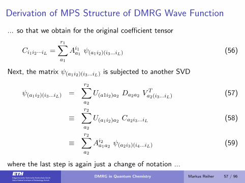
Derivation of MPS Structure of DMRG Wave Function
... so that we obtain for the original coefficient tensor
Ci1i2···iL =
r1∑a1
Ai1a1ψ(a1i2)(i3...iL) (56)
Next, the matrix ψ(a1i2)(i3...iL) is subjected to another SVD
ψ(a1i2)(i3...iL) =
r2∑a2
U(a1i2)a2Da2a2 V
Ta2(i3...iL) (57)
≡r2∑a2
U(a1i2)a2Ca2i3...iL (58)
≡r2∑a2
Ai2a1a2ψ(a2i3)(i4...iL) (59)
where the last step is again just a change of notation ...
DMRG in Quantum Chemistry Markus Reiher 57 / 96
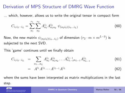
Derivation of MPS Structure of DMRG Wave Function
... which, however, allows us to write the original tensor in compact form
Ci1i2···iL =
r1∑a1
r2∑a2
Ai1a1Ai2a1a2
ψ(a2i3)(i4...iL) (60)
Now, the new matrix ψ(a2i3)(i4...iL) of dimension (r2 ·m×mL−3) is
subjected to the next SVD.
This ’game’ continues until we finally obtain
Ci1i2···iL =∑a1...aL
Ai1a1Ai2a1a2
. . . AiL−1aL−2aL−1A
iLaL−1
(61)
= Ai1Ai2 · · ·AiL−1AiL (62)
where the sums have been interpreted as matrix multiplications in the last
step.
DMRG in Quantum Chemistry Markus Reiher 58 / 96
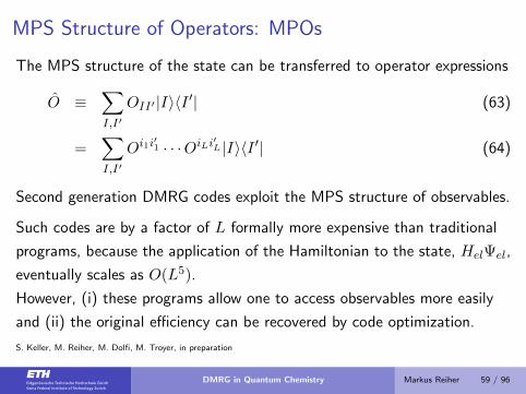
MPS Structure of Operators: MPOs
The MPS structure of the state can be transferred to operator expressions
O ≡∑I,I′
OII′ |I〉〈I ′| (63)
=∑I,I′
Oi1i′1 · · ·OiLi′L |I〉〈I ′| (64)
Second generation DMRG codes exploit the MPS structure of observables.
Such codes are by a factor of L formally more expensive than traditional
programs, because the application of the Hamiltonian to the state, HelΨel,
eventually scales as O(L5).
However, (i) these programs allow one to access observables more easily
and (ii) the original efficiency can be recovered by code optimization.
S. Keller, M. Reiher, M. Dolfi, M. Troyer, in preparation
DMRG in Quantum Chemistry Markus Reiher 59 / 96
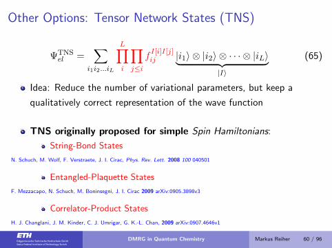
Other Options: Tensor Network States (TNS)
ΨTNSel =
∑i1i2...iL
L∏i
∏j≤i
fI[i]I[j]ij |i1〉 ⊗ |i2〉 ⊗ · · · ⊗ |iL〉︸ ︷︷ ︸
|I〉
(65)
Idea: Reduce the number of variational parameters, but keep a
qualitatively correct representation of the wave function
TNS originally proposed for simple Spin Hamiltonians:
String-Bond States
N. Schuch, M. Wolf, F. Verstraete, J. I. Cirac, Phys. Rev. Lett. 2008 100 040501
Entangled-Plaquette States
F. Mezzacapo, N. Schuch, M. Boninsegni, J. I. Cirac 2009 arXiv:0905.3898v3
Correlator-Product States
H. J. Changlani, J. M. Kinder, C. J. Umrigar, G. K.-L. Chan, 2009 arXiv:0907.4646v1
DMRG in Quantum Chemistry Markus Reiher 60 / 96
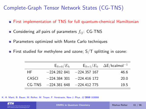
Complete-Graph Tensor Network States (CG-TNS)
First implementation of TNS for full quantum-chemical Hamiltonian
Considering all pairs of parameters fij : CG-TNS
Parameters optimized with Monte Carlo techniques
First studied for methylene and ozone; S/T splitting in ozone:
ES=0/Eh ES=1/Eh ∆E/kcalmol−1
HF −224.282 841 −224.357 167 46.6
CASCI −224.384 301 −224.416 172 20.0
CG-TNS −224.381 648 −224.412 775 19.5
K. H. Marti, B. Bauer, M. Reiher, M. Troyer, F. Verstraete, New J. Phys. 12 2010 103008
DMRG in Quantum Chemistry Markus Reiher 61 / 96
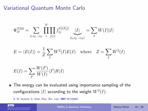
Variational Quantum Monte Carlo
ΨTNSel =
∑i1i2...iN
N∏i
∏j≤i
fI[i]I[j]ij |I〉︸︷︷︸
|i1i2...iN 〉
=∑I
W (I)|I〉
E = 〈E(I)〉 =1
Z
∑I
W 2(I)E(I) where Z =∑I
W 2(I)
E(I) =∑I′
W (I ′)
W (I)〈I ′|H|I〉
The energy can be evaluated using importance sampling of the
configurations |I〉 according to the weight W 2(I).
A. W. Sandvik, G. Vidal, Phys. Rev. Lett. 2007 99 220602
DMRG in Quantum Chemistry Markus Reiher 62 / 96
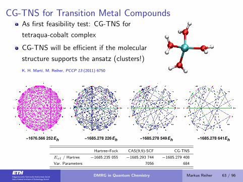
CG-TNS for Transition Metal CompoundsAs first feasibility test: CG-TNS for
tetraqua-cobalt complex
CG-TNS will be efficient if the molecular
structure supports the ansatz (clusters!)
K. H. Marti, M. Reiher, PCCP 13 (2011) 6750
Eh
Eh
Eh
Eh
−1676.566 252 −1685.278 226 −1685.278 549 −1685.278 641
Hartree–Fock CAS(9,9)-SCF CG-TNS
Eel / Hartree −1685.235 055 −1685.293 744 −1685.279 408
Var. Parameters 7056 684
DMRG in Quantum Chemistry Markus Reiher 63 / 96
Lecture 3
Results of Actual Quantum-Chemical Calculations
(taken from our group)
1 DMRG for Compact Strongly Correlated Molecules: Transition Metal
Complexes
2 DMRG Spin Density
3 Concepts of Quantum Information Theory for Electronic Structures
and Chemical Bonding
DMRG in Quantum Chemistry Markus Reiher 64 / 96
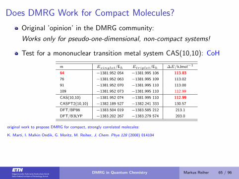
Does DMRG Work for Compact Molecules?
Original ’opinion’ in the DMRG community:
Works only for pseudo-one-dimensional, non-compact systems!
Test for a mononuclear transition metal system CAS(10,10): CoH
m Esinglet/Eh Etriplet/Eh ∆E/kJmol−1
64 −1381.952 054 −1381.995 106 113.03
76 −1381.952 063 −1381.995 109 113.02
91 −1381.952 070 −1381.995 110 113.00
109 −1381.952 073 −1381.995 110 112.99
CAS(10,10) −1381.952 074 −1381.995 110 112.99
CASPT2(10,10) −1382.189 527 −1382.241 333 130.57
DFT/BP86 −1383.504 019 −1383.585 212 213.1
DFT/B3LYP −1383.202 267 −1383.279 574 203.0
original work to propose DMRG for compact, strongly correlated molecules:
K. Marti, I. Malkin Ondik, G. Moritz, M. Reiher, J. Chem. Phys 128 (2008) 014104
DMRG in Quantum Chemistry Markus Reiher 65 / 96
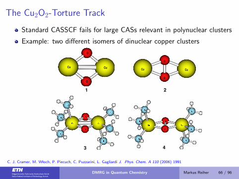
The Cu2O2-Torture Track
Standard CASSCF fails for large CASs relevant in polynuclear clusters
Example: two different isomers of dinuclear copper clusters
C. J. Cramer, M. W loch, P. Piecuch, C. Puzzarini, L. Gagliardi J. Phys. Chem. A 110 (2006) 1991
DMRG in Quantum Chemistry Markus Reiher 66 / 96
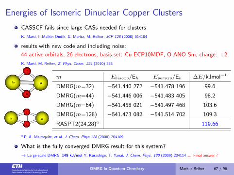
Energies of Isomeric Dinuclear Copper Clusters
CASSCF fails since large CASs needed for clusters
K. Marti, I. Malkin Ondik, G. Moritz, M. Reiher, JCP 128 (2008) 014104
results with new code and including noise:
44 active orbitals, 26 electrons, basis set: Cu ECP10MDF, O ANO-Sm, charge: +2
K. Marti, M. Reiher, Z. Phys. Chem. 224 (2010) 583
Cu
O
O
Cu
Cu
O
O
Cu
m Ebisoxo/Eh Eperoxo/Eh ∆E/kJmol−1
DMRG(m=32) −541.440 272 −541.478 196 99.6
DMRG(m=44) −541.446 006 −541.483 405 98.2
DMRG(m=64) −541.458 021 −541.497 468 103.6
DMRG(m=128) −541.473 082 −541.514 702 109.3
RASPT2(24,28)a 119.66
aP. A. Malmqvist, et al. J. Chem. Phys 128 (2008) 204109
What is the fully converged DMRG result for this system?
→ Large-scale DMRG: 149 kJ/mol Y. Kurashige, T. Yanai, J. Chem. Phys. 130 (2009) 234114 ... Final answer ?
DMRG in Quantum Chemistry Markus Reiher 67 / 96
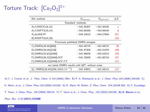
Torture Track: [Cu2O2]2+
Ref.,method Ebisoxo Eperoxo ∆E
’Standard’ methods
A),CASSCF(16,14) −541.50307 −541.50345 1
A),CASPT2(16,14) −542.06208 −542.06435 6
A),bs-B3LYP −544.19419 −544.27844 221
B),RASPT2(24,28) 120
Previously published DMRG energies
C),DMRG(26,44)[800] −541.46779 −541.49731 78
D),DMRG(26,44)[128] −541.47308 −541.51470 109
E),DMRG(32,62)[2400] −541.96839 −542.02514 149
F),DMRG(28,32)[2048]-SCF −541.76659 −541.80719 107
F),DMRG(28,32)[2048]-SCF/CT 113
our latest DMRG results with QIT, without noise
G), DMRG(26,44)[256/1024/10−5] −541.53853 −541.58114 112
A) C. J. Cramer et al., J. Phys. Chem. A 110 (2006) 1991; B) P. A. Malmqvist et al., J. Chem. Phys 128 (2008) 204109; C)
K. Marti, et al., J. Chem. Phys 128 (2008) 014104; D) K. Marti, M. Reiher, Z. Phys. Chem. 224 (20109 583; E) Y. Kurashige,
T. Yanai, J. Chem. Phys. 130 (2009) 234114; F) T. Yanai et al., J. Chem. Phys. 132 (2010) 024105; G) G. Barcza et al.,
Phys. Rev. A 83 (2011) 012508
DMRG in Quantum Chemistry Markus Reiher 68 / 96
Analysis of Spin Density Distributions
with DMRG
DMRG in Quantum Chemistry Markus Reiher 69 / 96
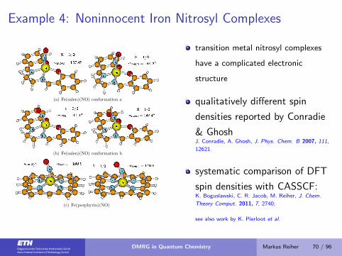
Example 4: Noninnocent Iron Nitrosyl Complexes
(a) Fe(salen)(NO) conformation a
(b) Fe(salen)(NO) conformation b
(c) Fe(porphyrin)(NO)
transition metal nitrosyl complexes
have a complicated electronic
structure
qualitatively different spin
densities reported by Conradie
& GhoshJ. Conradie, A. Ghosh, J. Phys. Chem. B 2007, 111,
12621.
systematic comparison of DFT
spin densities with CASSCF:K. Boguslawski, C. R. Jacob, M. Reiher, J. Chem.
Theory Comput. 2011, 7, 2740;
see also work by K. Pierloot et al.
DMRG in Quantum Chemistry Markus Reiher 70 / 96
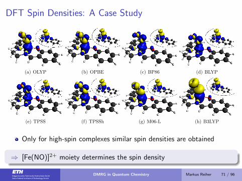
DFT Spin Densities: A Case Study
(a) OLYP (b) OPBE (c) BP86 (d) BLYP
(e) TPSS (f) TPSSh (g) M06-L (h) B3LYP
Only for high-spin complexes similar spin densities are obtained
⇒ [Fe(NO)]2+ moiety determines the spin density
DMRG in Quantum Chemistry Markus Reiher 71 / 96
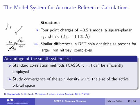
The Model System for Accurate Reference Calculations
zyx
Fe
N
O
�
dpcdpc
dpcdpc
Structure:
Four point charges of −0.5 e model a square-planar
ligand field (ddp = 1.131 A)
⇒ Similar differences in DFT spin densities as present for
larger iron nitrosyl complexes
Advantage of the small system size:
Standard correlation methods (CASSCF, . . .) can be efficiently
employed
Study convergence of the spin density w.r.t. the size of the active
orbital space
K. Boguslawski, C. R. Jacob, M. Reiher, J. Chem. Theory Comput. 2011, 7, 2740.
DMRG in Quantum Chemistry Markus Reiher 72 / 96
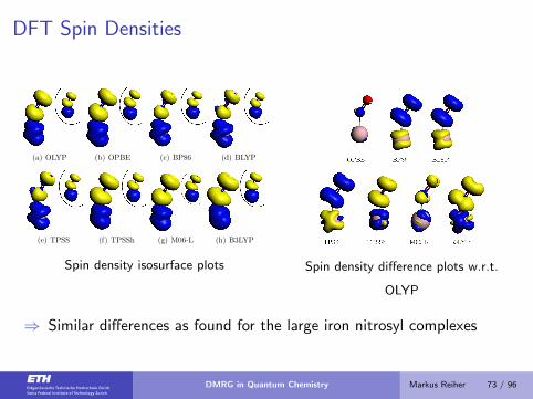
DFT Spin Densities
(a) OLYP (b) OPBE (c) BP86 (d) BLYP
(e) TPSS (f) TPSSh (g) M06-L (h) B3LYP
Spin density isosurface plots Spin density difference plots w.r.t.
OLYP
⇒ Similar differences as found for the large iron nitrosyl complexes
DMRG in Quantum Chemistry Markus Reiher 73 / 96
Reference Spin Densities
from Standard Electron Correlation Methods
DMRG in Quantum Chemistry Markus Reiher 74 / 96
Reference Spin Densities from CASSCF Calculations
Defining the active orbital space:
Minimal active space: Fe 3d- and both NO π∗-orbitals ⇒ CAS(7,7)
Consider also both NO π-orbitals ⇒ CAS(11,9)
Additional shell of Fe d-orbitals (double-shell orbitals) is gradually
included ⇒ CAS(11,11) to CAS(11,14)
Include one ligand σ-orbital and the antibonding σ∗-orbital upon the
CAS(11,11) ⇒ CAS(13,13)
⇒ Analyze convergence of spin density w.r.t. the dimension of the active
orbital space
DMRG in Quantum Chemistry Markus Reiher 75 / 96
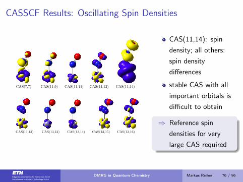
CASSCF Results: Oscillating Spin Densities
CAS(7,7) CAS(11,9) CAS(11,11) CAS(11,12) CAS(11,14)
CAS(11,13) CAS(13,13) CAS(13,14) CAS(13,15) CAS(13,16)
CAS(11,14): spin
density; all others:
spin density
differences
stable CAS with all
important orbitals is
difficult to obtain
⇒ Reference spin
densities for very
large CAS required
DMRG in Quantum Chemistry Markus Reiher 76 / 96
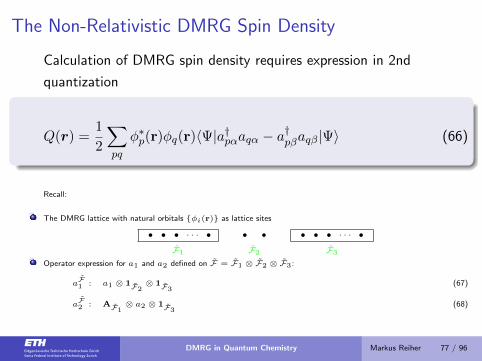
The Non-Relativistic DMRG Spin Density
Calculation of DMRG spin density requires expression in 2nd
quantization
Q(r) =1
2
∑pq
φ∗p(r)φq(r)〈Ψ|a†pαaqα − a†pβaqβ|Ψ〉 (66)
Recall:
The DMRG lattice with natural orbitals {φi(r)} as lattice sites
• • • · · · • • • • • • · · · •
F1 F2 F3
Operator expression for a1 and a2 defined on F = F1 ⊗ F2 ⊗ F3:
aF1 : a1 ⊗ 1F2
⊗ 1F3(67)
aF2 : AF1
⊗ a2 ⊗ 1F3(68)
Operator product:
aF1 · a
F2 =
(a1 ·AF1
)⊗ (a2)⊗
(1F3
)
DMRG in Quantum Chemistry Markus Reiher 77 / 96
DMRG Spin Densities — Measures of Convergence
Qualitative convergence measure: spin density difference plots
Quantitative convergence measure:
∆abs =
∫|ρs
1(r)− ρs2(r)|dr < 0.005 (69)
∆sq =
√∫|ρs
1(r)− ρs2(r)|2dr < 0.001 (70)
Quantitative convergence measure: quantum fidelity Fm1,m2
Fm1,m2 = |〈Ψ(m1)|Ψ(m2)〉|2 (71)
⇒ Reconstructed CI expansion of DMRG wave function can be used!
K. Boguslawski, K. H. Marti, M. Reiher, J. Chem. Phys. 2011, 134, 224101.
DMRG in Quantum Chemistry Markus Reiher 78 / 96
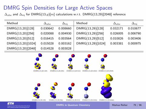
DMRG Spin Densities for Large Active Spaces∆abs and ∆sq for DMRG(13,y)[m] calculations w.r.t. DMRG(13,29)[2048] reference
Method ∆abs ∆sq Method ∆abs ∆sq
DMRG(13,20)[128] 0.030642 0.008660 DMRG(13,29)[128] 0.032171 0.010677
DMRG(13,20)[256] 0.020088 0.004930 DMRG(13,29)[256] 0.026005 0.006790
DMRG(13,20)[512] 0.016415 0.003564 DMRG(13,29)[512] 0.010826 0.003406
DMRG(13,20)[1024] 0.015028 0.003162 DMRG(13,29)[1024] 0.003381 0.000975
DMRG(13,20)[2048] 0.014528 0.003028
DMRG(13,20;128) DMRG(13,20;256) DMRG(13,20;512) DMRG(13,20;1024) DMRG(13,20;2048)
DMRG(13,29;128) DMRG(13,29;256) DMRG(13,29;512) DMRG(13,29;1024) DMRG(13,29;2048)
DMRG in Quantum Chemistry Markus Reiher 79 / 96
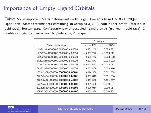
Importance of Empty Ligand Orbitals
Table: Some important Slater determinants with large CI weights from DMRG(13,29)[m]
Upper part: Slater determinants containing an occupied dx2−y2 -double-shell orbital (marked in
bold face). Bottom part: Configurations with occupied ligand orbitals (marked in bold face). 2:
doubly occupied; a: α-electron; b: β-electron; 0: empty.
CI weight
Slater determinant m = 128 m = 1024
b2b222a0a0000000 0000000 a 00000 0.003 252 0.003 991
bb2222aa00000000 0000000 a 00000 −0.003 226 −0.003 611
222220ab00000000 0000000 a 00000 −0.002 762 −0.003 328
ba2222ab00000000 0000000 a 00000 0.002 573 0.003 022
b2a222a0b0000000 0000000 a 00000 −0.002 487 −0.003 017
202222ab00000000 0000000 a 00000 0.002 405 0.002 716
b222a2a0b0000000 0000000 0 0000a 0.010 360 0.011 558
22b2a2a0a0000000 0000000 0 b0000 0.009 849 0.011 366
22b2a2a0b0000000 0000000 0 a0000 −0.009 532 −0.011 457
b2222aab00000000 0000000 0 0000a −0.009 490 −0.010 991
a2222baa00000000 0000000 0 0000b −0.009 014 −0.010 017
b2b222a0a0000000 0000000 0 0a000 0.008 820 0.010 327
DMRG in Quantum Chemistry Markus Reiher 80 / 96
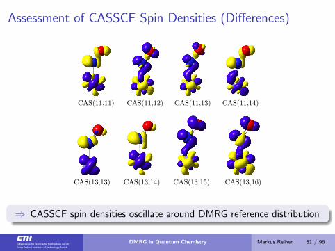
Assessment of CASSCF Spin Densities (Differences)
CAS(11,11) CAS(11,12) CAS(11,13) CAS(11,14)
CAS(13,13) CAS(13,14) CAS(13,15) CAS(13,16)
⇒ CASSCF spin densities oscillate around DMRG reference distribution
DMRG in Quantum Chemistry Markus Reiher 81 / 96
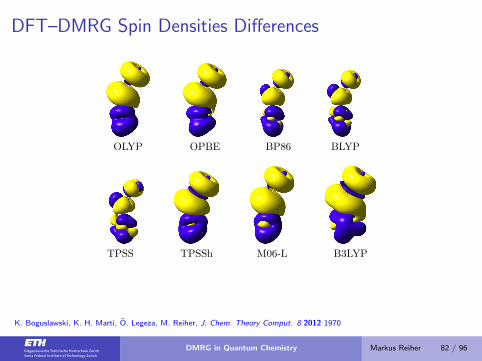
DFT–DMRG Spin Densities Differences
OLYP OPBE BP86 BLYP
TPSS TPSSh M06-L B3LYP
K. Boguslawski, K. H. Marti, O. Legeza, M. Reiher, J. Chem. Theory Comput. 8 2012 1970
DMRG in Quantum Chemistry Markus Reiher 82 / 96
Analyzing DMRG and correlated wave functions
with concepts from quantum information theory
DMRG in Quantum Chemistry Markus Reiher 83 / 96
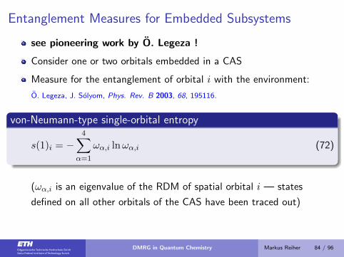
Entanglement Measures for Embedded Subsystems
see pioneering work by O. Legeza !
Consider one or two orbitals embedded in a CAS
Measure for the entanglement of orbital i with the environment:
O. Legeza, J. Solyom, Phys. Rev. B 2003, 68, 195116.
von-Neumann-type single-orbital entropy
s(1)i = −4∑
α=1
ωα,i lnωα,i (72)
(ωα,i is an eigenvalue of the RDM of spatial orbital i — states
defined on all other orbitals of the CAS have been traced out)
DMRG in Quantum Chemistry Markus Reiher 84 / 96
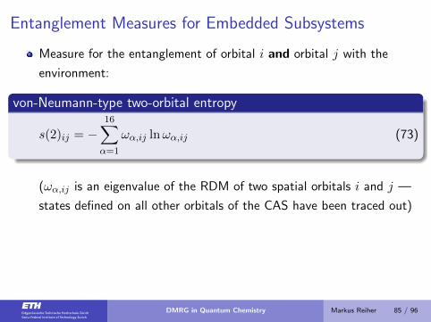
Entanglement Measures for Embedded Subsystems
Measure for the entanglement of orbital i and orbital j with the
environment:
von-Neumann-type two-orbital entropy
s(2)ij = −16∑α=1
ωα,ij lnωα,ij (73)
(ωα,ij is an eigenvalue of the RDM of two spatial orbitals i and j —
states defined on all other orbitals of the CAS have been traced out)
DMRG in Quantum Chemistry Markus Reiher 85 / 96
Entanglement Measures for Embedded Subsystems
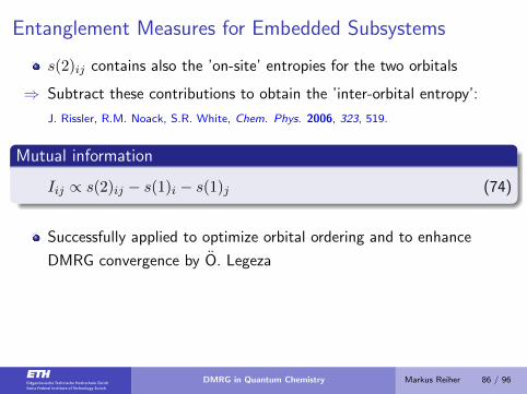
s(2)ij contains also the ’on-site’ entropies for the two orbitals
⇒ Subtract these contributions to obtain the ’inter-orbital entropy’:
J. Rissler, R.M. Noack, S.R. White, Chem. Phys. 2006, 323, 519.
Mutual information
Iij ∝ s(2)ij − s(1)i − s(1)j (74)
Successfully applied to optimize orbital ordering and to enhance
DMRG convergence by O. Legeza
DMRG in Quantum Chemistry Markus Reiher 86 / 96
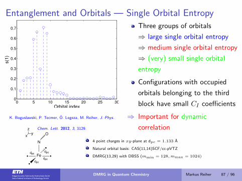
Entanglement and Orbitals — Single Orbital Entropy
0 5 10 15 20 25 300
0.1
0.2
0.3
0.4
0.5
0.6
0.7
Orbital index
s(1
)
K. Boguslawski, P. Tecmer, O. Legeza, M. Reiher, J. Phys.
Chem. Lett. 2012, 3, 3129.
Three groups of orbitals
⇒ large single orbital entropy
⇒ medium single orbital entropy
⇒ (very) small single orbital
entropy
Configurations with occupied
orbitals belonging to the third
block have small CI coefficients
⇒ Important for dynamic
correlation
zyx
Fe
N
O
�
dpcdpc
dpcdpc
4 point charges in xy-plane at dpc = 1.133 A
Natural orbital basis: CAS(11,14)SCF/cc-pVTZ
DMRG(13,29) with DBSS (mmin = 128,mmax = 1024)
DMRG in Quantum Chemistry Markus Reiher 87 / 96
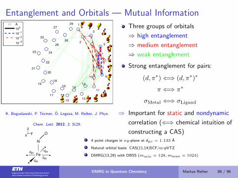
Entanglement and Orbitals — Mutual Information
1
3
5
7
9
11
1315
17
19
21
23
25
27
29
2
4
6
8
10
12
1416
18
20
22
24
26
28
A
100
10−1
10−2
10−3
K. Boguslawski, P. Tecmer, O. Legeza, M. Reiher, J. Phys.
Chem. Lett. 2012, 3, 3129.
Three groups of orbitals
⇒ high entanglement
⇒ medium entanglement
⇒ weak entanglement
Strong entanglement for pairs:
(d, π∗)⇐⇒ (d, π∗)∗
π ⇐⇒ π∗
σMetal ⇐⇒ σLigand
⇒ Important for static and nondynamic
correlation (⇐⇒ chemical intuition of
constructing a CAS)
zyx
Fe
N
O
�
dpcdpc
dpcdpc
4 point charges in xy-plane at dpc = 1.133 A
Natural orbital basis: CAS(11,14)SCF/cc-pVTZ
DMRG(13,29) with DBSS (mmin = 128,mmax = 1024)
DMRG in Quantum Chemistry Markus Reiher 88 / 96
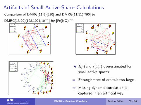
Artifacts of Small Active Space CalculationsComparison of DMRG(11,9)[220] and DMRG(11,11)[790] to
DMRG(13,29)[128,1024,10−5] for [Fe(NO)]2+
1
3
5
7
9
2
4
6
8
A
100
10−1
10−2
10−3
1
3
5
7
9
11
2
4
6
8
10
A
100
10−1
10−2
10−3
1
3
5
7
9
11
1315
17
19
21
23
25
27
29
2
4
6
8
10
12
1416
18
20
22
24
26
28
A
100
10−1
10−2
10−3
Iij (and s(1)i) overestimated for
small active spaces
⇒ Entanglement of orbitals too large
⇒ Missing dynamic correlation is
captured in an artificial way
DMRG in Quantum Chemistry Markus Reiher 89 / 96
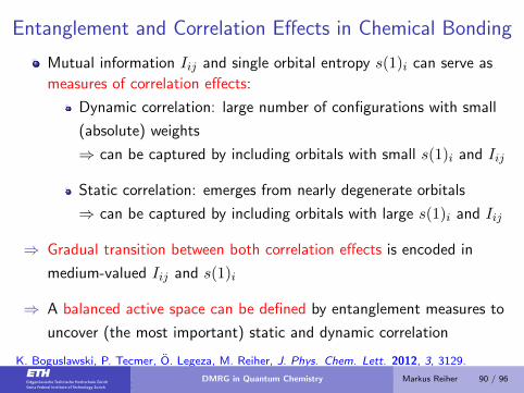
Entanglement and Correlation Effects in Chemical Bonding
Mutual information Iij and single orbital entropy s(1)i can serve as
measures of correlation effects:
Dynamic correlation: large number of configurations with small
(absolute) weights
⇒ can be captured by including orbitals with small s(1)i and Iij
Static correlation: emerges from nearly degenerate orbitals
⇒ can be captured by including orbitals with large s(1)i and Iij
⇒ Gradual transition between both correlation effects is encoded in
medium-valued Iij and s(1)i
⇒ A balanced active space can be defined by entanglement measures to
uncover (the most important) static and dynamic correlation
K. Boguslawski, P. Tecmer, O. Legeza, M. Reiher, J. Phys. Chem. Lett. 2012, 3, 3129.
K. Boguslawski, P. Tecmer, G. Barcza, O. Legeza, M. Reiher, J. Chem. Theory Comput. 9 2013
2959–2973 [arxiv: 1303.7207]
DMRG in Quantum Chemistry Markus Reiher 90 / 96
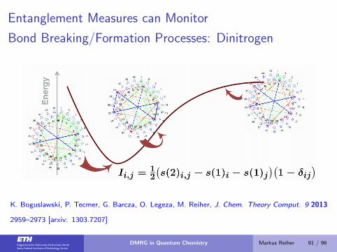
Entanglement Measures can Monitor
Bond Breaking/Formation Processes: Dinitrogen
K. Boguslawski, P. Tecmer, G. Barcza, O. Legeza, M. Reiher, J. Chem. Theory Comput. 9 2013
2959–2973 [arxiv: 1303.7207]
DMRG in Quantum Chemistry Markus Reiher 91 / 96
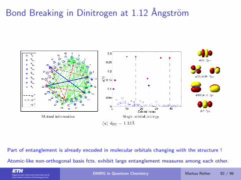
Bond Breaking in Dinitrogen at 1.12 Angstrom
Part of entanglement is already encoded in molecular orbitals changing with the structure !
Atomic-like non-orthogonal basis fcts. exhibit large entanglement measures among each other.
DMRG in Quantum Chemistry Markus Reiher 92 / 96
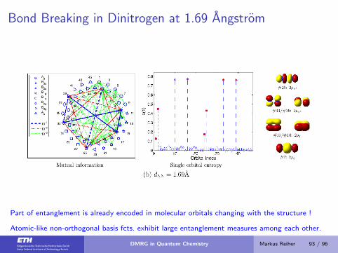
Bond Breaking in Dinitrogen at 1.69 Angstrom
Part of entanglement is already encoded in molecular orbitals changing with the structure !
Atomic-like non-orthogonal basis fcts. exhibit large entanglement measures among each other.
DMRG in Quantum Chemistry Markus Reiher 93 / 96
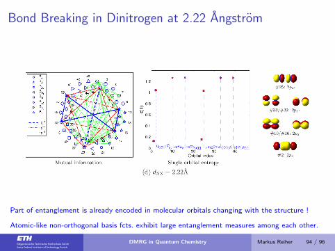
Bond Breaking in Dinitrogen at 2.22 Angstrom
Part of entanglement is already encoded in molecular orbitals changing with the structure !
Atomic-like non-orthogonal basis fcts. exhibit large entanglement measures among each other.
DMRG in Quantum Chemistry Markus Reiher 94 / 96
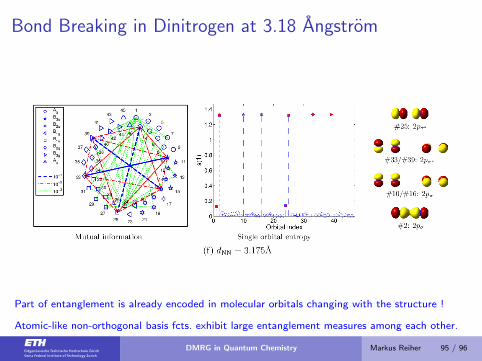
Bond Breaking in Dinitrogen at 3.18 Angstrom
Part of entanglement is already encoded in molecular orbitals changing with the structure !
Atomic-like non-orthogonal basis fcts. exhibit large entanglement measures among each other.
DMRG in Quantum Chemistry Markus Reiher 95 / 96
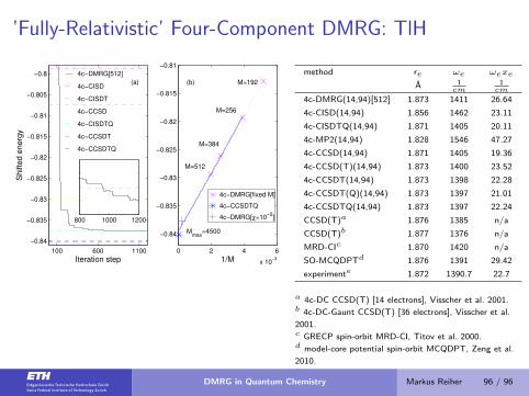
’Fully-Relativistic’ Four-Component DMRG: TlH
100 600 1100
−0.84
−0.835
−0.83
−0.825
−0.82
−0.815
−0.81
−0.805
−0.8 4c−DMRG[512]
4c−CISD
4c−CISDT
4c−CCSD
4c−CISDTQ
4c−CCSDT
4c−CCSDTQ
(a)
Iteration step
Sh
ifte
d e
ne
rgy
800 1000 1200
0 2 4 6
x 10−3
−0.84
−0.835
−0.83
−0.825
−0.82
−0.815
−0.81
4c−DMRG[fixed M]
4c−CCSDTQ
4c−DMRG[χ=10−5
]
1/M
Mmax
=4500
M=512
M=384
M=256
M=192(b)
method re ωe ωexe
A 1cm
1cm
4c-DMRG(14,94)[512] 1.873 1411 26.64
4c-CISD(14,94) 1.856 1462 23.11
4c-CISDTQ(14,94) 1.871 1405 20.11
4c-MP2(14,94) 1.828 1546 47.27
4c-CCSD(14,94) 1.871 1405 19.36
4c-CCSD(T)(14,94) 1.873 1400 23.52
4c-CCSDT(14,94) 1.873 1398 22.28
4c-CCSDT(Q)(14,94) 1.873 1397 21.01
4c-CCSDTQ(14,94) 1.873 1397 22.24
CCSD(T)a 1.876 1385 n/a
CCSD(T)b 1.877 1376 n/a
MRD-CIc 1.870 1420 n/a
SO-MCQDPTd 1.876 1391 29.42
experimente 1.872 1390.7 22.7
a 4c-DC CCSD(T) [14 electrons], Visscher et al. 2001.b 4c-DC-Gaunt CCSD(T) [36 electrons], Visscher et al.
2001.c GRECP spin-orbit MRD-CI, Titov et al. 2000.d model-core potential spin-orbit MCQDPT, Zeng et al.
2010.e experimental data.
S. Knecht, O. Legeza, M. Reiher, J. Chem. Phys 140 (2014) 041101
DMRG in Quantum Chemistry Markus Reiher 96 / 96