econstor www.econstor.eu

Der Open-Access-Publikationsserver der ZBW – Leibniz-Informationszentrum WirtschaftThe Open Access Publication Server of the ZBW – Leibniz Information Centre for Economics

Standard-Nutzungsbedingungen:

Die Dokumente auf EconStor dürfen zu eigenen wissenschaftlichenZwecken und zum Privatgebrauch gespeichert und kopiert werden.

Sie dürfen die Dokumente nicht für öffentliche oder kommerzielleZwecke vervielfältigen, öffentlich ausstellen, öffentlich zugänglichmachen, vertreiben oder anderweitig nutzen.

Sofern die Verfasser die Dokumente unter Open-Content-Lizenzen(insbesondere CC-Lizenzen) zur Verfügung gestellt haben sollten,gelten abweichend von diesen Nutzungsbedingungen die in der dortgenannten Lizenz gewährten Nutzungsrechte.

Terms of use:

Documents in EconStor may be saved and copied for yourpersonal and scholarly purposes.

You are not to copy documents for public or commercialpurposes, to exhibit the documents publicly, to make thempublicly available on the internet, or to distribute or otherwiseuse the documents in public.

If the documents have been made available under an OpenContent Licence (especially Creative Commons Licences), youmay exercise further usage rights as specified in the indicatedlicence.

zbw Leibniz-Informationszentrum WirtschaftLeibniz Information Centre for Economics

Angelopoulos, Konstantinos; Jiang, Wei; Malley, Jim

Working Paper

Fiscal Multipliers in a Two-Sector Search andMatching Model

CESifo Working Paper, No. 5197

Provided in Cooperation with:Ifo Institute – Leibniz Institute for Economic Research at the University ofMunich

Suggested Citation: Angelopoulos, Konstantinos; Jiang, Wei; Malley, Jim (2015) : FiscalMultipliers in a Two-Sector Search and Matching Model, CESifo Working Paper, No. 5197

This Version is available at:http://hdl.handle.net/10419/107378

Fiscal Multipliers in a Two-Sector Search and Matching Model

Konstantinos Angelopoulos Wei Jiang

James Malley

CESIFO WORKING PAPER NO. 5197 CATEGORY 6: FISCAL POLICY, MACROECONOMICS AND GROWTH

JANUARY 2015

An electronic version of the paper may be downloaded • from the SSRN website: www.SSRN.com • from the RePEc website: www.RePEc.org

• from the CESifo website: Twww.CESifo-group.org/wp T

CESifo Working Paper No. 5197

Fiscal Multipliers in a Two-Sector Search and Matching Model

Abstract This paper evaluates the effects of policy interventions on sectoral labour markets and the aggregate economy in a business cycle model with search and matching frictions. We extend the canonical model by including capital-skill complementarity in production, labour markets with skilled and unskilled workers and on-the-job-learning (OJL) within and across skill types. We first find that, the model does a good job at matching the cyclical properties of sectoral employment and the wage-skill premium. We next find that vacancy subsidies for skilled and unskilled jobs lead to output multipliers which are greater than unity with OJL and less than unity without OJL. In contrast, the positive output effects from cutting skilled and unskilled income taxes are close to zero. Finally, we find that the sectoral and aggregate effects of vacancy subsidies do not depend on whether they are financed via public debt or distorting taxes.

JEL-Code: E240, E320, J630, J640, J680.

Keywords: fiscal multipliers, sectoral labour markets, search and matching.

Konstantinos Angelopoulos University of Glasgow / UK

k.angelopoulos@lbss.gla.ac.uk

Wei Jian* University of Kent / UK

w.jiang@kent.ac.uk

James Malley University of Glasgow / UK

j.malley@lbss.gla.ac.uk

*corresponding author January 25, 2015 We would like to thank Pedro Gomes, Amanda Gosling, Miguel León-Ledesma, Mathan Satchi, Fabien Postel-Vinay and participants at the Computing in Economics and Finance, 2014 conference in Oslo and the University of Kent Workshop on Labour Market, Public Policy and the Business Cycle for helpful comments and suggestions.

1 Introduction

Equilibrium unemployment models with search and matching frictions havebeen extensively used in macroeconomic analyses of unemployment (see e.g.Shimer (2010) and Rogerson and Shimer (2011) for an analytical overviewof this research). Among other extensions, this literature has consideredthe importance of both di¤erences in workers� skills and the potential forskill erosion due to unemployment (see e.g. Cahuc et al. (2006), Krauseand Lubik (2006 and 2010), Dolado et al. (2009), Hagedorn et al. (2010),Doppelt (2014) and Laureys (2014)). In this paper, we contribute to thisliterature by examining unemployment over the business cycle in an economywith fragmented labour markets for University educated (or skilled) and non-University educated (or unskilled) workers, when the production structureis characterised by capital-skill complementarity and workers�productivitydecreases with unemployment.Our interest in labour markets and unemployment for skilled versus un-

skilled workers is motivated by empirical evidence on the importance of thedi¤erences between these two labour markets, regarding both wage and em-ployment rates. We summarise some key di¤erences using quarterly data forthe U.S. over the period of 1992-2011 for sectoral employment and 1979-2003for wage inequality.1

First, the literature on the skill premium has demonstrated that thereare signi�cant di¤erences in the wages across the two sectors. In particular,wage inequality between skilled and unskilled labour has increased in recentdecades to its highest levels in a century (see e.g. Goldin and Katz (2008)and Acemoglu and Autor (2011) for a discussion of longer time series andhistorical data). This is demonstrated in the subplot (1,1) of Figure 1, whichplots the skill premium, de�ned as the ratio of skilled to unskilled wage, usingthe quarterly series from Castro and Coen-Pirani (2008).Second, wage inequality varies in business cycle frequencies, although

less than output and is not strongly correlated with output (see also e.g.Lindquist (2004) and Pourpourides (2011)). This is captured in subplot(2,1) which shows HP-�ltered output and the skill premium. In particular,the relative to output volatility of the skill premium is 0:87 and its output

1The data sources for the skilled and unskilled wage data (1979-2003) are from thedataset of Castro and Coen-Pirani (2008). Sectoral employment/unemployment data(1992-2011) are from the Current Population Survey, Table A-4. We use data on theemployment status of the civilian population 25 years and over by educational attainment(see www.bls.gov/webapps/legacy/cpsatab4.htm). Finally, per capita quarterly outputdata (1979-2011) are from the U.S. NIPA.

2

correlation is 0:086.[Figure 1 here]

Third, employment di¤ers signi�cantly between the two sectors. For ex-ample, the data in subplot (1,2), show that unemployment is twice as high forunskilled compared with skilled workers.2 Moreover, as demonstrated in sub-plot (2,2), unskilled employment is more volatile than skilled, although bothclosely track cyclical output. In particular, the volatility of the HP-�lteredunskilled employment is 1:8 times higher than that of skilled workers, whereastheir output correlations are about 0:93.The literature has documented further di¤erences between the skilled and

unskilled sectors. Cahuc et al. (2006) �nd that skilled workers have higherbargaining power, while Pissarides (1994), Acemoglu (2001) and Krause andLubik (2006 and 2010) suggest that the �ow cost of posting a vacancy ishigher in �good�jobs. Moreover, in business cycle frequencies, there is notmuch movement between the skilled and unskilled sectors.In light of the above, we build a business cycle model with search and

matching frictions that lead to sectoral unemployment. To capture the aboveempirical observations, we �rst assume that unskilled workers cannot becomeskilled. Instead, skilled workers work in skilled jobs and, if unemployed,search for employment in the skilled sector. Similarly, unskilled workers workin unskilled jobs, and if unemployed, search for employment in the unskilledsector. Second, we assume that the production structure allows for skill-biased technical change and, in particular, is characterised by capital-skillcomplementarity. This setup has been shown to explain key characteris-tics of the skill premium in the data, both in terms of its evolution overthe past several decades (see e.g. Katz and Murphy (1992), Krusell et al.(2000) and He (2012)) as well as over the business cycle (Lindquist (2004)and Pourpourides (2011)). The search and matching mechanism for employ-ment creation that we employ follows the benchmark Mortensen-Pissaridesframework with the wage being determined via Nash bargaining. Moreover,our setup allows for di¤erentiation between the two labour markets, such asdi¤erences in relative bargaining power, job separation rates and job postingcosts to re�ect the empirical observations outlined above.Motivated by theories of labour augmenting technical progress driven by

on-the-job learning (OJL), we allow skilled and unskilled workers�productiv-ities to be positive functions of employment. Alternatively, since the sectoralproductivities are decreasing functions of unemployment, they can equiva-lently capture skill erosion due to not working. We consider two possibilities

2Fallick and Fleischman (2004), Hagedorn et al. (2010), and Pilossoph (2012) alsodocument higher job separation rates for unskilled versus skilled workers.

3

for OJL where both skill types learn from their own and the other skill type.The �rst follows the literature that proposes learning-by-doing (LBD) as

a property of the production technology at the aggregate level and generatesknowledge spillovers. It thus works as an external e¤ect for the individual(see e.g. Romer (1986) and Barro and Sala-i-Martin (1994)). In this casethe workers� labour productivity depends on average employment, so thatLBD is taken as given at the level of the workers. The second follows moreclosely the literature on skill erosion that is due to unemployment (see e.g.Laureys (2014) and Doppelt (2014)). In this instance we allow the workersof each type to internalise the e¤ect of their own employment on their labourproductivity. However, we maintain the assumption that the employment ofthe other worker type is taken as given.The model is calibrated to match the steady-state of aggregate and sec-

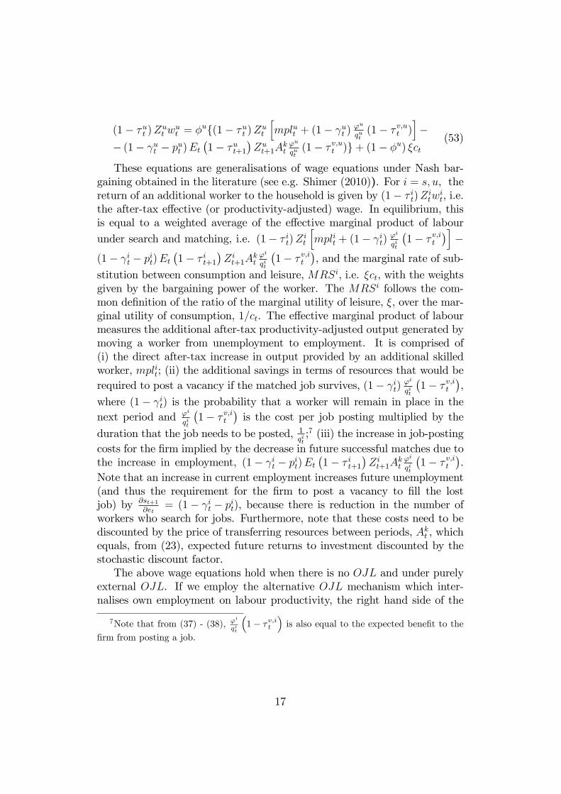
toral labour market data in the U.S., following the calibration strategy inShimer (2010). We �nd that the calibration does a good job at matching thesecond moments in the sectoral labour market data. In particular, the modelpredicts a volatility for unskilled employment that is about twice as big asthat of skilled employment. Moreover, it predicts a series for the skill pre-mium whose volatility is less than output and its correlation with output isaround zero. Consistent with the results in Shimer, the model under predictsquantitatively the volatility of employment, but the gap is not very big. Inparticular, the model variants considered predict an employment volatilitywhich ranges from 69% to 81% of the volatility of employment in the data,whereas in the canonical models, e.g. Shimer (2010), this ratio is typicallyabout 25%. Since the model with and without OJL gives a relatively similar�t to the data, we present results below for policy interventions using bothspeci�cations.Our policy analysis evaluates the e¤ects of temporary interventions on

the sectoral labour markets and the aggregate economy. We consider vacancysubsidies and taxes, since as is demonstrated in Monacelli et al. (2010), pure�scal spending e¤ects on output are trivial and even negative in search andmatching models. We �nd �scal multipliers on output from the subsidesto skilled and unskilled vacancies, which are greater than unity when OJLis external and near unity when it is internal. These large multipliers aredetermined by the crowding-in of private investment, which follows the in-creases in employment and labour productivity. Without OJL, the labourproductivity channel is absent and causes the output multipliers to fall toabout 0.6. In contrast to the vacancy subsidies, the positive output e¤ectsfrom cutting skilled and unskilled income taxes are near zero, irrespectiveof the presence, or model, of OJL. We �nally �nd that the e¤ects of thetwo vacancy subsidies do not depend on whether debt or distorting taxes

4

are used to �nance them. This is particularly good news, and suggests thatthis type of intervention may be useful under the debt restrictions that manygovernments now face in the wake of the �nancial crisis.The rest of the paper is organised as follows. Section 2 sets out the

model structure. Section 3 presents the calibration and cyclical properties ofthe model. Section 4 undertakes the �scal multiplier analysis and Section 5concludes.

2 The model

2.1 Capital-skill complementarity

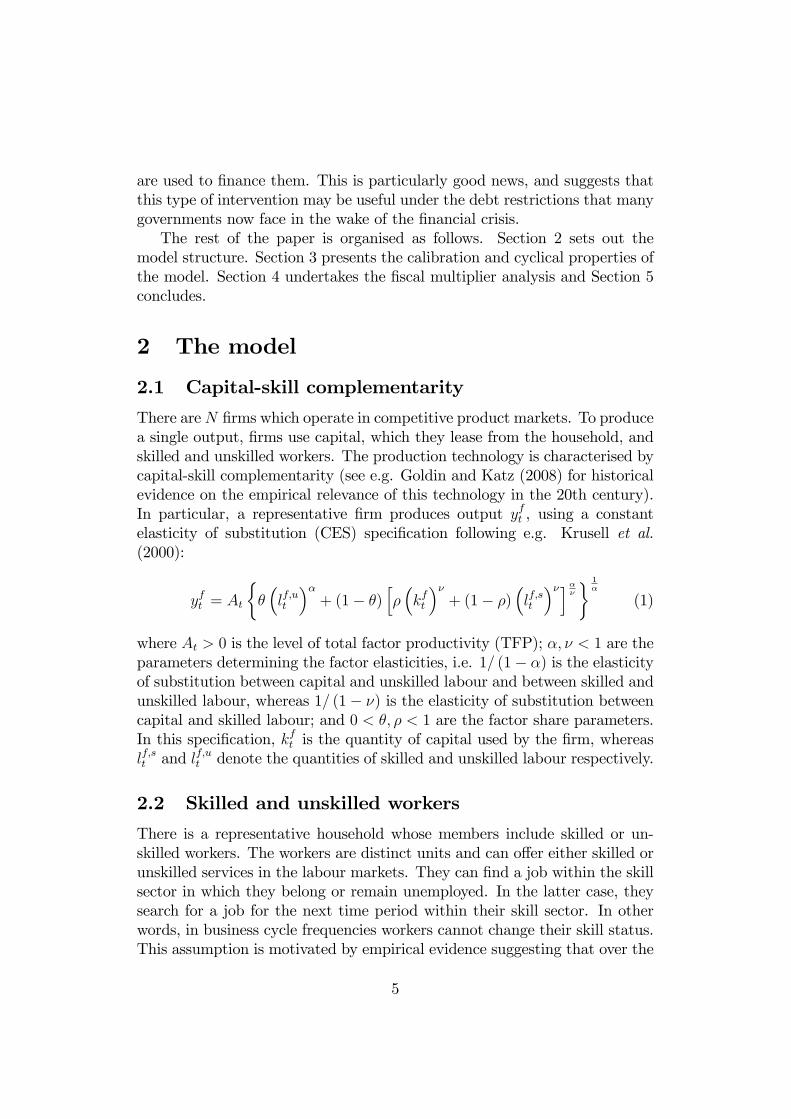
There areN �rms which operate in competitive product markets. To producea single output, �rms use capital, which they lease from the household, andskilled and unskilled workers. The production technology is characterised bycapital-skill complementarity (see e.g. Goldin and Katz (2008) for historicalevidence on the empirical relevance of this technology in the 20th century).In particular, a representative �rm produces output yft , using a constantelasticity of substitution (CES) speci�cation following e.g. Krusell et al.(2000):

yft = At

���lf;ut

��+ (1� �)

h��kft

��+ (1� �)

�lf;st

��i��� 1�

(1)

where At > 0 is the level of total factor productivity (TFP); �; � < 1 are theparameters determining the factor elasticities, i.e. 1= (1� �) is the elasticityof substitution between capital and unskilled labour and between skilled andunskilled labour, whereas 1= (1� �) is the elasticity of substitution betweencapital and skilled labour; and 0 < �; � < 1 are the factor share parameters.In this speci�cation, kft is the quantity of capital used by the �rm, whereaslf;st and lf;ut denote the quantities of skilled and unskilled labour respectively.

2.2 Skilled and unskilled workers

There is a representative household whose members include skilled or un-skilled workers. The workers are distinct units and can o¤er either skilled orunskilled services in the labour markets. They can �nd a job within the skillsector in which they belong or remain unemployed. In the latter case, theysearch for a job for the next time period within their skill sector. In otherwords, in business cycle frequencies workers cannot change their skill status.This assumption is motivated by empirical evidence suggesting that over the

5

business cycle, the share of college educated or skilled population has lowvolatility and is e¤ectively uncorrelated with output. In particular, usingthe data in Acemoglu and Autor (2011), we �nd that the standard deviationof the cyclical component of the skilled population share, relative to that ofoutput, is 0.29, while its correlation with output is -0.23.3 This implies thatskilled workers can either work in skilled jobs or remain unemployed (andsearch for skilled jobs), whereas unskilled workers can either work in un-skilled jobs or remain unemployed (and search for unskilled jobs). Followingthe literature on search frictions and unemployment in macroeconomic DGEmodels since Mertz (1995), we assume that the head of the household makesall decisions on behalf of its members and provides complete consumptioninsurance. In other words, all workers consume the same amount of goods,irrespective of their labour market status, i.e. regardless of whether they areemployed in skilled or unskilled jobs or they are unemployed.The numbers of skilled and unskilled members for the representative

household are denoted as N s and Nu, respectively. The total size of thehousehold is normalised to be N and is thus given as: N = N s + Nu. Therespective population shares of skilled and unskilled members within a house-hold are de�ned as: ns = N s=N and nu = Nu=N . We assume that populationand its composition remain constant.For each skill type of household members, i = s; u, the number of mem-

bers/workers can be further decomposed into employed and unemployedmembers, such that:

N i = N i;et +N i;s

t (2)

where i = s; u for skilled and unskilled labour; and N i;et is the number of

employed members and N i;st is the number of unemployed members, who are

searching for a job. By normalising by N i, we have:

1 = eit + sit (3)

where eit �N i;et

N i is the employment rate and sit �N i;st

N i is the unemploymentrate or the share of workers searching for a job.

2.3 Search and matching

There are two labour markets, for skilled and unskilled workers respectively.Each unemployed worker needs to search for a job in the skilled or unskilled

3This is obtained using annual data for the share of college educated population mea-sured in e¢ ciency units, 1963-2008, from Acemoglu and Autor (2011) and GDP per capitadata from the U.S. National Income and Product Accounts (NIPA). The cyclical compo-nent of the series is obtained using the HP-�lter with a smoothing parameter of 100.

6

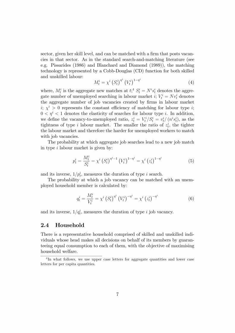
sector, given her skill level, and can be matched with a �rm that posts vacan-cies in that sector. As in the standard search-and-matching literature (seee.g. Pissarides (1986) and Blanchard and Diamond (1989)), the matchingtechnology is represented by a Cobb-Douglas (CD) function for both skilledand unskilled labour:

M it = �i

�Sit��i �

V it

�1��i(4)

where, M it is the aggregate new matches at t;

4 Sit = N isit denotes the aggre-gate number of unemployed searching in labour market i; V i

t = Nvit denotesthe aggregate number of job vacancies created by �rms in labour marketi; �i > 0 represents the constant e¢ ciency of matching for labour type i;0 < �i < 1 denotes the elasticity of searches for labour type i. In addition,we de�ne the vacancy-to-unemployed ratio, zit = V i

t =Sit = vit= (n

isit), as thetightness of type i labour market. The smaller the ratio of zit, the tighterthe labour market and therefore the harder for unemployed workers to matchwith job vacancies.The probability at which aggregate job searches lead to a new job match

in type i labour market is given by:

pit =M i

t

Sit= �i

�Sit��i�1 �

V it

�1��i= �i

�zit�1��i

(5)

and its inverse, 1=pit, measures the duration of type i search.The probability at which a job vacancy can be matched with an unem-

ployed household member is calculated by:

qit =M i

t

V it

= �i�Sit��i �

V it

���i= �i

�zit���i

(6)

and its inverse, 1=qit, measures the duration of type i job vacancy.

2.4 Household

There is a representative household comprised of skilled and unskilled indi-viduals whose head makes all decisions on behalf of its members by guaran-teeing equal consumption to each of them, with the objective of maximisinghousehold welfare.

4In what follows, we use upper case letters for aggregate quantities and lower caseletters for per capita quantities.

7

2.4.1 Problem

The representative household maximises discounted lifetime utility, Ut:

Ut = Et

1Xt=0

�tut (7)

where Et is the conditional expectations operator at period t; and 0 < � <1 denotes the constant rate of time preference. The instantaneous utilityfunction of the household is given by (see e.g. Shimer (2010)):

ut = ln(ct)� ns�est � nu�eut (8)

where � > 0 is the preference parameter that measures the disutility cost ofemployment and ct is the household�s average (or per capita) private con-sumption. As is common in the literature, the disutility cost captures thereduction in the time available for home production when a member �ndsemployment. Hence, the speci�cation in (8) assumes that all members con-sume ct and that if a member is unemployed, her utility is given by ln(ct),whereas if a member is employed, her utility is given by ln(ct) � �i, so thatut measures average utility for the household.The budget constraint of the household is:

ct + it + bt+1 =�rt � � kt (rt � �)

�kt + �t+

+Rbtbt + (1� � st)n

swst estZ

st + (1� �ut )n

uwut eutZ

ut

(9)

where it is household�s average private investment; bt+1 is the value of gov-ernment bonds bought at period t; rt is the gross return to physical capital;� kt is the tax rate on capital income; 0 < � < 1 is the constant depreciationrate of physical capital; kt is the average physical capital held by the house-hold at the beginning of t; �t is average dividends received from the �rms;Rbt =

�1 + rbt

�is the gross return to bonds; � it is the labour income tax; w

it is

the gross wage rate; and Zit represents labour augmenting technology driven

by OJL. This technology positively depends on the level of employment. Al-ternatively, Zi

t can be interpreted as a decreasing function of unemploymentand captures skill erosion due to not working.5 We allow for both skill typesto learn on-the-job from their own and the other skill type.We consider two possibilities for OJL. The �rst follows the literature that

proposes learning-by-doing (LBD) as a property of the production technol-ogy at the aggregate level. This setup generates knowledge spillovers at the

5See, for example, Davis and von Wachter (2011) and Pollack (2013) for the e¤ects ofunemployment on labour productivity and Laureys (2014) and Doppelt (2014) for searchand matching models with skill depreciation due to unemployment.

8

aggregate level which work as an external e¤ect for the individual (see e.g.Romer (1986) and Barro and Sala-i-Martin (1994)). In this case, we allowthe worker�s labour productivity to depend on average employment, so thatLBD (or, alternatively, skill erosion) is taken as given at the level of theworker. This case is represented as follows:

Zst � Zs;x

t = s (est)�s (eut )

1��s (10)

Zut � Zu;x

t = u (est)�u (eut )

1��u (11)

where a bar over a variable refers to average quantities; i > 0 are learningproductivity parameters; and 0 < � i < 1, are the elasticities of OJL withrespect to skilled employment for skilled and unskilled workers.We will proceed with the model solution below using (10) and (11). How-

ever, we will also present and discuss results using a second possibility forthe determination of Zi

t , following more closely the literature on skill erosionthat is due to unemployment (see e.g. Laureys (2014) and Doppelt (2014)).This alternative assumes that workers internalise the e¤ect of employmenton their labour productivity. Hence, in this case we allow the worker of eachtype to internalise the e¤ect of their own employment on their labour pro-ductivity. However, we maintain the assumption that the employment of theother worker type is taken as given:6

Zst � Zs;n

t = s (est)�s (eut )

1��s (12)

Zut � Zu;n

t = u (est)�u (eut )

1��u . (13)

The capital stock evolves according to:

kt+1 = (1� �) kt + ~Akt it (14)

The capital evolution equation allows for an exogenous process, ~Akt , capturingan investment-speci�c technological (IT) change, which has been shown tocontribute to output �uctuations (see e.g. Greenwood et al. (2000), as wellas the changes in the skill premium (see e.g. Krusell et al. (2000), Lindquist(2004), and Pourpourides (2011)). The stochastic process for investment-speci�c technology, ~Akt is:

eAkt+1 = � eAk�1��Ak � eAkt��Ak e"Akt+1 (15)

where eAk > 0; 0 < �Ak < 1; and "Ak

t+1 � iidN�0; (�Ak)

2�.6Note that in both speci�cations examined, labour productivity is increasing and con-

cave with respect to employment and bounded between zero and i, where i = s; u.

9

By using equation (14) and de�ning as Akt � 1~Akt, we can rewrite the

budget constraint of household:

ct + Akt kt+1 + bt+1 = ertkt + �t++Rb

tbt + (1� � st)nswst e

stZ

st + (1� �ut )n

uwut eutZ

ut

(16)

where ert = rt � � kt (rt � �) + Akt (1� �), is the net return to physical capitalafter depreciation and tax. Note that Akt � 1

~Aktmeasures the e¤ective price

of investment, since Akt units of investment are needed to create one unit ofcapital in the next period.Employment for type i = s; u worker evolves according to:

eit+1 = pitsit +�1� it

�eit (17)

where 0 < it < 1 is the rate of job separation for type i labour. Thestochastic process for the job separation rate, it, is:

it+1 =� i�1��gi � it��gi e"git+1 (18)

where i > 0; 0 < �gi < 1; and "gi

t+1 � iidNh0;��ig�2i.

The household�s optimization problem is to choose fct; kt+1; bt+1g1t=0 tomaximise (7) subject to the constraints (3) and (16) taking factor pricesfwst ; wut ; rt; rbtg1t=0; pro�ts f�tg

1t=0; the evolution of employment feitg

1t=0; the

exogenous variables�Akt ;

it

1t=0; policy variables

�� kt ; �

st ; �

ut

1t=0

and initialconditions for k0; b0 as given.

2.4.2 First-order conditions (FOCs)

The recursive form of the household�s problem is:

V (kt; bt; est ; e

ut ) = max

ct;kt+1;bt+1f(ln ct � ns�est � nu�eut )+

+�EtV�kt+1; bt+1; e

st+1; e

ut+1

�g

(19)

where V (:) is the value function. Replacing ct making use of the budgetconstraint (16) gives:

V (kt; bt; est ; e

ut ) = max

kt+1;bt+1[ ln[ertkt � Akt kt+1 � bt+1 + �t +Rb

tbt+

+(1� � st)nswst e

stZ

st + (1� �ut )n

uwut eutZ

ut ]� ns�est � nu�eut+

+�EtV (kt+1; bt+1; est+1; e

ut+1)]:

(20)

The envelope condition for capital stock, kt is:

Vk (kt; bt; est ; e

ut ) =

ertct

(21)

10

and the �rst order condition for kt+1 is:

�EtVk�kt+1; bt+1; e

st+1; e

ut+1

�=Aktct

(22)

which equates the discounted expected marginal bene�t to the marginal costof investment.Finally, substituting the one-period lead of the envelope condition (21)

into the �rst-order condition for capital (22) gives the consumption Euler:

Et

��ctert+1ct+1

�= Akt (23)

which shows that the expected, discounted return on investing in capitalmust equal its price. Note that the return is discounted using the stochasticdiscount factor � ct

ct+1. The envelope condition for government bonds, bt is:

Vb (kt; bt; est ; e

ut ) =

Rbt

ct(24)

and the �rst order condition for bt+1 is:

�EtVb�kt+1; bt+1; e

st+1; e

ut+1

�=1

ct. (25)

Substituting the one-period lead of the envelope condition (24) into the�rst-order condition for government bonds (25) gives the bonds Euler, whichhas a similar interpretation as the Euler for capital:

Et

�ct�1 + rbt+1

�ct+1

!= 1 (26)

The FOCs for the household�s problem are given by (16), (23) and (26).These determine the paths for fct; kt+1; bt+1g1t=0 given exogenous variables�Akt ;

it

1t=0; policy variables

�� kt ; �

st ; �

ut

1t=0; initial conditions, fk0; b0g; and

the paths for variables that are exogenous to the household�s problem, i.e.those determined at the aggregate level,

��t; rt; r

bt ; e

it+1

1t=0and by wage bar-

gaining, fwitg1t=0.

2.5 Firms

There is a representative �rm which leases capital from the household andemploys skilled and unskilled workers to produce a single good, with theobjective of maximising pro�ts.

11

2.5.1 Problem

To hire workers, the �rm needs to post vacancies one period before the jobsare required. In particular, the evolution of the number of workers per skilledtype employed by the �rm is given by the job transition function which linksthe future number of �lled jobs, lf;it+1, to the net hiring, q

itvit, plus the current

stock of �lled jobs, (1� it) lf;it :

lf;it+1 = qitvit +�1� it

�lf;it : (27)

Given that posting vacancies is costly, the pro�t function of the �rm is:

�ft = yft � rtkft � wst l

f;st � (1� � v;st )'

svst � wut lf;ut � (1� � v;ut )'

uvut (28)

where 's; 'u > 0 stand for the constant resource costs of opening a newskilled and unskilled vacancy respectively; and � v;it refer to the vacancy sub-sidies.The employment evolution equations in (27) imply that pro�t maximi-

sation is intertemporal, since expenditure on posting vacancies today willincrease pro�ts tomorrow. Therefore, the objective of the �rm at time pe-riod t = 0 is to maximise the present value of its lifetime pro�ts, which isgiven by:

yf0 � r0kf0 � ws0l

f;s0 � (1� � v;s0 )'

svs0 � wu0 lf;u0 � (1� � v;u0 )'

uvu0+

+Et

1Xt=1

tYi=1

er�1i fyft � rtkft � wst l

f;st � (1� � v;st )'

svst � wut lf;ut �

� (1� � v;ut )'uvut g

(29)

where yf0 and yft are given by the CES production function in (1) at time 0

and t respectively.Since pro�ts are returned to the household, t + 1 returns are converted

to present value terms by the stochastic discount factor from the household�s

optimisation problem, (23). For i = s; u, the �rm choosesnkft ; v

it; l

f;it+1

o1t=0

to maximise (29) subject to (27) , taking factor prices fwit; rtg1t=0; matching

probabilities fqitg1t=0; exogenous job separation rates f itg

1t=0; economic pol-

icy�� v;it1t=0; and initial conditions for flf;i0 g as given. The variable, At is

determined by the following stochastic process:

At+1 = (A)1��A (At)

�A e"At+1 (30)

where A > 0; 0 < �A < 1; and "At+1 � iidN

�0; (�A)

2�.12

2.5.2 First-order conditions

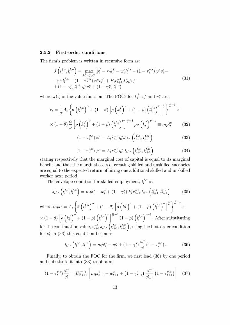
The �rm�s problem is written in recursive form as:

J�lf;st ; lf;ut

�= max

kft ;vst ;v

ut

[yft � rtkft � wst l

f;st � (1� � v;st )'

svst�

�wut lf;ut � (1� � v;ut )'

uvut ] + Eter�1t+1J(qst vst++(1� st) l

f;st ; qut v

ut + (1� ut ) l

f;ut )

(31)

where J(:) is the value function. The FOCs for kft , vst and v

ut are:

rt =1

�At

���lf;ut

��+ (1� �)

h��kft

��+ (1� �)

�lf;st

��i��� 1��1

�

� (1� �)�

�

h��kft

��+ (1� �)

�lf;st

��i���1���kft

���1� mplkt (32)

(1� � v;st )'s = Eter�1t+1qstJlf;s �lf;st+1; lf;ut+1� (33)

(1� � v;ut )'u = Eter�1t+1qut Jlf;u �lf;st+1; lf;ut+1� (34)

stating respectively that the marginal cost of capital is equal to its marginalbene�t and that the marginal costs of creating skilled and unskilled vacanciesare equal to the expected return of hiring one additional skilled and unskilledworker next period.The envelope condition for skilled employment, lf;st is:

Jlf;s�lf;st ; lf;ut

�= mplst � wst + (1� st)Eter�1t+1Jlf;s �lf;st+1; lf;ut+1� (35)

where mplst = At

���lf;ut

��+ (1� �)

h��kft

��+ (1� �)

�lf;st

��i��� 1��1

�

� (1� �)h��kft

��+ (1� �)

�lf;st

��i���1(1� �)

�lf;st

���1. After substituting

for the continuation value, er�1t+1Jlf;s �lf;st+1; lf;ut+1�, using the �rst-order conditionfor vst in (33) this condition becomes:

Jlf;s�lf;st ; lf;ut

�= mplst � wst + (1� st)

's

qst(1� � v;st ) : (36)

Finally, to obtain the FOC for the �rm, we �rst lead (36) by one periodand substitute it into (33) to obtain:

(1� � v;st )'s

qst= Eter�1t+1 �mplst+1 � wst+1 +

�1� st+1

� 's

qst+1

�1� � v;st+1

��(37)

13

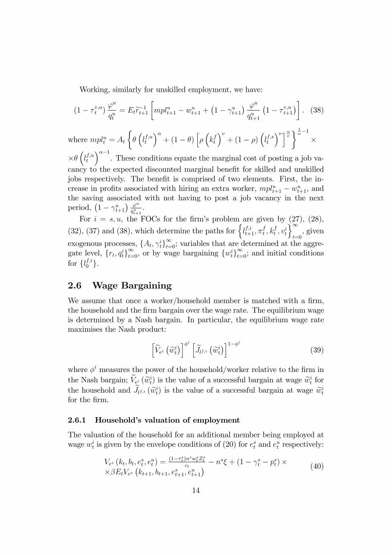
Working, similarly for unskilled employment, we have:

(1� � v;ut )'u

qut= Eter�1t+1 �mplut+1 � wut+1 +

�1� ut+1

� 'u

qut+1

�1� � v;ut+1

��: (38)

where mplut = At

���lf;ut

��+ (1� �)

h��kft

��+ (1� �)

�lf;st

��i��� 1��1

�

���lf;ut

���1. These conditions equate the marginal cost of posting a job va-

cancy to the expected discounted marginal bene�t for skilled and unskilledjobs respectively. The bene�t is comprised of two elements. First, the in-crease in pro�ts associated with hiring an extra worker, mplut+1 � wut+1, andthe saving associated with not having to post a job vacancy in the nextperiod,

�1� ut+1

�'u

qut+1.

For i = s; u, the FOCs for the �rm�s problem are given by (27), (28),

(32), (37) and (38), which determine the paths fornlf;it+1; �

ft ; k

ft ; v

it

o1t=0, given

exogenous processes, fAt; itg1t=0; variables that are determined at the aggre-

gate level, frt; qitg1t=0, or by wage bargaining fwitg

1t=0; and initial conditions

for flf;i0 g.

2.6 Wage Bargaining

We assume that once a worker/household member is matched with a �rm,the household and the �rm bargain over the wage rate. The equilibrium wageis determined by a Nash bargain. In particular, the equilibrium wage ratemaximises the Nash product:heVei � ewit�i�i h eJlf;i � ewit�i1��i (39)

where �i measures the power of the household/worker relative to the �rm inthe Nash bargain; eVei ( ewit) is the value of a successful bargain at wage ewit forthe household and eJlf;i ( ewit) is the value of a successful bargain at wage ewitfor the �rm.

2.6.1 Household�s valuation of employment

The valuation of the household for an additional member being employed atwage wit is given by the envelope conditions of (20) for e

st and e

ut respectively:

Ves (kt; bt; est ; e

ut ) =

(1��st )nswstZstct

� ns� + (1� st � pst)���EtVes

�kt+1; bt+1; e

st+1; e

ut+1

� (40)

14

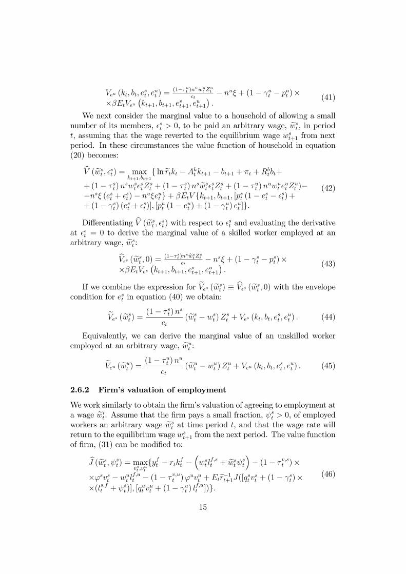
Veu (kt; bt; est ; e

ut ) =

(1��ut )nuwut Zutct

� nu� + (1� ut � put )���EtVeu

�kt+1; bt+1; e

st+1; e

ut+1

�:

(41)

We next consider the marginal value to a household of allowing a smallnumber of its members, �st > 0, to be paid an arbitrary wage, ewst , in periodt, assuming that the wage reverted to the equilibrium wage wst+1 from nextperiod. In these circumstances the value function of household in equation(20) becomes:bV ( ewst ; �st) = max

kt+1;bt+1f ln ertkt � Akt kt+1 � bt+1 + �t +Rb

tbt+

+(1� � st)nswst e

stZ

st + (1� � st)n

s ewst �stZst + (1� �ut )n

uwut eutZ

ut )�

�ns� (est + �st)� nu�eut g+ �EtV fkt+1; bt+1; [pst (1� est � �st)++ (1� st) (e

st + �st)]; [p

ut (1� eut ) + (1� ut ) e

ut ]g:

(42)

Di¤erentiating bV ( ewst ; �st) with respect to �st and evaluating the derivativeat �st = 0 to derive the marginal value of a skilled worker employed at anarbitrary wage, ewst :bV�s ( ewst ; 0) = (1��st )ns ewstZst

ct� ns� + (1� st � pst)�

��EtVes�kt+1; bt+1; e

st+1; e

ut+1

�:

(43)

If we combine the expression for eVes ( ewst ) � bV�s ( ewst ; 0) with the envelopecondition for est in equation (40) we obtain:

eVes ( ewst ) = (1� � st)ns

ct( ewst � wst )Z

st + Ves (kt; bt; e

st ; e

ut ) : (44)

Equivalently, we can derive the marginal value of an unskilled workeremployed at an arbitrary wage, ewut :

eVeu ( ewut ) = (1� �ut )nu

ct( ewut � wut )Z

ut + Veu (kt; bt; e

st ; e

ut ) : (45)

2.6.2 Firm�s valuation of employment

We work similarly to obtain the �rm�s valuation of agreeing to employment ata wage ewit. Assume that the �rm pays a small fraction, st > 0, of employedworkers an arbitrary wage ewst at time period t, and that the wage rate willreturn to the equilibrium wage wst+1 from the next period. The value functionof �rm, (31) can be modi�ed to:

bJ ( ewst ; st) = maxvst ;v

ut

fyft � rtkft �

�wst l

f;st + ewst st�� (1� � v;st )�

�'svst � wut lf;ut � (1� � v;ut )'

uvut + Eter�1t+1J([qst vst + (1� st)��(ls;ft + st)]; [q

ut v

ut + (1� ut ) l

f;ut ])g:

(46)

15

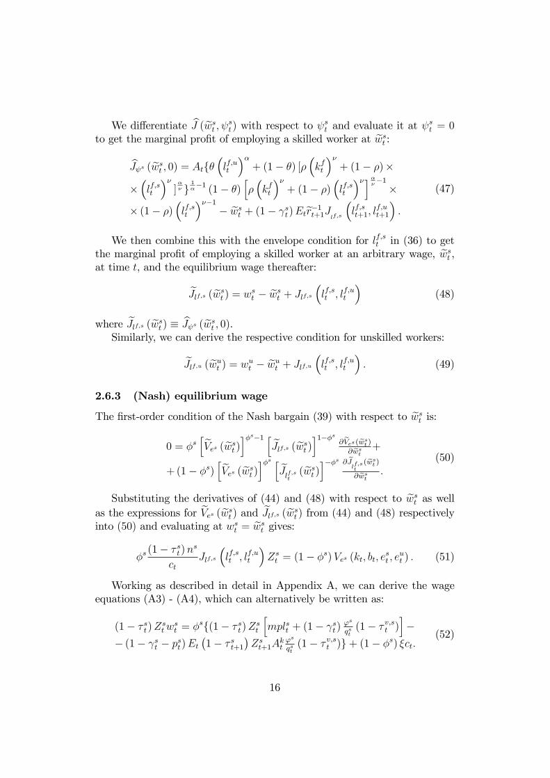
We di¤erentiate bJ ( ewst ; st) with respect to st and evaluate it at st = 0to get the marginal pro�t of employing a skilled worker at ewst :

bJ s ( ewst ; 0) = Atf��lf;ut

��+ (1� �) [�

�kft

��+ (1� �)�

��lf;st

��]�� g

1��1 (1� �)

h��kft

��+ (1� �)

�lf;st

��i���1�� (1� �)

�lf;st

���1� ewst + (1� st)Eter�1t+1Jlf;s �lf;st+1; lf;ut+1� :

(47)

We then combine this with the envelope condition for lf;st in (36) to getthe marginal pro�t of employing a skilled worker at an arbitrary wage, ewst ,at time t, and the equilibrium wage thereafter:

eJlf;s ( ewst ) = wst � ewst + Jlf;s�lf;st ; lf;ut

�(48)

where eJlf;s ( ewst ) � bJ s ( ewst ; 0).Similarly, we can derive the respective condition for unskilled workers:

eJlf;u ( ewut ) = wut � ewut + Jlf;u�lf;st ; lf;ut

�: (49)

2.6.3 (Nash) equilibrium wage

The �rst-order condition of the Nash bargain (39) with respect to ewst is:0 = �s

heVes ( ewst )i�s�1 h eJlf;s ( ewst )i1��s @ eVes ( ewst )@ ewst +

+(1� �s)heVes ( ewst )i�s h eJlf;st ( ewst )i��s @ eJlf;st ( ewst )

@ ewst :(50)

Substituting the derivatives of (44) and (48) with respect to ewst as wellas the expressions for eVes ( ewst ) and eJlf;s ( ewst ) from (44) and (48) respectivelyinto (50) and evaluating at wst = ewst gives:

�s(1� � st)n

s

ctJlf;s

�lf;st ; lf;ut

�Zst = (1� �s)Ves (kt; bt; e

st ; e

ut ) : (51)

Working as described in detail in Appendix A, we can derive the wageequations (A3) - (A4), which can alternatively be written as:

(1� � st)Zstw

st = �sf(1� � st)Z

st

hmplst + (1� st)

's

qst(1� � v;st )

i�

� (1� st � pst)Et�1� � st+1

�Zst+1A

kt's

qst(1� � v;st )g+ (1� �s) �ct:

(52)

16

(1� �ut )Zut w

ut = �uf(1� �ut )Z

ut

hmplut + (1� ut )

'u

qut(1� � v;ut )

i�

� (1� ut � put )Et�1� �ut+1

�Zut+1A

kt'u

qut(1� � v;ut )g+ (1� �u) �ct

(53)

These equations are generalisations of wage equations under Nash bar-gaining obtained in the literature (see e.g. Shimer (2010)). For i = s; u, thereturn of an additional worker to the household is given by (1� � it)Z

itw

it, i.e.

the after-tax e¤ective (or productivity-adjusted) wage. In equilibrium, thisis equal to a weighted average of the e¤ective marginal product of labourunder search and matching, i.e. (1� � it)Z

it

hmplit + (1� it)

'i

qit

�1� � v;it

�i�

(1� it � pit)Et�1� � it+1

�Zit+1A

kt'i

qit

�1� � v;it

�, and the marginal rate of sub-

stitution between consumption and leisure, MRSi, i.e. �ct, with the weightsgiven by the bargaining power of the worker. The MRSi follows the com-mon de�nition of the ratio of the marginal utility of leisure, �, over the mar-ginal utility of consumption, 1=ct. The e¤ective marginal product of labourmeasures the additional after-tax productivity-adjusted output generated bymoving a worker from unemployment to employment. It is comprised of(i) the direct after-tax increase in output provided by an additional skilledworker, mplit; (ii) the additional savings in terms of resources that would berequired to post a vacancy if the matched job survives, (1� it)

'i

qit

�1� � v;it

�,

where (1� it) is the probability that a worker will remain in place in thenext period and 'i

qit

�1� � v;it

�is the cost per job posting multiplied by the

duration that the job needs to be posted, 1qit;7 (iii) the increase in job-posting

costs for the �rm implied by the decrease in future successful matches due tothe increase in employment, (1� it � pit)Et

�1� � it+1

�Zit+1A

kt'i

qit

�1� � v;it

�.

Note that an increase in current employment increases future unemployment(and thus the requirement for the �rm to post a vacancy to �ll the lostjob) by @st+1

@et= (1� it � pit), because there is reduction in the number of

workers who search for jobs. Furthermore, note that these costs need to bediscounted by the price of transferring resources between periods, Akt , whichequals, from (23), expected future returns to investment discounted by thestochastic discount factor.The above wage equations hold when there is no OJL and under purely

external OJL. If we employ the alternative OJL mechanism which inter-nalises own employment on labour productivity, the right hand side of the

7Note that from (37) - (38), 'i

qit

�1� �v;it

�is also equal to the expected bene�t to the

�rm from posting a job.

17

above equations respectively are multiplied by the term:24�i + �1� �i� �Zit + eit

@Zit@eit

�Zit

35�1 ; i = s; u

where @Zst@est

= �ss (est)�s�1 (eut )

1��s ; and @Zut@eut

= (1� �u) u (est)�u (eut ). These

extra terms: (i) collapse to unity under external OJL, i.e. when @Zit@eit

= 0;

(ii) are less than one,8 implying that internalising OJL creates a channelthat tends to reduce the Nash bargained wage, relative to the cases of noor external OJL. When the workers internalise the e¤ect of employment ontheir productivity and thus on their returns, they are willing to work for alower wage rate.

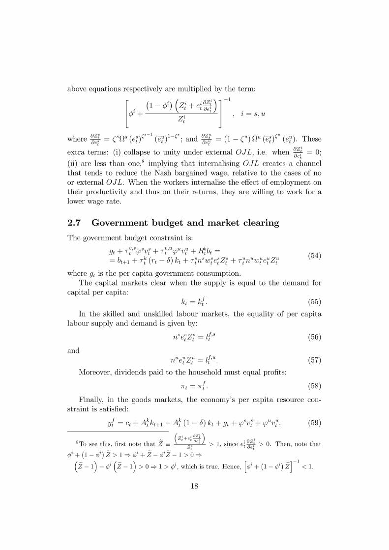
2.7 Government budget and market clearing

The government budget constraint is:

gt + � v;st 'svst + � v;ut 'uvut +Rbtbt =

= bt+1 + � kt (rt � �) kt + � stnswst e

stZ

st + �ut n

uwut eutZ

ut

(54)

where gt is the per-capita government consumption.The capital markets clear when the supply is equal to the demand for

capital per capita:kt = kft : (55)

In the skilled and unskilled labour markets, the equality of per capitalabour supply and demand is given by:

nsestZst = lf;st (56)

andnueutZ

ut = lf;ut : (57)

Moreover, dividends paid to the household must equal pro�ts:

�t = �ft : (58)

Finally, in the goods markets, the economy�s per capita resource con-straint is satis�ed:

yft = ct + Akt kt+1 � Akt (1� �) kt + gt + 'svst + 'uvut : (59)

8To see this, �rst note that eZ �

�Zit+e

it

@Zit@eit

�Zit

> 1, since eit@Zit@eit

> 0. Then, note that

�i +�1� �i

� eZ > 1) �i + eZ � �i eZ � 1 > 0)� eZ � 1�� �i � eZ � 1� > 0) 1 > �i, which is true. Hence,h�i +

�1� �i

� eZi�1 < 1.18

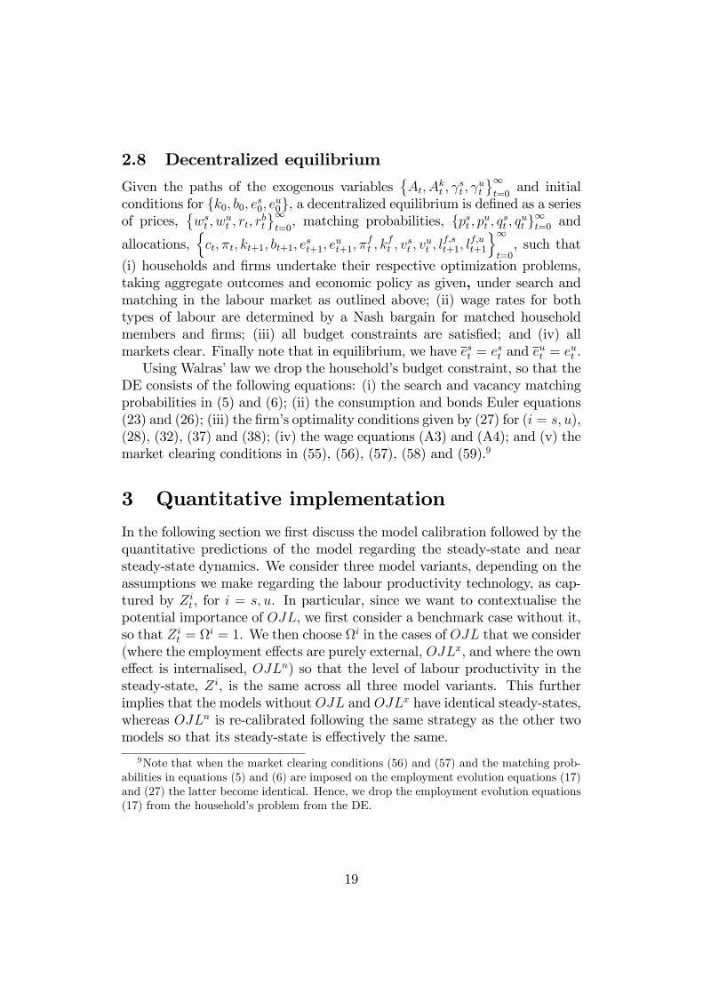
2.8 Decentralized equilibrium

Given the paths of the exogenous variables�At; A

kt ;

st ;

ut

1t=0

and initialconditions for fk0; b0; es0; eu0g, a decentralized equilibrium is de�ned as a seriesof prices,

�wst ; w

ut ; rt; r

bt

1t=0, matching probabilities, fpst ; put ; qst ; qut g

1t=0 and

allocations,nct; �t; kt+1; bt+1; e

st+1; e

ut+1; �

ft ; k

ft ; v

st ; v

ut ; l

f;st+1; l

f;ut+1

o1t=0, such that

(i) households and �rms undertake their respective optimization problems,taking aggregate outcomes and economic policy as given, under search andmatching in the labour market as outlined above; (ii) wage rates for bothtypes of labour are determined by a Nash bargain for matched householdmembers and �rms; (iii) all budget constraints are satis�ed; and (iv) allmarkets clear. Finally note that in equilibrium, we have est = est and e

ut = eut .

Using Walras�law we drop the household�s budget constraint, so that theDE consists of the following equations: (i) the search and vacancy matchingprobabilities in (5) and (6); (ii) the consumption and bonds Euler equations(23) and (26); (iii) the �rm�s optimality conditions given by (27) for (i = s; u),(28), (32), (37) and (38); (iv) the wage equations (A3) and (A4); and (v) themarket clearing conditions in (55), (56), (57), (58) and (59).9

3 Quantitative implementation

In the following section we �rst discuss the model calibration followed by thequantitative predictions of the model regarding the steady-state and nearsteady-state dynamics. We consider three model variants, depending on theassumptions we make regarding the labour productivity technology, as cap-tured by Zi

t , for i = s; u. In particular, since we want to contextualise thepotential importance of OJL, we �rst consider a benchmark case without it,so that Zi

t = i = 1. We then choose i in the cases of OJL that we consider

(where the employment e¤ects are purely external, OJLx, and where the owne¤ect is internalised, OJLn) so that the level of labour productivity in thesteady-state, Zi, is the same across all three model variants. This furtherimplies that the models without OJL and OJLx have identical steady-states,whereas OJLn is re-calibrated following the same strategy as the other twomodels so that its steady-state is e¤ectively the same.

9Note that when the market clearing conditions (56) and (57) and the matching prob-abilities in equations (5) and (6) are imposed on the employment evolution equations (17)and (27) the latter become identical. Hence, we drop the employment evolution equations(17) from the household�s problem from the DE.

19

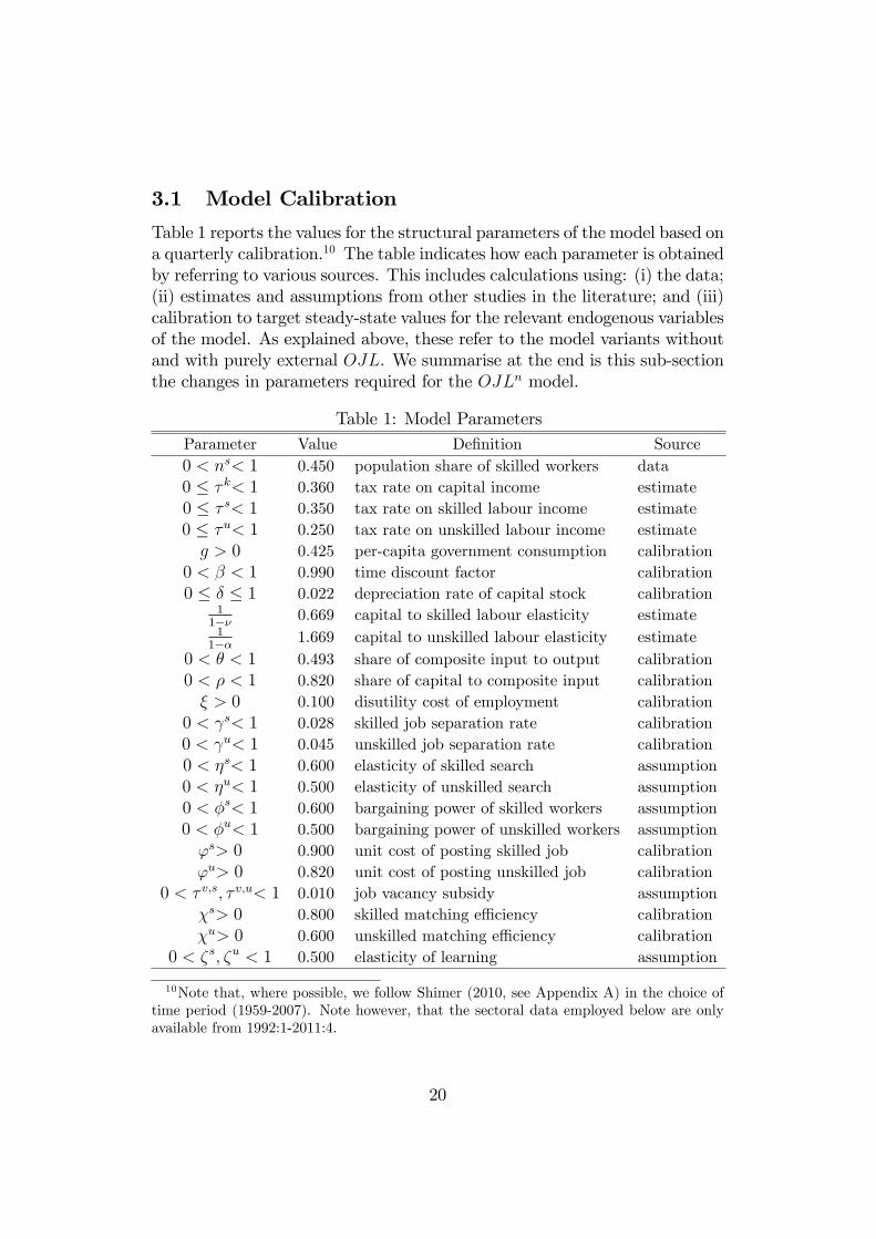
3.1 Model Calibration

Table 1 reports the values for the structural parameters of the model based ona quarterly calibration.10 The table indicates how each parameter is obtainedby referring to various sources. This includes calculations using: (i) the data;(ii) estimates and assumptions from other studies in the literature; and (iii)calibration to target steady-state values for the relevant endogenous variablesof the model. As explained above, these refer to the model variants withoutand with purely external OJL. We summarise at the end is this sub-sectionthe changes in parameters required for the OJLn model.

Table 1: Model ParametersParameter Value De�nition Source0 < ns< 1 0.450 population share of skilled workers data0 � � k< 1 0.360 tax rate on capital income estimate0 � � s< 1 0.350 tax rate on skilled labour income estimate0 � �u< 1 0.250 tax rate on unskilled labour income estimateg > 0 0.425 per-capita government consumption calibration

0 < � < 1 0.990 time discount factor calibration0 � � � 1 0.022 depreciation rate of capital stock calibration

11�� 0.669 capital to skilled labour elasticity estimate1

1�� 1.669 capital to unskilled labour elasticity estimate0 < � < 1 0.493 share of composite input to output calibration0 < � < 1 0.820 share of capital to composite input calibration� > 0 0.100 disutility cost of employment calibration

0 < s< 1 0.028 skilled job separation rate calibration0 < u< 1 0.045 unskilled job separation rate calibration0 < �s< 1 0.600 elasticity of skilled search assumption0 < �u< 1 0.500 elasticity of unskilled search assumption0 < �s< 1 0.600 bargaining power of skilled workers assumption0 < �u< 1 0.500 bargaining power of unskilled workers assumption's> 0 0.900 unit cost of posting skilled job calibration'u> 0 0.820 unit cost of posting unskilled job calibration

0 < � v;s; � v;u< 1 0.010 job vacancy subsidy assumption�s> 0 0.800 skilled matching e¢ ciency calibration�u> 0 0.600 unskilled matching e¢ ciency calibration

0 < �s; �u < 1 0.500 elasticity of learning assumption

10Note that, where possible, we follow Shimer (2010, see Appendix A) in the choice oftime period (1959-2007). Note however, that the sectoral data employed below are onlyavailable from 1992:1-2011:4.

20

3.1.1 Population shares, policy, discount and depreciation rates

We use data from Acemoglu and Autor (2011) for the period (1963-2008)to calculate the population share of skilled workers, ns = 0:45. Consistentwith the range used in the literature, the time discount factor, � = 0:99,is set to give an annual return to capital, net of depreciation, of about 4%.Similarly the depreciation rate, � = 0:022, is calibrated to target a quarterlysteady-state capital to output ratio of about 8 which on an annual basis isconsistent with a ratio of around 2. Following Uhlig (2010) we set the taxrate on capital income to 36%. Moreover, we choose the two labour incometax rates to be � s = 35% and �u = 25%, which imply a weighted averageclose to the 28% labour income tax rate used in Uhlig (2010). The level ofgovernment spending is set so that the debt to output ratio is 0:63 or inquarterly terms 2:52 (as in Uhlig (2010)).

3.1.2 Production

The elasticities of substitution between skilled labour and capital and be-tween unskilled labour and capital have been estimated by Krusell et al.(2000). We use their estimates, so that � = �0:495 and � = 0:401. Toensure the skill premium and labour share in income are consistent with thedata, � and � respectively are calibrated to 0:493 and 0:82 (see, e.g. Lindquist(2004), He and Liu (2008), Pourpourides (2011) and He (2012) who use asimilar approach to calibrating the production function). The target valuefor the skill premium of approximately 1:68 is obtained from Acemoglu andAutor (2011) for the period (1963-2008). We measure the labour incomeshare using data from National Income and Product Accounts Table 1.10,1959-2013, which gives a value of approximately 0.66. Finally, the parame-ters capturing steady-state TFP and investment-speci�c technical change,i.e. A and Ak are normalised to unity.

3.1.3 Utility function and job separation rates

Following Shimer (2010) we set the disutility of employment parameter, � =0:1, to imply an aggregate unemployment rate of about 5%. Also note,that Shimer (2005) reports that an average employment exit probability of0:034. Given this and the assumption that skilled labour has a lower jobseparation rate (see, e.g. Fallick and Fleischman (2004), Hagedorn et al.(2010), and Pilossoph (2012)) we set the job separation rates, s = 0:028and u = 0:045, to approximately match the sectoral unemployment rates of

21

3% and 7% respectively.11

3.1.4 New matches and bargaining power

The values used for the elasticities of new matches with respect to searchtime, �s = 0:6 and �u = 0:5, are within the range of econometric evidencereported in Petrongolo and Pissarides (2001). To ensure that the Hosios(1990) condition is satis�ed we set the relative bargaining power of worker inthe skilled and unskilled sectors respectively to �s = 0:6 and �u = 0:5 (see,Cahuc et al. (2006) who �nd that skilled workers have higher bargainingpower).

3.1.5 Job posting costs and subsidy

Pissarides (1994), Acemoglu (2001) and Krause and Lubik (2006 and 2010)suggest that the �ow cost of posting a vacancy is higher in �good� jobs.Following these studies, we assume that the job posting for skilled is greaterthan that for unskilled labour, i.e. 's > 'u. These parameters are calibratedto ensure aggregate job costs as a share of GDP of about 2.5% which cohereswith Arseneau and Chugh (2012) and aggregate labour market tightness ofabout unity which is the value used in Pissarides (1998) and Campolmi andGnocchi (2014). Also following Campolmi et al. (2011) we set the vacancysubsidy rate to 1%.

3.1.6 Matching e¢ ciency and OJL

Consistent with an aggregate unemployment rate of 5% and an average em-ployment exit probability of 0:034, Shimer (2010, see p. 67) implies a job�nding probability about 0:65. Following this approach for each labour mar-ket gives us target probabilities of ps = 0:828 and put = 0:591 which weobtain by calibrating �s = 0:8 and �u = 0:6. The �nding probabilitiesin turn imply unemployment durations of about 1:21 and 1:69 quarters forskilled and unskilled respectively. The calibration also suggests that the job�lling rate is higher for the skilled versus the unskilled consistent with Krauseand Lubik (2006 and 2010). As explained above, we present the models re-sults below both without and with learning. In the former, Zs

t = Zut = 1

in (10-11). In both forms of latter (i.e. OJLx and OJLn) we set the ex-ponents �s = �u = 0:5 and calibrate s and u so that in the steady-state

11The sectoral employment and unemployment data are from the monthly Labor ForceStatistics, Current Population Survey for period (1992:1-2011:4). It reports data for civil-ian non-institutional population 25 years and over by educational attainment. Skilledworkers are those with a Bachelor�s degree and higher.

22

the Z functions are equal to unity as under no learning. This requires thats = u = 1:055.12

3.2 Steady-state

The steady-state implied by the above calibration is reported in Table 2 forthe models without and with purely external learning. These results showthat great ratios are well in line with the U.S. data. Moreover, the remainingvalues cohere with the targets discussed in the calibration above. For thethird model variant, the results are quantitatively similar. To ensure thatthe model under OJLn implies an analogous steady-state with the remainingtwo model-variants, we re-calibrate � = 0:500, 's = 1:600, 'u = 1:520, andg = 0:401, following the same calibration strategy outlined above. Note thatas discussed in Section 2.6.3, when workers internalise OJL, bargained wagestend to be lower and thus unemployment lower. Therefore, to maintain thesame level of unemployment and labour market tightness in the steady-state,job-posting costs need to increase.

Table 2: Steady-statecy

ky

gy

by

wey

vy

ss su s

0.571 8.198 0.225 2.520 0.660 0.024 0.033 0.071 0.054ws

wuer rb zs zu ps pu qs qu

1.680 0.010 0.010 1.089 0.971 0.828 0.591 0.760 0.609

3.3 Stochastic processes

When undertaking the model simulations we draw the four processes dis-cussed above from a multivariate normal distribution, denoted x = N (x;�; )where x = ["At ; "

Ak

t ; "gs

t ; "gu

t ]; x is the vector of means and � is the variance-covariance matrix of shocks. The parameters of stochastic processes drivingthe model are reported in Table 3. The autocorrelation parameter of TFPis set equal to 0.95, following Gertler and Trigari (2009), and Arseneau andChugh (2012). As in the literature, the volatility parameter, �A, is cal-ibrated to match the standard deviation of HP-�ltered output, 0.011. Re-

12Given the lack of data for exponents in the learning functions, we experiment withsome alternative combinations. For example, we place more weight on the own-elasticityfor the skilled, i.e. �s = 0:8 and (1 � �s) = 0:2 while at the same time keeping weight ofthe own-elasticity for the unskilled: (i) the same, �u = 0:5 and (1� �u) = 0:5; (ii) higher,�u = 0:8 and (1� �u) = 0:2; and (iii) lower, �u = 0:2 and (1� �u) = 0:8. We �nd that theresults reported below, including steady-state, second-moments, impulse responses and�scal multipliers, are robust these to alternative parameterisations. This applies to boththe OJLx and OJLn setups.

23

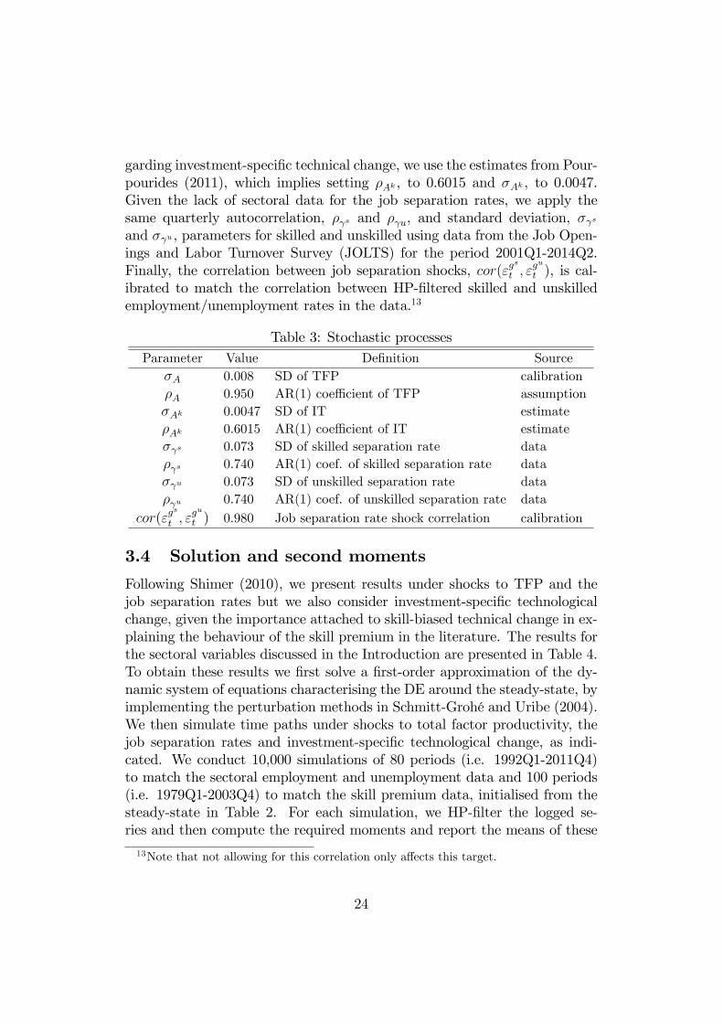
garding investment-speci�c technical change, we use the estimates from Pour-pourides (2011), which implies setting �Ak , to 0.6015 and �Ak , to 0.0047.Given the lack of sectoral data for the job separation rates, we apply thesame quarterly autocorrelation, � s and � u, and standard deviation, � sand � u , parameters for skilled and unskilled using data from the Job Open-ings and Labor Turnover Survey (JOLTS) for the period 2001Q1-2014Q2.Finally, the correlation between job separation shocks, cor("g

s

t ; "gu

t ), is cal-ibrated to match the correlation between HP-�ltered skilled and unskilledemployment/unemployment rates in the data.13

Table 3: Stochastic processesParameter Value De�nition Source

�A 0.008 SD of TFP calibration�A 0.950 AR(1) coe¢ cient of TFP assumption�Ak 0.0047 SD of IT estimate�Ak 0.6015 AR(1) coe¢ cient of IT estimate� s 0.073 SD of skilled separation rate data� s 0.740 AR(1) coef. of skilled separation rate data� u 0.073 SD of unskilled separation rate data� u 0.740 AR(1) coef. of unskilled separation rate data

cor("gs

t ; "gu

t ) 0.980 Job separation rate shock correlation calibration

3.4 Solution and second moments

Following Shimer (2010), we present results under shocks to TFP and thejob separation rates but we also consider investment-speci�c technologicalchange, given the importance attached to skill-biased technical change in ex-plaining the behaviour of the skill premium in the literature. The results forthe sectoral variables discussed in the Introduction are presented in Table 4.To obtain these results we �rst solve a �rst-order approximation of the dy-namic system of equations characterising the DE around the steady-state, byimplementing the perturbation methods in Schmitt-Grohé and Uribe (2004).We then simulate time paths under shocks to total factor productivity, thejob separation rates and investment-speci�c technological change, as indi-cated. We conduct 10,000 simulations of 80 periods (i.e. 1992Q1-2011Q4)to match the sectoral employment and unemployment data and 100 periods(i.e. 1979Q1-2003Q4) to match the skill premium data, initialised from thesteady-state in Table 2. For each simulation, we HP-�lter the logged se-ries and then compute the required moments and report the means of these

13Note that not allowing for this correlation only a¤ects this target.

24

moments across the simulations in Table 4.

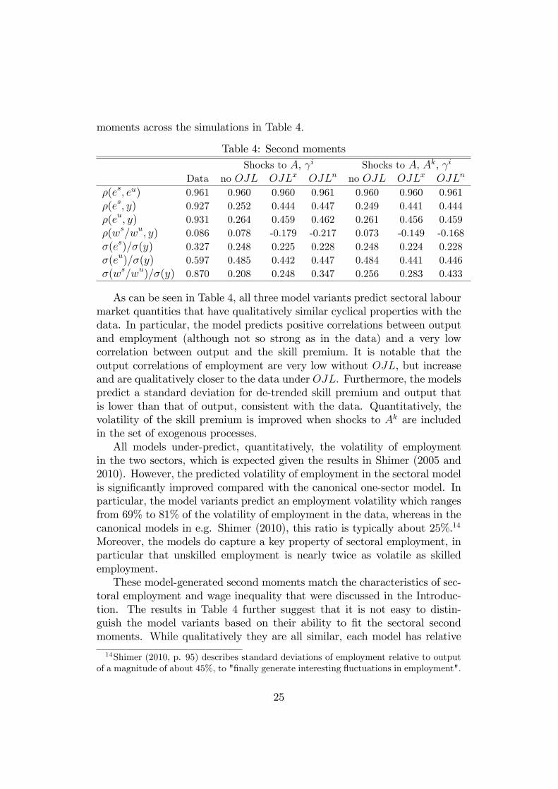
Table 4: Second momentsShocks to A, i Shocks to A, Ak, i

Data no OJL OJLx OJLn no OJL OJLx OJLn

�(es; eu) 0.961 0.960 0.960 0.961 0.960 0.960 0.961�(es; y) 0.927 0.252 0.444 0.447 0.249 0.441 0.444�(eu; y) 0.931 0.264 0.459 0.462 0.261 0.456 0.459�(ws=wu; y) 0.086 0.078 -0.179 -0.217 0.073 -0.149 -0.168�(es)=�(y) 0.327 0.248 0.225 0.228 0.248 0.224 0.228�(eu)=�(y) 0.597 0.485 0.442 0.447 0.484 0.441 0.446�(ws=wu)=�(y) 0.870 0.208 0.248 0.347 0.256 0.283 0.433

As can be seen in Table 4, all three model variants predict sectoral labourmarket quantities that have qualitatively similar cyclical properties with thedata. In particular, the model predicts positive correlations between outputand employment (although not so strong as in the data) and a very lowcorrelation between output and the skill premium. It is notable that theoutput correlations of employment are very low without OJL, but increaseand are qualitatively closer to the data under OJL. Furthermore, the modelspredict a standard deviation for de-trended skill premium and output thatis lower than that of output, consistent with the data. Quantitatively, thevolatility of the skill premium is improved when shocks to Ak are includedin the set of exogenous processes.All models under-predict, quantitatively, the volatility of employment

in the two sectors, which is expected given the results in Shimer (2005 and2010). However, the predicted volatility of employment in the sectoral modelis signi�cantly improved compared with the canonical one-sector model. Inparticular, the model variants predict an employment volatility which rangesfrom 69% to 81% of the volatility of employment in the data, whereas in thecanonical models in e.g. Shimer (2010), this ratio is typically about 25%.14

Moreover, the models do capture a key property of sectoral employment, inparticular that unskilled employment is nearly twice as volatile as skilledemployment.These model-generated second moments match the characteristics of sec-

toral employment and wage inequality that were discussed in the Introduc-tion. The results in Table 4 further suggest that it is not easy to distin-guish the model variants based on their ability to �t the sectoral secondmoments. While qualitatively they are all similar, each model has relative

14Shimer (2010, p. 95) describes standard deviations of employment relative to outputof a magnitude of about 45%, to "�nally generate interesting �uctuations in employment".

25

successes compared with the others. However, the models with OJL areclearly preferable to the model that does not allow for OJL regarding theoutput correlations for employment. Therefore, to analyse the e¤ect of pol-icy below we present results for all three model variants. This allows us toprovide a range for the likely size of the �scal multipliers arising from tar-geted labour market interventions and thus to quantitatively evaluate theimportance of OJL or skill erosion for the e¤ects of policy interventions.

4 Fiscal interventions in the labour market

We next consider the e¤ect of targeted labour market policies in the formof job-posting subsidies and income tax cuts.15 In particular, we focus thefollowing policy experiments. First, that the government increases � v;st tem-porarily by one percentage point and lets government debt absorb the �scalimplications of the shock. Second, we examine the e¤ects of a similar in-crease in � v;st under �xed government debt, so that the policy interventionis �nanced by a proportional increase in the labour and capital income taxrates.16 This budgetary restriction is particularly relevant given the current,post �nancial crisis economic reality that severely limits the use of debt to�nance �scal interventions in most advanced economies. We then repeat thesame experiments for an increase in � v;ut by one percentage point. Finally, wediscuss the implications of labour market interventions in the form of cuts inthe labour income taxes by one-percentage point.17 To implement the aboveexperiments, we assume that when temporarily shocked, vacancy subsidiesand income taxes follow standard AR(1) processes.18

We �rst discuss the impulse responses of the �rst policy experiment indetail, to analyse the channels via which vacancy subsidies a¤ect employmentin the two sectors and output. We focus on the two models that have thesame calibration and steady-state, i.e. without OJL and under OJLx, since

15See Campolimi et al. (2011) and Faia et al. (2013) who conduct similar analysis inthe context of a search and matching model with endogenous participation and a labourselection model with turnover costs and Nash bargained wages, respectively.16In this case, we �x the level of government debt to its steady-state level, let one of the

income taxes to be the residual policy instrument in the government budget constraint,and �x the remaining two income taxes to remain in the same proportion with the residualincome tax as in the steady-state.17Note that normalising the tax cuts to have the same �scal implications as the vacancy

subsidy interventions yields e¤ectively the same results.18Following Campolmi et al. (2011) we set the AR(1) parameters for the vacancy subsi-

dies to 0.90 and following Angelopoulos et al. we set the AR(1) parameters on the skilledand unskilled income taxes to 0.950 and 0.920.

26

the e¤ects are directly comparable, and thus we can trace the workings ofthe OJL mechanism following the policy intervention. We then summarisethe implications for output and unemployment in each case by calculatingthe �scal multipliers for the remaining labour market interventions that weconsider. Following Leeper et al. (2009) we calculate �scal multipliers asfollows:

FMk =

kPj=0

�jQi=0

R�1t+i

��yt+j

kPj=0

�jQi=0

R�1t+i

��xt+j

(60)

where Rt � 1 + (1� � kt )(rt � �); �yt = (yt � y) and �xt = (xt � x). For thevacancy subsidy multipliers�xt = e� v;it �e� v;i, where i = s; u and e� v;it = 'ivit�

v;it

gives the cost of the subsidy. Finally for the tax multipliers �xt = e� it � e� i,where e� it = ni� itw

iteit (without OJL) and e� it = ni� itw

iteitZ

it (under OJL

x andOJLn) represent the respective costs of the tax reduction.

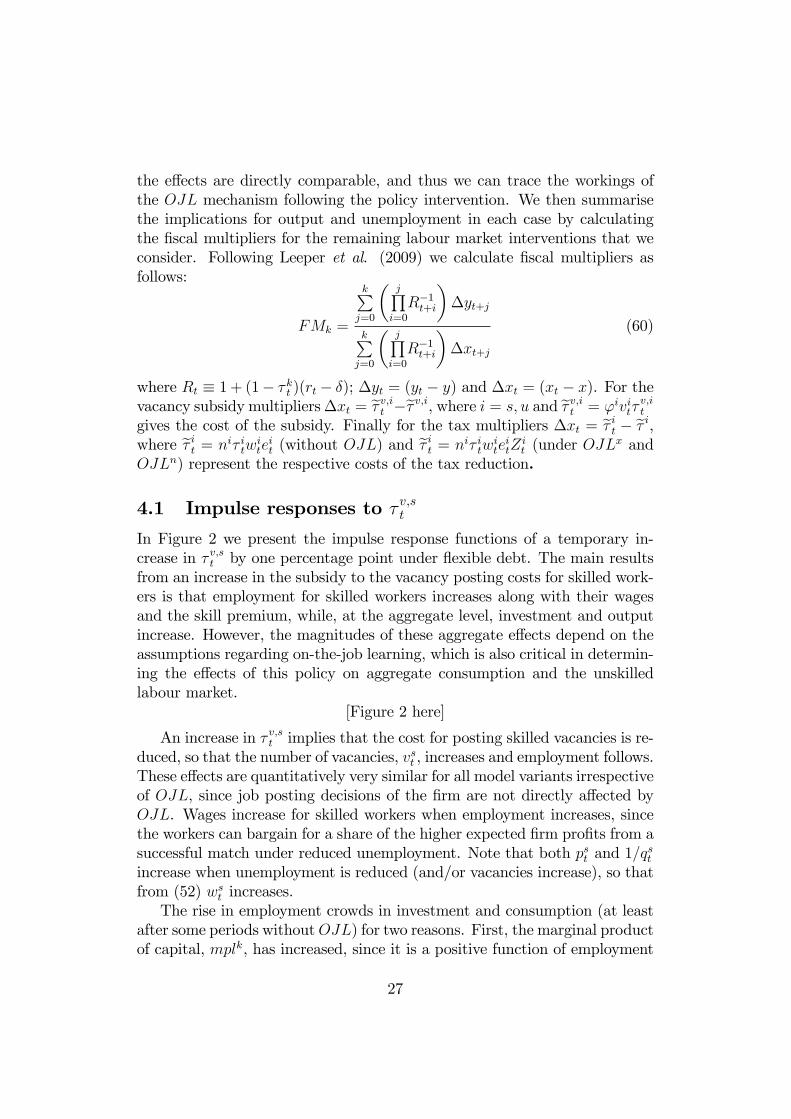
4.1 Impulse responses to � v;stIn Figure 2 we present the impulse response functions of a temporary in-crease in � v;st by one percentage point under �exible debt. The main resultsfrom an increase in the subsidy to the vacancy posting costs for skilled work-ers is that employment for skilled workers increases along with their wagesand the skill premium, while, at the aggregate level, investment and outputincrease. However, the magnitudes of these aggregate e¤ects depend on theassumptions regarding on-the-job learning, which is also critical in determin-ing the e¤ects of this policy on aggregate consumption and the unskilledlabour market.

[Figure 2 here]

An increase in � v;st implies that the cost for posting skilled vacancies is re-duced, so that the number of vacancies, vst , increases and employment follows.These e¤ects are quantitatively very similar for all model variants irrespectiveof OJL, since job posting decisions of the �rm are not directly a¤ected byOJL. Wages increase for skilled workers when employment increases, sincethe workers can bargain for a share of the higher expected �rm pro�ts from asuccessful match under reduced unemployment. Note that both pst and 1=q

st

increase when unemployment is reduced (and/or vacancies increase), so thatfrom (52) wst increases.The rise in employment crowds in investment and consumption (at least

after some periods withoutOJL) for two reasons. First, the marginal productof capital, mplk, has increased, since it is a positive function of employment

27

and this tends to increase investment. Second, the income of the householdhas increased, because of higher employment and wages of skilled, as wellas higher pro�ts of the �rm. In turn, the increased employment and capitalincrease output. Under OJL, consumption, investment and output increaseby more, because the rise in employment has a direct productivity e¤ect onproduction (and thus the marginal product of capital, output, and householdincome). Without OJL, the household income gains are not strong enoughinitially to allow the household to increase both consumption and invest-ment, so that it is optimal to reduce consumption to increase investmenttemporarily.Increases in skilled job posting vacancies also have an e¤ect on the un-

skilled labour market. The increase in est increases the marginal productof unskilled labour, mplu, which tends to increase labour demand and va-cancy postings for unskilled jobs. However, under OJL, there are additionale¤ects. In particular, since est increases the e¤ective quantity of unskilledlabour (by increasing Zu

t ), this tends to decrease mplu, which is decreasing

in the e¤ective quantity of unskilled labour. Therefore, under OJL, there isa channel that tends to mediate the positive e¤ects of � v;st on the unskilledlabour market, so that the �nal e¤ect of � v;st on eut is bigger without OJL.The unskilled wage increases because mplu has risen. Relative to the e¤ectsof � v;st on wst , the positive e¤ects of �

v;st on wut are second order and thus w

ut

rises by less, so that the skill premium increases.

4.2 Fiscal multipliers

We next present and discuss the �scal multipliers for the di¤erent �scal in-terventions in the labour markets.

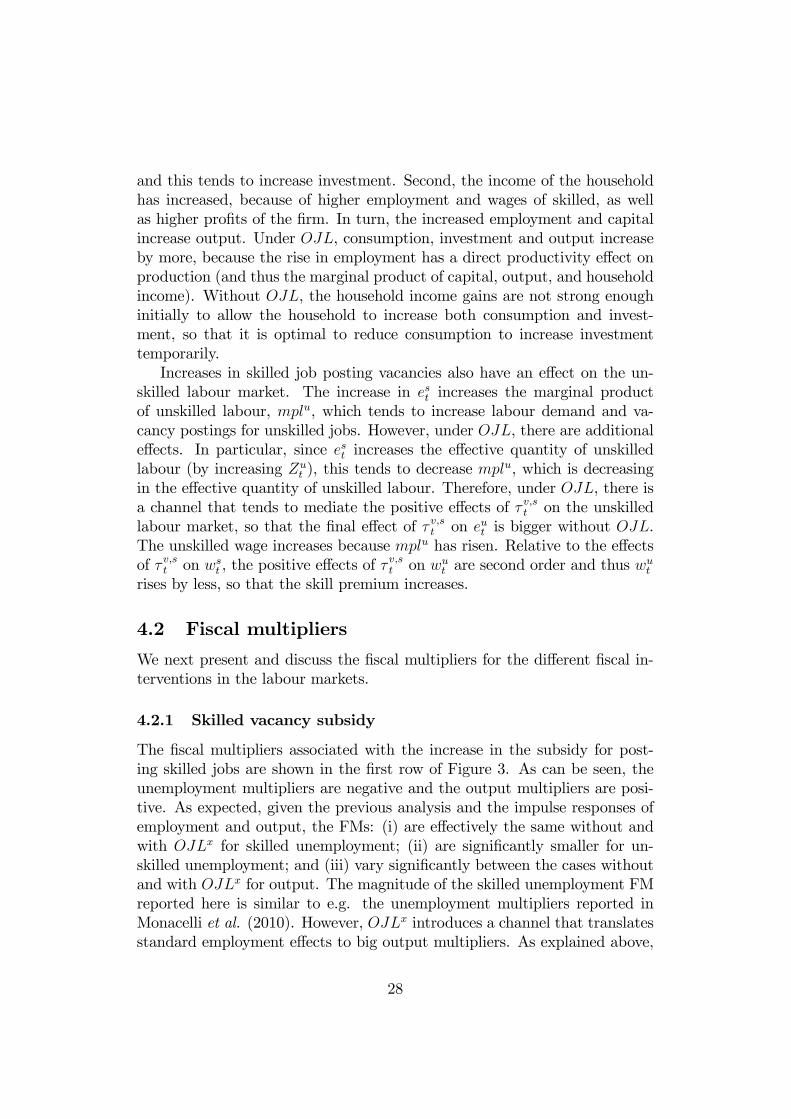
4.2.1 Skilled vacancy subsidy

The �scal multipliers associated with the increase in the subsidy for post-ing skilled jobs are shown in the �rst row of Figure 3. As can be seen, theunemployment multipliers are negative and the output multipliers are posi-tive. As expected, given the previous analysis and the impulse responses ofemployment and output, the FMs: (i) are e¤ectively the same without andwith OJLx for skilled unemployment; (ii) are signi�cantly smaller for un-skilled unemployment; and (iii) vary signi�cantly between the cases withoutand with OJLx for output. The magnitude of the skilled unemployment FMreported here is similar to e.g. the unemployment multipliers reported inMonacelli et al. (2010). However, OJLx introduces a channel that translatesstandard employment e¤ects to big output multipliers. As explained above,

28

in this case the increase in employment crowds in signi�cant investment, asthe increase in labour productivity raises the marginal product of capital, aswell as household income, to high levels. In fact, under OJLx the outputmultiplier is greater than one.

[Figure 3 here]

We then repeat the policy intervention of the increase in the subsidy forposting skilled jobs, this time working with the �xed debt restriction, so thatthe �scal implications of the increased expenditure are met by increases inincome taxation. The �scal multipliers in this case are reported in the secondrow on Figure 3. As can be seen, the size of the multipliers is e¤ectively unaf-fected, suggesting that this type of labour market intervention is potentiallyvery useful in an environment where the ability of the government to usepublic debt to boost the economy is restricted. Since the �scal implicationsof the vacancy subsidy are relatively small, the size of the multipliers is pre-dominantly driven by the change in the target quantities in the numeratorsof (60), for which the e¤ect of the vacancy subsidy is direct and dominatesthe side-e¤ects arising from modest increases in income taxation.

4.2.2 Unskilled vacancy subsidy

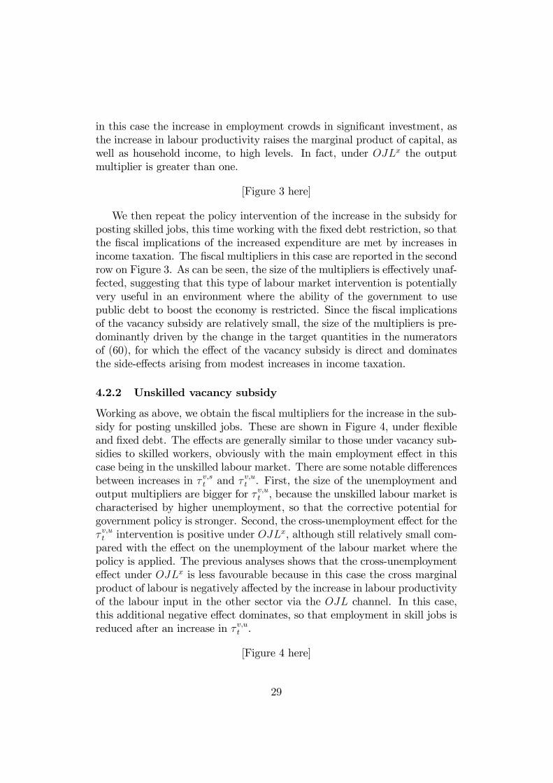
Working as above, we obtain the �scal multipliers for the increase in the sub-sidy for posting unskilled jobs. These are shown in Figure 4, under �exibleand �xed debt. The e¤ects are generally similar to those under vacancy sub-sidies to skilled workers, obviously with the main employment e¤ect in thiscase being in the unskilled labour market. There are some notable di¤erencesbetween increases in � v;st and � v;ut . First, the size of the unemployment andoutput multipliers are bigger for � v;ut , because the unskilled labour market ischaracterised by higher unemployment, so that the corrective potential forgovernment policy is stronger. Second, the cross-unemployment e¤ect for the� v;ut intervention is positive under OJLx, although still relatively small com-pared with the e¤ect on the unemployment of the labour market where thepolicy is applied. The previous analyses shows that the cross-unemploymente¤ect under OJLx is less favourable because in this case the cross marginalproduct of labour is negatively a¤ected by the increase in labour productivityof the labour input in the other sector via the OJL channel. In this case,this additional negative e¤ect dominates, so that employment in skill jobs isreduced after an increase in � v;ut .

[Figure 4 here]

29

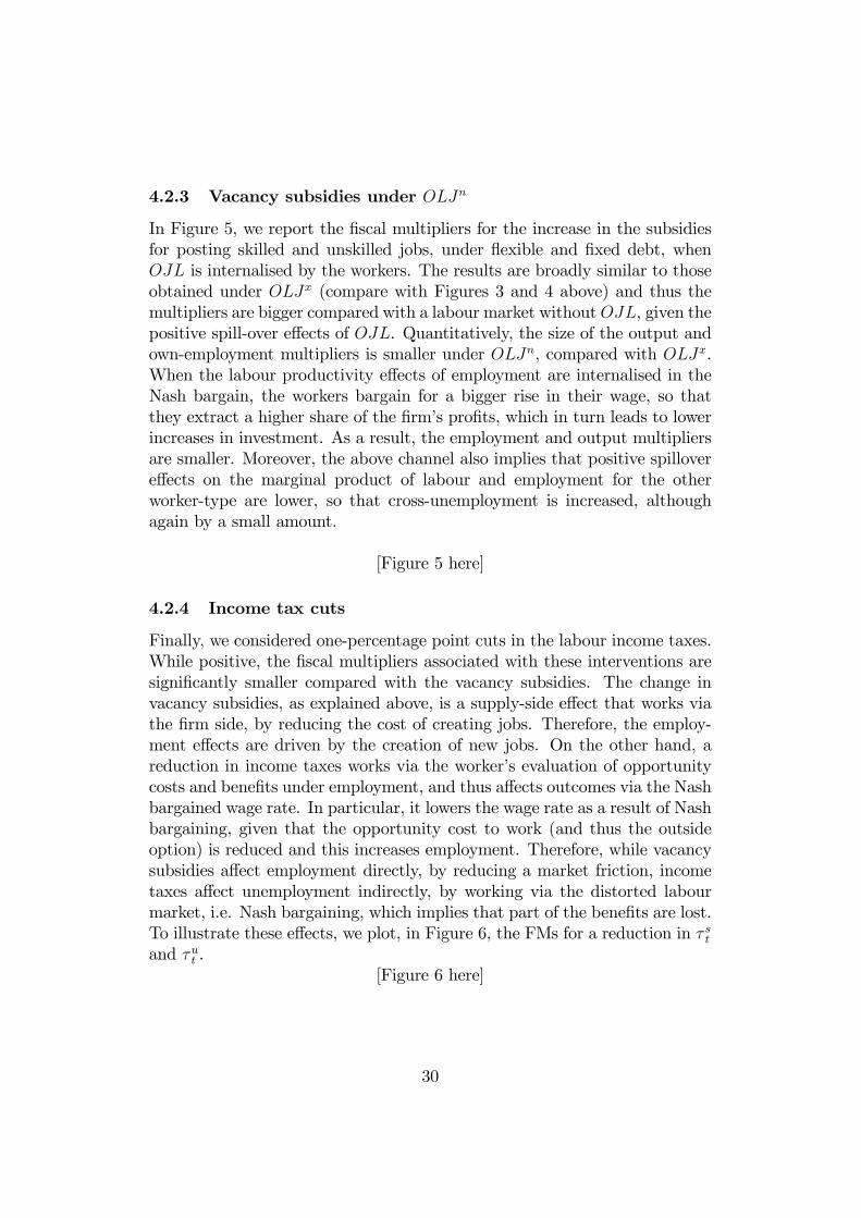
4.2.3 Vacancy subsidies under OLJn

In Figure 5, we report the �scal multipliers for the increase in the subsidiesfor posting skilled and unskilled jobs, under �exible and �xed debt, whenOJL is internalised by the workers. The results are broadly similar to thoseobtained under OLJx (compare with Figures 3 and 4 above) and thus themultipliers are bigger compared with a labour market withoutOJL, given thepositive spill-over e¤ects of OJL. Quantitatively, the size of the output andown-employment multipliers is smaller under OLJn, compared with OLJx.When the labour productivity e¤ects of employment are internalised in theNash bargain, the workers bargain for a bigger rise in their wage, so thatthey extract a higher share of the �rm�s pro�ts, which in turn leads to lowerincreases in investment. As a result, the employment and output multipliersare smaller. Moreover, the above channel also implies that positive spillovere¤ects on the marginal product of labour and employment for the otherworker-type are lower, so that cross-unemployment is increased, althoughagain by a small amount.

[Figure 5 here]

4.2.4 Income tax cuts

Finally, we considered one-percentage point cuts in the labour income taxes.While positive, the �scal multipliers associated with these interventions aresigni�cantly smaller compared with the vacancy subsidies. The change invacancy subsidies, as explained above, is a supply-side e¤ect that works viathe �rm side, by reducing the cost of creating jobs. Therefore, the employ-ment e¤ects are driven by the creation of new jobs. On the other hand, areduction in income taxes works via the worker�s evaluation of opportunitycosts and bene�ts under employment, and thus a¤ects outcomes via the Nashbargained wage rate. In particular, it lowers the wage rate as a result of Nashbargaining, given that the opportunity cost to work (and thus the outsideoption) is reduced and this increases employment. Therefore, while vacancysubsidies a¤ect employment directly, by reducing a market friction, incometaxes a¤ect unemployment indirectly, by working via the distorted labourmarket, i.e. Nash bargaining, which implies that part of the bene�ts are lost.To illustrate these e¤ects, we plot, in Figure 6, the FMs for a reduction in � stand �ut .

[Figure 6 here]

30

5 Conclusions

This paper evaluated the e¤ects of policy interventions on sectoral labourmarkets and the aggregate economy in a business cycle model with search andmatching frictions. We extended the canonical model by including capital-skill complementarity in production, skilled and unskilled labour markets andon-the-job-learning (OJL) within and across skill types. Our policy analysisevaluated the e¤ects of temporary interventions in the labour markets and theaggregate economy. We found �scal multipliers on output from the subsidesto skilled and unskilled vacancies, which were greater than unity when OJLwas external and near unity when it was internal. These large multiplierswere determined by the crowding-in of private investment, which followed theincreases in employment and labour productivity. Without OJL, the labourproductivity channel was absent and caused the output multipliers to fall toabout 0.6. In contrast to the vacancy subsidies, the positive output e¤ectsfrom cutting skilled and unskilled income taxes were near zero,irrespectiveof the presence, or model, of OJL. We �nally found that the e¤ects of thetwo vacancy subsidies did not depend on whether debt or distorting taxeswere used to �nance them. This is particularly good news, and suggests thatthis type of intervention may be useful under the debt restrictions that manygovernments now face in the wake of the �nancial crisis.

References

[1] Acemoglu, D. (2001). �Good jobs versus bad jobs�, Journal of LaborEconomics, 19, 1�21.

[2] Acemoglu, D. and D. Autor (2011). �Skills, tasks and technologies: im-plications for employment and earnings�, in O. Ashenfelter and D. Card(eds.), Handbook of Labor Economics, 4b, 1043-1171, Amsterdam: Else-vier.

[3] Angelopoulos, K., Asimakopoulos, S. and J. Malley (2013). �The optimaldistribution of the tax burden over the business cycle�, CESifo WorkingPaper Series 4468, CESifo Group Munich.

[4] Arseneau, D. and S. Chugh (2012). �Tax smoothing in frictional labormarkets�, Journal of Political Economy, 120, 926-985.

[5] Barro, R. and X. Sala-i-Martin (1994). �Quality improvements in modelsof growth�, CEPR Discussion Papers 1076.

31

[6] Blanchard, O. and P. Diamond (1989). �The beveridge curve�, BrookingsPapers on Economic Activity, 1, 1-60.

[7] Cahuc, P., Postel-Vinay, F. and J. Robin (2006). �Wage bargaining withon-the-job search: theory and evidence�, Econometrica, 74, 323-364.

[8] Campolmi, A. and S. Gnocchi (2014). �Labor market participation, un-employment and monetary Policy�, Bank of Canada working paper,2014-09.

[9] Campolmi A., Faia, E. and R. Winkler (2011). �Fiscal Calculus and theLabor Market�, The B.E. Journal of Macroeconomics, 11, 1-27.

[10] Castro, R. and D. Coen-Pirani (2008). �Why have aggregate skilled hoursbecome so cyclical since the mid-1980s?�, International Economic Re-view, 49, 135-184.

[11] Davis, S. and T. von Wachter (2011). �Recessions and the costs of jobloss�, Brookings Papers on Economic Activity, 43, 1-72.

[12] Dolado, J., Jansen, M. and J. Jimeno (2009). �On-the-job search in amatching model with heterogeneous jobs and workers�, Economic Jour-nal, 119, 200-228.

[13] Doppelt, R. (2014). �Skill �ows: a theory of human capital and unem-ployment�, working paper.

[14] Faia, E., Lechthaler, W. and C. Merkl (2013). �Fiscal stimulus and labormarket policies in Europe�, Journal of Economic Dynamics and Control,37, 483�499

[15] Fallick, B. and C. Fleischman (2004). �Employer-to-employer �ows in theU.S. labor market: the complete picture of gross worker �ows�, WorkingPaper 2004-34, Federal Reserve Board of Governors.

[16] Gertler, M. and A. Trigari (2009). �Unemployment �uctuations withstaggered Nash wage bargaining�, Journal of Political Economy, 117,38-86.

[17] Goldin, C. and L. Katz (2008). The race between education and technol-ogy, Harvard University Press.

[18] Greenwood, J., Hercowitz, Z. and P. Krusell (2000). �The role ofinvestment-speci�c technological change in the business cycle�, EuropeanEconomic Review, 44, 91-115.

32

[19] Hagedorn, M., Manovskii, I. and S. Stetsenko (2010). �Taxation and un-employment in models with heterogeneous workers�, mimeo, Universityof Pennsylvania.

[20] He, H. and Z. Liu (2008). �Investment-speci�c technological change, skillaccumulation, and wage inequality�, Review of Economic Dynamics, 11,314-334.

[21] He, H. (2012). �What Drives the Skill Premium: Technological changeor demographic variation?�, European Economic Review, 56, 1546-1572.

[22] Hosios, A. (1990). �On the e¢ ciency of matching and related models ofsearch and unemployment�, Review of Economic Studies, 57, 279-298.

[23] Katz, L. and K. Murphy (1992). �Changes in relative wages, 1963-1987:supply and demand factors�, The Quarterly Journal of Economics, 107,35-78.

[24] Krause, M. and T. Lubik (2006). �The cyclical upgrading of labour andon-the-job search�, Labour Economics, 13, 459-77.

[25] Krause, M. and T. Lubik (2010). �On-the-job search and the cyclical dy-namics of the labor market�, Federal Reserve Bank of RichmondWorkingPaper Series WP, 10�12.

[26] Krusell, P., Ohanian, L., RÌos-Rull J. and G. Violante (2000). �Capital-skill complementarity and inequality: a macroeconomic analysis�,Econometrica, 68, 1029-1053.

[27] Laureys, L. (2014). �The cost of human capital depreciation during un-employment�, Bank of England Working Paper, No. 505.

[28] Leeper, E., Plante, M., and N. Traum (2010). �Dynamics of �scal �nanc-ing in the United States�, Journal of Econometrics, 156, 304-321.

[29] Lindquist, M. (2004). �Capital�skill complementarity and inequality overthe business cycle�, Review of Economic Dynamics, 7, 519-540.

[30] Merz, M. (1995). �Search in the labor market and the real business cycle�,Journal of Monetary Economics, 36, 269-300.

[31] Monacelli, T., Perotti, R. and A. Trigari (2010). �Unemployment �scalmultipliers�, Journal of Monetary Economics, 57, 531-553.

33

[32] Petrongolo, B. and C. Pissarides (2001). �Looking into the black box: asurvey of the matching function�, Journal of Economic Literature, 39,390-431.

[33] Pilossoph, L. (2012). A multisector equilibrium search model of laborreallocation, Ph.D. thesis, The University of Chicago.

[34] Pissarides, C. (1986). �Vacancies and unemployment in Britain�, Eco-nomic Policy, 3, 499-559.

[35] Pissarides, C. (1994). �Search unemployment with on the job search�,Review of Economic Studies 61, 457�476.

[36] Pissarides, C. (1998). �The impact of employment tax cuts on unemploy-ment and wages: the role of unemployment bene�ts and tax structure�,European Economic Review, 42, 155-183.

[37] Pollak, R. (2013). �Allocating household time: when does e¢ ciency im-ply specialization?�NBER Working Papers 19178.

[38] Pourpourides, P. (2011). �Implicit contracts and the cyclicality of theskill-premium�, Journal of Economic Dynamics and Control, 35, 963-979.

[39] Rogerson, R. and R. Shimer (2011). �Search in macroeconomic modelsof the labor market�, Handbook of Labor Economics, Elsevier.

[40] Romer, P. (1996). �Increasing returns and long-run growth�, Journal ofPolitical Economy, 94, 1002-1037.

[41] Schmitt-Grohe, S. and M. Uribe (2004). �Solving dynamic general equi-librium models using a second-order approximation to the policy func-tion�, Journal of Economic Dynamics and Control, 28, 755-775.

[42] Shimer, R. (2005). �The cyclical behavior of equilibrium unemploymentand vacancies�, American Economic Review, 95, 25�49.

[43] Shimer, R. (2010). Labor Markets and Business Cycles, CREI Lecturesin Macroeconomics, Princeton University Press.

[44] Uhlig, H. (2010). �Some �scal calculus�, American Economic Review,100, 30-34.

34

Appendix A: Derivation of Wage Equations

Using (51) and its one-period lead to eliminate Ves (kt; est ; eut ) and Ves(kt+1;

est+1; eut+1) in the envelope condition for skilled employment (40) yields an

expression whose both sides are multiplied by ct (1� �s) and divided by ns

to give:

�s (1� � st) Jlf;s�lf;st ; lf;ut

�Zst = (1� � st)w

stZ

st (1� �s)�

� (1� �s) ct + (1� st � pst) �Et�s (1��st+1)ct

ct+1�

�Jlf;s�lf;st+1; l

f;ut+1

�Zst+1.

(A1)

Multiplying Et ctct+1

by ert+1ert+1 in (A1), substituting for er�1t+1Jlf;s �lf;st+1; lf;ut+1�using (35) and Jlf;s

�lf;st ; lf;ut

�using (36), and substituting Akt

ctfor �Et

�ert+1ct+1

�in (A1) using the Euler (23) yields:

�shmplst � wst + (1� st)

's

qst(1� � v;st )

i= wst (1� �s)� �(1��s)ct

(1��st )Zst+

+(1� st � pst)Et�s (1��st+1)(1��st )

h's

qst(1� � v;st )

iZst+1Zst

Akt .(A2)

Simplifying the resulting expression gives the Nash wage rate for skilledworkers:

wst = �sfmplst + [1� st � (1� st � pst)� (A3)

�EtAkt

Zst+1

�1� � st+1

�Zst (1� � st)

!]'s

qst(1� � v;st )g+

� (1� �s) ct(1� � st)Z

st

:

Working similarly, we can derive the Nash wage rate for unskilled workers:

wut = �ufmplut + [1� ut � (1� ut � put )� (A4)

�EtAkt

Zut+1

�1� �ut+1

�Zut (1� �ut )

!]'u

qut(1� � v;ut )g+

� (1� �u) ct(1� �ut )Z

ut

:

Alternatively, the wage equations that result from Nash bargaining canbe written as in (52)-(53) of the main text.

35

1980 1985 1990 1995 2000

1.5

1.55

1.6

1.65

1.7

1.75

1.8

1.85Skill premium

rate

s

ws/wu

1992 1994 1996 1998 2000 2002 2004 2006 2008 20100

0.02

0.04

0.06

0.08

0.1

0.12Skilled and unskilled unemployment

ss

su

1980 1985 1990 1995 2000−0.03

−0.02

−0.01

0

0.01

0.02

0.03

0.04Output and the skill premium

perc

ent d

iffer

ence

from

HP

tren

d

y

ws/wu

1992 1994 1996 1998 2000 2002 2004 2006 2008 2010−0.04

−0.03

−0.02

−0.01

0

0.01

0.02

0.03Output, skilled and unskilled employment

Figure 1: Stylised facts

y

es

eu

0 10 20 300

0.005

0.01yt

% fr

om s

tead

y−st

ate

0 10 20 30−2

0

2

4x 10

−3 ct

0 10 20 300

0.01

0.02

0.03it

0 10 20 300

0.01

0.02tit

0 10 20 30−0.4

−0.2

0sst

% fr

om s

tead

y−st

ate

0 10 20 30−1.5

−1

−0.5

0x 10

−3 sut

0 10 20 300

0.5

1zst

0 10 20 300

1

2

3x 10

−3 zut

0 10 20 300

0.2

0.4

0.6

vst

% fr

om s

tead

y−st

ate

0 10 20 300

1

2

3x 10

−3 vut

0 10 20 300

0.01

0.02

0.03ws

t

0 10 20 300

1

2

3x 10

−3 wut

0 10 20 300

2

4

6πt

quarters

% fr

om s

tead

y−st

ate

0 10 20 30−0.01

0

0.01

0.02mpkt

0 10 20 30−15

−10

−5

0

5x 10

−3 mplst

0 10 20 300

1

2

3x 10

−3 mplut

quarters

Figure 2: Impulse responses for a temporary 1% point rise in τv,st

no OJL

OJLx

0 5 10 15 20 25 300.4

0.6

0.8

1

1.2

1.4

1.6

1.8output (flexible debt)

Δy/Δ

τ̃v,s

0 5 10 15 20 25 30−0.85

−0.8

−0.75

−0.7

−0.65

−0.6

−0.55

−0.5skilled unemployment (flexible debt)

Δss

/Δτ̃

v,s

0 5 10 15 20 25 30−7

−6

−5

−4

−3

−2

−1x 10

−3 unskilled unemployment (flexible debt)

Δsu

/Δτ̃

v,s

0 5 10 15 20 25 300.4

0.6

0.8

1

1.2

1.4

1.6

1.8output (fixed debt)

Δy/Δ

τ̃v,s

quarters0 5 10 15 20 25 30

−0.85

−0.8

−0.75

−0.7

−0.65

−0.6

−0.55

−0.5skilled unemployment (fixed debt)

Δss

/Δτ̃

v,s

0 5 10 15 20 25 30−7

−6

−5

−4

−3

−2

−1x 10

−3 unskilled unemployment (fixed debt)

Δsu

/Δτ̃

v,s

quarters

Figure 3: Fiscal multipliers for a temporary 1% point rise in τv,st

no OJL

OJLx

0 5 10 15 20 25 300.2

0.4

0.6

0.8

1

1.2

1.4

1.6

1.8output (flexible debt)

Δy/Δ

τ̃v,u

0 5 10 15 20 25 30−3

−2

−1

0

1

2x 10

−3 skilled unemployment (flexible debt)

Δss

/Δτ̃

v,u

0 5 10 15 20 25 30−1.1

−1

−0.9

−0.8

−0.7

−0.6

−0.5

−0.4unskilled unemployment (flexible debt)

Δsu

/Δτ̃

v,u

0 5 10 15 20 25 300.2

0.4

0.6

0.8

1

1.2

1.4

1.6

1.8output (fixed debt)

Δy/Δ

τ̃v,u

quarters0 5 10 15 20 25 30

−2.5

−2

−1.5

−1

−0.5

0

0.5

1

1.5

2x 10

−3 skilled unemployment (fixed debt)

Δss

/Δτ̃

v,u

0 5 10 15 20 25 30−1.1

−1

−0.9

−0.8

−0.7

−0.6

−0.5

−0.4unskilled unemployment (fixed debt)

Δsu

/Δτ̃

v,u

quarters

Figure 4: Fiscal multipliers for a temporary 1% point rise in τv,ut

no OJL

OJLx

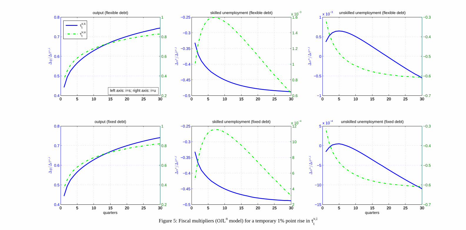
0 5 10 15 20 25 300.4

0.5

0.6

0.7

0.8output (flexible debt)

Δy/Δ

τ̃v,i

0 5 10 15 20 25 300.2

0.4

0.6

0.8

1

0 5 10 15 20 25 30−0.5

−0.45

−0.4

−0.35

−0.3

−0.25skilled unemployment (flexible debt)

Δss

/Δτ̃

v,i

0 5 10 15 20 25 300.6

0.8

1

1.2

1.4

1.6x 10

−3

0 5 10 15 20 25 30−1

−0.5

0

0.5

1x 10

−3 unskilled unemployment (flexible debt)

Δsu

/Δτ̃

v,i

0 5 10 15 20 25 30−0.7

−0.6

−0.5

−0.4

−0.3

0 5 10 15 20 25 300.4

0.5

0.6

0.7

0.8output (fixed debt)

Δy/Δ

τ̃v,i

quarters0 5 10 15 20 25 30

0.2

0.4

0.6

0.8

1

0 5 10 15 20 25 30−0.5

−0.45

−0.4

−0.35

−0.3

−0.25skilled unemployment (fixed debt)

Δss

/Δτ̃

v,i

0 5 10 15 20 25 302

4

6

8

10

12x 10

−4

0 5 10 15 20 25 30−15

−10

−5

0

5x 10

−4 unskilled unemployment (fixed debt)

Δsu

/Δτ̃

v,i

quarters

Figure 5: Fiscal multipliers (OJLn model) for a temporary 1% point rise in τv,it

0 5 10 15 20 25 30−0.7

−0.6

−0.5

−0.4

−0.3

τv,st

τv,ut

left axis: i=s; right axis: i=u

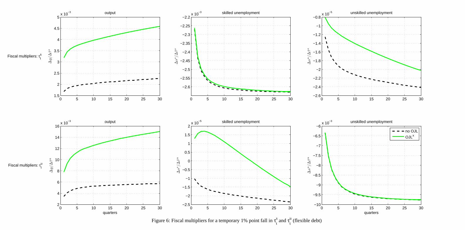
0 5 10 15 20 25 301.5

2

2.5

3

3.5

4

4.5

5x 10

−3 output

Δy/Δ

τ̃s

0 5 10 15 20 25 30

−2.6

−2.55

−2.5

−2.45

−2.4

−2.35

−2.3

−2.25

−2.2x 10

−3 skilled unemployment

Δss

/Δτ̃

s

0 5 10 15 20 25 30−2.6

−2.4

−2.2

−2

−1.8

−1.6

−1.4

−1.2

−1

−0.8x 10

−5 unskilled unemployment

Δsu

/Δτ̃

s

0 5 10 15 20 25 302

4

6

8

10

12

14

16x 10

−3 output

Δy/Δ

τ̃u

quarters0 5 10 15 20 25 30

−2.5

−2

−1.5

−1

−0.5

0

0.5

1

1.5

2x 10

−5 skilled unemployment

Δss

/Δτ̃

u

0 5 10 15 20 25 30−10

−9.5

−9

−8.5

−8

−7.5

−7

−6.5

−6x 10

−3 unskilled unemployment

Δsu

/Δτ̃

u

quarters

Fiscal multipliers: τst

Fiscal multipliers: τut

Figure 6: Fiscal multipliers for a temporary 1% point fall in τst and τu

t (flexible debt)

no OJL

OJLx