i

Modeling Basic Physical Links in

Acumen

Master report, IDE1252, June 2012

M

aster thesis

School of Inform

ation Science, Computer and Electrical Engineering

Muzeyen Hassen Esmael

ii

Modeling Basic Physical Links in Acumen

Master Thesis in Computer Network Engineering

June 2012

Author: Muzeyen Hassen Esmael Supervisor: Prof. Walid Taha Examiner: Prof. Tony Larsson

School of Information Science, Computer and Electrical Engineering Halmstad University

PO Box 823, SE-301 18 HALMSTAD, Sweden

iii

© Copyright Muzeyen Hassen Esmael, 2012. All rights reserved

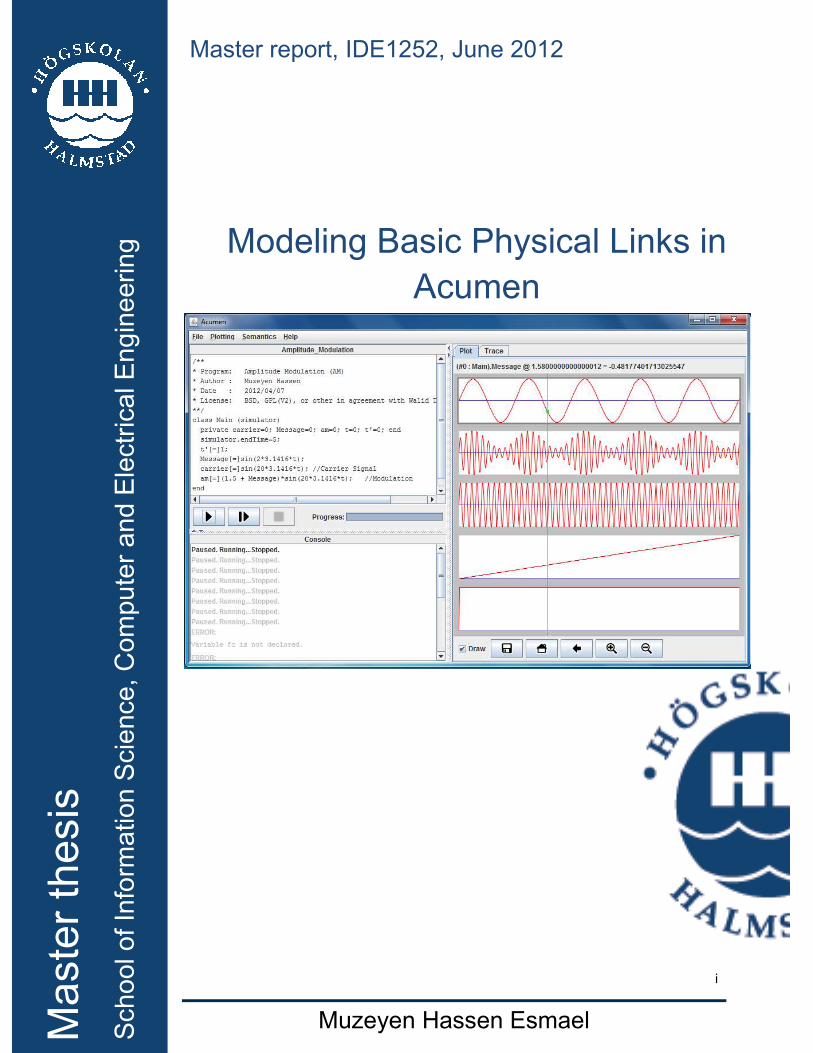
Master Thesis Report, IDE1252 School of Information Science, Computer and Electrical Engineering Halmstad University ISSN xxxxx Description of cover page picture:

The cover page picture shows Acumen model output for Amplitude Modulation system

iv

Abstract

Simulation is the process of computing a behavior determined by a given model of a system of interest. Modeling is the process of creating a model that formally describes a given class of system. Modeling and simulation can be used to quickly and cheaply study and understand new technologies. Today, a wide range of systems are simulated using different tools. However, converting models into simulation codes can still be difficult and time consuming. In this thesis, we study how a new modeling and simulation language called Acumen can be used to model basic physical links. This language is aimed at bridging the gap between modeling and simulation. We focus on basic physical links as an interesting type of system to model and simulate. We also focus on comparing Acumen to MATLAB and Simulink. The types of links we consider include models of an RC low-pass filter, Amplitude Modulation, Frequency Modulation, Amplitude Shift Keying, Phase Shift Keying and Frequency Shift Keying systems. Each of these examples is modeled in Acumen, MATLAB and Simulink. We find that, for the most part, Acumen allows us to naturally express a wide range of modulation techniques mentioned above. When compared to MATLAB ad Simulink, we find that Acumen is simple language to understand. Acumen codes are described in a more natural way. Simplicity is the biggest advantage of Acumen.

v

Acknowledgements

First and foremost, I would like to express my deepest gratitude to my advisor, Prof. Walid Taha, for his excellent supervision, guidance, care and assistance during the entire period of my thesis work. I would also like to thank Prof. Magnus Jonson (my co-advisor), Prof. Verónica Gaspes and Urban Bilstrup for the support they provided me throughout my thesis work. I would like to thank the School of Information Science, Computer and Electrical Engineering of Halmstad University for admitting me to its graduate program in Computer Network Engineering, which provided me an opportunity to advance my knowledge and skills in my area of specialization. I would also like to thank Haramaya University, Ethiopia, for providing me the required leave of absence for the period of my study. I'm grateful to Prof. Belay Kassa, Dr. Belaineh Legesse, Dr. Tena Alamirew and Tsehay Gelagil for their substantial support Furthermore, I am grateful to my best friends Dr. Hussein H. Komicha, Jeylan Wolyie, Adem Kedir and several others who have been providing me valuable advice and encouragements from the inception to the completion of my study. I would also like to thank my friends in Halmstad, Essayas G. Wahid, Mekuria Eyayu and Daniel Kifetew for the support they have provided me during my arrival in Halmstd and during my study. Finally, I would like to thank my wife, Meriyema Mohammed, my mother, father, brothers and sisters for their love, support, encouragement, and understanding.

vi

Table of Contents

Abstract ........................................................................................ iv

Acknowledgements ....................................................................... v

List of Figures ............................................................................... ix

List of Models ................................................................................ x

Chapter 1: Introduction .................................................................. 1

Introduction .............................................................................................. 1

Objective and Approach ........................................................................... 1

Related Work ........................................................................................... 1

Communication System Elements ........................................................... 2

Thesis Contributions ................................................................................ 2

Thesis Outline .......................................................................................... 3

Chapter 2: A Basic Acumen Tutorial ............................................. 4

Introduction .............................................................................................. 4

Variables .................................................................................................. 5

Comments and Punctuation ..................................................................... 6

Basic Operations and Mathematical functions .......................................... 6

Control Flow ............................................................................................. 7

Derivatives ............................................................................................... 9

Continuous Assignment ......................................................................... 10

Discrete Assignment .............................................................................. 10

Hybrid Behavior ..................................................................................... 10

Creating and Terminating Objects .......................................................... 10

Chapter 3: A Simple Channel Model ........................................... 12

Introduction ............................................................................................ 12

A Simple Acumen Model ........................................................................ 13

vii

Classes and Objects in Acumen ............................................................ 16

Simulink Model for Simple RC Channel ................................................. 17

Comparison between the Two Models ................................................... 19

Chapter 4: Amplitude Modulation ................................................ 21

Introduction ............................................................................................ 21

Amplitude Modulation and Demodulation ............................................... 21

Acumen Model for Amplitude Modulation ............................................... 22

MATLAB Model for Amplitude Modulation .............................................. 25

Simulink Model for Amplitude Modulation .............................................. 27

Comparison between the Three Models ................................................. 29

Chapter 5: Angular Modulation ................................................... 31

Introduction ............................................................................................ 31

Phase Modulation (PM) .......................................................................... 31

Frequency Modulation (FM) ................................................................... 31

Demodulation of PM and FM .................................................................. 32

Acumen Model for Frequency Modulation .............................................. 32

MATLAB Model for Frequency Modulation ............................................. 34

Simulink Model for Frequency Modulation ............................................. 37

Comparison Between The Three Models ............................................... 38

Chapter 6: Binary Amplitude Shift Keying ................................... 40

Digital Modulation Techniques ............................................................... 40

Binary Amplitude Shift Keying (BASK) ................................................... 40

Acumen Model for BASK Modulation ..................................................... 41

MATLAB Model for BASK Modulator and Demodulator ......................... 43

Simulink Model for BASK Modulator and Demodulator .......................... 47

Comparison between the Three Models ................................................. 49

Chapter 7: Binary Phase Shift Keying (BPSK) ............................ 51

viii

Binary Phase Shift Keying (BPSK) ......................................................... 51

Acumen Model for Binary Phase Shift Keying (BPSK) ........................... 51

MATLAB Model for Binary Phase Shift Keying (BPSK) .......................... 54

Simulink Model for Binary Phase Shift Keying (BPSK) ........................... 57

Comparison between the Three Models ................................................. 59

Chapter 8: Binary Frequency Shift Keying (BFSK) ..................... 60

Binary Frequency Shift Keying (BFSK) .................................................. 60

Acumen Model for Binary Frequency Shift Keying (BFSK) ..................... 60

MATLAB Model for Binary Frequency Shift Keying (BFSK) .................... 64

Simulink Model for Binary Frequency Shift Keying (BFSK) .................... 68

Comparison between the Three Models ................................................. 69

Chapter 9: Conclusion and Future Work ..................................... 70

Future Works ......................................................................................... 75

References .................................................................................. 76

Appendix ..................................................................................... 78

Collection of Acumen Codes ..................................................................... 78

ix

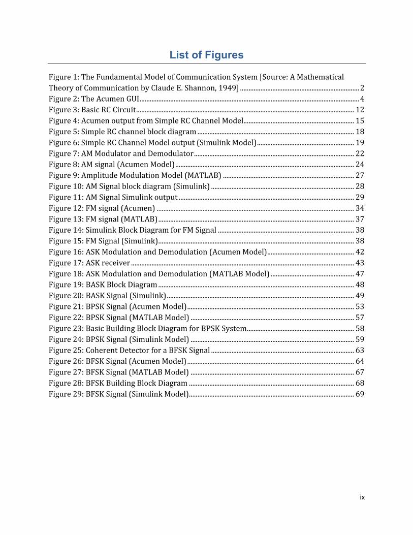
List of Figures

Figure 1: The Fundamental Model of Communication System [Source: A Mathematical Theory of Communication by Claude E. Shannon, 1949] ...................................................................... 2 Figure 2: The Acumen GUI ................................................................................................................................. 4 Figure 3: Basic RC Circuit ................................................................................................................................ 12 Figure 4: Acumen output from Simple RC Channel Model................................................................. 15 Figure 5: Simple RC channel block diagram ............................................................................................ 18 Figure 6: Simple RC Channel Model output (Simulink Model) ......................................................... 19 Figure 7: AM Modulator and Demodulator .............................................................................................. 22 Figure 8: AM signal (Acumen Model) ......................................................................................................... 24 Figure 9: Amplitude Modulation Model (MATLAB) ............................................................................. 27 Figure 10: AM Signal block diagram (Simulink) .................................................................................... 28 Figure 11: AM Signal Simulink output ....................................................................................................... 29 Figure 12: FM signal (Acumen) .................................................................................................................... 34 Figure 13: FM signal (MATLAB) ................................................................................................................... 37 Figure 14: Simulink Block Diagram for FM Signal ................................................................................ 38 Figure 15: FM Signal (Simulink) ................................................................................................................... 38 Figure 16: ASK Modulation and Demodulation (Acumen Model) ................................................... 42 Figure 17: ASK receiver ................................................................................................................................... 43 Figure 18: ASK Modulation and Demodulation (MATLAB Model) ................................................. 47 Figure 19: BASK Block Diagram ................................................................................................................... 48 Figure 20: BASK Signal (Simulink) .............................................................................................................. 49 Figure 21: BPSK Signal (Acumen Model) .................................................................................................. 53 Figure 22: BPSK Signal (MATLAB Model) ................................................................................................ 57 Figure 23: Basic Building Block Diagram for BPSK System ............................................................... 58 Figure 24: BPSK Signal (Simulink Model) ................................................................................................ 59 Figure 25: Coherent Detector for a BFSK Signal .................................................................................... 63 Figure 26: BFSK Signal (Acumen Model) .................................................................................................. 64 Figure 27: BFSK Signal (MATLAB Model) ................................................................................................ 67 Figure 28: BFSK Building Block Diagram ................................................................................................. 68 Figure 29: BFSK Signal (Simulink Model) ................................................................................................. 69

x

List of Models

Model 1: Acumen Model for a simple channel ........................................................................................ 13 Model 2: A more Modular Acumen Model for simple RC channel .................................................. 16 Model 3: Acumen Model for Amplitude Modulation ............................................................................ 22 Model 4: MATLAB Model for Amplitude Modulation ........................................................................... 25 Model 5: Acumen Model for FM Signal ...................................................................................................... 32 Model 6: MATLAB Model for Frequency Modulation .......................................................................... 35 Model 7: Acumen Model for BASK ............................................................................................................... 41 Model 8: MATLAB Model for BASK ............................................................................................................. 43 Model 9: Acumen Model for BPSK ............................................................................................................... 51 Model 10: MATLAB Model for BPSK ........................................................................................................... 54 Model 11: BFSK Signal with non-coherent detection (Acumen Model) ....................................... 60 Model 12: BFSK Signal with coherent detection (Acumen Model) ................................................. 62 Model 13: BFSK Signal (MATLAB Model) ................................................................................................. 64

1

Chapter 1: Introduction

Introduction

In building any simple or complex communication network systems, it is clear that it is very costly to buy real network devices and tools required to establish or deploy a complete system. In addition, it is difficult to deploy tested systems without having the real equipment, such as computers, switches, routers, oscilloscopes and also the different software required for the systems. To overcome these problems, researchers and software engineers developed different network simulation tools that can help design complete network systems. Network simulators enable researchers, network administrators, and other interested users to test new network technologies and protocols before using them on real networks; thus, saving a lot of time and money. In this thesis, we will study basic examples of physical link modeling and simulation of network systems using a new and small executable modeling language called Acumen [1]. Acumen is a new language for modeling and simulation of hybrid (discrete/continuous) systems, currently being developed by Prof. Walid Taha and other collaborators. This is the first thesis that evaluates the design of Acumen (Version 10). Because of this, the work of the thesis started from basic models of physical links in a communication system.

Objective and Approach

The main purpose of this thesis is to examine and discover how basic physical links of network systems are modeled in Acumen. Thus, the analysis of Acumen as a modeling and simulation tool and Acumen code examples are the main focus of the thesis. This includes presenting several Acumen codes in the thesis, discussing and evaluating the extent to which Acumen language makes modeling such components convenient. The thesis has tutorial content that explains clearly to the reader how the codes and other features of the language are interpreted and also explains how network components can be modeled in this language. In focus on modeling very small and simple examples and on case studies to identify the advantages and disadvantages of using Acumen is compared to using other modeling tools, such as MATLAB and Simulink.

Related Work

In this section, we will discuss some popular tools that serve a similar purpose to Acumen. Each of these tools is based on different technologies. Some of them are based on block diagrams while others are based on functional programming. In tools based on block diagrams, different systems are represented with block diagrams. Simulink and VisSim can

2

be good examples of dynamical systems simulation tools based on block diagram. VisSim is a block diagram language for creating complex nonlinear dynamic systems [2]. To create a model in VisSim, one can simply drag and drop the blocks required for the model into the workspace and connect them with wires. In addition, this tool provides the option to display the plots in 2D or 3D. The other popular tool used for modeling dynamical systems is MATLAB. In this thesis, we will use MATLAB and Simulink and compare Acumen models with them.

Communication System Elements

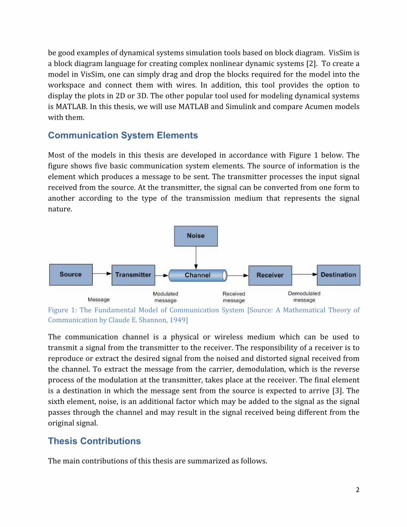
Most of the models in this thesis are developed in accordance with Figure 1 below. The figure shows five basic communication system elements. The source of information is the element which produces a message to be sent. The transmitter processes the input signal received from the source. At the transmitter, the signal can be converted from one form to another according to the type of the transmission medium that represents the signal nature.

Figure 1: The Fundamental Model of Communication System [Source: A Mathematical Theory of Communication by Claude E. Shannon, 1949]

The communication channel is a physical or wireless medium which can be used to transmit a signal from the transmitter to the receiver. The responsibility of a receiver is to reproduce or extract the desired signal from the noised and distorted signal received from the channel. To extract the message from the carrier, demodulation, which is the reverse process of the modulation at the transmitter, takes place at the receiver. The final element is a destination in which the message sent from the source is expected to arrive [3]. The sixth element, noise, is an additional factor which may be added to the signal as the signal passes through the channel and may result in the signal received being different from the original signal.

Thesis Contributions

The main contributions of this thesis are summarized as follows.

3

� We illustrate the basic utility of Acumen as a modeling and simulation tool using a series of modulation/demodulation methods as case studies. We carry out this study in the context of a simple, first-order RC model of a communication channel. We find that, for the most part, Acumen allows us to naturally express a wide range of modulation techniques, including AM modulation, FM modulation, Amplitude Shift Keying, Phase Shift Keying and Frequency Shift Keying modulations.

� To identify some ways in which Acumen is better than other related tools, we build Acumen models in MATLAB and Simulink. We compare the results of Acumen, MATLAB and Simulink based on the plots they generate. The plots show similarity in most of the models we build in this thesis.

Thesis Outline

In this chapter, we introduced the basic research question that need to be answered in the thesis and indicated the approach followed during the process of the study. The second chapter presents basic tutorial on Acumen. Chapters 3 through 8 are the technical core to the thesis. The third chapter presents a model of simple RC low-pass filter model. The example presented in the first part of this chapter is further extended and investigated in a different approach. In addition, it addresses how the Acumen code is interpreted by the compiler. The RC low-pass filter is also modeled with Simulink. In Chapter 4, Amplitude Modulation system is modeled in three different tools including Acumen, MATLAB and Simulink. The fifth chapter presents a model for Frequency Modulation system with the three tools mentioned above. In chapters 6, 7 and 8, the models for digital modulation techniques namely, Amplitude Shift Keying, Phase Shift Keying and Frequency Shift Keying have been presented respectively in Acumen, MATLAB and Simulink.

Finally, the last chapter discusses the conclusion and future research work and followed by references and appendix (Acumen codes).

Chapter 2:

Introduction

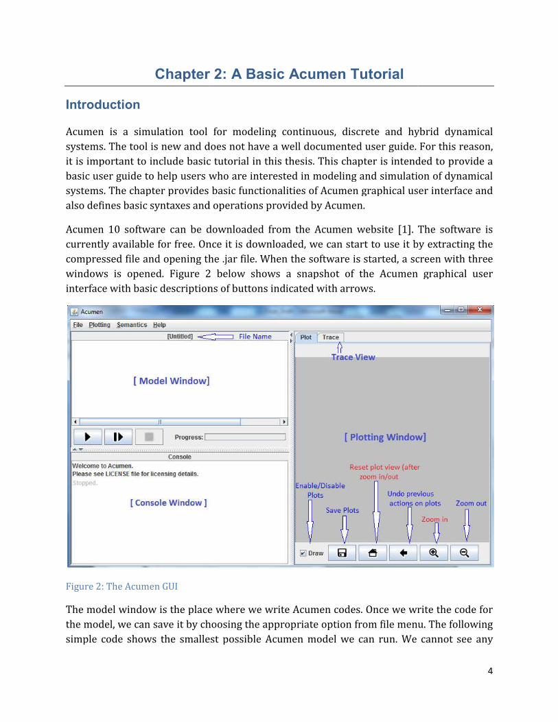
Acumen is a simulation tool for modeling continuous, discrete and hybrid dynamical systems. The tool is new and does not have a well documented user guide. it is important to include basic tutorial in this thesis. basic user guide to help users who are systems. The chapter provides basic functionalities of Acumen graphical also defines basic syntaxes and operations provided by Acumen.

Acumen 10 software can be downloaded from the Acumen websitecurrently available for free. Once it is downloaded, we can start to use it by extracting the compressed file and opening the .jar file. When the software is started, a screen with three windows is opened. Figure 2interface with basic descriptions of buttons indicated with arrows.

Figure 2: The Acumen GUI

The model window is the place where we write Acumen codes. Once we write the code fthe model, we can save it by choosing the appropriate option from file menu. The following simple code shows the smallest possible Acumen model we can run. We cannot see any

Chapter 2: A Basic Acumen Tutorial

Acumen is a simulation tool for modeling continuous, discrete and hybrid dynamical systems. The tool is new and does not have a well documented user guide. it is important to include basic tutorial in this thesis. This chapter is intended

users who are interested in modeling and simulation of dynamical systems. The chapter provides basic functionalities of Acumen graphical user interface

basic syntaxes and operations provided by Acumen.

software can be downloaded from the Acumen website [1]. currently available for free. Once it is downloaded, we can start to use it by extracting the compressed file and opening the .jar file. When the software is started, a screen with three

2 below shows a snapshot of the Acumen graphical user interface with basic descriptions of buttons indicated with arrows.

The model window is the place where we write Acumen codes. Once we write the code fthe model, we can save it by choosing the appropriate option from file menu. The following simple code shows the smallest possible Acumen model we can run. We cannot see any

4

Acumen is a simulation tool for modeling continuous, discrete and hybrid dynamical systems. The tool is new and does not have a well documented user guide. For this reason,

This chapter is intended to provide a in modeling and simulation of dynamical

user interface and

. The software is currently available for free. Once it is downloaded, we can start to use it by extracting the compressed file and opening the .jar file. When the software is started, a screen with three

below shows a snapshot of the Acumen graphical user

The model window is the place where we write Acumen codes. Once we write the code for the model, we can save it by choosing the appropriate option from file menu. The following simple code shows the smallest possible Acumen model we can run. We cannot see any

5

output from this model. However, it is the simplest code that can be executed without error.

class Main(simulator) end

This simple model can be described as follows. The first line shows the mandatory main class declaration. The class Main() with simulator as a parameter always represents the whole system that we model. The simulator parameter allows users to define the behavior of the model. For example, users can define the simulation start time, end time, and step size

as shown below.

class Main (simulator) private /*…Variables Declaration and initialization .. */ end simulator.startTime = 2.0; simulator.timeStep = 0.001; simulator.endTime = 5.0; // ... the rest of model ... end

The second line in the above table always begins with a key word ‘private’ and ends with the key word ‘end’. Variables that we need to use in the model are always declared and initialized in between these words. The last line shows the end of class Main().

Variables

Variables in Acumen have the same purpose as variables in other languages. All variables defined in Acumen are functions of time. These variables are declared in the private section of Acumen code and they must be initialized and are accessible throughout the class. If more than one variable is used in the model, they are separated with a semicolon. For example, we can declare and initialize variable X, Y and Z as follows:

class Main(simulator) private X=0; Y=1; Z=10 end end

Once these variables are declared and initialized, we can see the plots of these variables in the right side window when we run the model using ‘Run Simulation’ button. Acumen has rules about variable names. Acumen variables are case sensitive. This means that variable x is different from block letter X. Variable names must begin with letters (A to Z or a to z) or

6

underscores. After the first character in the variable, variable names can have any combination of characters. Acumen also supports special variables that are differentiated from normal variables by having primes ( ’ ) at the end. These variables represent derivatives of variables. For example, X’ and X’’ represent the first and second derivatives of X with respect to time respectively. Acumen keywords (reserved words) like if, else,

switch, case, end, for, sum, class, private, create, terminate, stop etc cannot be used as variable names.

Comments and Punctuation

Acumen supports single line and multi-line comments. In Acumen, the symbol // is used to comment a single line and /* … */ is used to comment multiple lines. Comments are usually added for the purpose of making Acumen codes easier to understand. This means that any line of Acumen code that starts with // symbol or placed between /* … */ will not be executed.

The most commonly used punctuation mark is semicolon. In Acumen, a semicolon is used to separate variables declared in the private section. It is also placed at the end of Acumen codes to separate different commands.

Basic Operations and Mathematical functions

Acumen provides many operations to manipulate given variables. These include arithmetic operation, relational operations, logical operations, bitwise operations, assignment operations and vector operations. The following table summarizes some of these operations with examples.

Arithmetic Operators (Assume X=10 and Y=20)

Operator Description Example (How we write in Acumen)

+ Binary addition X + Y gives 30

- Binary Subtraction X - Y gives -10

* Binary Multiplication X * Y gives 200

/ Binary Division X / Y gives 0.5

% Modulus X % Y gives 10

Relational Operators (Assume X=10 and Y=20)

== Relational equality (X == Y) is not true

!= Not equal to (X != Y) is true

> Greater than (X > Y) is not true

7

< Less than (X < Y) is true

>= Greater than or equal to

(X >= Y) is not true

<= Less than or equal to (X <= Y) is true

Logical (Boolean) operators (Assume X and Y are Boolean expressions)

&& Logical and X && Y (returns true if both X and Y are true)

|| Logical or X || Y (returns true if either X or Y is true)

Assignment Operations

= Discrete assignment Z = X (Assigns the value of X to Z)

[=] Continuous assignment

Z[=]X (similar to discrete assignment)

Continuous integration (for any number of primes)

Z’[=]X (Z changes over time at the rate of X)

Acumen also supports some mathematical functions that can be used in modeling different systems. These functions are included as built-in functions in Acumen and are ready for use. The basic mathematical functions available with Acumen are listed in the table below.

Function Description Example (How we write in

Acumen) Assume (x = 25)

abs Absolute value or Magnitude y = abs(x) gives 25

sin Sine function y = sin(x) gives 0.132351750097

cos Cosine function y = cos(x) gives 0.99120281186

sqrt Square root y = sqrt(x) gives 5

^ Power x^2 (x to the power of 2) gives 625

Control Flow

Acumen provides different control flow structures including if-else-end, switch-case and for-loops. The syntax for each of these decision-making structures is similar to the syntax used in other programming languages. The following table shows the syntax for these control flow statements in Acumen models.

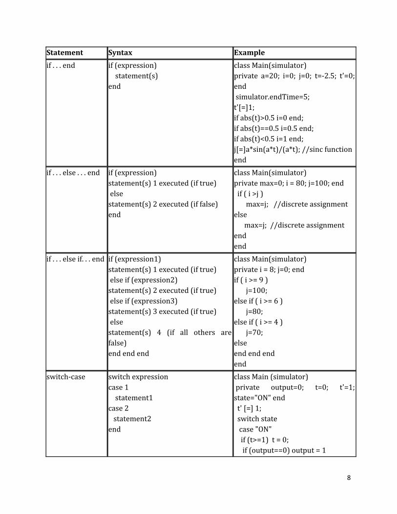
8

Statement Syntax Example

if . . . end if (expression) statement(s) end

class Main(simulator) private a=20; i=0; j=0; t=-2.5; t'=0; end simulator.endTime=5; t'[=]1; if abs(t)>0.5 i=0 end; if abs(t)==0.5 i=0.5 end; if abs(t)<0.5 i=1 end; j[=]a*sin(a*t)/(a*t); //sinc function end

if . . . else . . . end if (expression) statement(s) 1 executed (if true) else statement(s) 2 executed (if false) end

class Main(simulator) private max=0; i = 80; j=100; end if ( i >j ) max=j; //discrete assignment else max=j; //discrete assignment end end

if . . . else if. . . end if (expression1) statement(s) 1 executed (if true) else if (expression2) statement(s) 2 executed (if true) else if (expression3) statement(s) 3 executed (if true) else statement(s) 4 (if all others are false) end end end

class Main(simulator) private i = 8; j=0; end if ( i >= 9 ) j=100; else if ( i >= 6 ) j=80; else if ( i >= 4 ) j=70; else end end end end

switch-case switch expression case 1 statement1 case 2 statement2 end

class Main (simulator) private output=0; t=0; t'=1; state="ON" end t' [=] 1; switch state case "ON" if (t>=1) t = 0; if (output==0) output = 1

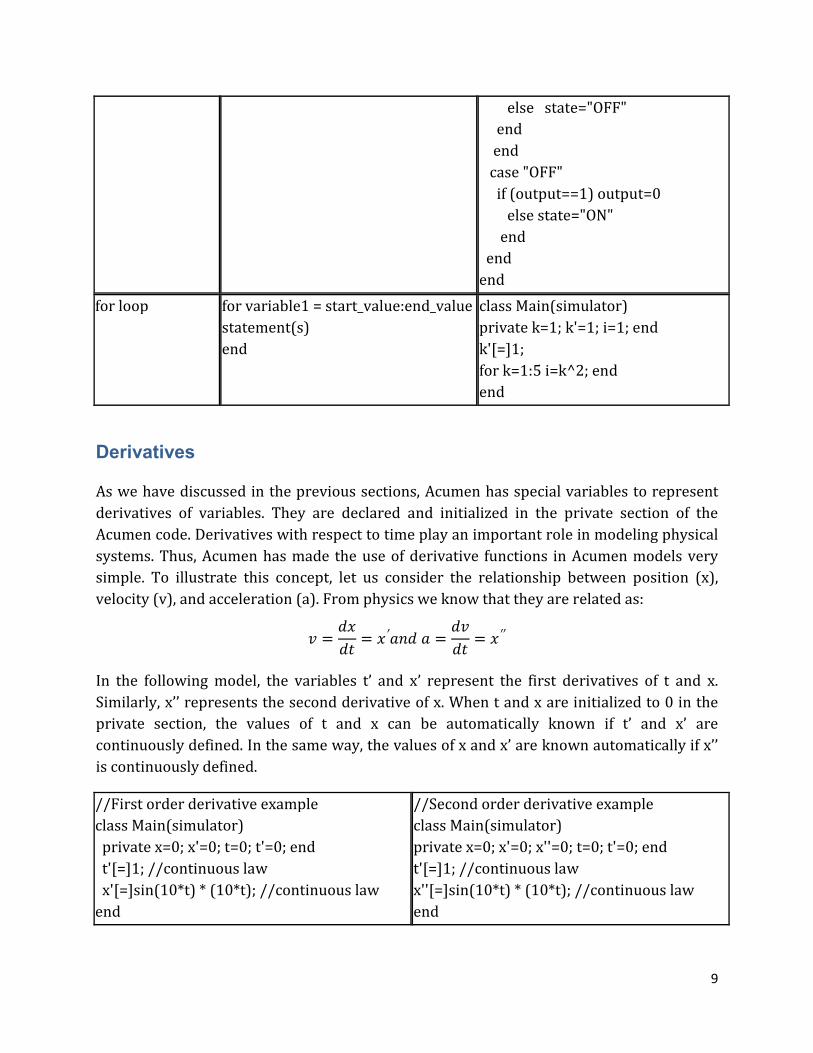
9

else state="OFF" end end case "OFF" if (output==1) output=0 else state="ON" end end end

for loop for variable1 = start_value:end_value statement(s) end

class Main(simulator) private k=1; k'=1; i=1; end k'[=]1; for k=1:5 i=k^2; end end

Derivatives

As we have discussed in the previous sections, Acumen has special variables to represent derivatives of variables. They are declared and initialized in the private section of the Acumen code. Derivatives with respect to time play an important role in modeling physical systems. Thus, Acumen has made the use of derivative functions in Acumen models very simple. To illustrate this concept, let us consider the relationship between position (x), velocity (v), and acceleration (a). From physics we know that they are related as:

� = ���� = �′���� = ���� = �

′′

In the following model, the variables t’ and x’ represent the first derivatives of t and x. Similarly, x’’ represents the second derivative of x. When t and x are initialized to 0 in the private section, the values of t and x can be automatically known if t’ and x’ are continuously defined. In the same way, the values of x and x’ are known automatically if x’’ is continuously defined.

//First order derivative example class Main(simulator) private x=0; x'=0; t=0; t'=0; end t'[=]1; //continuous law x'[=]sin(10*t) * (10*t); //continuous law end

//Second order derivative example class Main(simulator) private x=0; x'=0; x''=0; t=0; t'=0; end t'[=]1; //continuous law x''[=]sin(10*t) * (10*t); //continuous law end

10

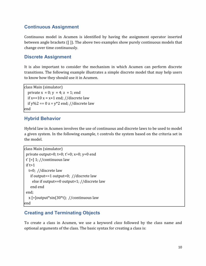
Continuous Assignment

Continuous model in Acumen is identified by having the assignment operator inserted between angle brackets ([ ]). The above two examples show purely continuous models that change over time continuously.

Discrete Assignment

It is also important to consider the mechanism in which Acumen can perform discrete transitions. The following example illustrates a simple discrete model that may help users to know how they should use it in Acumen.

class Main (simulator) private x = 0; y = 4; z = 1; end if x==10 x = x+1 end; //discrete law if y%2 == 0 z = y*2 end; //discrete law end

Hybrid Behavior

Hybrid law in Acumen involves the use of continuous and discrete laws to be used to model a given system. In the following example, t controls the system based on the criteria set in the model.

class Main (simulator) private output=0; t=0; t'=0; x=0; y=0 end t' [=] 1; //continuous law if t>1 t=0; //discrete law if output==1 output=0; //discrete law else if output==0 output=1; //discrete law end end end; x [=]output*sin(30*t); //continuous law end

Creating and Terminating Objects

To create a class in Acumen, we use a keyword class followed by the class name and optional arguments of the class. The basic syntax for creating a class is:

11

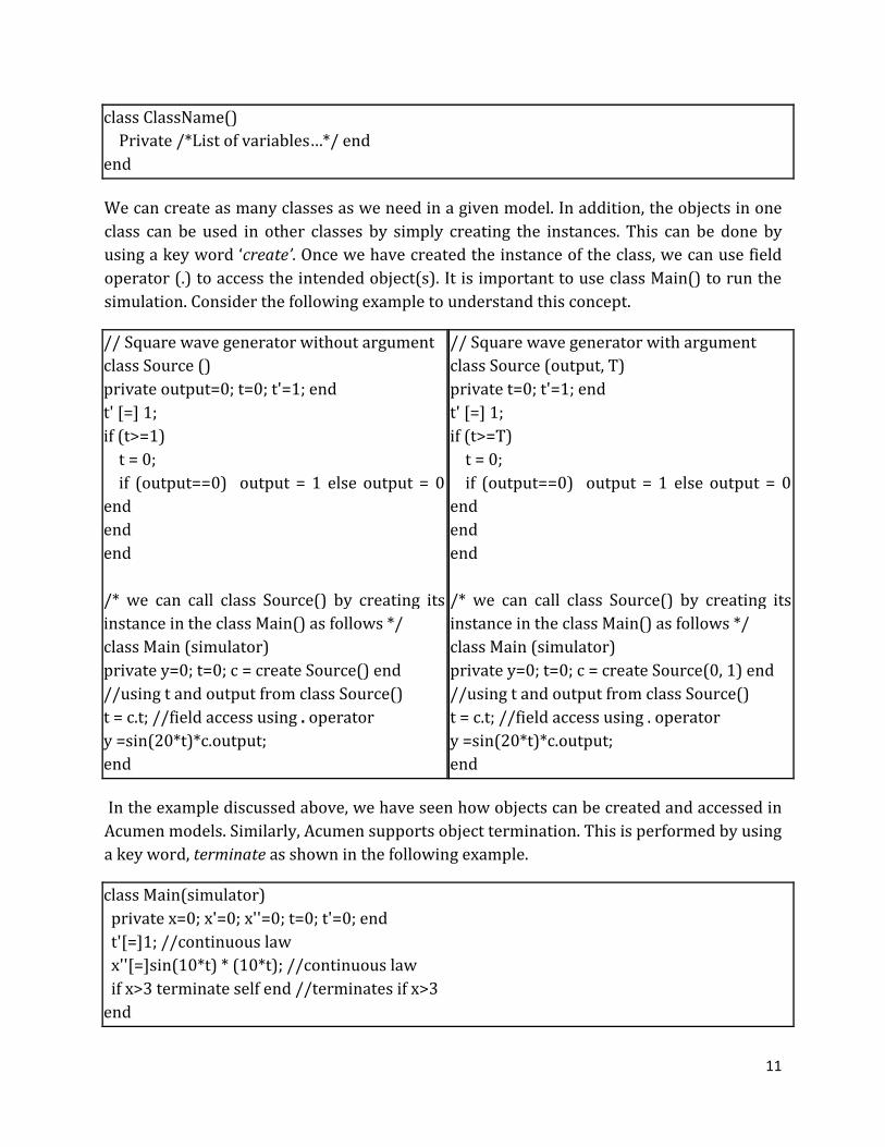
class ClassName() Private /*List of variables…*/ end end

We can create as many classes as we need in a given model. In addition, the objects in one class can be used in other classes by simply creating the instances. This can be done by using a key word ‘create’. Once we have created the instance of the class, we can use field operator (.) to access the intended object(s). It is important to use class Main() to run the simulation. Consider the following example to understand this concept.

// Square wave generator without argument class Source () private output=0; t=0; t'=1; end t' [=] 1; if (t>=1) t = 0; if (output==0) output = 1 else output = 0 end end end /* we can call class Source() by creating its instance in the class Main() as follows */ class Main (simulator) private y=0; t=0; c = create Source() end //using t and output from class Source() t = c.t; //field access using . operator y =sin(20*t)*c.output; end

// Square wave generator with argument class Source (output, T) private t=0; t'=1; end t' [=] 1; if (t>=T) t = 0; if (output==0) output = 1 else output = 0 end end end /* we can call class Source() by creating its instance in the class Main() as follows */ class Main (simulator) private y=0; t=0; c = create Source(0, 1) end //using t and output from class Source() t = c.t; //field access using . operator y =sin(20*t)*c.output; end

In the example discussed above, we have seen how objects can be created and accessed in Acumen models. Similarly, Acumen supports object termination. This is performed by using a key word, terminate as shown in the following example.

class Main(simulator) private x=0; x'=0; x''=0; t=0; t'=0; end t'[=]1; //continuous law x''[=]sin(10*t) * (10*t); //continuous law if x>3 terminate self end //terminates if x>3 end

12

Chapter 3: A Simple Channel Model

Introduction

In practice, it is the responsibility of a communication system to transmit information from source to destination. The original information signal passes through different communication system components and then undergoes so many changes in its orientation and shape because of noise and attenuation. As discussed in the first chapter, a communication system consists of source of information, transmitter, transmission medium (channel), receiver and destination (sink).

To reach its destination, the signal generated by the source of information needs to pass through a certain medium of communication. Depending on the capacity of the channel (medium) used; the signal can be either detected or undetected at the destination. This is because of different factors which the signal encounters as it passes through the channel.

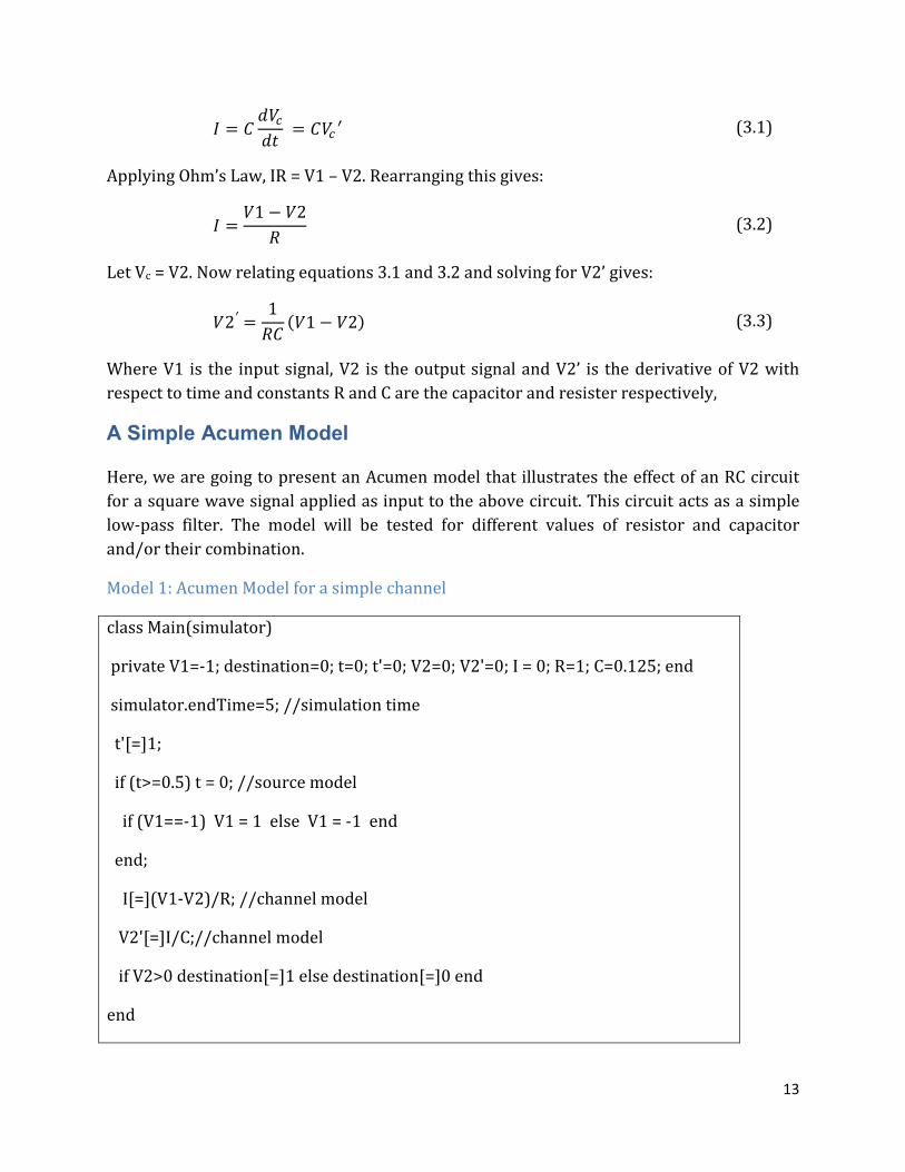
This chapter presents a simple channel model consisting of a basic first order RC circuit as shown in Figure 3. The model illustrates how this RC circuit affects the shape and strength of the output signal. A first order RC circuit consists of a resister and a capacitor and can be used to filter a signal. There are two most commonly used RC filters known as low-pass and high-pass filters. The low-pass filter allows low frequency components of a signal to pass without attenuation while blocking the others. On the other hand, the high-pass filter does the reverse. In the following section, we will model a low-pass filter in Acumen and Simulink and compare the results obtained with these tools.

Figure 3: Basic RC Circuit

When the input voltage, V1 applied to the above circuit is DC source, there will be no current flow through the capacitor. This is because the capacitor blocks DC. However, when a voltage that varies over time is applied as input, the current flowing through the capacitor can be expressed as:

13

= ����� = ��′ (3.1)

Applying Ohm’s Law, IR = V1 – V2. Rearranging this gives:

= �1 − �2� (3.2)

Let Vc = V2. Now relating equations 3.1 and 3.2 and solving for V2’ gives:

�2′ = 1� ��1 − �2� (3.3)

Where V1 is the input signal, V2 is the output signal and V2’ is the derivative of V2 with respect to time and constants R and C are the capacitor and resister respectively,

A Simple Acumen Model

Here, we are going to present an Acumen model that illustrates the effect of an RC circuit for a square wave signal applied as input to the above circuit. This circuit acts as a simple low-pass filter. The model will be tested for different values of resistor and capacitor and/or their combination.

Model 1: Acumen Model for a simple channel

class Main(simulator)

private V1=-1; destination=0; t=0; t'=0; V2=0; V2'=0; I = 0; R=1; C=0.125; end

simulator.endTime=5; //simulation time

t'[=]1;

if (t>=0.5) t = 0; //source model

if (V1==-1) V1 = 1 else V1 = -1 end

end;

I[=](V1-V2)/R; //channel model

V2'[=]I/C;//channel model

if V2>0 destination[=]1 else destination[=]0 end

end

14

The above model can be described as follows. The // symbol in the above model shows a comment which is usually added for the purpose of making Acumen codes easier to understand. This means that any line of Acumen code that starts with this symbol will not be executed. All variables defined in this example are functions of time. These variables are declared in the private section of the Acumen code and they must be initialized and are accessible throughout the class.

When variables are declared with primes (’), they represent the derivative with respect to time [4]. In the model above, the variables t’ and V2’ represent the derivatives of t and V2 respectively. In this case, since t and V2 have been initialized to 0 in the private section, the values of t and V2 can be automatically known as t’ and V2’ are continuously defined.

The statement ‘simulator.endTime=5’ sets the total simulation time to 5. Line 4 in the model shows continuous assignment. This means that the rate at which t changes is 1 and t’ is always 1. On the other hand, t=0 indicates discrete assignment which means that t is always reset to zero when the condition in the outer if statement is satisfied. Similarly, when the condition in the outer if statement is satisfied the inner if statement will be executed. In the inner if statement, there is a discrete state controller that decides whether the input signal, V1 is -1 or 1. If V1 is at position -1, the signal moves from position -1 to 1, otherwise, it moves from position 1 to -1.

The variable V1 is the input to the system while V2 is the output. The constant variables R and C represent the resistance and the capacitance of the cable (channel) respectively. As can be seen from this model, at t=0, the initial condition for variables V1, V2 and I is also zero. After a short time, when the flow of current starts, the capacitor starts to charge up and results in increasing V2 exponentially. This also results in exponential decay in V2’ and current, I. From this we can prove that the current flowing around the circuit is proportional to the derivative of V2 multiplied by capacitor, C. As the process continues, the voltage across the capacitor, V2 starts to decrease exponentially while V2’ and I increase exponentially.

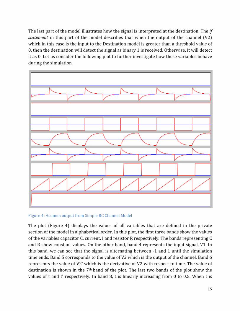
The last part of the model illustrates how the signal istatement in this part of the model describes that when the output of the channel (V2) which in this case is the input to the Destination model is greater than a threshold value of 0, then the destination will detecit as 0. Let us consider the following plot to further investigate how these variables behave during the simulation.

Figure 4: Acumen output from Simple RC Channel

The plot (Figure 4) displays the values of all variables that are defined in the private section of the model in alphabetical order. In this plot, the first three bands show the values of the variables capacitor C, current, I and resistor R respectivand R show constant values. On the other hand, band 4 represents the input signal, V1. In this band, we can see that the signal is alternating between time ends. Band 5 corresponds to the value ofrepresents the value of V2’ which is the derivative of V2 with respect to time. The value of destination is shown in the 7th

values of t and t’ respectively. In band 8,

The last part of the model illustrates how the signal is interpreted at the destination. The in this part of the model describes that when the output of the channel (V2)

which in this case is the input to the Destination model is greater than a threshold value of 0, then the destination will detect the signal as binary 1 is received. Otherwise, it will detect it as 0. Let us consider the following plot to further investigate how these variables behave

: Acumen output from Simple RC Channel Model

) displays the values of all variables that are defined in the private section of the model in alphabetical order. In this plot, the first three bands show the values of the variables capacitor C, current, I and resistor R respectively. The bands representing C and R show constant values. On the other hand, band 4 represents the input signal, V1. In this band, we can see that the signal is alternating between -1 and 1 until the simulation time ends. Band 5 corresponds to the value of V2 which is the output of the channel. Band 6 represents the value of V2’ which is the derivative of V2 with respect to time. The value of

th band of the plot. The last two bands of the plot show the ively. In band 8, t is linearly increasing from 0 to 0.5

15

s interpreted at the destination. The if in this part of the model describes that when the output of the channel (V2)

which in this case is the input to the Destination model is greater than a threshold value of t the signal as binary 1 is received. Otherwise, it will detect

it as 0. Let us consider the following plot to further investigate how these variables behave

) displays the values of all variables that are defined in the private section of the model in alphabetical order. In this plot, the first three bands show the values

ely. The bands representing C and R show constant values. On the other hand, band 4 represents the input signal, V1. In

1 and 1 until the simulation V2 which is the output of the channel. Band 6

represents the value of V2’ which is the derivative of V2 with respect to time. The value of band of the plot. The last two bands of the plot show the

o 0.5. When t is

16

greater than or equal to 0.5, t is again reset to 0. Since the rate of change in t is 1 in the model, one can clearly see that the value of t’ in the last band is always 1.

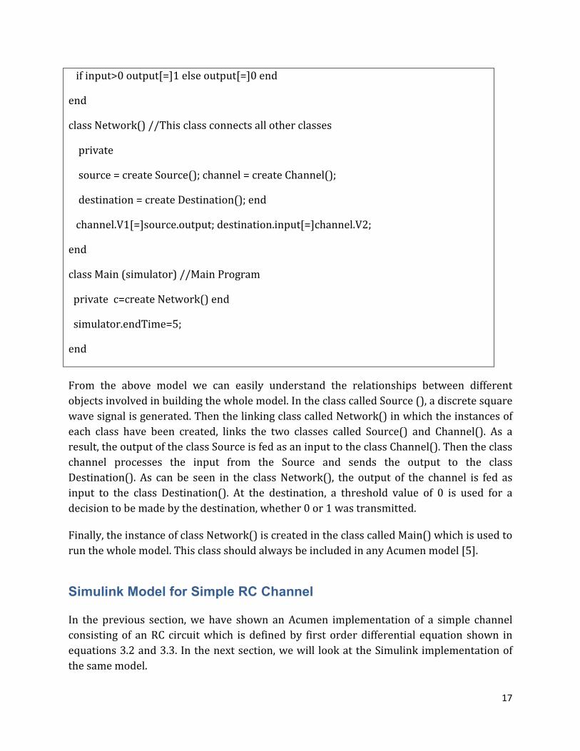
Classes and Objects in Acumen

In Acumen, objects are the main abstraction techniques used. They are introduced by including a class declaration in the model. This enables us to break down a big model to make it suitable, manageable and easy to understand. Each module or object accomplishes its own functions. Each object can then be organized into one big model through another object or class that links them together. In the class that connects different classes and objects, we simply use a create statement to create individual objects as instances of each class. This feature in Acumen helps to build a clear and easy to understand model of different systems. The following example illustrates the process of implementing the simple RC filter model, discussed in the earlier section, in a modular approach.

Model 2: A more Modular Acumen Model for simple RC channel

class Source() //Source model

private output=-1; t=0; t'=0; end

t'[=]1;

if (t>=0.5) t = 0;

if (output==-1 ) output = 1 else output = -1 end

end;

end

class Channel() //Channel model

private V1=0; V2=0; V2'=0; I = 0; R=1; C=0.125; end

I[=](V1-V2)/R; //channel model

V2'[=]I/C;//channel model

end

class Destination() //Destination model

private input=0; output=0 end

17

if input>0 output[=]1 else output[=]0 end

end

class Network() //This class connects all other classes

private

source = create Source(); channel = create Channel();

destination = create Destination(); end

channel.V1[=]source.output; destination.input[=]channel.V2;

end

class Main (simulator) //Main Program

private c=create Network() end

simulator.endTime=5;

end

From the above model we can easily understand the relationships between different objects involved in building the whole model. In the class called Source (), a discrete square wave signal is generated. Then the linking class called Network() in which the instances of each class have been created, links the two classes called Source() and Channel(). As a result, the output of the class Source is fed as an input to the class Channel(). Then the class channel processes the input from the Source and sends the output to the class Destination(). As can be seen in the class Network(), the output of the channel is fed as input to the class Destination(). At the destination, a threshold value of 0 is used for a decision to be made by the destination, whether 0 or 1 was transmitted.

Finally, the instance of class Network() is created in the class called Main() which is used to run the whole model. This class should always be included in any Acumen model [5].

Simulink Model for Simple RC Channel

In the previous section, we have shown an Acumen implementation of a simple channel consisting of an RC circuit which is defined by first order differential equation shown in equations 3.2 and 3.3. In the next section, we will look at the Simulink implementation of the same model.

18

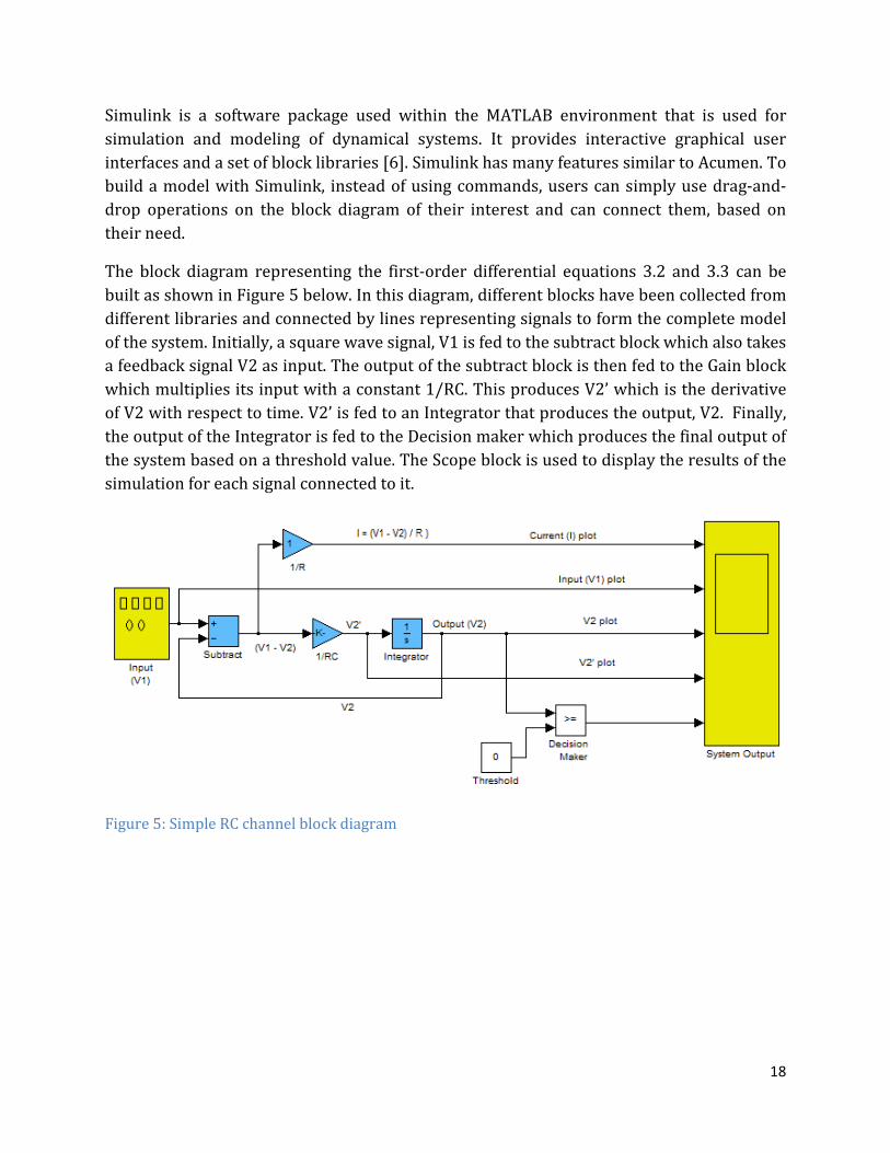
Simulink is a software package used within the MATLAB environment that is used for simulation and modeling of dynamical systems. It provides interactive graphical user interfaces and a set of block libraries [6]. Simulink has many features similar to Acumen. To build a model with Simulink, instead of using commands, users can simply use drag-and-drop operations on the block diagram of their interest and can connect them, based on their need.

The block diagram representing the first-order differential equations 3.2 and 3.3 can be built as shown in Figure 5 below. In this diagram, different blocks have been collected from different libraries and connected by lines representing signals to form the complete model of the system. Initially, a square wave signal, V1 is fed to the subtract block which also takes a feedback signal V2 as input. The output of the subtract block is then fed to the Gain block which multiplies its input with a constant 1/RC. This produces V2’ which is the derivative of V2 with respect to time. V2’ is fed to an Integrator that produces the output, V2. Finally, the output of the Integrator is fed to the Decision maker which produces the final output of the system based on a threshold value. The Scope block is used to display the results of the simulation for each signal connected to it.

Figure 5: Simple RC channel block diagram

19

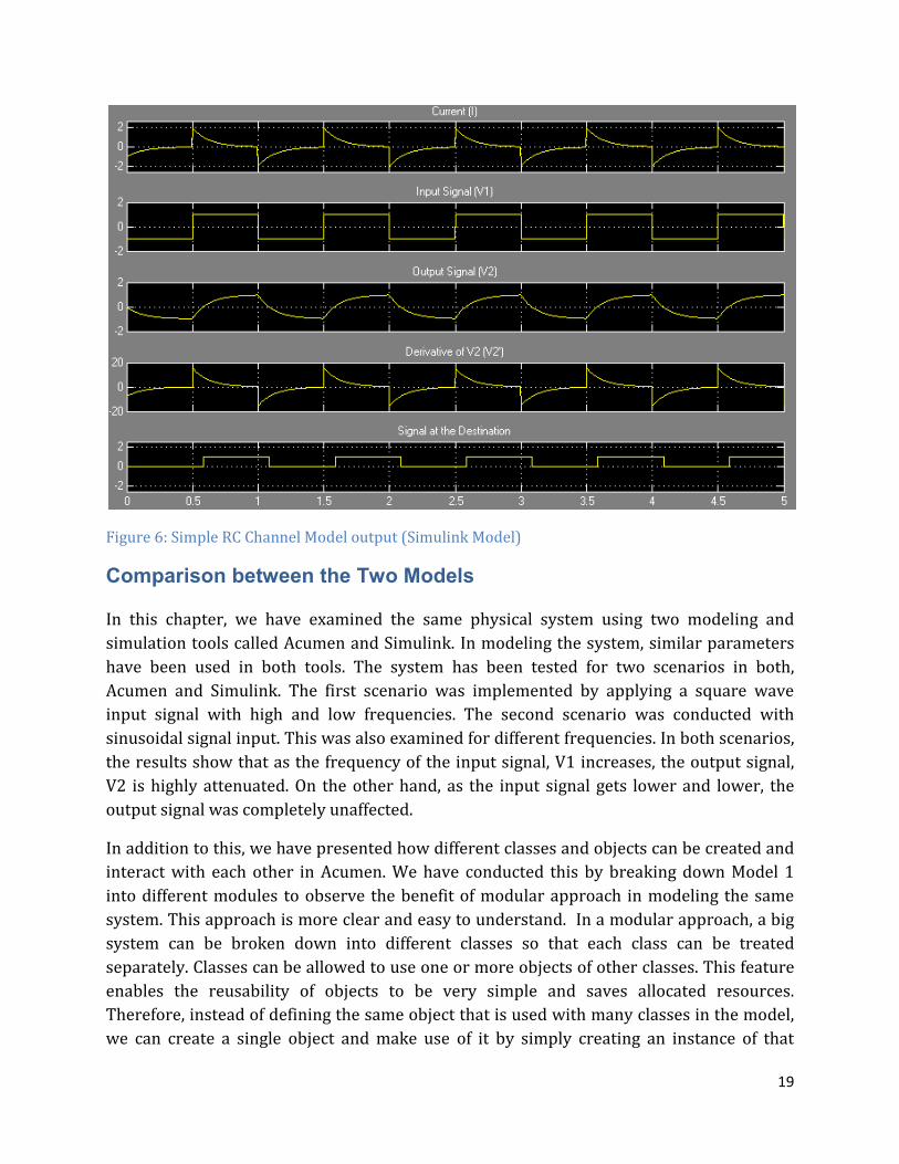
Figure 6: Simple RC Channel Model output (Simulink Model)

Comparison between the Two Models

In this chapter, we have examined the same physical system using two modeling and simulation tools called Acumen and Simulink. In modeling the system, similar parameters have been used in both tools. The system has been tested for two scenarios in both, Acumen and Simulink. The first scenario was implemented by applying a square wave input signal with high and low frequencies. The second scenario was conducted with sinusoidal signal input. This was also examined for different frequencies. In both scenarios, the results show that as the frequency of the input signal, V1 increases, the output signal, V2 is highly attenuated. On the other hand, as the input signal gets lower and lower, the output signal was completely unaffected.

In addition to this, we have presented how different classes and objects can be created and interact with each other in Acumen. We have conducted this by breaking down Model 1 into different modules to observe the benefit of modular approach in modeling the same system. This approach is more clear and easy to understand. In a modular approach, a big system can be broken down into different classes so that each class can be treated separately. Classes can be allowed to use one or more objects of other classes. This feature enables the reusability of objects to be very simple and saves allocated resources. Therefore, instead of defining the same object that is used with many classes in the model, we can create a single object and make use of it by simply creating an instance of that

20

object in a place where we need to use the object. This is one of the advantages of Acumen in the modeling process. The results found in both modular and non-modular approaches are identical in Acumen.

Simulink is a powerful popular tool for modeling and simulation of dynamical systems. In Simulink, it is very easy to build a model by simply using a drag-and-drop operation. This graphical representation makes the model and the algorithm easy to understand. However, when it comes to practical implementation and configuration of different block parameters, special care must be taken. We need to properly know how each block behaves and what parameters need to be configured. Otherwise, the model will achieve an undesired output. From the model presented, we found that in Acumen a very simple algorithm like natural language is used to generate the input signal. The whole Acumen code representing the system is very short and simple to understand. Similarly, Acumen allows direct use of the differential equation representing the physical system. However, in Simulink, this is not a straight forward operation.

When we compare the plots generated by Simulink with that of Acumen, Acumen plots the graph representing each variable automatically when we run the model. The interesting feature with Acumen generated plots is that we can read the value of any variable at any time t by simply dragging the mouse cursor on the graph of our interest. As all variables including constant variables are plotted automatically, Acumen does not allow users to plot only for the desired variables. This is the disadvantage in that it affects the actual view of the graphs when too many variables are used in the model. In Simulink, in order to plot a graph for the desired variable, we need to connect each variable to the Scope block. This shows that Simulink allows users to plot the graph of the desired variable.

The other important point to be noted here is that in Acumen all bands are normalized. This means that the height for each band is equal. Therefore, it is difficult for readers to visualize the change in height of the signal and the signal look as a whole. As opposed to this, when we look at the Simulink graphs, one can clearly see the variation of the graph as a result of different input signals.

In general, from the comparison made between Acumen and Simulink for the same model, we conclude that Acumen can be used to model an RC low-pass filter in a simple and easy to understand way.

21

Chapter 4: Amplitude Modulation

Introduction

Modulation is the process of varying one or more of the three fundamental frequency parameters called amplitude, frequency and phase. By modulation we mean encoding source information onto a high frequency power signal called a carrier signal. The message or modulating signal can be represented in different forms such as analog or digital. On the other hand, the carrier signal could be a sine wave, a cosine wave or a square wave. We consider a sine wave given by:

s�t� = A sin�2πft+ φ� (4.1)

In the carrier signal given in equation 4.1 above, the three parameters that can be modified are the amplitude (A), the frequency (f) and the phase (ϕ). Based on what we can modify, there are three basic types of Analog modulations called Amplitude modulation, Frequency modulation, and Phase modulation. This chapter presents an Amplitude modulation system. The AM system will be simulated using Acumen, MATLAB and Simulink. In amplitude modulation, the amplitude of the carrier signal is modulated (modified) in proportion to the baseband signal. In this modulation scheme, the frequency and phase are kept constant.

Amplitude Modulation and Demodulation

Amplitude modulation is the most well known modulation technique used with analog modulation in which the amplitude of the carrier signal is modulated, based on the message signal. Amplitude Modulation is formed by mixing the high frequency carrier signal with the message signal. Given a continuous sinusoidal carrier signal V(t)=Ac sin(2πfct) and modulating signal m(t), then the Amplitude Modulated signal s(t) is given by:

s�t� = Ac�C+ m�t�� sin�2πfct� (4.2)

Where Ac is a non-zero constant (amplitude), fc is the frequency of the carrier signals and C is a constant. C>|m(t)| must hold for all t.

Demodulation or detection is the process of regenerating the original base-band signal from the modulated signal. In other words, it is the reverse of the modulation process. Demodulation is performed at the AM receiver side. The two main methods of performing AM Demodulation are the coherent and non-coherent demodulations [7]. In the coherent demodulation (detection) method, the carrier signal (frequency and phase) is known at the

22

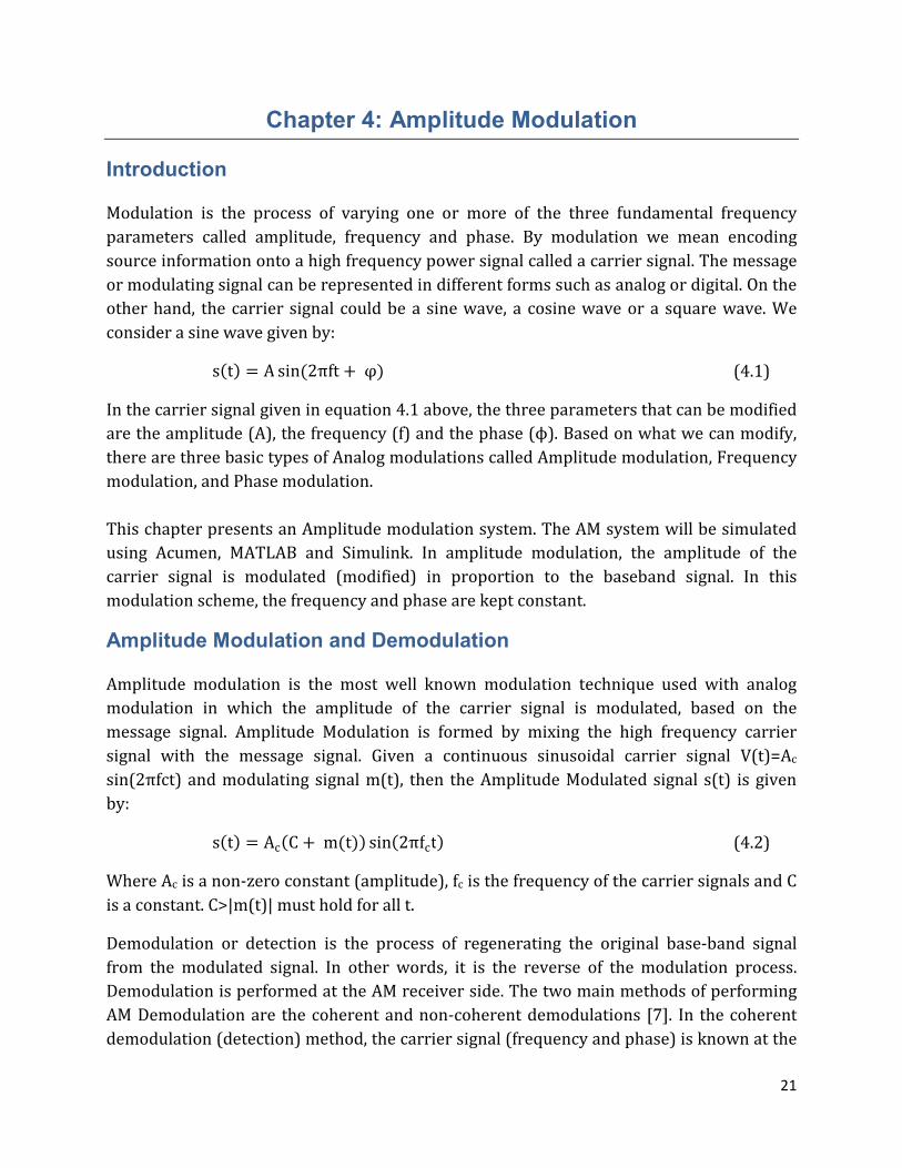
receiver. Thus, to demodulate the signal, the AM signal received from the transmitter is mixed (multiplied) with the carrier signal that was used in the modulation process and then followed by a low pass filter (LPF). Figure 7 below shows AM modulator and demodulator.

Figure 7: AM Modulator and Demodulator

In reality, coherent detection is relatively more complex and more expensive to achieve. Therefore, the other alternative called an envelope detector or Non-coherent Detection which is simple to implement with less performance can be used to demodulate an AM modulated signal. An envelope detector is a full-wave rectifier. In this chapter, an envelope detecttion (Non-coherent Detection) method will be used to model an AM system using Acumen, MATLAB and Simulink.

Acumen Model for Amplitude Modulation

The following model illustrates the process of modulation and demodulation of AM system. In this model, the signal is demodulated at the receiver with non-coherent detection method.

Model 3: Acumen Model for Amplitude Modulation

class Source()

private message = 0; pi=3.14159265; fm=1; Am=1; t=0; t'=0; end

t'[=]1;

message[=]Am*sin(2*pi*fm*t); //Message (Modulating) Signal

end

class Transmitter()

23

private carrier=0; input=0; am=0; t=0; t'=0; pi=3.14159265; Ac=1; fc=10; C=1.5; end

t'[=]1;

carrier[=]Ac*sin(2*pi*fc*t); //Carrier Signal

am[=]Ac*(C + input)*sin(2*3.14159265*fc*t); //Modulation

end

class Receiver()

private input=0; output=0; output'=0; RC=0.15; t=0; t'=0; r=0; q=0; carrier=0; end

t'[=]1;

r[=]abs(input); //Rectified signal

output'[=](r - output)/RC; //Demodulated signal

end

class Network()

private source = create Source(); transmitter = create Transmitter();

receiver = create Receiver(); end

transmitter.input[=]source.message; receiver.input[=]transmitter.am;

end

class Main (simulator)

private c = create Network() end

end

In the above model, a sinusoidal message is generated at the Source and sent to the transmitter. The transmitter uses the message signal to modulate the high frequency carrier signal to produce the AM signal. This is formed by simply mixing (multiplying) the carrier signal and message signals. When the AM signal is received by the receiver, it is first rectified by an envelope (diode) detector and then passed through a simple RC low-pass filter that produces the desired demodulated signal. The RC filter used in this model is exactly similar to the RC filter designed in the second chapter.

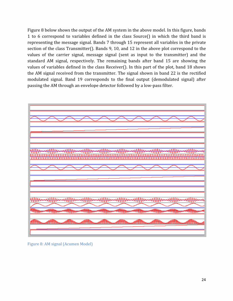
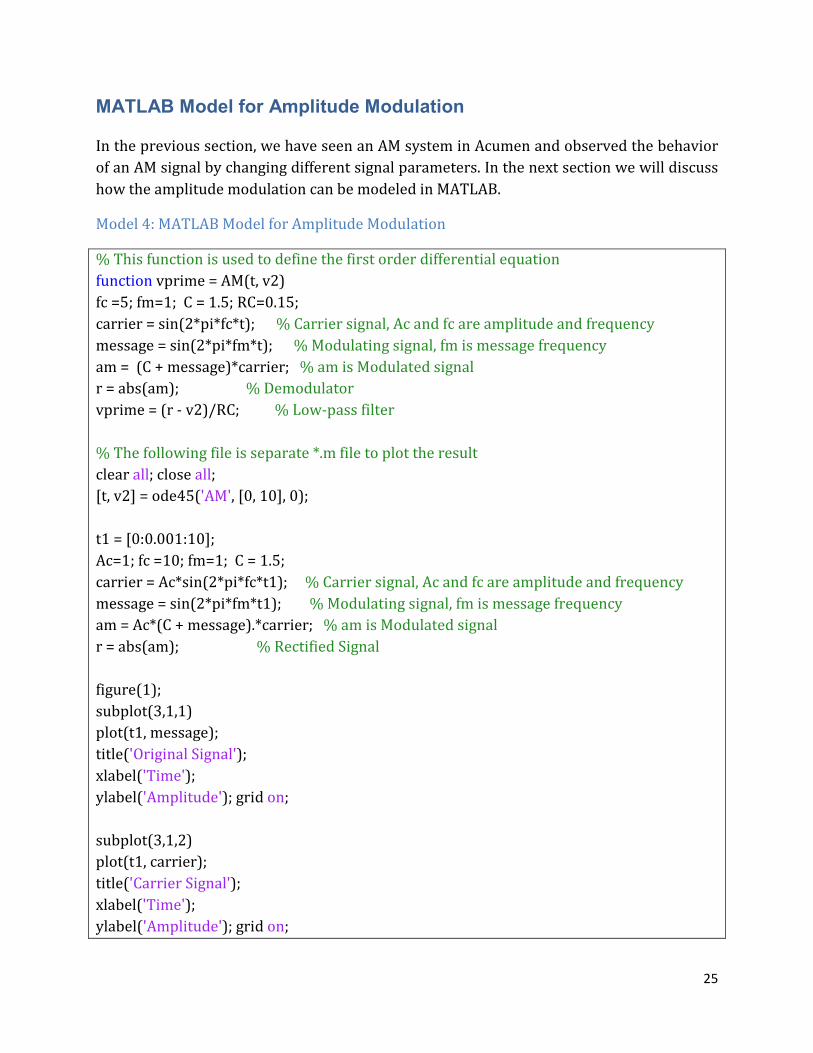
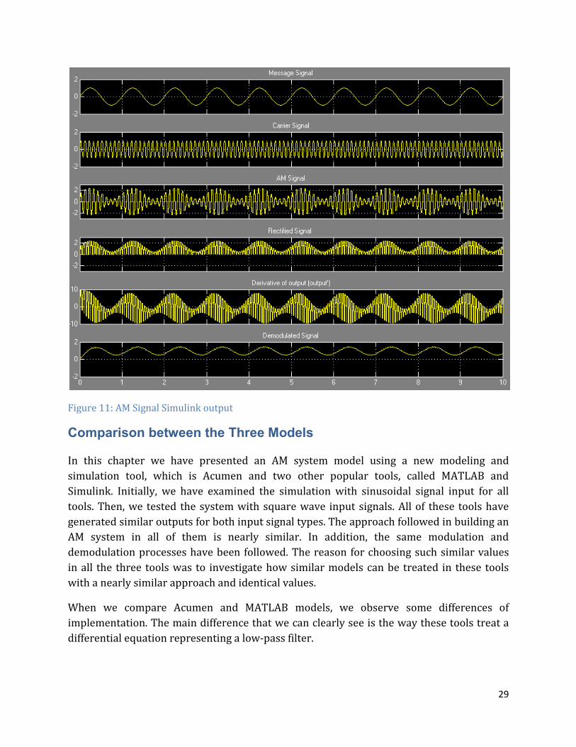
Figure 8 below shows the output of the AM system in the1 to 6 correspond to variables defined in the class Source() in which the third band is representing the message signal. Bands 7 through 15 represent all variables in the private section of the class Transmitter(). Bandsvalues of the carrier signal, message signal (sent as input to the transmitter) and the standard AM signal, respectively. The remaining bands after band 15 are showing the values of variables defined in ththe AM signal received from the transmitter. The signal shown in band 22 is the rectified modulated signal. Band 19 corresponds to the final output (demodulated signal) after passing the AM through an envelope detector followed by a low

Figure 8: AM signal (Acumen Model)

the output of the AM system in the above model. In this figure, bands 1 to 6 correspond to variables defined in the class Source() in which the third band is representing the message signal. Bands 7 through 15 represent all variables in the private section of the class Transmitter(). Bands 9, 10, and 12 in the above plot correspond to the values of the carrier signal, message signal (sent as input to the transmitter) and the standard AM signal, respectively. The remaining bands after band 15 are showing the values of variables defined in the class Receiver(). In this part of the plot, band 18 shows the AM signal received from the transmitter. The signal shown in band 22 is the rectified modulated signal. Band 19 corresponds to the final output (demodulated signal) after

h an envelope detector followed by a low-pass filter.

: AM signal (Acumen Model)

24

above model. In this figure, bands 1 to 6 correspond to variables defined in the class Source() in which the third band is representing the message signal. Bands 7 through 15 represent all variables in the private

9, 10, and 12 in the above plot correspond to the values of the carrier signal, message signal (sent as input to the transmitter) and the standard AM signal, respectively. The remaining bands after band 15 are showing the

e class Receiver(). In this part of the plot, band 18 shows the AM signal received from the transmitter. The signal shown in band 22 is the rectified modulated signal. Band 19 corresponds to the final output (demodulated signal) after

25

MATLAB Model for Amplitude Modulation

In the previous section, we have seen an AM system in Acumen and observed the behavior of an AM signal by changing different signal parameters. In the next section we will discuss how the amplitude modulation can be modeled in MATLAB.

Model 4: MATLAB Model for Amplitude Modulation

% This function is used to define the first order differential equation function vprime = AM(t, v2) fc =5; fm=1; C = 1.5; RC=0.15; carrier = sin(2*pi*fc*t); % Carrier signal, Ac and fc are amplitude and frequency message = sin(2*pi*fm*t); % Modulating signal, fm is message frequency am = (C + message)*carrier; % am is Modulated signal r = abs(am); % Demodulator vprime = (r - v2)/RC; % Low-pass filter % The following file is separate *.m file to plot the result clear all; close all; [t, v2] = ode45('AM', [0, 10], 0); t1 = [0:0.001:10]; Ac=1; fc =10; fm=1; C = 1.5; carrier = Ac*sin(2*pi*fc*t1); % Carrier signal, Ac and fc are amplitude and frequency message = sin(2*pi*fm*t1); % Modulating signal, fm is message frequency am = Ac*(C + message).*carrier; % am is Modulated signal r = abs(am); % Rectified Signal figure(1); subplot(3,1,1) plot(t1, message); title('Original Signal'); xlabel('Time'); ylabel('Amplitude'); grid on; subplot(3,1,2) plot(t1, carrier); title('Carrier Signal'); xlabel('Time'); ylabel('Amplitude'); grid on;

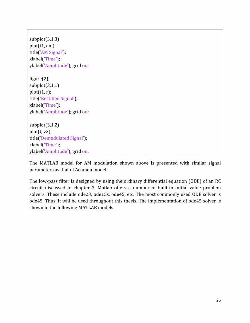
26

subplot(3,1,3) plot(t1, am); title('AM Signal'); xlabel('Time'); ylabel('Amplitude'); grid on; figure(2); subplot(3,1,1) plot(t1, r); title('Rectified Signal'); xlabel('Time'); ylabel('Amplitude'); grid on; subplot(3,1,2) plot(t, v2); title('Demodulated Signal'); xlabel('Time'); ylabel('Amplitude'); grid on;

The MATLAB model for AM modulation shown above is presented with similar signal parameters as that of Acumen model.

The low-pass filter is designed by using the ordinary differential equation (ODE) of an RC circuit discussed in chapter 3. Matlab offers a number of built-in initial value problem solvers. These include ode23, ode15s, ode45, etc. The most commonly used ODE solver is ode45. Thus, it will be used throughout this thesis. The implementation of ode45 solver is shown in the following MATLAB models.

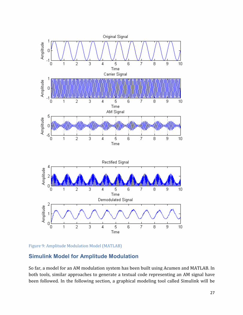
Figure 9: Amplitude Modulation Model

Simulink Model for Amplitude Modulation

So far, a model for an AM modulation both tools, similar approachesbeen followed. In the following section

Model (MATLAB)

Amplitude Modulation

an AM modulation system has been built using Acumen and es to generate a textual code representing an AM signal

In the following section, a graphical modeling tool called Simulink

27

using Acumen and MATLAB. In to generate a textual code representing an AM signal have

a graphical modeling tool called Simulink will be

28

used to model the same system that was implemented in Acumen and MATLAB in the previous sections. As we have discussed in the third chapter, the Simulink model is built with the help of different blocks from different libraries. The Amplitude modulation model is also developed in a similar way by dragging and dropping appropriate blocks into the model window. Figure 10 below illustrates the Simulink basic building block diagram of an AM system.

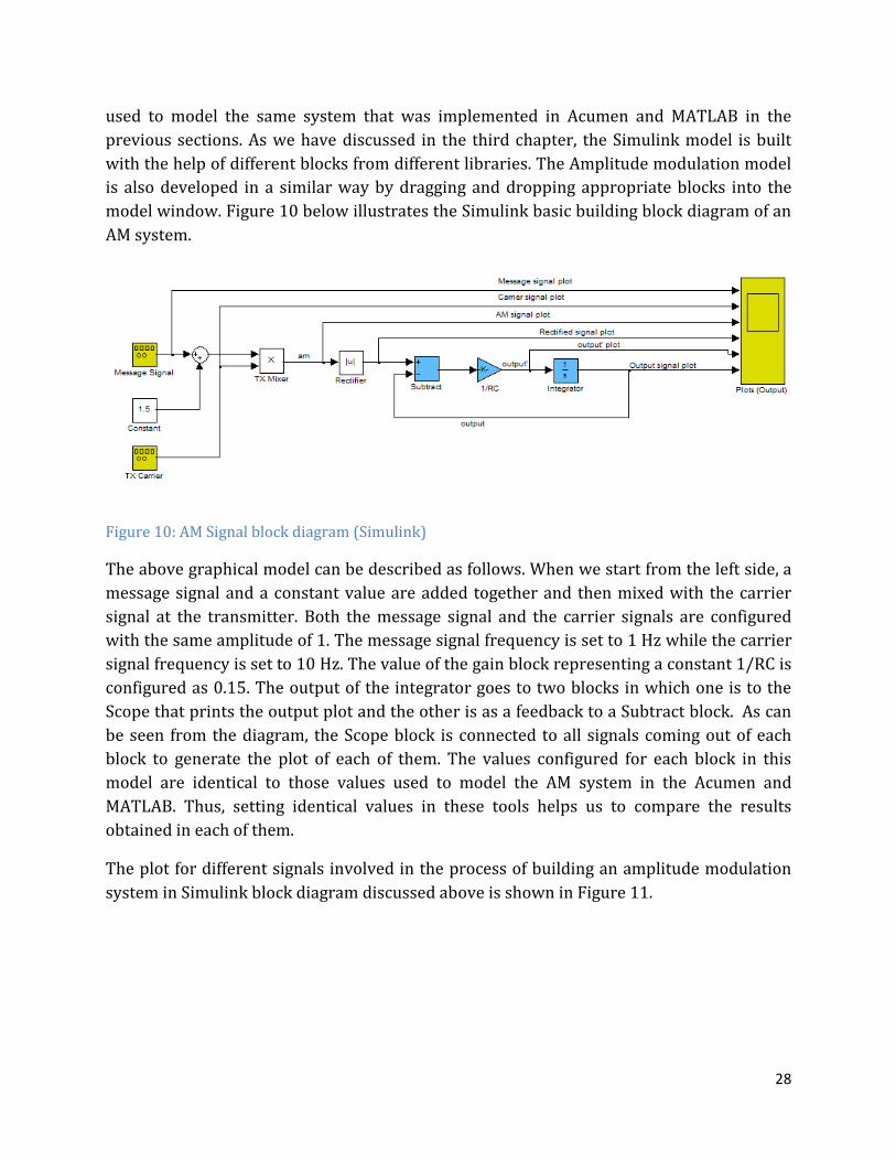
Figure 10: AM Signal block diagram (Simulink)

The above graphical model can be described as follows. When we start from the left side, a message signal and a constant value are added together and then mixed with the carrier signal at the transmitter. Both the message signal and the carrier signals are configured with the same amplitude of 1. The message signal frequency is set to 1 Hz while the carrier signal frequency is set to 10 Hz. The value of the gain block representing a constant 1/RC is configured as 0.15. The output of the integrator goes to two blocks in which one is to the Scope that prints the output plot and the other is as a feedback to a Subtract block. As can be seen from the diagram, the Scope block is connected to all signals coming out of each block to generate the plot of each of them. The values configured for each block in this model are identical to those values used to model the AM system in the Acumen and MATLAB. Thus, setting identical values in these tools helps us to compare the results obtained in each of them.

The plot for different signals involved in the process of building an amplitude modulation system in Simulink block diagram discussed above is shown in Figure 11.

29

Figure 11: AM Signal Simulink output

Comparison between the Three Models

In this chapter we have presented an AM system model using a new modeling and simulation tool, which is Acumen and two other popular tools, called MATLAB and Simulink. Initially, we have examined the simulation with sinusoidal signal input for all tools. Then, we tested the system with square wave input signals. All of these tools have generated similar outputs for both input signal types. The approach followed in building an AM system in all of them is nearly similar. In addition, the same modulation and demodulation processes have been followed. The reason for choosing such similar values in all the three tools was to investigate how similar models can be treated in these tools with a nearly similar approach and identical values.

When we compare Acumen and MATLAB models, we observe some differences of implementation. The main difference that we can clearly see is the way these tools treat a differential equation representing a low-pass filter.

30

In MATLAB, two MATLAB scripts have been used to perform the integration and simulate the low-pass filter. One script (file) is a derivative function that contains the ordinary differential equation to be solved. The other file is used to plot the results. In the derivative (solver) function, we need to define the parameters to be passed to the differential equation. In the later script that is used to plot the results, a built-in function called ode45 is called with this file. This adds extra tasks and complexity to solving differential equations. The other problem with this is that the function on the file to be used with the ODE functions must have only two arguments, t and output of the integrator [8]. This limits additional parameters required to describe the differential equation not to be passed to the function when it is called. In Acumen, the differential equation representing the low-pass filter is directly used in the model. This makes Acumen a very simple tool to work with ordinary differential equations.

On the other hand, when we compare the Acumen model with the graphical Simulink, we see similar outputs in both tools. The main difference we can observe is that in Acumen, we need to write a code for each object in the system. Simulink has got rich libraries in which many readymade blocks are used to model the system. If we know how to configure different parameters for each block in the system, it needs less energy and time to build the system as compared to Acumen and MATLAB. However, when compared to Acumen for more complex models Simulink needs more time to setup the complete system and configure it. In addition, the main problem of Simulink is that there is no clear semantics behind the manipulated diagrams [9].

31

Chapter 5: Angular Modulation

Introduction

In the previous chapter, we have discussed basic concepts about analog modulation techniques and the amplitude modulation and demodulation process. In this chapter, we will discuss the angular modulation technique which is the alternative to the AM. In angular modulation, the angle of the carrier signal is varied according to the amplitude of the message (modulating) signal. Angular modulation consists of the Frequency Modulation and Phase Modulation. The time domain representation of an angle modulated signal can be expressed as:

���� = A� cos�θi�t�� (5.1)

Phase Modulation (PM)

Phase modulation is a technique in which the phase of the carrier signal is varied in accordance with the message signal From equation 5.1, θi(t) is given by θi(t)= 2πfct + k(m(t)) for PM signal. k is phase sensitivity constant and 2πfct is the angle of the carrier signal. The modulating signal m(t), is used to determine the momentary phase [10]. Suppose we are given modulating signal m(t), then a phase modulated signal is:

���� = A� cos�2���� + km�t�� (5.2)

Frequency Modulation (FM)

In the FM modulation technique, the frequency of the carrier signal is modulated in proportion to the baseband signal. In other words, the frequency of a modulating signal is used to directly vary the frequency of a carrier signal. Bearing in mind that an angle modulated signal s(t) = Ac cos(θi(t)), then for FM signal θi(t) is given by θi(t)= 2πfc t + β ∫(m(t)dt. Then a Frequency modulated (FM) signal is given by:

���� = A� cos�2���� + !∫ m�t�dt� (5.3)

where m(t) is the modulating signal, Ac and fc are the carrier amplitude and frequency, respectively and β is a frequency modulation index. Depending on the value of β, FM can be

32

either narrowband or wideband. For a small value of β (β<<1), FM is known as Narrowband and for a large value of β (β ≈ 1), it is known as a Wideband.

Demodulation of PM and FM

From equation 5.2, we know that the PM modulated signal is:

���� = A� cos�2���� + km�t��

Then, this signal can be demodulated by finding the derivative of the modulated signal, s(t) [10]. The PM signal after differentiator produces a signal for which the amplitude depends on the modulating signal, m(t), but having a varying carrier phase. For PM demodulation, the differentiated signal is passed through an envelope detector followed by an Integrator to produce the desired output. Similarly, from equation 5.3 we know that the FM signal is given by:

���� = A� cos�2���� + !∫ m�t�dt�

Consequently, taking the derivative of s(t) produces a signal which is then passed through an envelope detector to produce the desired output [11]. Assuming that a message signal with a frequency of 1Hz, carrier frequency of 10 Hz and the constants β = 5 are used, we will now consider how Acumen can be used to model the frequency modulation system discussed above.

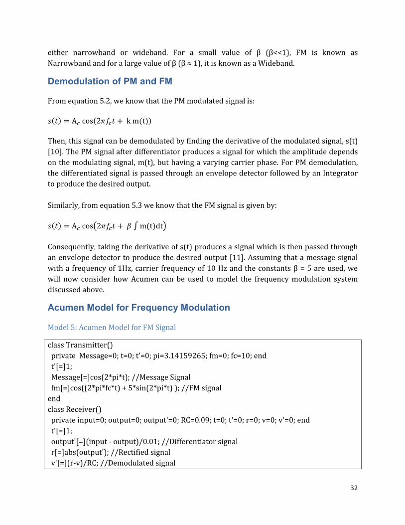
Acumen Model for Frequency Modulation

Model 5: Acumen Model for FM Signal

class Transmitter() private Message=0; t=0; t'=0; pi=3.14159265; fm=0; fc=10; end t'[=]1; Message[=]cos(2*pi*t); //Message Signal fm[=]cos((2*pi*fc*t) + 5*sin(2*pi*t) ); //FM signal end class Receiver() private input=0; output=0; output'=0; RC=0.09; t=0; t'=0; r=0; v=0; v'=0; end t'[=]1; output'[=](input - output)/0.01; //Differentiator signal r[=]abs(output'); //Rectified signal v'[=](r-v)/RC; //Demodulated signal

33

end class Network() private transmitter = create Transmitter(); receiver = create Receiver(); end receiver.input[=]transmitter.fm; end class Main (simulator) private c = create Network() end end

In the above model, a very simple and easily implemented Acumen code is used to build a model representing the modulation and demodulation of an FM signal. In the class Transmitter(), the FM signal is formed based on equation 5.3. In this process, the integral of the message signal is added to the carrier angle to alter the carrier signal. On the other hand, on the receiver side the modulated signal is differentiated and passed to envelope detector followed by a low-pass filter. Figure 12 shows the relationship between the message signal, carrier signal, modulated signal, and FM signal, after differentiator and the final output.

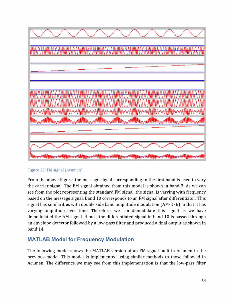
Figure 12: FM signal (Acumen)

From the above Figure, the message signal corresponding to the first band is used to vary the carrier signal. The FM signal obtained from this model is shown in band 3. As we can see from the plot representing the standard FM signal, the signal is varying based on the message signal. Band 10 corresponds to an FM signal after differentiator. This signal has similarities with double side band amplitude modulation (AMvarying amplitude over time. Therefore, we can demodulate demodulated the AM signal. Hence, the differentiated signal in band 10 is passed through an envelope detector followed by a lowband 14.

MATLAB Model for Frequency Modulation

The following model shows the previous model. This model is implemented using similar methods to those followed in Acumen. The difference we may see from this implementation is that the low

From the above Figure, the message signal corresponding to the first band is used to vary the carrier signal. The FM signal obtained from this model is shown in band 3. As we can see from the plot representing the standard FM signal, the signal is varying based on the message signal. Band 10 corresponds to an FM signal after differentiator. This signal has similarities with double side band amplitude modulation (AM-DSB) in that it has varying amplitude over time. Therefore, we can demodulate this signal as we have demodulated the AM signal. Hence, the differentiated signal in band 10 is passed through an envelope detector followed by a low-pass filter and produced a final output as shown in

Model for Frequency Modulation

The following model shows the MATLAB version of an FM signal built in Acumen in the previous model. This model is implemented using similar methods to those followed in Acumen. The difference we may see from this implementation is that the low

34

From the above Figure, the message signal corresponding to the first band is used to vary the carrier signal. The FM signal obtained from this model is shown in band 3. As we can see from the plot representing the standard FM signal, the signal is varying with frequency based on the message signal. Band 10 corresponds to an FM signal after differentiator. This

DSB) in that it has this signal as we have

demodulated the AM signal. Hence, the differentiated signal in band 10 is passed through pass filter and produced a final output as shown in

version of an FM signal built in Acumen in the previous model. This model is implemented using similar methods to those followed in Acumen. The difference we may see from this implementation is that the low-pass filter

35

used in this version is different from the filter used in Acumen. In this model a built-in filter called Butterworth is used

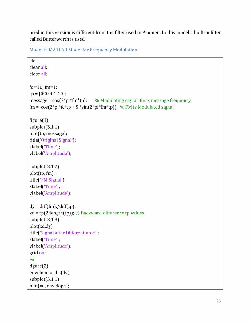
Model 6: MATLAB Model for Frequency Modulation

clc clear all; close all; fc =10; fm=1; tp = [0:0.001:10]; message = cos(2*pi*fm*tp); % Modulating signal, fm is message frequency fm = cos(2*pi*fc*tp + 5.*sin(2*pi*fm*tp)); % FM is Modulated signal figure(1); subplot(3,1,1) plot(tp, message); title('Original Signal'); xlabel('Time'); ylabel('Amplitude'); subplot(3,1,2) plot(tp, fm); title('FM Signal'); xlabel('Time'); ylabel('Amplitude'); dy = diff(fm)./diff(tp); xd = tp(2:length(tp)); % Backward difference tp values subplot(3,1,3) plot(xd,dy) title('Signal after Differentiator'); xlabel('Time'); ylabel('Amplitude'); grid on; % figure(2); envelope = abs(dy); subplot(3,1,1) plot(xd, envelope);

title('Rectified Signal'); xlabel('Time'); ylabel('Amplitude'); grid on; % Low Pass filter cutoff_f = 6; fs=1000;% cutoff frequency k = cutoff_f/(fs/2); % normalized cut off frequency [b1,a1] = butter(2,k, 'low'); % Butterworth Low pass filter output = filtfilt(b1,a1,envelope); subplot(3,1,2) plot(xd, output); title('Demodulated Signal'); xlabel('Time'); ylabel('Amplitude'); grid on;

% cutoff frequency % normalized cut off frequency

% Butterworth Low pass filter output = filtfilt(b1,a1,envelope); % Filtered signal

36

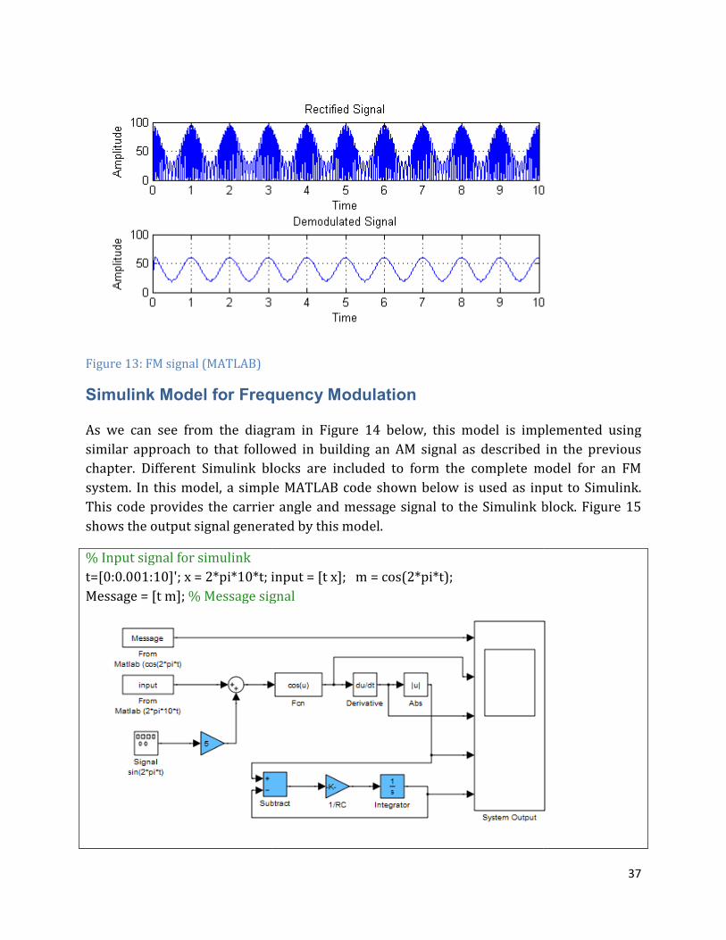
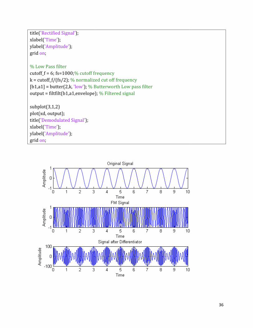
Figure 13: FM signal (MATLAB)

Simulink Model for Frequency Modulation

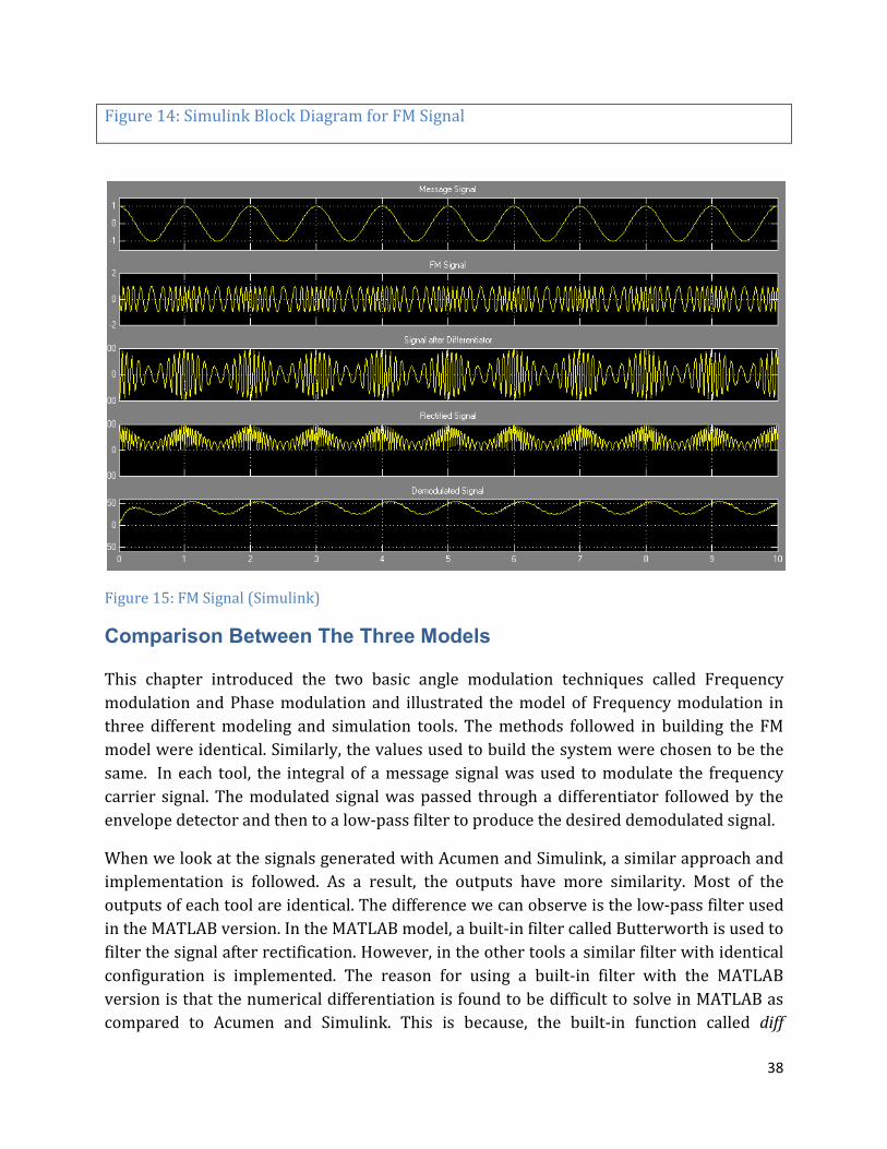
As we can see from the diagram in Figure 14 below, this model is implemented using similar approach to that followed in building an AM signal as described in the previous chapter. Different Simulink blocks are included to form the complete model for an FM system. In this model, a simple This code provides the carrier angle and message signal to the Simulink block. shows the output signal generated by this model

% Input signal for simulink t=[0:0.001:10]'; x = 2*pi*10*t; input = [t x]; Message = [t m]; % Message signal

Simulink Model for Frequency Modulation

As we can see from the diagram in Figure 14 below, this model is implemented using similar approach to that followed in building an AM signal as described in the previous chapter. Different Simulink blocks are included to form the complete model for an FM system. In this model, a simple MATLAB code shown below is used as input to Simulink. This code provides the carrier angle and message signal to the Simulink block. shows the output signal generated by this model.

input = [t x]; m = cos(2*pi*t); % Message signal

37

As we can see from the diagram in Figure 14 below, this model is implemented using similar approach to that followed in building an AM signal as described in the previous chapter. Different Simulink blocks are included to form the complete model for an FM

code shown below is used as input to Simulink. This code provides the carrier angle and message signal to the Simulink block. Figure 15

38

Figure 14: Simulink Block Diagram for FM Signal

Figure 15: FM Signal (Simulink)

Comparison Between The Three Models

This chapter introduced the two basic angle modulation techniques called Frequency modulation and Phase modulation and illustrated the model of Frequency modulation in three different modeling and simulation tools. The methods followed in building the FM model were identical. Similarly, the values used to build the system were chosen to be the same. In each tool, the integral of a message signal was used to modulate the frequency carrier signal. The modulated signal was passed through a differentiator followed by the envelope detector and then to a low-pass filter to produce the desired demodulated signal.

When we look at the signals generated with Acumen and Simulink, a similar approach and implementation is followed. As a result, the outputs have more similarity. Most of the outputs of each tool are identical. The difference we can observe is the low-pass filter used in the MATLAB version. In the MATLAB model, a built-in filter called Butterworth is used to filter the signal after rectification. However, in the other tools a similar filter with identical configuration is implemented. The reason for using a built-in filter with the MATLAB version is that the numerical differentiation is found to be difficult to solve in MATLAB as compared to Acumen and Simulink. This is because, the built-in function called diff

39

computes differences between elements in an array [12]. However, the function that solves the ODE provides scalar values. As the filters used in MATLAB differs from a filter used with Acumen and Simulink, the final output (demodulated signal) of the FM system in MATLAB shows some differences from the output generated by the other tools.

40

Chapter 6: Binary Amplitude Shift Keying

Digital Modulation Techniques

The modulation process in digital communication corresponds to switching the amplitude, frequency or phase angle of the carrier signal in accordance with the modulating (message) signal. Depending on the parameter(s) used to alter the carrier frequency, there are three basic digital modulation techniques called amplitude shift keying, frequency shift keying and phase shift keying [13]. In this chapter, we will consider the basic binary digital modulation called a binary Amplitude Shift Keying.

Binary Amplitude Shift Keying (BASK)

In the BASK modulation technique, the digital data is represented by varying the amplitude of a carrier signal. The carrier signal strength is varied to represent binary 0 or 1 in accordance with the message signal. ASK is often known as on-off keying (OOK). In this modulation technique, the frequency and phase of the carrier signal are kept constant. Mathematically, Binary ASK, s(t) can be defined as:

s�t� = $A% sin�2πf%t� , binary10,binary0. (6.1)

Where Ac is a constant Amplitude and fc is the carrier frequency. The following model represents the BASK signal in Acumen. BASK signal is generated by mixing the message signal with the carrier signal. This is what the following model tries to produce. The model consists of different classes representing signal source, a transmitter, a receiver and destination. In the approach followed in the model, the signal generated by the source is sent as input to the transmitter which modulates the signal received from the source and then sends its output to the receiver through a given channel. The receiver which demodulates the signal received from the transmitter then passes over the output to the destination. The destination in its turn uses a given threshold to decide whether 0 or 1 was transmitted. In this hierarchical approach, the class called Network(), creates an instance of all other classes and links them together so that one class can use the objects of the other classes. Finally, the class Main(), creates an instance of the linking class, Network() and executes the whole model. The classes are represented in the graph in the order they are created in the class called Network() in this model. This feature of Acumen avoids the mixing up of variables from different classes and keeps the variables defined in the same class to be plotted under a similar class.

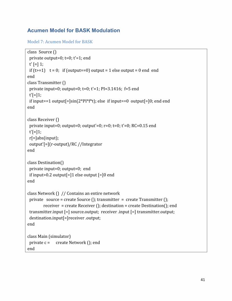
41

Acumen Model for BASK Modulation

Model 7: Acumen Model for BASK

class Source () private output=0; t=0; t'=1; end t' [=] 1; if (t>=1) t = 0; if (output==0) output = 1 else output = 0 end end end class Transmitter () private input=0; output=0; t=0; t'=1; PI=3.1416; f=5 end t'[=]1; if input==1 output[=]sin(2*PI*f*t); else if input==0 output[=]0; end end end class Receiver () private input=0; output=0; output'=0; r=0; t=0; t'=0; RC=0.15 end t'[=]1; r[=]abs(input); output'[=](r-output)/RC //Integrator end class Destination() private input=0; output=0; end if input>0.2 output[=]1 else output [=]0 end end class Network () // Contains an entire network private source = create Source (); transmitter = create Transmitter (); receiver = create Receiver (); destination = create Destination(); end transmitter.input [=] source.output; receiver .input [=] transmitter.output; destination.input[=]receiver .output; end class Main (simulator) private c = create Network (); end end

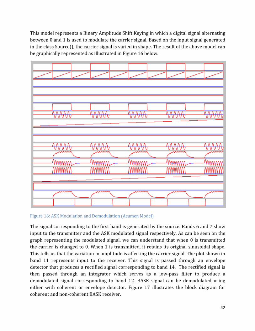
This model represents a Binary Amplitude Shift Keying in which a digital signal alternating between 0 and 1 is used to modulate the carrier signal. Based on the input signal generated in the class Source(), the carrier signal is varied in shape. The resultbe graphically represented as illustrated in Figure 16 below

Figure 16: ASK Modulation and Demodulation (Acumen Model)

The signal corresponding to the first band is generated by the source. Bands 6 and 7 input to the transmitter and the ASK modulated signal respectively. As can be seen on the graph representing the modulated signal, we can understand that when 0 is transmitted the carrier is changed to 0. When 1 is transmitted, it retains its originalThis tells us that the variation in amplitude is affecting the carrier signal. The plot shown in band 11 represents input to the receiverdetector that produces a rectified signal corresponding then passed through an integrator which serves as a lowdemodulated signal corresponding to band 12. either with coherent or envelope detector. Figure 17 illcoherent and non-coherent BASK receiver

This model represents a Binary Amplitude Shift Keying in which a digital signal alternating between 0 and 1 is used to modulate the carrier signal. Based on the input signal generated in the class Source(), the carrier signal is varied in shape. The result of the above model can be graphically represented as illustrated in Figure 16 below.

: ASK Modulation and Demodulation (Acumen Model)

The signal corresponding to the first band is generated by the source. Bands 6 and 7 input to the transmitter and the ASK modulated signal respectively. As can be seen on the graph representing the modulated signal, we can understand that when 0 is transmitted the carrier is changed to 0. When 1 is transmitted, it retains its original sinusoidal shape. This tells us that the variation in amplitude is affecting the carrier signal. The plot shown in band 11 represents input to the receiver. This signal is passed through an envelope

produces a rectified signal corresponding to band 14. The rectified signal is then passed through an integrator which serves as a low-pass filter to produce a demodulated signal corresponding to band 12. BASK signal can be demodulated using either with coherent or envelope detector. Figure 17 illustrates the block diagram for

BASK receiver.

42

This model represents a Binary Amplitude Shift Keying in which a digital signal alternating between 0 and 1 is used to modulate the carrier signal. Based on the input signal generated

of the above model can

The signal corresponding to the first band is generated by the source. Bands 6 and 7 show input to the transmitter and the ASK modulated signal respectively. As can be seen on the graph representing the modulated signal, we can understand that when 0 is transmitted

sinusoidal shape. This tells us that the variation in amplitude is affecting the carrier signal. The plot shown in

. This signal is passed through an envelope The rectified signal is

pass filter to produce a BASK signal can be demodulated using

ustrates the block diagram for

43

Finally, based on the value of a threshold, input (0.2 in this case), the destination (decision making device) decides whether the symbol 0 or 1 was transmitted. This means that if the threshold is greater than 0.2, then the decision making device (destination) determines that 1 was transmitted. On the other hand, if the threshold is less than 0.2, then the destination device determines that 0 was transmitted. The final output that is detected by the destination is represented in the last band of the above plot.

Figure 17: ASK receiver

MATLAB Model for BASK Modulator and Demodulator

The following model shows the MATLAB implementation of Binary Amplitude Shift Keying. In this model, a similar approach of producing AM modulated signal is followed. MATLAB has a built-in square wave that oscillates between -1 and +1 by default. The built-in square wave has a pulse width of 0.5. However, a square wave generated in the Acumen model above is oscillating between 0 and +1 with pulse width of 1. To make a square wave used in MATLAB similar to that of Acumen, we have generated a MATLAB code that plots a square wave similar to Acumen. The following model illustrates how a Binary Amplitude Shift Keying is built in MATLAB Model 8: MATLAB Model for BASK

% ODE Solver function function m = BASK(t, z) c=1; i=length(t); for j=1:1:i % Square wave period=2; a=mod(t(i),period); if (a<=period/2) V1=0; else V1 = 1; end if (V1 ==1)

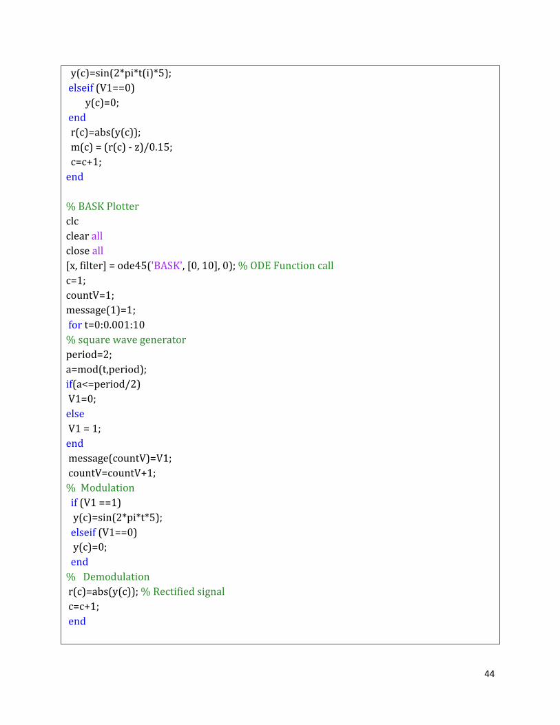
44

y(c)=sin(2*pi*t(i)*5); elseif (V1==0) y(c)=0; end r(c)=abs(y(c)); m(c) = (r(c) - z)/0.15; c=c+1; end % BASK Plotter clc clear all close all [x, filter] = ode45('BASK', [0, 10], 0); % ODE Function call c=1; countV=1; message(1)=1; for t=0:0.001:10 % square wave generator period=2; a=mod(t,period); if(a<=period/2) V1=0; else V1 = 1; end message(countV)=V1; countV=countV+1; % Modulation if (V1 ==1) y(c)=sin(2*pi*t*5); elseif (V1==0) y(c)=0; end % Demodulation r(c)=abs(y(c)); % Rectified signal c=c+1; end

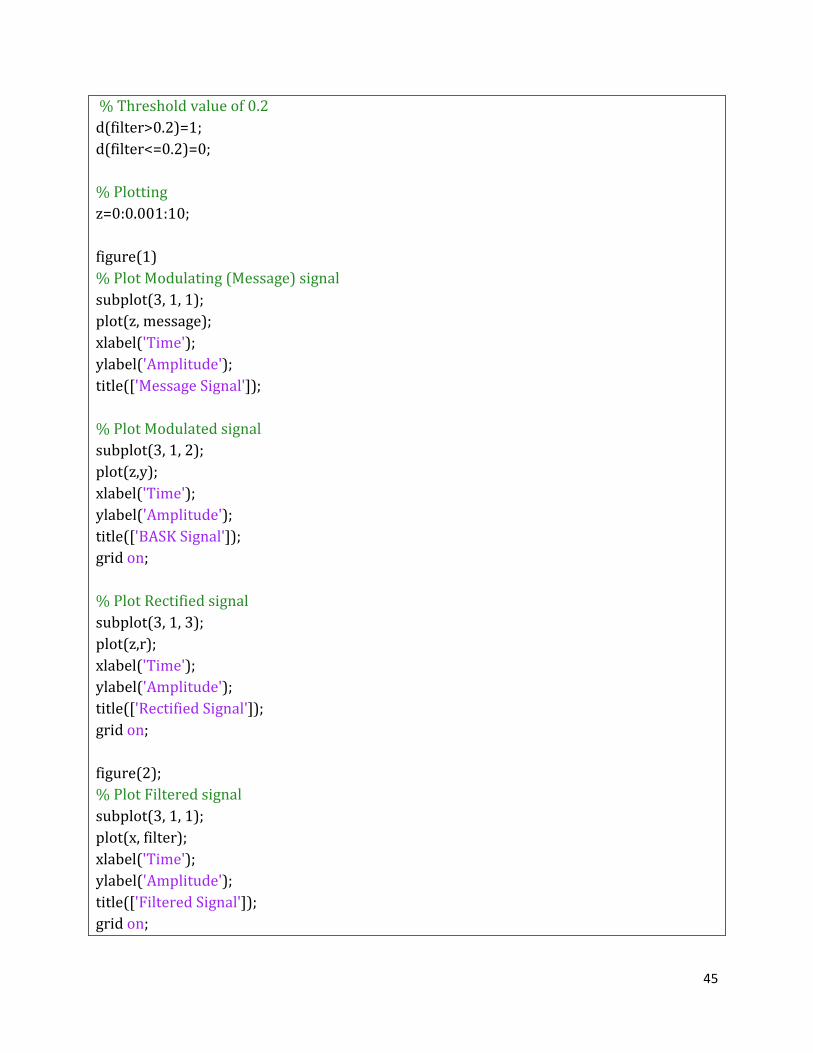
45

% Threshold value of 0.2 d(filter>0.2)=1; d(filter<=0.2)=0; % Plotting z=0:0.001:10; figure(1) % Plot Modulating (Message) signal subplot(3, 1, 1); plot(z, message); xlabel('Time'); ylabel('Amplitude'); title(['Message Signal']); % Plot Modulated signal subplot(3, 1, 2); plot(z,y); xlabel('Time'); ylabel('Amplitude'); title(['BASK Signal']); grid on; % Plot Rectified signal subplot(3, 1, 3); plot(z,r); xlabel('Time'); ylabel('Amplitude'); title(['Rectified Signal']); grid on; figure(2); % Plot Filtered signal subplot(3, 1, 1); plot(x, filter); xlabel('Time'); ylabel('Amplitude'); title(['Filtered Signal']); grid on;

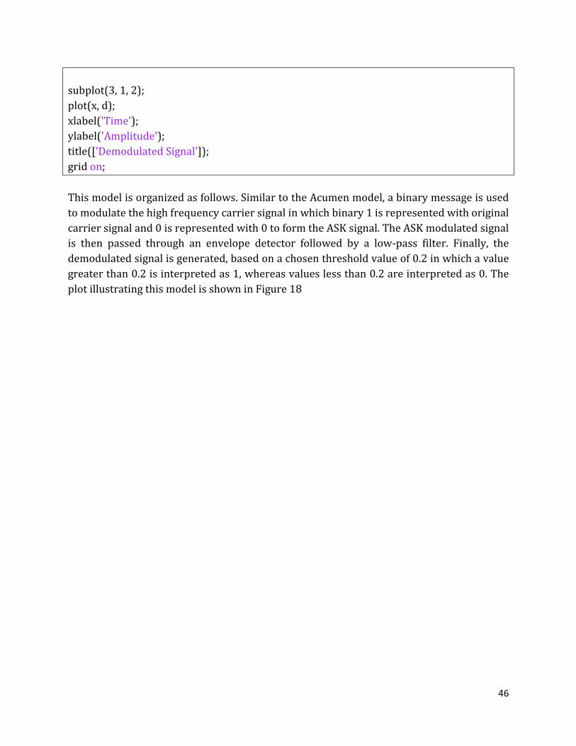
46

subplot(3, 1, 2); plot(x, d); xlabel('Time'); ylabel('Amplitude'); title(['Demodulated Signal']); grid on;

This model is organized as follows. Similar to the Acumen model, a binary message is used to modulate the high frequency carrier signal in which binary 1 is represented with original carrier signal and 0 is represented with 0 to form the ASK signal. The ASK modulated signal is then passed through an envelope detector followed by a low-pass filter. Finally, the demodulated signal is generated, based on a chosen threshold value of 0.2 in which a value greater than 0.2 is interpreted as 1, whereas values less than 0.2 are interpreted as 0. The plot illustrating this model is shown in Figure 18

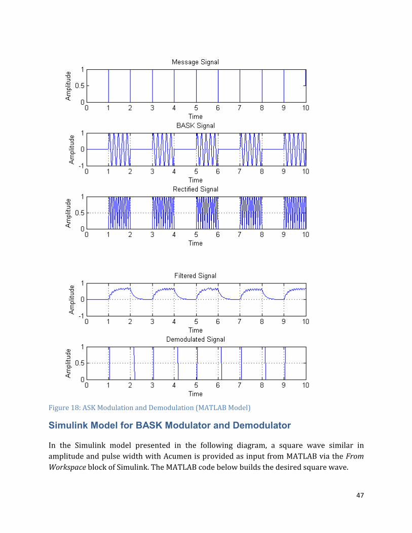
Figure 18: ASK Modulation and Demodulation (MATLAB Model)

Simulink Model for BASK Modulator and Demodulator

In the Simulink model presented in the following diagram, a square wave similar in amplitude and pulse width with Acumen is provided as input from Workspace block of Simulink. The

: ASK Modulation and Demodulation (MATLAB Model)

Simulink Model for BASK Modulator and Demodulator

presented in the following diagram, a square wave similar in amplitude and pulse width with Acumen is provided as input from MATLAB

The MATLAB code below builds the desired square wave

47

presented in the following diagram, a square wave similar in MATLAB via the From

code below builds the desired square wave.

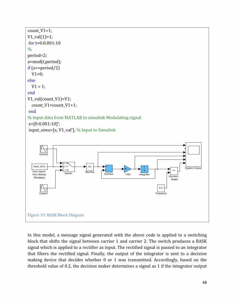
48

count_V1=1; V1_val(1)=1; for t=0:0.001:10 % period=2; a=mod(t,period); if (a<=period/2) V1=0; else V1 = 1; end V1_val(count_V1)=V1; count_V1=count_V1+1; end % Input data from MATLAB to simulink Modulating signal x=[0:0.001:10]'; input_simu=[x, V1_val']; % Input to Simulink

Figure 19: BASK Block Diagram

In this model, a message signal generated with the above code is applied to a switching block that shifts the signal between carrier 1 and carrier 2. The switch produces a BASK signal which is applied to a rectifier as input. The rectified signal is passed to an integrator that filters the rectified signal. Finally, the output of the integrator is sent to a decision making device that decides whether 0 or 1 was transmitted. Accordingly, based on the threshold value of 0.2, the decision maker determines a signal as 1 if the integrator output

0.2

Threshold

System Output >=

Switch Subtract

|u|

Rectifier

1

s

Integrator

input_simu

Input signal

from Matlab

(Message)

>=

Decision

Maker

Carrier2

Carrier1

-K-

1/RC

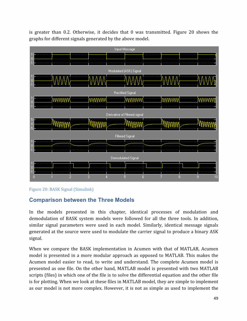
49

is greater than 0.2. Otherwise, it decides that 0 was transmitted. Figure 20 shows the graphs for different signals generated by the above model.

Figure 20: BASK Signal (Simulink)

Comparison between the Three Models

In the models presented in this chapter, identical processes of modulation and demodulation of BASK system models were followed for all the three tools. In addition, similar signal parameters were used in each model. Similarly, identical message signals generated at the source were used to modulate the carrier signal to produce a binary ASK signal.

When we compare the BASK implementation in Acumen with that of MATLAB, Acumen model is presented in a more modular approach as opposed to MATLAB. This makes the Acumen model easier to read, to write and understand. The complete Acumen model is presented as one file. On the other hand, MATLAB model is presented with two MATLAB scripts (files) in which one of the file is to solve the differential equation and the other file is for plotting. When we look at these files in MATLAB model, they are simple to implement as our model is not more complex. However, it is not as simple as used to implement the

50

BASK model covered in this chapter. In both Acumen and MATLAB, a similar method of filtering an AM signal covered in chapter 4 is followed to filter the rectified signal at the ASK receiver. As mentioned in chapter 4, the MATLAB model is using two MATLAB scripts (functions) to build the low-pass filter. Acumen implementation of the low-pass filter design differs from the MATLAB implementation in that a very simple code is used to represent the system. The reason for this is that Acumen allows direct use of the differential equation representing the low-pass filter. This reduces complexity of the code and makes the model easy to understand.

The comparison between Acumen and Simulink is identical to what has been discussed in the previous chapters while comparing these tools.

The results show that the plots generated by these tools are nearly identical. Finally, we can conclude in this chapter that Acumen can be used to build a model of similar type, with a simple approach.

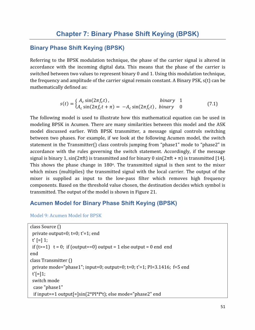
51

Chapter 7: Binary Phase Shift Keying (BPSK)

Binary Phase Shift Keying (BPSK)

Referring to the BPSK modulation technique, the phase of the carrier signal is altered in accordance with the incoming digital data. This means that the phase of the carrier is switched between two values to represent binary 0 and 1. Using this modulation technique, the frequency and amplitude of the carrier signal remain constant. A Binary PSK, s(t) can be mathematically defined as:

���� = $ /� sin�2����� ,01��231/� sin�2���� + �� = −/� sin�2����� , 01��230. (7.1)

The following model is used to illustrate how this mathematical equation can be used in modeling BPSK in Acumen. There are many similarities between this model and the ASK model discussed earlier. With BPSK transmitter, a message signal controls switching between two phases. For example, if we look at the following Acumen model, the switch statement in the Transmitter() class controls jumping from “phase1” mode to “phase2” in accordance with the rules governing the switch statement. Accordingly, if the message signal is binary 1, sin(2πft) is transmitted and for binary 0 sin(2πft + π) is transmitted [14]. This shows the phase change in 180o. The transmitted signal is then sent to the mixer which mixes (multiplies) the transmitted signal with the local carrier. The output of the mixer is supplied as input to the low-pass filter which removes high frequency components. Based on the threshold value chosen, the destination decides which symbol is transmitted. The output of the model is shown in Figure 21.

Acumen Model for Binary Phase Shift Keying (BPSK)

Model 9: Acumen Model for BPSK

class Source () private output=0; t=0; t'=1; end t' [=] 1; if (t>=1) t = 0; if (output==0) output = 1 else output = 0 end end end class Transmitter () private mode="phase1"; input=0; output=0; t=0; t'=1; PI=3.1416; f=5 end t'[=]1; switch mode case "phase1" if input==1 output[=]sin(2*PI*f*t); else mode="phase2" end

52

case "phase2" if input==0 output[=]sin(2*PI*f*t + PI); else mode="phase1" end end end class Receiver () private RC=0.15; r=0; f=5; input=0; output=0; output'=0; t=0; t'=0; PI=3.1416; end t'[=]1; r[=]sin(2*PI*f*t)*(input); //Rectified signal output'[=](r-output)/RC; //lowpass filter end class Destination() private input=0; output=0; end if input>0.026 output [=]1 else output [=]0 end //Destination end class Network () // Contains an entire network private source = create Source (); transmitter = create Transmitter (); receiver = create Receiver (); destination = create Destination(); end transmitter .input [=] source.output; receiver.input [=]transmitter .output; destination.input[=]receiver.output; end class Main (simulator) private c = create Network (); end end

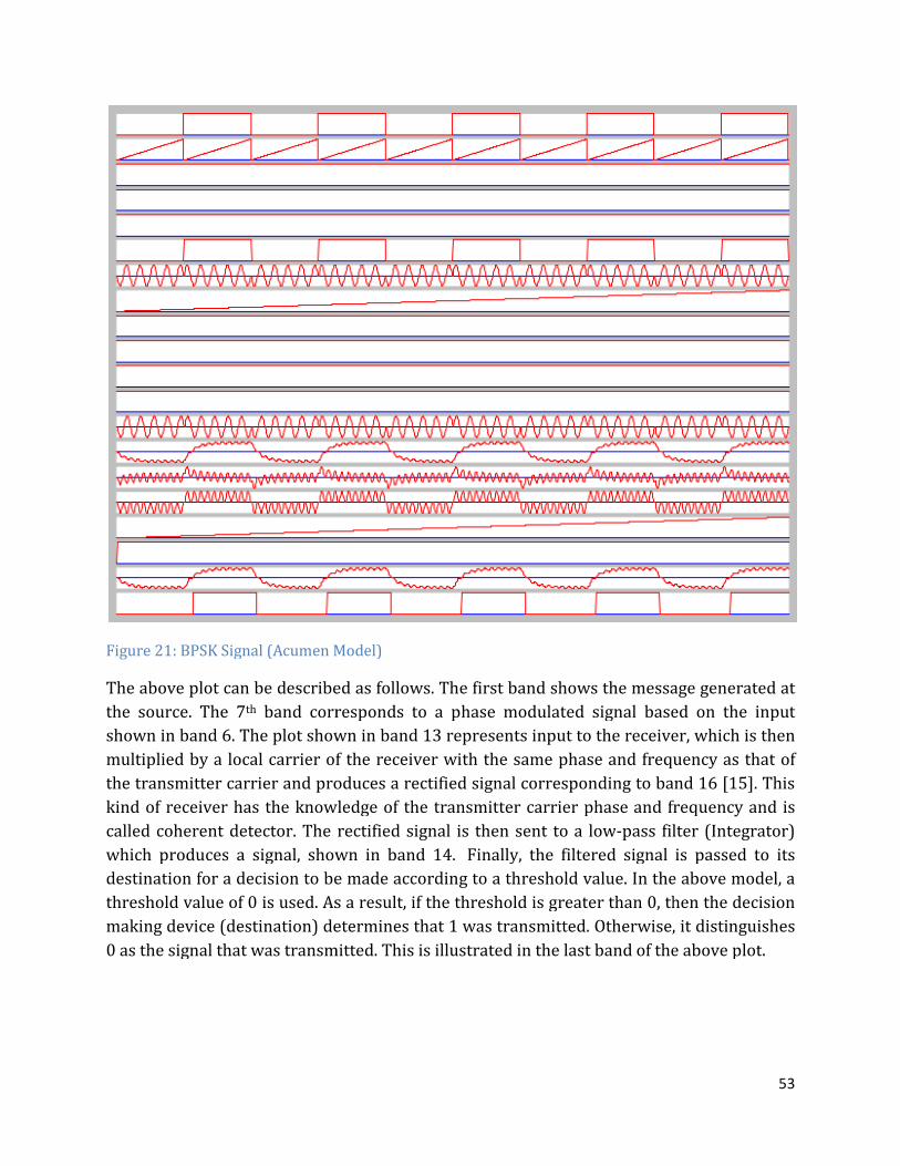
Figure 21: BPSK Signal (Acumen Model)

The above plot can be described as follows. The first band shows thethe source. The 7th band corresponds to a phase modulated signal based on the input shown in band 6. The plot shown in band 13 represents input to the receiver, which is then multiplied by a local carrier of the receiver with the samethe transmitter carrier and produces a rectified sigkind of receiver has the knowledge of the transmitter carrier phase and frequencalled coherent detector. The rectified signal is then sent to a lowwhich produces a signal, shown in band 14. destination for a decision to be made according to a thresholdthreshold value of 0 is used. As a result, if the threshold is greater than 0, then the decision making device (destination) determines that 1 was transmitted. Otherwise, it distinguishes 0 as the signal that was transmitted.

: BPSK Signal (Acumen Model)

The above plot can be described as follows. The first band shows the message generated at band corresponds to a phase modulated signal based on the input

shown in band 6. The plot shown in band 13 represents input to the receiver, which is then multiplied by a local carrier of the receiver with the same phase and frequency as that of the transmitter carrier and produces a rectified signal corresponding to band 16 kind of receiver has the knowledge of the transmitter carrier phase and frequencalled coherent detector. The rectified signal is then sent to a low-pass filter (Integrator) which produces a signal, shown in band 14. Finally, the filtered signal is passed to its destination for a decision to be made according to a threshold value. In the above model, a threshold value of 0 is used. As a result, if the threshold is greater than 0, then the decision making device (destination) determines that 1 was transmitted. Otherwise, it distinguishes 0 as the signal that was transmitted. This is illustrated in the last band of the above plot

53

message generated at band corresponds to a phase modulated signal based on the input

shown in band 6. The plot shown in band 13 represents input to the receiver, which is then phase and frequency as that of

nal corresponding to band 16 [15]. This kind of receiver has the knowledge of the transmitter carrier phase and frequency and is

pass filter (Integrator) Finally, the filtered signal is passed to its

value. In the above model, a threshold value of 0 is used. As a result, if the threshold is greater than 0, then the decision making device (destination) determines that 1 was transmitted. Otherwise, it distinguishes

This is illustrated in the last band of the above plot.

54

MATLAB Model for Binary Phase Shift Keying (BPSK)

Having understood how Acumen is used to model BASK, now let us consider the MATLAB implementation of the same model. Similar to the Acumen model discussed earlier for BPSK system, a digital message is used to control switching between carrier signals 1 and 2 [16]. This is illustrated in the following model.

Model 10: MATLAB Model for BPSK

% ODE solver function function m = BPSK(t, z) c=1; i=length(t); for j=1:1:i % period=2; a=mod(t(i),period); if (a<=period/2) V1=0; else V1 = 1; end if (V1 ==1) y(c)=sin(2*pi*t(i)*5); elseif (V1==0) y(c)=-sin(2*pi*t(i)*5); end r(c)=sin(2*pi*t(i)*5).*(y(c)); m(c) = (r(c) - z)/0.15; c=c+1; end % BPSK plotter [x, filter] = ode45('BPSK', [0, 10], 0); c=1; countV=1; message(1)=1; for t=0:0.001:10 % square wave generator period=2;

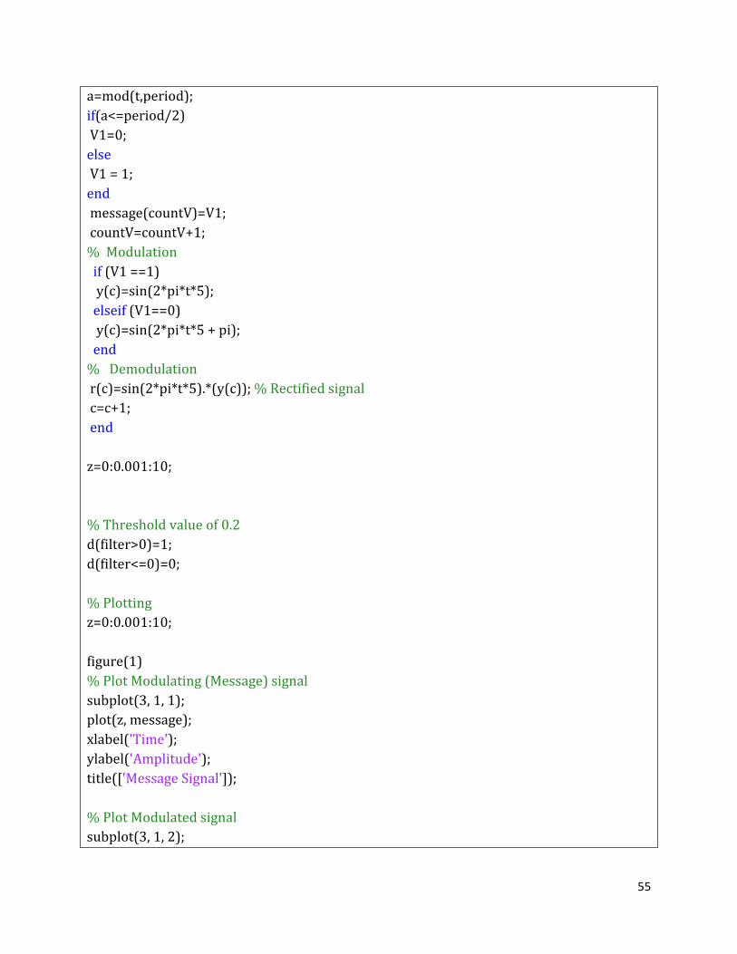
55

a=mod(t,period); if(a<=period/2) V1=0; else V1 = 1; end message(countV)=V1; countV=countV+1; % Modulation if (V1 ==1) y(c)=sin(2*pi*t*5); elseif (V1==0) y(c)=sin(2*pi*t*5 + pi); end % Demodulation r(c)=sin(2*pi*t*5).*(y(c)); % Rectified signal c=c+1; end z=0:0.001:10; % Threshold value of 0.2 d(filter>0)=1; d(filter<=0)=0; % Plotting z=0:0.001:10; figure(1) % Plot Modulating (Message) signal subplot(3, 1, 1); plot(z, message); xlabel('Time'); ylabel('Amplitude'); title(['Message Signal']); % Plot Modulated signal subplot(3, 1, 2);

56

plot(z,y); xlabel('Time'); ylabel('Amplitude'); title(['Modulated (BPSK) Signal']); grid on; % Plot Rectified signal subplot(3, 1, 3); plot(z,r); xlabel('Time'); ylabel('Amplitude'); title(['Rectified Signal']); grid on; figure(2); % Plot Filtered signal subplot(3, 1, 1); plot(x, filter); xlabel('Time'); ylabel('Amplitude'); title(['Filtered Signal']); grid on; subplot(3, 1, 2); plot(x, d); xlabel('Time'); ylabel('Amplitude'); title(['Demodulated Signal']); grid on

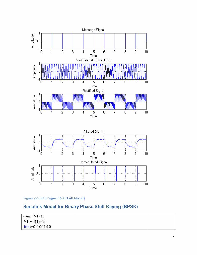
Figure 22: BPSK Signal (MATLAB Model)

Simulink Model for Binary Phase Shift Keying (BPSK)

count_V1=1; V1_val(1)=1; for t=0:0.001:10

: BPSK Signal (MATLAB Model)

Simulink Model for Binary Phase Shift Keying (BPSK)

57

58

% period=2; a=mod(t,period); if (a<=period/2) V1=0; else V1 = 1; end V1_val(count_V1)=V1; count_V1=count_V1+1; end % Input data from MATLAB to simulink Modulating signal x=[0:0.001:10]'; input_simu=[x, V1_val']; % Input to Simulink

Figure 23: Basic Building Block Diagram for BPSK System

0

Threshold

TX Carrier 2

TX Carrier 1

System Output

>=

Switch

Subtract

RX Carrier

Mixer

1

s

Integrator

input_simu

Input Signal

from Matlab

(Message)

>=

Decision

Maker

-K-

1/RC

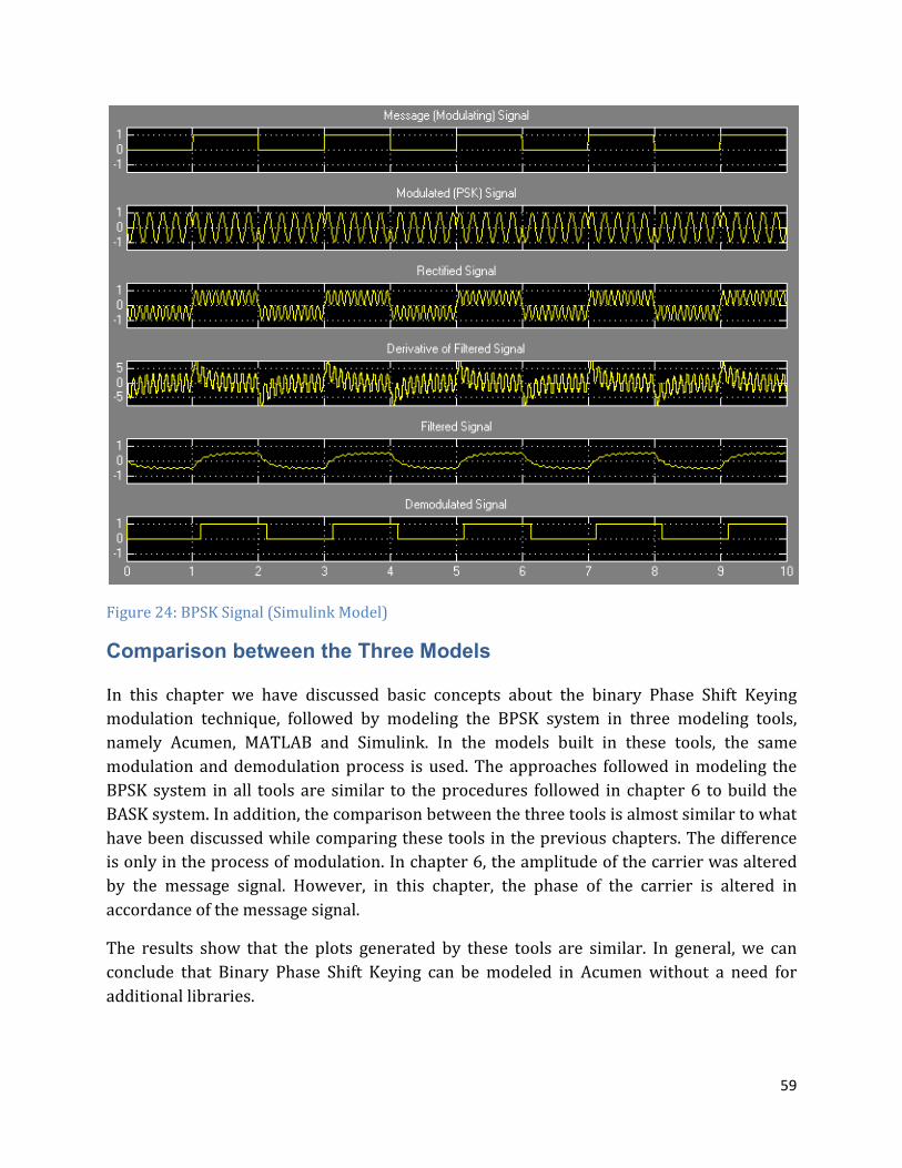
59

Figure 24: BPSK Signal (Simulink Model)

Comparison between the Three Models

In this chapter we have discussed basic concepts about the binary Phase Shift Keying modulation technique, followed by modeling the BPSK system in three modeling tools, namely Acumen, MATLAB and Simulink. In the models built in these tools, the same modulation and demodulation process is used. The approaches followed in modeling the BPSK system in all tools are similar to the procedures followed in chapter 6 to build the BASK system. In addition, the comparison between the three tools is almost similar to what have been discussed while comparing these tools in the previous chapters. The difference is only in the process of modulation. In chapter 6, the amplitude of the carrier was altered by the message signal. However, in this chapter, the phase of the carrier is altered in accordance of the message signal.

The results show that the plots generated by these tools are similar. In general, we can conclude that Binary Phase Shift Keying can be modeled in Acumen without a need for additional libraries.

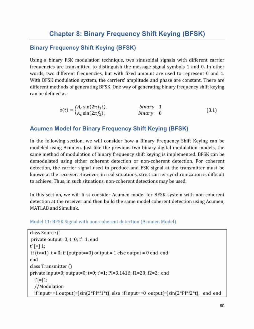
60

Chapter 8: Binary Frequency Shift Keying (BFSK)

Binary Frequency Shift Keying (BFSK)

Using a binary FSK modulation technique, two sinusoidal signals with different carrier frequencies are transmitted to distinguish the message signal symbols 1 and 0. In other words, two different frequencies, but with fixed amount are used to represent 0 and 1. With BFSK modulation system, the carriers’ amplitude and phase are constant. There are different methods of generating BFSK. One way of generating binary frequency shift keying can be defined as:

���� = $/� sin�2��4�� ,01��231/� sin�2��5� ,01��230. (8.1)

Acumen Model for Binary Frequency Shift Keying (BFSK)

In the following section, we will consider how a Binary Frequency Shift Keying can be modeled using Acumen. Just like the previous two binary digital modulation models, the same method of modulation of binary frequency shift keying is implemented. BFSK can be demodulated using either coherent detection or non-coherent detection. For coherent detection, the carrier signal used to produce and FSK signal at the transmitter must be known at the receiver. However, in real situations, strict carrier synchronization is difficult to achieve. Thus, in such situations, non-coherent detections may be used. In this section, we will first consider Acumen model for BFSK system with non-coherent detection at the receiver and then build the same model coherent detection using Acumen, MATLAB and Simulink. Model 11: BFSK Signal with non-coherent detection (Acumen Model)

class Source () private output=0; t=0; t'=1; end t' [=] 1; if (t>=1) t = 0; if (output==0) output = 1 else output = 0 end end end class Transmitter () private input=0; output=0; t=0; t'=1; PI=3.1416; f1=20; f2=2; end t'[=]1; //Modulation if input==1 output[=]sin(2*PI*f1*t); else if input==0 output[=]sin(2*PI*f2*t); end end

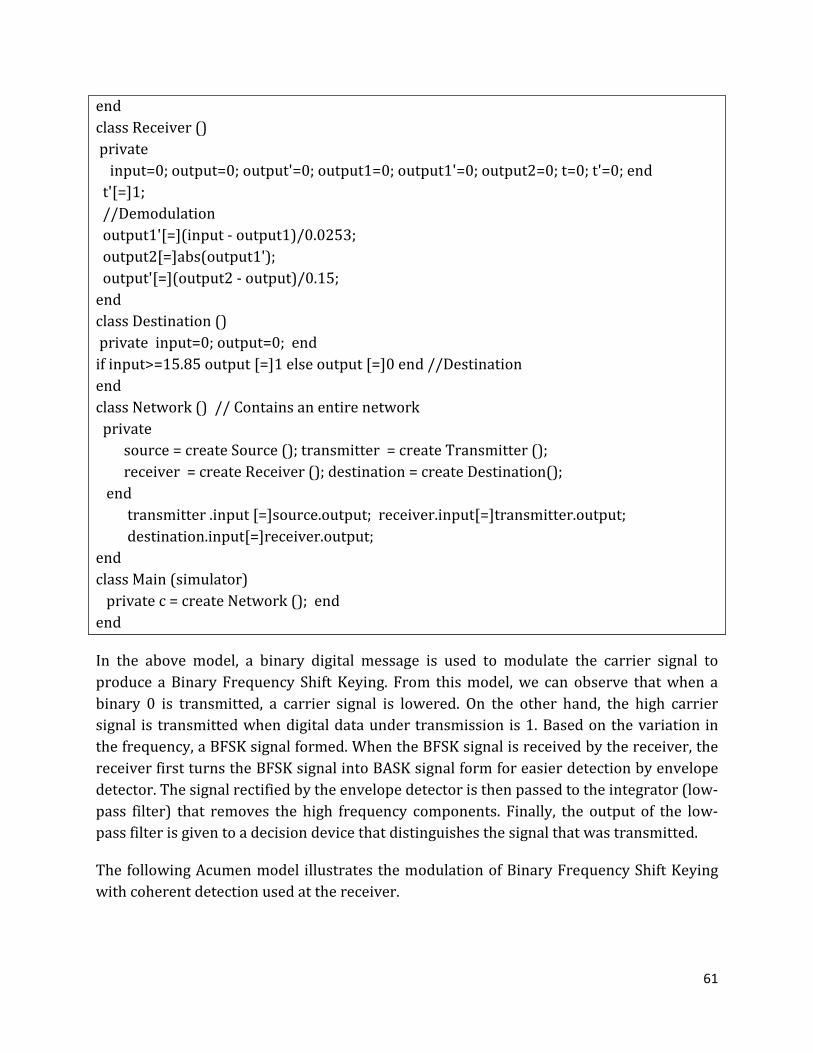
61

end class Receiver () private input=0; output=0; output'=0; output1=0; output1'=0; output2=0; t=0; t'=0; end t'[=]1; //Demodulation output1'[=](input - output1)/0.0253; output2[=]abs(output1'); output'[=](output2 - output)/0.15; end class Destination () private input=0; output=0; end if input>=15.85 output [=]1 else output [=]0 end //Destination end class Network () // Contains an entire network private source = create Source (); transmitter = create Transmitter (); receiver = create Receiver (); destination = create Destination(); end transmitter .input [=]source.output; receiver.input[=]transmitter.output; destination.input[=]receiver.output; end class Main (simulator) private c = create Network (); end end

In the above model, a binary digital message is used to modulate the carrier signal to produce a Binary Frequency Shift Keying. From this model, we can observe that when a binary 0 is transmitted, a carrier signal is lowered. On the other hand, the high carrier signal is transmitted when digital data under transmission is 1. Based on the variation in the frequency, a BFSK signal formed. When the BFSK signal is received by the receiver, the receiver first turns the BFSK signal into BASK signal form for easier detection by envelope detector. The signal rectified by the envelope detector is then passed to the integrator (low-pass filter) that removes the high frequency components. Finally, the output of the low-pass filter is given to a decision device that distinguishes the signal that was transmitted.

The following Acumen model illustrates the modulation of Binary Frequency Shift Keying with coherent detection used at the receiver.

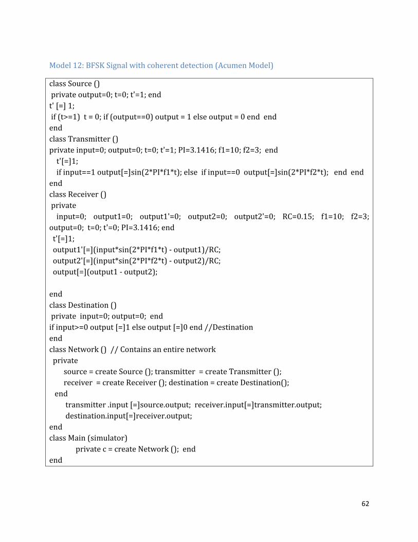
62

Model 12: BFSK Signal with coherent detection (Acumen Model)

class Source () private output=0; t=0; t'=1; end t' [=] 1; if (t>=1) t = 0; if (output==0) output = 1 else output = 0 end end end class Transmitter () private input=0; output=0; t=0; t'=1; PI=3.1416; f1=10; f2=3; end t'[=]1; if input==1 output[=]sin(2*PI*f1*t); else if input==0 output[=]sin(2*PI*f2*t); end end end class Receiver () private input=0; output1=0; output1'=0; output2=0; output2'=0; RC=0.15; f1=10; f2=3; output=0; t=0; t'=0; PI=3.1416; end t'[=]1; output1'[=](input*sin(2*PI*f1*t) - output1)/RC; output2'[=](input*sin(2*PI*f2*t) - output2)/RC; output[=](output1 - output2); end class Destination () private input=0; output=0; end if input>=0 output [=]1 else output [=]0 end //Destination end class Network () // Contains an entire network private source = create Source (); transmitter = create Transmitter (); receiver = create Receiver (); destination = create Destination(); end transmitter .input [=]source.output; receiver.input[=]transmitter.output; destination.input[=]receiver.output; end class Main (simulator) private c = create Network (); end end

63

The above model is identical to Model 11 discussed above. The only difference is the demodulation process used with this model is coherent detection. In this model, instead of turning the received BFSK signal into ASK form at the receiver, the BFSK signal is with two carriers with frequencies f1 and f2 as shown in the model and then passed to the low-pass filter. Finally, the resulting difference is given to a decision device that distinguishes the signal that was transmitted. Figure 25 shows a coherent detector for a Binary Frequency Shift Keying system.

Figure 25: Coherent Detector for a BFSK Signal

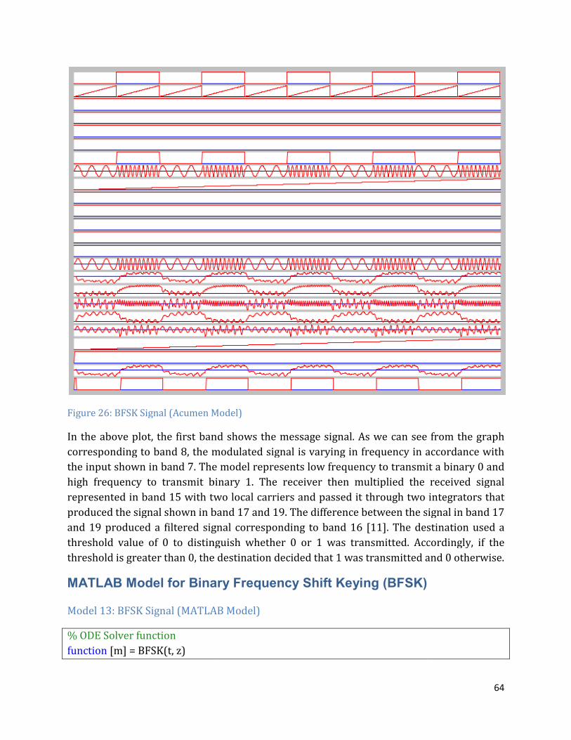
Figure 26: BFSK Signal (Acumen Model)

In the above plot, the first band shows the message signal. As we can see from the graph corresponding to band 8, the modulated signal is varying in frequency in accordance with the input shown in band 7. The model represents low frequency to transmit a binary 0 and high frequency to transmit binary 1. The receiver then multiplied the received signal represented in band 15 with two local carriers and passed it through two integrators that produced the signal shown in band 17 and 19. The difference between the signal in band and 19 produced a filtered sigthreshold value of 0 to distinguish whether 0 or 1 was transmitted. Accordingly, if the threshold is greater than 0, the destination decided that 1 was transmitted and 0 otherwise

MATLAB Model for Binary Frequency Shift Keying (BFSK)

Model 13: BFSK Signal (MATLAB

% ODE Solver function function [m] = BFSK(t, z)

: BFSK Signal (Acumen Model)

the first band shows the message signal. As we can see from the graph corresponding to band 8, the modulated signal is varying in frequency in accordance with the input shown in band 7. The model represents low frequency to transmit a binary 0 and

equency to transmit binary 1. The receiver then multiplied the received signal represented in band 15 with two local carriers and passed it through two integrators that produced the signal shown in band 17 and 19. The difference between the signal in band and 19 produced a filtered signal corresponding to band 16 [11]. The destination used a threshold value of 0 to distinguish whether 0 or 1 was transmitted. Accordingly, if the

0, the destination decided that 1 was transmitted and 0 otherwise

Model for Binary Frequency Shift Keying (BFSK)

MATLAB Model)

64

the first band shows the message signal. As we can see from the graph corresponding to band 8, the modulated signal is varying in frequency in accordance with the input shown in band 7. The model represents low frequency to transmit a binary 0 and

equency to transmit binary 1. The receiver then multiplied the received signal represented in band 15 with two local carriers and passed it through two integrators that produced the signal shown in band 17 and 19. The difference between the signal in band 17

. The destination used a threshold value of 0 to distinguish whether 0 or 1 was transmitted. Accordingly, if the

0, the destination decided that 1 was transmitted and 0 otherwise.

65

c=1; i=length(t); for j=1:1:i % Square wave period=2; a=mod(t(i),period); if (a<=period/2) V1=0; else V1 = 1; end if (V1 ==1) y(c)=sin(2*pi*t(i)*10); elseif (V1==0) y(c)=sin(2*pi*t(i)*3); end r1(c)=y(c)*sin(2*pi*t(i)*10); r2(c)=y(c)*sin(2*pi*t(i)*3); r(c) = r1(c) - r2(c); m(c) = (r(c) - z)/0.15; c=c+1; end % BFSK plotter close all; [x, filter] = ode45('BFSK', [0, 10], 0); c=1;f1=10; f2=3; countV=1; message(1)=1; for t=0:0.001:10 % square wave generator period=2; a=mod(t,period); if(a<=period/2) V1=0; else V1 = 1; end

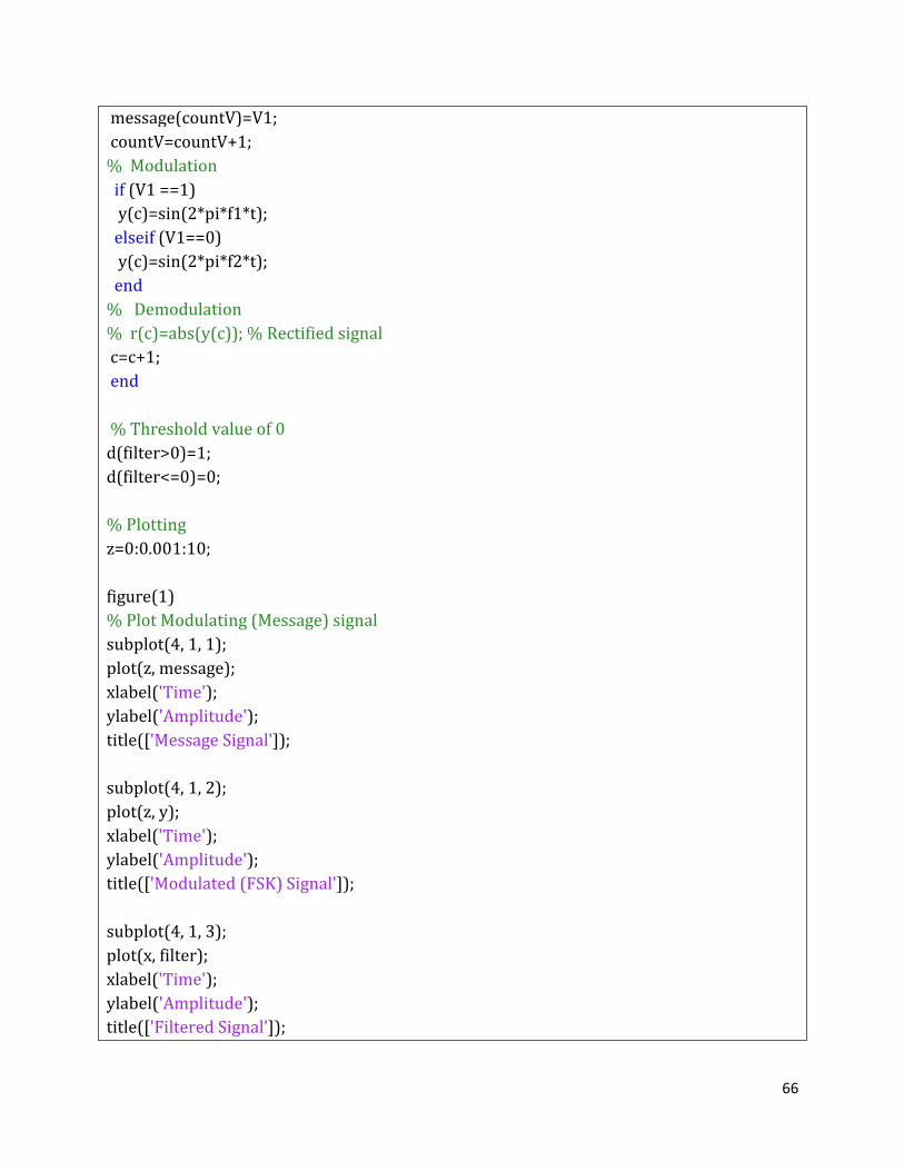
66

message(countV)=V1; countV=countV+1; % Modulation if (V1 ==1) y(c)=sin(2*pi*f1*t); elseif (V1==0) y(c)=sin(2*pi*f2*t); end % Demodulation % r(c)=abs(y(c)); % Rectified signal c=c+1; end % Threshold value of 0 d(filter>0)=1; d(filter<=0)=0; % Plotting z=0:0.001:10; figure(1) % Plot Modulating (Message) signal subplot(4, 1, 1); plot(z, message); xlabel('Time'); ylabel('Amplitude'); title(['Message Signal']); subplot(4, 1, 2); plot(z, y); xlabel('Time'); ylabel('Amplitude'); title(['Modulated (FSK) Signal']); subplot(4, 1, 3); plot(x, filter); xlabel('Time'); ylabel('Amplitude'); title(['Filtered Signal']);

67

grid on; subplot(4, 1, 4); plot(x, d); xlabel('Time'); ylabel('Amplitude'); title(['Demodulated Signal']); grid on;

The above model is built using similar methods followed to build a binary ASK, as discussed in chapter 5. The difference is that in this model, instead of varying amplitude the frequency of the modulated signal is varying in accordance with the message signal. The output of the above model is illustrated in Figure 27 below.

Figure 27: BFSK Signal (MATLAB Model)

0 1 2 3 4 5 6 7 8 9 100

0.5

1

Time

Amplitude

Message Signal

0 1 2 3 4 5 6 7 8 9 10-1

0

1

Time

Amplitude

Modulated (FSK) Signal

0 1 2 3 4 5 6 7 8 9 10-1

0

1

Time

Amplitude

Filtered Signal

0 1 2 3 4 5 6 7 8 9 100

0.5

1

Time

Amplitude

Demodulated Signal

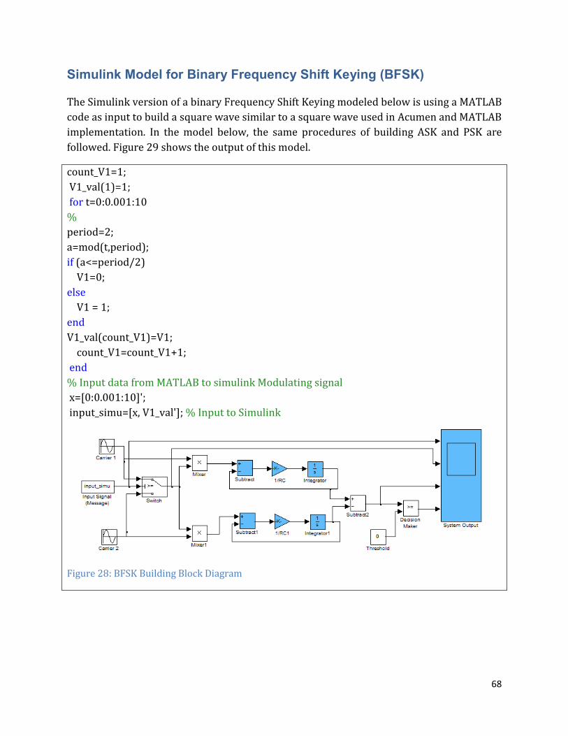
68

Simulink Model for Binary Frequency Shift Keying (BFSK)

The Simulink version of a binary Frequency Shift Keying modeled below is using a MATLAB code as input to build a square wave similar to a square wave used in Acumen and MATLAB implementation. In the model below, the same procedures of building ASK and PSK are followed. Figure 29 shows the output of this model.

count_V1=1; V1_val(1)=1; for t=0:0.001:10 % period=2; a=mod(t,period); if (a<=period/2) V1=0; else V1 = 1; end V1_val(count_V1)=V1; count_V1=count_V1+1; end % Input data from MATLAB to simulink Modulating signal x=[0:0.001:10]'; input_simu=[x, V1_val']; % Input to Simulink

Figure 28: BFSK Building Block Diagram

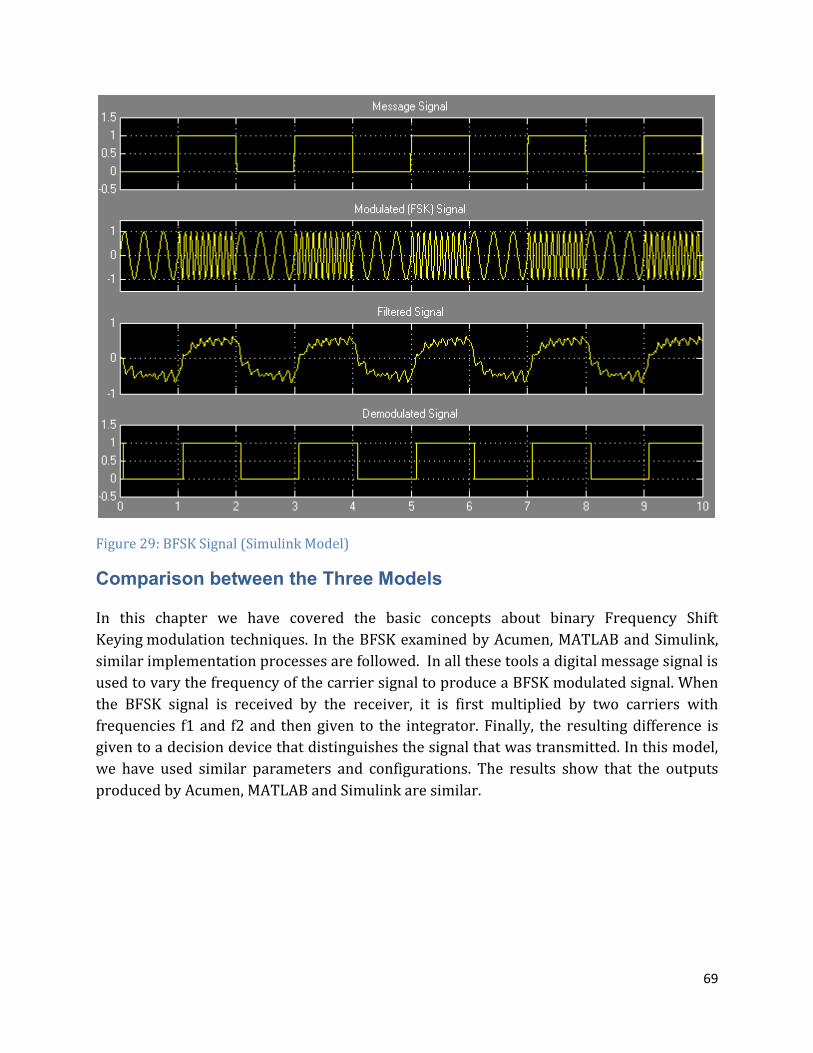
69

Figure 29: BFSK Signal (Simulink Model)

Comparison between the Three Models

In this chapter we have covered the basic concepts about binary Frequency Shift Keying modulation techniques. In the BFSK examined by Acumen, MATLAB and Simulink, similar implementation processes are followed. In all these tools a digital message signal is used to vary the frequency of the carrier signal to produce a BFSK modulated signal. When the BFSK signal is received by the receiver, it is first multiplied by two carriers with frequencies f1 and f2 and then given to the integrator. Finally, the resulting difference is given to a decision device that distinguishes the signal that was transmitted. In this model, we have used similar parameters and configurations. The results show that the outputs produced by Acumen, MATLAB and Simulink are similar.

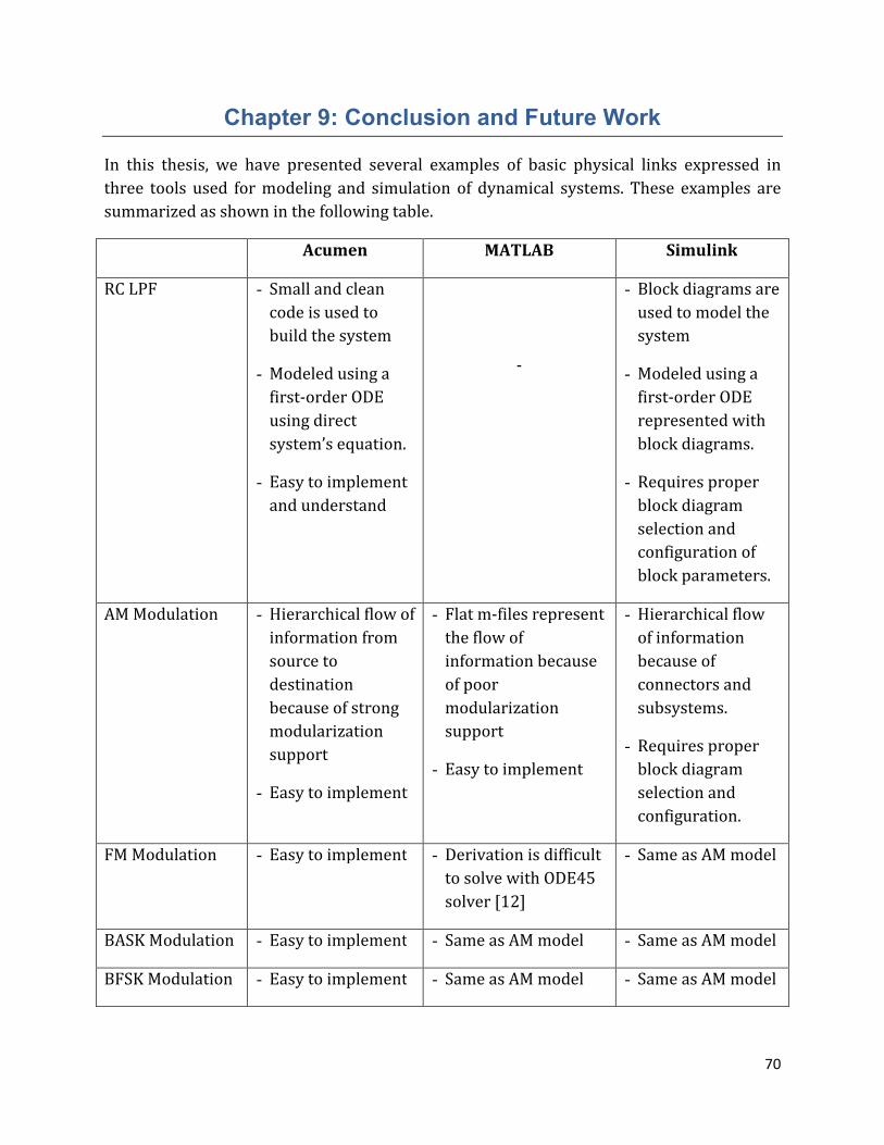
70

Chapter 9: Conclusion and Future Work

In this thesis, we have presented several examples of basic physical links expressed in three tools used for modeling and simulation of dynamical systems. These examples are summarized as shown in the following table.

Acumen MATLAB Simulink

RC LPF - Small and clean code is used to build the system

- Modeled using a first-order ODE using direct system’s equation.

- Easy to implement and understand

-

- Block diagrams are used to model the system

- Modeled using a first-order ODE represented with block diagrams.

- Requires proper block diagram selection and configuration of block parameters.

AM Modulation - Hierarchical flow of information from source to destination because of strong modularization support

- Easy to implement

- Flat m-files represent the flow of information because of poor modularization support

- Easy to implement

- Hierarchical flow of information because of connectors and subsystems.

- Requires proper block diagram selection and configuration.

FM Modulation - Easy to implement - Derivation is difficult to solve with ODE45 solver [12]

- Same as AM model

BASK Modulation - Easy to implement - Same as AM model - Same as AM model

BFSK Modulation - Easy to implement - Same as AM model - Same as AM model

71

BPSK Modulation - Easy to implement - Same as AM model - Same as AM model

In the RC low-pass filter design, two versions of Acumen model representing the same system have been presented. From those two methods, the more modular approach makes Acumen codes easy to read, to write and understand. In this approach, individual objects can be treated separately. This means that a big system is broken down into different classes so that individual components can be independently treated. Classes can be allowed to use one or more objects of other classes. This feature in Acumen enables the reusability of objects to be simple and saves resources to be allocated. Therefore, instead of defining the same object that is used with many classes in the model, a signal can be created and used by others. The benefit with this is that when the object is required to be modified, there is no need to change it everywhere other than the place where it is defined first. This is one of the advantages of Acumen in the modeling process.

As in Acumen modular approach, Simulink models can also be organized hierarchically using subsystems. Simulink subsystems are the method of adding hierarchy to a model by grouping together different blocks and encapsulating them into a single block. Once they are created, subsystems can be easily customized and manipulated as built-in blocks. Both customizable subsystems and built-in block can be reused. This can be achieved by copy and paste operations. Once we configure the required parameters for the Simulink built-in blocks and subsystems, we can copy and paste the block anywhere in the model and make use of them. The blocks retain the initial configurations when we paste them in wherever we need. However, as opposed to Acumen, when the user needs to make configuration changes to the duplicated block, the changes must be made everywhere. As we have discussed earlier, this kind of change is made only once in Acumen.

The AM system is modeled in Acumen and two other popular tools, MATLAB and Simulink. The system is examined for sinusoidal and square wave input signals in all tools. All tools have generated similar outputs for both input signal types. The differential equation used to model the low-pass filter is directly used in the Acumen model. However, this is not as simple as in Acumen for the MATLAB model to design a low-pass filter. In MATLAB, two MATLAB scripts are used to perform the integration. One script (ODE file) is a function handle that contains the ordinary differential equation to be solved. The other file (ODE solver) is used to compute the results by calling the ODE function. To plot the results, we should write a separate code. In the function handle, we need to define the signal to be passed to the differential equation. In the later script that is used to compute the results, a built-in function known as ode45 is called with this file. This adds extra tasks and complexity to solving differential equations in MATLAB.

72

In the comparison made between Acumen and the graphical Simulink model, the outputs of the system are similar.

In the digital modulation scheme, three basic digital modulation techniques called Amplitude Shift Keying, Phase Shift Keying and Frequency Shift Keying are presented. As with the previously discussed analog modulation, each of these digital modulation methods is simulated in Acumen, MATLAB and Simulink. In building these systems, the same procedures are followed. Similarly, the input signals, modulation and demodulation processes and low-pass filter designs are identical. As a result, the outputs found in each of the tools for respective modulation methods are similar.

In general, we find that, for the most part of the study, Acumen allows us to naturally express a wide range of modulation techniques, including AM, FM, ASK, PSK, and FSK. Even though it is under development, Acumen is still comparable with the popular tools like MATLAB and Simulink when modeling simple RC low-pass filter and basic modulation techniques.

When we come to general features related to these tools, we know that MATLAB and Simulink have got rich libraries and built-in functions that can be used to ease the whole modeling process. For example, when we consider Simulink, if we know how to configure different parameters for each block in the system, it needs less energy and time to build the whole system as compared to Acumen and MATLAB. However, the internal settings are not visible for readers by default. In Simulink, it is very easy to build a model by simply using a drag-and-drop operation. This graphical representation makes the model and the algorithm easy to understand. However, when it comes to practical implementation and configuration of different block parameters, special care must be taken. We need to be conversant with how each block behaves and what parameters need to be configured. Otherwise, the model may achieve undesired output.

MATLAB uses a similar textual code to Acumen. However, as MATLAB has rich built-in libraries and functions, modeling and simulation of different systems can be made simple with the help of these built-in tools. In addition, MATLAB can be used to model systems in time and frequency domains. The current version (Version 10) of Acumen does not have enough built-in libraries. Currently, Acumen supports only time domain systems. However, even though it has few libraries at this stage, the systems that can be modeled in Acumen are built with a simple algorithm like natural language. Few lines of codes can represent a big system model. For example, for a system in which its ordinary differential equation is known, the very simple and direct use of mathematical formula in Acumen code can be easily implemented. If more built-in libraries are added, Acumen could be more simple and easy to model dynamical systems.

73

The comparison made with respect to plots generated by these three tools is another feature in which these tools plot the signals. In Acumen when we run the model, the plots are automatically generated for each variable used in the model. This means that whenever we declare a variable and run the model, its plot is automatically generated by default. This has got advantages and disadvantages. The main advantage is the ability to see the value of the intended variable at any time. This is done by simply dragging the mouse cursor on the intended graph. The automatic plot generation avoids writing additional code to plot the variable. In addition, this allows us to see the effect of changing one variable on the other variables side by side. There some disadvantages with automatic plot generation. One is a lack of flexibility. For example, in some cases a user may be interested to see the plots of selected variables instead of all. However, this feature is not supported in the current version of Acumen. Lack of labelling is another disadvantage that can be observed with Acumen plots. In fact, Acumen labels each variable by default. However, this is not visible for the readers unless the graphs are labelled manually. Only developers or Acumen users can identify the plots of each variable by dragging the mouse around the plot window. The other disadvantage with plots in Acumen is that in Acumen all bands are normalized. This means that the height for each band is equal. For example, when too many variables are used in the model, the bands are highly diminished and therefore it is difficult for readers to visualize the approximated height of the signal and the signal look as a whole. The signals with height of 1 and 100 have similar look for readers. This reduces the quality of the plots.

In Simulink, in order to plot a graph for the desired variable, we need to connect each variable to the Scope block. Simulink can also make use of the MATLAB environment to produce a more readable and flexible graph. The disadvantage with this feature is that it needs extra codes to be written in MATLAB. As opposed to Acumen plots which are automatically generated, the MATLAB plots are not automatic. We need to setup a code to plot the variable of our interest with respect to time. The main advantage with MATLAB plot is its flexibility. We can customize the plots in different forms with different colors, and many plot properties. MATLAB and Simulink plots can be easily labelled.

When we compare these tools with respect to documentation, in Acumen and MATLAB we can comment each line of code to let others easily understand the code. The difference in commenting lines is that with MATLAB, comments are identified as having a different font color (green by default). This makes MATLAB comments easily understood and differentiated from executable lines. In addition, MATLAB and Simulink have rich user documentations and help integrated to the tools. Currently, Acumen does not have any user documentation and help. Debugging is one of the most important features included in MATLAB. We can debug MATLAB codes line by line. In addition, it suggests how to correct the error when it happens. However, the current version of Acumen lacks this important

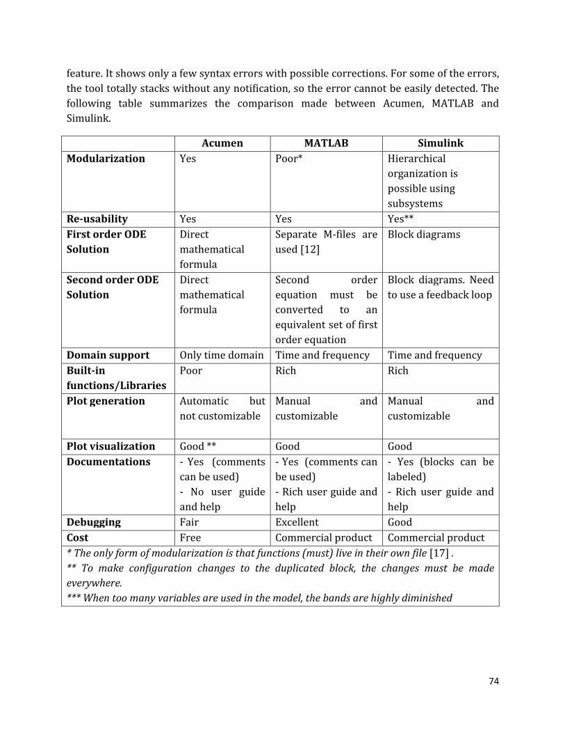
74

feature. It shows only a few syntax errors with possible corrections. For some of the errors, the tool totally stacks without any notification, so the error cannot be easily detected. The following table summarizes the comparison made between Acumen, MATLAB and Simulink.

Acumen MATLAB Simulink

Modularization Yes Poor* Hierarchical organization is possible using subsystems

Re-usability Yes Yes Yes**

First order ODE

Solution

Direct mathematical formula

Separate M-files are used [12]

Block diagrams

Second order ODE

Solution

Direct mathematical formula

Second order equation must be converted to an equivalent set of first order equation

Block diagrams. Need to use a feedback loop

Domain support Only time domain Time and frequency Time and frequency

Built-in

functions/Libraries

Poor Rich Rich

Plot generation Automatic but not customizable

Manual and customizable

Manual and customizable

Plot visualization Good ** Good Good

Documentations - Yes (comments can be used) - No user guide and help

- Yes (comments can be used) - Rich user guide and help

- Yes (blocks can be labeled) - Rich user guide and help

Debugging Fair Excellent Good

Cost Free Commercial product Commercial product

* The only form of modularization is that functions (must) live in their own file [17] .

** To make configuration changes to the duplicated block, the changes must be made

everywhere.

*** When too many variables are used in the model, the bands are highly diminished

75

Future Works

This thesis work can be further extended in different forms. One way of extension could be to consider the system by adding external noise to the signal during the transmission. Advanced modulation techniques can also be modeled and investigated. Adding basic signal types as a built-in library into Acumen is highly recommended to simplify the process of modeling different dynamical systems. In addition, a virtual experiments on higher level networking protocols need to be conducted [18].

76

References

[1] Acumen Website. [Online]. http://www.acumen-language.org/p/development.html

[2] VisSim Website. [Online]. http://www.vissim.com/products/vissim.html

[3] Claude E. Shannon, The Mathematical Theory of Communication.: University of Illinois Press, 1949.

[4] Paul Brauner, Corky Cartwright, Verónica Gaspes, Aaron Ames Waild Taha. Core Acumen. [Online].

http://www.acumen-language.org/p/tutorials.html

[5] Paul Brauner, Robert Cartwright, Verónica Gaspes, Aaron Ames, Alexandre Chapoutot Walid Taha,

"A core language for executable models of cyber physical systems: work in progress report," ACM,

vol. 8, no. 2, p. 5, 2011.

[6] The Math Works Inc., Simulink, Dynamic System Simulation for MATLAB, 3rd ed., 1999.

[7] Abhishek Yadav, Analog Communication System.: Laxmi Publications, 2008.

[8] William Palm William J Palm III, Introduction to Matlab 7 for Engineers, 2nd ed.: McGraw-Hill

Science/Engineering/Math, 2003.

[9] Jean-Francois Pradat-Peyre, Véronique Viguié Donzeau-Gouge Elie Najm, "Formal Techniques for

Networked and Distributed Systems," in FORTE 2006: 26th IFIP WG 6.1 International Conference,

Paris, France, September 26-29, 2006, 2006.

[10] Mikael Olofsson, Signal Theory, 1st ed.: Holmbergs i Malmö AB, Sweden, 2011.

[11] Mao-Ching Chiu, Jung-Shan Lin Richard Chia Tung Lee, Communications Engineering: Essentials for

Computer Scientists and Electrical Engineers, 1st ed., 2007.

[12] Duane Hanselman, Mastering MATLAB 7.: Pearson Education International, 2005.

[13] Behrouz Forouzan, Data Communications and Networking, 3rd ed.: McGraw-Hill, 2003.

[14] Wai-Kai Chen, Electrical Engineering Handbook, 1st ed.: Elsevier Academic Press, 2005.

[15] Peter M. Grant Ian A. Glover, Digital Communications, 2nd ed.: Prentice Hall, 2003.

[16] Omer Farook and C.R. Sekhar Jai P. Agrawal, "SIMULINK Laboratory Exercises In Communication

Technology," in American Society for Engineering Education Annual Conference Exposition, 2005.

[17] Grant Griffin, Iowegian International Corporation. Life Without Matlab (Powepoint Presentation).

77

[Online]. http://www.compdsp.com/presentations/Griffin/Life_Without_Matlab.pdf

[18] Consel, O’Malley, Taha, Hannourah Bruneau, "Virtual Testing for Smart Buildings," in 8th

International Conference on Intelligent Environments (IE), 2012. [Online].

http://dl.dropbox.com/u/17132045/p/publications/conference/IE12.pdf

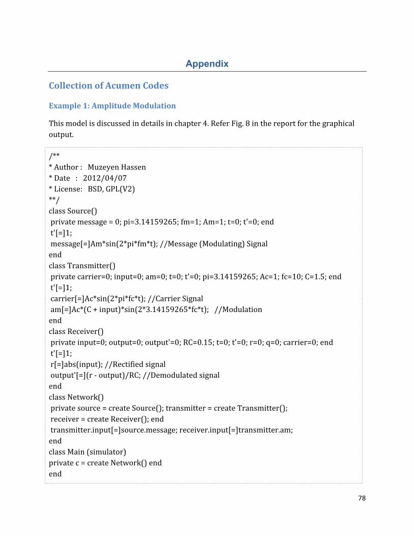
78

Appendix

Collection of Acumen Codes

Example 1: Amplitude Modulation

This model is discussed in details in chapter 4. Refer Fig. 8 in the report for the graphical output.

/** * Author : Muzeyen Hassen * Date : 2012/04/07 * License: BSD, GPL(V2) **/ class Source() private message = 0; pi=3.14159265; fm=1; Am=1; t=0; t'=0; end t'[=]1; message[=]Am*sin(2*pi*fm*t); //Message (Modulating) Signal end class Transmitter() private carrier=0; input=0; am=0; t=0; t'=0; pi=3.14159265; Ac=1; fc=10; C=1.5; end t'[=]1; carrier[=]Ac*sin(2*pi*fc*t); //Carrier Signal am[=]Ac*(C + input)*sin(2*3.14159265*fc*t); //Modulation end class Receiver() private input=0; output=0; output'=0; RC=0.15; t=0; t'=0; r=0; q=0; carrier=0; end t'[=]1; r[=]abs(input); //Rectified signal output'[=](r - output)/RC; //Demodulated signal end class Network() private source = create Source(); transmitter = create Transmitter(); receiver = create Receiver(); end transmitter.input[=]source.message; receiver.input[=]transmitter.am; end class Main (simulator) private c = create Network() end end

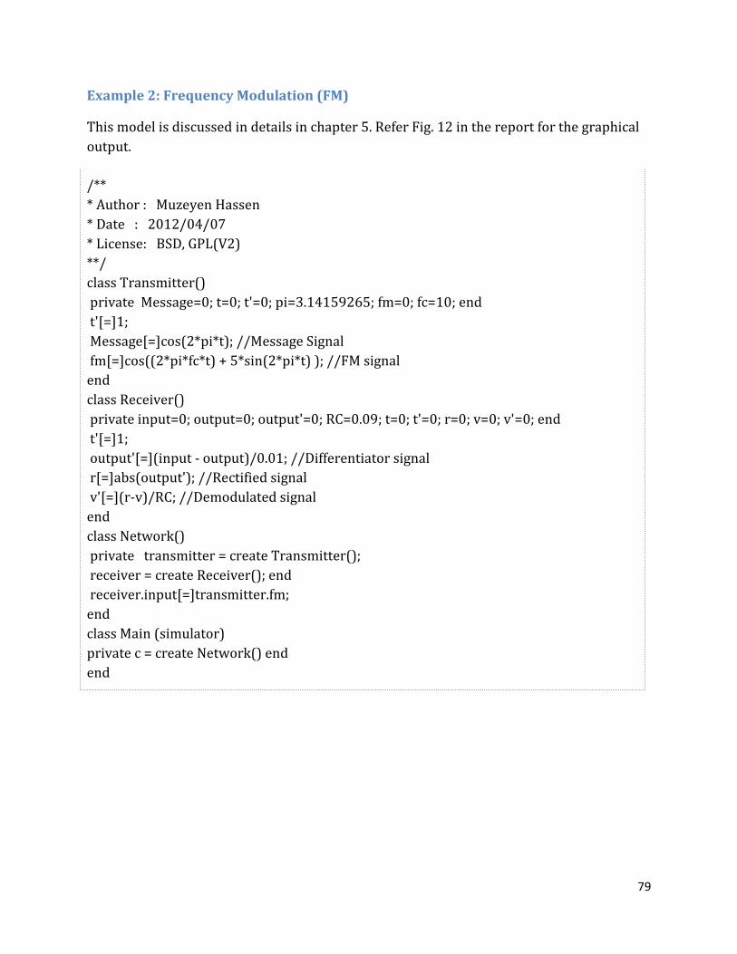
79

Example 2: Frequency Modulation (FM)

This model is discussed in details in chapter 5. Refer Fig. 12 in the report for the graphical output.

/** * Author : Muzeyen Hassen * Date : 2012/04/07 * License: BSD, GPL(V2) **/ class Transmitter() private Message=0; t=0; t'=0; pi=3.14159265; fm=0; fc=10; end t'[=]1; Message[=]cos(2*pi*t); //Message Signal fm[=]cos((2*pi*fc*t) + 5*sin(2*pi*t) ); //FM signal end class Receiver() private input=0; output=0; output'=0; RC=0.09; t=0; t'=0; r=0; v=0; v'=0; end t'[=]1; output'[=](input - output)/0.01; //Differentiator signal r[=]abs(output'); //Rectified signal v'[=](r-v)/RC; //Demodulated signal end class Network() private transmitter = create Transmitter(); receiver = create Receiver(); end receiver.input[=]transmitter.fm; end class Main (simulator) private c = create Network() end end

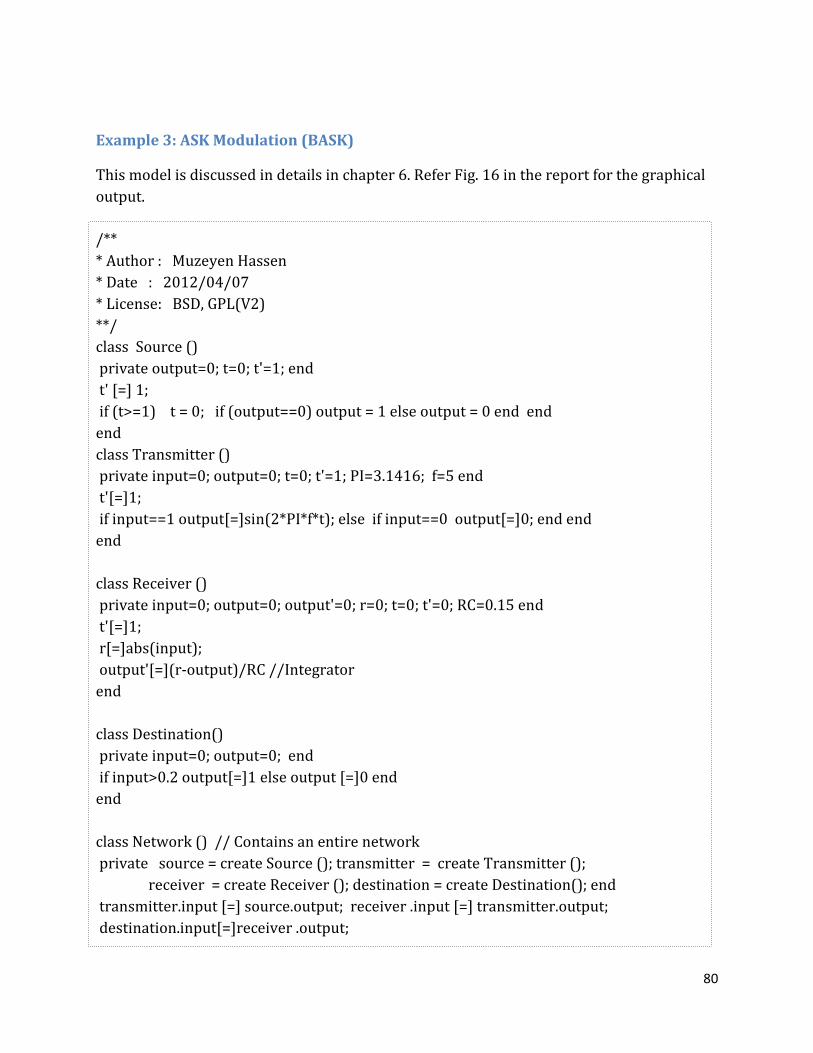
80

Example 3: ASK Modulation (BASK)

This model is discussed in details in chapter 6. Refer Fig. 16 in the report for the graphical output.

/** * Author : Muzeyen Hassen * Date : 2012/04/07 * License: BSD, GPL(V2) **/ class Source () private output=0; t=0; t'=1; end t' [=] 1; if (t>=1) t = 0; if (output==0) output = 1 else output = 0 end end end class Transmitter () private input=0; output=0; t=0; t'=1; PI=3.1416; f=5 end t'[=]1; if input==1 output[=]sin(2*PI*f*t); else if input==0 output[=]0; end end end class Receiver () private input=0; output=0; output'=0; r=0; t=0; t'=0; RC=0.15 end t'[=]1; r[=]abs(input); output'[=](r-output)/RC //Integrator end class Destination() private input=0; output=0; end if input>0.2 output[=]1 else output [=]0 end end class Network () // Contains an entire network private source = create Source (); transmitter = create Transmitter (); receiver = create Receiver (); destination = create Destination(); end transmitter.input [=] source.output; receiver .input [=] transmitter.output; destination.input[=]receiver .output;

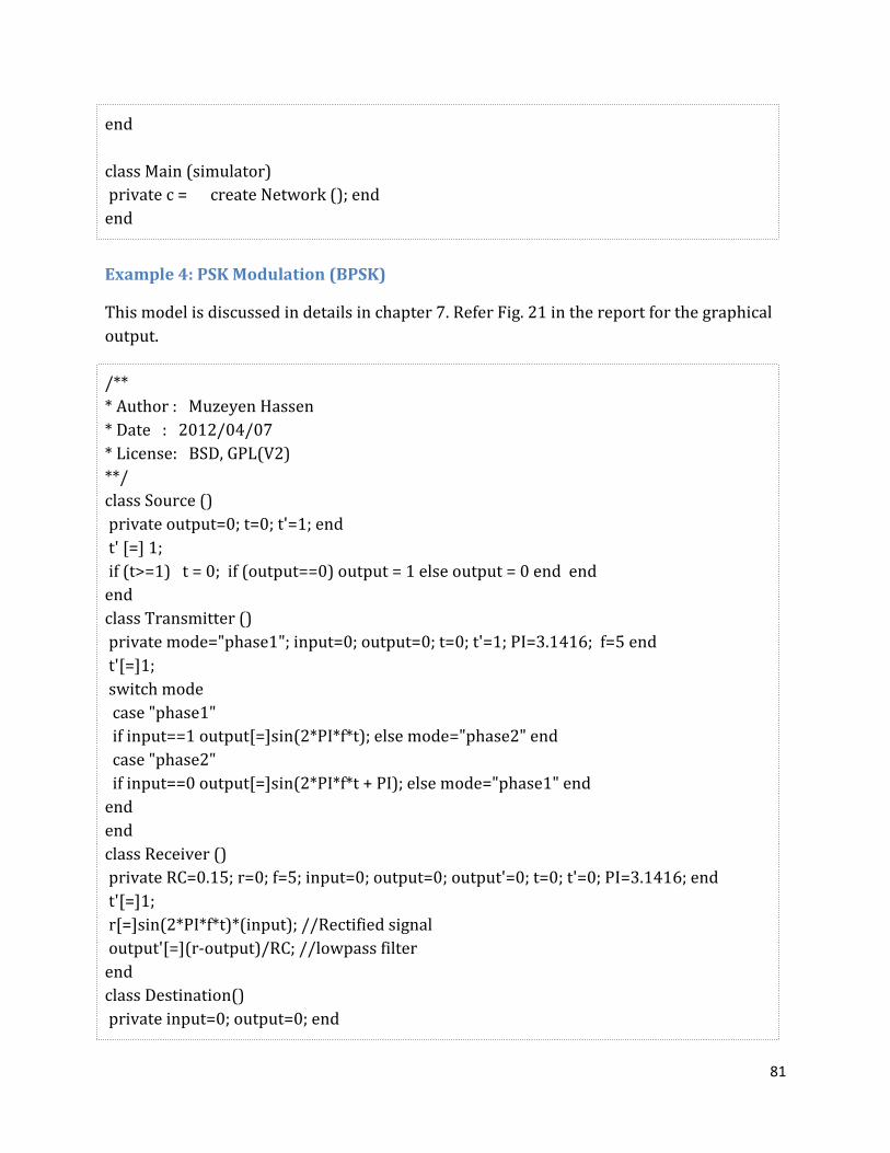
81

end class Main (simulator) private c = create Network (); end end

Example 4: PSK Modulation (BPSK)

This model is discussed in details in chapter 7. Refer Fig. 21 in the report for the graphical output.

/** * Author : Muzeyen Hassen * Date : 2012/04/07 * License: BSD, GPL(V2) **/ class Source () private output=0; t=0; t'=1; end t' [=] 1; if (t>=1) t = 0; if (output==0) output = 1 else output = 0 end end end class Transmitter () private mode="phase1"; input=0; output=0; t=0; t'=1; PI=3.1416; f=5 end t'[=]1; switch mode case "phase1" if input==1 output[=]sin(2*PI*f*t); else mode="phase2" end case "phase2" if input==0 output[=]sin(2*PI*f*t + PI); else mode="phase1" end end end class Receiver () private RC=0.15; r=0; f=5; input=0; output=0; output'=0; t=0; t'=0; PI=3.1416; end t'[=]1; r[=]sin(2*PI*f*t)*(input); //Rectified signal output'[=](r-output)/RC; //lowpass filter end class Destination() private input=0; output=0; end

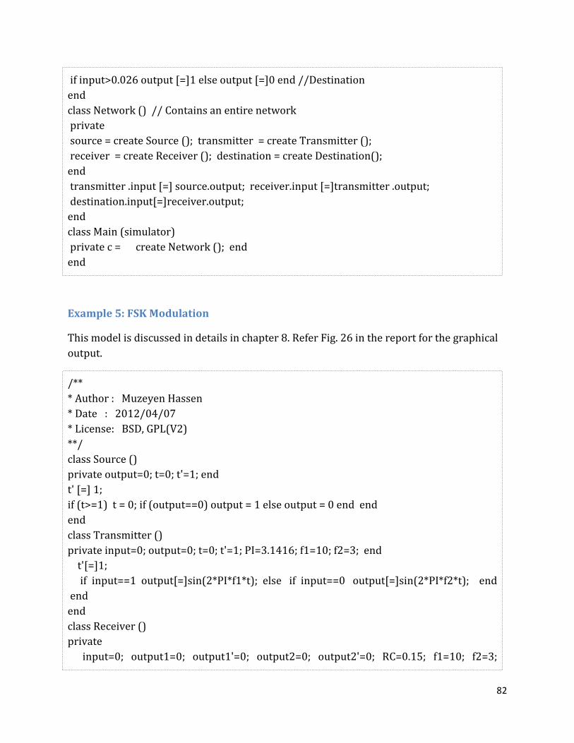
82

if input>0.026 output [=]1 else output [=]0 end //Destination end class Network () // Contains an entire network private source = create Source (); transmitter = create Transmitter (); receiver = create Receiver (); destination = create Destination(); end transmitter .input [=] source.output; receiver.input [=]transmitter .output; destination.input[=]receiver.output; end class Main (simulator) private c = create Network (); end end

Example 5: FSK Modulation

This model is discussed in details in chapter 8. Refer Fig. 26 in the report for the graphical output.

/** * Author : Muzeyen Hassen * Date : 2012/04/07 * License: BSD, GPL(V2) **/ class Source () private output=0; t=0; t'=1; end t' [=] 1; if (t>=1) t = 0; if (output==0) output = 1 else output = 0 end end end class Transmitter () private input=0; output=0; t=0; t'=1; PI=3.1416; f1=10; f2=3; end t'[=]1; if input==1 output[=]sin(2*PI*f1*t); else if input==0 output[=]sin(2*PI*f2*t); end end end class Receiver () private input=0; output1=0; output1'=0; output2=0; output2'=0; RC=0.15; f1=10; f2=3;

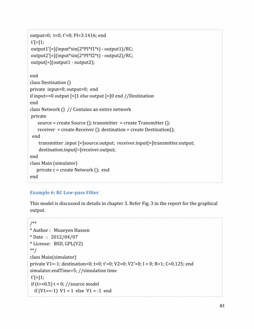
83

output=0; t=0; t'=0; PI=3.1416; end t'[=]1; output1'[=](input*sin(2*PI*f1*t) - output1)/RC; output2'[=](input*sin(2*PI*f2*t) - output2)/RC; output[=](output1 - output2); end class Destination () private input=0; output=0; end if input>=0 output [=]1 else output [=]0 end //Destination end class Network () // Contains an entire network private source = create Source (); transmitter = create Transmitter (); receiver = create Receiver (); destination = create Destination(); end transmitter .input [=]source.output; receiver.input[=]transmitter.output; destination.input[=]receiver.output; end class Main (simulator) private c = create Network (); end end

Example 6: RC Low-pass Filter

This model is discussed in details in chapter 3. Refer Fig. 3 in the report for the graphical output.

/** * Author : Muzeyen Hassen * Date : 2012/04/07 * License: BSD, GPL(V2) **/ class Main(simulator) private V1=-1; destination=0; t=0; t'=0; V2=0; V2'=0; I = 0; R=1; C=0.125; end simulator.endTime=5; //simulation time t'[=]1; if (t>=0.5) t = 0; //source model if (V1==-1) V1 = 1 else V1 = -1 end

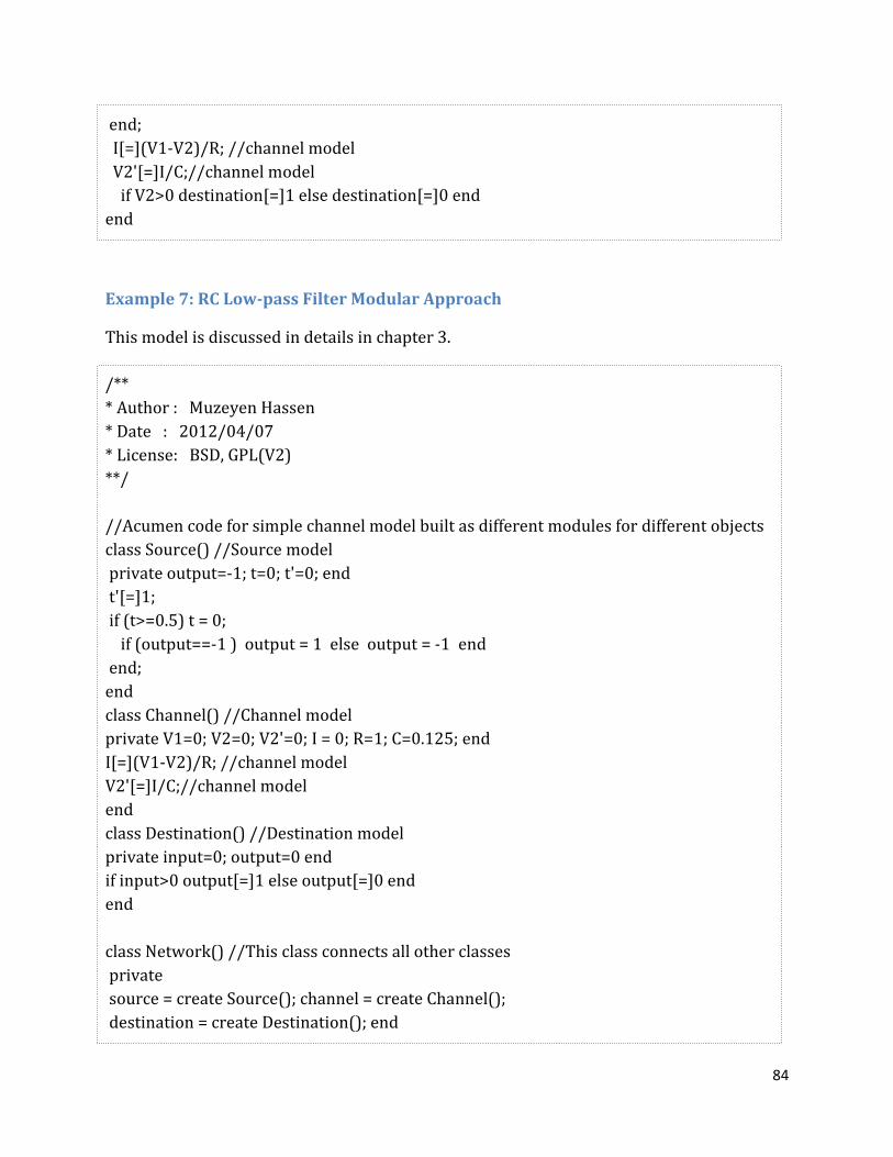
84

end; I[=](V1-V2)/R; //channel model V2'[=]I/C;//channel model if V2>0 destination[=]1 else destination[=]0 end end

Example 7: RC Low-pass Filter Modular Approach

This model is discussed in details in chapter 3.

/** * Author : Muzeyen Hassen * Date : 2012/04/07 * License: BSD, GPL(V2) **/ //Acumen code for simple channel model built as different modules for different objects class Source() //Source model private output=-1; t=0; t'=0; end t'[=]1; if (t>=0.5) t = 0; if (output==-1 ) output = 1 else output = -1 end end; end class Channel() //Channel model private V1=0; V2=0; V2'=0; I = 0; R=1; C=0.125; end I[=](V1-V2)/R; //channel model V2'[=]I/C;//channel model end class Destination() //Destination model private input=0; output=0 end if input>0 output[=]1 else output[=]0 end end class Network() //This class connects all other classes private source = create Source(); channel = create Channel(); destination = create Destination(); end

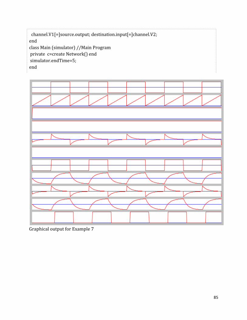
channel.V1[=]source.output; destination.input[=]channel.V2;end class Main (simulator) //Main Program private c=create Network() end simulator.endTime=5; end

Graphical output for Example 7

channel.V1[=]source.output; destination.input[=]channel.V2;

Main (simulator) //Main Program c=create Network() end

7

85