thesis by martin regehr
TRANSCRIPT
Signal Extraction and Control for anInterferometric Gravitational Wave Detector
Thesis by
Martin W. Regehr
In Partial Fulfillment of the Requirementsfor the Degreeof
Doctor of Philosophy
California Institute of TechnologyPasadena,California
1995
(SubmittedAugust 1, 1994)

To my Father
ii
Acknowledgements
I am indebted to my three advisors: to Ron Drever, who accepted me
into the LIGO team, to Fred Raab, without whose tremendous patience and
valuable suggestions my experiment might never have been completed, and whose
painstaking reading of this thesis eliminated countless errors therefrom, and to
Amnon Yariv, whose interest, enthusiasm, and kindness have been a constant
source of inspiration for me.
I am also grateful to the entire LIGO team, whose support, technical and
emotional, has been invaluable during my stay at Caltech, and especially to
Alex Abramovici, Jake Chapsky, Torrey Lyons, David Shoemaker, Lisa Sievers
and Stan Whitcomb, each of whom contributed very substantially to the work
described herein.
iii
Abstract
Large interferometersare currently under constructionfor the detectionof
gravitationalradiation. Thesewill containa numberof optical surfacesat each
of which the relativephaseof incidentbeamsmustbe kept strictly controlledin
order to achievehigh sensitivity.
Thetypeof interferometerconsideredhereconsistsof two Fabry-Perotcavities
illuminatedby a laserbeamwhich is split in half by a beamsplitter,togetherwith
a recycling mirror betweenthe laserand the beamsplitter, which reflectslight
returningfrom the beamsplitter towardthe laserbackinto the interferometer.A
schemefor sensingdeviationsfrom properinterferencehasbeenanalyzedandthe
adequacyof this methodfor incorporationin a controlsystemhasbeenevaluated.
The sensingschemeinvolves phasemodulatingthe laser light incident on the
interferometer,introducinganasymmetryin thedistancesbetweentheFabry-Perot
cavitiesandthe beamsplitter, anddemodulatingthe signalsfrom photodetectors
monitoring three optical outputs of the interferometer. Theseoptical outputs
are light returning to the laser, light extractedby a pick-off from betweenthe
recyclingmirror andthe beamsplitter, andlight leavingthe interferometerat the
beamsplitter.
The analysishas shown that the matrix of transfer functions from mirror
displacementto demodulatedsignal is ill-conditioned, that as many as threeof
iv
the transferfunctionsmay containright half planezeros,and that one of these
transferfunctionscanbe affectedby the modulationdepth. The performanceof
theclosed-loopsystem,however,neednot besignificantlyaffected,providedthat
certainconstraintsareobservedin the optical andelectronicdesign.
A table-topinterferometerhasbeenconstructed,to demonstratethefeasibility
of constructinga control systemusing this sensingschemeand to comparethe
responseof theinterferometerwith thatpredictedby calculations.Goodagreement
betweenthe experimentand the calculationhasbeenobtained.
v
Contents
. . . . . . . . . . . . . . . . . . . . . . . . . . . . . . . . . . . . . . . . . . . . ii
Acknowledgements . . . . . . . . . . . . . . . . . . . . . . . . . . . . . . . . iii
Abstract . . . . . . . . . . . . . . . . . . . . . . . . . . . . . . . . . . . . . . . iv
List of Tables . . . . . . . . . . . . . . . . . . . . . . . . . . . . . . . . . . . . ix
List of Figures . . . . . . . . . . . . . . . . . . . . . . . . . . . . . . . . . . . x
Table of Mathematical Symbols . . . . . . . . . . . . . . . . . . . . . . . xiv
Chapter 1 Introduction . . . . . . . . . . . . . . . . . . . . . . . . . 1
Chapter 2 DC Analysis . . . . . . . . . . . . . . . . . . . . . . . . 15
Photodetector, Mixer . . . . . . . . . . . . . . . . . 17
Fields in Optical Cavities . . . . . . . . . . . . . . 19
Fields in the Interferometer . . . . . . . . . . . . . 22
Derivatives of Mixer Outputs . . . . . . . . . . . . 31
Chapter 3 Interferometer Frequency Response . . . . . . . . . 40
Fabry-Perot Cavity . . . . . . . . . . . . . . . . . . 40
Response of the Complete Interferometer . . . . 53
vi
Chapter 4 Numerical Models . . . . . . . . . . . . . . . . . . . . 64
Chapter 5 Experiments with the Table-top Prototype . . . . . 72
Setup and Hardware . . . . . . . . . . . . . . . . . 73
Component Response Measurements . . . . . . 78
Response of a Fabry-Perot Cavity . . . . . . . . 81
Response of the Coupled-Cavity . . . . . . . . . 82
Response of the Complete Interferometer . . . . 86
Chapter 6 Design and Analysis of a Control System . . . . . 98
Feedback Configuration and Gain Constraint . 101
System Performance . . . . . . . . . . . . . . . 108
Numerical Example of a Control System
Design . . . . . . . . . . . . . . . . . . . . . . . . . 114
Chapter 7 Optical Design Considerations . . . . . . . . . . . 122
Common-mode Feedback Configuration . . . . 122
Asymmetry . . . . . . . . . . . . . . . . . . . . . . 123
Recycling Mirror Reflectivity . . . . . . . . . . . 125
Modulation Index . . . . . . . . . . . . . . . . . . 126
Arm Cavity and Recycling Cavity Lengths . . . 129
vii
Chapter 8 Summary and Conclusion . . . . . . . . . . . . . . 130
Robustness . . . . . . . . . . . . . . . . . . . . . . 131
Lock Acquisition . . . . . . . . . . . . . . . . . . . 134
Conclusion . . . . . . . . . . . . . . . . . . . . . . 135
Appendix A Shot Noise at the Mixer Output . . . . . . . . . . . 140
Appendix B Specification of Allowable RMS Deviations from
Perfect Resonance . . . . . . . . . . . . . . . . . . . 149
Introduction . . . . . . . . . . . . . . . . . . . . . . 149
Power in the Arm Cavities . . . . . . . . . . . . 150
Frequency Noise . . . . . . . . . . . . . . . . . . 151
Intensity Noise . . . . . . . . . . . . . . . . . . . . 152
Dark at the Antisymmetric Output . . . . . . . . 152
Summary . . . . . . . . . . . . . . . . . . . . . . . 153
Appendix C Alternative Feedback Configurations . . . . . . . 156
Appendix D Effect of Mixer Phase Error . . . . . . . . . . . . . 163
viii

List of Tables
Table 1.1 Possible optical parameters for a LIGO
interferometer. . . . . . . . . . . . . . . . . . . . . . . 13
Table 2.1 Vanishing terms in equation (2.6) for derivatives of
��� and ��� with respect to the differential degrees of
freedom. . . . . . . . . . . . . . . . . . . . . . . . . . 37
Table 2.2 Vanishing terms in equation (2.8) for derivatives of
��� and ��� with respect to the differential degrees of
freedom. . . . . . . . . . . . . . . . . . . . . . . . . . 37
Table 5.1 Results of Coupled-Cavity Experiments . . . . . . . 86
Table 5.2 Fixed Mass Interferometer Optical Properties . . . 87
Table 5.3 Sampled values of experimental (bold) and
calculated response. . . . . . . . . . . . . . . . . . . 94
Table 6.1 Loop shapes and performance predictions for
numerical servo design. . . . . . . . . . . . . . . . . 121
ix

List of Figures
Figure 1.1 Effect that a horizontally propagating gravitational
wave might have on a human being. . . . . . . . . . 2
Figure 1.2 Michelson interferometer. . . . . . . . . . . . . . . . . 2
Figure 1.3 Interferometer with Fabry-Perot arms. . . . . . . . . . 4
Figure 1.4 Interferometer with power recycling. . . . . . . . . . . 5
Figure 1.5 Interferometer, showing mirror suspensions. . . . . 6
Figure 1.6 Signal extraction scheme. . . . . . . . . . . . . . . . . 7
Figure 1.7 Feedback configuration. . . . . . . . . . . . . . . . . . 9
Figure 2.1 Example of a section of laser beam. . . . . . . . . 15
Figure 2.2 Partially transmitting mirror. . . . . . . . . . . . . . . 19
Figure 2.3 Fabry-Perot cavity. . . . . . . . . . . . . . . . . . . . . 20
Figure 2.4 Fields at in-line arm cavity. . . . . . . . . . . . . . . 22
Figure 2.5 Fields at beam splitter and pick-off. . . . . . . . . . 24
Figure 2.6 Compound mirror. . . . . . . . . . . . . . . . . . . . . 25
Figure 2.7 Equivalent optical configuration for the analysis of
sideband fields. . . . . . . . . . . . . . . . . . . . . . 28
Figure 2.8 Compound mirror for the RF sidebands. . . . . . . 30
Figure 3.1 Fabry-Perot cavity. . . . . . . . . . . . . . . . . . . . 41
x
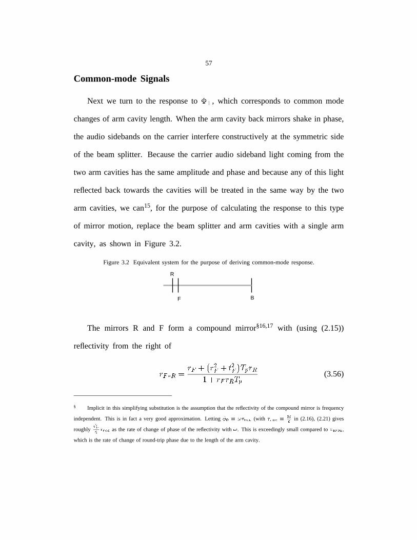
Figure 3.2 Equivalent system for the purpose of deriving
common-mode response. . . . . . . . . . . . . . . . 57
Figure 4.1 Table of numerical (upper) and approximate analytic
(lower) derivatives of interferometer outputs, for the
optical parameters given in Table 1.1. . . . . . . . 69
Figure 4.2 Frequency response curves calculated using the
approximate analytical method and (dashed) the
strictly numerical model. . . . . . . . . . . . . . . . . 70
Figure 5.1 RF Distribution. . . . . . . . . . . . . . . . . . . . . . . 75
Figure 5.2 Schematic representation of a high voltage
amplifier and the dynamic signal analyzer. . . . . . 77
Figure 5.3 Displacement transducer characterization. . . . . . 79
Figure 5.4 Measuring the modulation index. . . . . . . . . . . . 80
Figure 5.5 Measurement of the response of a Fabry-Perot
cavity. . . . . . . . . . . . . . . . . . . . . . . . . . . . 81
Figure 5.6 Coupled-cavity experiment. . . . . . . . . . . . . . . 83
Figure 5.7 Block diagram of the control system for the
coupled-cavity experiment. . . . . . . . . . . . . . . 84
Figure 5.8 Layout of complete interferometer. . . . . . . . . . . 88
Figure 5.9 Servo configuration of Table-top prototype.
Feedback amplifiers not shown. . . . . . . . . . . . 89
xi
Figure 5.10 Time record of lock interruption. . . . . . . . . . . . 91
Figure 5.11 Block diagram representing setup for closed loop
measurements. . . . . . . . . . . . . . . . . . . . . . . 92
Figure 5.12 Setup for measuring the factors���
and ��� . . . . . 93
Figure 5.13 Plots of experimental and calculated (dashed)
response. . . . . . . . . . . . . . . . . . . . . . . . . . 96
Figure 6.1 Equivalent block diagrams for the plant. . . . . . . 99
Figure 6.2 Closed-loop system. . . . . . . . . . . . . . . . . . . . 99
Figure 6.3 Closed-loop system with a diagonal controller. . 100
Figure 6.4 Closed-loop system with a “crossed” controller. . 100
Figure 6.5 Block diagram for analysis of system containing
frequency-independent plant. . . . . . . . . . . . . . 102
Figure 6.6 Block diagram used to analyze performance,
showing inputs driven by seismic disturbance. . . 108
Figure 6.7 Block diagram showing plant and one feedback
loop as a single block. . . . . . . . . . . . . . . . . . 110
Figure 6.8 Seismic spectrum. . . . . . . . . . . . . . . . . . . . 117
Figure 6.9 Block diagram for the propagation of seismic
disturbance. . . . . . . . . . . . . . . . . . . . . . . . . 118
xii
Figure 6.10 Loop gains (a)) and residual motion (b)) in
common-mode degrees of freedom. Curves
corresponding to the���
loop are dashed. . . . . 119
Figure 6.11 Contributions from loop 1 and loop 2 (dashed) to
residual deviations from resonance in loop 1 (a)
and in loop 2 (b). . . . . . . . . . . . . . . . . . . . . 120
Figure C.1 First alternative configuration: feed-back to beam
splitter. . . . . . . . . . . . . . . . . . . . . . . . . . . . 156
Figure C.2 Second alternative feedback configuration. . . . 160
Figure D.1 Block diagram used to analyze the effect of mixer
phase error. . . . . . . . . . . . . . . . . . . . . . . . . 164
xiii

Table of Mathematical Symbols
Symbol Page number���,���
, � � , � � , � , ��� � , ���� � 6��� , ��� , ��� , ��� 8���10���11� �10� �11�16�16� �
,� !#"�$
16%'&17� � , ��( 18) 19*19+
,+-,
21) $/.0�1��2 23) $43 , ) ,$53 236
, 7 25� 8,� 9
,� :<; � ,
� 8>=@? �,� 8>=0? �
,�BAC"D?E!
24)GFIH ,* &
23)GJ 25� 8K= 925
) $ � , ) ,$ � 27L 29+M3
,+ � 35
xiv
���� , ���� 36� 41� ��� 43��� � � � 42 44� ��� 44�
45 ������ 53 ������ 56�66�
,���
,� �
99 98!,! � , !#" 99$ � , $ " , �%� , & � , & " , � � , � " 101� � , � " 105' � , '(" , ) � , ) " 108�
109*, + � , + " 111
xv
1
Chapter 1 Introduction
In the year 1915, Albert Einstein publisheda theory which he called the
Generaltheory of Relativity. This theory interpretsthe force of gravity as a
distortion of spaceand time producedby objectswith mass. The theory also
predictsthat wave-likedistortionsof spaceandtime be able to propagateacross
the universe,in a fashionsimilar to the propagationof electromagneticwaves.
Thesewaveswould be producedby acceleratingmass,muchaselectromagnetic
wavesareproducedby acceleratingcharge. The direct detectionof thesewaves
would providea strongconfirmationof Einstein’stheory. Their observationwith
good signal-to-noiseratio could provide a wealth of new information about the
universe,sincemostanticipatedsourcesof gravitationalradiationaredifficult to
observeoptically.
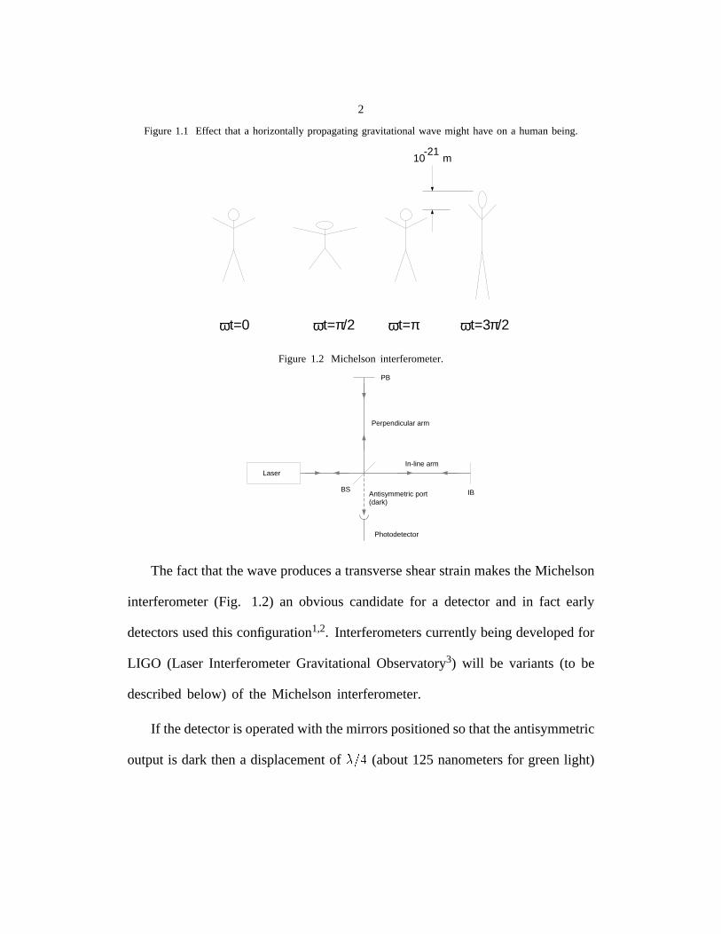
Although the Generaltheory of Relativity is conceptuallyquite subtle, the
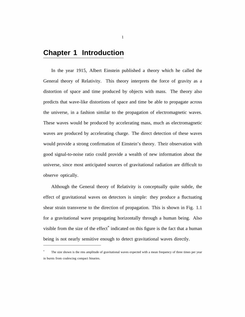
effect of gravitationalwaveson detectorsis simple: they producea fluctuating
shearstrain transverseto the directionof propagation.This is shownin Fig. 1.1
for a gravitationalwave propagatinghorizontally througha humanbeing. Also
visible from thesizeof theeffect* indicatedon this figure is thefact thata human
being is not nearlysensitiveenoughto detectgravitationalwavesdirectly.
* The sizeshownis the rms amplitudeof gravitationalwavesexpectedwith a meanfrequencyof threetimesperyear
in burstsfrom coalescingcompactbinaries.
2
Figure1.1 Effect that a horizontallypropagatinggravitationalwavemight haveon a humanbeing.
ωt=0 ωt=π/2 ωt=π ωt=3π/2
10 m-21
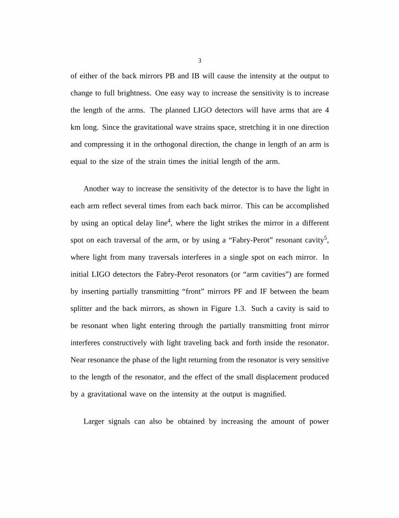
Figure 1.2 Michelson interferometer.
LaserIn-line arm
Perpendicular arm
PB
IBBS
Photodetector
Antisymmetric port(dark)
Thefact thatthewaveproducesa transverseshearstrainmakestheMichelson
interferometer(Fig. 1.2) an obvious candidatefor a detectorand in fact early
detectorsusedthis configuration1,2. Interferometerscurrentlybeingdevelopedfor
LIGO (Laser InterferometerGravitationalObservatory3) will be variants(to be
describedbelow) of the Michelson interferometer.
If thedetectoris operatedwith themirrorspositionedsothattheantisymmetric
outputis dark thena displacementof�����
(about125 nanometersfor greenlight)
3
of eitherof the backmirrors PB and IB will causethe intensityat the output to
changeto full brightness.Oneeasyway to increasethe sensitivity is to increase
the length of the arms. The plannedLIGO detectorswill havearmsthat are 4
km long. Sincethegravitationalwavestrainsspace,stretchingit in onedirection
andcompressingit in the orthogonaldirection,the changein lengthof an arm is
equalto the size of the strain times the initial length of the arm.
Anotherway to increasethe sensitivityof the detectoris to havethe light in
eacharm reflect severaltimesfrom eachbackmirror. This canbe accomplished
by using an optical delay line4, wherethe light strikesthe mirror in a different
spot on eachtraversalof the arm, or by usinga “Fabry-Perot”resonantcavity5,
where light from many traversalsinterferesin a single spot on eachmirror. In
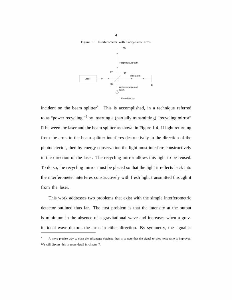
initial LIGO detectorsthe Fabry-Perotresonators(or “arm cavities”) are formed
by insertingpartially transmitting“front” mirrors PF and IF betweenthe beam
splitter and the back mirrors, as shownin Figure 1.3. Sucha cavity is said to
be resonantwhen light enteringthrough the partially transmitting front mirror
interferesconstructivelywith light traveling backand forth inside the resonator.
Nearresonancethephaseof thelight returningfrom theresonatoris very sensitive
to the lengthof the resonator,and the effect of the small displacementproduced
by a gravitationalwaveon the intensity at the output is magnified.
Larger signals can also be obtained by increasingthe amount of power
4
Figure 1.3 Interferometerwith Fabry-Perotarms.
LaserInline arm
Perpendicular arm
PB
IBBS
Photodetector
Antisymmetric port(dark)
PF IF
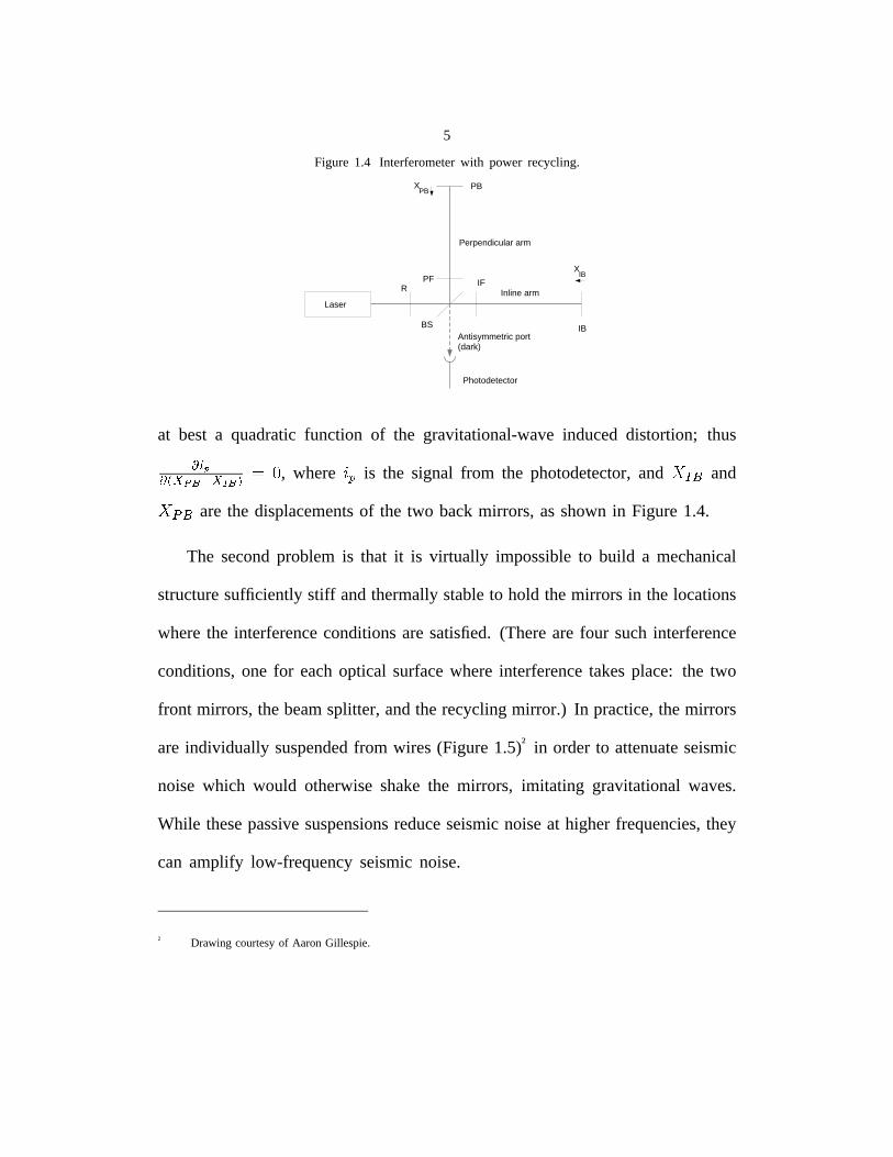
incident on the beam splitter*. This is accomplished,in a techniquereferred
to as“power recycling,”6 by insertinga (partially transmitting)“recycling mirror”
R betweenthelaserandthebeamsplitterasshownin Figure1.4. If light returning
from the armsto the beamsplitter interferesdestructivelyin the directionof the
photodetector,thenby energy conservationthe light mustinterfereconstructively
in the directionof the laser. The recyclingmirror allows this light to be reused.
To do so,therecyclingmirror mustbeplacedsothat the light it reflectsbackinto
the interferometerinterferesconstructivelywith freshlight transmittedthroughit
from the laser.
This work addressestwo problemsthat exist with the simple interferometric
detectoroutlined thus far. The first problem is that the intensity at the output
is minimum in the absenceof a gravitationalwave and increaseswhen a grav-
itational wave distorts the arms in either direction. By symmetry,the signal is
* A morepreciseway to statethe advantageobtainedthus is to note that the signal to shotnoiseratio is improved.
We will discussthis in moredetail in chapter7.
5
Figure 1.4 Interferometerwith power recycling.
LaserInline arm
Perpendicular arm
PB
IBBS
Photodetector
Antisymmetric port(dark)
PF IFR
XPB
XIB
at best a quadraticfunction of the gravitational-waveinduceddistortion; thus������������ ������������ , where ��� is the signal from the photodetector,and ����� and
�! � arethe displacementsof the two backmirrors, asshownin Figure1.4.
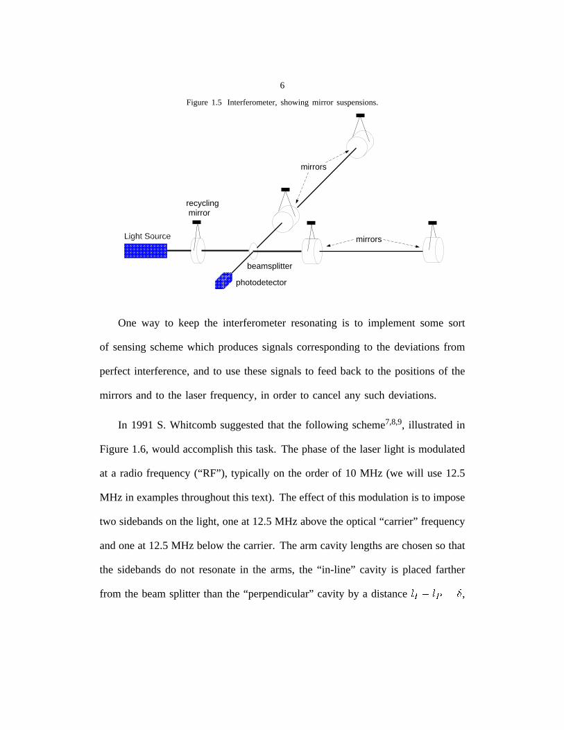
The secondproblemis that it is virtually impossibleto build a mechanical
structuresufficiently stiff andthermallystableto hold themirrors in the locations
wherethe interferenceconditionsaresatisfied.(Thereare four suchinterference
conditions,one for eachoptical surfacewhereinterferencetakesplace: the two
front mirrors, thebeamsplitter,andtherecyclingmirror.) In practice,themirrors
areindividually suspendedfrom wires (Figure1.5)† in orderto attenuateseismic
noise which would otherwiseshakethe mirrors, imitating gravitationalwaves.
While thesepassivesuspensionsreduceseismicnoiseat higherfrequencies,they
can amplify low-frequencyseismicnoise.
† Drawing courtesyof Aaron Gillespie.
6
Figure 1.5 Interferometer, showing mirror suspensions.
mirrors
mirrorsLight Source
beamsplitter
photodetector
recycling mirror
One way to keep the interferometer resonating is to implement some sort
of sensing scheme which produces signals corresponding to the deviations from
perfect interference, and to use these signals to feed back to the positions of the
mirrors and to the laser frequency, in order to cancel any such deviations.
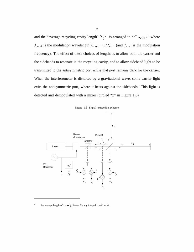
In 1991 S. Whitcomb suggested that the following scheme7,8,9, illustrated in
Figure 1.6, would accomplish this task. The phase of the laser light is modulated
at a radio frequency (“RF”), typically on the order of 10 MHz (we will use 12.5
MHz in examples throughout this text). The effect of this modulation is to impose
two sidebands on the light, one at 12.5 MHz above the optical “carrier” frequency
and one at 12.5 MHz below the carrier. The arm cavity lengths are chosen so that
the sidebands do not resonate in the arms, the “in-line” cavity is placed farther
from the beam splitter than the “perpendicular” cavity by a distance��� �������
,
7
and the “average recycling cavity length”���������� is arranged to be* � ������� where
���� is the modulation wavelength �������� ��� ���� (and � ���� is the modulation
frequency). The effect of these choices of lengths is to allow both the carrier and
the sidebands to resonate in the recycling cavity, and to allow sideband light to be
transmitted to the antisymmetric port while that port remains dark for the carrier.
When the interferometer is distorted by a gravitational wave, some carrier light
exits the antisymmetric port, where it beats against the sidebands. This light is
detected and demodulated with a mixer (circled “x” in Figure 1.6).
Figure 1.6 Signal extraction scheme.
Laser
I Q
IQ
Q
90RFOscillator
Phase Modulation
I
o
L I
l I
l P
L P
v1
v2
v 3v 4
Pickoff
Isolator
* An average length of ��� �! " ! for any integral � will work.
8
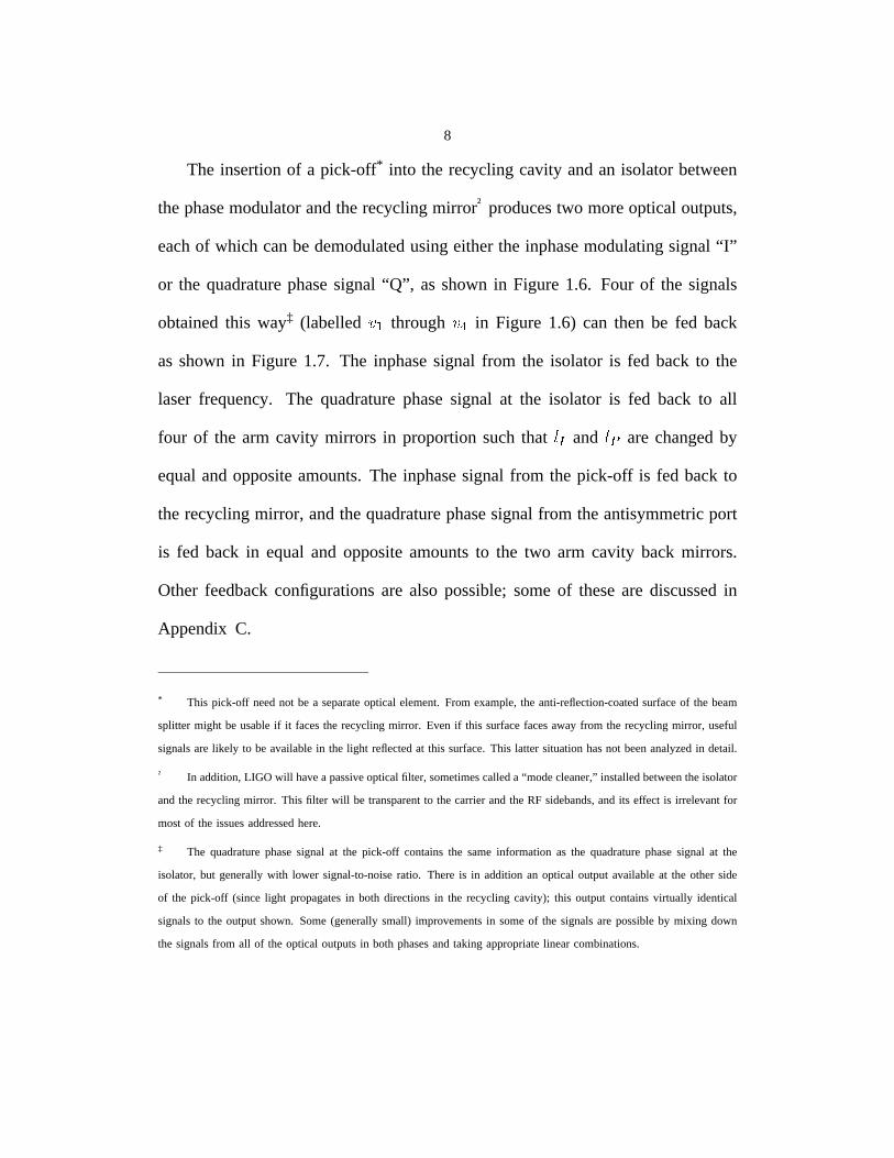
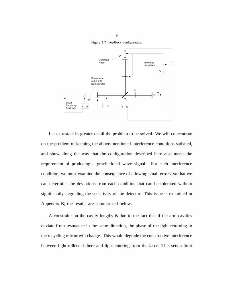
The insertionof a pick-off* into the recyclingcavity andan isolatorbetween
thephasemodulatorandtherecyclingmirror† producestwo moreopticaloutputs,
eachof which canbedemodulatedusingeitherthe inphasemodulatingsignal“I”
or the quadraturephasesignal “Q”, asshownin Figure 1.6. Four of the signals
obtainedthis way‡ (labelled ��� through ��� in Figure 1.6) can then be fed back
as shownin Figure 1.7. The inphasesignal from the isolator is fed back to the
laser frequency. The quadraturephasesignal at the isolator is fed back to all
four of the arm cavity mirrors in proportionsuchthat���
and��
arechangedby
equalandoppositeamounts.The inphasesignal from the pick-off is fed backto
the recyclingmirror, andthequadraturephasesignalfrom theantisymmetricport
is fed back in equaland oppositeamountsto the two arm cavity back mirrors.
Other feedbackconfigurationsare also possible;someof theseare discussedin
Appendix C.
* This pick-off neednot be a separateoptical element.From example,the anti-reflection-coatedsurfaceof the beam
splitter might be usableif it facesthe recyclingmirror. Evenif this surfacefacesawayfrom the recyclingmirror, useful
signalsarelikely to be availablein the light reflectedat this surface.This latter situationhasnot beenanalyzedin detail.
† In addition,LIGO will havea passiveopticalfilter, sometimescalleda “modecleaner,”installedbetweentheisolator
andthe recyclingmirror. This filter will be transparentto the carrierandthe RF sidebands,andits effect is irrelevantfor
mostof the issuesaddressedhere.
‡ The quadraturephasesignal at the pick-off containsthe sameinformation as the quadraturephasesignal at the
isolator,but generallywith lower signal-to-noiseratio. Thereis in addition an optical output availableat the otherside
of the pick-off (sincelight propagatesin both directionsin the recycling cavity); this output containsvirtually identical
signalsto the outputshown. Some(generallysmall) improvementsin someof the signalsare possibleby mixing down
the signalsfrom all of the optical outputsin both phasesandtaking appropriatelinear combinations.
9
Figure 1.7 Feedbackconfiguration.
I Q I QI Q
Photodiode with I & Q Demodulator
Laserfrequencyfeedback
Summing Node Inverting
Amplifiers
Let us restatein greaterdetail the problemto be solved.We will concentrate
on the problemof keepingthe above-mentionedinterferenceconditionssatisfied,
and show along the way that the configurationdescribedhere also meetsthe
requirementof producing a gravitational wave signal. For each interference
condition,we mustexaminetheconsequenceof allowing small errors,so thatwe
can determinethe deviationsfrom eachcondition that can be toleratedwithout
significantly degradingthe sensitivity of the detector.This issueis examinedin
Appendix B; the resultsare summarizedbelow.
A constrainton the cavity lengthsis due to the fact that if the arm cavities
deviatefrom resonancein the samedirection, the phaseof the light returningto
therecyclingmirror will change.Thiswoulddegradetheconstructiveinterference
betweenlight reflectedthereand light enteringfrom the laser. This setsa limit
10
of� ���������
to the common-mode-displacementof the cavity backmirrors,or
equivalently,a limit on the common-modearm cavity phase*
�� ���� ��� ��� ���������������� (1.1)
� is definedas the sum of the arm cavity round-trip phases†:
�� !"�$#&%(')!"�+*,%(1.2)
The condition on the phaseof light returning to the recycling mirror also
constrainsthe common-moderecycling cavity phase,suchthat- ! - #.% ')! - *,%
� �0/1�2� (1.3)
(where- #.%,354"6 %87 # 4 -:9�;8<>=
and- *,%?354"6 %�7 * 4 -:9@;�<>=
).
If the arm cavities deviatefrom resonancein oppositedirections,then the
destructiveinterferenceat the antisymmetricport could be disturbed,allowing
excesslight to hit the photodetector‡. This setsa condition on the differential
* We will seethat using differential and common-modecombinationsof phasesis more convenientthan using the
individual phasesthemselves.
† Theround-tripphaseis thephasechangethe light accumulatesin travelling twice the lengthof thecavity, including
the Guoy phase,which is a phasedeficit due to the fact that the laser beam has a finite diameter. For exampleACBED�FHG�I DKJ B:LMG�N�OEPRQ>S
, whereI D FTGVUXWKY D
is the wave numberof the light. It will generallybe more useful
for us to work with theseround-tripphasesthanwith the distancesbetweenadjacentmirrors. We usethe subscript Z to
identify quantitiesrelatedto the carrier; later we will usethe subscripts[ andL [ for the upperandlower RF sidebands.
‡ Excesslight on the photodetectorrepresentsan unnecessarylossof light from the interferometerwhich reducesthe
optical efficiency andgeneratesadditionalshotnoise.
11
changein arm cavity phases:��� ������� �����
�� ��� ��� (1.4)
The requirementabove, to keep excesslight from the antisymmetricport
photodetector,alsoconstrainsthe differential recyclingcavity phase,suchthat� � � � ��� � � ��
��� ��� ��� (1.5)
In thefollowing chapterswewill investigatethebehaviorof theinterferometer
output signals in responseto motion of the mirrors and changesin the laser
frequency.This detailedcharacterizationis necessaryfor the designandanalysis
of a control system. Thereare two parts to this analysis: an analytic approach
in which approximationsare madeand relatively simple expressionsdescribing
the interferometerresponsearederived,anda numericalapproach,within which
the approximationsare lesssignificantand which thereforecan be usedto test
the validity of the approximationsmadein the analyticderivations.The valueof
the analyticderivationis that it moreclearly expresseshow the choiceof certain
opticalparametersin theinterferometer(suchasmirror reflectivitiesandpositions)
affects critical aspectsof the behaviorof the instrument. For example,we will
seethat if the asymmetry�
is chosento be too large, the responseof � � to���
containsa right-half-plane-zero,which compromisescontrolsystemperformance.
This sort of conclusioncan be derived from numericalmodelsonly through a
tediousexplorationof parameterspaceandthe useof inductiveassumptions.
12
On the other hand, someaccuracyhas beensacrificed in the derivation of
the analytic model. Our goal will be to derive expressionswhich are accurate
to 10% over the rangeof frequenciesin which the servosfeeding back to the
mirror positionsare active. It is for honing thesepredictionsthat the numerical
modelsare useful.
The LIGO interferometersare not yet sufficiently well specifiedto merit a
detailednumericalanalysisandcontrol systemdesign*. Nonetheless,theexercise
of analyzinga possibleinterferometerand designinga control systemfor it is
useful, and will give insight toward a final design. A set of possibleoptical
parametersfor a LIGO interferometeris listed in Table 1.1. We will apply
our analytic resultsand our numericalmodel to this interferometerto explore
its behavior,and then we will designa control systemaroundit, to meet the
specificationslisted above.
It is virtually certainthat neitherthe optical parametersnor the specifications
will remain unchangedbetweenthe time of this writing and the time when a
LIGO control systemis installed, and for this reasonwe will emphasizemore
the methodsof analysisand designthan the detailsof our numericalexample.
The numericalmodel will provide examplesof the size of neglectedquantities
* For example,specificationsfor mirror surfaceerror have not beenset and possibletrade-offs betweencost and
quality arestill beingevaluated.† Thearmcavity lengthsaredisplacedslightly from thelengthwheretheRF sidebandswould beexactlyanti-resonant.Seealso the footnoteon p. 27, andSection7.5.

13
Table 1.1 Possibleoptical parametersfor a LIGO interferometer.
Quantity Symbol Value Units
Recyclingmirror
���5%
Arm cavityfront mirrors
���3%
Arm cavityBack mirrors
�����Mirror(power)transmissions
BeamSplitter
� ���50%- /2
Pick-off reflectivity �� 0.1%
Loss in eachoptical element 100 ppm
In-line cavity �� 4002.004† metersArm cavitylength Perpen-
dicular cavity� 4001.996 meters
recyclingmirror toin-line cavity
� � 6.29 meters
Recyclingcavity lengths recycling
mirror toperpen-dicular cavity
� 5.71 meters
Laserpower��� � ����� ������� photons/
second
Modulation index 0.1 radians
ModulationFrequency ! 12.5 MHz
comparedto relevant ones, and will give us some idea of the magnitudeof
the errors introducedby the approximationsmadewithin the analytic approach.
It is hopedthat, as the parametersand specificationsof LIGO interferometers

14
becomebetterdefined,thesesamemethodswill be valuabletools for designing
and analyzing control systems,and may even influence the choice of optical
parametersand the definition of performancespecifications.
15
Chapter 2 DC Analysis
We begin our analysisof the interferometerby obtainingthe derivativesof
the voltages ��� with respectto the mirror positions.‡
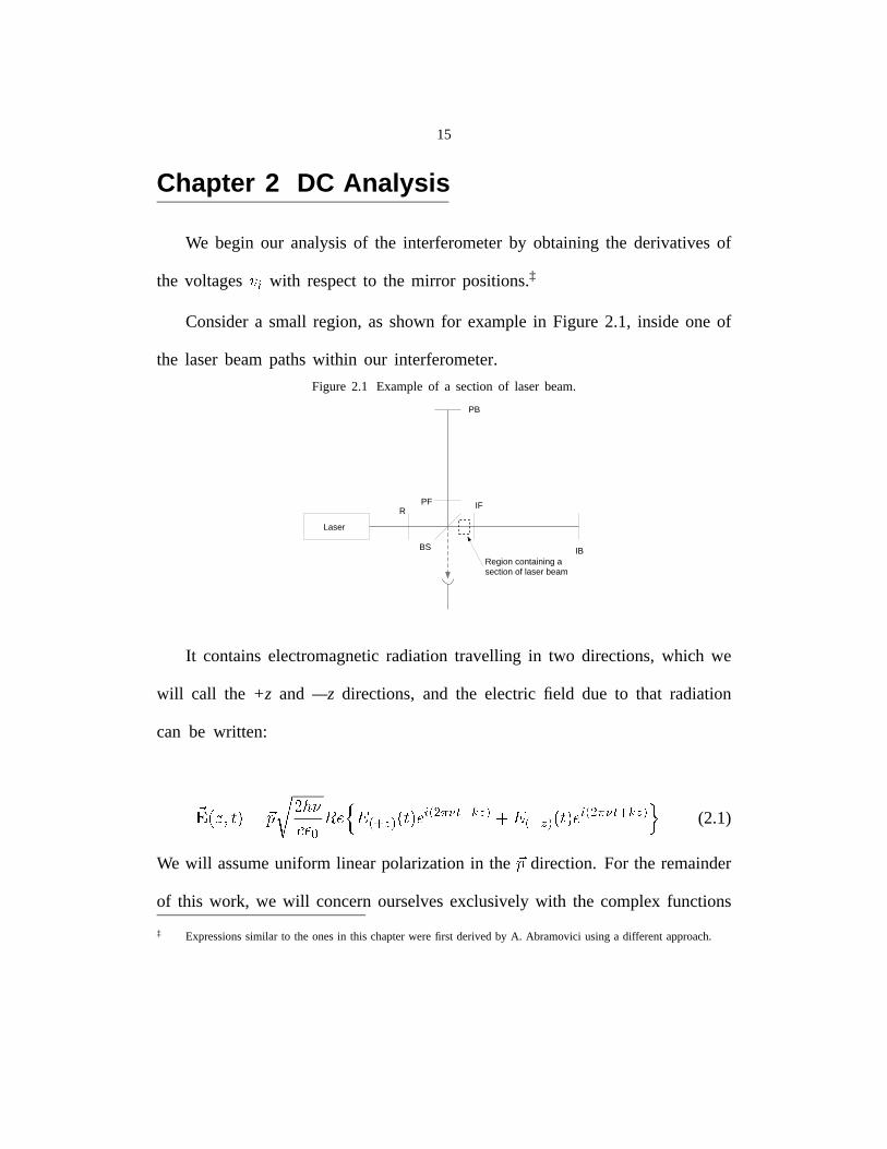
Considera small region,as shownfor examplein Figure 2.1, inside one of
the laserbeampathswithin our interferometer.
Figure 2.1 Exampleof a sectionof laser beam.
Laser
PB
IBBS
PF IFR
Region containing a section of laser beam
It containselectromagneticradiation travelling in two directions,which we
will call the +z and —z directions,and the electric field due to that radiation
can be written:
��������� �� �� �������������� �!#"%$�& �'�� �� !)(+*-,/.�0�12$�&43 5!607$�& �'�� �
� !#(�*�,/.'"812$�& (2.1)
We will assumeuniform linear polarizationin the�� direction. For the remainder
of this work, we will concernourselvesexclusivelywith the complexfunctions
‡ Expressionssimilar to the onesin this chapterwerefirst derivedby A. Abramovici usinga differentapproach.
16
of time�������������
and���� ��������
, which we will refer to asthe field travelingin the
+z direction and the field traveling in the –z direction, respectively.The factor���������� is usedto make the units of the fields ��� �����! #"%$ (the field magnitude
squaredequalsthe numberof photonsper second),which is convenientwhen
calculatingshot noise.
The light from the laser is phasemodulatedat someangular frequency &beforeenteringthe interferometer.This meansthat10 if
�('is the field from the
laserand�*),+ � is the field incident on the interferometer,
�*),+ �.- � '�/ )10�243�57698:<;=?>@��� 'BADC :BE�F>@��� ' / )�698 AGC :BEH4>@��� ' / ),6I8
�()�+ � ; A �*),+ � E / )�698 A �(),+ � E / ),698(2.2)
we call�(),+ � ; the carrier field, and
�(),+ � E and�*),+ � E the upper RF sideband
field and the lower RF sidebandfield, respectively. We will continue to use
numeral subscriptsto index different frequencycomponentsof the light, and
literal subscriptsto denotelocation.
In theremainderof this chapter,wewill first showhowthefieldsincidentona
photodetectoraffect thecorrespondingmixeroutputandhow thederivativesof the
mixer outputarerelatedto thederivativesof thosefields. Thenwe will analyzea
simpleFabry-Perotcavity to find thefieldsandtheir derivativeswithin thecavity.
Finally we will solvefor thefields in the interferometerandtheir derivatives,and
17
concludewith expressionsfor thederivativesof themixer outputswith respectto
thephases�������������
, and���
. Thesearetheneasilyinterpretedasthe response
in the mixer outputsto changesin mirror positionor laserfrequency.
2.1 Photodetector, Mixer
If we assumethat the photodetectorshaveunit quantumefficiency then the
photocurrentin a detectoris
�� �� � �� ��������������� �!��� � �� � �"�#� �
� � � � � � � � � � � � � �%$'&�� � � �)(� � � � �"�#���$*&+� � (� � � � ��� (� � � ���"�#�
(2.3)
We assumethat the mixersaredouble-balancedmixers,followed by low-passor
notchfilters to eliminateharmonicsof themodulationfrequency.To a reasonable
approximation§, the mixer multiplies its input by ,.-0/21�3 (or /5476�1�3 if the mixer is
fed by the quadraturephaselocal oscillatorsignal). By the Fouriershift theorem
(or “heterodyne”theorem11), the only frequencycomponentsof the photocurrent
which will passthroughthe low-passfilter unattenuatedare at frequenciesnear
§ The true effect of mostmixers is to multiply by somethingmoreclosely resemblinga squarewave. This haslittle
effect if themodulationindex is smallor if thephotodiodeis tuned,with a resonantfilter, to besensitiveonly to amplitude
modulationat frequenciesnearthe modulationfrequency.
18
�. The inphaselow-passfilter output then is
��������� � �
���������� ������ ��� �!���� � � �#"%$ �'& (*)�+ � �-,/.0�-,
�1� ������ ��� �2�3�� � �(2.4)
wherefor conveniencewe havemodelledthelow passfilter asa devicewhich
averagesover an integral numberof modulationperiods 465$ .
Similarly,
�879�:�;�< =�> ������ ���?�2�3�� � � (2.5)
Note that for pure phasemodulation, for exampleif� � "A@CB , both outputs
vanish: �D�EF�87GIH .Now we canfind the rateof changeof thesemixer outputs.Suppose
���,� � ,
and� �J� are all functionsof someparameterK ; then
L �D�L K
�1� L ���L K
� � � �!� �J� � � �!���LL K� � � �2� ��� � � (2.6)
In the specialcasewhere� � � �J� and both are pure imaginaryand their
derivativesarerealandequal,and���
is realandits derivativeimaginary,we have
L ���L K
�CMN����� � �� MN��� �L �9�L K
�� MN� � �L � �L K (2.7)
Recognizing�"PORQRS O QSDT as the rate of changeof the phaseof
��U, we seethat
in this specialsituation SDV;WSXT is proportionalto the differencebetweenthe rateof
changeof carrier phaseand the rateof changeof sidebandphase.
19
Similarly
������������
�� ������� �� ����������� �� �
��� � �� ������ �(2.8)
and if ��
and ����
areequalandpure imaginary,and if !�
is real, we have
�"������#� � $�
����%� � ��� � �
(2.9)
We seethat a quadraturephasesignal is producedif onesidebandgrowsandthe
other shrinks.
2.2 Fields in Optical Cavities
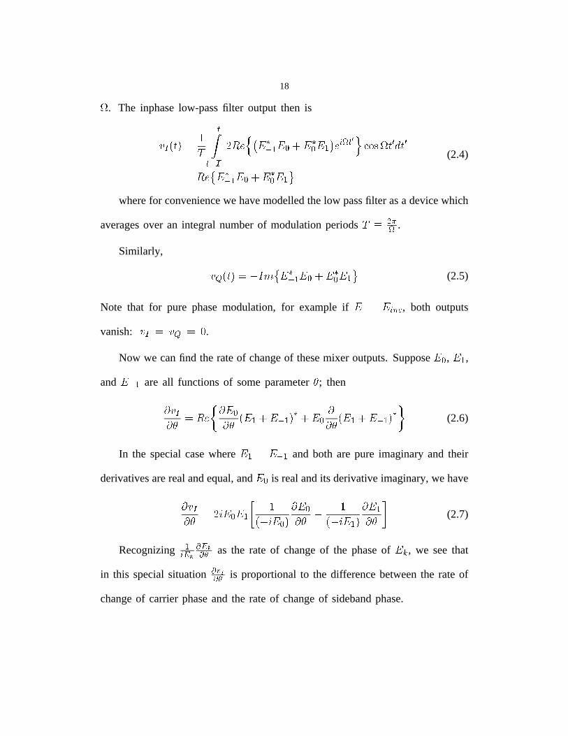
Now let us showhow the fields are relatedto the mirror positions.
Figure 2.2 Partially transmittingmirror.
AE v
E w
E x
+ -
Laser beam
Considerfirst a partially transmittingmirror A, illuminatedfrom theleft, asin
Figure2.2. Wedefineits reflectivity&(' (sometimescalled“amplitudereflectivity”)
astheratioof thereflectedfield !)
to theincidentfield +*
. Wewill alwaysmodel
our mirrors as having positive real reflectivity on one side, and we denotethat
side with a “+” as shown. We will also model the transmission,�' as being
positiveandreal; thenenergy conservationrequires12 thatwe assignnegativereal
reflectivity to the other side of the mirror, denotedby a “-”.
20
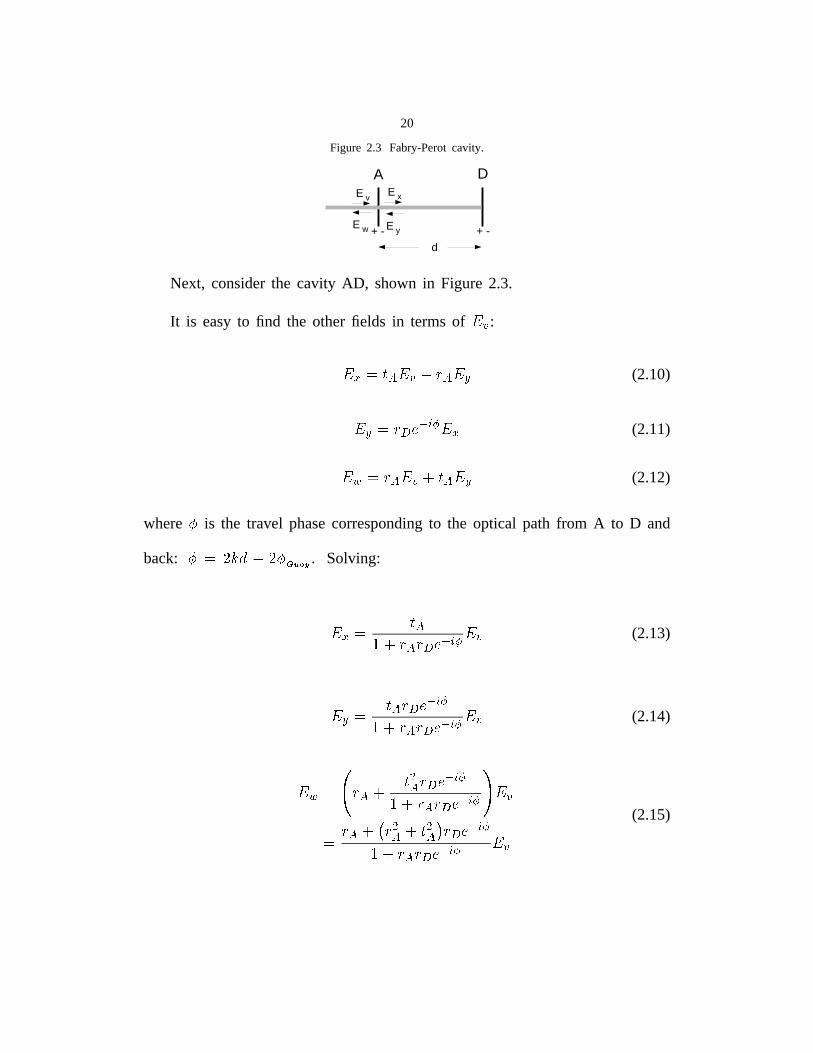
Figure 2.3 Fabry-Perotcavity.
A DE v
E w
E x
E y+ - + -
d
Next, considerthe cavity AD, shownin Figure 2.3.
It is easyto find the other fields in termsof���
:
����������� � ����(2.10)
���������������������(2.11)
�������������� �!����(2.12)
where " is the travel phasecorrespondingto the optical path from A to D and
back: " �$#�%'& # ")(+*-,/. . Solving:
����� �!0 �1� � � � ����� ��� (2.13)
����� �-2�3�4� �5���0 �6� 2���4� ����� ��� (2.14)
����� � � �87 � � � �����0 �6� � � � �5��� ���
� � � � 7 �9� 7 � � � �5���0 �1� :����� �5�;� ���
(2.15)
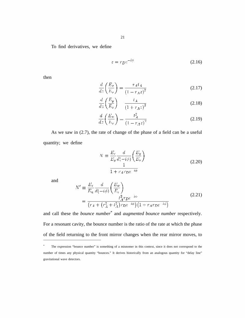
21
To find derivatives,we define
������������ (2.16)
then ���
������ � �������
����� � � � �"! (2.17)���
��#��� � � �
�$�%� � � �&� ! (2.18)�� �
��'��� � � !�
����� � � �&� ! (2.19)
As we sawin (2.7), the rateof changeof the phaseof a field canbe a useful
quantity; we define
( �����#
�� � )+* �
��#���
� ��,� � � � � � ���
(2.20)
and (.- ���� '
�� � )+* �
��'� �
� � !� � � � ��/ � � � � !� � � !� � � � 0�� ��� � � � � � ���
(2.21)
and call thesethe bounce number* and augmented bounce number respectively.
For a resonantcavity, thebouncenumberis theratio of therateat which thephase
of the field returningto the front mirror changeswhenthe rearmirror moves,to
* The expression“bouncenumber” is somethingof a misnomerin this context,sinceit doesnot correspondto the
numberof times any physical quantity “bounces.” It deriveshistorically from an analogousquantity for “delay line”
gravitationalwavedetectors.
22
the rate at which that phasewould changeif the front mirror were absent.The
augmentedbouncenumberis the sameratio exceptthat it is defined for the field
���reflectedfrom the cavity.
2.3 Fields in the Interferometer
We can use theseexpressionsto solve rather easily for the fields in our
interferometerand also for their derivatives. We will first find the carrier fields
everywhere,then the sidebandfields. Thenwe will find the derivativesof these
fields. Finally we will assembletheseinto expressionsfor the derivativesof the
mixer outputs.
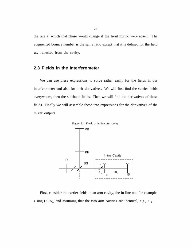
Figure 2.4 Fields at in-line arm cavity.
R
IF IB
PF
PB
BSE a
E b IΦ
Inline Cavity
+ - + -
First, considerthecarrierfields in anarmcavity, the in-line onefor example.
Using (2.15), and assumingthat the two arm cavitiesare identical, e.g., ������
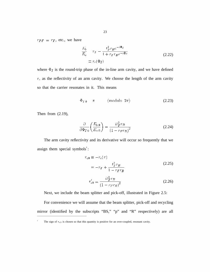
23
����� ��� , etc., we have
������ � ��� ��� �������������
� � ����� � � ����������! #"%$'&
(2.22)
where " $ is the round-tripphaseof the in-line arm cavity, andwe havedefined
��� as the reflectivity of an arm cavity. We choosethe length of the arm cavity
so that the carrier resonatesin it. This means
" $)( +* -,/.1032145.76 * & (2.23)
Then from (2.19),
88 "�$�(
� � (�9� (
: � � ��� � � � � � & � (2.24)
The arm cavity reflectivity andits derivativewill occurso frequentlythat we
assignthem specialsymbols†:
��� ( ���; * &
� ��� ��� � �� � � ���
(2.25)
�=<� (: �� ���
� ����� � & � (2.26)
Next, we includethe beamsplitter andpick-off, illustratedin Figure2.5:
For conveniencewe will assumethat thebeamsplitter,pick-off andrecycling
mirror (identified by the subscripts“BS,” “p” and “R” respectively)are all
† The sign of >@?�A is chosenso that this quantity is positivefor an over-coupled,resonantcavity.
24
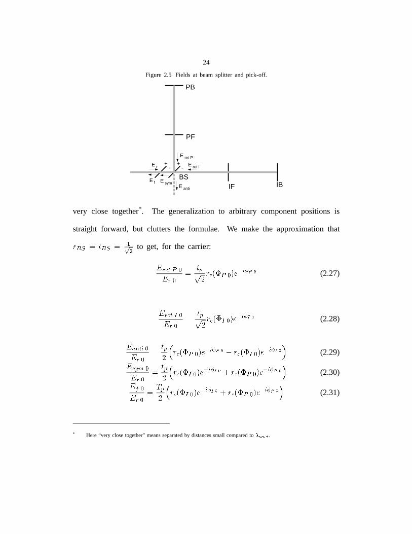
Figure 2.5 Fields at beam splitter and pick-off.
IF IB
PF
PB
E r
E symE anti
E f
E ret P
E ret I+
-+
-
BS
very close together*. The generalization to arbitrary component positions is
straight forward, but clutters the formulae. We make the approximation that
������������� � � to get, for the carrier:
������������ ��� � ���
� ��� �"! �#��$�%'&)(+*�,.-(2.27)
� ���/�10��� ��� � � �
� ��� �"! 02� $�% &)(3*�45-(2.28)
�7698 � ( �� �:� � � �� ��� �"! �#� $;% &)(+*�,<- �=�9�>! 02� $�% &)(+*=4'-
(2.29)��?"@BA �� �:� � � �
� ���9�>! 02��$;%C&)(3*=4C-ED ��� �>! �F�=$�%C&)(+*�,<-(2.30)
�HG �� ��� �JI �� ���9�>! 02��$;% &)(3*=4C- D �=�9�>! �F��$;% &)(3*�,E-
(2.31)
* Here “very close together” means separated by distances small compared to KBLNMPO .
25
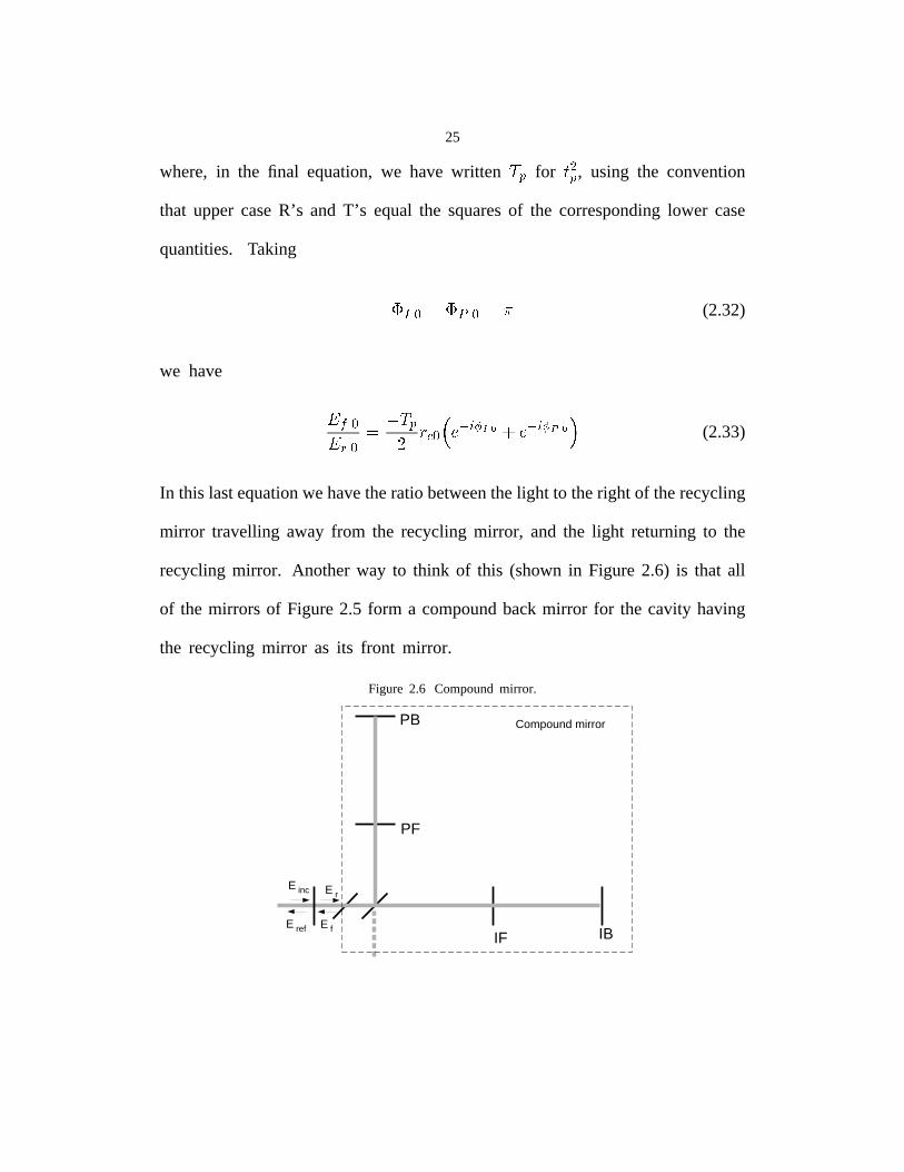
where, in the final equation,we have written���
for ���, using the convention
that uppercaseR’s and T’s equal the squaresof the correspondinglower case
quantities. Taking
�������� �����(2.32)
we have
��� ���� � ���
����� � � �"!$#&%('*)+�,�"!-#/.0'(2.33)
In this lastequationwehavetheratiobetweenthelight to theright of therecycling
mirror travelling away from the recycling mirror, and the light returning to the
recycling mirror. Another way to think of this (shownin Figure 2.6) is that all
of the mirrors of Figure2.5 form a compoundbackmirror for the cavity having
the recycling mirror as its front mirror.
Figure 2.6 Compoundmirror.
IF IB
PF
PB
E r
E f
Compound mirror
E inc
E ref
26
Using (2.13) we have
��������������
��� � ����� � ������ ��� ��� ��!#" �� ��� $%! (2.34)
and to achievemaximum power buildup in the recycling cavity,† we need to
arrangefor the secondterm in the denominatorto be asnearlyaspossibleequal
�. Hencewe choose
&(' � � &*) � �,+ (2.35)
so that
���-��.����(� �
�� � �/�0� � ��� (2.36)
Using (2.14) and (2.15)
�21 ��.����(�3�
4� �0� � ���� � � �0� � ��� (2.37)
� ��5 1 �������(� � � � �� �0� � ���
� � � �0� � ���� � �0� � ���� � � �6� � ���
(2.38)
wherethe last expressionwasderivedusingthe approximationthat lossesin the
recycling mirror can be neglected‡:� �� " � � �
.
† The ratio 778
is calledthe recycling gain or the recycling factor andis a measureof the benefitdeliveredby
the recyclingmirror.
‡ Lossesof a few tensof partsper million areanticipatedin the recyclingmirror, whereasthe total round-triplossin
the recyclingcavity is expectedto be a few percent.
27
Since����������� ���
,
���������������� � ����������� �
! �"��#$�%�"� � (2.39)
and from (2.29)
��&��"'(�)�*�,+(2.40)
Now we turn to the sidebandfields in an arm cavity. We begin with the
uppersideband;the derivation for the lower sidebandis almost identical. The
armcavity lengthis chosensothat thesidebandsarealmostexactlyantiresonant§,
i.e. -/.10 +. Referringback to Fig. 2.4,
�"� 0�32 0��& 0
�4�"576 ��85 �"9! 6:��5;� 9
(2.41)
and �)<� 0=
= -/.10� 2 0��& 0
� > � 85 � 9? ! 6:� 5 � 9A@ 8
(2.42)
Becausethe sidebandsare nearly perfectly excludedfrom the arm cavities,
we canapproximatethe expressionsaboveas beingunity andzero, respectively
(in our numericalexample,their valuesare 0.99995and 0.008).
§ If they wereexactly antiresonantthen the RF sidebandsat BCED would all be resonant,causingthe interferometer
responseto be very sensitiveto arm cavity lengthandmodulationdepth.SeealsoSection7.5.
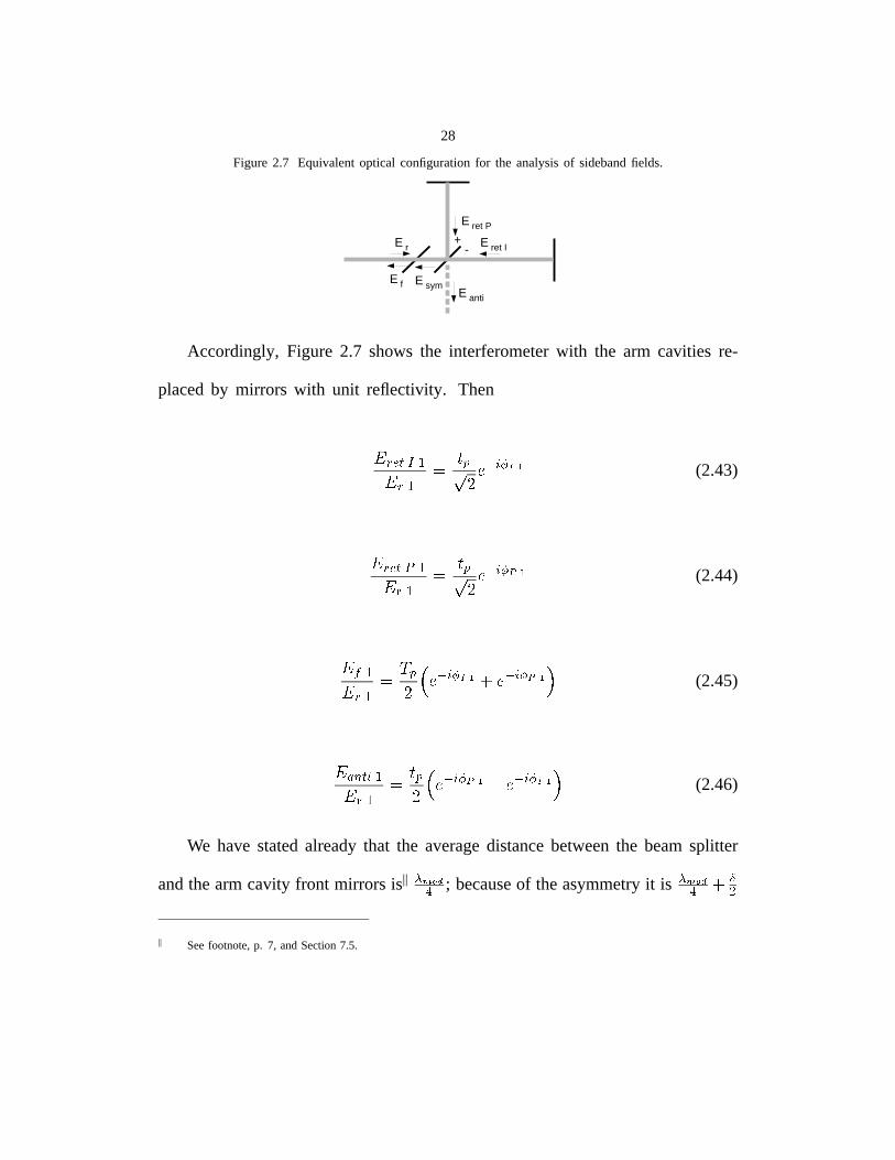
28
Figure 2.7 Equivalentoptical configurationfor the analysisof sidebandfields.
E r
E symE anti
E f
E ret P
E ret I+
-
Accordingly, Figure 2.7 showsthe interferometerwith the arm cavities re-
placedby mirrors with unit reflectivity. Then
���������� �� �
�������
�������(2.43)
����������� �� �
��� � �
� ��! �(2.44)
�#" � ��$�
% �� � �
� �����'&� �
� � ! �(2.45)
��(*) � � � �� �
+�� ���
� � ! ��,�
�����-�(2.46)
We havestatedalreadythat the averagedistancebetweenthe beamsplitter
andthearmcavity front mirrors is|| .0/21+34 ; becauseof theasymmetryit is .5/21+34 &768
|| Seefootnote,p. 7, andSection7.5.
29
for the in-line arm and�������� � for the perpendiculararm. Then
��� ���� ����������
�����! " �$#�
�% �'& � �(��
� ���) " �$#�
�*�+�-,(2.47)
where, . �/ .
In similar fashiononecanshowthat102 ��3� ,
. It thenfollows that46587 � 4:9 � ;=<�>@?BA�,
(2.48)
4DCFE�GIH 4D9 � J=;�<KAMLOND,
(2.49)
Similarly 4 587 �QP 4:9 P � ;�<R>F?BA�,
(2.50)4DCSE�GTH P 4D9 P �3J=;�<KAULOND,
(2.51)
Finally, as we did for the carrier, we find the sidebandfields everywhereby
consideringthepick-off andeverythingto its right asa compoundmirror (shown
in Figure2.8). The difference�V,
between �K
and 0W
affectsthe transmission
(to theantisymmetricport)of thismirror. Theaverageof��K
and10W
determines
whetherthe cavity formed by the compoundmirror and the recycling mirror is
resonant.
From (2.13) through (2.15):4:9 4DHOE /
� ;MXY Z X\[]<�>F?BA�, (2.52)
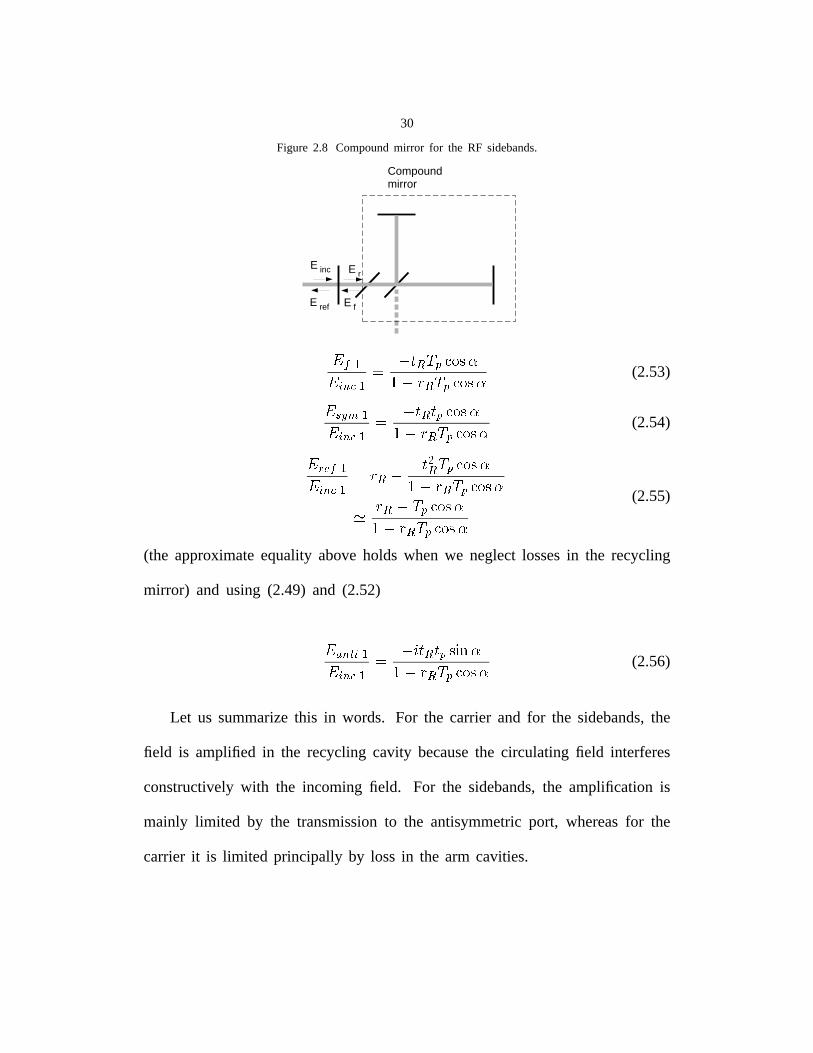
30
Figure 2.8 Compoundmirror for the RF sidebands.
E r
E f
Compound mirror
E inc
E ref
���������� ���
��������������� � ������� �!��� (2.53)
��"$#&% ����'�( �)�
��* +���,���-�� � � ���.�,����� (2.54)
��/�0 ������'�( �1� � �
32� ����� �!�-�� � �4����� �!���
� � �����,���-�� � �����.�,���-�
(2.55)
(the approximateequality aboveholds when we neglectlossesin the recycling
mirror) and using (2.49) and (2.52)
��5 �768� ����'�( �9�
: ;�� <�.��=?>��� � �@���.�,���-� (2.56)
Let us summarizethis in words. For the carrier and for the sidebands,the
field is amplified in the recycling cavity becausethe circulating field interferes
constructivelywith the incoming field. For the sidebands,the amplification is
mainly limited by the transmissionto the antisymmetricport, whereasfor the
carrier it is limited principally by loss in the arm cavities.
31
2.4 Derivatives of Mixer Outputs
Now we candifferentiatethefields andfind thederivativesof mixer outputs.
We will considerfirst the differentialsignals: the derivativesof the gravitational
waveoutput ��� andtheisolatorquadratureoutput ��� with respectto phasechanges
���and � � . Then we will calculatethe common-modesignals: the derivatives
of thepick-off andisolatorinphaseoutputs�� and �� with respectto� �
and � � .First we note that since
� ������������ ������������ ��� � ���� � ��� ����� (2.57)
we have �� � � �� � ���� � �
�� � ��� �� � � �� � �
�� � � �� ��
�� � ����� � � � (2.58)
and that for ! constantand ! "� � � � �$# � �&% "' � ! ' � �)(+*&,.-� � ����� ��# � ! '
(2.59)
so that �� � ��� �/� � (2.60)
whetherthe independentvariable is " or# �
.
32
Differential Signals
We beginwith the gravitationalwavesignal. Dif ferentiating(2.29)
������������� �� �
������������� �� �
�� � ��� ����
�������������� �� �
�� � ��� ��
��� ������ "!$#&%' �
(2.61)
and, using (2.8), we have(at the antisymmetricport)
�)(�*�� �� �,+�-
�������������� �� . ��������0/ ��������1��/�243
� �65798 � .;: 2 8 / .<: 2< =!�������>� ' �
�������0/��?� ' /
# %' �(2.62)
which can be further expandedusing (2.49) and (2.51). Equation (2.62) can
be understoodas follows. When �
deviatesfrom @ we ceaseto haveperfect
destructiveinterferenceat the antisymmetricport for the carrier. The sizeof this
deviationfrom perfectdestructiveinterferenceis proportionalto the rate# %' � at
which thecarrierfield returningto thebeamsplitter from thearmcavitieschanges
with ��
. This carrier light then beatsagainstthe sidebandswhich are present
becauseof the asymmetry,producingmodulationof the photocurrentat A , and
a signal at the mixer output.
A similar mechanismis responsiblefor the sensitivity to B � at the antisym-
metric port. When B � deviatesfrom 0 we alsoceaseto haveperfectdestructive
interferenceat the antisymmetricport for the carrier. Quantitatively,to find C�DFECHG�I ,
again differentiate(2.29)
33
������������� ��������������������� � � �
�"!$#&% ��"'(#�)*! ��"!+#&% � ,.-�/ % � (2.63)
We now move on to 0�132054&6 . From (2.45) the reflectivity of the compound
mirror for the upper sidebandis 7 -98�:<; �>=@? ����A�B � ; using (2.19) with C 7 -D8�:�; �.=@? ����A<B � we have
������ � �FEHG �
�"!$#&% � , I 7 -J;LK$M =B �FN / I 7 -O8�:�; =O� (2.64)
Similarly, ������ � �PEQG � �
�"!$#&% � � , I 7 -R;FK$M =B �FN / I 7 -98�:�; =O� (2.65)
Sincethe conditionsleadingto (2.9) are satisfied,we have
����S����� �� � �����������T������� � �PE3G ��"!$#&% � , I 7 - ;LK$M =�FN / I 7 - 8�:�; =O�
(2.66)
which can be further expandedusing (2.38).
In words, this sensitivity in��S
to���
is due to the fact that when���
changes,the reflectivity of the compoundmirror increasesfor one RF sideband
and decreasesfor the other. This causesa correspondingchangein the relative
size of the sidebandsreflectedfrom the recycling mirror and a signal according
to (2.9).
Thereis alsoa small dependencein��S
on U � . Becausethe derivative(2.42)
of thearmcavity reflectivity for thesidebandis not exactly V , it is non-negligible
34
whenit is responsiblefor theonly contributionto thesignal. We re-insert�����������and ��� ����� into (2.45) and differentiateto get (using (2.9))
������ ����� ���� ����! �" ��#$ ��#% �'&)(+* "�-,/. � "
0 �1$24365)798-:�<; � 1 243�=?>@5A: � (2.67)
Common-mode Signals
Now let us look at thecommon-modesignals.We beginwith� � , the inphase
pick-off signal. Using (2.31) and (2.18) with
B ��C* "� & " (2.68)
to find DDFEAGHJILKH�MON)P K we have:
�� �RQ
�-S+T�U "�-,V. � " �
0 1 0 3 � �� "W �X; � 1 2Y3 �F� " � (2.69)
Then, using (2.7), we obtain
��� �� �RQZ� �[��A \" ��#% ��#%^] 3 � S+T�U "�-,V. � "
� S�T?U �',V. � _ "
� �� "��� " (2.70)
which canbe further expandedusing(2.25), (2.26),(2.39)and(2.54),andwhere
_ " �;
� S+T�U "� � S+T�U "�a` Q
�;Hcbedgf KH�MhNXP K
��a` Q
� S�T?U "�',V. � "
�;
; �F1 2Y3 �F� "
(2.71)
is thebouncenumberfor the carrierin the recyclingcavity. In words: When � Qchanges,the phaseof the carrier light changesin proportionto the factors i &kjP K i& P K
35
(which is just theaugmentedbouncenumberfor thecarrierin anarmcavity) and
���, generatinga signal accordingto (2.7).
When ��� changes,the phasesof the carrierandof the sidebandsall change,
so that by (2.7) the signal is proportionalto the differencein the ratesof change
of thesephases.To find �������� we have,using (2.31) and (2.45),
�� ����� ������������� � � (2.72)
for the carrier and
�� �!��� �����"�����$#&%('*) (2.73)
for the sidebands;then using (2.18) and (2.7), we have
+-,�+ �-� �/. �021 �(35476 1�8 39476;: � .=<9>@? �
. �BA � �.C<;>D? 8. �BA � 8FE �G� � 8IH (2.74)
where
� 8 � JJ � K7���L#�%('*) (2.75)
�G�and
� 8 arethebouncenumberfor thecarrieranduppersideband(respectively)
in the recycling cavity. The bouncenumberfor the lower sidebandequalsthe
bouncenumberfor the uppersideband.
We now move on to, 8 , the inphasesignal at the isolator. This signal is
producedby thesamemechanismas ���I�NM2� exceptthat therateof changeof carrier
phaseis proportionalto�PO�
insteadof���
. � �@Q�NM2� is found using (2.31), (2.21),
36
(2.19), and (2.7):
������
����� �������� � �
������������� � "!�# � � �$�%� � �'& � (2.76)
�)(�*�+� � � � �,.- � !0/ & - * !1/ &
�����2����3��� �
����� *���3��� * 4 �� � �� �
� � � (2.77)
To find 576985;:7< we use(2.31), (2.19), (2.45), and (2.7):
� (�*�>=?�@� � �, - � !1/ & - * !1/ &
�A����2��A�3��� �
�A���� *�A�3��� * 4 �� 4 �*
(2.78)
Herethemechanismis thesameastheonefor 576CB5;:7< , exceptthatagain,augmented
bouncenumbersare used. With the approximationthat the recycling mirror is
lossless,we can write
4 �� �#
D ����� �� �����2��>=?�
������$�E� � �
! � � �$�%� � �;& !F# � � ���%� � �7&(2.79)
and
4 �* �#
D ����C *� ����C *�>=?�
���� �$��GIH%JLK
! � � �$��GIH%JLK & !�# � � ��� GMH�JLK &(2.80)
Both (2.77) and (2.78) can be expandedusing (2.38) and (2.55).
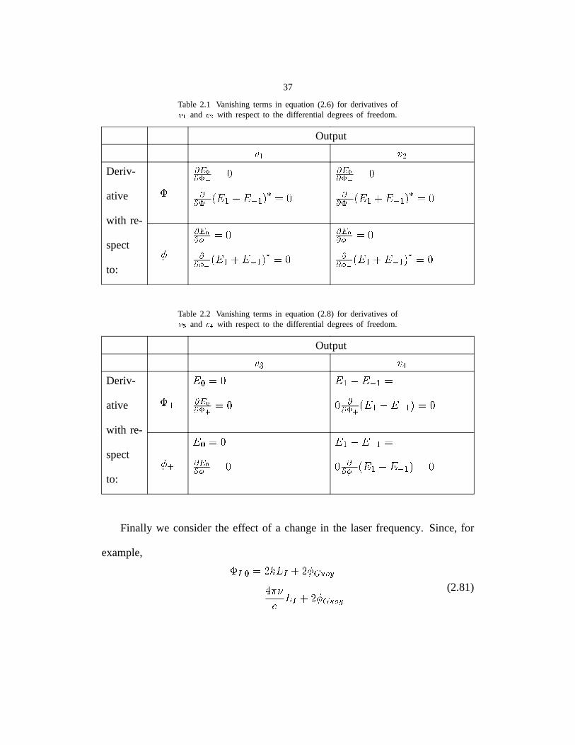
This completesour analysisof the signalsof interest.Onecanshowthat the
remainingeightderivativesall vanish.Table2.1showsthefactorswhichvanishto
make(2.6)vanish,andTable2.3showsthefactorswhich cause(2.8) to vanish.
37
Table 2.1 Vanishing terms in equation (2.6) for derivatives of��� and ��� with respect to the differential degrees of freedom.
Output��� ��Deriv-
ative
with re-
spect
to:
�� ���� �������� �������� ��� � � �! #" �$�
��%� �������� ����&�'� �(� � � �! #" �$�
) � *� � �+� ��� �+� ��� �,� � � �! " ���
*� � �+� ��� �+� �-� �(� � � �! " ���
Table 2.2 Vanishing terms in equation (2.8) for derivatives of��. and �0/ with respect to the differential degrees of freedom.
Output�1 �32Deriv-
ative
with re-
spect
to:
54�76��$� �� � ���8 ���
� � � � � �� *��8 �'� � � � �! ���
) 4�76��$� *� � �+*8 ���
� � � � � �� *+*8 �'� � � � � ���
Finally we consider the effect of a change in the laser frequency. Since, for
example, :9 6 �$;=<?> 9 � ; )�@BA*C#D�FEG,HI > 9 � ; ) @BA*C#D (2.81)
38
changes in this phase can be effected either by a change in the length of the in-line
arm cavity or by a change in the laser frequency. Now
�������� �
���� (2.82)
and �� ����� �
������ (2.83)
so that, for example
�������� �
����������
�������� �
������� ��
�� �����
����
���������� � � ������� ��
�����
����������
(2.84)
where we can make the approximation in the last line because�
and because������ ! ��"���#$! . Similarly, we will use
���&%���
����
���'%����� (2.85)
which is a very good approximation for the same reasons.
In chapter 4 we will compare, for our numerical example, the values of the
derivatives found using this analysis and the values found by a numerical model
which makes fewer approximations.
It is easy to generalize the analysis above, of the response to particular
combinations of mirror displacements, to the case of arbitrary combinations. We
39
simply note that the following combinations of mirror displacements and changes
in laser frequency produce no signal at all. They are in the kernel of the Jacobian
of interferometer outputs with respect to mirror position and optical frequency.
1. Displacement of the entire interferometer towards (or away from) the laser.
2. Displacement of the arm cavities towards the beam splitter and displacement
of the recycling mirror away from the beam splitter, all by equal amounts.
3. A change���
in the laser frequency, together with displacements of the
arm cavity input mirrors PF and IF away from the recycling mirror, through
distances ��� ���� and � ���� , and displacements of the arm cavity back mirrors
PB and IB through distances of � � ��� � ��� ���� and � � �� � �� ���� respectively.
These three combinations have the property that they leave the relative phases of
any interfering beams unchanged.
From this observation we can conclude, for example, that a displacement of
the recycling mirror towards the beam splitter will generate the same signals as
an equal-sized displacement of all of the arm cavity mirrors towards the beam
splitter, since the two differ by an element (#2 above) of the kernel. Similarly,
displacement of the beam splitter and of the recycling mirror, such that � and � �change by equal and opposite amounts, differs only by an element of the kernel
from a displacement of the two arm cavities in opposite directions in the same
amounts, and the two combinations must produce the same signal.
40
Chapter 3 InterferometerFrequency Response
Implicit in the analysisof the last chapter,sincewe did not allow any of the
fields���
,���
, or�����
to dependon time, is the assumptionthat changesin the
phases� and occur slowly. Supposeinsteadthat we want to know what the
responsein the output signalsis when the laser frequencychangesabruptly, or
whena mirror vibratesat a high frequency.This is the problemwe will analyze
here.
3.1 Fabry-Perot Cavity
As in Chapter2 we will begin by analyzinga single cavity in somedetail,
andthenextendingthe resultsto the completeinterferometer.The responseof a
Fabry-Perotcavity to backmirror motionhasbeenunderstoodfor sometime13,14,
but we will re-deriveit becauseour methodwill includetheRF phasemodulation
in a naturalway andwill be easilygeneralizedto morecomplexoptical systems.
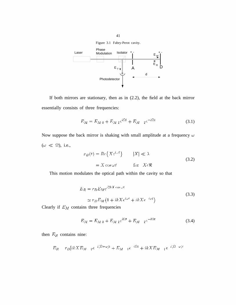
Our cavity, shownin Figure3.1, consistsof two mirrors A andD, separatedby a
distance suchthat the carrier resonatesin the cavity but the two RF sidebands
do not.
41
Figure 3.1 Fabry-Perotcavity.
A DE T
E M
E R
LaserPhaseModulation Isolator
Photodetector
+ - + -
d
If both mirrors are stationary,then as in (2.2), the field at the back mirror
essentiallyconsistsof three frequencies:
���������������� ���������������� �� � �����(3.1)
Now supposethe back mirror is shakingwith small amplitudeat a frequency�( � � ), i.e.,
� �"!$#�% ��&'� ()� �+*,� ( -�.(0/2143 � # 5 1467()8 (3.2)
This motion modulatesthe optical pathwithin the cavity so that
��9:�.; � ���<�=�?>A@�BDCFEAGH*,�; � ��� IJLKNMO(P�H�Q*,��LKRMS(P� � ��*,� (3.3)
Clearly if� �
containsthree frequencies
� � ��� ��� �� �� � ����� �� ���� � � �����(3.4)
then��9
containsnine:
��9T�.; �"U KRMS()�����V �� � �XW � Y�*[Z+� \������ �� � ������LKRMS(P������ ]� � � W � � *SZ?�
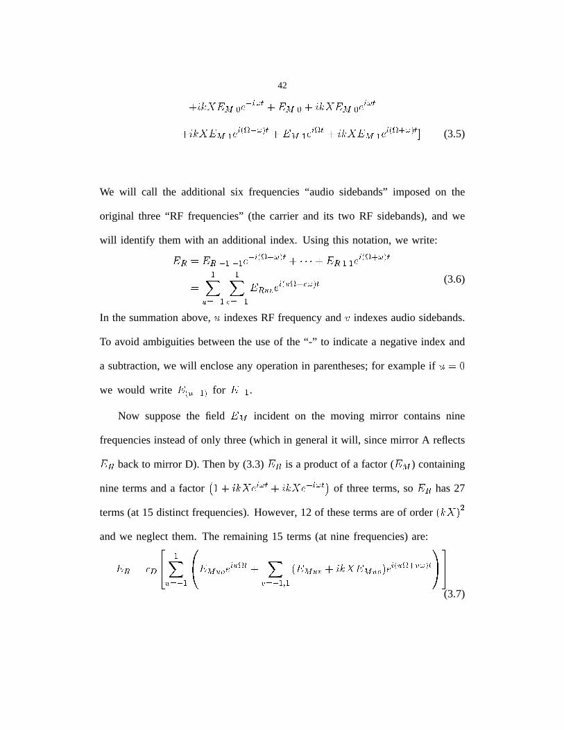
42
������������ ��������������������������� !���"��#������� %$ �'&)(*�+��,-� �.� %$ �)(/� ��������� %$ �0&)(�12��,��43
(3.5)
We will call the additional six frequencies“audio sidebands”imposedon the
original three“RF frequencies”(the carrier and its two RF sidebands),and we
will identify themwith an additionalindex. Using this notation,we write:�576���5 � $ � $ �+�0&�(�12��,-� � ����5 $*$ �'&�(81���,-�
6$
9 : � $$
;<: � $� 5 9�; �0& 9 (81 ; ��,=� (3.6)
In thesummationabove,> indexesRF frequencyand ? indexesaudiosidebands.
To avoid ambiguitiesbetweenthe useof the “-” to indicatea negativeindex and
a subtraction,we will encloseany operationin parentheses;for exampleif > 6�@we would write
� & 9 � $ , for� � $ .
Now supposethe field�
incident on the moving mirror containsnine
frequenciesinsteadof only three(which in generalit will, sincemirror A reflects
�5backto mirror D). Thenby (3.3)
�5is a productof a factor (
� ) containing
nine termsanda factor A �B������ �)�C� �B������ �+���C� of threeterms,so� 5
has27
terms(at 15 distinct frequencies).However,12 of thesetermsareof order D ����E�Fandwe neglectthem. The remaining15 terms(at nine frequencies)are:
� 5 6HG�I$
9J: � $� 9 K � 9 (L� � ;M: � $ONP$ D
� 9�; ��������� 9JK EQ �0& 9 (�1 ; �R,=�(3.7)
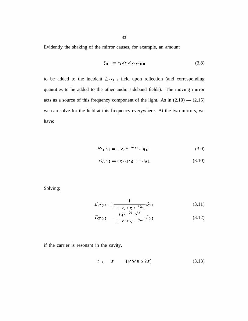
43
Evidently the shakingof the mirror causes,for example,an amount
����� ����� ����� ���(3.8)
to be added to the incident� � ���
field upon reflection (and corresponding
quantitiesto be addedto the other audio sidebandfields). The moving mirror
actsasa sourceof this frequencycomponentof the light. As in (2.10)— (2.15)
we cansolve for the field at this frequencyeverywhere.At the two mirrors, we
have:
��� ����� ������������� !�#" ���(3.9)
� " ��� � � � � � ���%$ �����(3.10)
Solving:
��" ���� && $ � � � � � �'�(� �
�����(3.11)
�) ���� * ��� �'�(���+ -,/.& $ ���0���1� �'�����
�2���(3.12)
if the carrier is resonantin the cavity,
32��� �54 687:9<;+=<>(9@?�4�A(3.13)
44
������������ ��� ���������� ���� ��������� � � �!��
(3.14)
"$#�%'&)(+* � "�#�%',+- (3.15)
"$#.%/& (+*1032 � 4 " #�%',+- 032 (3.16)
Then
576 ��� � 498;: " #�%',+-<0�2= > : >? " #.%',@-�A
���(3.17)
We call the ratio of the audio sidebandfield at the photodetectorto the source
A���
of that field the transmission function B �C� from the shakingmirror to the
optical output and write
5 6 �C� � B �C� A�C�
(3.18)
We find for the lower audio sidebandon the carrier
576 � # � �4D8 : " %',@-E0�2
= > : > ? " %',+-FA� # � (3.19)
Similar expressionscan be found for the other audio sidebands.
Givenfull informationaboutthespectralcontentof5 6
we still needto know
the mixer output when this light is presentat the photodetector.As before,the
photodetectoroutput is
45
��������� � � �
������ �
������ �
� � ��������� ��� �!��"$#�%�
(3.20)
Again, as in (2.3), this containstermsat a numberof frequencies,of which only
thosenear & will bemixeddownto nearDC andpassthroughthe low-passfilter.
Moreover,of thosefrequencies,we areonly interestedin the onesat frequencies
of &('() and & ) becausethesewill bemixeddownto ) , andit is theresponse
in the mixer output at ) that we want*. Thesetermsare
� �+* %$�-,." 0/21 �3
����� �
3
����� ��4�65� �+� � � � ��� � # � ��� � # �7���
�-�!"8#�%
' �95� � � �:� � #� �
� ��� � #;� �7����<� "8#�% �
(3.21)
Then
=�> ���?�+ @A%
%B� �� �C* %$� ,!" �ED F�GIH & �JDLK;�JD
01 �3
����� �
3
�:��� ��B� 5� �� � � � ��� � # � ��� � # '
� � � � ��� � #� 5�
� ��� � #;�� � � "M%
(3.22)
which is in the form
=�> ���?�+01 � N > � � "M% (3.23)
* The only othercomponentpassedby the lowpassfilter is at DC, correspondingto (2.4) and (2.5). We areusually
interestedin the responseto small motionsaroundthe point of perfectresonance,wherethis term vanishes.
46
with
����
�����
�
��� �������� ��� � ��� ��� �� � �������� � � � � ������ � ���� ������!�#" (3.24)
so that� �
is the size of the responseand $&%(' � � � " is its phase.
Hencewe definethe transferfunction from mirror position to inphasemixer
output
) �(*�+-,/.� �0 (3.25)
which is a function of frequency.By a similar argument,we canshowthat
�21 .�
��� ��
�
��� ������ ��� � �3� ������ � ��� �� � � � � ��� �� � ��4� ��� ��5� (3.26)
In principle, this completesour analysisof the frequencyresponse.For a
givenamplitudeandfrequencyof mirror motionwe know how to find thespectral
contentof the light on the photodetectorand we know how to find the mixer
output given that spectralcontent. This algorithm is well suited to numerical
implementationandis in fact theoneusedin theprogramdescribedin Chapter4.
Let us examinethe expressionsfor� �
and� 1
morecarefully. Eachterm in
theseexpressionsis theproductof anRF field which is independentof theshaking
frequency6 and either an upperaudio sidebandfield or the complexconjugate
of a lower audiosidebandfield. Eachaudiosidebandfield is proportionalto the
47
transmission function from the shaking mirror to the optical output or to a sum
of transmission functions if several mirrors are shaking or if the shaking mirror
is illuminated from both sides. In any event, the transfer functions from�
to ���and ��� are linear combinations of transmission functions and complex conjugates
of transmission functions.
It is often the case that a few reasonable approximations can reduce these
linear combinations to a very simple form. In our analysis of the interferometer
we will see that the transmission functions for the audio sidebands on the RF
sidebands are all frequency independent, and that the complex conjugate of each
transmission function for the lower audio sideband on the carrier differs at most
by a constant from the corresponding transmission function for the upper audio
sideband on the carrier. From these two facts we can state immediately that
� ����� ������������� (3.27)
for some constants � and � (and a similar expression for ��� ). The constants �and � can usually be found from the DC model of Chapter 2; the transmission
function ����� will need to be derived separately.
For the simple cavity being analyzed here we assume that the RF sidebands are
essentially absent from inside the cavity so that the sources of audio sidebands
on the RF sidebands are negligible:
48
�������������������������������� �(3.28)
This means that the corresponding four terms in �� vanish, and
���� ���� ������� ���� ��� � � ��� ��� � � ����� � � � ���! ���� ����� (3.29)
We also restrict our analysis to frequencies much smaller than the cavity free
spectral range:
"�# $ (3.30)
So that (3.17) becomes (by neglecting the exponential in the numerator† and
Taylor expanding the one in the denominator):
� � ��� �%'&)(+* �-,/.103254
$ 6 ( 6�7 * ��,/.80 �9���%:& ($ 6 ( 6�7
$$ � ,;..=<?>'@ �-�A�
(3.31)
where "CB'DFE ��5��GIH=GKJGIH=GKJ�0 .
For the lower audio sideband on the carrier,
� �� �����%:&)(
$ 6 ( 6!7$
$ � ,;..=<?>L@ � ��+��� (3.32)
since �NM ���is pure imaginary,
� ��+��� � % 6!7PO8Q � �M ��� � % 6�7NO8Q �PM ��� � �9���(3.33)
† The exponential in the numerator only produces a small phase change in the frequency range of interest.
49
so���������� � ����� and, using (3.29)
�� ������������� ��� �� � ������ ��� ����
�"! #%$$'&)(+* (3.34)
For compatibility with notation used in references on control systems, we may
let , .-0/ and write
� 21436587:9<; ,�= � (3.35)
where
1>3?5+7:9<; ,@= A1 3?587:9 �CB�
��! D$�&)(E* (3.36)
and1 3?587:9 �CB GF
�FIH �
�������J�C�K� �L� �M� � ���N�� �O� �@�(3.37)
What if we were to shake the front mirror instead of the back mirror? We
could use the same method to answer this question, adding an additional source
for each of the audio sidebands (since they would now be produced at both
surfaces of the front mirror). This is in fact the approach taken in the program.
In our analytic derivation, however, this becomes quite tedious since we can no
longer neglect the audio sidebands on the RF sidebands, and since, for each audio
sideband on the carrier, there are different transmission functions from each of
the two sources to the photodetector.
50
Insteadwe use a simple thought-experimentto argue that if the carrier is
resonant,theresponseto motionof thetwo mirrorsmustbethesamein amplitude
(andoppositein phaseexceptfor a factorwhich is negligiblefor frequenciessmall
comparedto�����
). Supposewe shakeboth mirrors with the sameamplitudeand
in thesamedirectionandwith a relativephasesuchthatmotionof thefront mirror
lagsmotion of the backmirror by a time delayof�����
. Now if the backmirror,
mirror D, is moving with a certainvelocity whena particularbit of light reflects
from it, thenall of thefrequencycomponentsin thatpieceof light will beDoppler
shifted to new frequencies,only to be shifted back to their original frequencies
when the bit of light reflects from mirror A, after travelling the length of the
cavity, which takesa time�����
. The light travelling towardsthe backmirror then
hasno audio phasemodulationbecauseit is a combinationof fresh light from
outsidethecavity andlight which hasbeenmodulatedby reflectionfrom theback
mirror and un-modulatedby reflection from the front mirror. The light inside
the cavity travelling towardsthe front mirror then hasa total phasemodulation
correspondingto onereflectionfrom a moving mirror, asdoesthe light reflected
from the outsideof the front mirror. All of the RF frequencycomponentsof the
light returningto the photodetectorthenhavethe sameaudiophasemodulation,
that amountcorrespondingto onereflectionfrom a moving mirror:
� � ��������������������� ���"!������ ! ���#� � �%$'&)(*����+,���-$'&)(*� ! ��+,�(3.38)
51
which producesno signal at the mixer output. Sincethe mixer output is linear
in (small) mirror motions,andsincethis combinationof mirror motionsproduces
no output,eithermotion by itself mustproducethe oppositesignalasthat which
the other motion by itself would produce.
Finally we want to show that the responseto laserfrequencymodulationis
the sameas the responseto motion of the back mirror; we will show that for
frequenciessmall comparedto�����
,
�������� ����� �����(3.39)
The argumentis the following:
Modulating the laser such that������� ����� �"!#�%$'&#(*)��
, for exampleby
changingthelengthof thelasercavity, is equivalentto modulatingthelaserphase:
+-, �.�/� 0+-, ���21436587:9<;=?>(3.40)
with
@ �A�B) !#�(3.41)
andwe havealreadyseenthat the latterwill imposeaudiosidebandson the light.
Now thefield+DC
on thephotodetectorasbeforewill containninefrequencycom-
ponents.Theaudiosidebandson theRF sidebandswill befrequencyindependent,
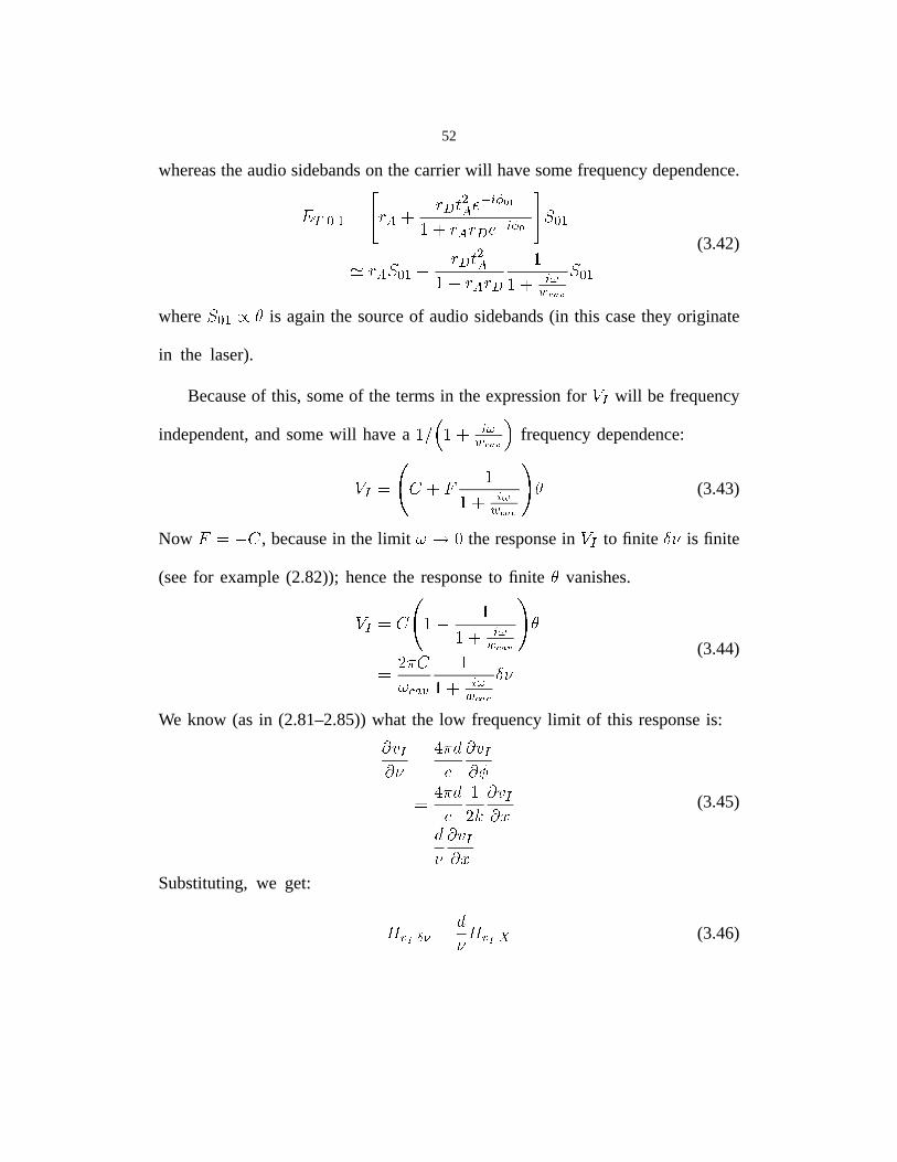
52
whereastheaudiosidebandson thecarrierwill havesomefrequencydependence.
��������� ��� � ����������������� ����� � ��� � �!�
" �#�
�� " �#� � � �� ��$�
�� � �&%'�(*)!+
" �,� (3.42)
where" �#� -
is againthe sourceof audiosidebands(in this casethey originate
in the laser).
Becauseof this, someof the termsin theexpressionfor .0/ will be frequency
independent,andsomewill havea�21 � � � %' (�)!+ frequencydependence:
. / � 34�65 �� � � %' (*)!+
-(3.43)
Now57� 3
, becausein the limit 8 9 the responsein . / to finite :<; is finite
(seefor example(2.82)); hencethe responseto finite-
vanishes.
. / �=3 � �� � � %' (*)!+
-
�?>�@ 38BA�CED
�� � �&%' (�)!+ :<;
(3.44)
We know (as in (2.81–2.85))what the low frequencylimit of this responseis:F�G /F ;
�IHJ@�KL
FMG /FON�IHJ@�K
L�
><PFMG /FMQ
�RK;
FMG /FMQ
(3.45)
Substituting,we get:
S DUT�VXW �RK;
S DYT[Z (3.46)
53
3.2 Response of the Complete Interferometer
At this point we arereadyto computethe frequencyresponsecorresponding
to the derivativeswe found in Chapter2. We will proceedin roughly the same
orderaswe did there,finding first theresponse,asa functionof frequency,in the
gravitationalwave output ��� and in ��� , the isolator quadraturephaseoutput, to
���and � � . Theseresponsesarerelativelysimplebecausefor eachof themeither
theaudiosidebandson thecarrieror theaudiosidebandson theRF sidebandscan
be ignored.Moreover,we will arguethat the transmissionfunction for the audio
sidebandson the RF sidebandsis frequencyindependent;this further simplifies
two of the transfer functions.
Next we will analyzethe responsein thecommon-modeoutputs�� and �� to
� �and � � . The responsesto � � arethe mostcomplexoneswe will encounter.
In theseresponses,all of theaudiosidebandscontributesignificantlyto thesignal.
Throughoutour analysisof frequencyresponse,we will restrictour attention
to frequenciesmuchsmallerthanthe free spectralrangeof an arm cavity:
��������� � (3.47)
(where ������� ����� �� � ). This allows us to makea numberof simplifying
approximations,andmoreovergivesus all of the informationwe needto design
any of the servoloops which will feed back to a force on a mirror, sinceall of
theseloopsareconstrainedto haveunity-gainfrequenciesmuchsmallerthanthe
54
arm cavity free spectralrange,due to internal resonancesin the mirrors. The
loop which feedsback to the laserfrequencycanhavea bandwidthapproaching
or evenexceedingthearm cavity free spectralrange;hereour analysisis of little
help. For this one loop we rely on a numericalmodel (seeChapter4) to verify
that the interferometertransferfunction is sufficiently well behavedto permit us
to implementa stablecontroller.
Differential Signals
We beginour characterizationof the interferometerwith the signal in which
wewouldobservegravitationalwaves.SupposethemirrorsIB andPBareshaking
at frequency � with oppositephase. Eachwill be a sourceof audio sidebands
on the carrierandthesesidebandswill propagateout to the beamsplitter. At the
beamsplitter, they will interferealmostperfectlydestructivelyon the symmetric
side and almostperfectly constructivelyon the antisymmetricside. The reason
that the interferenceis not perfect is that one pair hashad to travel a distance
�farther than the other. For an asymmetryof 57 cm and an audio sideband
wavelengthof ���������� �������� (correspondingto a shakingfrequencyof 10kHz),
a fraction ������ ���� �"!$#&%(' )+*-, ) ��. / of the audio sidebandpower is diverted
from the antisymmetricport to the symmetricport. We will ignore this effect.
Againwe ignoretheeffectof thearmcavitybackmirrorson theRFsidebands.
Theneachtermin 0�1 is proportionalto thetransmissionfunctionfrom thesources
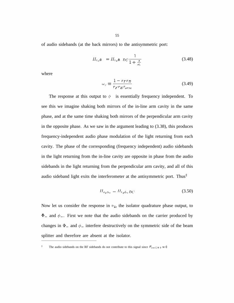
55
of audio sidebands (at the back mirrors) to the antisymmetric port:
����������������� ����� ���� ���� (3.48)
where
��� � �����! � � � �"�#%$�& (3.49)
The response at this output to ')( is essentially frequency independent. To
see this we imagine shaking both mirrors of the in-line arm cavity in the same
phase, and at the same time shaking both mirrors of the perpendicular arm cavity
in the opposite phase. As we saw in the argument leading to (3.38), this produces
frequency-independent audio phase modulation of the light returning from each
cavity. The phase of the corresponding (frequency independent) audio sidebands
in the light returning from the in-line cavity are opposite in phase from the audio
sidebands in the light returning from the perpendicular arm cavity, and all of this
audio sideband light exits the interferometer at the antisymmetric port. Thus‡
� ���+*,� -� ���.*,�/�0�(3.50)
Now let us consider the response in 1,2 , the isolator quadrature phase output, to
3 ( and '4( . First we note that the audio sidebands on the carrier produced by
changes in3 ( and '4( interfere destructively on the symmetric side of the beam
splitter and therefore are absent at the isolator.
‡ The audio sidebands on the RF sidebands do not contribute to this signal since 57698�:<;>=,=@?BA
56
For the response to���
, we consider the compound mirror of Figure 2.8 as
the source of audio sidebands on the RF sidebands. For the cavity in which these
audio sidebands resonate (consisting of the recycling mirror and the compound
back mirror),
������� � ��������������� � ������������� � �!�"� #%$'&)(*�,+.-0/ 21'354 17689;:�:=<?>A@ (3.51)
in our numerical example. This is far outside of the frequency range of interest
and we approximate
�� 4 BCEDGFIH � (3.52)
to get
>KJL!MON >PJLMON�Q�R(3.53)
For the response to S �, as in (2.66), the source is the small audio sidebands
put on the RF sidebands by motion of the arm cavity back mirrors. We repeat
the steps leading up to (3.17), using�UT�V : �XW �?Y�Z�[\�K],^_� for an RF sideband
in an arm cavity, to get
`ba T�T c�dfe�hg C;ikj DGlnm�o
� 4 d ,p e ��g C�i0j DGlrq TUT(3.54)
which is essentially constant in the frequency range of interest. The same thing
is true for the remaining audio sidebands on RF sidebands, and we conclude that
the response is frequency independent:
> JL!stN > JLstN�QfR(3.55)
57
Common-mode Signals
Next we turn to the responseto���
, which correspondsto commonmode
changesof arm cavity length. Whenthe arm cavity backmirrors shakein phase,
the audio sidebandson the carrier interfereconstructivelyat the symmetricside
of the beamsplitter. Becausethe carrier audio sidebandlight coming from the
two arm cavitieshasthe sameamplitudeandphaseandbecauseany of this light
reflectedback towardsthe cavitieswill be treatedin the sameway by the two
arm cavities,we can15, for the purposeof calculatingthe responseto this type
of mirror motion, replacethe beamsplitter and arm cavitieswith a single arm
cavity, as shown in Figure 3.2.
Figure 3.2 Equivalentsystemfor the purposeof deriving common-moderesponse.
R
BF
The mirrors R and F form a compoundmirror§16,17 with (using (2.15))
reflectivity from the right of
�������� � � ���� ��� �� ��� � �
� � ������� ��� (3.56)
§ Implicit in this simplifying substitutionis the assumptionthat the reflectivity of the compoundmirror is frequency
independent.This is in fact a very good approximation.Letting ������� �"!$#$% (with �"!"#&%'�)(+*% in (2.16), (2.21) gives
roughly , -.�+!$#&% as the rateof changeof phaseof the reflectivity with � . This is exceedinglysmall comparedto �"/0!"1 ,
which is the rateof changeof round-tripphasedueto the lengthof the arm cavity.
58
so that
������������ ���������������� ���� ���� � (3.57)
where
!#"�" � $&%('*)+$&,$&%('�)+$�,-&.�/10 (3.58)
Noting that
2 /436587:9 �;2�=< 0>7:91? ) ?A@ (3.59)
2 /4365�7#BC9 �;2�6< 0>7:BC91?4)?A@ (3.60)
we have immediately
�D�4E6���=�� 8�����4E=���F�8� ���� �� � � (3.61)
It is useful to write our expression for !:"�" , in terms of individual mirror parameters,
in a more compact form. We write
$&% � � GH% %� GI%J %J
(3.62)
where % � KL% G % is the loss in mirror F, and
G @ � � K�@ @ (3.63)
$ ) � GI)J )J (3.64)
59
to get
������� � �� � � �� � ��� � � ��� � � � ��� � ��� � ��� � � � ���� � �� � � ��� � �� �
� � �� � � �� ��� � ��(3.65)
and*
������� ��� "!$#&% � � � �� �'� � �� � () � ( (3.66)
Unlike our previousexpressionfor �*��� , theevaluationof this expressiondoesnot
requiresubtractingnearly equalnumbers.
Thetransferfunctionsfrom +-, , changesin which correspondto displacement
of all four arm cavity mirrors towards(or away from) the beamsplitter, are the
most complexof the oneswe will analyze. As we saw in the analysisleading
to (2.74), the low-frequencyresponsein the inphasepick-off signal . � is due to
the fact that whenthe recyclingcavity lengthchanges,the carrierphasechanges
in proportionto /10 andthe sidebandphaseschangein proportionto /32 , so that
a signal is producedaccordingto (2.7). To generalizethis result to the caseof
mirror motion at arbitrary frequencies,we first usethe audiosidebandpicture to
explainthesameresult. At very low frequencies(wherethetwo modelsoverlap),
the resultantphasorformedwhenthecarrier(or oneof theRF sidebands)andits
two audio sidebandsare summedis a phasorslowly rotating back and forth at
* The setof termsin parenthesesrepresentsthe setof “leaks” throughwhich carrier light is able to escapefrom the
system. If the laserwere abruptly shut off, it would take the field about1/10 of a secondto decayto 1/e of its initial
amplitude;in fact this stepresponserepresentsan alternateway of calculatingthe frequencyresponseto certaininputs.
60
the shakingfrequency. The frequency-dependentanalogof the statementabove
involving phaseschangingat differentratesis theremarkthat theaudiosidebands
on the RF sidebandsbeatagainstthe carrier,producinga signal which partially
cancelsthe signalproducedwhenthe audiosidebandson the carrierbeatagainst
the RF sidebands.
Now we seethat as the shakingfrequencyincreases,the contributionto the
signalfrom theaudiosidebandson theRFsidebandswill beconstant(asin (3.52))
whereasthecontributiondueto theaudiosidebandson thecarriermayhavesome
frequencydependenceproportionalto the transmissionfunctions�����
and�������
.
Anticipating that� ������� � ���
we write
���������������� � �������� �"!$# � %�&('*),+.-%�&('�) � - # �# � # � (3.67)
Let us find�����
. We considerthe arm cavities and beam splitter as the
compoundback mirror and sourceof audio sidebandsfor the cavity having the
recycling mirror and pickoff as its compoundfront mirror. The reflectivity of
this backmirror is frequencydependent.Using (2.15)with / ���0����� �2143 ��50687:9we get
;�< � 1=3 �"5>6?7:9$� � ;�@ A�B@ ;�CD ;E@F;�C � D �G��5>687:9H�� ;�< � D 7�I7�J &LK ++ JD 3 K ++ J
(3.68)
61
Now accordingto (3.11) and(3.14) with���������
and* ���� �� � we have
������� ���� �������� �"!#�$�&%(')�*�+-,�� ��.0/ �+�
� �� �1� �2!#�1� �
���4365587���93655#7:7/ ��
(3.69)
wherewe haveused† ��;� ���< �>=0?�@�� 7BA�>C �>=0?�@��>D �� . To find E �F<G� , we repeatthe above,
using � insteadof � . andconcludethat EIH�F<G� � E �� . Substitutinginto (3.67),
we get
JLKNM�O�P %�Q . � JLK�M>O$P"RTS �U�VQ WFXWYX < WGA�5#7:7 WGAWFX < WZA
�5#7�U� �
5#7[7(3.70)
Neglecting WGAW X < W A�5 7 next to WFXW X < W A
�5 7:7 we have
J\K�M>O$P %�Q . � JLK�M>O$P2R+S ����] X�^ ] A] X 5_7:7
�U� �5#7[7
(3.71)
To derive the responsein ` � to�aC
, we use exactly the sameargument,
substitutingaugmentedbouncenumbersbdc� and bdc� for the bouncenumbersb �
and b � , to get:
J K X O$P %�Q . � J K X O$P2R+S�e�gfh� WjiXW iX < W iA
�5_7:7 WeiAW iX < W iA
�5#7
���93B55#7[7J K X O$P_R+S
�e� �] iX ^ ] iA] iX 5#7[7
��� �5#7:7
(3.72)
* More relevanthereis the fact that k;l[m n;o1prq&s tvu;w[x"y[z|{~}�y6���U�_�~�;�~���:�† This can be shown to be equal to our previous expression for �8}[} by simplifying as we did in (3.65).
62
wherethe approximateequivalenceagainis derivedby neglecting����� ���� � �� �� next
to� ��� �� � � �� ���� .
Finally, since we intend to feed back to the recycling mirror, we needto
understandthe responseto recyclingmirror motion*. We define ��������
to be the
set of transferfunctionsfrom recycling mirror displacement( ��������� �"!$#&%(' ) to
the mixer outputs. We can seeimmediatelythat
)�*����� � ��*�,+��(3.73)
by an argumentsimilar to the oneadvancedin Section3.1. Therewe found that
for a Fabry-Perotcavity, theeffect of motionof the front mirror differsonly by a
phasefrom theeffect of backmirror motion. If we shaketherecyclingmirror, the
armcavity front mirrors,andthearmcavitybackmirrorsall at thesamefrequency
andin thesamephase,thenagain,to a goodapproximation† we imposeanequal
audiophasemodulationon eachRF frequency,generatingno signal. This means
thatmotionof therecyclingmirror by itself producesa signalequalandopposite‡
to the signal producedby motion of the other four mirrors.
* Togetherwith the responseto beamsplitter motion of AppendixC, this will completethe analysisof the dynamic
responseof the interferometer.
† This result is exactif the mirror motionsarenot exactly in phase,but insteadthe arm cavity front mirrors leadthe
recycling mirror by the time it takeslight to travel acrosstheir respectiveseparations,and the arm cavity back mirrors
leadthe front mirrors by the time it takeslight to travel the lengthof an arm cavity.
‡ This sign differencedoesnot appearin equation(3.73) becausewe use the oppositedirection of motion for the
recyclingmirror to define - � .

63
In thenextchapterwewill compareplotsof thefrequencyresponsecalculated
accordingto our simplified analysisaboveto plots of the responsecalculatedby
a purely numericalmodel,which makesfewer approximations.
64
Chapter 4 Numerical Models
Two numericalmodelshavebeendevelopedfor the purposeof analyzingthe
optical system.
The first one,the “numericalDC model” calculatesthe samederivativesthat
we found in Chapter2§. Written in Mathematica,it finds symbolic expressions
for all of the relevantfields in the interferometer.It then differentiatesthem as
required to find the symbolic derivativesof the mixer outputswith respectto
the phases.BecauseMathematicadoesnot makethe approximationswe did, the
expressionsfor thesederivativesarequitelong, typically filling severalpages.Into
theseexpressionstheprogramsubstitutesnumericalvaluesfor mirror reflectivities
and phases,to generatea table of derivatives. The sameprogramis of course
alsoableto find valuesfor the fields at the outputs;thesenumbersareuseful for
shot noise calculations.
Thesecondmodel,called“Twiddle,” calculatesthefrequencyresponseof the
interferometer.To understandhow it works, we considerthe simpleFabry-Perot
cavity, fed by a sourceof light of unit magnitude.
The equationsfor this systemmay be written
�������(4.1)
§ A modelwhich calculatedthemixer outputsignalsinsteadof their derivativeswaswritten in 1991by S. Whitcomb.
The modeldiscussedherewasadaptedfrom that earliermodel.
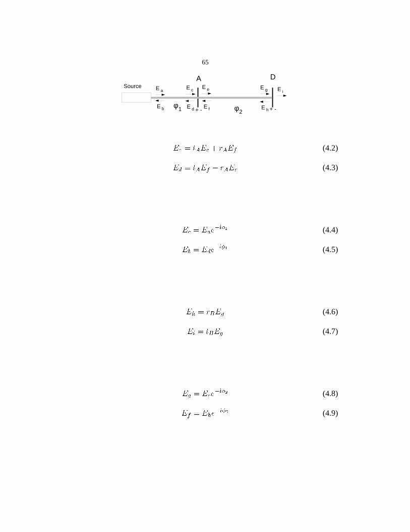
65
A DSource E a
E b
E c E e
E d E f
E g
E h
E i
φ 1 φ 2+ - + -
����������� ��������(4.2)
����������� � �����(4.3)
������������! #"�$(4.4)
��%���� � � �& '"�$(4.5)
��()�*��+,�.-(4.6)
� ��� + ��-(4.7)
��-/�����0���! #"�1(4.8)
� � �2��(3���! '"�1(4.9)
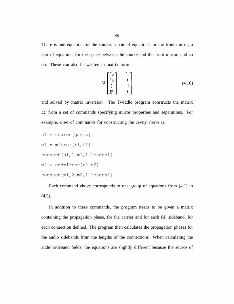
66
Thereis one equationfor the source,a pair of equationsfor the front mirror, a
pair of equationsfor the spacebetweenthe sourceand the front mirror, and so
on. Thesecan also be written in matrix form:
�
������...���
�
�...
(4.10)
and solved by matrix inversion. The Twiddle program constructsthe matrix
�from a set of commandsspecifying mirror propertiesand separations.For
example,a set of commandsfor constructingthe cavity aboveis:
s1 = source[gamma]
m1 = mirror[r1,t1]
connect[s1,1,m1,1,length1]
m2 = endmirror[r2,t2]
connect[m1,2,m2,1,length2]
Eachcommandabovecorrespondsto one group of equationsfrom (4.1) to
(4.9).
In addition to thesecommands,the program needsto be given a matrix
containingthe propagationphase,for the carrier and for eachRF sideband,for
eachconnectiondefined.The programthencalculatesthe propagationphasesfor
the audio sidebandsfrom the lengthsof the connections.When calculatingthe
audio sidebandfields, the equationsare slightly different becausethe sourceof
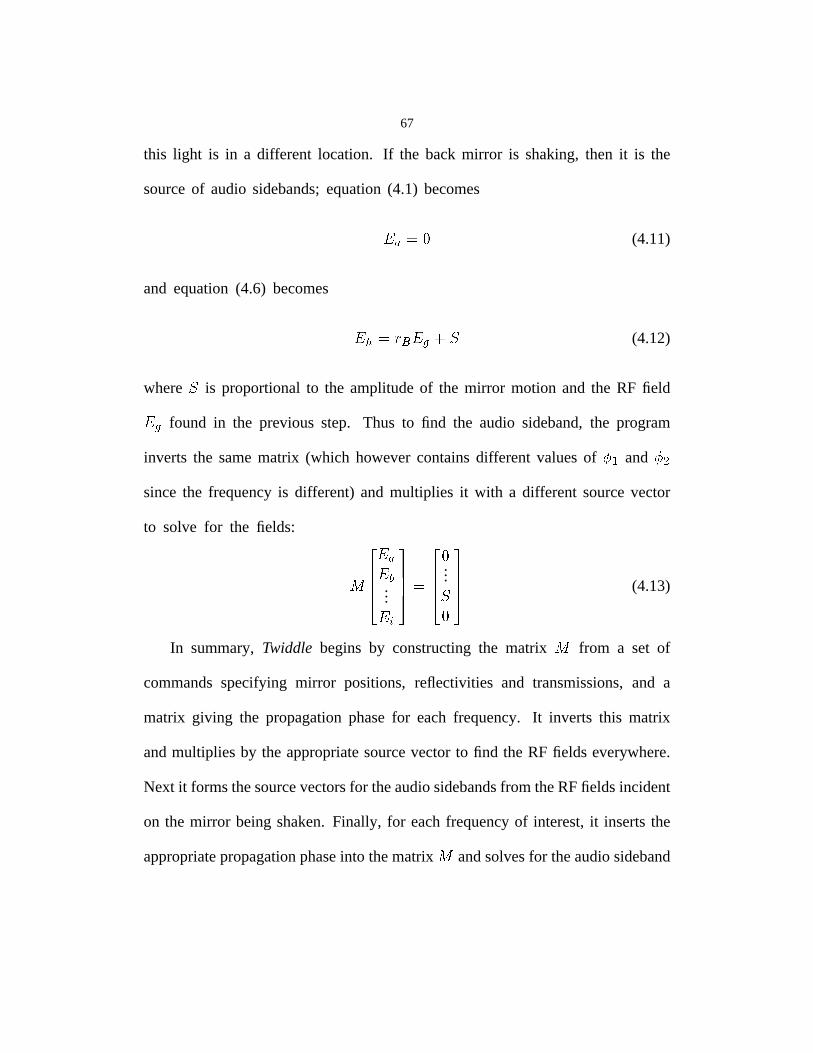
67
this light is in a different location. If the back mirror is shaking,then it is the
sourceof audio sidebands;equation(4.1) becomes
�������(4.11)
and equation(4.6) becomes
����� ���������(4.12)
where�
is proportionalto the amplitudeof the mirror motion and the RF field
���found in the previousstep. Thus to find the audio sideband,the program
inverts the samematrix (which howevercontainsdifferent valuesof ��� and ���sincethe frequencyis different) and multiplies it with a different sourcevector
to solve for the fields:
�������...���
��...��
(4.13)
In summary,Twiddle begins by constructingthe matrix�
from a set of
commandsspecifying mirror positions, reflectivities and transmissions,and a
matrix giving the propagationphasefor eachfrequency. It inverts this matrix
andmultiplies by the appropriatesourcevector to find the RF fields everywhere.
Next it formsthesourcevectorsfor theaudiosidebandsfrom theRFfieldsincident
on the mirror beingshaken.Finally, for eachfrequencyof interest,it insertsthe
appropriatepropagationphaseinto thematrix�
andsolvesfor theaudiosideband
68
fields everywhere.From the valuesof all of thesefields it calculatesthe mixer
output using|| (3.24) or (3.26).
As mentionedearlier,thenumericalmodelshavetheadvantageof beingmore
precisethan the analysesof Chapters2 and 3. Both numericalmodelsinclude
the effectsof loss in the recycling mirror andbeamsplitter andneitherneglects
the RF sidebandfields in the arm cavities. The numerical frequencyresponse
model is not limited to frequenciesmuchsmallerthan the free spectralrangeof
the arm cavitiesand is believedto be accurateup to a significantfraction of the
modulationfrequency.
It is instructive to seehow the calculationscompare. Table 4.1 showsthe
valuesof the derivativescalculatedin Chapter2, evaluatednumerically using
the parametersof Table 1.1, and the derivativescalculatedby the Mathematica
model describedabove. Evidently the amount of accuracysacrificed to the
approximationsmadein Chapter2 is not large.
Theplotsin Figures4.1and4.2showthecomparisonbetweentheapproximate
frequencyresponseanalysisof Chapter3 andthe Twiddle program.Eachplot is
labelledH_nm; the first index indicatesthe output, i.e.,���
through���
, and the
secondindex indicatesthe driven degreeof freedom,i.e., ��� , �� , �� , and �� ,
in that order. We seefrom the plots that the approximateanalysisis goodup to
|| The program containsa generalizedform of theseequationswhich can include the effect of having more RF
frequencies,aswould be appropriatefor larger modulationdepth.
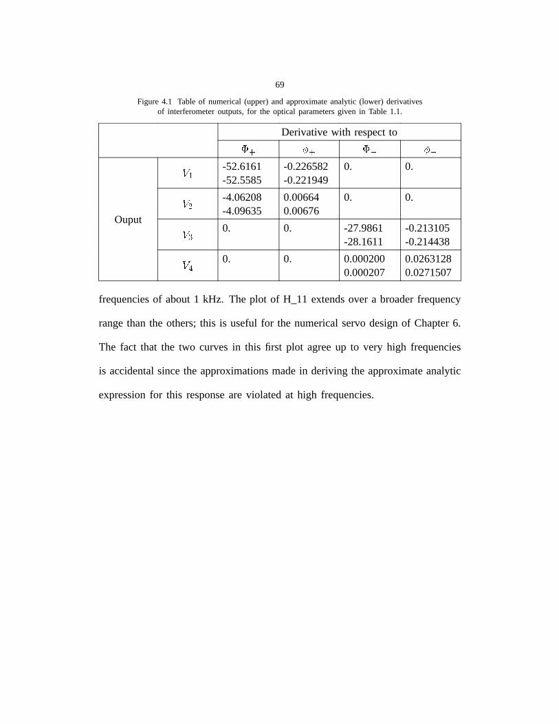
69
Figure 4.1 Tableof numerical(upper)and approximateanalytic (lower) derivativesof interferometeroutputs,for the optical parametersgiven in Table 1.1.
Derivativewith respectto��� ��� ��� ���
� -52.6161-52.5585
-0.226582-0.221949
0. 0.
��� -4.06208-4.09635
0.006640.00676
0. 0.
�� 0. 0. -27.9861-28.1611
-0.213105-0.214438
Ouput
��� 0. 0. 0.0002000.000207
0.02631280.0271507
frequenciesof about1 kHz. The plot of H_11 extendsover a broaderfrequency
rangethanthe others;this is useful for the numericalservodesignof Chapter6.
The fact that the two curvesin this first plot agreeup to very high frequencies
is accidentalsincethe approximationsmadein deriving the approximateanalytic
expressionfor this responseare violated at high frequencies.
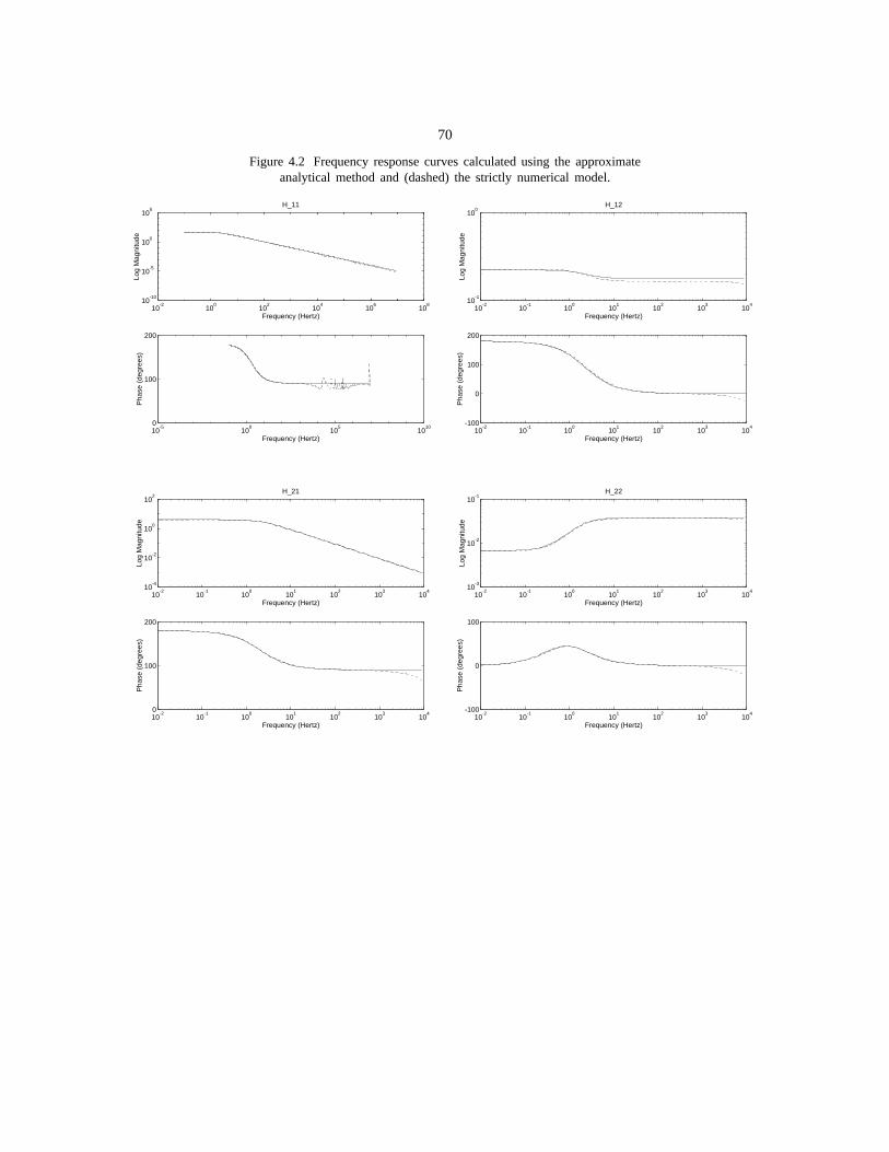
70
Figure 4.2 Frequency response curves calculated using the approximateanalytical method and (dashed) the strictly numerical model.
10-5
100
105
1010
0
100
200
Frequency (Hertz)
Pha
se (
degr
ees)
10-2
100
102
104
106
108
10-10
10-5
100
105
Frequency (Hertz)
Log
Mag
nitu
de
H_11
10-2
10-1
100
101
102
103
104
-100
0
100
200
Frequency (Hertz)
Pha
se (
degr
ees)
10-2
10-1
100
101
102
103
104
10-1
100
Frequency (Hertz)
Log
Mag
nitu
de
H_12
10-2
10-1
100
101
102
103
104
0
100
200
Frequency (Hertz)
Pha
se (
degr
ees)
10-2
10-1
100
101
102
103
104
10-4
10-2
100
102
Frequency (Hertz)
Log
Mag
nitu
de
H_21
10-2
10-1
100
101
102
103
104
-100
0
100
Frequency (Hertz)
Pha
se (
degr
ees)
10-2
10-1
100
101
102
103
104
10-3
10-2
10-1
Frequency (Hertz)
Log
Mag
nitu
de
H_22
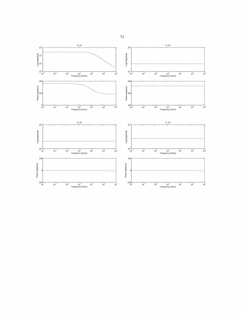
71
10-2
10-1
100
101
102
103
104
0
100
200
Frequency (Hertz)
Pha
se (
degr
ees)
10-2
10-1
100
101
102
103
104
10-1
100
101
102
Frequency (Hertz)
Log
Mag
nitu
de
H_33
10-2
10-1
100
101
102
103
104
100
150
200
Frequency (Hertz)
Pha
se (
degr
ees)
10-2
10-1
100
101
102
103
104
10-1
100
Frequency (Hertz)
Log
Mag
nitu
de
H_34
10-2
10-1
100
101
102
103
104
-100
0
100
Frequency (Hertz)
Pha
se (
degr
ees)
10-2
10-1
100
101
102
103
104
10-4
10-3
Frequency (Hertz)
Log
Mag
nitu
de
H_43
10-2
10-1
100
101
102
103
104
-100
0
100
Frequency (Hertz)
Pha
se (
degr
ees)
10-2
10-1
100
101
102
103
104
10-2
10-1
Frequency (Hertz)
Log
Mag
nitu
de
H_44
72
Chapter 5 Experiments withthe Table-top Prototype
Severaltable-topoptical configurationsof gradually increasingcomplexity
weresetup over the pastseveralyears.This setof experimentsculminatedwith
theconstructionof a completeinterferometerto bedescribedlater in this chapter.
The formal goal of theseexperimentswas to verify a reasonablenumberof the
predictionsof the low-frequencyoptical model#. A secondarymotivation was
simply to demonstratethe generalfeasibility of this extractionscheme.A large
numberof unmodelledeffects could in principle make the operationof sucha
configurationimpractical: extremesensitivity to misalignment,to asymmetryin
losses,to mirror imperfections,or difficulty in acquiring lock being important
examples. Although the successfulconstructionof a small scaleprototypeby
no meansproves that none of theseeffects will be important in a full-sized
interferometer,it nonethelessgives one somecomfort.
The first section of this chaptercontainsa descriptionof the parts from
which all of the experimentswere set up. The following sectionsdescribe
the experimentsin order of increasingcomplexity, from the method used to
characterizethe displacementtransducers,to the characterizationof a simple
# It is difficult to test the frequencyresponsemodel in a table-topexperimentbecausethe lengths(hencedelays)
are shorterand the losseslarger; both of theseeffects lead to optical characteristicfrequencieshard to attain with the
displacementtransducersused.
73
Fabry-Perotcavity, to the characterizationof the three-mirror“coupled cavity”
interferometer,andfinally, to the characterizationof the full interferometer.
5.1 Setup and Hardware
All of the experimentsdescribedin this chapterhave in common certain
aspectsof the setup and certain building blocks from which the optical and
control configurationswereassembled.A (CoherentInnova100) argon-ionlaser
operatingat 514 nm servedas the light source. This laser had beenmodified
by replacing its factory-installedmirrors with mirrors glued to piezo-electric
transducers,sothatthelengthof thelasercavity,andtherebythelaserwavelength
could be adjustedelectrically. Furthermoretwo Pockelscells (Gs̈angerPM 25)
outsideof the lasercavity were usedto effect high-frequencycorrectionsto the
laser wavelength. Thesefeedbackelementswere driven by a high-bandwidth,
low noiseamplifier in a configurationwhich madeit possiblesimply to connect
the demodulatedsignal from an appropriatephotodetectorto the amplifier input
in order to lock the laserfrequencyto a cavity. This setuphadpreviouslybeen
usedwith anotherprototypewithin the LIGO project, and was easily adapted
for the work describedhere. The laser light was phasemodulatedat 12.33
MHz by an additional Pockelscell (Gs̈angerPM 25), which was driven by a
power amplifier (LIGO 5 Watt Amp #9) and impedance-matchingtransformer
(LIGO Step-UpTransformer).Then the laserbeampassedthroughan acousto-
74
optic modulator(Intra-Action AFD 402) usedfor power stabilization,througha
single-modeopticalfiber to improvethebeamquality,andthroughapairof mode-
matchinglensesusedto producea beamwith a convenientwaistsizeandlocation.
Beforeenteringthefiber,aportionof thebeamwasdivertedto anopticalspectrum
analyzerwhich wasusedto checkwhetherthe laserwasoperatingsingle-mode,
andafter the fiber, a portion wasdivertedto a “referencecavity,” a Fabry-Perot
cavity to which the laserfrequencycould be lockedwhena stablefrequencywas
necessary(for exampleduring alignmentof the interferometer). Also after the
fiber, a strayreflectionfrom a mode-matchinglenscaughton a photodetectorwas
usedto stabilizethe power leavingthe fiber, by feedingthe photodetectorsignal
back to the acousto-opticmodulator. A roughly 4 by 10 foot areaof optical
tablewasreservedfor the constructionof variousinterferometers.A transparent
plastic cover with plastic curtainswas installedover this areato protectit from
air currentsand from dust. A small blower equippedwith a filter was installed
for the purposeof purging the enclosedvolumewith dust-freeair. In addition,a
cleanbenchin the room was operatedwheneverdoing so did not interferewith
theexperiments.Unfortunately,it wasnecessaryto shutoff both thecleanbench
and the blower wheneverit wasdesiredto havean interferometerresonatingon
the table.
An RF signal was usedfor phasemodulationand as a signal to drive the
mixers. Figure 5.1 shows the setup used to generateand distribute the RF
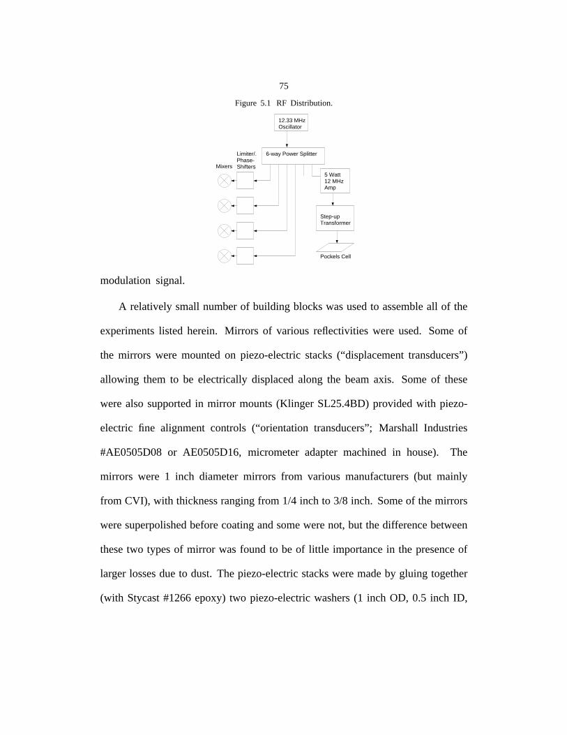
75
Figure 5.1 RF Distribution.
12.33 MHzOscillator
6-way Power SplitterLimiter/.Phase-ShiftersMixers
Step-up Transformer
5 Watt12 MHz Amp
Pockels Cell
modulationsignal.
A relatively small numberof building blockswasusedto assembleall of the
experimentslisted herein. Mirrors of variousreflectivitieswere used. Someof
the mirrors were mountedon piezo-electricstacks(“displacementtransducers”)
allowing them to be electrically displacedalong the beamaxis. Someof these
werealsosupportedin mirror mounts(Klinger SL25.4BD)providedwith piezo-
electric fine alignment controls (“orientation transducers”;Marshall Industries
#AE0505D08or AE0505D16, micrometeradaptermachinedin house). The
mirrors were 1 inch diametermirrors from various manufacturers(but mainly
from CVI), with thicknessrangingfrom 1/4 inch to 3/8 inch. Someof themirrors
weresuperpolishedbeforecoatingandsomewerenot, but thedifferencebetween
thesetwo typesof mirror wasfound to be of little importancein the presenceof
larger lossesdueto dust. The piezo-electricstacksweremadeby gluing together
(with Stycast#1266epoxy) two piezo-electricwashers(1 inch OD, 0.5 inch ID,
76
type 550, from PiezoKinetics) with brasswashersservingasthe electrodes.The
mechanicaldesignof the assemblyof mirror mounts,displacementtransducers,
and orientation transducerswas adopted,with only minor modifications, from
experiments18,19,20performedat the MassachusettsInstituteof Technology.
Two typesof photodiodeswere used: tunedRF photodiodesmadein house
(LIGO #5 and #6), and broadbandPIN photodiodes(ThorlabsDET1–Si); the
bandwidthof the latter type dependson the load impedance.Photodiodeswere
usedin two applications: low-bandwidthapplicationswherethe power at some
optical output was measured(here the Thorlabsdiodeswere usedwith a 5 k
ohmload),andRF applicationsin which fluctuationsin theoutputintensityat the
modulationfrequencyweremeasured(by demodulating).Eitherthelessexpensive
Thorlabs diodes terminatedin 50 ohms or the in-housetuned diodes (which
provided better signal-to-noiseperformance)were usedin the RF applications.
The high-bandwidthphotodiodeswere sometimesfollowed with an amplifier
(LIGO ComlinearE103 CompositeAmplifier, #MEZ 8/17/84, or 1/3 of LIGO
Triple W/B Amp) butalwayswith amixer. Doublebalancedmixers(Mini-Circuits
ZAY–1) were used, followed by low-pass filters to remove the modulation-
frequency componentsfrom the mixer output. The mixers were driven by
limiter/phaseshifters(LIGO #3,9,10and12), deviceswhich containanadjustable
delay line and a limiting and filtering circuit, so that the output is of fixed
amplitude(9 V peak to peak) but the phasedelay is adjustablewith a pair of
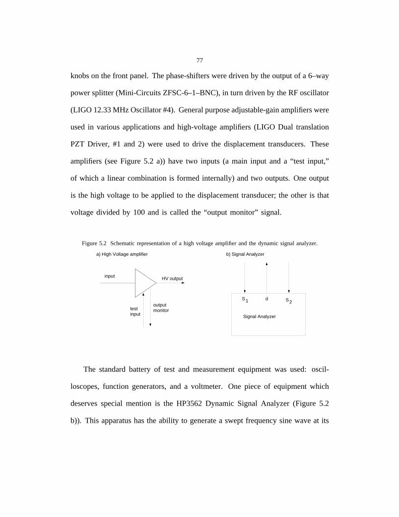
77
knobson thefront panel.Thephase-shiftersweredrivenby theoutputof a 6–way
powersplitter(Mini-Circuits ZFSC-6–1–BNC),in turn drivenby theRF oscillator
(LIGO 12.33MHz Oscillator#4). Generalpurposeadjustable-gainamplifierswere
usedin variousapplicationsand high-voltageamplifiers(LIGO Dual translation
PZT Driver, #1 and 2) were usedto drive the displacementtransducers.These
amplifiers(seeFigure 5.2 a)) havetwo inputs (a main input and a “test input,”
of which a linear combinationis formedinternally) andtwo outputs.Oneoutput
is the high voltageto be appliedto the displacementtransducer;the other is that
voltagedivided by 100 and is called the “output monitor” signal.
Figure5.2 Schematicrepresentationof a high voltageamplifier andthe dynamicsignalanalyzer.
a) High Voltage amplifier
input
test input
outputmonitor
HV output
Signal Analyzer
S1 d S2
b) Signal Analyzer
The standardbattery of test and measurementequipmentwas used: oscil-
loscopes,function generators,and a voltmeter. One pieceof equipmentwhich
deservesspecialmention is the HP3562Dynamic Signal Analyzer (Figure 5.2
b)). This apparatushasthe ability to generatea sweptfrequencysinewaveat its
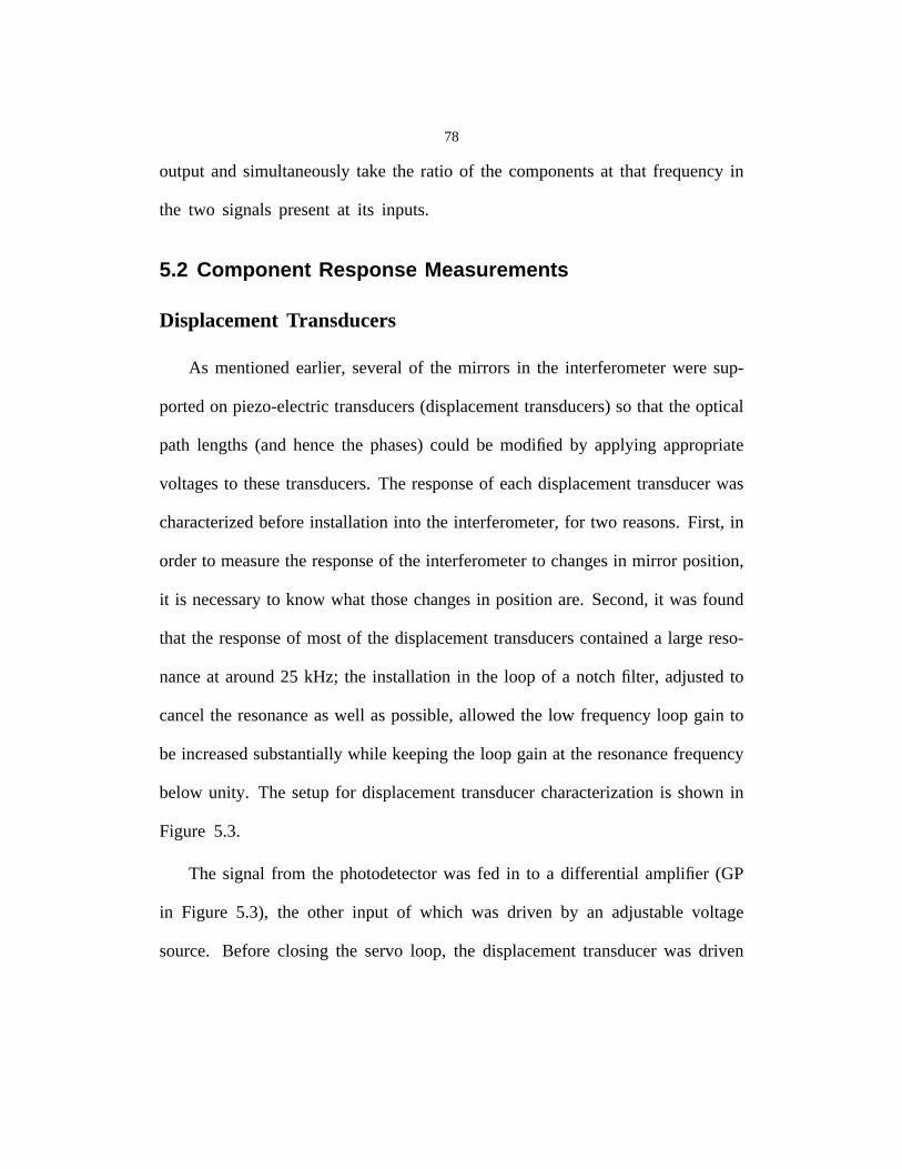
78
output and simultaneouslytake the ratio of the componentsat that frequencyin
the two signalspresentat its inputs.
5.2 Component Response Measurements
Displacement Transducers
As mentionedearlier, severalof the mirrors in the interferometerwere sup-
portedon piezo-electrictransducers(displacementtransducers)so that theoptical
path lengths(and hencethe phases)could be modified by applying appropriate
voltagesto thesetransducers.The responseof eachdisplacementtransducerwas
characterizedbeforeinstallationinto the interferometer,for two reasons.First, in
orderto measurethe responseof the interferometerto changesin mirror position,
it is necessaryto know what thosechangesin positionare. Second,it wasfound
that the responseof mostof the displacementtransducerscontaineda large reso-
nanceat around25 kHz; the installationin the loop of a notchfilter, adjustedto
cancelthe resonanceaswell aspossible,allowedthe low frequencyloop gain to
be increasedsubstantiallywhile keepingthe loop gainat the resonancefrequency
below unity. The setupfor displacementtransducercharacterizationis shownin
Figure 5.3.
The signal from the photodetectorwas fed in to a differential amplifier (GP
in Figure 5.3), the other input of which was driven by an adjustablevoltage
source. Before closing the servo loop, the displacementtransducerwas driven
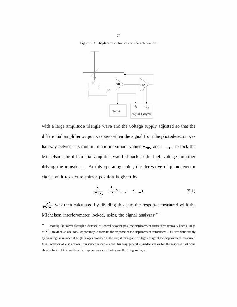
79
Figure 5.3 Displacementtransducercharacterization.
S1 d S2
ScopeSignal Analyzer
GP HV
with a large amplitudetrianglewaveandthe voltagesupplyadjustedso that the
differentialamplifieroutputwaszerowhenthesignalfrom thephotodetectorwas
halfway betweenits minimum andmaximumvalues ������� and ������ . To lock the
Michelson,the differential amplifier was fed back to the high voltageamplifier
driving the transducer.At this operatingpoint, the derivative of photodetector
signal with respectto mirror position is given by
���� ������
���� � ������ ������� ��� (5.1)
���! #"%$�'&)(+*-,/.10 was then calculatedby dividing this into the responsemeasuredwith the
Michelsoninterferometerlocked,using the signal analyzer.**
** Moving the mirror througha distanceof severalwavelengths(the displacementtransducerstypically havea range
of 2354 ) providedanadditionalopportunityto measuretheresponseof thedisplacementtransducers.This wasdonesimply
by countingthenumberof bright fringesproducedat theoutputfor a givenvoltagechangeat thedisplacementtransducer.
Measurementsof displacementtransducerresponsedone this way generallyyielded valuesfor the responsethat were
abouta factor 1.7 larger thanthe responsemeasuredusingsmall driving voltages.
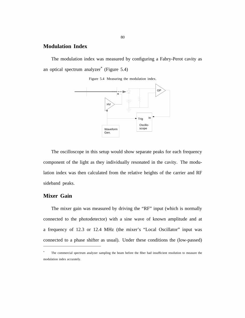
80
Modulation Index
The modulationindex was measuredby configuringa Fabry-Perotcavity as
an optical spectrumanalyzer* (Figure 5.4)
Figure 5.4 Measuringthe modulationindex.
Oscillo-scope
GP
HV
In
WaveformGen.
Trig
The oscilloscopein this setupwould showseparatepeaksfor eachfrequency
componentof the light as they individually resonatedin the cavity. The modu-
lation index was then calculatedfrom the relative heightsof the carrier and RF
sidebandpeaks.
Mixer Gain
The mixer gain wasmeasuredby driving the “RF” input (which is normally
connectedto the photodetector)with a sine wave of known amplitudeand at
a frequencyof 12.3 or 12.4 MHz (the mixer’s “Local Oscillator” input was
connectedto a phaseshifter as usual). Under theseconditionsthe (low-passed)
* The commercialspectrumanalyzersamplingthe beambeforethe fiber had insufficient resolutionto measurethe
modulationindex accurately.
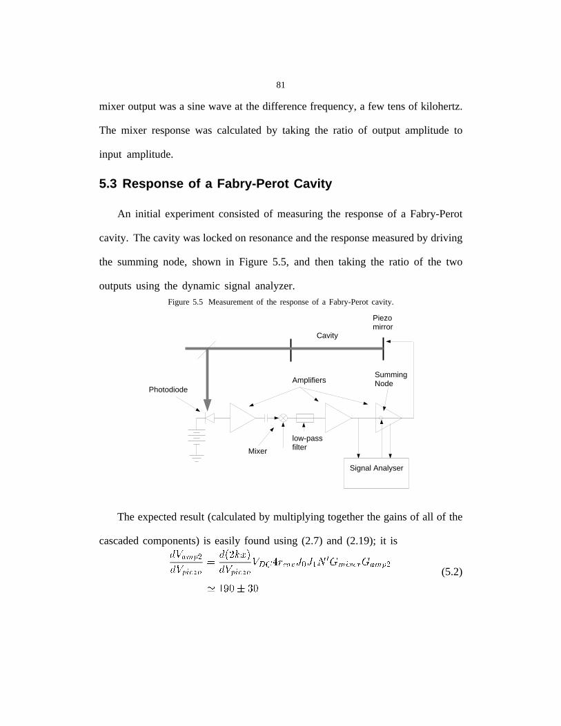
81
mixer output was a sine wave at the difference frequency, a few tens of kilohertz.
The mixer response was calculated by taking the ratio of output amplitude to
input amplitude.
5.3 Response of a Fabry-Perot Cavity
An initial experiment consisted of measuring the response of a Fabry-Perot
cavity. The cavity was locked on resonance and the response measured by driving
the summing node, shown in Figure 5.5, and then taking the ratio of the two
outputs using the dynamic signal analyzer.Figure 5.5 Measurement of the response of a Fabry-Perot cavity.
Cavity
Piezomirror
Signal Analyser
AmplifiersPhotodiode
Mixer
low-passfilter
SummingNode
The expected result (calculated by multiplying together the gains of all of the
cascaded components) is easily found using (2.7) and (2.19); it is�������������� ���������
����������������������� �! #"%$�&(')�+*-,�.�,�/�021�34�5�76��8934�+���(
:;-< =�<(5.2)
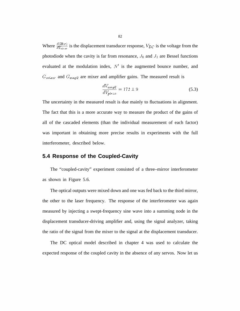
82
Where������������ ��������� is thedisplacementtransducerresponse,����� is thevoltagefrom the
photodiodewhenthecavity is far from resonance,��� and ��� areBesselfunctions
evaluatedat the modulation index, "! is the augmentedbouncenumber, and
#%$'& ��(�) and#%*+$-, � aremixer andamplifier gains. The measuredresult is
. � *+$/, �. � ,& (103254687�9 :
(5.3)
Theuncertaintyin themeasuredresult is duemainly to fluctuationsin alignment.
The fact that this is a moreaccurateway to measurethe productof the gainsof
all of the cascadedelements(than the individual measurementof eachfactor)
was important in obtaining more preciseresults in experimentswith the full
interferometer,describedbelow.
5.4 Response of the Coupled-Cavity
The “coupled-cavity” experimentconsistedof a three–mirrorinterferometer
as shown in Figure 5.6.
Theopticaloutputsweremixeddownandonewasfedbackto thethird mirror,
the other to the laser frequency. The responseof the interferometerwas again
measuredby injecting a swept-frequencysinewave into a summingnodein the
displacementtransducer-drivingamplifier and, using the signal analyzer,taking
theratio of thesignalfrom themixer to thesignalat thedisplacementtransducer.
The DC optical model describedin chapter4 was used to calculate the
expectedresponseof thecoupledcavity in theabsenceof anyservos.Now let us
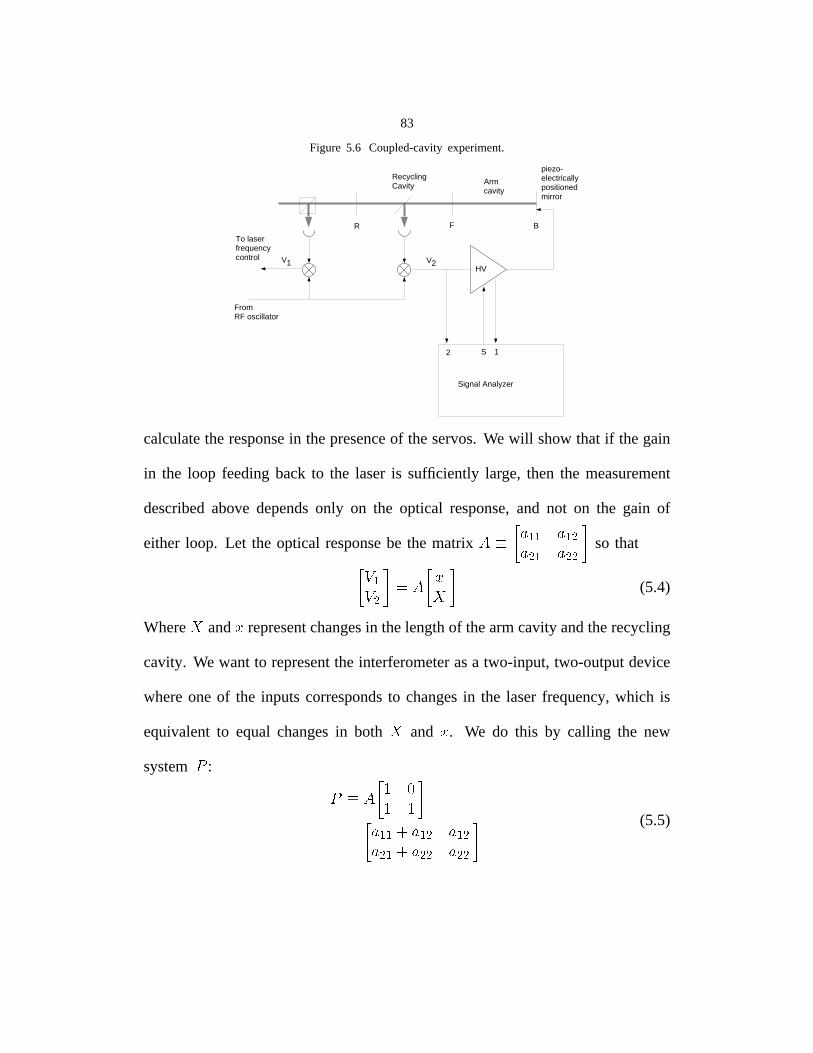
83
Figure 5.6 Coupled-cavityexperiment.
FromRF oscillator
To laser frequencycontrol
piezo-electrically positioned mirror
Signal Analyzer
S 12
Recycling Cavity Arm
cavity
V1 V2HV
R F B
calculatetheresponsein thepresenceof theservos.We will showthat if thegain
in the loop feedingback to the laser is sufficiently large, then the measurement
describedabovedependsonly on the optical response,and not on the gain of
either loop. Let the optical responsebe the matrix� ����� �����
���� ����� so that
� �� � � (5.4)
Where
and � representchangesin thelengthof thearmcavityandtherecycling
cavity. We want to representthe interferometerasa two-input, two-outputdevice
whereoneof the inputs correspondsto changesin the laserfrequency,which is
equivalentto equal changesin both
and � . We do this by calling the new
system � :
�� � �
� �
� ������������� ������������������ �����
(5.5)
84
so that
������ ���
����� ��� (5.6)
where � is the cavity length and � the optical wavelength.
The two feedbackamplifierswe group into a “controller”
� � � � �� � � (5.7)
Figure 5.7 Block diagramof the control systemfor the coupled-cavityexperiment.
d fe
s1
s2
P
C
Then the closed-loopresponsecan be calculatedwith simple matrix manip-
ulations†: �� ������� � ��
����� � �! #"� �� (5.8)
† Historically, in control theory, the points in the loop where signals are summedin have often been taken as
differencing,ratherthansummingnodes.This conventionbecomesawkwardif nodesexist at severalpoints in a loop or
if no nodesexist at all (the latter caseis of interestwhenanalyzingstability). We will usethe conventionthatno changes
of sign occur exceptwherethey are explicitly included. Becauseof this, someof the expressionswe derive may differ
by a sign from expressionsfound in sometextbooks.
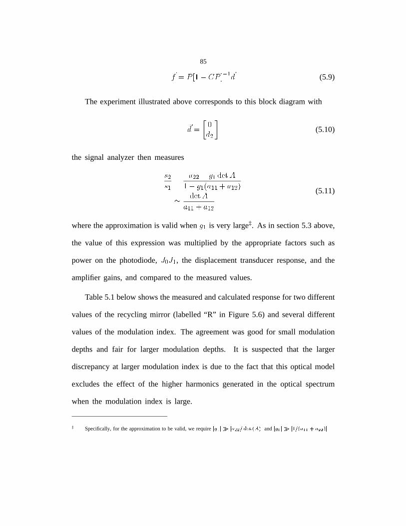
85��������� �� ����� ��(5.9)
The experimentillustratedabovecorrespondsto this block diagramwith
���� ���� (5.10)
the signal analyzerthen measures
� �� �
� � ��� � ����� �"!� � �$# � �%�'& � � �)(�*�+�"!
� ���,& � � �(5.11)
wheretheapproximationis valid when� � is very large‡. As in section5.3 above,
the value of this expressionwas multiplied by the appropriatefactors such as
power on the photodiode, -/.0- � , the displacementtransducerresponse,and the
amplifier gains,and comparedto the measuredvalues.
Table5.1belowshowsthemeasuredandcalculatedresponsefor two different
valuesof the recycling mirror (labelled“R” in Figure 5.6) and severaldifferent
valuesof the modulationindex. The agreementwas good for small modulation
depthsand fair for larger modulation depths. It is suspectedthat the larger
discrepancyat larger modulationindex is due to the fact that this optical model
excludesthe effect of the higher harmonicsgeneratedin the optical spectrum
when the modulationindex is large.
‡ Specifically,for the approximationto be valid, we require 1 2�3416571 8:9;96<>=@?BA>CEDGFB1 and 1 2:361:5H1 IJ<4CK8@3;3MLN8:9;94FO1
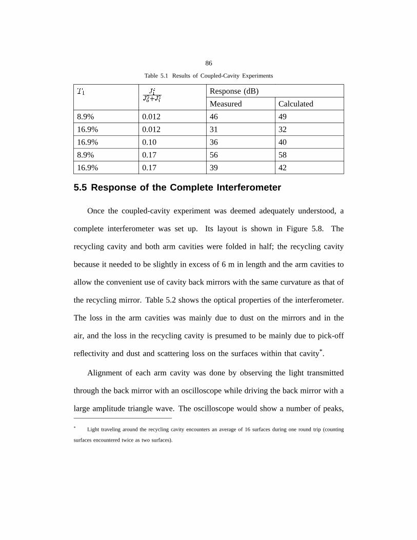
86
Table 5.1 Resultsof Coupled-CavityExperiments
��� ����� ��� � ��Response(dB)
Measured Calculated
8.9% 0.012 46 49
16.9% 0.012 31 32
16.9% 0.10 36 40
8.9% 0.17 56 58
16.9% 0.17 39 42
5.5 Response of the Complete Interferometer
Once the coupled-cavityexperimentwas deemedadequatelyunderstood,a
completeinterferometerwas set up. Its layout is shown in Figure 5.8. The
recycling cavity and both arm cavitieswere folded in half; the recycling cavity
becauseit neededto beslightly in excessof 6 m in lengthandthearmcavitiesto
allow theconvenientuseof cavity backmirrorswith thesamecurvatureasthatof
the recyclingmirror. Table5.2 showstheopticalpropertiesof the interferometer.
The loss in the arm cavitieswas mainly due to dust on the mirrors and in the
air, andthe loss in the recyclingcavity is presumedto be mainly dueto pick-off
reflectivity anddustandscatteringlosson the surfaceswithin that cavity*.
Alignment of eacharm cavity was doneby observingthe light transmitted
throughthebackmirror with anoscilloscopewhile driving thebackmirror with a
large amplitudetrianglewave. The oscilloscopewould showa numberof peaks,
* Light traveling aroundthe recycling cavity encountersan averageof 16 surfacesduring one round trip (counting
surfacesencounteredtwice astwo surfaces).

87
Table 5.2 Fixed Mass InterferometerOptical Properties
Fabry-PerotArmCavities
Front MirrorTransmission
9 %
Back MirrorTransmission
13 ppm
Losses 0.2 %
FringeVisibility 9 %
Cavity Gain 40
RecyclingCavity RecyclingMirrorTransmission
18 %
Cavity Losses(includingPickoff beams)
16 %
FringeVisibilty 88 %
RecyclingFactor 4
Beamsplitter Contrast 99 %
onefor eachresonanttransversemode,andonefor eachfrequencyof light incident
on the cavity. The heightof the peakcorrespondingto the carrier resonatingin
the(degenerate)01 and10 transversemodeswasthenminimizedby adjustingthe
orientationtransducervoltages.Therecyclingmirror wasalignedby driving both
it and the secondarm steeringmirror (SAS in Figure 5.8) with triangle waves
(at different frequencies)andagainminimizing the peakcorrespondingto the 01
and 10 transversemodes.
The feedbackconfigurationwhich was usedis shown in Figure 5.9†. This
† Althoughthefigureshowsloop 4 driving thebeamsplitter,this drive wasactuallyappliedto thesecondarmsteering
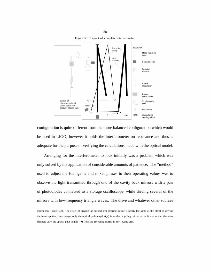
88
Figure 5.8 Layout of completeinterferometer.
Faraday Isolator
Mode-matchinglens
LEGEND
Photodetector
Phase modulation
Power stabilization
Single-mode fiber
Source of phase-modulated, power stabilized, spatially filtered light
Recyclingcavity
Arm cavities
Pickoff
δ
Asymmetryδ
Second arm steering mirror
SASSAS
configurationis quitedifferentfrom themorebalancedconfigurationwhich would
be usedin LIGO; howeverit holds the interferometeron resonanceand thus is
adequatefor thepurposeof verifying thecalculationsmadewith theopticalmodel.
Arranging for the interferometerto lock initially was a problemwhich was
only solvedby theapplicationof considerableamountsof patience.The“method”
usedto adjust the four gainsand mixer phasesto their operatingvalueswas to
observethe light transmittedthroughone of the cavity back mirrors with a pair
of photodiodesconnectedto a storageoscilloscope,while driving severalof the
mirrorswith low-frequencytrianglewaves.Thedrive andwhateverothersources
mirror (seeFigure5.8). The effect of driving the secondarm steeringmirror is nearly the sameas the effect of driving
the beamsplitter; onechangesonly the optical path length (���
) from the recyclingmirror to the first arm, and the other
changesonly the optical path length(���
) from the recyclingmirror to the secondarm.
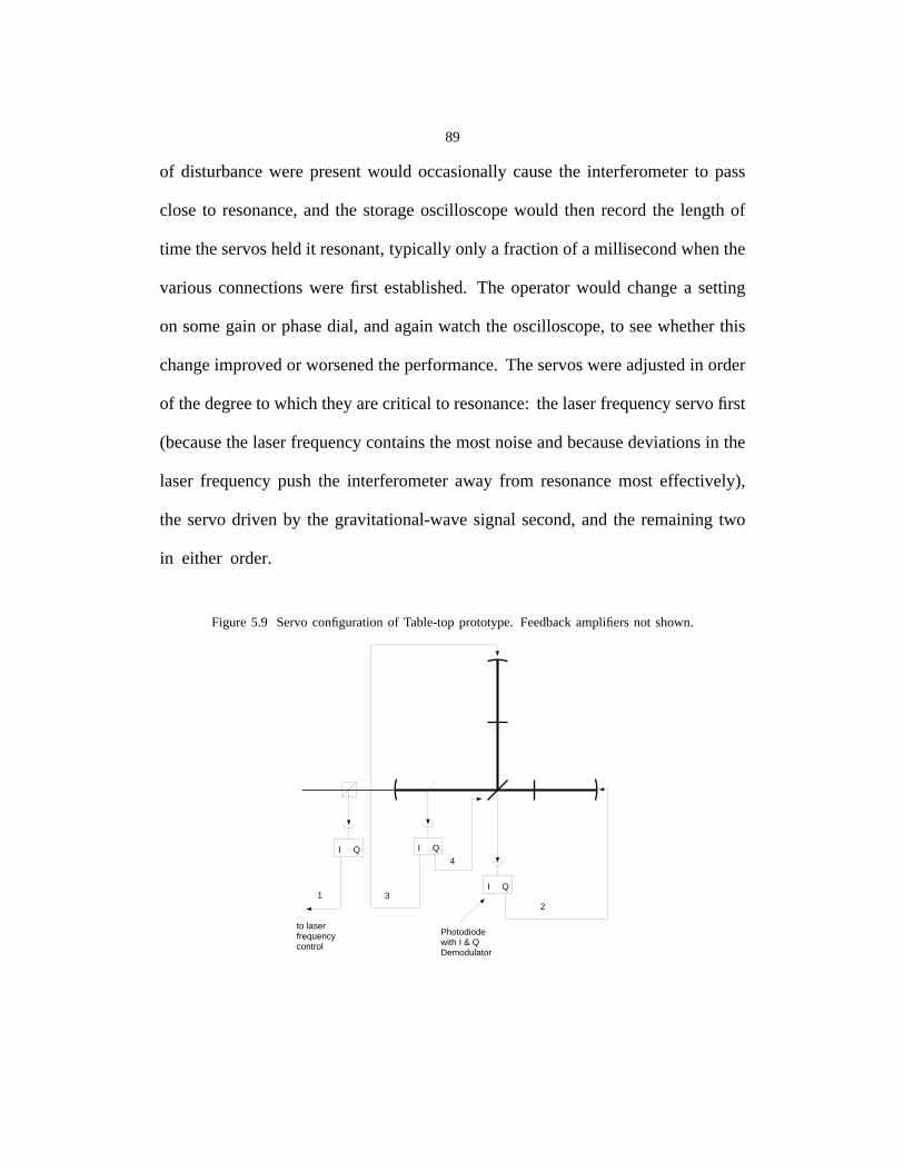
89
of disturbancewere presentwould occasionallycausethe interferometerto pass
closeto resonance,and the storageoscilloscopewould thenrecordthe lengthof
time theservosheldit resonant,typically only a fractionof amillisecondwhenthe
variousconnectionswere first established.The operatorwould changea setting
on somegainor phasedial, andagainwatchtheoscilloscope,to seewhetherthis
changeimprovedor worsenedtheperformance.Theservoswereadjustedin order
of thedegreeto which theyarecritical to resonance:thelaserfrequencyservofirst
(becausethelaserfrequencycontainsthemostnoiseandbecausedeviationsin the
laser frequencypushthe interferometeraway from resonancemost effectively),
the servodriven by the gravitational-wavesignalsecond,and the remainingtwo
in either order.
Figure5.9 Servoconfigurationof Table-topprototype. Feedbackamplifiersnot shown.
I Q
I Q
I Q
Photodiodewith I & Q Demodulator
to laser frequency control
12
3
4
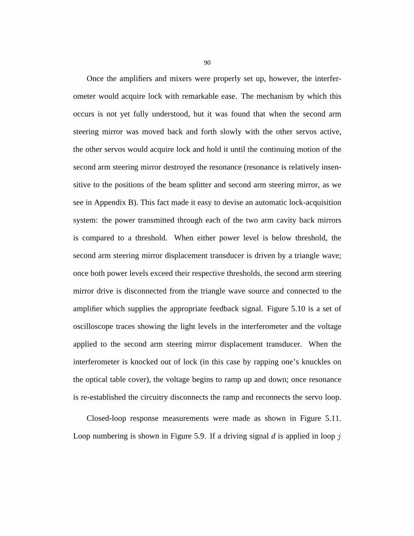
90
Oncethe amplifiersand mixers were properly set up, however,the interfer-
ometerwould acquirelock with remarkableease.The mechanismby which this
occursis not yet fully understood,but it was found that when the secondarm
steeringmirror was movedback and forth slowly with the other servosactive,
theotherservoswould acquirelock andhold it until thecontinuingmotionof the
secondarmsteeringmirror destroyedtheresonance(resonanceis relatively insen-
sitive to the positionsof the beamsplitter andsecondarm steeringmirror, aswe
seein AppendixB). This fact madeit easyto deviseanautomaticlock-acquisition
system: the power transmittedthrougheachof the two arm cavity backmirrors
is comparedto a threshold. When either power level is below threshold,the
secondarm steeringmirror displacementtransduceris driven by a trianglewave;
oncebothpowerlevelsexceedtheir respectivethresholds,thesecondarmsteering
mirror drive is disconnectedfrom the trianglewavesourceandconnectedto the
amplifier which suppliesthe appropriatefeedbacksignal. Figure5.10 is a setof
oscilloscopetracesshowingthe light levels in the interferometerandthe voltage
applied to the secondarm steeringmirror displacementtransducer. When the
interferometeris knockedout of lock (in this caseby rappingone’sknuckleson
theoptical tablecover),thevoltagebeginsto rampup anddown; onceresonance
is re-establishedthecircuitry disconnectstherampandreconnectstheservoloop.
Closed-loopresponsemeasurementswere made as shown in Figure 5.11.
Loop numberingis shownin Figure5.9. If a driving signald is appliedin loop�
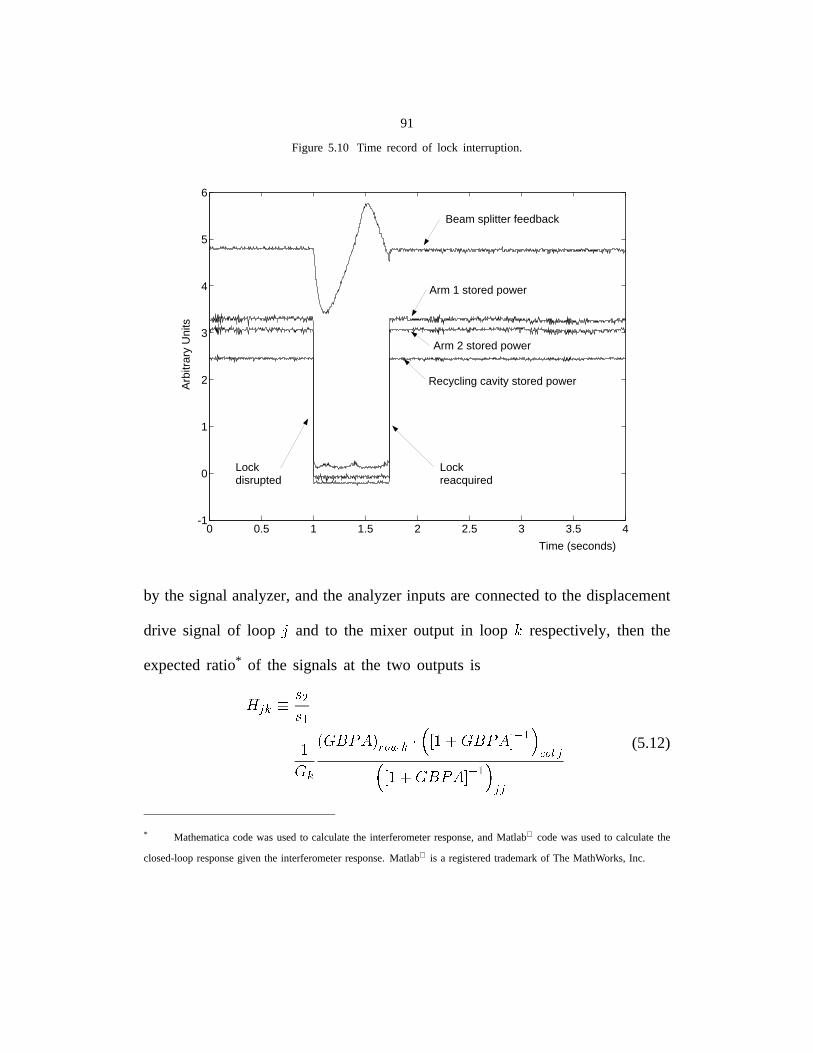
91
Figure 5.10 Time record of lock interruption.
0 0.5 1 1.5 2 2.5 3 3.5 4-1
0
1
2
3
4
5
6
Beam splitter feedback
Arm 1 stored power
Arm 2 stored power
Recycling cavity stored power
Lock reacquired
Lockdisrupted
Time (seconds)
Arb
itrar
y U
nits
by the signal analyzer, and the analyzer inputs are connected to the displacement
drive signal of loop�
and to the mixer output in loop � respectively, then the
expected ratio* of the signals at the two outputs is
����� ����
� � �� ��������������� � � �� �������! #" $ �&% �
� �� �������' " �&�(5.12)
* Mathematica code was used to calculate the interferometer response, and Matlab code was used to calculate the
closed-loop response given the interferometer response. Matlab is a registered trademark of The MathWorks, Inc.
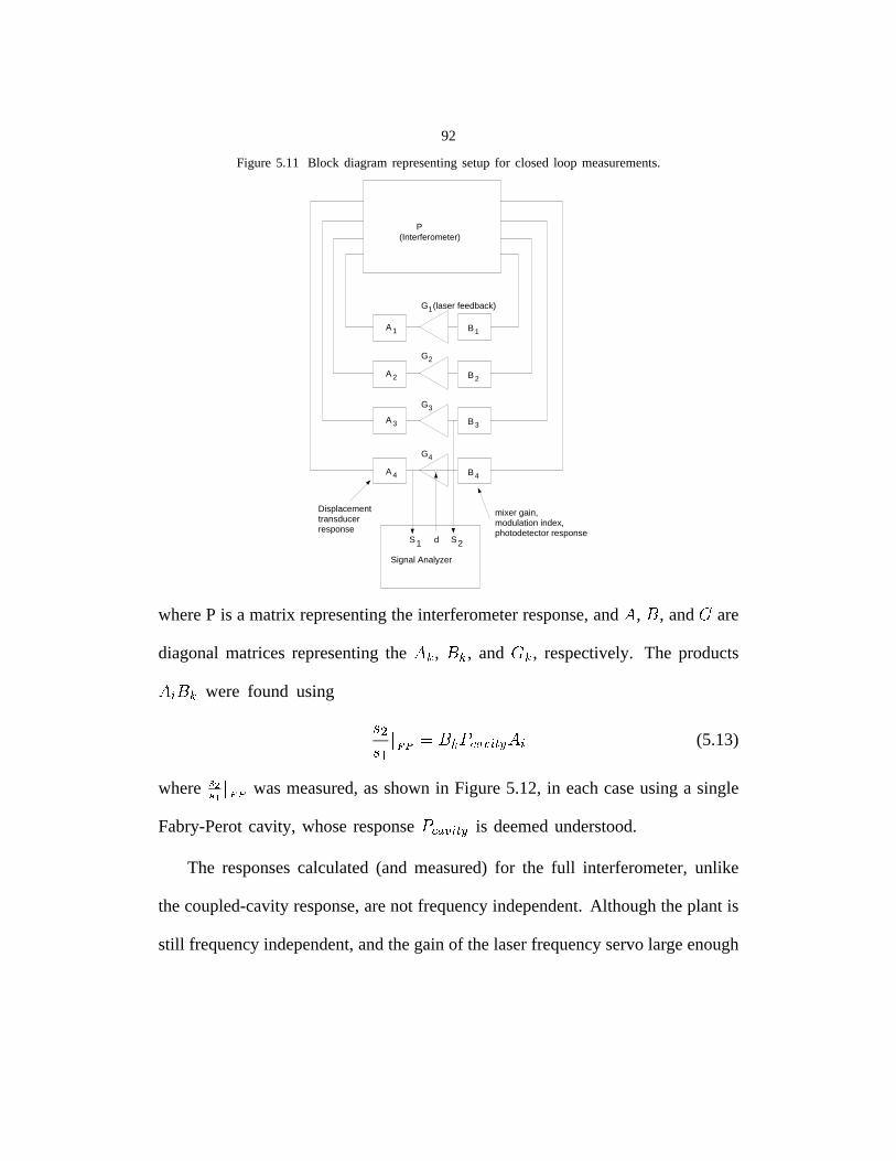
92
Figure 5.11 Block diagram representing setup for closed loop measurements.
A 2
A 3
G (laser feedback)1
G2
G3
G4
B 2
B 3
P(Interferometer)
A 4 B 4
A 1 B 1
Displacementtransducerresponse
mixer gain,modulation index,photodetector response
Signal Analyzer
dS1 S2
where P is a matrix representing the interferometer response, and�
, � , and � are
diagonal matrices representing the���
, � �, and � �
, respectively. The products
��� � �were found using
���� �� �� � ��������� ���������
(5.13)
where ����! �� was measured, as shown in Figure 5.12, in each case using a single
Fabry-Perot cavity, whose response�����"� �#���
is deemed understood.
The responses calculated (and measured) for the full interferometer, unlike
the coupled-cavity response, are not frequency independent. Although the plant is
still frequency independent, and the gain of the laser frequency servo large enough
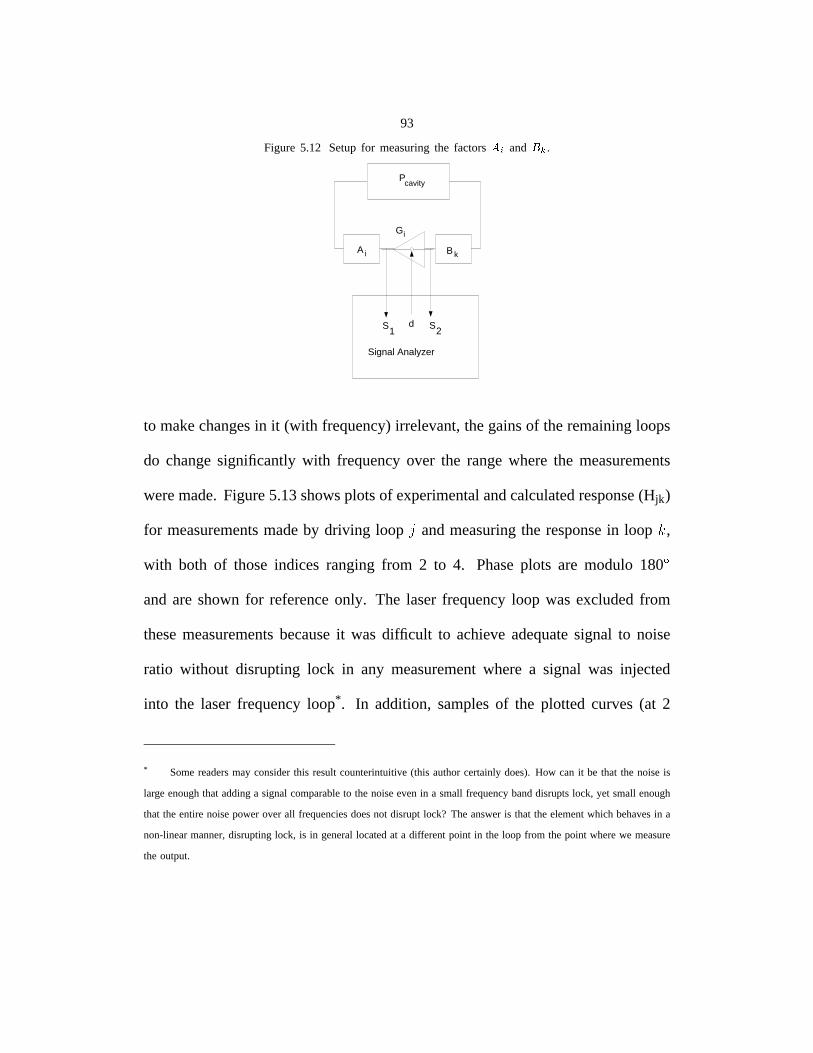
93
Figure 5.12 Setupfor measuringthe factors���
and ��� .
A i
Gi
B k
Pcavity
Signal Analyzer
dS1S2
to makechangesin it (with frequency)irrelevant,thegainsof theremainingloops
do changesignificantly with frequencyover the rangewherethe measurements
weremade.Figure5.13showsplotsof experimentalandcalculatedresponse(Hjk)
for measurementsmadeby driving loop�
andmeasuringthe responsein loop � ,
with both of thoseindices ranging from 2 to 4. Phaseplots are modulo 180�
and are shownfor referenceonly. The laserfrequencyloop was excludedfrom
thesemeasurementsbecauseit was difficult to achieveadequatesignal to noise
ratio without disrupting lock in any measurementwhere a signal was injected
into the laser frequencyloop*. In addition, samplesof the plotted curves(at 2
* Somereadersmay considerthis resultcounterintuitive(this authorcertainlydoes).How can it be that the noiseis
large enoughthat addinga signalcomparableto the noiseevenin a small frequencybanddisruptslock, yet small enough
that the entirenoisepowerover all frequenciesdoesnot disrupt lock? The answeris that the elementwhich behavesin a
non-linearmanner,disruptinglock, is in generallocatedat a differentpoint in the loop from the point wherewe measure
the output.
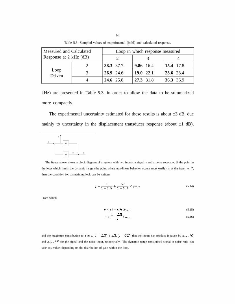
94
Table 5.3 Sampledvaluesof experimental(bold) and calculatedresponse.
MeasuredandCalculatedResponseat 2 kHz (dB)
Loop in which responsemeasured
2 3 4
2 38.3 37.7 9.86 16.4 15.4 17.8
3 26.9 24.6 19.0 22.1 23.6 23.4Loop
Driven4 24.6 25.8 27.3 31.8 36.3 36.9
kHz) are presentedin Table 5.3, in order to allow the data to be summarized
more compactly.
The experimentaluncertaintyestimatedfor theseresultsis about±3 dB, due
mainly to uncertaintyin the displacementtransducerresponse(about ±1 dB),
G
H
s
x
y n
The figure aboveshowsa block diagramof a systemwith two inputs,a signal � anda noisesource � . If the point in
the loop which limits the dynamicrange(the point wherenon-linearbehavioroccursmost easily) is at the input to�
,
thenthe conditionfor maintaininglock canbe written
��� ���� ��� �
� �� ��� ������� (5.14)
From which
� ��� � � ��� � ����� (5.15)
� ���� � ������� (5.16)
andthe maximumcontributionto � ����� � � �� ��� � � � � � � � � � that the inputscanproduceis given by �������!� and ���"���!� � for the signal and the noiseinput, respectively.The dynamicrangeconstrainedsignal-to-noiseratio can
takeany value,dependingon the distributionof gain within the loop.
95
uncertaintyin the lossesin the arm cavities* (about ±1.5 dB), and fluctuations
in alignment(about ±2 dB). All of the plots of experimentalversuscalculated
responseshow reasonableagreementwithin this uncertaintyexceptfor the case
of�����
, wherethe discrepancyis perhapstwice the experimentaluncertainty. It
is not known whetherthis discrepancyis dueto a randomlargefluctuationin the
cumulativeerror or to an unmodeledsystematiceffect.
* The fractionaluncertaintyin the arm cavity roundtrip losswasperhaps+/-50%(dueto fluctuatingdustlevels),but
the correspondingfractionaluncertaintyin the recyclingcavity round trip lossonly about+/-15%, sincearm cavity loss
wasnot the dominantloss in the optical system.
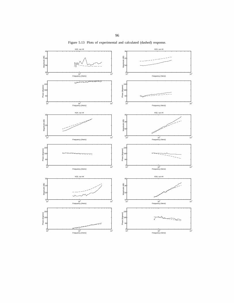
96
Figure 5.13 Plots of experimental and calculated (dashed) response.
102
103
104
0
50
100
150
Frequency (Hertz)
Pha
se (
degr
ees)
102
103
104
36
38
40
42
Frequency (Hertz)
Mag
nitu
de (
dB)
H22, run #4
103
104
0
50
100
150
Frequency (Hertz)
Pha
se (
degr
ees)
103
104
0
10
20
30
Frequency (Hertz)
Mag
nitu
de (
dB)
H23, run #4
103
104
0
50
100
150
Frequency (Hertz)
Pha
se (
degr
ees)
103
104
10
20
30
Frequency (Hertz)
Mag
nitu
de (
dB)
H24, run #4
102
103
104
0
50
100
150
Frequency (Hertz)
Pha
se (
degr
ees)
102
103
104
10
20
30
40
Frequency (Hertz)
Mag
nitu
de (
dB)
H32, run #4
102
103
104
0
50
100
150
Frequency (Hertz)
Pha
se (
degr
ees)
102
103
104
15
20
25
30
Frequency (Hertz)
Mag
nitu
de (
dB)
H33, run #4
102
103
104
0
50
100
150
Frequency (Hertz)
Pha
se (
degr
ees)
102
103
104
10
20
30
40
Frequency (Hertz)
Mag
nitu
de (
dB)
H34, run #4
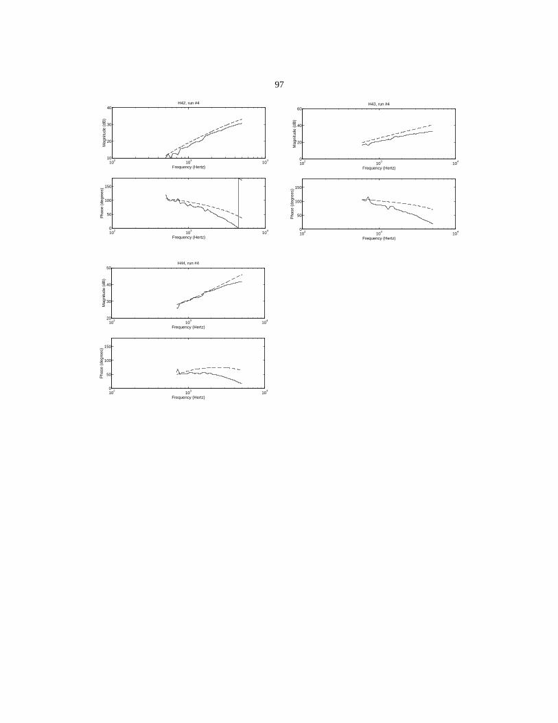
97
102
103
104
0
50
100
150
Frequency (Hertz)
Pha
se (
degr
ees)
102
103
104
10
20
30
40
Frequency (Hertz)
Mag
nitu
de (
dB)
H42, run #4
102
103
104
0
50
100
150
Frequency (Hertz)
Pha
se (
degr
ees)
102
103
104
0
20
40
60
Frequency (Hertz)
Mag
nitu
de (
dB)
H43, run #4
102
103
104
0
50
100
150
Frequency (Hertz)
Pha
se (
degr
ees)
102
103
104
20
30
40
50
Frequency (Hertz)
Mag
nitu
de (
dB)
H44, run #4
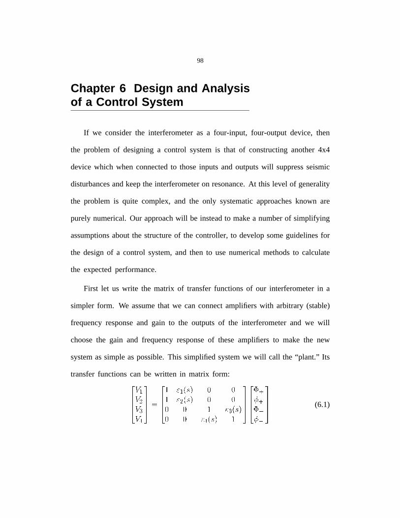
98
Chapter 6 Design and Analysisof a Control System
If we considerthe interferometeras a four-input, four-output device, then
the problem of designinga control systemis that of constructinganother4x4
devicewhich when connectedto thoseinputs and outputswill suppressseismic
disturbancesandkeepthe interferometeron resonance.At this level of generality
the problem is quite complex, and the only systematicapproachesknown are
purely numerical.Our approachwill be insteadto makea numberof simplifying
assumptionsaboutthe structureof the controller,to developsomeguidelinesfor
the designof a control system,and then to usenumericalmethodsto calculate
the expectedperformance.
First let us write the matrix of transferfunctionsof our interferometerin a
simpler form. We assumethat we can connectamplifierswith arbitrary (stable)
frequencyresponseand gain to the outputsof the interferometerand we will
choosethe gain and frequencyresponseof theseamplifiers to make the new
systemassimpleaspossible.This simplified systemwe will call the “plant.” Its
transferfunctionscan be written in matrix form:������������
�
���� �� � � ���� �� � �� � ���� ��� � ���� ��
���� ����� �
(6.1)
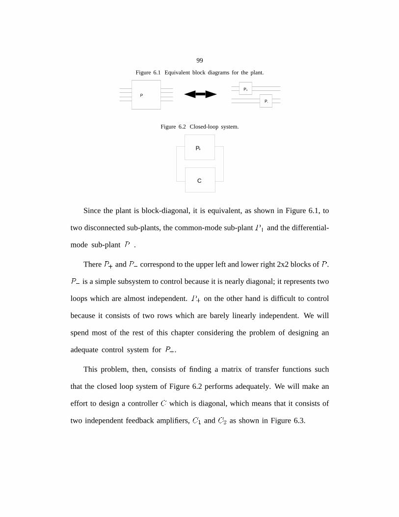
99
Figure 6.1 Equivalentblock diagramsfor the plant.
P
P+
P-
Figure 6.2 Closed-loopsystem.
C
P+
Sincethe plant is block-diagonal,it is equivalent,asshownin Figure6.1, to
two disconnectedsub-plants,thecommon-modesub-plant���
andthedifferential-
mode sub-plant���
.
There���
and���
correspondto theupperleft andlower right 2x2blocksof�
.
���is a simplesubsystemto controlbecauseit is nearlydiagonal;it representstwo
loopswhich arealmostindependent.���
on the otherhandis difficult to control
becauseit consistsof two rows which are barely linearly independent.We will
spendmost of the rest of this chapterconsideringthe problemof designingan
adequatecontrol systemfor���
.
This problem, then, consistsof finding a matrix of transferfunctions such
that the closedloop systemof Figure6.2 performsadequately.We will makean
effort to designa controller � which is diagonal,which meansthat it consistsof
two independentfeedbackamplifiers, ��� and � asshownin Figure6.3.
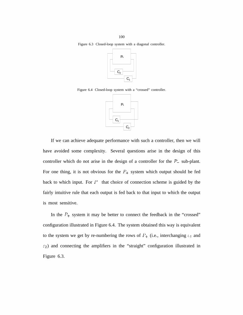
100
Figure 6.3 Closed-loopsystemwith a diagonalcontroller.
P+
C1
C2
Figure 6.4 Closed-loopsystemwith a “crossed”controller.
P+
C1
C2
If we canachieveadequateperformancewith sucha controller,thenwe will
have avoided some complexity. Severalquestionsarise in the design of this
controller which do not arisein the designof a controller for the���
sub-plant.
For one thing, it is not obvious for the���
systemwhich output shouldbe fed
back to which input. For���
that choiceof connectionschemeis guidedby the
fairly intuitive rule that eachoutput is fed backto that input to which the output
is most sensitive.
In the���
systemit may be betterto connectthe feedbackin the “crossed”
configurationillustratedin Figure6.4. Thesystemobtainedthis way is equivalent
to the systemwe get by re-numberingthe rows of���
(i.e., interchanging��� and
� ) and connectingthe amplifiers in the “straight” configurationillustrated in
Figure 6.3.
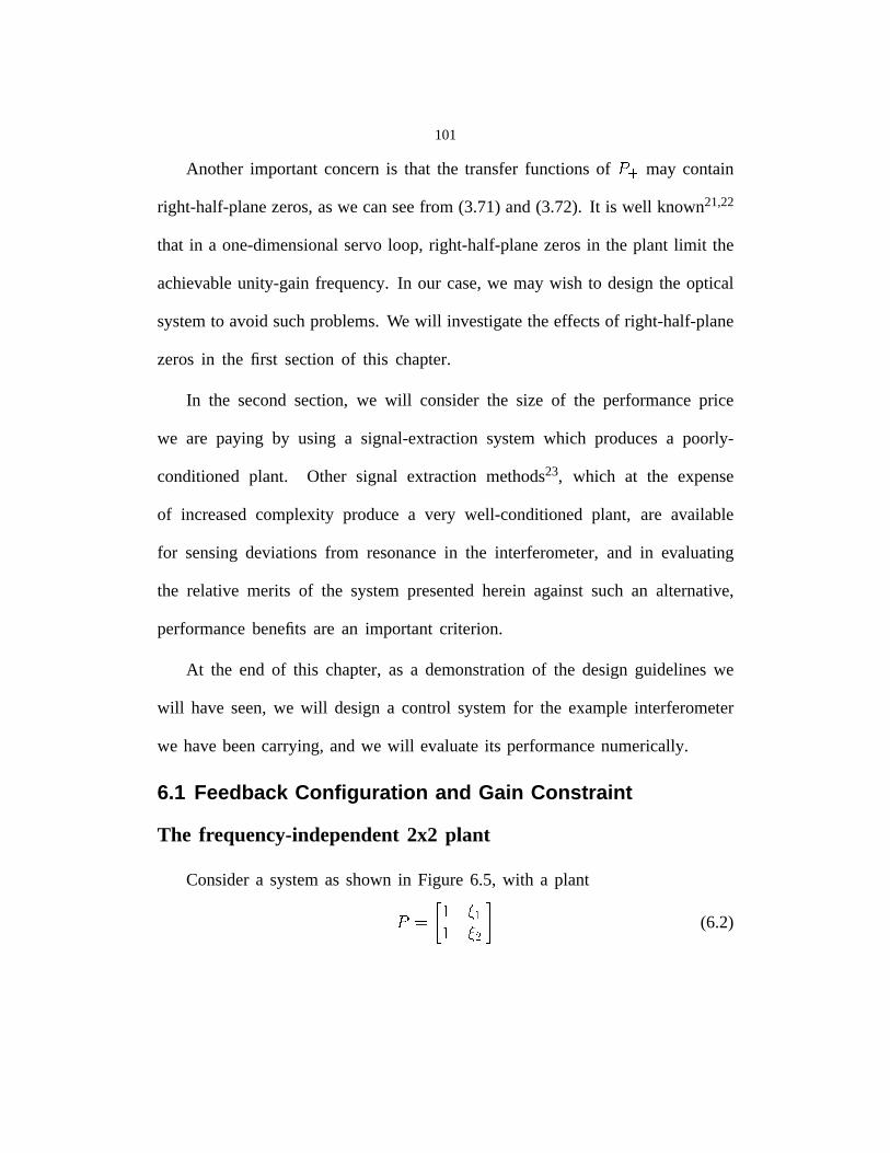
101
Another importantconcernis that the transferfunctionsof���
may contain
right-half-planezeros,aswe canseefrom (3.71)and(3.72). It is well known21,22
that in a one-dimensionalservoloop, right-half-planezerosin the plant limit the
achievableunity-gain frequency.In our case,we may wish to designthe optical
systemto avoidsuchproblems.We will investigatetheeffectsof right-half-plane
zerosin the first sectionof this chapter.
In the secondsection,we will considerthe size of the performanceprice
we are paying by using a signal-extractionsystemwhich producesa poorly-
conditioned plant. Other signal extraction methods23, which at the expense
of increasedcomplexity producea very well-conditionedplant, are available
for sensingdeviationsfrom resonancein the interferometer,and in evaluating
the relative merits of the systempresentedherein againstsuch an alternative,
performancebenefitsare an importantcriterion.
At the end of this chapter,as a demonstrationof the designguidelineswe
will haveseen,we will designa control systemfor the exampleinterferometer
we havebeencarrying,andwe will evaluateits performancenumerically.
6.1 Feedback Configuration and Gain Constraint
The frequency-independent 2x2 plant
Considera systemas shownin Figure 6.5, with a plant
��� � ���� � (6.2)
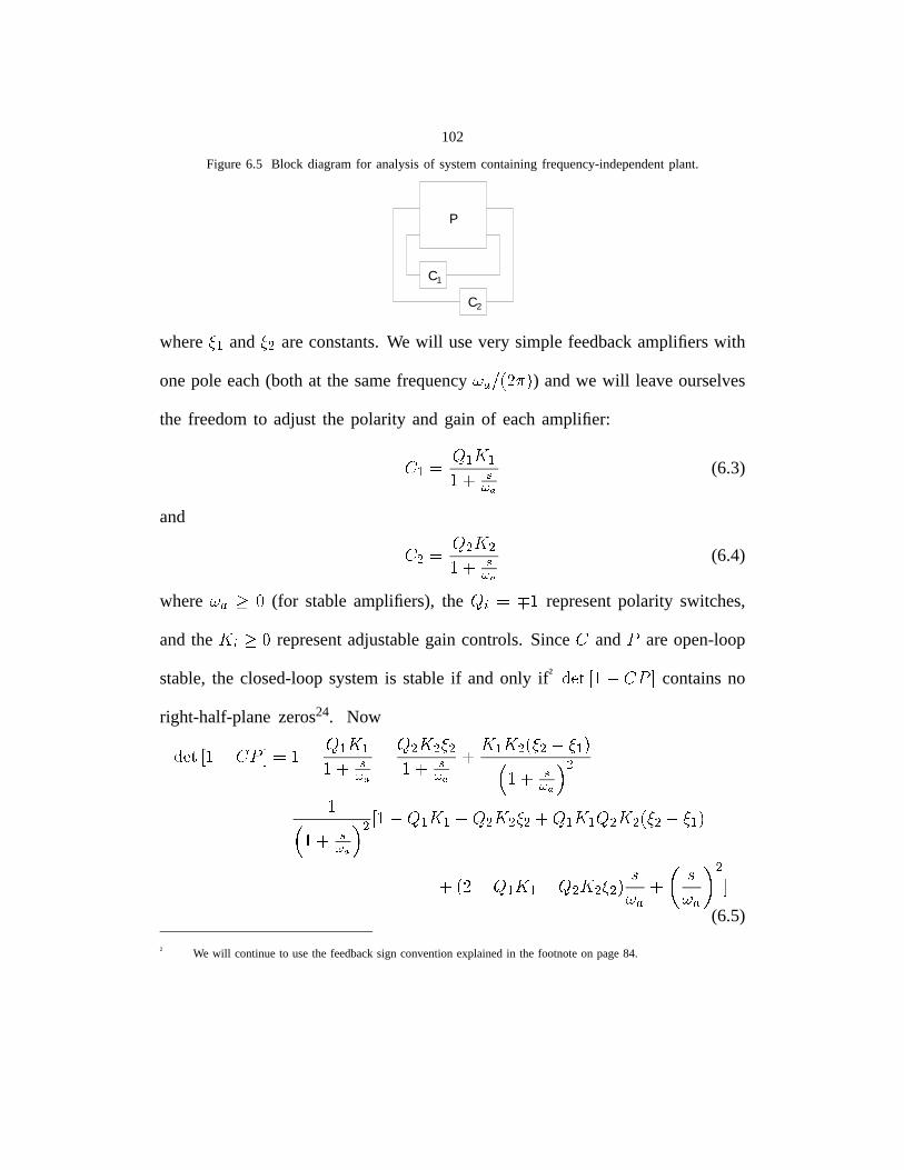
102
Figure6.5 Block diagramfor analysisof systemcontainingfrequency-independentplant.
P
C1
C2
where���
and���
areconstants.We will usevery simplefeedbackamplifierswith
onepole each(both at the samefrequency�������� �� ) andwe will leaveourselves
the freedomto adjustthe polarity and gain of eachamplifier:
� ��� � �������� ���� (6.3)
and
� � � � � � ���� ���� (6.4)
where ��� (for stableamplifiers), the �"! � �representpolarity switches,
andthe� ! representadjustablegain controls.Since
�and # areopen-loop
stable,the closed-loopsystemis stableif and only if† $&%('�) � � #+* containsno
right-half-planezeros24. Now
$,%-'�) � � #.* � � � �-����/� ����
� � � � � ��0� ����� ����� � � � �1� �
�/� �����
� ��0� �� �
� ) � � �(��� � � � � � � � � ����� � � � � � � ��� �
� �� � ����� � � � � � � �"2���� 2���
�*
(6.5)
† We will continueto usethe feedbacksign conventionexplainedin the footnoteon page84.
103
We know that a polynomial with real coefficients has zeroeswith positive
real part if any pair of coefficients hasoppositesigns25 (for a quadratic,it can
be shownthat the latter is also a necessarycondition for the former). The last
coefficient (�����) in thenumeratorpolynomial(in � ) is positive,sofor stability,
all of the remainingcoefficients must be positive.
Now supposewe choose� ��� andwe want to startoff with � ��� � � ���
andthen increasethe gain � � first. If we increaseit to the point where � ���
the systemwill be unstablesince the coefficient of ��� becomesnegative. This
is an undesirablesituation becausewe would prefer to be able to increasethe
gains arbitrarily and enjoy the resulting improvementsin performance. In this
caseit is easyto understandwhat is wrong; asin a one-dimensionalservo,if the
sign of the feedbackis wrong, the systemwill be unstablefor gain exceedinga
certainthreshold.We needto choose� � � to avoid this problem. Similarly
we find that if � ����� then we needto choose� ��� to be allowedarbitrary
� � when � ����� .
We might ask whether thesechoicesof polarity guaranteestability for all
valuesof thegains � � and � � . Theansweris “no”: As we canseefrom the last
coefficient of � � in (6.5), if � � � ����� , the systemis unstableif
� � � ����� � ��� � � � �
� � � � (6.6)
so again the gain is constrainedby stability considerations.It is easyto verify
104
thathadwe numberedour outputsdifferentlywe would havehada stablesystem
no matterwhat(non-negative)valueswe chosefor���
and���
. Equivalently,had
we hookedup the amplifiersin the crossedconfiguration,the correspondingterm
in the � � coefficient would havebeen � � � � and againthe systemwould have
beenstablefor any non-negative���
and��
.
With this motivation, we makethe following
Definition:
The closed-loopsystemconsistingof the plant and two controllers � � ���������������� and � � � ��������������� is gain constrained if � �"! �$# %&! %
suchthatthesystem
is stablefor all positive real valuesof���
and��
.
Now we can show the following:
Theorem 1:
The systemconsistingof the plant �% � �% � � andcontrollers � �'� �(��������)����
and � �*� �+��������)���� connectedin the straightconfiguration is gain constrainedif and
only if
� �-, � � � ��.'/10 (6.7)
Proof:
Sufficiency: � �&, � � � �2.3/40implies either
i. � �6570and � � � �8/70
or
ii. � ��/70and � � � �95:0
105
Casei) is the one we looked at in the exampleand we saw that it is gain-
constrained. In caseii), if we choose����� �
then the term���������
is
negativeand the coefficient of �� becomesnegativefor large��
. If we choose
� � ���, the term
��� � � ����������� ���is negative.
Necessity:If������� �������
we take� � � �
andthe sign of���
opposite
the sign of��
. Then all of the coefficients in the numeratorof (6.5) are non-
negativefor all valuesof� �
and��
.
Frequency-dependent plant
Now we will prove a weakerbut more relevantresult.
Theorem 2:
the systemconsistingof the plant‡
� �� � ��� !#"� �� ��� !%$
(6.8)
and the controllers
& � � � � � ���� !(' (6.9)
and
&��)� ���*����� !('
� (6.10)
‡ +*, canbe written in this form by factoring"" , out of (3.57),(3.61), (3.71),and(3.72).
106
connectedin the straightconfigurationis gain-constrainedif any of the following
is true:
i.��������� ������
ii.��� ���� � ���� � ��
iii. � ����
Proof:
As before, we form
������ � !#"%$'&(� ) �+*,��.- /��0
) ��*1���� �2- /� ��2- /� 0
�
- ) � * � ) � * � � � �.- /� � � � �2- /� ��.- /� 0
3
& ��.- /� 0
3 �4� ) �5*,� ) ��*1�6��� - ) �7*,� ) ��*1�8����� �8� $
-9�;: < ) �5*,� ) ��*1���� �.- ��=� �
- ) �5*,� ) ��*1� ��=� �� �
� �� � $ >
� =- : ) �5*,� ) ��*1�6��� ��=
� � >��=
�- >
��=3
(6.11)
Now it is easyto seethat if anyof theconditionslisted in the theoremholds,
thenat leastoneof thecoefficientsof*,�
,*1�
, or*,�7*1�
will be negativeandthe
systemwill be unstablefor somevaluesof thesegains.
107
Implications for the Interferometer
Becauseof the way in which we numberedthe interferometeroutputs,the
feedbackconfigurationof Figure1.7 correspondsto the straightconfigurationfor
���. In Chapter7 wewill seethatthishasanimportantadvantageoverthecrossed
configuration(with the samenumbering). We let
��� ��� �� ��������� ��� ��������� �� (6.12)
Substitutingfrom (2.77), (2.78), (3.57) and (3.72), we get
�������! " �! �� " # $ " (6.13)
and
����� � � "� � $�$ (6.14)
Similarly, letting
�&% ��� %� �(')��� � ��� � ' � � � �� (6.15)
and using (2.70), (2.74), (3.61), and (3.71), we have
�*%+��� " � �� " # $ " (6.16)
and
%+��� � � "� � $�$ (6.17)
Now the necessaryconditionsfor freedomfrom gain constraint(Theorem2)
become:
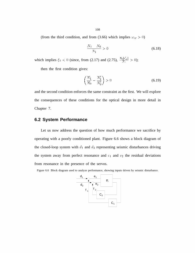
108
(from the third condition,and from (3.66) which implies ��������� )� ���� ��� (6.18)
which implies ��� � � (since,from (2.17) and (2.75), ����� ���� � ������� );
then the first condition gives:
� � �
���� �� ��� (6.19)
andthesecondconditionenforcesthesameconstraintasthefirst. We will explore
the consequencesof theseconditions for the optical design in more detail in
Chapter7.
6.2 System Performance
Let us now addressthe questionof how much performancewe sacrificeby
operatingwith a poorly conditionedplant. Figure6.6 showsa block diagramof
the closed-loopsystemwith and !� representingseismicdisturbancesdriving
the systemaway from perfect resonanceand " and "�� the residualdeviations
from resonancein the presenceof the servos.
Figure6.6 Block diagramusedto analyzeperformance,showinginputsdriven by seismicdisturbance.
P+
d2
d1
C1
C2
e1
e2
f 1f 2
109
We solve for�� :
�������� �� (6.20)
�� � �� � ��(6.21)
�� ����� �������� ��(6.22)
If we let
� ��� ���������(6.23)
then
��� ��� � � � � ��� ��� � � (6.24)
We will considerthis term first.
The smaller � � is, the bettera job our control systemis doing. Clearly the
larger we can make the elementsof�
, the better. In a real systemthere are
alwaysaspectsof the high frequencyperformanceof the systemwhich limit the
unity-gain frequencyand therebythe gain one can achieveat thosefrequencies
whereonewantsto suppressdisturbances.In our system,assumingthatit is not in
a gain-constrainedconfiguration,thesehigh frequencyfeatureswill bemechanical
resonancesat about 10 kHz for any loop driving a mirror, and propagation
delays in the optical path and wiring, which producesignificant phasedelays
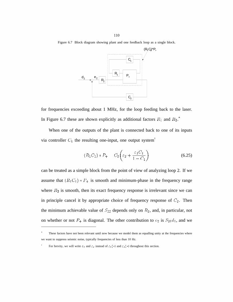
110
Figure 6.7 Block diagram showing plant and one feedback loop as a single block.
P+
C1
R2
C2
R1d2 e2
(R C)*P1 +1
for frequencies exceeding about 1 MHz, for the loop feeding back to the laser.
In Figure 6.7 these are shown explicitly as additional factors���
and���
.*
When one of the outputs of the plant is connected back to one of its inputs
via controller � �the resulting one-input, one output system†
� � � � ��� � � � � ����� ��� � �� � � (6.25)
can be treated as a simple block from the point of view of analyzing loop 2. If we
assume that� � � � ��� �
is smooth and minimum-phase in the frequency range
where� �
is smooth, then its exact frequency response is irrelevant since we can
in principle cancel it by appropriate choice of frequency response of � �. Then
the minimum achievable value of � ���depends only on
� �, and, in particular, not
on whether or not�
is diagonal. The other contribution to � � is � �������, and we
* These factors have not been relevant until now because we model them as equalling unity at the frequencies where
we want to suppress seismic noise, typically frequencies of less than 10 Hz.
† For brevity, we will write ��� and ��� instead of ��� �"!$# and ���%�&! # throughout this section.
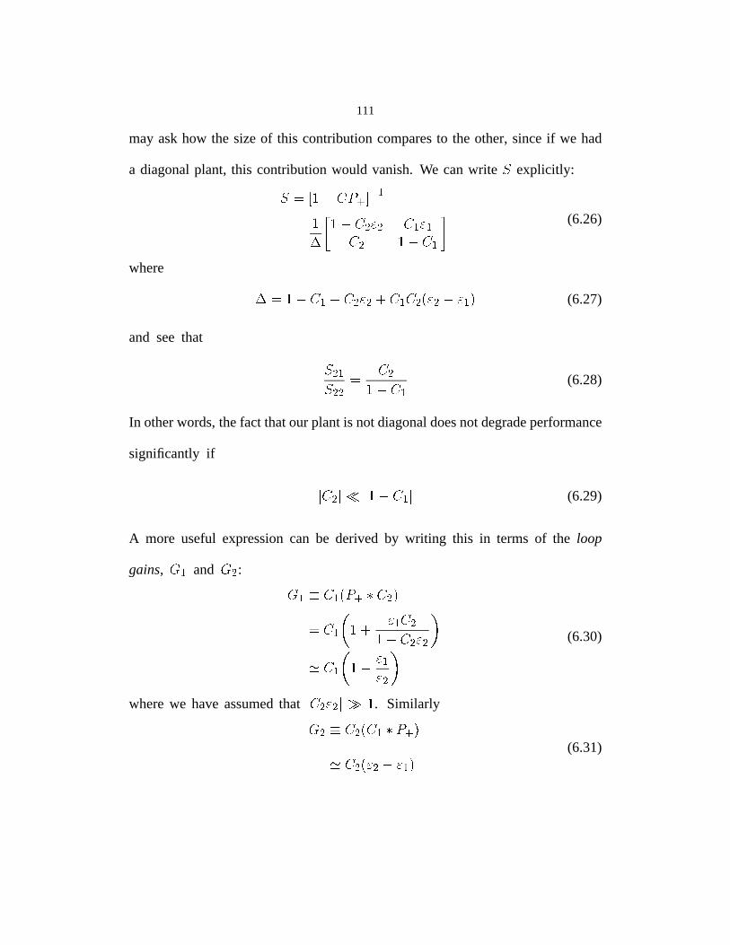
111
may askhow the sizeof this contributioncomparesto the other,sinceif we had
a diagonalplant, this contributionwould vanish. We canwrite�
explicitly:������� ������ ��� ��
� ������� � � � ���� � � �(6.26)
where
����� � � ����������� � ��������� � �! (6.27)
and see that
�"� ��"�#� ����
� � � (6.28)
In otherwords,thefact thatourplantis notdiagonaldoesnotdegradeperformance
significantly if
��� � � � (6.29)
A more useful expressioncan be derived by writing this in terms of the loop
gains, $ � and $ � :$ � � � �%�� ���
�&� � �'� � � ���� ���!���� � � � ����
(6.30)
wherewe haveassumedthat������� �
. Similarly
$ � �����%� � �� �����(��� � ��
(6.31)
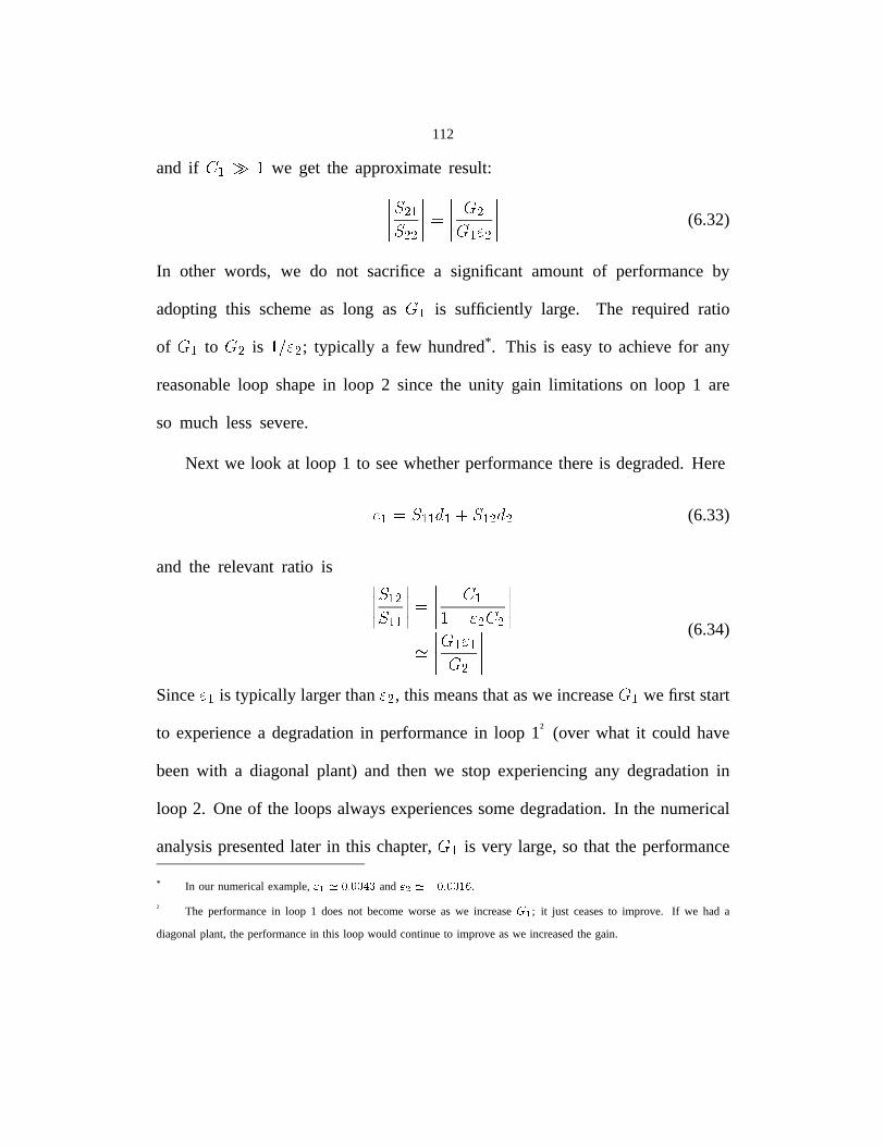
112
and if��� �
we get the approximateresult:
���������
���� ����� (6.32)
In other words, we do not sacrifice a significant amount of performanceby
adopting this schemeas long as� �
is sufficiently large. The required ratio
of� �
to���
is�������
; typically a few hundred*. This is easyto achievefor any
reasonableloop shapein loop 2 since the unity gain limitations on loop 1 are
so much less severe.
Next we look at loop 1 to seewhetherperformancethereis degraded.Here
� � ��������������������(6.33)
and the relevant ratio is���������
���� ��� �!�� � � ����
(6.34)
Since�"�
is typically largerthan���
, this meansthataswe increase� �
we first start
to experiencea degradationin performancein loop 1† (over what it could have
beenwith a diagonalplant) and then we stop experiencingany degradationin
loop 2. Oneof the loopsalwaysexperiencessomedegradation.In the numerical
analysispresentedlater in this chapter,�#�
is very large, so that the performance
* In our numericalexample,$&%('*)�+ ),).-&/ and $.01'32 )�+ ).)465 .† The performancein loop 1 doesnot becomeworse as we increase7�% ; it just ceasesto improve. If we had a
diagonalplant, the performancein this loop would continueto improveaswe increasedthe gain.
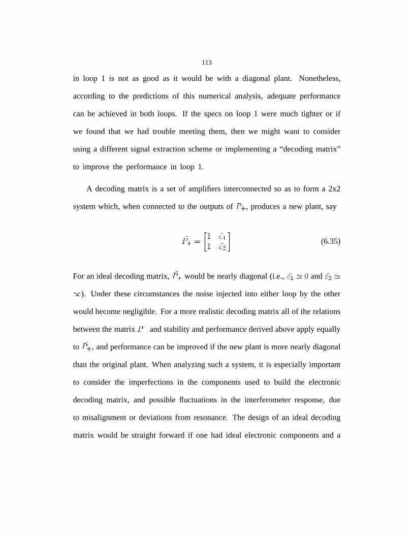
113
in loop 1 is not as good as it would be with a diagonalplant. Nonetheless,
accordingto the predictionsof this numerical analysis,adequateperformance
can be achievedin both loops. If the specson loop 1 were much tighter or if
we found that we had trouble meetingthem, then we might want to consider
using a different signal extractionschemeor implementinga “decodingmatrix”
to improve the performancein loop 1.
A decodingmatrix is a set of amplifiersinterconnectedso as to form a 2x2
systemwhich, whenconnectedto the outputsof���
, producesa new plant, say
������ � ��� ���� (6.35)
For an idealdecodingmatrix,����
would benearlydiagonal(i.e.,�� and
����
). Under thesecircumstancesthe noise injected into either loop by the other
would becomenegligible. For a morerealisticdecodingmatrix all of therelations
betweenthematrix���
andstability andperformancederivedaboveapplyequally
to����
, andperformancecanbe improvedif thenewplant is morenearlydiagonal
thanthe original plant. Whenanalyzingsucha system,it is especiallyimportant
to consider the imperfectionsin the componentsused to build the electronic
decodingmatrix, and possiblefluctuationsin the interferometerresponse,due
to misalignmentor deviationsfrom resonance.The designof an ideal decoding
matrix would be straight forward if one had ideal electroniccomponentsand a

114
non-varyinginterferometerresponse;a real devicewith imperfectionsmay yield
smaller performancebenefits.
6.3 Numerical Example of a Control System Design
Mainly for the sake of illustrating some of the ideas developedabove, a
controller was designedand evaluatednumerically*. The designwas done by
trial anderror. Polesandzeroswereaddedto thecontrollerandtheir frequencies
changeduntil adequateperformancewas achievedand all of the constraints
satisfied.The polesandzerosof the final design†26, aswell as the performance
predictedfor this design,are shownin Table 6.1.
Simplenumericalmodelswereusedto representthe plant andthe controller.
For theplant, the rationalfunctionapproximationderivedin Chapter3 wasused;
for thecontroller,a rationalfunction(pole/zero)representationwasused.Thusthe
numericalmodeldid not containthe effect of internal resonancesin the mirrors,
nor the effect of propagationdelays. That theseunmodeledeffects would not
causeinstability in a real systemwas checkedby inspectionduring the design
process.
* Almost all of the analysisdescribedin this sectionwasdoneusingMatlab code.
† L. Sieversfirst observedthat adequateperformancecould be achieved,and all of the designconstraintssatisfied,
with controllerscontainingonly real polesandzeros(i.e., no complexconjugatepairsof polesor zeros).
115
Constraints
Stability As mentionedabove,a mirror resonancecould causeinstability if the
loop gain at the resonantfrequencywere to exceedunity. Sincethe resonances
are expectedto havequality factorsof up to 107 and are expectedto occur at
frequenciesaslow as10 kHz27, this type of instability wasruled out by assuring
that the magnitudeof the loop gain in any of the loopsdriving a mirror wasless
than 10–7 at frequenciesexceeding10 kHz*28.
In the loop feeding back to the laser frequencythe criterion was simply
that the unity gain frequencybe less than 1 MHz. At that frequency80 ns of
delay(correspondingto 24 m of optical path),togetherwith 15 degreesof phase
changeseenin the high frequencyinterferometerresponse(H_11 of Figure4.2),
still leavesa phasemargin of up to 70 degrees.
The simplified rational function modelof the closedloop systemcould also
be unstableby itself. This was checkedby finding the eigenvaluesof the “A”
matrix in the state-spacerepresentation† of the closed-loopsystem,to makesure
that their real parts were positive.
Noise Oneadditionalconstraintwasobservedduring the design.As we sawin
Chapters2 and3, the gravitationalwaveoutput,in additionto beingsensitiveto
* A Mathematicaprogramwas written to checkthis particularconstraint. This was necessarybecausethe Matlab
code,usingthe state-spaceformalism,underestimatedthe attenuationat high frequencies.
† The (Matlab) softwareusedto do this part of the analysisanddesigndoesall of its calculationsin statespace.
116
���, is alsosensitiveto � � . If � � is controlledby a loopcontaininganoisysensor,
thenthe inducednoisein � � will contaminatethe gravitationalwavesignal*.
Quantitatively, we require, at frequencieswhere we want interferometer
performanceto be limited only by shotnoiseat the antisymmetricoutput (above
100 Hz),
��� ��� ������� � � ���� � � ������� ����� (6.36)
where ��� � ����� and ��� � ����� are the shot-noiselimited sensitivity to � � at the
isolatorandto� �
at the antisymmetricoutput,and � � � is the open-loopgain in
the � � loop. In our numericalexample,this correspondsto
� � � � � � (6.37)
and we use � � �"!#�$�%� � as our constraint.
Performance
Figure6.8showstheexpectedseismicdisturbancedriving eachof theinterfer-
ometermirrors†29. To calculatethe rms deviationfrom resonance,this spectrum
is first multiplied by a number &(' correspondingto the numberof mirrors being
* In principle, this noise,being separatelymeasurablein the ) � loop, could be subtractedout of the gravitational
wavesignal. However,theprecisionwith which this canbedoneis limited by practicalconsiderations,andtheadditional
complexity is undesirable.
† This curvewascalculatedfrom a combinationof estimatedandmeasuredspectraof the seismicmotion, and from
the transferfunctionsof the mechanicalanti-seismicisolation.
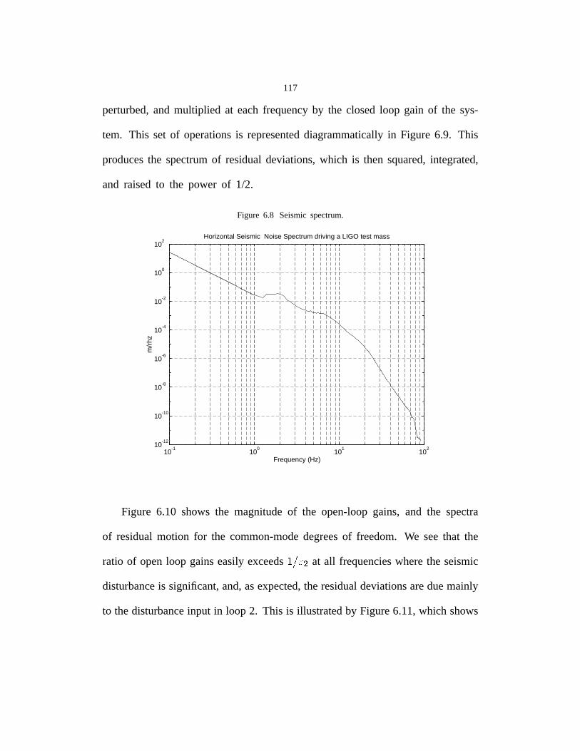
117
perturbed,and multiplied at eachfrequencyby the closedloop gain of the sys-
tem. This set of operationsis representeddiagrammaticallyin Figure 6.9. This
producesthe spectrumof residualdeviations,which is then squared,integrated,
and raisedto the power of 1/2.
Figure 6.8 Seismicspectrum.
10-1
100
101
102
10-12
10-10
10-8
10-6
10-4
10-2
100
102
Frequency (Hz)
m/r
hz
Horizontal Seismic Noise Spectrum driving a LIGO test mass
Figure 6.10 shows the magnitudeof the open-loopgains, and the spectra
of residualmotion for the common-modedegreesof freedom. We seethat the
ratio of openloop gainseasilyexceeds�������
at all frequencieswherethe seismic
disturbanceis significant,and,asexpected,theresidualdeviationsareduemainly
to thedisturbanceinput in loop 2. This is illustratedby Figure6.11,which shows
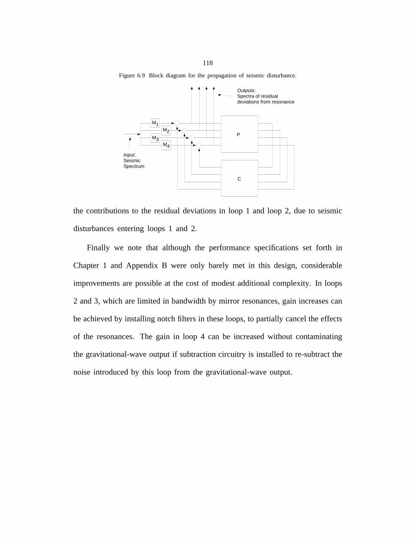
118
Figure 6.9 Block diagramfor the propagationof seismicdisturbance.
M1M2
M3M4
P
C
Input: Seismic Spectrum
Outputs: Spectra of residual deviations from resonance
the contributionsto the residualdeviationsin loop 1 and loop 2, due to seismic
disturbancesenteringloops 1 and 2.
Finally we note that although the performancespecifications set forth in
Chapter1 and Appendix B were only barely met in this design,considerable
improvementsarepossibleat the costof modestadditionalcomplexity. In loops
2 and3, which arelimited in bandwidthby mirror resonances,gain increasescan
beachievedby installingnotchfilters in theseloops,to partially canceltheeffects
of the resonances.The gain in loop 4 can be increasedwithout contaminating
thegravitational-waveoutputif subtractioncircuitry is installedto re-subtractthe
noiseintroducedby this loop from the gravitational-waveoutput.
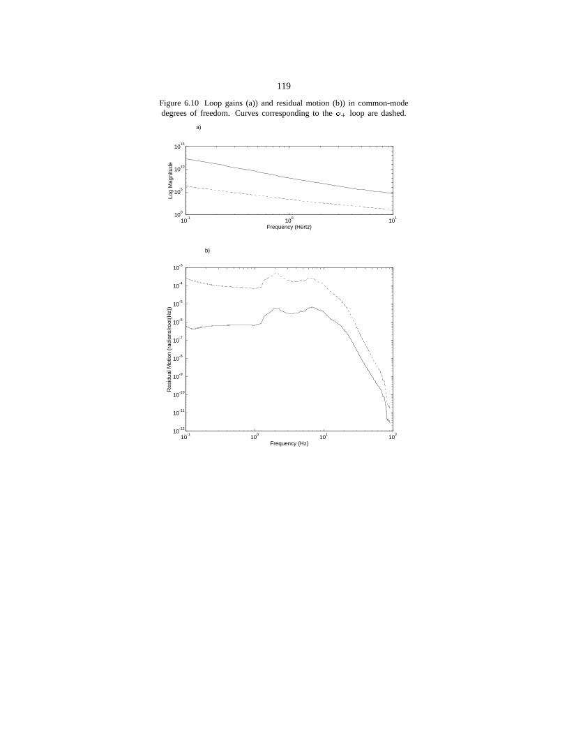
119
Figure 6.10 Loop gains (a)) and residual motion (b)) in common-modedegrees of freedom. Curves corresponding to the
���loop are dashed.
10-1
100
101
100
105
1010
1015
Frequency (Hertz)
Log
Mag
nitu
de
a)
10-1
100
101
102
10-12
10-11
10-10
10-9
10-8
10-7
10-6
10-5
10-4
10-3
Frequency (Hz)
Res
idua
l Mot
ion
(rad
ians
/roo
t(H
z))
b)
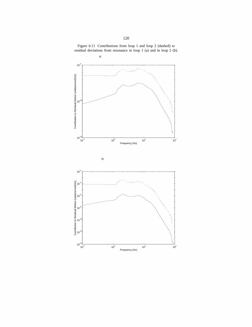
120
Figure 6.11 Contributions from loop 1 and loop 2 (dashed) toresidual deviations from resonance in loop 1 (a) and in loop 2 (b).
a)
b)
10-1
100
101
102
10-15
10-10
10-5
Frequency (Hz)
Con
trib
utio
n to
Res
idua
l Mot
ion
(rad
ians
/roo
t(H
z))
10-1
100
101
102
10-14
10-12
10-10
10-8
10-6
10-4
10-2
Frequency (Hz)
Con
trib
utio
n to
Res
idua
l Mot
ion
(rad
ians
/roo
t(H
z))
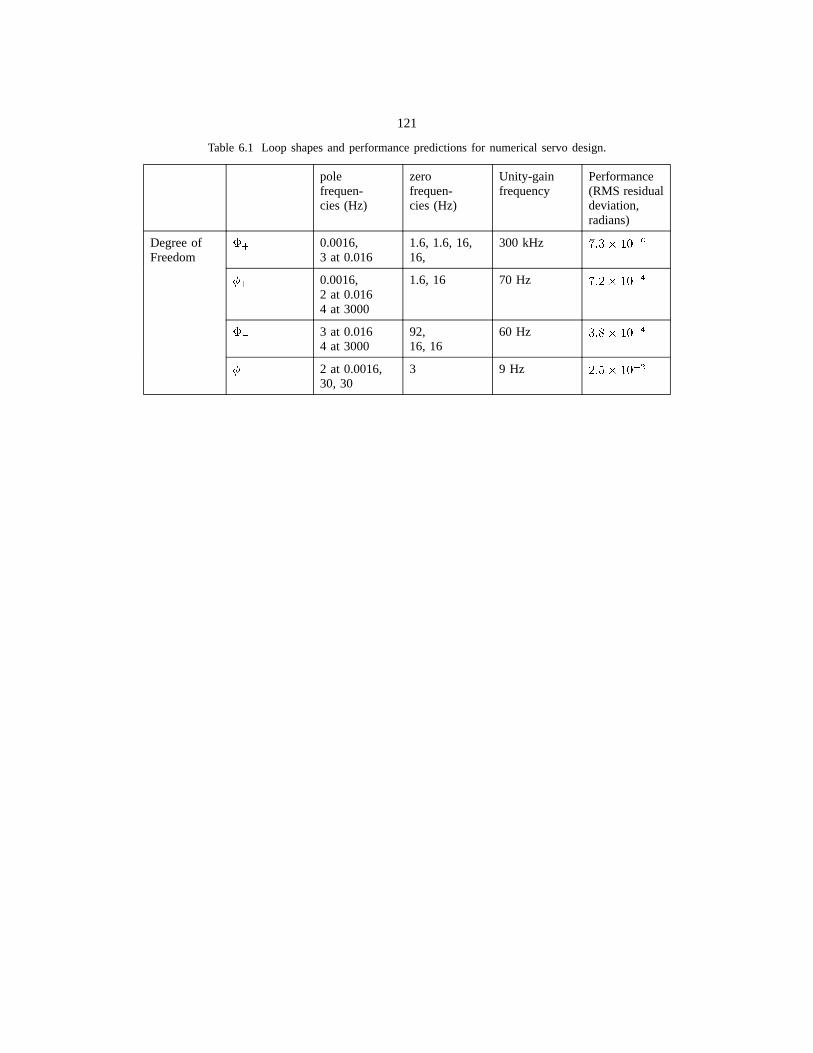
121
Table 6.1 Loop shapes and performance predictions for numerical servo design.
polefrequen-cies (Hz)
zerofrequen-cies (Hz)
Unity-gainfrequency
Performance(RMS residualdeviation,radians)
Degree ofFreedom
� 0.0016,3 at 0.016
1.6, 1.6, 16,16,
300 kHz �
�
� 0.0016,2 at 0.0164 at 3000
1.6, 16 70 Hz �
�
�3 at 0.0164 at 3000
92,16, 16
60 Hz �
�
�2 at 0.0016,30, 30
3 9 Hz �
�
122
Chapter 7 Optical Design Considerations
In previous chapters,a number of somewhatarbitrary choicesof optical
parametersand layout have been made. In this chapterwe will investigate
the motivation behind someof thosechoices. In particular, we will consider
the choiceof common-modefeedbackconfiguration,of asymmetry,of recycling
mirror reflectivity, and of modulationdepth.
7.1 Common-mode Feedback Configuration
In Figure 1.7 we showedthe feedbackto the laser frequencycoming from
the isolatorinphaseoutputandthe feedbackto the recyclingmirror positionfrom
the pick-off inphaseoutput. In principle onecould reversetheseconnectionsfor
someoptical configurations. One compelling reasonto feed back to the laser
frequencywith ��� is that the shot-noiselimited sensitivity to���
, is betterin ���
thanin ��� (typically by a factorof about30). Sincewe insist on high gain in this
loop, any sensingnoise in this loop will be impressedon the laser frequency*.
This noisecan be measured,and it could in principle be subtractedout of the
gravitationalwave signal, but this is technically difficult, and would require a
separatelow-noise frequencyreference†.
* Although thegravitationalwaveoutputof an ideal interferometeris insensitiveto � , a smallasymmetryin thearm
cavitiescancompromisethis common-moderejection.
† The currentlyproposedmodecleaner(seefootnote,page8) is almostquiet enough,andcould be madesufficiently
quiet by narrowingits bandwidth.
123
7.2 Asymmetry
An immediateconsequenceof this choiceof feedbackconfigurationis that
(accordingto (6.18)) avoiding gain constraintwill require
��� ������ ��� (7.1)
which implies (using (2.71) and (2.75))
� ��� ����� � (7.2)
A numberof other aspectsof interferometerbehaviorare affectedby the value
we choosefor theasymmetry� . Oneof theseis the shot-noiselimited sensitivity
in ��� to ��� , the gravitationalwave signal:
�����! #"%$'&�)(+*%(+* ",$)&
- ( * �! "/.,0213$4& (7.3)
where
� ( * ( * ",$4&65 7�8%9 � 8,:,: ;=<?> 7A@CB�DFE � ; (7.4)
and
- (+* � 5G7 ;HJI � "LKM& I � "%KM& 7AN �7AEOB � �
7A@PB�DFE �7QEOB � � RTSU�WV� � (7.5)
Theaboveexpressionis complicatedandits optimizationis usuallydonenumeri-
cally. However, � affectsonly theterm > 7A@PB�DXE � ; in thenumeratorand Y[Z%\^]`_ �Y _a\cb �in the denominator.The numeratorincreaseswith 7A@PB�DFE � moreslowly thandoes
124
the denominator,so increasing���������� ����� improvesthe shot-noiselimited sensi-
tivity to���
. Now�������������������
�! �"$#% &('*),+.-0/ �1# (7.6)
is maximum when
-2/ �1#43 &('*),+(7.7)
which correspondsto # 57698 in our numericalexample.However,the following
considerationsmotivateus to choosea smallervalue for # :
1. The vacuumenvelopemustbe able to accommodatethe test masspositions
correspondingto the desiredasymmetry.This may be easierwith a smaller
value of : .2. The shot-noiselimited sensitivity to
�<;in = � is degradedif the amountof
sidebandreflectedfrom the recycling mirror�?>A@ABC� �D�E�F is too small. From
(2.77) we can see that in fact the signal will vanish when�?>G@�B1� ���E�F 3H5 ,
which happenswhen-2/ �1#I3KJMLNPO , a value uncomfortablycloseto the value
in (7.7) above.
3. As mentionedabove,if we wish to be free from gain constraint,we must
choose-/ ��#RQ & �TS
; moreover,we will seein the next sectionthat we wish
to choose&(' & �TS
, so againthis motivatesthe useof a smallervalueof # .
4. The shot-noiselimited sensitivityto���
is quite a weakfunction‡ of # . This
‡ A numericalsurveyovera largerangeof valuesfor contrastdefect,recyclingmirror transmissionandlossesshowed
that the shotnoiselimited sensitivity to gravitationalwaveswasdegradedby at most5% when U wasreducedto 0.15.
125
is becausea lack of efficiency in transmissionto the antisymmetricport can
be partially compensatedby an increasein the modulationindex.
Fromtheaboveargumentsweconcludethatthechoiceof � is not critical, and
we chooseone which is roughly 75% of the value which would give optimum
shot noise performance.
7.3 Recycling Mirror Reflectivity
Therecyclingfactor (seefootnote,page26) is maximumfor ����� ��� ��� , and
we would like to operateas closeas possibleto this value. Beforechoosing� �we will makesurethat condition (6.19) is not violated.
�� �
��� ��
��� (7.8)
implies
� � � ��� ����� � ��������� � ��� (7.9)
which is satisfiedif
� �!� � � ���� (7.10)
But we have alreadychosento satisfy this in Section7.2, in order to achieve
"$# ��� (no right-half-planezeroin %'&)(+*�,.-0/21 ). Wearefreeto chooseanyrecycling
mirror reflectivity we want. It is interestingto note that this would not be the
casewerewe to demandthat %'& 3�*,.-0/�1 alsobe free of right-half-planezeros.
126
7.4 Modulation Index
The shot noise limited gravitationalwave sensitivity of the instrumentis a
relatively sensitivefunction of the modulationindex�
, especiallyif ���������� is
large, and for large ���������� the optimum value of�
is also large. For large�
the approximation(2.2) is no longer valid, and one needsto add (at least) an
additional pair of terms:
�� ���� ��� ����� ����� ����� ��� ��� ! #" �$����% ! &" ��'�� ��� � !'( &" �)��% *'+ &"(7.11)
Wecall thefrequencycomponentsseparatedfrom theopticalcarrierby ,�- second-
order RF sidebands; they arereflectedalmostperfectlyfrom the recyclingmirror
�/. ��01'�� !���&'
2(7.12)
since(by design)* they do not resonatein the arm cavitiesnor in the recycling
cavity. They arecapableof beatingagainstthe first-orderRF sidebandsto create
a signal at the mixer output. Generalizing(2.4):
3�46587 � �:9% ' � % � � �;9% � �/� � �:9� �<� � �;9� ��' (7.13)
If � % ' 5 ��' andthesefields aswell as �/� arereal, and if � % � 5 �<� then
3 4 5 , 7 � �<������� � �=' � (7.14)
Thefieldsat the isolatorsatisfytheseconditions,andtheaboveexplanationholds
for 3 � , the inphasesignal at the isolator. We seethat the signal generatedin 3 �* Seefootnotepage27.
127
whenthe carrierphasechangesis unaffectedby the presenceof the second-order
sidebands,so that������������
is unaffected by the presenceof the second-order
RF sidebands.The contributionto�������������
due to the changein phaseof the
first-ordersidebandsis affected,however; the size of this contributionchanges
by a factor*
������������ ��� � ��� �"! �
� � �#! � (7.15)
This contributionremainsfrequencyindependent,sincethesignalis dueto audio
sidebandson the first-order RF sidebands,and we accountfor it by defining$%'& � ��(*),+.-0/( )1+.-32 %54&
and replacing%64&
by$%7&
in all of our formulae. In
particular, (7.9) becomes
8�9 :<;=8�> �8�9 : ;@?BADCFE � � � � �#! �
� � �#! � G � (7.16)
Using (7.11), (7.12) and (2.38), we find
� � �#! �� � �#! �
H=�I�JK HD�D�JK � 8�9K: ; 8 > �
8�9 : ; 8 > � (7.17)
Now if (motivatedby the argumentsin Section7.2) we have 8�9 :<; ?LADCME GONthen regardlessof whether 8�9 : ; 8 > � is positive or negative†, (7.16) is harder
to satisfy than (7.10).
* The fields P / and P�Q / areunaffectedby the phasesin the interferometersincethey do not resonatein it.
† Thesetwo casescorrespondto havingthecarrierbe “undercoupled”or “overcoupled,”respectively,at therecycling
mirror.
128
A sufficient condition for this effect to be small is
�������������� �
� �������� ������� ������������� �! �"���#�$����� � % (7.18)
or
� �#����� &(' )+*�&$, �% & ' )-*�&(, � (7.19)
Thiseffectof thesecond-orderRFsidebandsis inconvenientbecauseit implies
that the frequencyresponseof the interferometerdependson modulationindex.
Increasingthe modulationindex to optimize the sensitivitywill requirenot only
adjustingthe servogainsto compensatefor the changein overall response,but
will carry a risk of significantly degradingthe control systemperformance.
Onesolution,althoughitself inconvenient,is to amplitudemodulatethebeam
at .#/ before or after the phasemodulation occurs‡. If properly tuned, the
sidebandsappliedthis way will exactlycancelthosedueto thephasemodulation.
Another potential solution is to arrangethe arm cavity lengthsso that the
second-orderRF sidebandsare exactly resonantin the arm cavities. This possi-
bility hasnot beeninvestigatedin any detail.
‡ If an electro-opticmodulator is usedas the power-stabilizingfeedbackelement,then a convenientand power-
efficient way to apply this modulationwill be to insert an additional crystal driven at 0�1 betweenthe polarizers,or
to sum the power stabilizerand 021 signalselectronicallybeforeapplying them. A stand-aloneamplitudemodulatoris
power-inefficient becausethe beammustbe attenuatedto someextentfor the modulatorresponseto be quasi-linear.
129
7.5 Arm Cavity and Recycling Cavity Lengths
The arm cavity lengthwhich is easiestto analyzeis one for which the first-
order RF sidebandsare exactly antiresonant,i.e., a length of ������ ������ with
� a whole number. In this casethe sidebandsexperienceno phasechangeupon
reflectionfrom the arm cavitiesandthe averagelengthof the recyclingcavity is
chosento be � �� � ����� . Thenwhenthe carrier resonatesin all threecavities,
the sidebandsresonateonly in the recyclingcavity30. This configurationhasthe
disadvantagethat it allows the second-orderRF sidebandsto resonatein all three
cavitiesaswell, making the responseof the interferometerharderto understand,
andverysensitiveto smalldeviationsfrom thesedesignlengths.For this reason,in
our numericalexamplethearmcavity lengthswerechosento beslightly different
from thosewhich would makethe first-orderRF sidebandsexactlyantiresonant.
It is alsopossibleto usevirtually arbitraryarm cavity lengths,so long asthe
first-orderRF sidebandsdo not resonate§|| in the arm cavities. However, if the
sidebandsarefar from beingantiresonantin eitherarm,thentheywill experience
significantphasechangesuponreflectionfrom thatarm,andtheaveragerecycling
cavity length as well as the asymmetrymust be adjustedto compensatefor this
phase.
§ If the sidebandsresonatein the arm cavities,then the RF sidebandphasebecomesquite sensitiveto ��� and the
plant becomesmore ill-conditioned.
|| To avoidanexaggeratedsensitivityto alignmentit is alsoimportantto avoidallowing thesidebandsto fall onto the
resonantfrequencyof other low-order transversemodes.
130
Chapter 8 Summary and Conclusion
Whenthesystemfor extractingsignalsdescribedhereinwasfirst conceived,a
numberof concernsexistedaboutwhethertheasymmetriclayoutwouldfit into the
proposedvacuumsystem,whetherthe asymmetrywould causeexcessivelosses
becauseof thedifferentmode-matchingdemandsimposedby thetwo arms#31, how
the systemwould respondto imperfectionsin the optical componentsor in their
alignment,andwhetherit would be possibleto acquirelock with sucha system.
In addition,it wasunclearwhetherthefact thattwo of theoutputsareproportional
to barely independentlinear combinationsof two of the degreesof freedom(that
the plant is ill-conditioned)would proveto be a formidabletechnicalproblem.
Since then, a numberof theseissueshave becomebetter understood. An
experimentalprototypehasdemonstratedthat,at leastfor aparticularsetof optical
parameters,the assumptionsmade in constructinginterferometermodels have
beenreasonable.The issueof whetherit is possibleto control the ill-conditioned
systemadequatelyhas beenresolved. The performancesacrificesinvolved are
understood,and the constructionof a working prototypeis further evidencethat
this problemis not critical. The dynamicsof the interferometerarealsobelieved
fairly well understood.Theapproximateresultsfrom a simpleanalysisagreewell
with an independentlyassemblednumericalmodel, and both predict behavior
# A. Abramovici hassinceshownthat this effect is completelynegligible.
131
which is simpleenoughnot to requireadditionalcomplexity from the controller.
Optical configurationscorrespondingto a plant which is hard to control have
beenidentified, and are easily avoided.
Other issuesremain less well settled. The following sectionsdescribea
numberof such issues.
8.1 Robustness
Although the prototype interferometerdescribedin chapter5 showed,for
one geometryand set of optical parameters,that the systemis not dangerously
sensitive to imperfections,very little was done to quantify the magnitudeof
the imperfectionsexisting there,and in any case,it would be difficult to make
predictionsfor the behaviorof a full-sized interferometerthis way. In its full
generality,the issueof interferometerbehaviorin the presenceof imperfections
is very complicated.However,with a combinationof analysisof imperfections
perceivedas likely to causetrouble, and careful prototyping, the risk that an
importantproblemmaysurfacevery latecanbereduced.Oneareawhich remains
largely unexploredconcernsrobustness.This is loosely definedas the ability
of a control systemto maintain good performancein the presenceof various
imperfections. Theseimperfectionscan include differencesbetweenactualand
ideal mirror reflectivities, misalignment,imperfectionsin electroniccomponents,
andeventhe effect on the interferometerresponseof deviationsfrom resonance.
132
Both experimentalprototypingandnumericalanalysisarepowerful methods
for testing robustness. The former automatically tests for the simultaneous
effect of a large numberof imperfections,whereasthe latter permitsa carefully
controlledcalculationof the effect of a relatively small numberof imperfections.
The systempresentedhereinmay merit someadditionalnumericalinvestigation
beforethe next stageof prototypingis attempted.Sometypesof imperfections,
which arelikely both to occurandto affect systemperformance,arelistedbelow.
Beam Splitter Reflectivity
Even with today’s bestcoating techniquesit is difficult to producea beam
splitter having a reflectivity differing by less than about5% from the specified
value of 50%. Consequentlythe RF sidebandssamplethe lengths���
and���
in different proportions; the effective averagerecycling cavity length and the
effective asymmetry � are both affected. The effect of an asymmetricbeam
splitter canbepartly cancelled32 by anappropriatemodificationof���
and���
; this
hasbeencheckedin a limited numberof numericaltests.
Mixer PhaseErr or
In our modeleachmixer is driven by a local oscillatorsignalwhich is either
exactlyin phasewith thephasemodulatingsignalor exactlyin quadraturephase.
In a real interferometer,thesephaseswill be affectedby propagationdelaysin
the optical beampath, in cables,and in circuitry. The output �� is particularly
133
vulnerableto this type of phaseerror becausethe inphasesignal at the same
photodetectoris more sensitiveto���
and to � � than the quadraturephaseis
to ��� . In our numericalexamplethe performancein loop 4 is not significantly
degradedevenfor a mixer phaseerror as large as 20 degrees(the derivationof
this result is in Appendix D). Futuredesignchangescould howeverreducethe
toleranceto this type of error.
Changes in Interferometer Response due toDeviations from Resonance
For arbitrary positionsof the interferometermirrors, the output signalsare
non-linearfunctionsof thesepositions** andany substantialdeviationfrom reso-
nancecancausethe interferometerresponseto furthersmallmirror displacements
to be changed.This changein responsecan affect the performanceof the con-
trol system,allowing even larger deviationsto occur. This mutual dependence
of control systemperformanceandinterferometerresponsemakesthis a difficult
problemto analyze,and further protoypingmay be the mosteffective approach.
A preliminarynumericalexplorationwas doneto seehow the matrix of deriva-
tives (of chapters2 and4) is affectedby a few selectedtypesof deviationfrom
resonance. The magnitudeof the deviationsexplored was comparableto the
deviationspermittedwithin the specificationsof Appendix B. It was found that
for deviationsin � � alonetherewas no significantchangein the matrix, for si-
** For example,the outputsareperiodic in the round-tripphases.
134
multaneouschangesin���
and���
or in���
and � � , the matrix changed,but
the diagonalelementschangedby lessthan10%,andeachoff-diagonalelements
changedby lessthan 10% of the diagonalelementin the samerow. It remains
to be seenhow thesechangesin the plant matrix would affect performanceand
whetherothercombinationsof deviationsfrom resonancewill havemoreserious
effects on the plant matrix.
8.2 Lock Acquisition
Whenthe laserandcontrolelectronicsfor an interferometerarefirst switched
on, the mirrors are in essentiallyarbitrary positions,and, for an interferometer
with suspendedcomponents,moving with a wide rangeof velocities. In this
situation,the interferometeroutputsignalsarenon-linearfunctionsof the mirror
positions and of the laser frequency. When the interferometeris locked, the
mirrors and laserfrequencyarenot allowedto deviateexceptvery slightly from
resonance,and, to a goodapproximation,the signalsat the outputare relatedto
themirror positionsandlaserfrequencyby a (linear)matrix of transferfunctions.
Thetransitionfrom theformer“out-of-lock” stateto thelockedstateis difficult to
analyzebecauseof the non-linearresponseof the systemin the out-of-lock state.
Low-ordersystemshavebeenanalyzed33,34, but thegeneralizationto higherorder
or multi-dimensionalsystemsis not obvious.
135
It is in principlepossibleto modeltheout-of-lockstatenumericallyin thetime
domain,andthis hasbeendonewith limited successfor a servoloop controlling
a simpleFabry-Perotcavity*. The algorithmsusedarecomputationallyintensive
and a thoroughexplorationof initial-value spacefor a completeinterferometer
will requirea large amountof computertime. Model developmentis also time-
consumingbecausefew analyticor experimentalresultsexist to confirmor refute
any numerical result.
8.3 Conclusion
In addition to modelingefforts which will likely continuefor sometime, an
importantnextstepin thedevelopmentof this signalextractionandcontrolsystem
will be prototyping in the 40m interferometeron the Caltechcampus. In two
importantrespects,this instrumentis muchmorelike a LIGO interferometerthan
thetabletopprototypedescribedherein.Themirrorsaresuspended,andthelosses
andlengthsaresuchthat theopticaldynamicsoccurmuchmoreslowly. The fact
that themirrorsaresuspendedmeansthat thespectrumof theseismicnoiseto be
suppressedis quitesimilar to that in LIGO. Thefact that thedynamicsareslower
will makeit possibleto measurethe responseto mirror motion for comparison
with the numericaland analytic models.
* A programcalledSimulink wasused.Simulink is a trademarkof The MathWorks, Inc.
136
Cited References
1 R. Weiss, Quarterly Progress Report of the Research Laboratory of Electronics
of the Massachusetts Institute of Technology, 105, 54, (1972).
2 R. Forward, Phys. Rev. D, 17, 379, (1978).
3 A. Abramovici, W.E. Althouse, R.W.P. Drever, Y. Gursel, S. Kawamura, F.J.
Raab, D. Shoemaker, L. Sievers, R.E. Spero, K.S. Thorne, R.E. Vogt, R. Weiss,
S.E. Whitcomb, and M.E. Zucker,Science 256,325, (1992).
4 R. Weiss, Quarterly Progress Report of the Research Laboratory of Electronics
of the Massachusetts Institute of Technology, 105, 54, (1972).
5 R. W. P. Drever, G. M. Ford, J. Hough, I. M. Kerr, A. J. Munley, J. R. Pugh, N.
A. Robertson, and H. Ward, “A Gravity-Wave Detector Using Optical Cavity
Sensing,” 9th International Conference on General Relativity and Gravitation
at Jena, GDR, (1980).
6 R. W. P. Drever, in Gravitational Radiation, ed. N Deruelle and T. Piran, North
Holland, Amsterdam, (1983), p. 321.
7 L. Schnupp, unpublished, (1986), describes the use of a similar scheme for
the extraction of the gravitational-wave signal from a recycled Michelson
interferometer.
8 R. W. P. Drever (unpublished) suggested the adaptation of L. Schnupp’s scheme
to a recycled Michelson interferometer with Fabry-Perot arms (1991).
137
9 S. Whitcomb (private communication) realized that the scheme could be used
to sense all of the critical degrees of freedom (1991).
10 A. Yariv, Optical Electronics, 4th ed. Saunders College Publishing, Philadel-
phia, (1991), p. 331.
11 J. W. Goodman, Introduction to Fourier Optics, McGraw-Hill, New York
(1968), p. 9.
12 Z.Y. Ou and L. Mandel, Am. J. Phys. 57 ,66, (1989).
13 Y. Gursel, P. Lindsay, P. Saulson, R. Spero, R. Weiss and S. Whitcomb, The
response of a Free Mass Gravitational Wave Antenna, LIGO internal document,
(1983).
14 J. P. Monchalin and R. Heon, Appl. Phys. Lett., 55, 1612, (1989).
15 B. J. Meers, Phys. Lett. A, 142, 465, (1989).
16 B. J. Meers, Phys. Lett. A, 142, 465, (1989).
17 P. Fritschel, “Techniques for Laser Interferometer Gravitational Wave Detec-
tors,” MIT Ph.D. Thesis, (1992).
18 P. Fritschel, “Techniques for Laser Interferometer Gravitational Wave Detec-
tors,” MIT Ph.D. Thesis, (1992).
19 P. Fritschel, D. Shoemaker, R. Weiss, Appl. Optics, 31, 1412, (1992).
138
20 D. Shoemaker,P. Fritschel,J. Giaime,N. Christensen,R. Weiss,Appl. Optics,
30, 3133, (1991).
21 J.M. Maciejowski,Multivariable Feedback Design. Addison-Wesley,Reading
(1989), p 27.
22 M. Morari, andE. Zafiriou, Robust Process Control. Prentice-Hall,Englewood
Clif fs, (1989), pp. 339ff.
23 D. Shoemakerand R. Weiss, Analysis of an Externally Modulated Recycled
Interferometer, internal LIGO document(1992).
24 Morari, M. andZafiriou, E., Robust Process Control,Prentice-Hall,Englewood
Clif fs, (1989), p 220.
25 G. J. ThalerandR. G. Brown, Servomechanism Analysis. McGraw-Hill, New
York, (1953), pp 149–151.
26 L. Sievers,private communication,(1994).
27 A. Gillespie, private communication,(1993).
28 T. Lyons, private communication(1994).
29 L. Sievers,private communication(1994).
30 P. Fritschel,“Techniquesfor LaserInterferometerGravitationalWave Detec-
tors,” MIT Ph.D. Thesis,(1992).
31 A. Abramovici, private communication,(1991).

139
32 S. Whitcomb, private communication, (1991).
33 F. M. Gardner, Phaselock Techniques. Wiley, New York, (1979).
34 A. J. Viterbi, Principles of Coherent Communications. McGraw-Hill, New
York, (1966).
Appendix A Shot Noise at the Mixer Output
To quantify the noise performanceof an instrument, we must somehow
characterizethe randomprocess������� correspondingto the output in the absence
of any signal. For stationarynoise, this is most convenientlydone using the
one-sidedpowerspectrum��� ��� � of ������� , definedastheFouriertransformof the
autocorrelation����� ���� of ������� :
���� ��� ����� ������������������ (A.1)
����� �������! "
# "����� ��� �%$'&%(*),+'-/.0� (A.2)
����� ��� ���"
1����� �����325476 98:�;�<.%� (A.3)
(As in the widely-usedtext by Papoulis1 we useboldfacedsymbolsfor random
variablesandthe notation � to meanexpectationvalueor ensembleaverage.)
The reasonthat this is a usefulway to characterizethe noiseis that if �����=� is the
input of a linear system > ��� � , and ? ���=� its output, then
�@A@ ��� �B� > ��� � & ��� ��� � (A.4)
140
and � �������� ��� � ������ ��� � ���������
��
������� ��� �!� �������(A.5)
Now if, for example,�"�$#%�
werean ideal “brickwall” bandpassfilter (onewhich
passesfrequencieswithin the bandpassunattenuatedbut attenuatesout of band
frequenciesinfinitely) with passband& ��')(�� �+* in an ideal spectrumanalyzer,then
the expectedpowerout of that filter (expectedpower ‘‘in that frequencyband’’)
would be
��� , �����-�.�/
0�1
0+2� �!� ���3�4���65
(A.6)
The output 798 �:�+� of our model, in the absenceof signal, is not stationarysince
the photocurrentfluctuatesat twice the modulation frequencyand since it is
then demodulatedat the modulationfrequency. Similar problemsto this have
beenanalyzedpreviously2,3. Neither of thesesolutionswas derivedwithin the
formalismof Papoulis’stext, anda re-derivationin this morestandardlanguage
is useful.
We notethat 7$8 ���+� is cyclostationary;for any� � thestatisticsof 7$8 �:� � � arethe
sameasthoseof 7$8 �:� �<;>= � where= is theperiodof themodulation.Consequently,
the autocorrelation�@?BA�?CA!�:� ;"D (��+�@E� 7$8 �:� ;FD � 7�8 ���+� is also periodic in
�. For
141
an arbitrary cyclostationaryprocess������� with period � , if we define an average
autocorrelation
�� � ����� ��
�����
���� ������������� � ���!� (A.7)
and its Fourier transform,the averagepower spectrum
" � �$#!�%�'&(
) (�� ���!�+*-,+.0/21430���5� (A.8)
thenthe latter alsohasthe importantpropertiesascribedto" � �$#6� above4. Now,
if 7 � �8� is again the output of a linear system 9 �$#!� to which ��� ��� is the input,
then�:;: �=< � hasthe significanceof being the time average(over the period � )
of the varianceof 7 � ��� . In the exampleof the spectrumanalyzer,we expectthe
powerat theoutputof our filter to fluctuatewith period � , but theaverageof the
expectedpowerover an integralnumberof periodsis given by��:;: �>< � .
Our goal is to calculate"�?8@$?8@ ��#!� and
"�?+AB?8A �$#!� , the averagepowerspectrum
of the signal at the mixer output. In Chapter2 we modeledthe mixer as being
a devicewhich multiplies by CEDGFIH � or by F�JLK�H � and then averagesover some
time interval � , and for conveniencewe chose � to be an integral multiple of
the modulationperiod. We beginby defining M N MLO�CEDGF�H � and M>P MLOQF8J2KRH � to
be the signalafter multiplication by the appropriatesinusoidbut beforelow-pass
filtering, and finding" / @ / @ ��#�� and
" / A / A �$#!� .To calculate
� / @ / @ � �I� , we first find the expectedphotodetectorsignal MLO ����� :142
��������� � ������������������������� � ����� � � � � � ��� � � ����� ��! #" � �%$� � � � �&�'� ��� $�(� � � � ������ #" � �%$��� �����)� � ���* �� * �,+.-#/102�3��45�,/76&8902�:� *
�+.-#/ 02�:�;4
�/�6�8 02�
(A.9)
Next we model the shotnoiseprocessasa processof Poissonimpulseswith
density < �����
< ����� * � � * � +.-#/102�3�;4 � /76&8902�3� *�+�-=/ 02�>�;4
�/76&8 02�
(A.10)
Eachimpulsecorrespondsto the generationof onephotoelectronin our photode-
tector,andtheunitsof���
arephotoelectrons/secondbecauseof our definition(2.1)
of the fields. A Poissonprocess? �@��� is defined5 as a processwhich is constant
exceptfor unit incrementsat randompoints in time A � , wherethe densityof the
points A � is < �@��� , and the processof PoissonimpulsesB ����� is its derivative6
B �����CED ? �F���D � (A.11)
i.e.,
B �@���G �H ��� A � �;I
(A.12)
The autocorrelationof a non-uniformPoissonprocessis given by7:
"9J)J ��� �LK ���
�NM� < �F��� D � O2� �QP
� < �@��� D � ���9RS��
�@P� < �F��� D � O2� �FM
� < �@��� D � ��RS��� (A.13)
143
andthe autocorrelationof the derivativeof a randomprocessis given by8
������������� ����� ������ ������������������� �� � ��� � (A.14)
Since � �������! #"����$�we haveonly to substituteinto the equationaboveto find
the autocorrelationwe seek.
�&%'%����� ���������(�� �����)������������� �� � ��� (A.15)
For��+*,���
,
�-�����������������.0/
12 ���$�43'� 576
.98
12 ���$��3'�
(A.16)
� �����:������������ ��
�.0/
12 ���$�;3<� 2 ��� �
(A.17)
�� � ��� ��� ��� � �� �� � ���
� 2 ������ 2 �������(A.18)
Similarly, for� >= � �
,
�-�����������������.�8
12 ���$�43<� 576
./
12 ���$��3'�
(A.19)
� ������������������� ��
� 2 ����?�@6.0/
12 �����;3<� 2 ���?�
(A.20)
and we have
�� �-�������� �������� �� � ���
� 2 ������ 2 �������(A.21)
144
again. However,thereis a discontinuityin����������� � ��������� at ��������� , so
������� � �! � �!" �$# � � �%" # � � �!"'& # � � �%"�( � � � � �)"+* (A.22)
We can use this result to find the averageautocorrelationof the inphase
signal ,�- :
��.0/�.1/!� � &324 � " �65 798 � � &32�";:%<>=@? � � &A2�" 78 � � "B:%<C=�? ��65 7D8 � � &32�" 7D8 � � " :%<C=@? � � &32�"E:�<>=@? ��GF9# � � &32�" # � � "H& # � � &32�"I( � 2@"�JK:�<>=@? � � &32�"E:�<>=@? �
(A.23)
and of the inphasemixer output L�-
�M.1/�.1/!� 2�" �NO
P
Q�M.1/ .1/)� � &A24 � "�R �
�NO
P
Q FS# � � &32�" # � � "T& # � � &A2'"�( � 2@"UJ�:�<>=@? � � &32�";:%<C=�? � R � *(A.24)
The first term in the abovewill turn out to be irrelevantto our analysis;it is
NO
P
Q FS# � � &A2'" # � � "�JK:�<>=@? � � &32�"E:�<>=@? � R �
�NV FSW�X � � & Y X �Q &ZY X Q X[� & X �� &]\ �� :�<>=@?^2& X � � &]\ �� :�<>= W ?^2_& X �� &+\ �� :�<>=@`>?^2aJ
(A.25)
The secondterm is
145
��
���������� ������ ��������������� �! ��"�#���$�%�&'
( �) ��� �� * � � *,+
)(A.26)
To find the averagepowerspectrum,we take the Fourier transform:
-�.0/�. / �21$� ( )435 3
6 .7/2.7/ � ��98 +;: .=<?> &@
( * � � *�+)
�BA�* + C ��� )ED 1F�� A�* +� �GA�* � *H+I�B* ++ �KJ ++ ��� )LD 1 �M�� * + C �KJ +C ��� )LD 1 ) �M�� * ++ �KJ ++ ��� )LD 1 N��M�
(A.27)
This powerspectrumhasfour sharpcomponents,oneat DC†, andthreemore
at harmonicsof the modulationfrequency,aswell asa broadbandcomponent.It
is only the broadbandcomponentwhich interestsus, sinceonly it falls into the
frequencyrangewherewe expectto detectgravitationalradiation. The lowpass
filter in ourmodelof thedetectionsystemwill leavethispartof thenoisespectrum
unaffected,and will attenuatethe very high frequencycomponents.Hencewe
† It is interestingto note that the DC componentof the abovespectrumwill vanishor be very small if our servos
areeffective since OQP and RQP areproportionalto the mixer outputs.
146
write ������������� ������� ����
� ��� � � ��� � � ����� � ����� �! ��� ��� (A.28)
For the averageshotnoisespectraldensityat the inphasemixer output.
We takethe sameapproachfor the quadraturemixer output. We write “ "$#&% ”
insteadof “ ')(*" ” in (A.23) and(A.24), andevaluatethe sameintegralsto get
� �$+,��+ �-�� ��� � ����
� ��� � � ��� � � ����� � ��� �. ��� ��� (A.29)
We have,in the processof deriving this last resultagainthrown awaysharp
componentsin thespectrumat DC andat harmonicsof themodulationfrequency.
At either output, there could of coursebe light due to other sourcesthan
the idealizedfields we have modeledhere. Two examplesare light presentin
orthogonaltransversemodesbecauseof mirror imperfectons,and light from an
incandescentbulb which might beusedto performa shotnoisecalibration.When
there is excesslight on the photodetector,it frequently contributesonly to���
and we write
��� � �����-��/� ��0-1�230-4-4 � � �5� � � ��� � � ����� � �6��� �. ��� ���(A.30)
and
��� + � + �-��7� �80�1�230-4-4 � � ��� � � ��� � � ����� � ��� �. ��� ���(A.31)
where�80�1�230-494 �
is the additionaloptical power(in units of photons/second).
147
148
Cited References
1 A. Papoulis, Probability, Random Variables, and Stochastic Processes, McGraw-
Hill, New York, (1965).
2 S. Whitcomb, unpublished, (1984).
3 T. M. Niebauer et al., Phys. Rev. A, 43, 5022, (1991).
4 Papoulis, pp. 449-451
5 Papoulis, p. 284.
6 Papoulis, p. 287.
7 Papoulis, p. 286 and equation (9–18).
8 Papoulis, pp. 316–317 and equation (9–79).
Appendix B Specification of Allowable RMSDeviations from Perfect Resonance
B.1 Introduction
In this appendixwe will seea set of specifications on allowed root-mean-
square(RMS) deviationsfrom resonance. Each specificationis motivated by
some mechanismthrough which a low-frequency(less than 10 Hz) deviation
from resonancedegradesthe in-band (100 Hz to 10 kHz) signal-to-noiseratio
eitherby reducingthesignalstrengthor by increasingthenoise.Sincethe signal
to noiseratio at the output dependson a numberof factors,only one of which
is the deviationfrom resonancebeingconsidered,settingspecificationson all of
thesefactorsinvolves an analysisof the costsandbenefitsof changingany one
of the specifications. A thoroughtreatmentof theseissuesis impossiblehere.
It is likely that as researchprogressesand new information becomesavailable,
the costsof changingcertainspecificationswill be reassessedand it is possible
that new mechanismswill be found which will imposeadditionalconstraintson
the specifications.
Our goal here will be only to derive a sample set of specifications for
illustrative purposes.It is hopedthat althoughthe numericalexamplesworked
out in this text will lose their applicability as thesenumbersevolve,the analysis
and designmethodsoutlined will remainrelevantand useful.
149
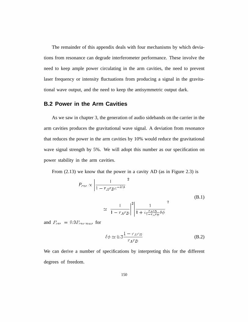
The remainderof this appendixdealswith four mechanismsby which devia-
tions from resonancecandegradeinterferometerperformance.Theseinvolve the
needto keep ample power circulating in the arm cavities, the needto prevent
laser frequencyor intensity fluctuationsfrom producinga signal in the gravita-
tional waveoutput,and the needto keepthe antisymmetricoutputdark.
B.2 Power in the Arm Cavities
As we sawin chapter3, thegenerationof audiosidebandson thecarrierin the
arm cavitiesproducesthe gravitationalwavesignal. A deviationfrom resonance
that reducesthepowerin thearmcavitiesby 10%would reducethegravitational
wave signal strengthby 5%. We will adoptthis numberas our specification on
power stability in the arm cavities.
From (2.13) we know that the power in a cavity AD (as in Figure2.3) is
������� �� � �� ���������
�
�� � ���
� ���������� �"!# � � � � !
$&%� (B.1)
and�����'�)(+*-,/.&�����'�10���2
for
$&% *-,/31� � �4���� � (B.2)
We can derive a numberof specificationsby interpretingthis for the different
degreesof freedom.
150
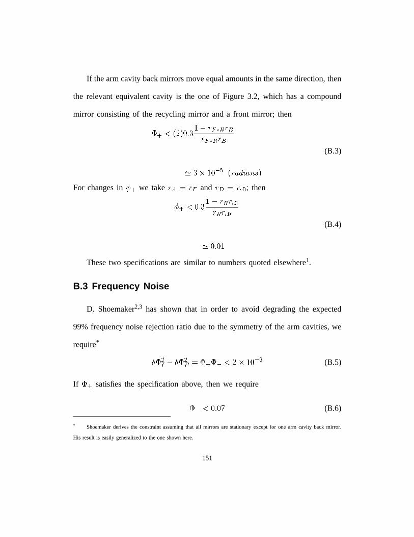
If thearmcavity backmirrorsmoveequalamountsin thesamedirection,then
the relevantequivalentcavity is the one of Figure 3.2, which hasa compound
mirror consistingof the recyclingmirror anda front mirror; then
������������ ���� ����������������������
� � �! #"$� ��%!&(')%!*�+ (B.3)
For changesin , � we take ��-/.0��� and ��12.0��3)4 ; then
, � �5�� 6�7� ������384� � ��384
�� 6� �(B.4)
Thesetwo specificationsaresimilar to numbersquotedelsewhere1.
B.3 Frequency Noise
D. Shoemaker2,3 has shown that in order to avoid degradingthe expected
99% frequencynoiserejectionratio dueto the symmetryof the arm cavities,we
require*
9 �;:< 9 ��:= . � � � �/� � � #> (B.5)
If� �
satisfiesthe specificationabove,then we require
� �5�? ��A@(B.6)
* Shoemakerderivesthe constraintassumingthat all mirrors are stationaryexceptfor one arm cavity back mirror.
His result is easilygeneralizedto the oneshownhere.
151
B.4 Intensity Noise
Since the gravitational wave signal is proportional to the product of the
laserpower and���
, low frequencydeviationsin the latter can couple in-band
fluctuationsin the former into the gravitational wave output. If 100 mW of
laserpoweris pickedoff for the purposeof powerstabilization,thenthe relative
intensity noise(just after the pick-off, assumingthat it is limited by shot noise
in the referencephotodetector)will be
������� �� ������� �������� ���
(B.7)
Now if thepick-off is locatedbetweenthemode-cleaner(seefootnoteon p.8)and
the recyclingmirror, thenthe low-passnatureof the recyclingcavity will reduce
this noiseat the beamsplitter by abouta factor of 50 ( "!� #!$! ):
�%���&�'(�� �*)+�-, ����/.0. � ���
(B.8)
If our target interferometersensitivity is 1 ��� �(24365� ���
, correspondingto
� ��7(8 �9� ���� .:2 � ���
, then we require
���<; 1 ����=2
(B.9)
B.5 Dark at the Antisymmetric Output
If the light returning from the two arm cavitiesdoesnot interfereperfectly
destructivelyat the antisymmetricoutput, then the additionalphotonshitting the
152
photodetectortherewill generateexcessshotnoise. It is believedthat about1%
of the power returningto the beamsplitter will arrive at the antisymmetricport
photodiodebecauseof mirror-imperfection-induceddifferencesin beamshapeor
intensity. We adoptthe requirementthat no morethanan additional0.1%of the
powerreturningto thebeamsplitterexit theantisymmetricport dueto deviations
in���
and � � .
For � �����, ���� ���� � ���������� ���� , so we require
����� ���� ! �#"$�%�'&
(B.10)
and†
��� !)( &*� � �(B.11)
To derivethespecificationfor � � , wenotethatthephaseof thelight returning
to thebeamsplitter changes+-,��/.0 �213�4 0� 3�4 &*5%�
timesfasterfor � � thanfor���
,
so that the specificationmust be tighter by this factor:
� � !76 &�� �98(B.12)
B.6 Summary
For our final set of specifications,we choosethe tightestconstrainton each
of the degreesof freedom:
† Specifyingseparatelimits on : � and ; � , in order to ensuredarknessat the antisymmetricport, is a conservative
strategysince the power leaving the antisymmetricport is actually proportionalto : �=<?> 1@BADC ; � . A slightly more
sophisticatednumericalservomodelthanthe onein Chapter6 would showthat the effect of residualdeviationsin : � is
partially cancelledby opposingdeviationsproducedin ; � by the loop feedingbackto ; � .
153
������� ��� �(B.13)
� �����������(B.14)
� ��� �� ��(B.15)
� ��� ������(B.16)
We demand that the RMS deviations in any of these degrees of freedom not
exceed the above-listed bounds.
154

155
Cited References
1 Technical Supplement to the LIGO Construction Proposal, internal LIGO doc-
ument, (1993), p. B-3.
2 D. Shoemaker, LIGO Working Paper #109, Internal LIGO document, (1991).
3 D. Shoemaker, Modulation and topology: Deviations from resonance, Internal
LIGO document, (1991).
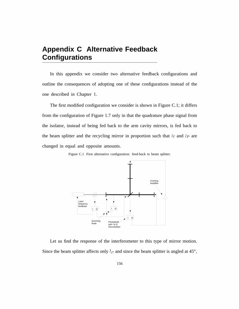
Appendix C Alternative FeedbackConfigurations
In this appendixwe considertwo alternativefeedbackconfigurationsand
outline the consequencesof adoptingone of theseconfigurationsinsteadof the
one describedin Chapter1.
Thefirst modifiedconfigurationwe consideris shownin FigureC.1; it differs
from theconfigurationof Figure1.7 only in that thequadraturephasesignalfrom
the isolator, insteadof being fed back to the arm cavity mirrors, is fed back to
the beamsplitter and the recycling mirror in proportionsuchthat���
and���
are
changedin equaland oppositeamounts.
Figure C.1 First alternativeconfiguration: feed-backto beamsplitter.
I Q
I Q
I Q
Photodiode with I & Q Demodulator
Laserfrequencyfeedback
Summing Node
Inverting Amplifier
Let us find the responseof the interferometerto this type of mirror motion.
Sincethebeamsplitteraffectsonly���
andsincethebeamsplitter is angledat 45� ,
156
this occurswhen the beamsplitter is displacedby�
as much as the recycling
mirror ( �������� �� ���� �� ) and we let
��� ��� ���� �� ������� (C.1)
representthis combinationof displacements.To derivethe transferfunction from
� �to ��� we first note that motion of the recycling mirror producesno signal
here, and we chooseto use that combinationof beam splitter and recycling
mirror motion which makesthe audio sidebandspropagatingtowards the two
input mirrors exactly equalin amplitudeandoppositein phase.This occursfor
��� � ������ � ��� ��� . Then theseaudio sidebandswill interfere destructivelyon
the symmetricside of the beamsplitter and constructivelyon the antisymmetric
side, so that
"!$#&%(' )+* -,/.103254 �76 � (C.2)
"!$#8%(' � "%9';:5#=<?> � �=@��ACB�DFEE A�G. DFEE A(C.3)
This result hasno importanteffects on systemperformancesincewe still have
"! # % ' !$#�H�'.
Next we note that
!=I7%9' � !=I$J�' � !=I=J�'K<�>(C.4)
since,as before,the characteristicfrequenciesexperiencedby the sidebandsare
all very high.
157
Finally we look at the responsein ��� and ��� . The abovecombinationof dis-
placements,with����� ��� �� � ������ , mustproducea frequency-independentsignal
in ��� and ��� becausetheaudiosidebandspresentat theseopticaloutputshavenot
interactedwith the arm cavities.Let us find the differencebetweenthis displace-
ment and ��� . We want to considerthe beamsplitter and recycling mirror as a
compoundmirror which is a sourceof audiosidebands,andwe want to solvefor
theproportionof displacementfor which thesidebandsgeneratedin thedirection
of the perpendiculararm are exactly equaland oppositethosegeneratedin the
directionof thein-line arm. Motion of thebeamsplitteraloneproducessidebands
propagatingtowardsbotharms,in theamount � ���� �������! #"�$ � �&%('*) $ � � � � ����+ ,in thedirectionof theperpendiculararmandin theamount� � � �-����� "�$ � �.)�� � ��� + ,in thedirectionof the in-line arm. Therecyclingmirror whendisplacedproduces
sidebandsof the samesize � � �0/ ) $ � � �� (if we take � � )�� ) propagatingtowards
both arms. Setting the total sidebandspropagatingtowardsthe two armsequal
and opposite,and neglectingbeamsplitter loss, we get:
� � 21, 1 ' 1� � �4365 "�$
� �7� + ,(C.5)
for the ratio of displacementswhich producesa frequency-independentresponse
in ��� and ��� . Since
8:9&;6<-=�>@? 8:9-AB<-=�>C? ED(C.6)
158
we must have
����������� �������������� � ��������� �������������
�� �� �!��������� � �����������"� #%$�# $� # $�
&' ()(�+*-, �.�
(C.7)
and
� �0/1�!� � �� � � ��� � � � � �0/1�����"� # �# � # �
&' (2(�3*4, �.� (C.8)
Theseeffectscanbe summarizedby writing the new plant56
as follows
567698 : �<;=�>�!�
: � ;�/1�!�: :: :
56�? (C.9)
where56�?
differs from6�?
only in its upperright element.The analysisand
designmethodspresentedin Chapter6 still apply. The non-zeroelementsin the
upperright sub-blockrepresentadditionalnoisesummedinto the common-mode
subsystemfrom the differential subsystem.Thesewill degradethe performance
of the system. In a numericalanalysisusing the samecontrollersas in Table
6.6, the predictedperformanceis the sameas in that example,except that in
the @ 8 loop the RMS residualdeviationis increasedto � ACB � :?ED
. A word of
cautionis appropriatehere.The specsderivedin AppendixB implicitly assumed
very-low-frequencydeviationsfrom resonanceandtheirgeneralizationto dynamic
deviations is not obvious. Moreover, becauseof the method used to assess
performancenumerically,we implicitly changedthedynamicgeneralizationof the
performancespecificationswhenwe switchedplants,andthis is partly responsible
159
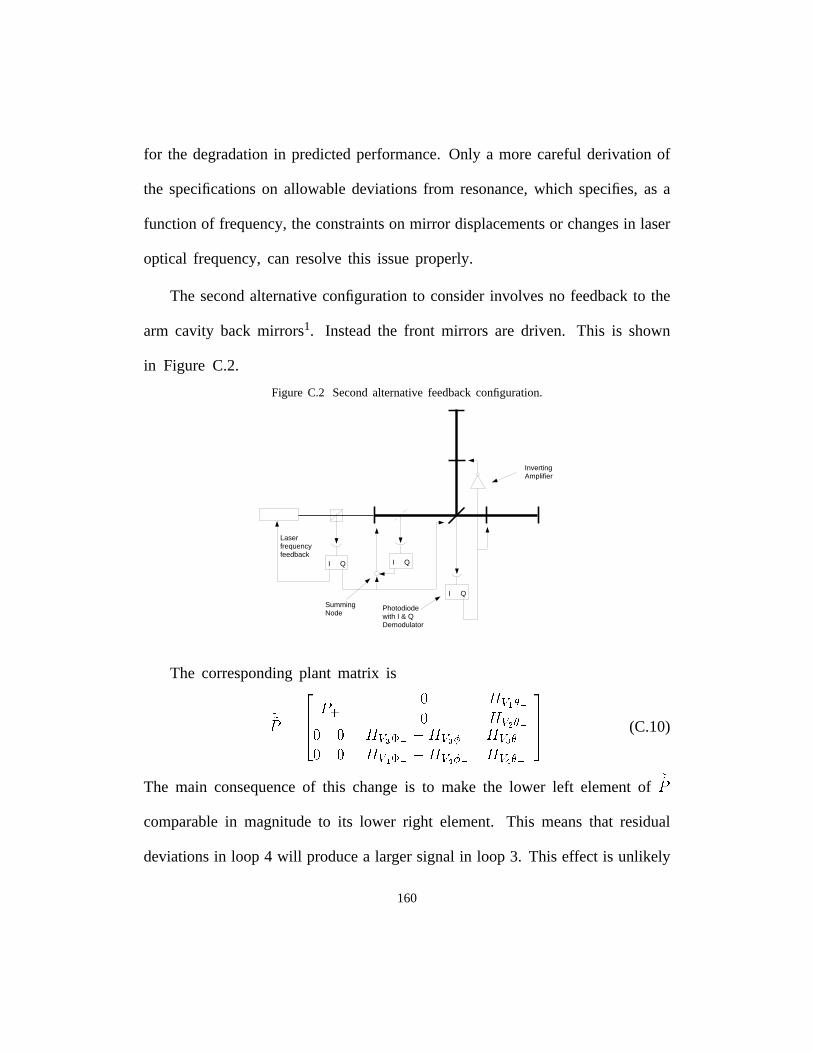
for the degradationin predictedperformance.Only a morecarefulderivationof
the specificationson allowabledeviationsfrom resonance,which specifies,as a
functionof frequency,theconstraintson mirror displacementsor changesin laser
optical frequency,can resolvethis issueproperly.
The secondalternativeconfigurationto considerinvolvesno feedbackto the
arm cavity back mirrors1. Insteadthe front mirrors are driven. This is shown
in Figure C.2.
Figure C.2 Secondalternativefeedbackconfiguration.
I Q
I Q
I Q
Photodiode with I & Q Demodulator
Laserfrequencyfeedback
Summing Node
Inverting Amplifier
The correspondingplant matrix is
� ������� � ��� ���
� ������ �� �� �
� ����� � ������ � ������ �� ��� � � � � � � � � � � � �
(C.10)
The main consequenceof this changeis to make the lower left elementof� ��
comparablein magnitudeto its lower right element. This meansthat residual
deviationsin loop 4 will producea largersignalin loop 3. This effect is unlikely
160
to be importantsincethe specificationsare tighter for deviationsin loop 4 than
in loop 3.
One additional considerationin analyzing thesealternativesis that in the
presenceof mixer phaseerror, the commonmode and differential subsystems
becomefully coupled.They canno longerbe analyzed(asin FigureD.1) astwo
subsystemswhich are independentexceptthat one injects noise into the other,
since signalsnow flow in both directions. Both performanceand stability can
be affected.
161

162
Cited References
1 L. Sievers, private communication, (1993).
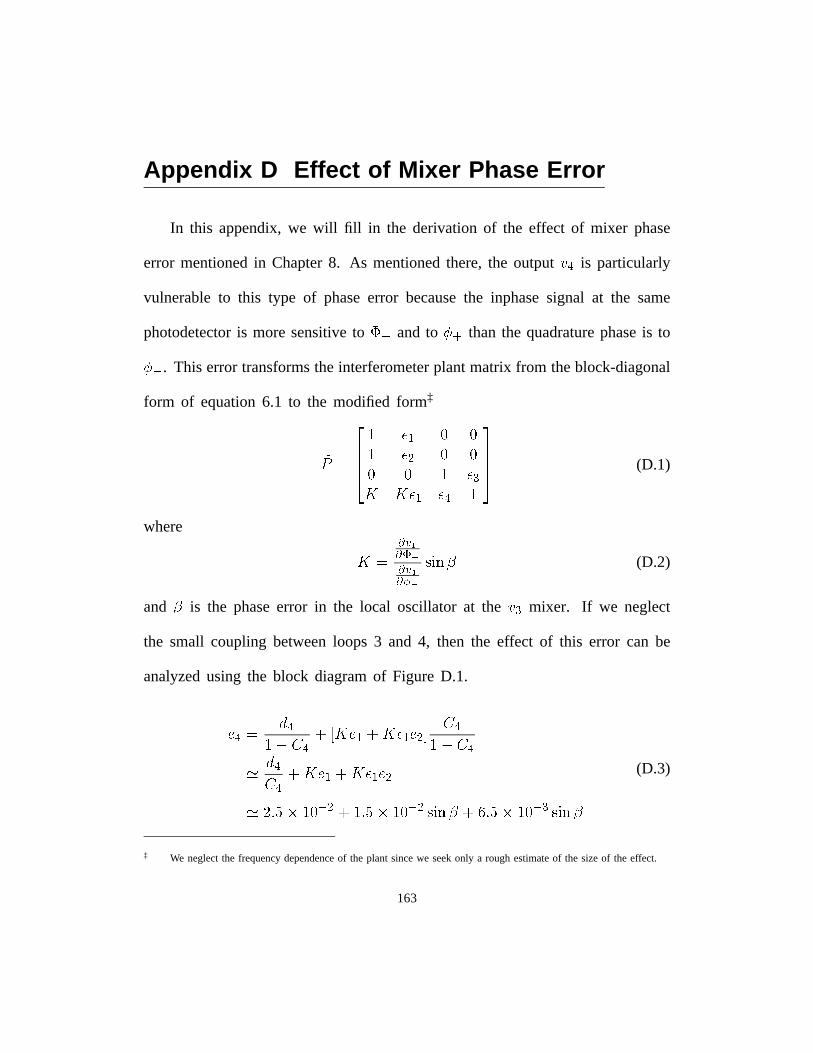
Appendix D Effect of Mixer Phase Error
In this appendix,we will fill in the derivationof the effect of mixer phase
error mentionedin Chapter8. As mentionedthere,the output ��� is particularly
vulnerableto this type of phaseerror becausethe inphasesignal at the same
photodetectoris moresensitiveto���
andto � � than the quadraturephaseis to
��� . This error transformstheinterferometerplantmatrix from theblock-diagonal
form of equation6.1 to the modified form‡
�� ��� � � ��� � �� � ���� � ��� � � (D.1)
where
��� ��������! ���#"��$�%'&(*)�+
(D.2)
and+
is the phaseerror in the local oscillator at the � � mixer. If we neglect
the small coupling betweenloops 3 and 4, then the effect of this error can be
analyzedusing the block diagramof Figure D.1.
,�� � - � . �0/21 � , � / � ��� , ��3 . � . �- �. �0/ � , � / � ��� , �46587 �� � � / 9587 :� � � &
(;)<+ />= 587 :� � � &(;)<+
(D.3)
‡ We neglectthe frequencydependenceof the plant sincewe seekonly a roughestimateof the sizeof the effect.
163
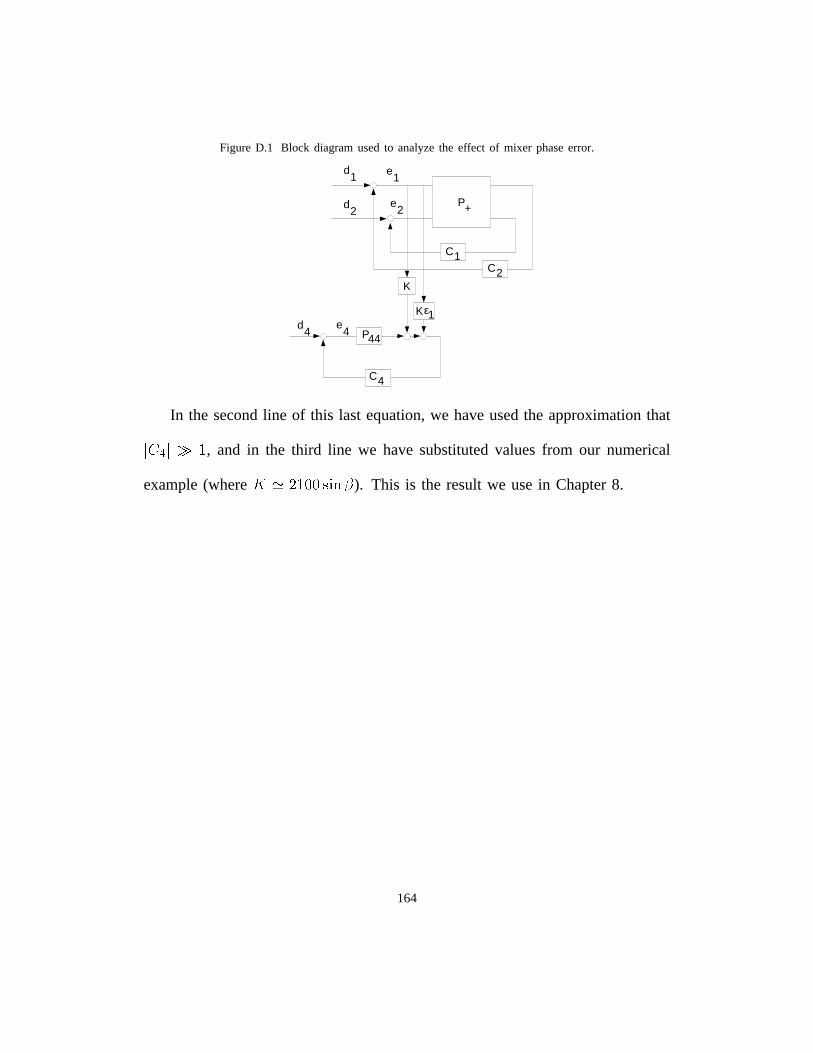
Figure D.1 Block diagram used to analyze the effect of mixer phase error.
P+
P44
d1
C4
d2
d4
e1
e2
e4
K
ε1K
C1C2
In the second line of this last equation, we have used the approximation that
��� �, and in the third line we have substituted values from our numerical
example (where � � �������� �� ). This is the result we use in Chapter 8.
164