thermohaline ocean circulation - harvard university€¦ · s. rahmstorf: thermohaline ocean...

S. Rahmstorf: Thermohaline Ocean Circulation. In: Encyclopedia of Quaternary Sciences, Edited by S. A. Elias. Elsevier, Amsterdam 2006.

1

Thermohaline Ocean Circulation

Stefan Rahmstorf

The thermohaline circulation is that part of the ocean circulation which is driven by fluxes of heat and freshwater across the sea surface and subsequent interior mixing of heat and salt. The term thus refers to a driving mechanism. Important features of the thermohaline circulation are deep water formation, spreading of deep waters partly through deep boundary currents, upwelling and near-surface currents, together leading to a large-scale deep overturning motion of the oceans. The large heat transport of the thermohaline circulation makes it important for climate, and its non-linear and potentially abrupt response to forcing have been invoked to explain abrupt glacial climate changes. Anthropogenic climate change is likely to weaken the thermohaline circulation in future, with some risk of triggering abrupt and/or irreversible changes.

“It appears to be extremely difficult, if not quite impossible, to account for this degree of cold at the bottom of the sea in the torrid zone, on any other supposition than that of cold currents from the poles; and the utility of these currents in tempering the excessive heats of these climates is too evident to require any illustration”

Sir Benjamin Thompson, 1797

What is the thermohaline circulation? In 1751 the captain of an English slave-

trading ship made the first recorded measurement of deep ocean temperatures – he discovered that the water a mile below his ship was very cold, despite the subtropical location. In 1797 another Englishman, Benjamin Thompson, correctly explained this discovery by cold currents from the poles, as part of what later became known as the thermohaline circulation.

As opposed to wind-driven currents and tides (the latter are due to the gravity of moon and sun), the thermohaline circulation (often abbreviated as THC) is that part of the ocean circulation which is driven by fluxes of heat and freshwater across the sea surface and subsequent interior mixing of heat and salt - hence the name thermo-haline. (Geothermal heat sources at the ocean bottom play a minor role.) The term thermohaline circulation thus refers to a particular driving mechanism; it is a physical, not an observational concept.

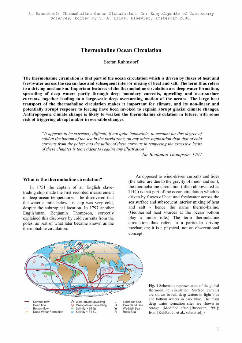
Fig. 1 Schematic representation of the global thermohaline circulation. Surface currents are shown in red, deep waters in light blue and bottom waters in dark blue. The main deep water formation sites are shown in orange. (Modified after [Broecker, 1991]; from [Kuhlbrodt, et al., submitted].)


2

The distinction of thermohaline versus wind-driven circulation originates in a 19th-Century dispute on whether ocean currents are primarily due to the wind pushing along the water or whether they are “convection currents” due to heating and cooling, or evaporation and precipitation. In 1908 Johan Sandström performed a series of classic tank experiments at Bornö oceanographic station in Sweden to investigate both possibilities [Sandström, 1908], describing the properties of “wind-driven circulation” and “thermal circulation”. To include salinity, the latter was later extended to “thermohaline circulation”, a term which by the 1920s appeared in the classic oceanography textbook by Albert Defant [Defant, 1929]. The ocean’s density distribution, which determines pressure gradients and thus circulation, is itself affected by currents and mixing. Thermohaline and wind-driven currents therefore interact in non-linear ways and cannot be separated by oceanographic measurements. There are thus two distinct physical forcing mechanisms, but not two uniquely separable circulations. Changing the wind stress will alter the thermohaline circulation; altering thermohaline forcing will also change the wind-driven currents.

A related, complementary concept is that of meridional overturning circulation (MOC). This refers to the north-south flow as a function of latitude and depth, often integrated in east-west direction across an ocean basin or the globe and graphically depicted as a stream function. The streamlines typically show a large-scale slow overturning motion of the ocean. The MOC can be easily diagnosed from a model, and in principle it can be measured in the ocean.

Although the terms THC and MOC are often inaccurately used as if synonymous, there strictly is no one-to-one relation between the two. The MOC includes clearly wind-driven parts, namely the Ekman cells consisting of the transport in the near-surface Ekman layer and a return flow below it. And a direct contribution of wind-driven currents even to the large-scale, deeper overturning is being increasingly discussed. On the other hand, the THC is of course not confined to the meridional direction; rather, it is also associated with zonal overturning cells. Hence, care should be taken with the terminology: the term THC should be reserved for a particular forcing mechanism, e.g., when discussing the influence of cooling or freshwater forcing on the ocean circulation. The term MOC should be used

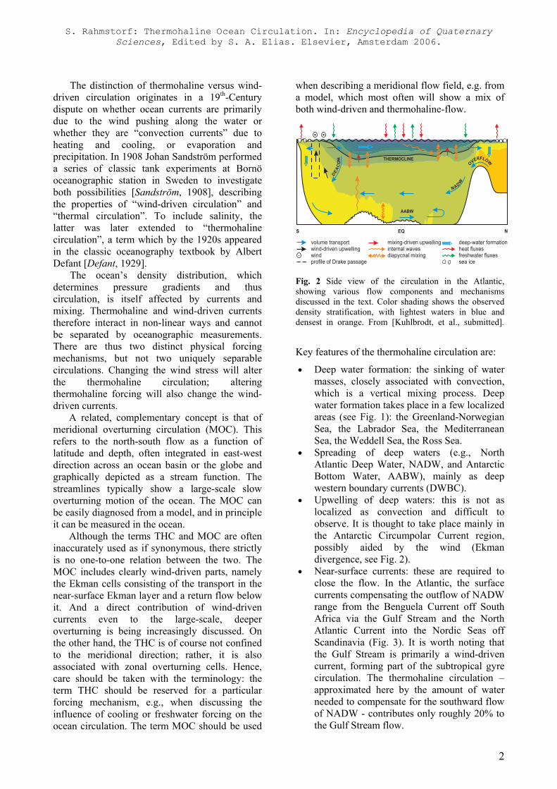
when describing a meridional flow field, e.g. from a model, which most often will show a mix of both wind-driven and thermohaline-flow.

Fig. 2 Side view of the circulation in the Atlantic, showing various flow components and mechanisms discussed in the text. Color shading shows the observed density stratification, with lightest waters in blue and densest in orange. From [Kuhlbrodt, et al., submitted].

Key features of the thermohaline circulation are:

• Deep water formation: the sinking of water masses, closely associated with convection, which is a vertical mixing process. Deep water formation takes place in a few localized areas (see Fig. 1): the Greenland-Norwegian Sea, the Labrador Sea, the Mediterranean Sea, the Weddell Sea, the Ross Sea.

• Spreading of deep waters (e.g., North Atlantic Deep Water, NADW, and Antarctic Bottom Water, AABW), mainly as deep western boundary currents (DWBC).

• Upwelling of deep waters: this is not as localized as convection and difficult to observe. It is thought to take place mainly in the Antarctic Circumpolar Current region, possibly aided by the wind (Ekman divergence, see Fig. 2).

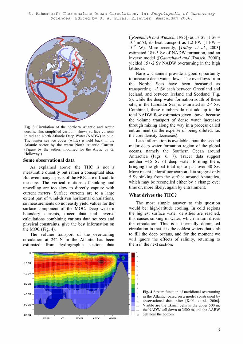
• Near-surface currents: these are required to close the flow. In the Atlantic, the surface currents compensating the outflow of NADW range from the Benguela Current off South Africa via the Gulf Stream and the North Atlantic Current into the Nordic Seas off Scandinavia (Fig. 3). It is worth noting that the Gulf Stream is primarily a wind-driven current, forming part of the subtropical gyre circulation. The thermohaline circulation – approximated here by the amount of water needed to compensate for the southward flow of NADW - contributes only roughly 20% to the Gulf Stream flow.


3

Fig. 3 Circulation of the northern Atlantic and Arctic oceans. This simplified cartoon shows surface currents in red and North Atlantic Deep Water (NADW) in blue. The winter sea ice cover (white) is held back in the Atlantic sector by the warm North Atlantic Current. (Figure by the author, modified for the Arctic by G. Holloway.)

Some observational data As explained above, the THC is not a

measurable quantity but rather a conceptual idea. But even many aspects of the MOC are difficult to measure. The vertical motions of sinking and upwelling are too slow to directly capture with current meters. Surface currents are to a large extent part of wind-driven horizontal circulations, so measurements do not easily yield values for the surface component of the MOC. Deep western boundary currents, tracer data and inverse calculations combining various data sources and physical constraints, give the best information on the MOC (Fig. 4).

The volume transport of the overturning circulation at 24º N in the Atlantic has been estimated from hydrographic section data

([Roemmich and Wunsch, 1985]) as 17 Sv (1 Sv = 106 m3/s), its heat transport as 1.2 PW (1 PW = 1015 W). More recently, [Talley, et al., 2003] estimated 18+-5 Sv of NADW formation, and an inverse model ([Ganachaud and Wunsch, 2000]) yielded 15+-2 Sv NADW overturning in the high latitudes.

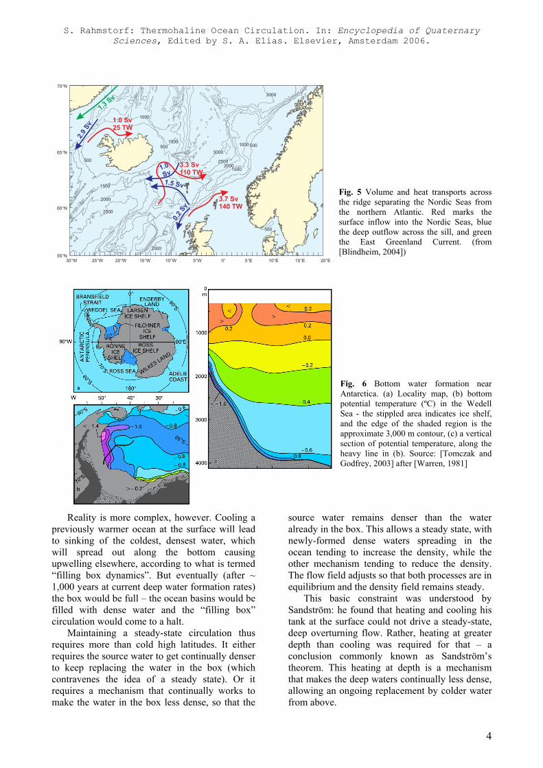
Narrow channels provide a good opportunity to measure deep water flows. The overflows from the Nordic Seas have been measured as transporting ~3 Sv each between Greenland and Iceland, and between Iceland and Scotland (Fig. 5), while the deep water formation south of these sills, in the Labrador Sea, is estimated as 2-4 Sv. Combined, these numbers do not add up to the total NADW flow estimates given above, because the volume transport of dense water increases through mixing along the way in a process called entrainment (at the expense of being diluted, i.e. the core density decreases).

Less information is available about the second major deep water formation region of the global oceans, namely the Southern Ocean around Antarctica (Figs. 6, 7). Tracer data suggest another ~15 Sv of deep water forming there, bringing the global total up to just over 30 Sv. More recent chlorofluorocarbon data suggest only 5 Sv sinking from the surface around Antarctica, which may be reconciled either by a change over time or, more likely, again by entrainment.

What drives the THC? The most simple answer to this question

would be: high-latitude cooling. In cold regions the highest surface water densities are reached, this causes sinking of water, which in turn drives the circulation. This is a thermally dominated circulation in that it is the coldest waters that sink to fill the deep oceans, and for the moment we will ignore the effects of salinity, returning to them in the next section.

Fig. 4 Stream function of meridional overturning in the Atlantic, based on a model constrained by observational data, after [Köhl, et al., 2006]. Visible are the Ekman cells in the upper 500 m, the NADW cell down to 3500 m, and the AABW cell near the bottom.


4

Fig. 5 Volume and heat transports across the ridge separating the Nordic Seas from the northern Atlantic. Red marks the surface inflow into the Nordic Seas, blue the deep outflow across the sill, and green the East Greenland Current. (from [Blindheim, 2004])

Fig. 6 Bottom water formation near Antarctica. (a) Locality map, (b) bottom potential temperature (ºC) in the Wedell Sea - the stippled area indicates ice shelf, and the edge of the shaded region is the approximate 3,000 m contour, (c) a vertical section of potential temperature, along the heavy line in (b). Source: [Tomczak and Godfrey, 2003] after [Warren, 1981]

Reality is more complex, however. Cooling a previously warmer ocean at the surface will lead to sinking of the coldest, densest water, which will spread out along the bottom causing upwelling elsewhere, according to what is termed “filling box dynamics”. But eventually (after ~ 1,000 years at current deep water formation rates) the box would be full – the ocean basins would be filled with dense water and the “filling box” circulation would come to a halt.

Maintaining a steady-state circulation thus requires more than cold high latitudes. It either requires the source water to get continually denser to keep replacing the water in the box (which contravenes the idea of a steady state). Or it requires a mechanism that continually works to make the water in the box less dense, so that the

source water remains denser than the water already in the box. This allows a steady state, with newly-formed dense waters spreading in the ocean tending to increase the density, while the other mechanism tending to reduce the density. The flow field adjusts so that both processes are in equilibrium and the density field remains steady.

This basic constraint was understood by Sandström: he found that heating and cooling his tank at the surface could not drive a steady-state, deep overturning flow. Rather, heating at greater depth than cooling was required for that – a conclusion commonly known as Sandström’s theorem. This heating at depth is a mechanism that makes the deep waters continually less dense, allowing an ongoing replacement by colder water from above.


5

What is this mechanism in the real ocean, where heating occurs at (or very near) the surface due to the sun? As Sandström already speculated, it is the downward penetration of heat by mixing. The result is the classic advection-diffusion balance: in steady state, at any given point in the depths of the oceans, the slow diffusion of heat by turbulent mixing is balanced by the equally slow transport of cold waters from the poles.

Downward mixing of heat requires energy to overcome frictional dissipation and to raise the potential energy stored in the water column, as heat penetrating downwards expands the deep water and lifts up the waters above. This is the energy supply of the thermohaline circulation: in an energetic sense, it is driven by turbulent mixing in the ocean’s interior. This is why mixing appears in the definition of thermohaline circulation given at the outset of this article (quoted from [Rahmstorf, 2002]).

The power supply of the turbulence which causes this mixing is both by tidal motions and by the winds. The energy supply needed for generating the observed global overturning motion of ~30 Sv can be estimated from the advection-diffusion balance and the observed density field as ~0.4 TW ([Munk and Wunsch, 1998]). This can be compared with the power input by winds and tides, estimated as roughly 1 TW each, although these estimates are rather uncertain. With a mixing efficiency of 20%, 0.4 TW would be available for driving the thermohaline circulation (the remaining 80% are dissipated).

Although the energy supply of the thermohaline circulation thus ultimately comes from winds and tides, it is useful to keep the established term “thermohaline circulation” (as we keep calling “steam engine” a machine that is powered by coal or wood), in order to distinguish

this driving mechanism from a completely different kind: the direct generation of large-scale currents by the frictional action of wind on the water surface. Apart from obviously driving surface currents, this mechanism could also be involved in driving the deep-reaching MOC, in a manner proposed by [Toggweiler and Samuels, 1995].

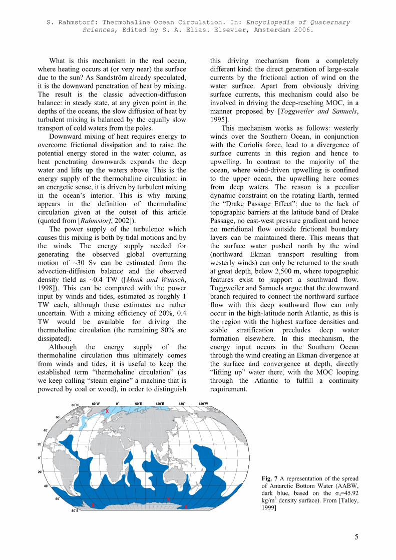
This mechanism works as follows: westerly winds over the Southern Ocean, in conjunction with the Coriolis force, lead to a divergence of surface currents in this region and hence to upwelling. In contrast to the majority of the ocean, where wind-driven upwelling is confined to the upper ocean, the upwelling here comes from deep waters. The reason is a peculiar dynamic constraint on the rotating Earth, termed the “Drake Passage Effect”: due to the lack of topographic barriers at the latitude band of Drake Passage, no east-west pressure gradient and hence no meridional flow outside frictional boundary layers can be maintained there. This means that the surface water pushed north by the wind (northward Ekman transport resulting from westerly winds) can only be returned to the south at great depth, below 2,500 m, where topographic features exist to support a southward flow. Toggweiler and Samuels argue that the downward branch required to connect the northward surface flow with this deep southward flow can only occur in the high-latitude north Atlantic, as this is the region with the highest surface densities and stable stratification precludes deep water formation elsewhere. In this mechanism, the energy input occurs in the Southern Ocean through the wind creating an Ekman divergence at the surface and convergence at depth, directly “lifting up” water there, with the MOC looping through the Atlantic to fulfill a continuity requirement.

Fig. 7 A representation of the spread of Antarctic Bottom Water (AABW, dark blue, based on the σ4=45.92 kg/m3 density surface). From [Talley, 1999]

80˚S

80˚N

60˚W 0˚ 60˚E 120˚E 180˚ 120˚W

60˚

40˚

20˚

0˚

20˚

40˚

60˚

XX

X

X80˚N

80˚S

XX

X

X


6

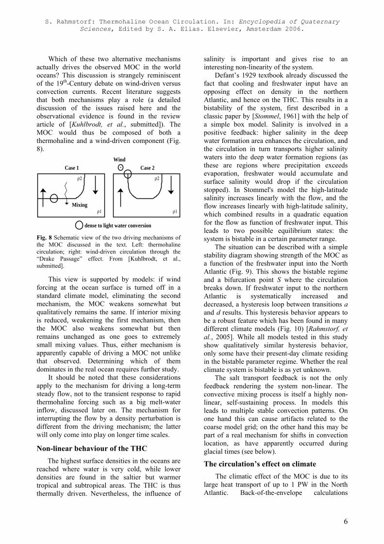
Which of these two alternative mechanisms actually drives the observed MOC in the world oceans? This discussion is strangely reminiscent of the 19th-Century debate on wind-driven versus convection currents. Recent literature suggests that both mechanisms play a role (a detailed discussion of the issues raised here and the observational evidence is found in the review article of [Kuhlbrodt, et al., submitted]). The MOC would thus be composed of both a thermohaline and a wind-driven component (Fig. 8).

Fig. 8 Schematic view of the two driving mechanisms of the MOC discussed in the text. Left: thermohaline circulation; right: wind-driven circulation through the “Drake Passage” effect. From [Kuhlbrodt, et al., submitted].

This view is supported by models: if wind forcing at the ocean surface is turned off in a standard climate model, eliminating the second mechanism, the MOC weakens somewhat but qualitatively remains the same. If interior mixing is reduced, weakening the first mechanism, then the MOC also weakens somewhat but then remains unchanged as one goes to extremely small mixing values. Thus, either mechanism is apparently capable of driving a MOC not unlike that observed. Determining which of them dominates in the real ocean requires further study. It should be noted that these considerations apply to the mechanism for driving a long-term steady flow, not to the transient response to rapid thermohaline forcing such as a big melt-water inflow, discussed later on. The mechanism for interrupting the flow by a density perturbation is different from the driving mechanism; the latter will only come into play on longer time scales.

Non-linear behaviour of the THC The highest surface densities in the oceans are

reached where water is very cold, while lower densities are found in the saltier but warmer tropical and subtropical areas. The THC is thus thermally driven. Nevertheless, the influence of

salinity is important and gives rise to an interesting non-linearity of the system.

Defant’s 1929 textbook already discussed the fact that cooling and freshwater input have an opposing effect on density in the northern Atlantic, and hence on the THC. This results in a bistability of the system, first described in a classic paper by [Stommel, 1961] with the help of a simple box model. Salinity is involved in a positive feedback: higher salinity in the deep water formation area enhances the circulation, and the circulation in turn transports higher salinity waters into the deep water formation regions (as these are regions where precipitation exceeds evaporation, freshwater would accumulate and surface salinity would drop if the circulation stopped). In Stommel's model the high-latitude salinity increases linearly with the flow, and the flow increases linearly with high-latitude salinity, which combined results in a quadratic equation for the flow as function of freshwater input. This leads to two possible equilibrium states: the system is bistable in a certain parameter range.

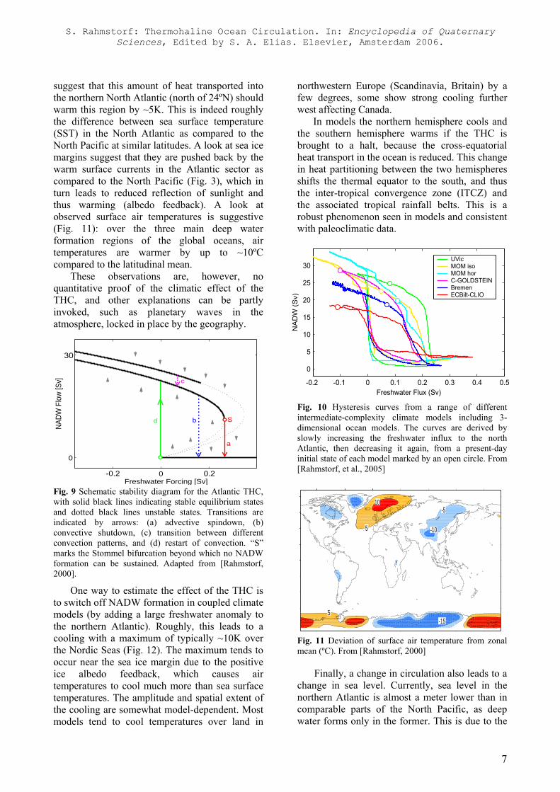
The situation can be described with a simple stability diagram showing strength of the MOC as a function of the freshwater input into the North Atlantic (Fig. 9). This shows the bistable regime and a bifurcation point S where the circulation breaks down. If freshwater input to the northern Atlantic is systematically increased and decreased, a hysteresis loop between transitions a and d results. This hysteresis behavior appears to be a robust feature which has been found in many different climate models (Fig. 10) [Rahmstorf, et al., 2005]. While all models tested in this study show qualitatively similar hysteresis behavior, only some have their present-day climate residing in the bistable parameter regime. Whether the real climate system is bistable is as yet unknown.

The salt transport feedback is not the only feedback rendering the system non-linear. The convective mixing process is itself a highly non-linear, self-sustaining process. In models this leads to multiple stable convection patterns. On one hand this can cause artifacts related to the coarse model grid; on the other hand this may be part of a real mechanism for shifts in convection location, as have apparently occurred during glacial times (see below).

The circulation’s effect on climate The climatic effect of the MOC is due to its large heat transport of up to 1 PW in the North Atlantic. Back-of-the-envelope calculations

Case 1

dense to light water conversion

Mixing

WindCase 2

ρ1 ρ1

ρ2 ρ2


7

suggest that this amount of heat transported into the northern North Atlantic (north of 24ºN) should warm this region by ~5K. This is indeed roughly the difference between sea surface temperature (SST) in the North Atlantic as compared to the North Pacific at similar latitudes. A look at sea ice margins suggest that they are pushed back by the warm surface currents in the Atlantic sector as compared to the North Pacific (Fig. 3), which in turn leads to reduced reflection of sunlight and thus warming (albedo feedback). A look at observed surface air temperatures is suggestive (Fig. 11): over the three main deep water formation regions of the global oceans, air temperatures are warmer by up to ~10ºC compared to the latitudinal mean.

These observations are, however, no quantitative proof of the climatic effect of the THC, and other explanations can be partly invoked, such as planetary waves in the atmosphere, locked in place by the geography.

Fig. 9 Schematic stability diagram for the Atlantic THC, with solid black lines indicating stable equilibrium states and dotted black lines unstable states. Transitions are indicated by arrows: (a) advective spindown, (b) convective shutdown, (c) transition between different convection patterns, and (d) restart of convection. “S” marks the Stommel bifurcation beyond which no NADW formation can be sustained. Adapted from [Rahmstorf, 2000].

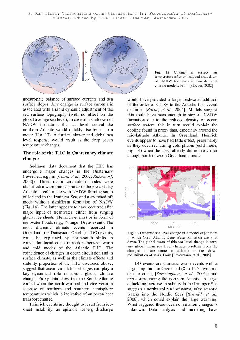
One way to estimate the effect of the THC is to switch off NADW formation in coupled climate models (by adding a large freshwater anomaly to the northern Atlantic). Roughly, this leads to a cooling with a maximum of typically ~10K over the Nordic Seas (Fig. 12). The maximum tends to occur near the sea ice margin due to the positive ice albedo feedback, which causes air temperatures to cool much more than sea surface temperatures. The amplitude and spatial extent of the cooling are somewhat model-dependent. Most models tend to cool temperatures over land in

northwestern Europe (Scandinavia, Britain) by a few degrees, some show strong cooling further west affecting Canada.

In models the northern hemisphere cools and the southern hemisphere warms if the THC is brought to a halt, because the cross-equatorial heat transport in the ocean is reduced. This change in heat partitioning between the two hemispheres shifts the thermal equator to the south, and thus the inter-tropical convergence zone (ITCZ) and the associated tropical rainfall belts. This is a robust phenomenon seen in models and consistent with paleoclimatic data.

Fig. 10 Hysteresis curves from a range of different intermediate-complexity climate models including 3-dimensional ocean models. The curves are derived by slowly increasing the freshwater influx to the north Atlantic, then decreasing it again, from a present-day initial state of each model marked by an open circle. From [Rahmstorf, et al., 2005]

Fig. 11 Deviation of surface air temperature from zonal mean (ºC). From [Rahmstorf, 2000]

Finally, a change in circulation also leads to a change in sea level. Currently, sea level in the northern Atlantic is almost a meter lower than in comparable parts of the North Pacific, as deep water forms only in the former. This is due to the

−0.1 0 0.1

0

20

Freshwater Forcing [Sv]

NA

DW

Flo

w [S

v]

oS

30

a

b

c

d S

-0.2 0.2

-0.2 -0.1 0 0.1 0.2 0.3 0.4 0.5

0

5

10

15

20

25

30

Freshwater Flux (Sv)

NA

DW

(S

v)

UVicMOM isoMOM horC-GOLDSTEINBremenECBilt-CLIO

-155

10

5

-5

-10


8

geostrophic balance of surface currents and sea surface slopes. Any change in surface currents is associated with a rapid dynamic adjustment of the sea surface topography (with no effect on the global average sea level); in case of a shutdown of NADW formation, the sea level around the northern Atlantic would quickly rise by up to a meter (Fig. 13). A further, slower and global sea level response would result as the deep ocean temperature changes.

The role of the THC in Quaternary climate changes

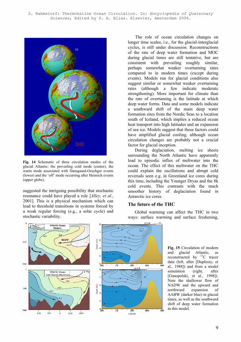
Sediment data document that the THC has undergone major changes in the Quaternary (reviewed, e.g., in [Clark, et al., 2002; Rahmstorf, 2002]). Three major circulation modes were identified: a warm mode similar to the present-day Atlantic, a cold mode with NADW forming south of Iceland in the Irminger Sea, and a switched-off mode without significant formation of NADW (Fig. 14). The latter appears to have occurred after major input of freshwater, either from surging glacial ice sheets (Heinrich events) or in form of meltwater floods (e.g., Younger Dryas event). The most dramatic climate events recorded in Greenland, the Dansgaard-Oeschger (DO) events, could be explained by north-south shifts in convection location, i.e. transitions between warm and cold modes of the Atlantic THC. The coincidence of changes in ocean circulation and in surface climate, as well as the climate effects and stability properties of the THC discussed above, suggest that ocean circulation changes can play a key dynamical role in abrupt glacial climate change. Proxy data show that the South Atlantic cooled when the north warmed and vice versa, a see-saw of northern and southern hemisphere temperatures which is indicative of an ocean heat transport change.

Heinrich events are thought to result from ice-sheet instability: an episodic iceberg discharge

Fig. 12 Change in surface air temperature after an induced shut-down of NADW formation in two different climate models. From [Stocker, 2002]

would have provided a large freshwater addition of the order of 0.1 Sv to the Atlantic for several centuries [Roche, et al., 2004]. Models suggest this could have been enough to stop all NADW formation due to the reduced density of ocean surface waters; this in turn would explain the cooling found in proxy data, especially around the mid-latitude Atlantic. In Greenland, Heinrich events appear to have had little effect, presumably as they occurred during cold phases (cold mode, Fig. 14) when the THC already did not reach far enough north to warm Greenland climate.

Fig. 13 Dynamic sea level change in a model experiment in which North Atlantic Deep Water formation was shut down. The global mean of this sea level change is zero; any global mean sea level changes resulting from the changed climate come in addition to the shown redistribution of mass. From [Levermann, et al., 2005]

DO events are dramatic warm events with a large amplitude in Greenland (8 to 16 ºC within a decade or so, [Severinghaus, et al., 2003]) and areas surrounding the northern Atlantic. A large coinciding increase in salinity in the Irminger Sea suggests a northward push of warm, salty Atlantic waters into the Nordic Seas [Kreveld, et al., 2000], which could explain the large warming. What triggered these ocean circulation changes is unknown. Data analysis and modeling have


9

Fig. 14 Schematic of three circulation modes of the glacial Atlantic: the prevailing cold mode (center), the warm mode associated with Dansgaard-Oeschger events (lower) and the ‘off’ mode occurring after Heinrich events (upper globe).

suggested the intriguing possibility that stochastic resonance could have played a role [Alley, et al., 2001]. This is a physical mechanism which can lead to threshold transitions in systems forced by a weak regular forcing (e.g., a solar cycle) and stochastic variability.

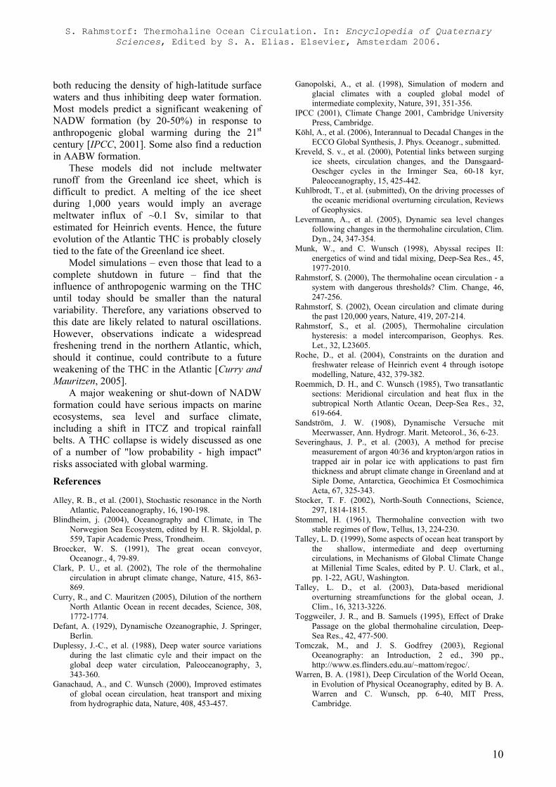
The role of ocean circulation changes on longer time scales, i.e., for the glacial-interglacial cycles, is still under discussion. Reconstructions of the rate of deep water formation and MOC during glacial times are still tentative, but are consistent with prevailing roughly similar, perhaps somewhat weaker overturning rates compared to in modern times (except during events). Models run for glacial conditions also suggest similar or somewhat weaker overturning rates (although a few indicate moderate strengthening). More important for climate than the rate of overturning is the latitude at which deep water forms. Data and some models indicate a southward shift of the main deep water formation sites from the Nordic Seas to a location south of Iceland, which implies a reduced ocean heat transport into high latitudes and an expansion of sea ice. Models suggest that these factors could have amplified glacial cooling, although ocean circulation changes are probably not a crucial factor for glacial inception.

During deglaciation, melting ice sheets surrounding the North Atlantic have apparently lead to episodic influx of meltwater into the ocean. The effect of this meltwater on the THC could explain the oscillations and abrupt cold reversals seen e.g. in Greenland ice cores during this time, including the Younger Dryas and the 8k cold events. This contrasts with the much smoother history of deglaciation found in Antarctic ice cores.

The future of the THC Global warming can affect the THC in two

ways: surface warming and surface freshening,

Fig. 15 Circulation of modern and glacial Atlantic, as reconstructed by 13C tracer data (left, after [Duplessy, et al., 1988]) and from a model simulation (right, after [Ganopolski, et al., 1998]). Note the shallower flow of NADW and the upward and northward expansion of AABW (darker blue) in glacial times, as well as the southward shift of deep water formation in this model.


10

both reducing the density of high-latitude surface waters and thus inhibiting deep water formation. Most models predict a significant weakening of NADW formation (by 20-50%) in response to anthropogenic global warming during the 21st century [IPCC, 2001]. Some also find a reduction in AABW formation.

These models did not include meltwater runoff from the Greenland ice sheet, which is difficult to predict. A melting of the ice sheet during 1,000 years would imply an average meltwater influx of ~0.1 Sv, similar to that estimated for Heinrich events. Hence, the future evolution of the Atlantic THC is probably closely tied to the fate of the Greenland ice sheet.

Model simulations – even those that lead to a complete shutdown in future – find that the influence of anthropogenic warming on the THC until today should be smaller than the natural variability. Therefore, any variations observed to this date are likely related to natural oscillations. However, observations indicate a widespread freshening trend in the northern Atlantic, which, should it continue, could contribute to a future weakening of the THC in the Atlantic [Curry and Mauritzen, 2005].

A major weakening or shut-down of NADW formation could have serious impacts on marine ecosystems, sea level and surface climate, including a shift in ITCZ and tropical rainfall belts. A THC collapse is widely discussed as one of a number of "low probability - high impact" risks associated with global warming.

References

Alley, R. B., et al. (2001), Stochastic resonance in the North Atlantic, Paleoceanography, 16, 190-198.

Blindheim, j. (2004), Oceanography and Climate, in The Norwegion Sea Ecosystem, edited by H. R. Skjoldal, p. 559, Tapir Academic Press, Trondheim.

Broecker, W. S. (1991), The great ocean conveyor, Oceanogr., 4, 79-89.

Clark, P. U., et al. (2002), The role of the thermohaline circulation in abrupt climate change, Nature, 415, 863-869.

Curry, R., and C. Mauritzen (2005), Dilution of the northern North Atlantic Ocean in recent decades, Science, 308, 1772-1774.

Defant, A. (1929), Dynamische Ozeanographie, J. Springer, Berlin.

Duplessy, J.-C., et al. (1988), Deep water source variations during the last climatic cyle and their impact on the global deep water circulation, Paleoceanography, 3, 343-360.

Ganachaud, A., and C. Wunsch (2000), Improved estimates of global ocean circulation, heat transport and mixing from hydrographic data, Nature, 408, 453-457.

Ganopolski, A., et al. (1998), Simulation of modern and glacial climates with a coupled global model of intermediate complexity, Nature, 391, 351-356.

IPCC (2001), Climate Change 2001, Cambridge University Press, Cambridge.

Köhl, A., et al. (2006), Interannual to Decadal Changes in the ECCO Global Synthesis, J. Phys. Oceanogr., submitted.

Kreveld, S. v., et al. (2000), Potential links between surging ice sheets, circulation changes, and the Dansgaard-Oeschger cycles in the Irminger Sea, 60-18 kyr, Paleoceanography, 15, 425-442.

Kuhlbrodt, T., et al. (submitted), On the driving processes of the oceanic meridional overturning circulation, Reviews of Geophysics.

Levermann, A., et al. (2005), Dynamic sea level changes following changes in the thermohaline circulation, Clim. Dyn., 24, 347-354.

Munk, W., and C. Wunsch (1998), Abyssal recipes II: energetics of wind and tidal mixing, Deep-Sea Res., 45, 1977-2010.

Rahmstorf, S. (2000), The thermohaline ocean circulation - a system with dangerous thresholds? Clim. Change, 46, 247-256.

Rahmstorf, S. (2002), Ocean circulation and climate during the past 120,000 years, Nature, 419, 207-214.

Rahmstorf, S., et al. (2005), Thermohaline circulation hysteresis: a model intercomparison, Geophys. Res. Let., 32, L23605.

Roche, D., et al. (2004), Constraints on the duration and freshwater release of Heinrich event 4 through isotope modelling, Nature, 432, 379-382.

Roemmich, D. H., and C. Wunsch (1985), Two transatlantic sections: Meridional circulation and heat flux in the subtropical North Atlantic Ocean, Deep-Sea Res., 32, 619-664.

Sandström, J. W. (1908), Dynamische Versuche mit Meerwasser, Ann. Hydrogr. Marit. Meteorol., 36, 6-23.

Severinghaus, J. P., et al. (2003), A method for precise measurement of argon 40/36 and krypton/argon ratios in trapped air in polar ice with applications to past firn thickness and abrupt climate change in Greenland and at Siple Dome, Antarctica, Geochimica Et Cosmochimica Acta, 67, 325-343.

Stocker, T. F. (2002), North-South Connections, Science, 297, 1814-1815.

Stommel, H. (1961), Thermohaline convection with two stable regimes of flow, Tellus, 13, 224-230.

Talley, L. D. (1999), Some aspects of ocean heat transport by the shallow, intermediate and deep overturning circulations, in Mechanisms of Global Climate Change at Millenial Time Scales, edited by P. U. Clark, et al., pp. 1-22, AGU, Washington.

Talley, L. D., et al. (2003), Data-based meridional overturning streamfunctions for the global ocean, J. Clim., 16, 3213-3226.

Toggweiler, J. R., and B. Samuels (1995), Effect of Drake Passage on the global thermohaline circulation, Deep-Sea Res., 42, 477-500.

Tomczak, M., and J. S. Godfrey (2003), Regional Oceanography: an Introduction, 2 ed., 390 pp., http://www.es.flinders.edu.au/~mattom/regoc/.

Warren, B. A. (1981), Deep Circulation of the World Ocean, in Evolution of Physical Oceanography, edited by B. A. Warren and C. Wunsch, pp. 6-40, MIT Press, Cambridge.

thermohaline ocean circulation - harvard university€¦ · s. rahmstorf: thermohaline ocean...

Documents