Thermoacoustic Devices

Peter in ’t panhuisSjoerd Rienstra

Han Slot

9th May 2007

Introduction Outline Modeling Linear Theory Streaming Conclusions Future Work Further reading

Introduction

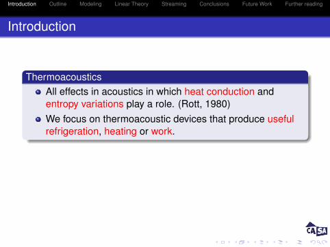
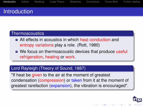
ThermoacousticsAll effects in acoustics in which heat conduction andentropy variations play a role. (Rott, 1980)We focus on thermoacoustic devices that produce usefulrefrigeration, heating or work.

Lord Rayleigh (Theory of Sound, 1887)

"If heat be given to the air at the moment of greatestcondensation (compression) or taken from it at the moment ofgreatest rarefaction (expansion), the vibration is encouraged".

Introduction Outline Modeling Linear Theory Streaming Conclusions Future Work Further reading

Introduction

ThermoacousticsAll effects in acoustics in which heat conduction andentropy variations play a role. (Rott, 1980)We focus on thermoacoustic devices that produce usefulrefrigeration, heating or work.

Lord Rayleigh (Theory of Sound, 1887)

"If heat be given to the air at the moment of greatestcondensation (compression) or taken from it at the moment ofgreatest rarefaction (expansion), the vibration is encouraged".

Introduction Outline Modeling Linear Theory Streaming Conclusions Future Work Further reading

Outline

1 Modeling

2 Linear Theory

3 Streaming

4 Conclusions

5 Future Work

Introduction Outline Modeling Linear Theory Streaming Conclusions Future Work Further reading

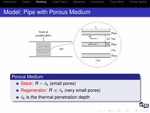
Model: Pipe with Porous Medium

Porous MediumStack: R ∼ δk (small pores)Regenerator: R � δk (very small pores)δk is the thermal penetration depth

Introduction Outline Modeling Linear Theory Streaming Conclusions Future Work Further reading

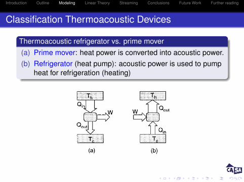
Classification Thermoacoustic Devices

Thermoacoustic refrigerator vs. prime mover

(a) Prime mover: heat power is converted into acoustic power.(b) Refrigerator (heat pump): acoustic power is used to pump

heat for refrigeration (heating)

Introduction Outline Modeling Linear Theory Streaming Conclusions Future Work Further reading

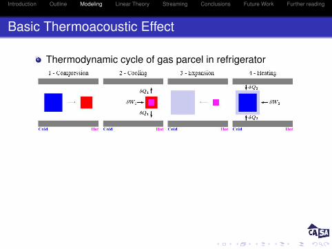
Basic Thermoacoustic Effect

Thermodynamic cycle of gas parcel in refrigerator

Bucket brigade: heat is shuttled along the stack

Introduction Outline Modeling Linear Theory Streaming Conclusions Future Work Further reading

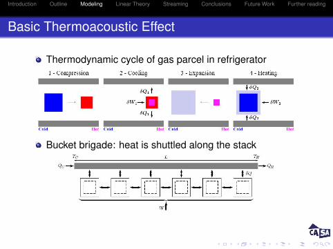
Basic Thermoacoustic Effect

Thermodynamic cycle of gas parcel in refrigerator

Bucket brigade: heat is shuttled along the stack

Introduction Outline Modeling Linear Theory Streaming Conclusions Future Work Further reading

Linear Theory

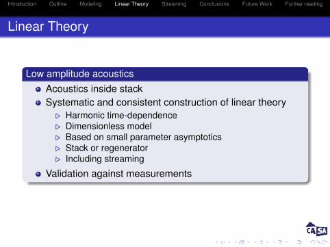
Low amplitude acousticsAcoustics inside stackSystematic and consistent construction of linear theory

. Harmonic time-dependence

. Dimensionless model

. Based on small parameter asymptotics

. Stack or regenerator

. Including streaming

Validation against measurements

Introduction Outline Modeling Linear Theory Streaming Conclusions Future Work Further reading

Linearization

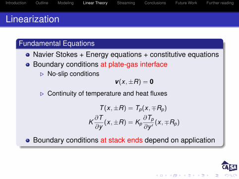
Fundamental EquationsNavier Stokes + Energy equations + constitutive equationsBoundary conditions at plate-gas interface

. No-slip conditionsv(x ,±R) = 0

. Continuity of temperature and heat fluxes

T (x ,±R) = Tp(x ,∓Rp)

K∂T∂y

(x ,±R) = Kp∂Tp

∂y ′ (x ,∓Rp)

Boundary conditions at stack ends depend on application

Introduction Outline Modeling Linear Theory Streaming Conclusions Future Work Further reading

Dimensionless Model

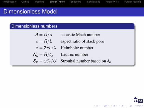
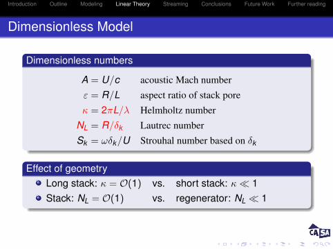
Dimensionless numbers

A = U/c acoustic Mach number

ε = R/L aspect ratio of stack pore

κ = 2πL/λ Helmholtz number

NL = R/δk Lautrec number

Sk = ωδk/U Strouhal number based on δk

Introduction Outline Modeling Linear Theory Streaming Conclusions Future Work Further reading

Dimensionless Model

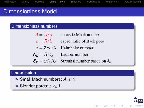
Dimensionless numbers

A = U/c acoustic Mach number

ε = R/L aspect ratio of stack pore

κ = 2πL/λ Helmholtz number

NL = R/δk Lautrec number

Sk = ωδk/U Strouhal number based on δk

LinearizationSmall Mach numbers: A � 1Slender pores: ε � 1

Introduction Outline Modeling Linear Theory Streaming Conclusions Future Work Further reading

Dimensionless Model

Dimensionless numbers

A = U/c acoustic Mach number

ε = R/L aspect ratio of stack pore

κ = 2πL/λ Helmholtz number

NL = R/δk Lautrec number

Sk = ωδk/U Strouhal number based on δk

Effect of geometryLong stack: κ = O(1) vs. short stack: κ � 1Stack: NL = O(1) vs. regenerator: NL � 1

Introduction Outline Modeling Linear Theory Streaming Conclusions Future Work Further reading

Dimensionless Model

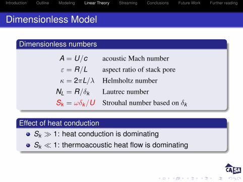
Dimensionless numbers

A = U/c acoustic Mach number

ε = R/L aspect ratio of stack pore

κ = 2πL/λ Helmholtz number

NL = R/δk Lautrec number

Sk = ωδk/U Strouhal number based on δk

Effect of heat conductionSk � 1: heat conduction is dominatingSk � 1: thermoacoustic heat flow is dominating

Introduction Outline Modeling Linear Theory Streaming Conclusions Future Work Further reading

Linearization

Neglect second order terms

Expand in powers of A:

f (x , y , t) = f0(x , y) + ARe[f1(x , y)eit] +O(A2), A � 1

No mean velocity: u0 = 0. Constant mean pressure p0

We are interested in T0, p1 and u1

We use the method of slow variation. Slender pore assumption: ε � 1. p1 and T0 do not depend on y. Define U1 =

∫ 10 u1dy

. System ODE’s for T0, p1 and U1

Introduction Outline Modeling Linear Theory Streaming Conclusions Future Work Further reading

Linearization

Neglect second order terms

Expand in powers of A:

f (x , y , t) = f0(x , y) + ARe[f1(x , y)eit] +O(A2), A � 1

No mean velocity: u0 = 0. Constant mean pressure p0

We are interested in T0, p1 and u1

We use the method of slow variation. Slender pore assumption: ε � 1. p1 and T0 do not depend on y. Define U1 =

∫ 10 u1dy

. System ODE’s for T0, p1 and U1

Introduction Outline Modeling Linear Theory Streaming Conclusions Future Work Further reading

Linearization

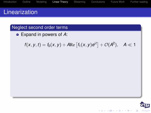
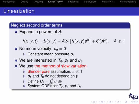
Neglect second order terms

Expand in powers of A:

f (x , y , t) = f0(x , y) + ARe[f1(x , y)eit] +O(A2), A � 1

No mean velocity: u0 = 0. Constant mean pressure p0

We are interested in T0, p1 and u1

We use the method of slow variation. Slender pore assumption: ε � 1. p1 and T0 do not depend on y. Define U1 =

∫ 10 u1dy

. System ODE’s for T0, p1 and U1

Introduction Outline Modeling Linear Theory Streaming Conclusions Future Work Further reading

Linearization

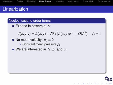
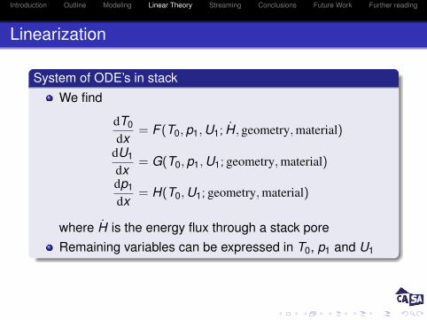
System of ODE’s in stackWe find

dT0

dx= F (T0, p1, U1; H, geometry, material)

dU1

dx= G(T0, p1, U1; geometry, material)

dp1

dx= H(T0, U1; geometry, material)

where H is the energy flux through a stack poreRemaining variables can be expressed in T0, p1 and U1

Introduction Outline Modeling Linear Theory Streaming Conclusions Future Work Further reading

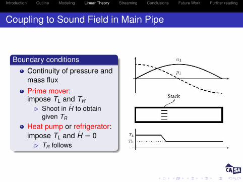
Coupling to Sound Field in Main Pipe

Boundary conditionsContinuity of pressure andmass fluxPrime mover:impose TL and TR

. Shoot in H to obtaingiven TR

Heat pump or refrigerator:impose TL and H = 0

. TR follows

Introduction Outline Modeling Linear Theory Streaming Conclusions Future Work Further reading

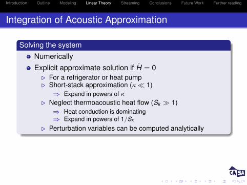
Integration of Acoustic Approximation

Solving the systemNumericallyExplicit approximate solution if H = 0

. For a refrigerator or heat pump

. Short-stack approximation (κ � 1)⇒ Expand in powers of κ

. Neglect thermoacoustic heat flow (Sk � 1)⇒ Heat conduction is dominating⇒ Expand in powers of 1/Sk

. Perturbation variables can be computed analytically

Introduction Outline Modeling Linear Theory Streaming Conclusions Future Work Further reading

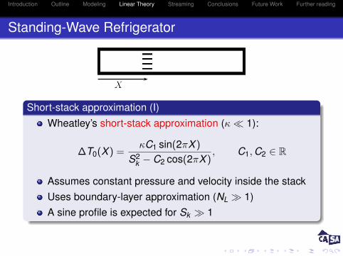
Standing-Wave Refrigerator

Short-stack approximation (I)Wheatley’s short-stack approximation (κ � 1):

∆T0(X ) =κC1 sin(2πX )

S2k − C2 cos(2πX )

, C1, C2 ∈ R

Assumes constant pressure and velocity inside the stackUses boundary-layer approximation (NL � 1)A sine profile is expected for Sk � 1

Introduction Outline Modeling Linear Theory Streaming Conclusions Future Work Further reading

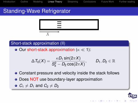
Standing-Wave Refrigerator

Short-stack approximation (II)Our short-stack approximation (κ � 1):

∆T0(X ) =κD1 sin(2πX )

S2k − D2 cos(2πX )

, D1, D2 ∈ R

Constant pressure and velocity inside the stack followsDoes NOT use boundary-layer approximationC1 6= D1 and C2 6= D2

Introduction Outline Modeling Linear Theory Streaming Conclusions Future Work Further reading

Standing-Wave Refrigerator

0.5 1 1.5 2 2.5 3 3.5 4 4.5−6

−4

−2

0

2

4

6

kX

tem

pera

ture

diff

eren

ce (

K)

numericsshort stackWheatley et al.measurements

0.5 1 1.5 2 2.5 3 3.5 4 4.5−0.25

−0.2

−0.15

−0.1

−0.05

0

0.05

0.1

0.15

0.2

0.25

kX

tem

pera

ture

diff

eren

ce (

K)

numericsshort stackWheatley et al.measurements

Sk = 1.0 Sk = 0.1

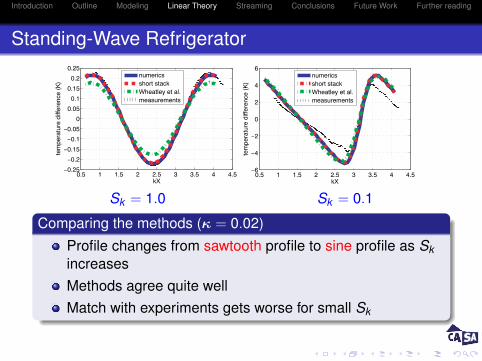
Comparing the methods (κ = 0.02)

Profile changes from sawtooth profile to sine profile as SkincreasesMethods agree quite wellMatch with experiments gets worse for small Sk

Introduction Outline Modeling Linear Theory Streaming Conclusions Future Work Further reading

Standing-Wave Refrigerator

0.5 1 1.5 2 2.5 3 3.5 4 4.5−6

−4

−2

0

2

4

6

kX

tem

pera

ture

diff

eren

ce (

K)

numericsshort stackWheatley et al.measurements

0.5 1 1.5 2 2.5 3 3.5 4 4.5−0.25

−0.2

−0.15

−0.1

−0.05

0

0.05

0.1

0.15

0.2

0.25

kX

tem

pera

ture

diff

eren

ce (

K)

numericsshort stackWheatley et al.measurements

Sk = 1.0 Sk = 0.1

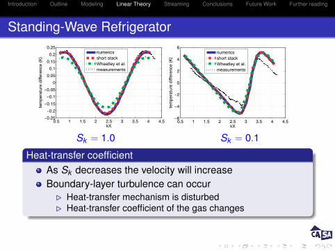
Heat-transfer coefficientAs Sk decreases the velocity will increaseBoundary-layer turbulence can occur

. Heat-transfer mechanism is disturbed

. Heat-transfer coefficient of the gas changes

Introduction Outline Modeling Linear Theory Streaming Conclusions Future Work Further reading

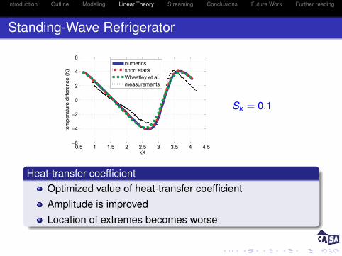
Standing-Wave Refrigerator

0.5 1 1.5 2 2.5 3 3.5 4 4.5−6

−4

−2

0

2

4

6

kX

tem

pera

ture

diff

eren

ce (

K)

numericsshort stackWheatley et al.measurements

Sk = 0.1

Heat-transfer coefficientOptimized value of heat-transfer coefficientAmplitude is improvedLocation of extremes becomes worse

Introduction Outline Modeling Linear Theory Streaming Conclusions Future Work Further reading

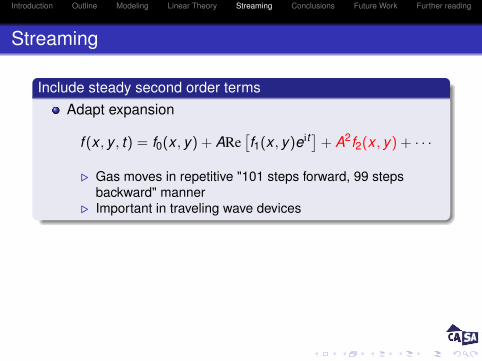
Streaming

Include steady second order termsAdapt expansion

f (x , y , t) = f0(x , y) + ARe[f1(x , y)eit] + A2f2(x , y) + · · ·

. Gas moves in repetitive "101 steps forward, 99 stepsbackward" manner

. Important in traveling wave devices

Time-averaged mass flux M

The time-averaged mass flux M is constantM = 0 in standing wave devices

Introduction Outline Modeling Linear Theory Streaming Conclusions Future Work Further reading

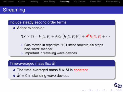
Streaming

Include steady second order termsAdapt expansion

f (x , y , t) = f0(x , y) + ARe[f1(x , y)eit] + A2f2(x , y) + · · ·

. Gas moves in repetitive "101 steps forward, 99 stepsbackward" manner

. Important in traveling wave devices

Time-averaged mass flux M

The time-averaged mass flux M is constantM = 0 in standing wave devices

Introduction Outline Modeling Linear Theory Streaming Conclusions Future Work Further reading

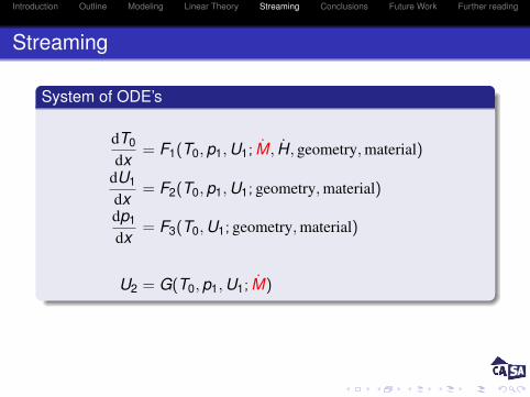
Streaming

System of ODE’s

dT0

dx= F1(T0, p1, U1; M, H, geometry, material)

dU1

dx= F2(T0, p1, U1; geometry, material)

dp1

dx= F3(T0, U1; geometry, material)

U2 = G(T0, p1, U1; M)

Introduction Outline Modeling Linear Theory Streaming Conclusions Future Work Further reading

Conclusions

ProgressLinear theory has been constructed

. Both for stacks and regenerators

. Including streamingLinear theory has been implemented numerically

. Applied to a standing wave refrigerator

. Good agreement with experiments

. Good agreement with analytic methods.We can compute:

. Temperature, pressure and velocity profiles in the stack

. Streaming terms in the stack

. Cooling and acoustic power

Introduction Outline Modeling Linear Theory Streaming Conclusions Future Work Further reading

Future work

OutlineImplement equations for a traveling wave device

. Streaming becomes importantStudy behavior of flow near stack ends

. Jet flow

. Vortex shedding

Include other non-linear effectsCheck validity for high amplitudes

Introduction Outline Modeling Linear Theory Streaming Conclusions Future Work Further reading

Further reading

N. RottThermoacousticsAdv. in Appl. Mech. (20), 1980.

G.W. SwiftThermoacoustic enginesJASA (84), 1988.

A.A. Atchley et al.Acoustically generated temperature gradients in short platesJASA (88), 1990.

J.C. Wheatley et al.An intrinsically irreversible thermoacoustic heat engineJASA (74), 1983.