Theory of Ordinal Utility/Indifference Curve Analysis:

Introduction: The indifference curve analysis approach was

first introduced by Slustsky, a Russian Economist in 1915. Later it was developed by J.R. Hicks and R.G.D. Allen in the year 1928.

In an article “ A Reconsideration of the theory of value”. And in his value and capital in 1939. It has been used to replace the neo-classical cardinal utility concept.

Introduction cont---- • These economist are the of view that it is wrong to

base the theory of consumption on two assumptions: • (i) That there is only one commodity which a person

will buy at one time. • (ii) The utility can be measured • Their point of view is that utility is purely subjective

and is immeasurable. Moreover an individual is interested in a combination of related goods and in the purchase of one commodity at one time. So they base the theory of consumption on the scale of preference and the ordinal ranks or orders his preferences

Meaning of indifference curve & definition

• The indifference curve indicates the various combinations of two goods which yield equal satisfaction to the consumer. By definition:

• "An indifference curve shows all the various combinations of two goods that give an equal amount of satisfaction to a consumer".

• An indifference curve is the locus of all commodity bundles (combinations) that give the consumer the same level of utility (ie, the consumer is indifferent between these bundles.

Indifference Schedule

Bundle/combination Quantity of

Peanut/X

Quantity of

Chocolate/Y

Utility

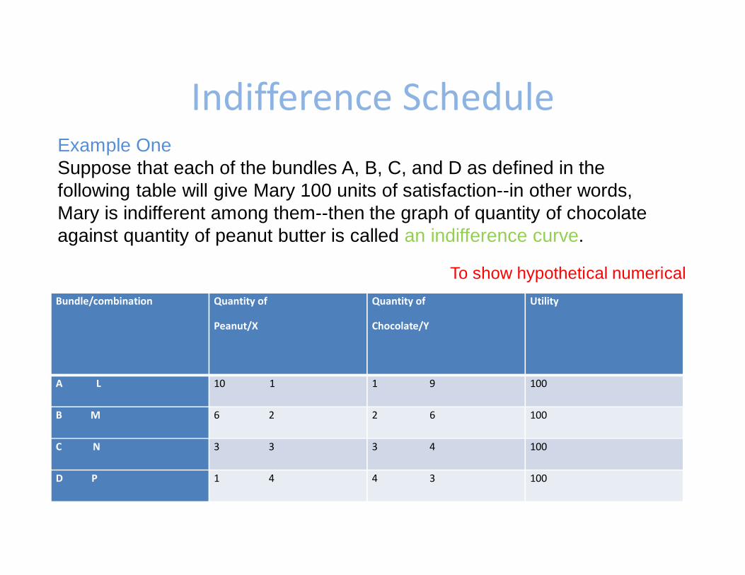
A L 10 1 1 9 100

B M 6 2 2 6 100

C N 3 3 3 4 100

D P 1 4 4 3 100

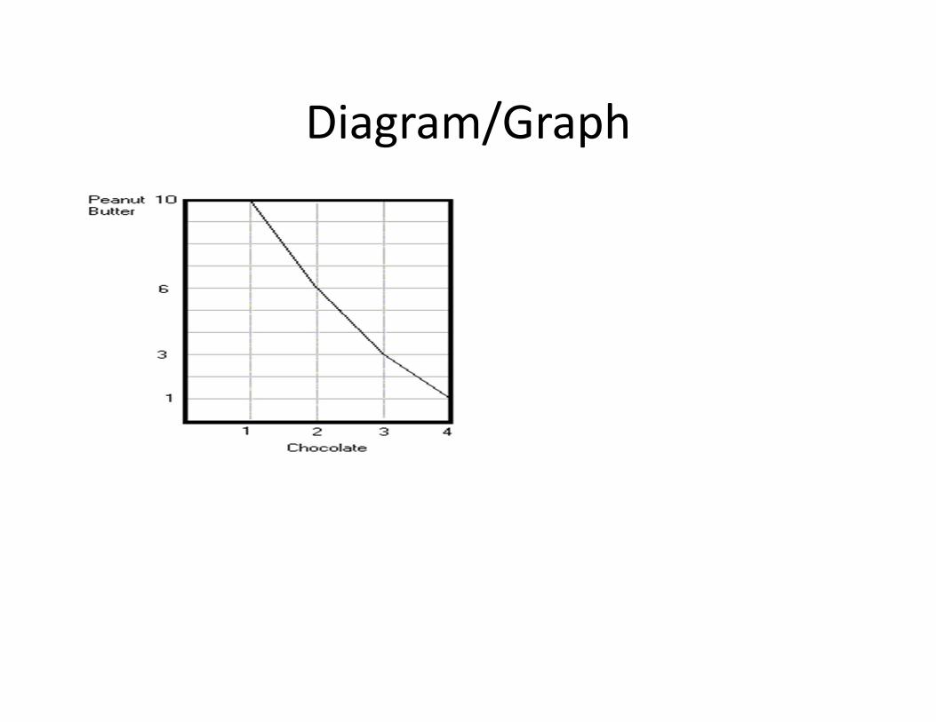
Example One Suppose that each of the bundles A, B, C, and D as defined in the following table will give Mary 100 units of satisfaction--in other words, Mary is indifferent among them--then the graph of quantity of chocolate against quantity of peanut butter is called an indifference curve.

To show hypothetical numerical

Indifference Schedule

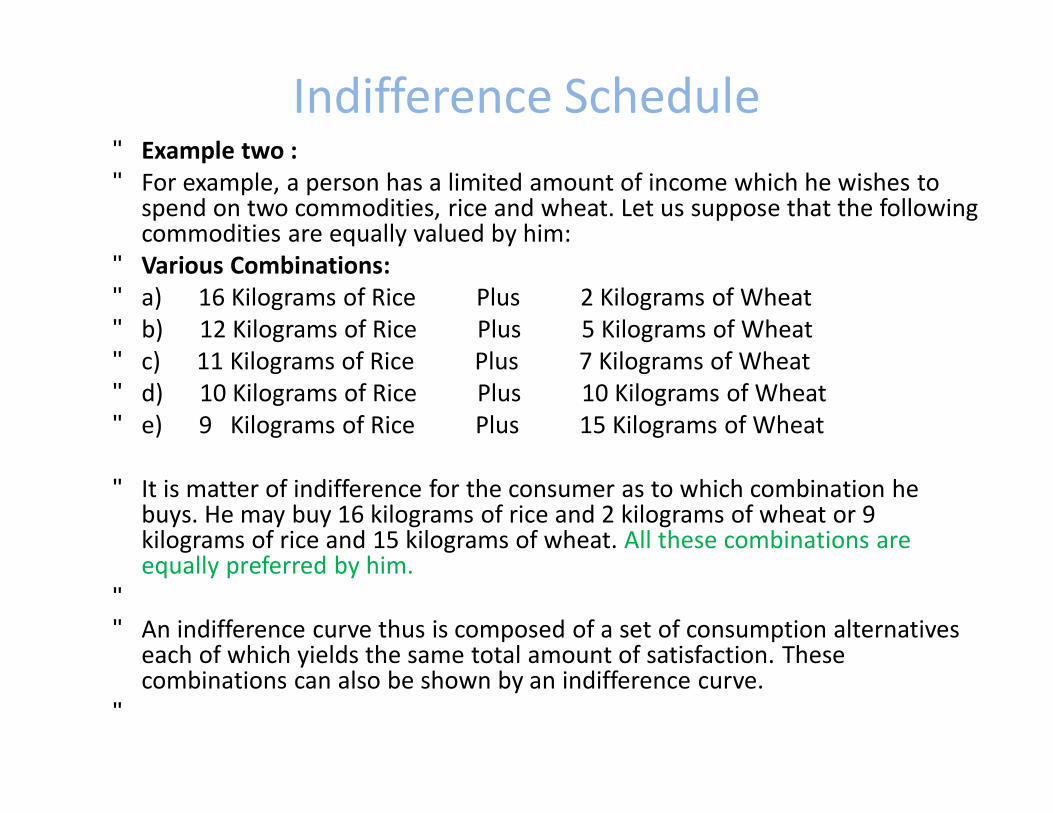
• Example two : • For example, a person has a limited amount of income which he wishes to

spend on two commodities, rice and wheat. Let us suppose that the following commodities are equally valued by him:

• Various Combinations: • a) 16 Kilograms of Rice Plus 2 Kilograms of Wheat • b) 12 Kilograms of Rice Plus 5 Kilograms of Wheat • c) 11 Kilograms of Rice Plus 7 Kilograms of Wheat • d) 10 Kilograms of Rice Plus 10 Kilograms of Wheat • e) 9 Kilograms of Rice Plus 15 Kilograms of Wheat

• It is matter of indifference for the consumer as to which combination he

buys. He may buy 16 kilograms of rice and 2 kilograms of wheat or 9 kilograms of rice and 15 kilograms of wheat. All these combinations are equally preferred by him.

• • An indifference curve thus is composed of a set of consumption alternatives

each of which yields the same total amount of satisfaction. These combinations can also be shown by an indifference curve.

•

Diagram/Graph

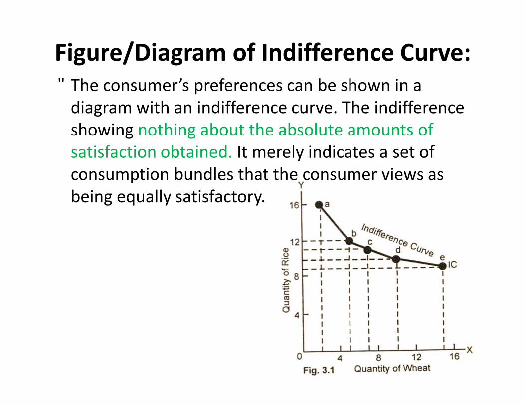
Figure/Diagram of Indifference Curve: • The consumer’s preferences can be shown in a

diagram with an indifference curve. The indifference showing nothing about the absolute amounts of satisfaction obtained. It merely indicates a set of consumption bundles that the consumer views as being equally satisfactory.

Cont-- • In fig. 1 we measure the quantity of wheat along X-axis (in kilograms)

and along Y-axis, the quantity of rice (in kilograms). IC is an indifference curve.

• It is shown in the diagram that a consumer may buy 12 kilograms of rice and 5 kilograms of wheat or 9 kilograms of rice and 15 kilogram of wheat. Both these combinations are equally preferred by him and he is indifferent to these two combinations. When the scale of preference of the consumer is graphed, by joining the points a, b, c, d, e, we obtain an Indifference Curve IC.

• • Every point on indifference curve represents a different combination

of the two goods and the consumer is indifferent between any two points on the indifference curve. All the combinations are equally desirable to the consumer. The consumer is indifferent as to which combination he receives. The Indifference Curve IC thus is a locus of different combinations of two goods which yield the same level of satisfaction.

•

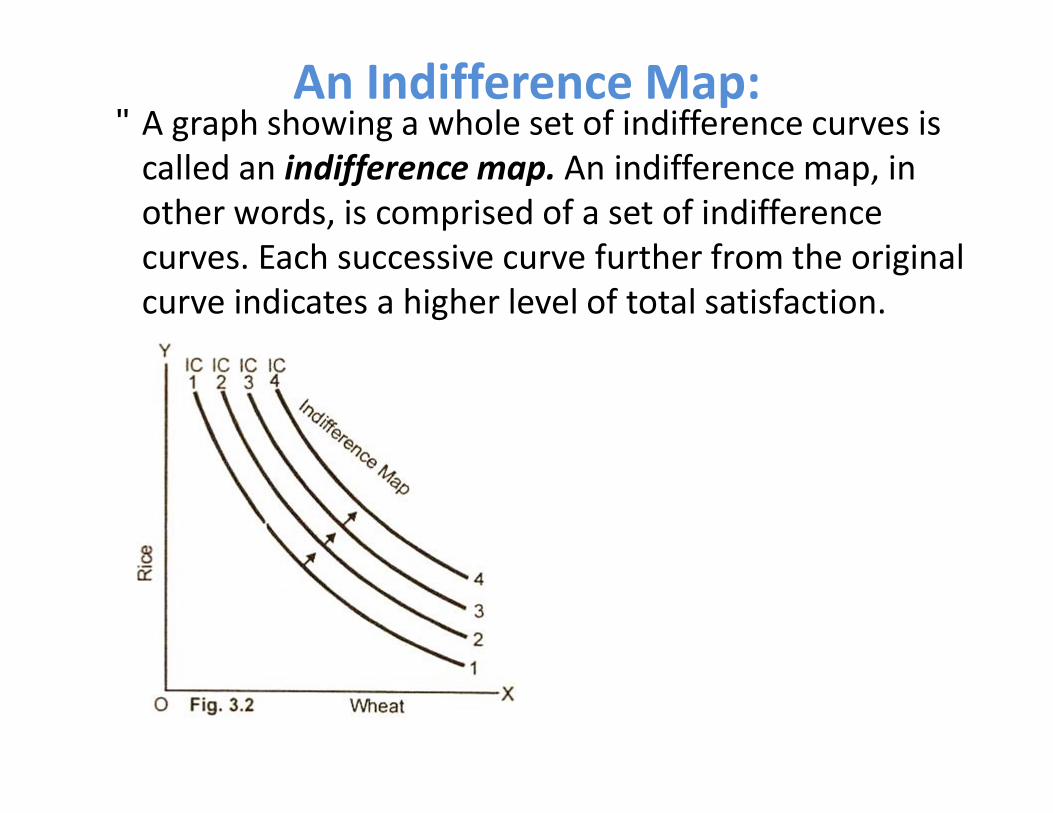
An Indifference Map:

• A graph showing a whole set of indifference curves is called an indifference map. An indifference map, in other words, is comprised of a set of indifference curves. Each successive curve further from the original curve indicates a higher level of total satisfaction.

Assumptions:

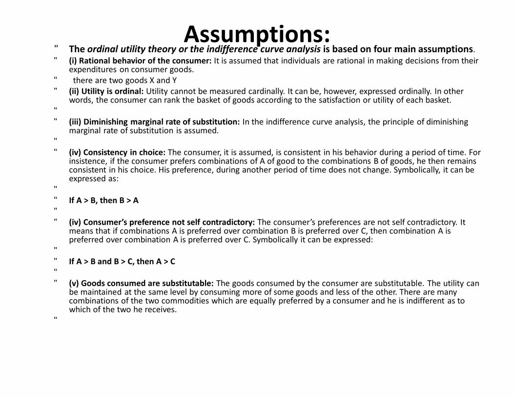
• The ordinal utility theory or the indifference curve analysis is based on four main assumptions. • (i) Rational behavior of the consumer: It is assumed that individuals are rational in making decisions from their

expenditures on consumer goods. • there are two goods X and Y • (ii) Utility is ordinal: Utility cannot be measured cardinally. It can be, however, expressed ordinally. In other

words, the consumer can rank the basket of goods according to the satisfaction or utility of each basket. • • (iii) Diminishing marginal rate of substitution: In the indifference curve analysis, the principle of diminishing

marginal rate of substitution is assumed. • • (iv) Consistency in choice: The consumer, it is assumed, is consistent in his behavior during a period of time. For

insistence, if the consumer prefers combinations of A of good to the combinations B of goods, he then remains consistent in his choice. His preference, during another period of time does not change. Symbolically, it can be expressed as:

• • If A > B, then B > A • • (iv) Consumer’s preference not self contradictory: The consumer’s preferences are not self contradictory. It

means that if combinations A is preferred over combination B is preferred over C, then combination A is preferred over combination A is preferred over C. Symbolically it can be expressed:

• • If A > B and B > C, then A > C • • (v) Goods consumed are substitutable: The goods consumed by the consumer are substitutable. The utility can

be maintained at the same level by consuming more of some goods and less of the other. There are many combinations of the two commodities which are equally preferred by a consumer and he is indifferent as to which of the two he receives.

•

Marginal Rate of Substitution (MRS): • Definition and Explanation:

• The concept of marginal rate substitution (MRS) was introduced by Dr. J.R. Hicks and Prof. R.G.D. Allen to take the place of the concept of diminishing marginal utility. Allen and Hicks are of the opinion that it is unnecessary to measure the utility of a commodity. The necessity is to study the behavior of the consumer as to how he prefers one commodity to another and maintains the same level of satisfaction.

• • For example, there are two goods X and Y which are not perfect substitute of each

other. The consumer is prepared to exchange goods X for Y. How many units of Y should be given for one unit of X to the consumer so that his level of satisfaction remains the same?

• • The rate or ratio at which goods X and Y are to be exchanged is known as the

marginal rate of substitution (MRS). In the words of Hicks: • • “The marginal rate of substitution of X for Y measures the number of units of Y that

must be scarified for unit of X gained so as to maintain a constant level of satisfaction”.

• • Marginal rate of substitution (MRS) can also be defined as: • • “The ratio of exchange between small units of two commodities, which are equally

valued or preferred by a consumer”. •

Formula:

• MRSxy = ∆Y ∆X • It may here be noted that the marginal rate of

substitution (MRS) is the personal exchange rate of the consumer in contrast to the market exchange rate.

•

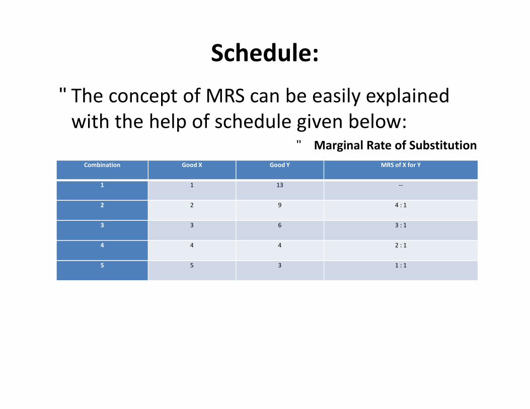
Schedule: • The concept of MRS can be easily explained

with the help of schedule given below: • Marginal Rate of Substitution

Combination Good X Good Y MRS of X for Y

1 1 13 --

2 2 9 4 : 1

3 3 6 3 : 1

4 4 4 2 : 1

5 5 3 1 : 1

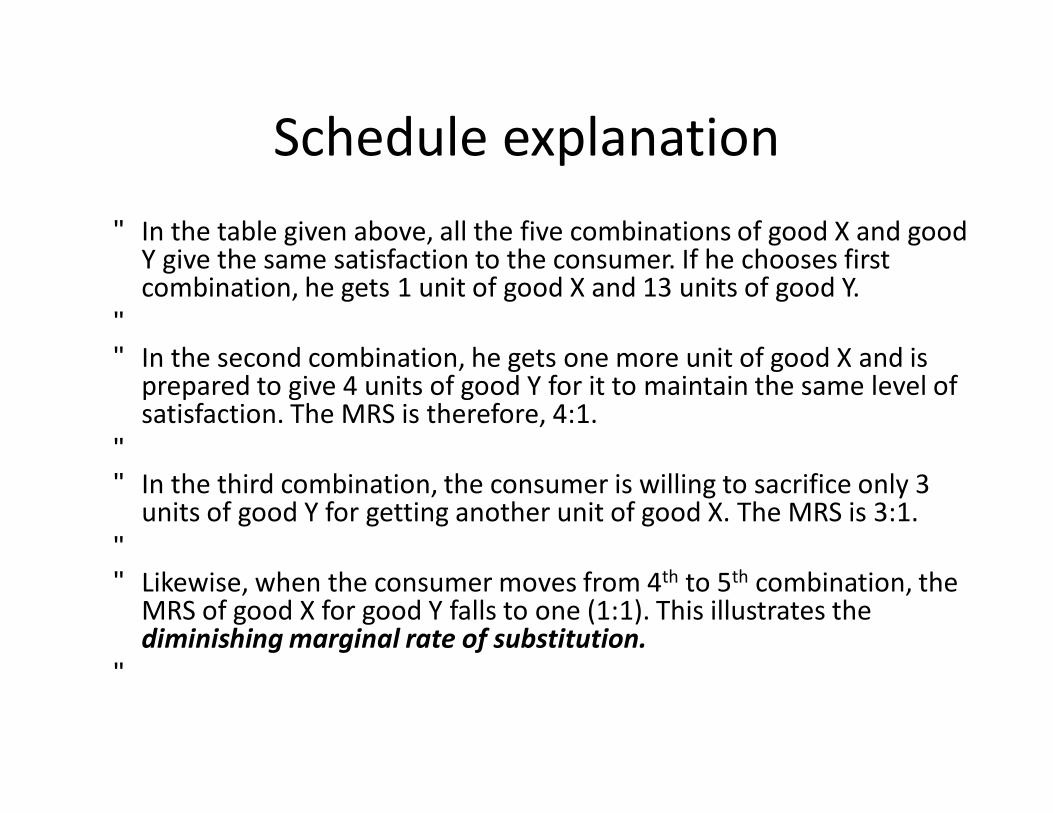
Schedule explanation • In the table given above, all the five combinations of good X and good

Y give the same satisfaction to the consumer. If he chooses first combination, he gets 1 unit of good X and 13 units of good Y.

• • In the second combination, he gets one more unit of good X and is

prepared to give 4 units of good Y for it to maintain the same level of satisfaction. The MRS is therefore, 4:1.

• • In the third combination, the consumer is willing to sacrifice only 3

units of good Y for getting another unit of good X. The MRS is 3:1. • • Likewise, when the consumer moves from 4th to 5th combination, the

MRS of good X for good Y falls to one (1:1). This illustrates the diminishing marginal rate of substitution.

•

Diminishing Marginal Rate of

Substitution: • In the above schedule, we have seen that as the consumer moves

from combination first to fifth, the rate of substitution of good X for good Y goes, down. In other words, as the consumer has more and more units of good X, he is prepared to forego less and less of good Y.

• • For instance, in the 2nd combination, the consumer is willing to give

4 units of good Y in exchange for one unit of good X, in the fifth combination only one unit of Y is offered for obtaining one unit of X.

• • This behavior showing falling MRS of good X for good Y and yet to

remain at the same level of satisfaction is known as diminishing marginal rate of substitution

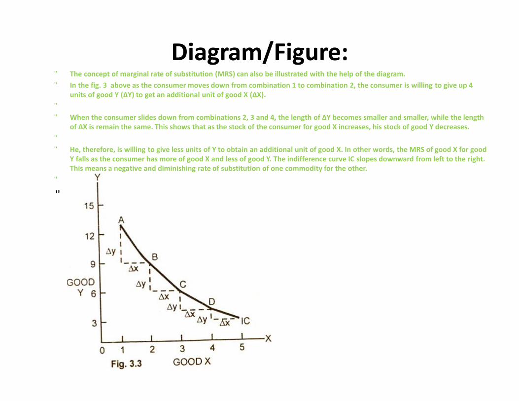
Diagram/Figure: • The concept of marginal rate of substitution (MRS) can also be illustrated with the help of the diagram.

• In the fig. 3 above as the consumer moves down from combination 1 to combination 2, the consumer is willing to give up 4 units of good Y (∆Y) to get an additional unit of good X (∆X).

• • When the consumer slides down from combinations 2, 3 and 4, the length of ∆Y becomes smaller and smaller, while the length

of ∆X is remain the same. This shows that as the stock of the consumer for good X increases, his stock of good Y decreases. • • He, therefore, is willing to give less units of Y to obtain an additional unit of good X. In other words, the MRS of good X for good

Y falls as the consumer has more of good X and less of good Y. The indifference curve IC slopes downward from left to the right. This means a negative and diminishing rate of substitution of one commodity for the other.

•

•

Importance of Marginal Rate of

Substitution (MRS): • (i) Measures utility ordinally: The concept of MRS is

superior to that of utility concept because it is more realistic and scientific than the theory of utility. It does not measure the utility of a commodity in isolation without reference to other commodities but takes into consideration the combination of related goods to which a consumer is interested to purchase.

• • (ii) A relative concept: The concept of marginal rate of

substitution has the advantage that it is relative and not absolute like the utility concept given by Marshall. It is free from any assumptions concerning the possibility of a quantitative measurement of utility

Exceptions of DMRS Law

• 1. Straight line indifference curve • L-shaped indifference curve

Properties/Characteristics of

Indifference Curve:

• Definition, Explanation and Diagram • An indifference curve shows combination of

goods between which a person is indifferent. The main attributes or properties or characteristics of indifference curves are as follows:

•

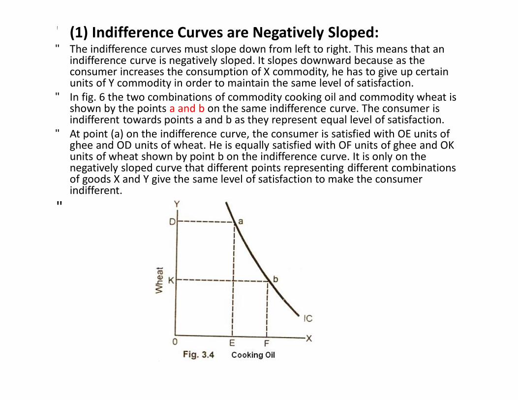
• (1) Indifference Curves are Negatively Sloped: • The indifference curves must slope down from left to right. This means that an

indifference curve is negatively sloped. It slopes downward because as the consumer increases the consumption of X commodity, he has to give up certain units of Y commodity in order to maintain the same level of satisfaction.

• In fig. 6 the two combinations of commodity cooking oil and commodity wheat is shown by the points a and b on the same indifference curve. The consumer is indifferent towards points a and b as they represent equal level of satisfaction.

• At point (a) on the indifference curve, the consumer is satisfied with OE units of ghee and OD units of wheat. He is equally satisfied with OF units of ghee and OK units of wheat shown by point b on the indifference curve. It is only on the negatively sloped curve that different points representing different combinations of goods X and Y give the same level of satisfaction to make the consumer indifferent.

•

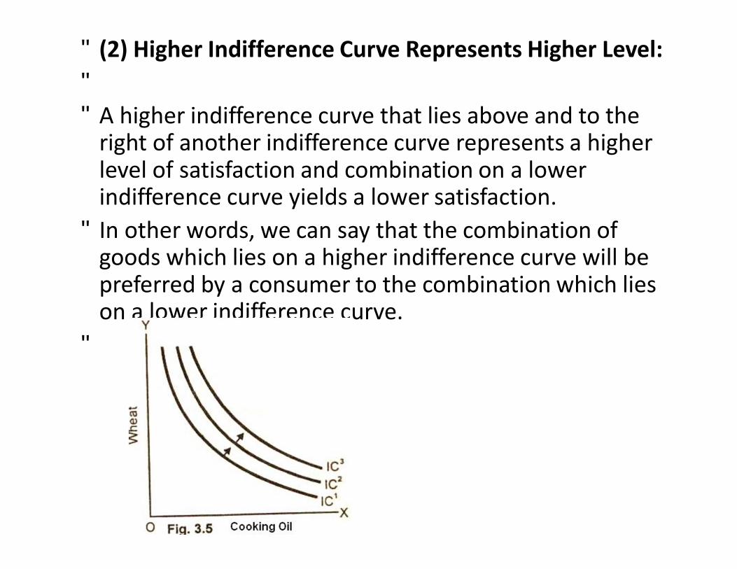
• (2) Higher Indifference Curve Represents Higher Level: • • A higher indifference curve that lies above and to the

right of another indifference curve represents a higher level of satisfaction and combination on a lower indifference curve yields a lower satisfaction.

• In other words, we can say that the combination of goods which lies on a higher indifference curve will be preferred by a consumer to the combination which lies on a lower indifference curve.

•

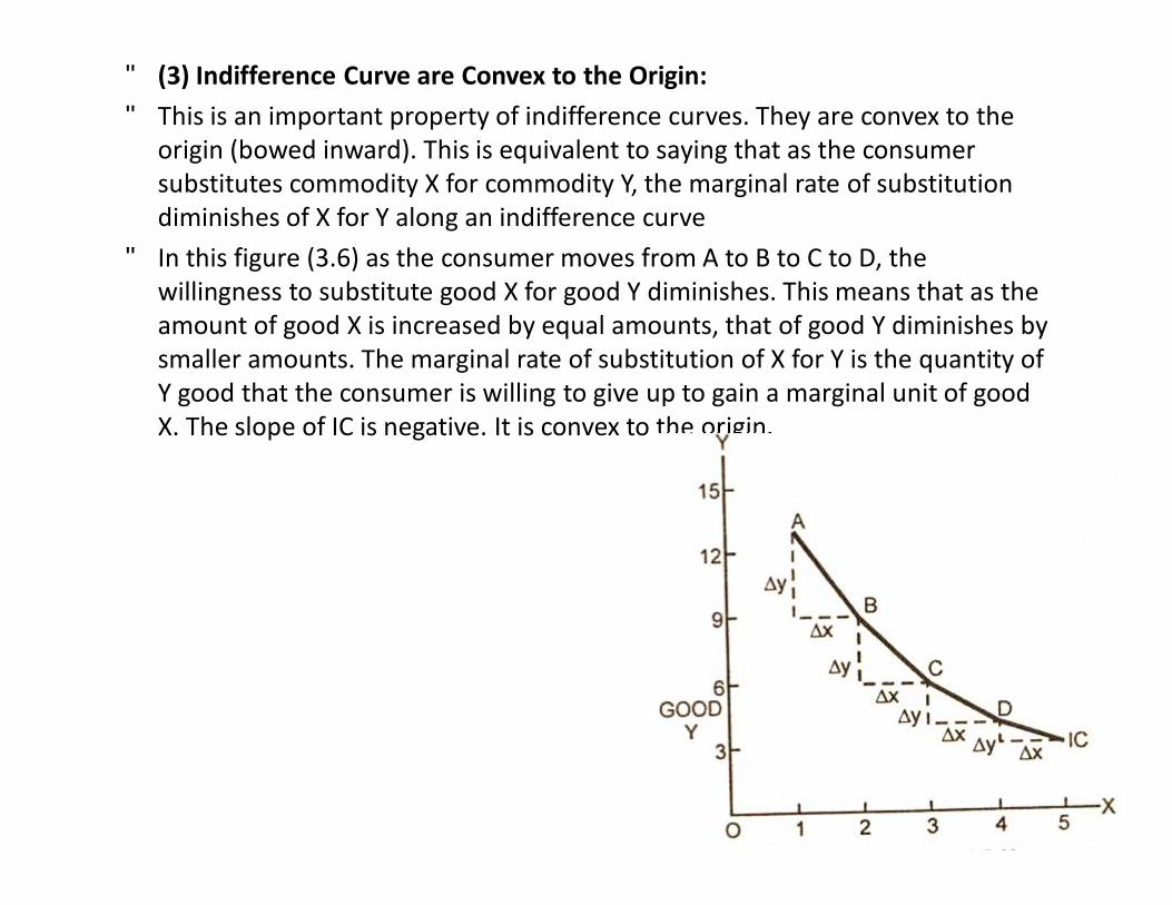
• (3) Indifference Curve are Convex to the Origin: • This is an important property of indifference curves. They are convex to the

origin (bowed inward). This is equivalent to saying that as the consumer substitutes commodity X for commodity Y, the marginal rate of substitution diminishes of X for Y along an indifference curve

• In this figure (3.6) as the consumer moves from A to B to C to D, the willingness to substitute good X for good Y diminishes. This means that as the amount of good X is increased by equal amounts, that of good Y diminishes by smaller amounts. The marginal rate of substitution of X for Y is the quantity of Y good that the consumer is willing to give up to gain a marginal unit of good X. The slope of IC is negative. It is convex to the origin.

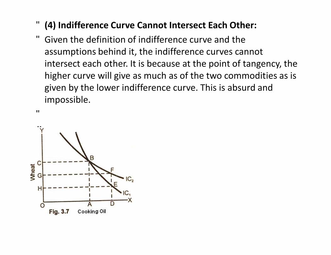
• (4) Indifference Curve Cannot Intersect Each Other: • Given the definition of indifference curve and the

assumptions behind it, the indifference curves cannot intersect each other. It is because at the point of tangency, the higher curve will give as much as of the two commodities as is given by the lower indifference curve. This is absurd and impossible.

•

•

• In fig 3.7, two indifference curves are showing cutting each other at point B. The combinations represented by points B and F given equal satisfaction to the consumer because both lie on the same indifference curve IC2. Similarly the combinations shows by points B and E on indifference curve IC1 give equal satisfaction top the consumer.

• • If combination F is equal to combination B in terms of satisfaction and

combination E is equal to combination B in satisfaction. It follows that the combination F will be equivalent to E in terms of satisfaction. This conclusion looks quite funny because combination F on IC2 contains more of good Y (wheat) than combination which gives more satisfaction to the consumer. We, therefore, conclude that indifference curves cannot cut each other.

• (5) Indifference Curves do not Touch the Horizontal or Vertical Axis: • • One of the basic assumptions of indifference curves is that the

consumer purchases combinations of different commodities. He is not supposed to purchase only one commodity. In that case indifference curve will touch one axis. This violates the basic assumption of indifference curves.

• •

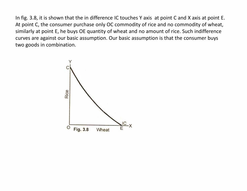
In fig. 3.8, it is shown that the in difference IC touches Y axis at point C and X axis at point E. At point C, the consumer purchase only OC commodity of rice and no commodity of wheat, similarly at point E, he buys OE quantity of wheat and no amount of rice. Such indifference curves are against our basic assumption. Our basic assumption is that the consumer buys two goods in combination.

• Important properties of indifference curves. • The above story suggests two important properties of indifference

curves • Indifference curves are downward sloping (they have negative

sloped). • Indifference curves are convex. That is the absolute value of their

slope declines as we obtain more X and less Y. • The above indifference curve was for all the bundles that give Mary

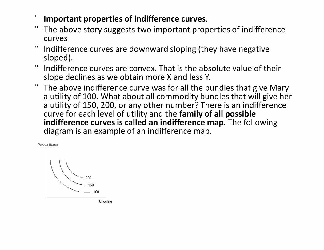
a utility of 100. What about all commodity bundles that will give her a utility of 150, 200, or any other number? There is an indifference curve for each level of utility and the family of all possible indifference curves is called an indifference map. The following diagram is an example of an indifference map.

• We can understand this diagram by looking at the point shown on the indifference curves. For example, our consumer is indifferent between bundles A and C but she prefers bundle B to both A and C. Also, whereas she is indifferent between E and D, she prefers both to B, A and C. As we talked earlier, with ordinal utility, the only relationships of interest are preference and indifference. The consumer prefers bundles on higher indifference curves to those on the lower curves and she is indifferent between bundles on the same curves.

Price Line or Budget Line:

• Definition and Explanation: • The understanding of the concept of budget line is essential for

knowing the theory of consumer’s equilibrium. • "A budget line or price line represents the various combinations

of two goods which can be purchased with a given money income and assumed prices of goods".

• The budget line is an important element analysis of consumer behavior. The indifference map shows people’s preferences for the combination of two goods. The actual choices they will make, however, depends on their income. The budget line is drawn as a continuous line. It identifies the options from which the consumer can choose the combination of goods.

• For example, a consumer has weekly income of $60. He purchases only two goods, packets of biscuits and packets of coffee. The price of each packet of biscuits is $6 and the price of each packet of coffee is $12. Given the assumed income and the price, of the two goods, the consumer can purchase various combination of goods or market combination of goods weekly.

•

Price Line or Budget Line cont----

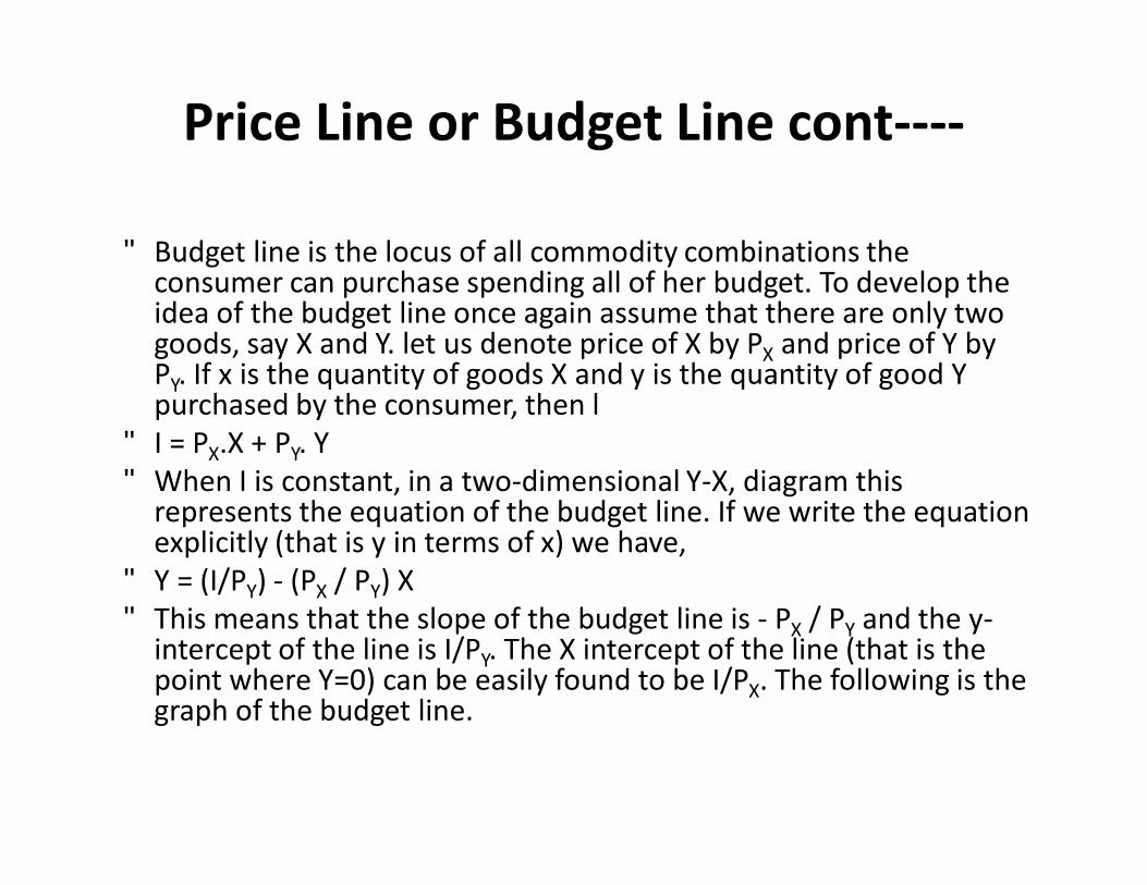
• Budget line is the locus of all commodity combinations the

consumer can purchase spending all of her budget. To develop the idea of the budget line once again assume that there are only two goods, say X and Y. let us denote price of X by PX and price of Y by PY. If x is the quantity of goods X and y is the quantity of good Y purchased by the consumer, then l

• I = PX.X + PY. Y • When I is constant, in a two-dimensional Y-X, diagram this

represents the equation of the budget line. If we write the equation explicitly (that is y in terms of x) we have,

• Y = (I/PY) - (PX / PY) X • This means that the slope of the budget line is - PX / PY and the y-

intercept of the line is I/PY. The X intercept of the line (that is the point where Y=0) can be easily found to be I/PX. The following is the graph of the budget line.

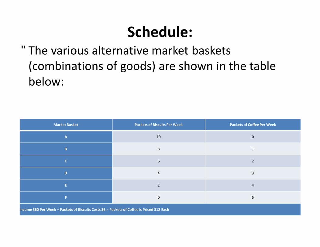
Schedule: • The various alternative market baskets

(combinations of goods) are shown in the table below:

Market Basket Packets of Biscuits Per Week Packets of Coffee Per Week

A 10 0

B 8 1

C 6 2

D 4 3

E 2 4

F 0 5

Income $60 Per Week = Packets of Biscuits Costs $6 = Packets of Coffee is Priced $12 Each

Schedule Cont----

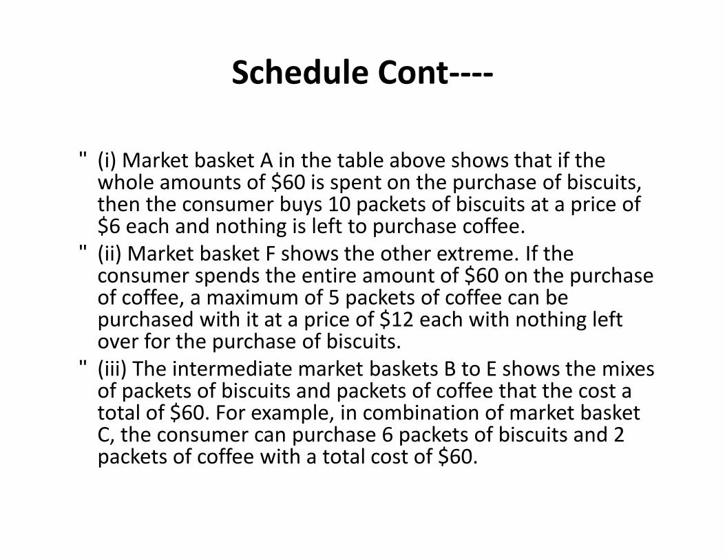
• (i) Market basket A in the table above shows that if the whole amounts of $60 is spent on the purchase of biscuits, then the consumer buys 10 packets of biscuits at a price of $6 each and nothing is left to purchase coffee.

• (ii) Market basket F shows the other extreme. If the consumer spends the entire amount of $60 on the purchase of coffee, a maximum of 5 packets of coffee can be purchased with it at a price of $12 each with nothing left over for the purchase of biscuits.

• (iii) The intermediate market baskets B to E shows the mixes of packets of biscuits and packets of coffee that the cost a total of $60. For example, in combination of market basket C, the consumer can purchase 6 packets of biscuits and 2 packets of coffee with a total cost of $60.

Diagram/Figure:

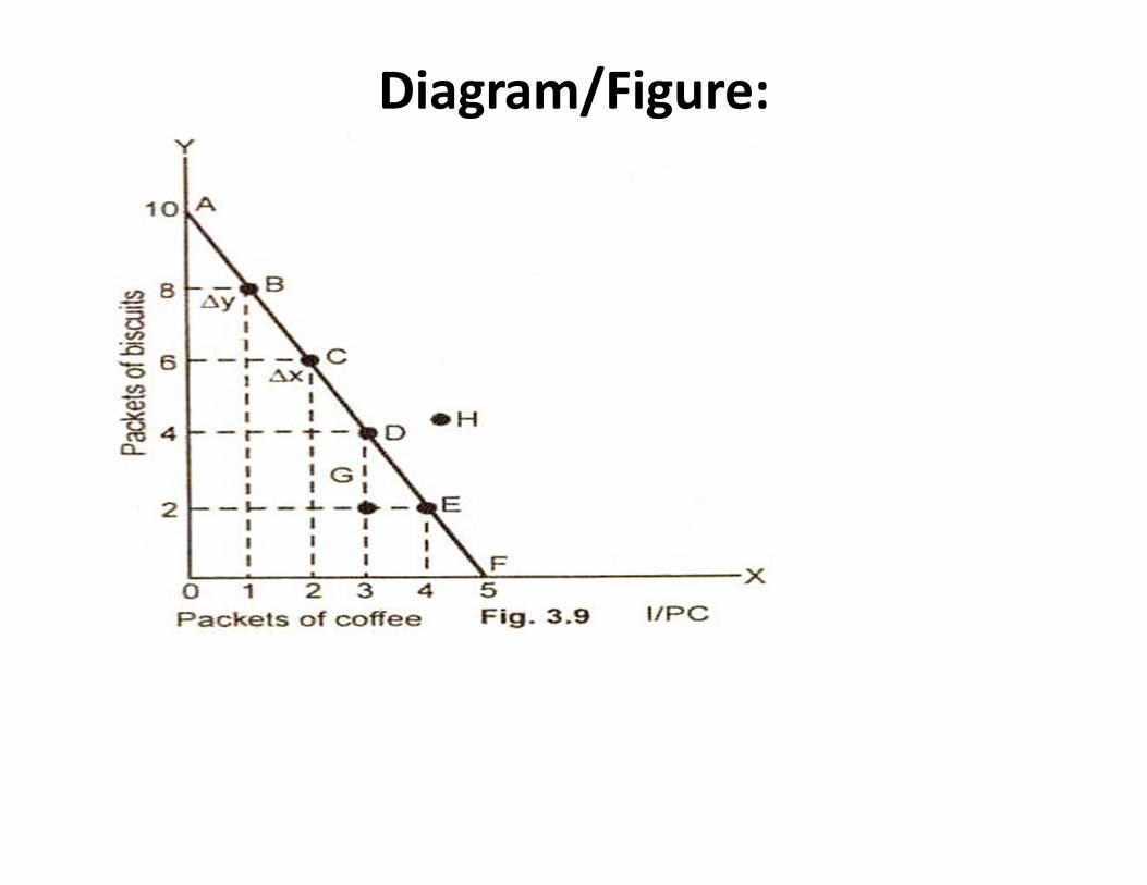
• In the fig. 3.9 the line AF shows the various combinations of goods the consumer can purchase. This line is called the budget line.

• • It shows 6 possible combinations of packets of biscuits and packets if coffee which a

consumer can purchase weekly. These combinations are indicated by points A, B, C, D, E and. Point A indicates that 10 packet of biscuits can be purchased if the entire income of $60 is devoted to the purchase of biscuits. Similarly, point F shows the purchase of 5 packets of coffee for the entire income of $60 per week.

• • The budget line AF indicates all the combinations of packets of biscuits and packets of

coffee which a consumer can buy given the assumed prices and income. In case, a consumer decides to purchase combination of goods inside the budget line such as G, then it involves a total outlay that is smaller then the amount of $60 per week. Any point outside the budget line such as H requires an outlay larger than the consumer’s weekly income of $60.

• • The slope of the budget line indicates how many packets of biscuits a purchaser must

give up to buy one more packet of coffee. For example, the slope at point B on the budget line is ∆Y / ∆X or two packets of biscuits 1 = packet of coffee. This indicates that a move from B to C involves sacrificing two packets of biscuits to gain an additional one packet of coffee. Since AF budget line is straight, the slope is constant at -2 packets of biscuits per one packet of coffee at all points along the line.

Shifts in Budget Line: • The price line is determined by the income of the consumer

and the prices of goods in the market. If there is a change in the income of the consumer or in the prices of goods, the price line shifts in response to a exchange in these two factors.

• • (i) Income changes: When there is change in the income of the

consumer, the prices of goods remaining the same, the price line shifts from the original position. It shifts upward or to the right hand side in a parallel position with the rise in income.

• • A fall in the level of income, product prices remaining

unchanged, the price line shifts left side from the original position. With a higher income, the consumer can purchase more of both goods than before but the cost of one good in terms of the other remains the same.

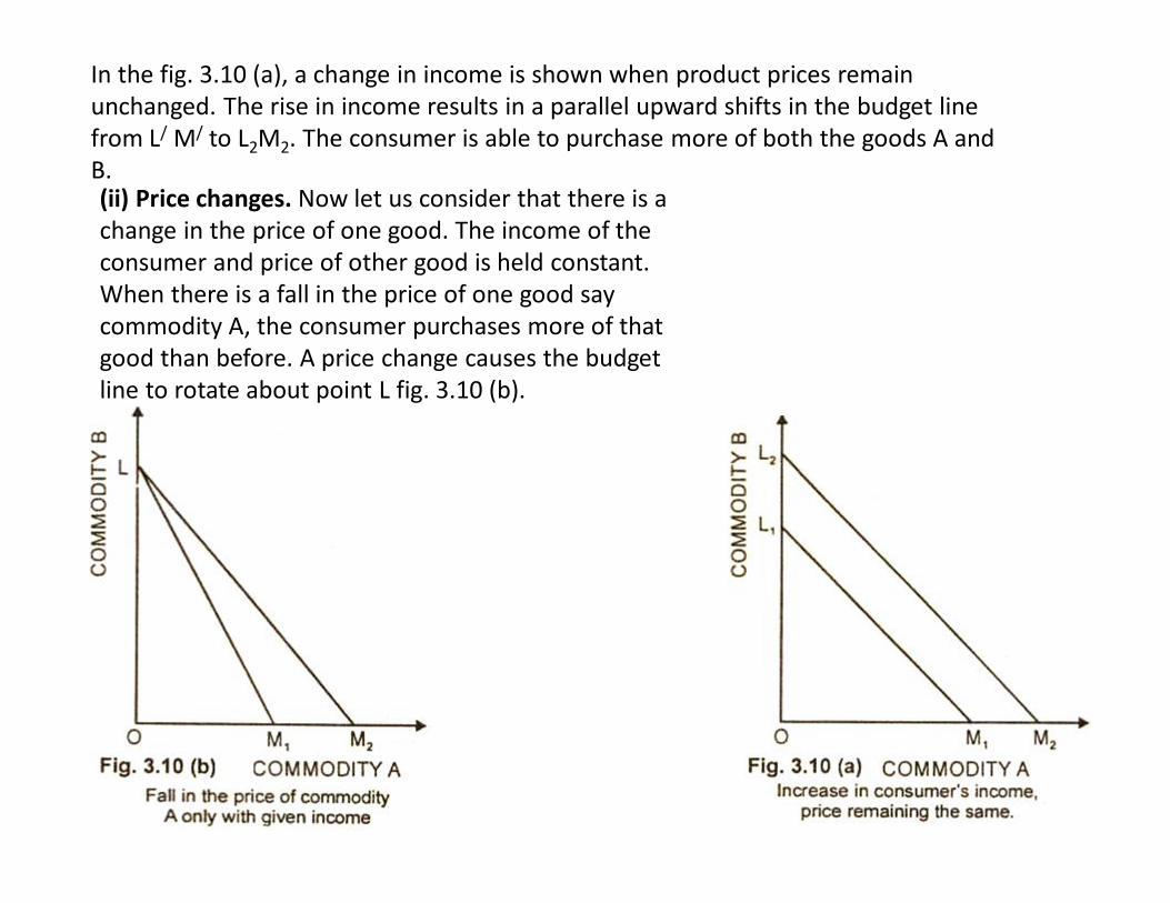
In the fig. 3.10 (a), a change in income is shown when product prices remain unchanged. The rise in income results in a parallel upward shifts in the budget line from L/ M/ to L2M2. The consumer is able to purchase more of both the goods A and B. (ii) Price changes. Now let us consider that there is a change in the price of one good. The income of the consumer and price of other good is held constant. When there is a fall in the price of one good say commodity A, the consumer purchases more of that good than before. A price change causes the budget line to rotate about point L fig. 3.10 (b).

Consumer's Equilibrium Through

Indifference Curve Analysis:

• Definition: • "The term consumer’s equilibrium refers to the

amount of goods and services which the consumer may buy in the market given his income and given prices of goods in the market".

• The aim of the consumer is to get maximum satisfaction from his money income. Given the price line or budget line and the indifference map:

• "A consumer is said to be in equilibrium at a point where the price line is touching the highest attainable indifference curve from below".

Conditions: • Thus the consumer’s equilibrium under the

indifference curve theory must meet the following two conditions:

• First: A given price line should be tangent to an indifference curve or marginal rate of satisfaction of good X for good Y (MRSxy) must be equal to the price ratio of the two goods. i.e.

• MRSxy = Px / Py • Second: The second order condition is that

indifference curve must be convex to the origin at the point of tangency.

Assumptions: • The following assumptions are made to determine the consumer’s equilibrium

position. • • (i) Rationality: The consumer is rational. He wants to obtain maximum satisfaction

given his income and prices. • • (ii) Utility is ordinal: It is assumed that the consumer can rank his preference

according to the satisfaction of each combination of goods. • • (iii) Consistency of choice: It is also assumed that the consumer is consistent in the

choice of goods. • • (iv) Perfect competition: There is perfect competition in the market from where the

consumer is purchasing the goods. • • (v) Total utility: The total utility of the consumer depends on the quantities of the

good consumed. • • Explanation: • The consumer’s consumption decision is explained by combining the budget line

and the indifference map. The consumer’s equilibrium position is only at a point where the price line is tangent to the highest attainable indifference curve from below.

Diagram/Figure:

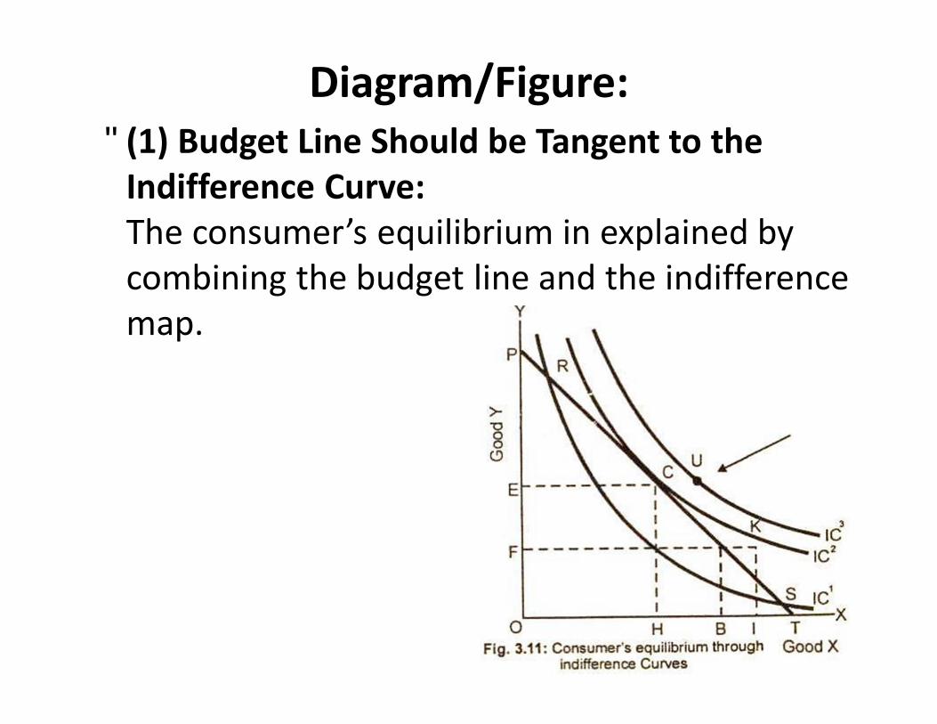
• (1) Budget Line Should be Tangent to the Indifference Curve: The consumer’s equilibrium in explained by combining the budget line and the indifference map.

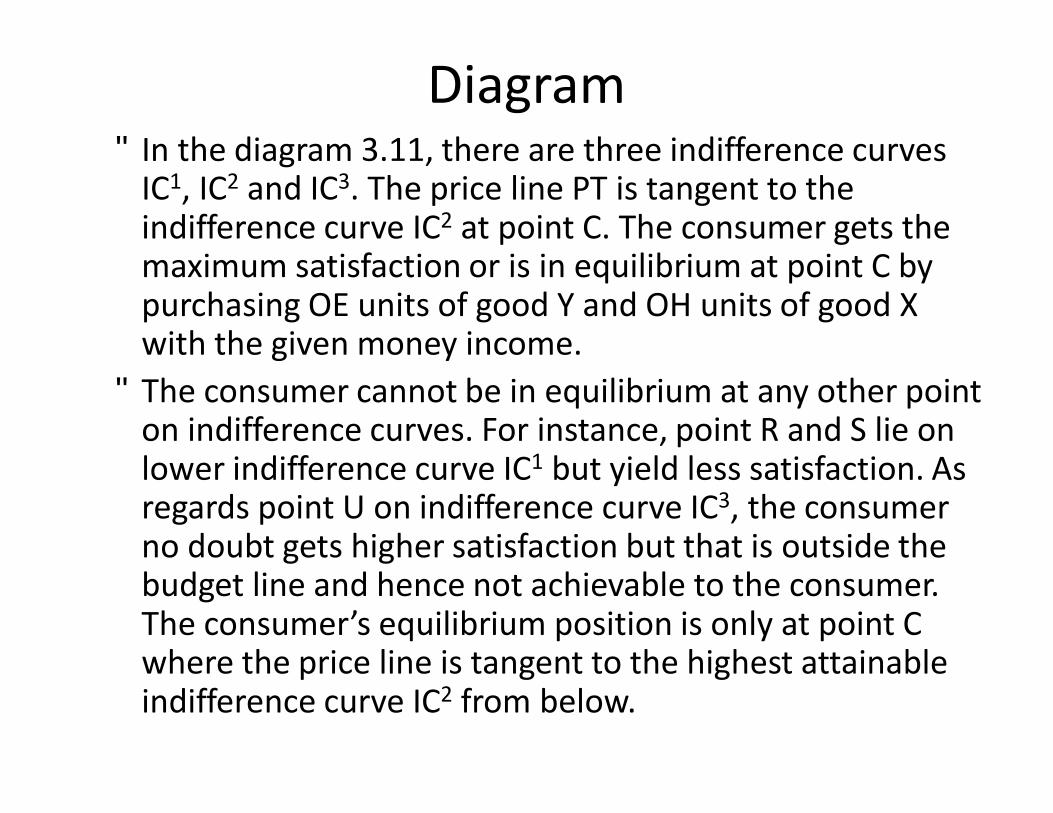
Diagram • In the diagram 3.11, there are three indifference curves

IC1, IC2 and IC3. The price line PT is tangent to the indifference curve IC2 at point C. The consumer gets the maximum satisfaction or is in equilibrium at point C by purchasing OE units of good Y and OH units of good X with the given money income.

• The consumer cannot be in equilibrium at any other point on indifference curves. For instance, point R and S lie on lower indifference curve IC1 but yield less satisfaction. As regards point U on indifference curve IC3, the consumer no doubt gets higher satisfaction but that is outside the budget line and hence not achievable to the consumer. The consumer’s equilibrium position is only at point C where the price line is tangent to the highest attainable indifference curve IC2 from below.

• (2) Slope of the Price Line to be Equal to the Slope of Indifference Curve: • The second condition for the consumer to be in equilibrium and get the

maximum possible satisfaction is only at a point where the price line is a tangent to the highest possible indifference curve from below. In fig. 3.11, the price line PT is touching the highest possible indifferent curve IC2 at point C. The point C shows the combination of the two commodities which the consumer is maximized when he buys OH units of good X and OE units of good Y.

• Geometrically, at tangency point C, the consumer’s substitution ratio is equal to price ratio Px / Py. It implies that at point C, what the consumer is willing to pay i.e., his personal exchange rate between X and Y (MRSxy) is equal to what he actually pays i.e., the market exchange rate. So the equilibrium condition being Px / Py being satisfied at the point C is:

• Price of X / Price of Y = MRS of X for Y • The equilibrium conditions given above states that the rate at which the

individual is willing to substitute commodity X for commodity Y must equal the ratio at which he can substitute X for Y in the market at a given price.

• (3) Indifference Curve Should be Convex to the Origin: • The third condition for the stable consumer equilibrium

is that the indifference curve must be convex to the origin at the point of equilibrium. In other words, we can say that the MRS of X for Y must be diminishing at the point of equilibrium. It may be noticed that in fig. 3.11, the indifference curve IC2 is convex to the origin at point C. So at point C, all three conditions for the stable-consumer’s equilibrium are satisfied.

• Summing up, the consumer is in equilibrium at point C where the budget line PT is tangent to the indifference IC2. The market basket OH of good X and OE of good Y yields the greatest satisfaction because it is on the highest attainable indifference curve. At point C:

• MRSxy = Px / Py

(1) Changes in Consumer's Equilibrium (Income Effect):

• Definition and Explanation: • We now describe in brief as to how indifference curves and budget lines can be used

to analysis the effects on consumption due to (a) changes in the income of a consumer (b) changes in the price of a commodity.

• In the consumer’s equilibrium analysis, it is primarily assumed that the price of the goods X and Y and the income of the consumer remains constant. We now examine as to how the consumer reacts as regards to his purchases of good when his income changes within the indifference curve frameworks. Income is one of the most important factors affecting the purchase of commodities.

• If the prices of goods, tastes and preferences of the consumer remains constant and there a change in his income, it will directly affect consumer’s demand. This effect on the purchase due to change in income is called the income effect.

• • A rise in consumer’s income will shift the price line or budget line upward to the

right and he goes on to higher point of equilibrium. A fall in the income, will shift the price line downward to the left and the consumer attains lower (tangency) points of equilibrium. The shift of the price line is parallel as the prices of the goods are assumed to remain the same. The income effect is explained with the help of following diagram.

•

Diagram/Figure:

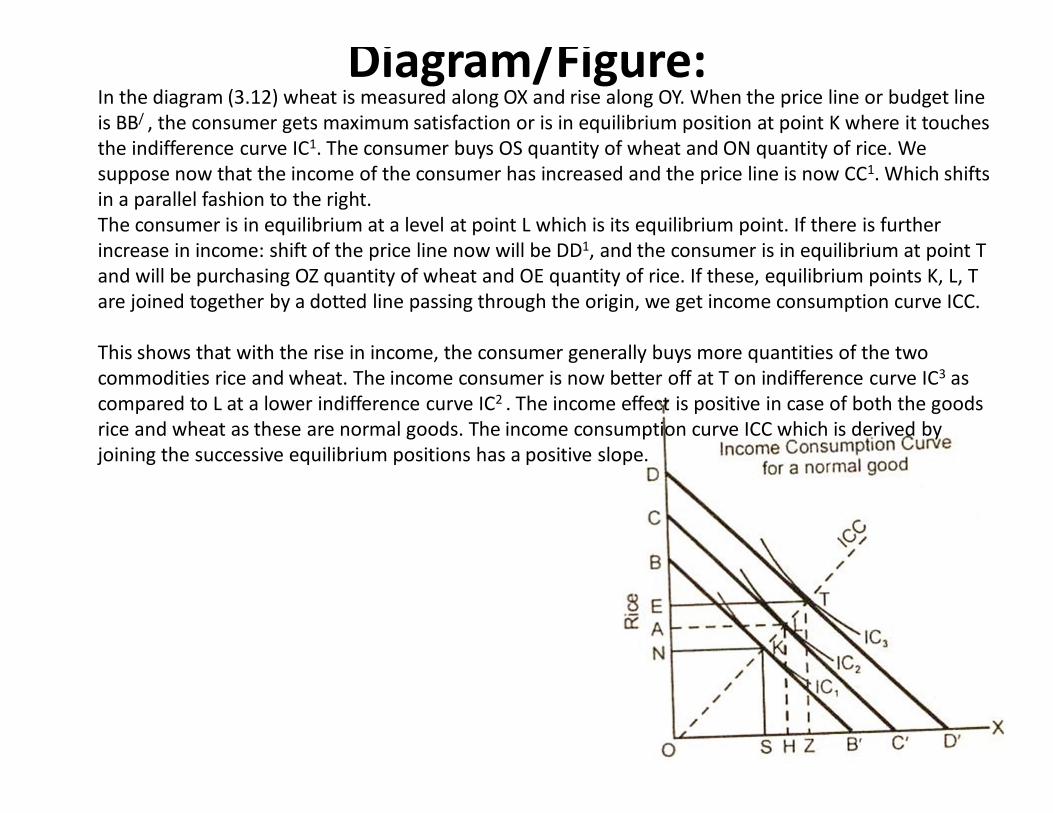
In the diagram (3.12) wheat is measured along OX and rise along OY. When the price line or budget line is BB/ , the consumer gets maximum satisfaction or is in equilibrium position at point K where it touches the indifference curve IC1. The consumer buys OS quantity of wheat and ON quantity of rice. We suppose now that the income of the consumer has increased and the price line is now CC1. Which shifts in a parallel fashion to the right. The consumer is in equilibrium at a level at point L which is its equilibrium point. If there is further increase in income: shift of the price line now will be DD1, and the consumer is in equilibrium at point T and will be purchasing OZ quantity of wheat and OE quantity of rice. If these, equilibrium points K, L, T are joined together by a dotted line passing through the origin, we get income consumption curve ICC. This shows that with the rise in income, the consumer generally buys more quantities of the two commodities rice and wheat. The income consumer is now better off at T on indifference curve IC3 as compared to L at a lower indifference curve IC2 . The income effect is positive in case of both the goods rice and wheat as these are normal goods. The income consumption curve ICC which is derived by joining the successive equilibrium positions has a positive slope.

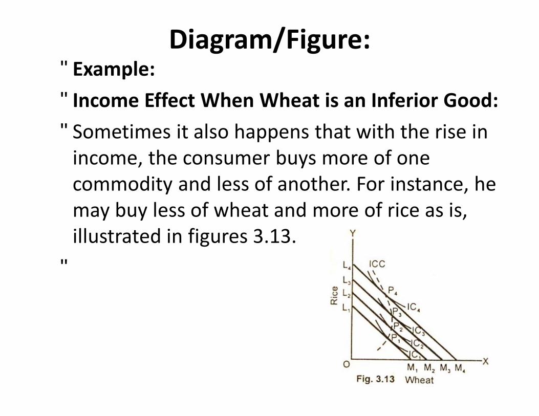
Diagram/Figure: • Example: • Income Effect When Wheat is an Inferior Good: • Sometimes it also happens that with the rise in

income, the consumer buys more of one commodity and less of another. For instance, he may buy less of wheat and more of rice as is, illustrated in figures 3.13.

•

• In diagram 3.13, the income consumption curve bends back on itself. With the rise in income, the consumer buys more of rice and less of wheat. The price effect for rice is positive and for wheat is negative. The good which is purchased less with the increase in income is called inferior good.

•

Income Effect When Rice is an Inferior

Good:

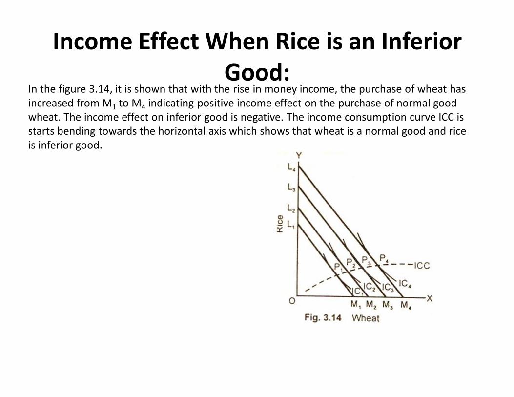
In the figure 3.14, it is shown that with the rise in money income, the purchase of wheat has increased from M1 to M4 indicating positive income effect on the purchase of normal good wheat. The income effect on inferior good is negative. The income consumption curve ICC is starts bending towards the horizontal axis which shows that wheat is a normal good and rice is inferior good.

(2) Changes in Consumer’s Equilibrium (Price Effect):

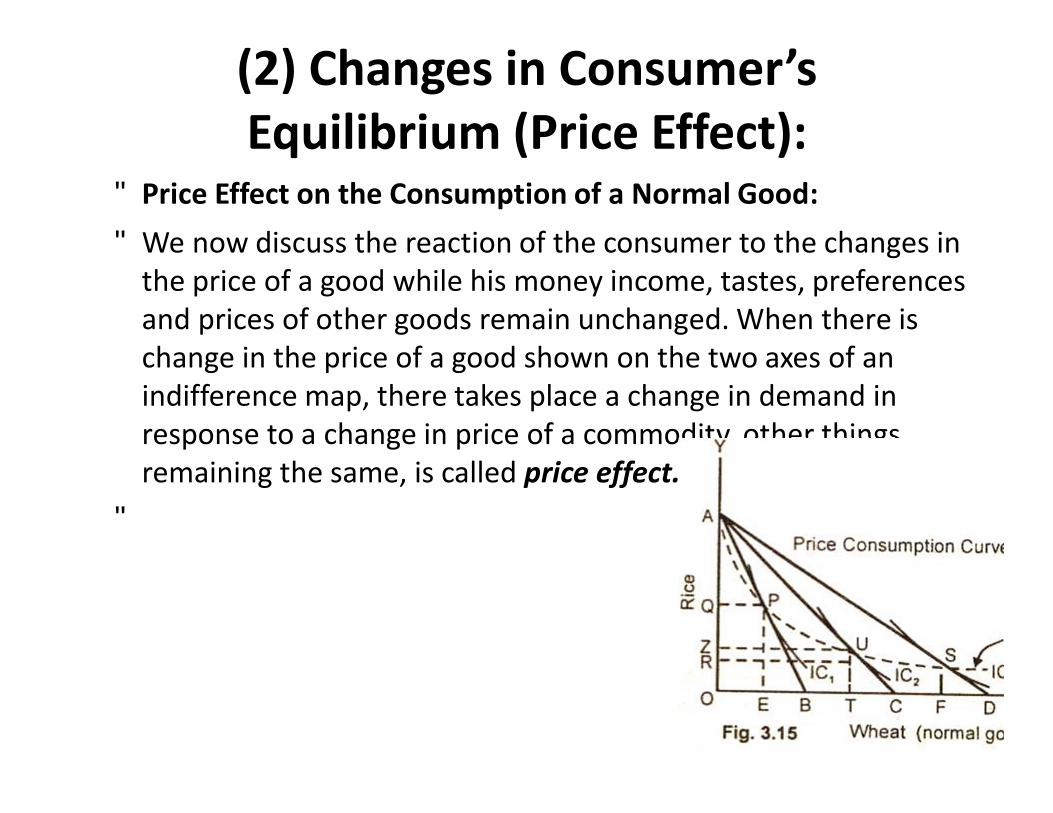
• Price Effect on the Consumption of a Normal Good: • We now discuss the reaction of the consumer to the changes in

the price of a good while his money income, tastes, preferences and prices of other goods remain unchanged. When there is change in the price of a good shown on the two axes of an indifference map, there takes place a change in demand in response to a change in price of a commodity, other things remaining the same, is called price effect.

•

(2) Changes in Consumer’s Equilibrium (Price Effect):

• For example in fig. 3.15, AB is the initial budget line. It is assumed that the price of wheat has fallen and the price of rice and the income of the consumer remains unchanged. The price line takes a new position AC and the equilibrium point shifts from P to U.

• • The consumer buys now OT quantity of wheat (the amount demanded

rises from OE to OT and OZ quantity of rice. With further fall in the price of wheat, the consumer is in equilibrium at point S, where the budget line AD is tangent to a higher indifference curve AC3. He buys now OF quantity of wheat and OR quantity of rice.

• • The rise in amount purchased of wheat (OE to OF) as a result of a fall in its

price is called price effect. The price effect on the consumption of a normal good is negative. If we join the equilibrium points PUS, we get price consumption curve (PCC) of the consumer for the commodity wheat

Price Effect When Commodity X is a Giffen Good:

• Giffen good is a particular type of inferior good. When there is a decrease in the quantity demanded of a good with a fall in its price, the good is called Giffen good after the name of Robert Giffen.

• • A British Economist Robert Giffen (1837-1910), observed that

sometimes it so happens that a decrease in the price of a particular good causes its quantity demanded to fall. The consumer spends the money he saves (by curtailing the demand) on the purchase of increased quantity of the other good. The decease in the price of Giffen good has an effect similar to an an increase in the income of a buyer. This particular type of behavior of the consumer to decrease demanded of good when its price falls is called Giffen Paradox.

• The price effect on the consumption of the Giffen good X is now explained with the help of diagram below:

•

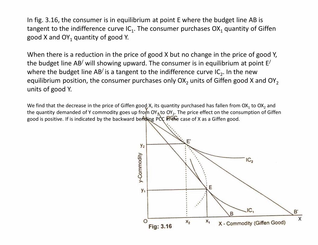
In fig. 3.16, the consumer is in equilibrium at point E where the budget line AB is tangent to the indifference curve IC1. The consumer purchases OX1 quantity of Giffen good X and OY1 quantity of good Y. When there is a reduction in the price of good X but no change in the price of good Y, the budget line AB/ will showing upward. The consumer is in equilibrium at point E/

where the budget line AB/ is a tangent to the indifference curve IC2. In the new equilibrium position, the consumer purchases only OX2 units of Giffen good X and OY2 units of good Y. We find that the decrease in the price of Giffen good X, its quantity purchased has fallen from OX1 to OX2 and the quantity demanded of Y commodity goes up from OY1 to OY2. The price effect on the consumption of Giffen good is positive. If is indicated by the backward bending PCC in the case of X as a Giffen good.

3) Consumer’s Equilibrium and the Substitution (Effect of Price Change):

• In the economic literature, there are two slightly different methods for explaining the impact of a price change on the quantity demanded of the two the two goods by the consumer. The first method is attributed to Hicks and Allen and is named as Hicks-Allen Substitution Effect.

• • The second put forward by S. Slutsky, a Russian

Economist, is known as Slutsky Substitution Effect. • • The two concept differ in the way in which real income

of the consumer is to be maintained constant when the substitution effect is to be observed. We explain the Hicks-Allen Method of tracing the substitution effect.

•

Hicks-Allen Substitution Effect: • In the Hicksian method, price changes is accompanied by so much

change in money income that the consumer is neither better off nor worse off than before. The money income is changed by an amount which keeps the consumer on the same indifference curve.

• • For instance, the price of good say X falls, and that of good Y remains

unchanged. With this fall in the price of good X, then the real income of the consumer would increase. This increase in the real income of the consumer is so withdrawn that he is neither better off nor worse off than above. The amount by which the money income is reduced is called compensating variation in income.

• • Substitution effect thus means the change in its relative price alone,

real income of the consumer remaining constant. The Hicksian substitution effect in now explained with the help of diagram below.

•

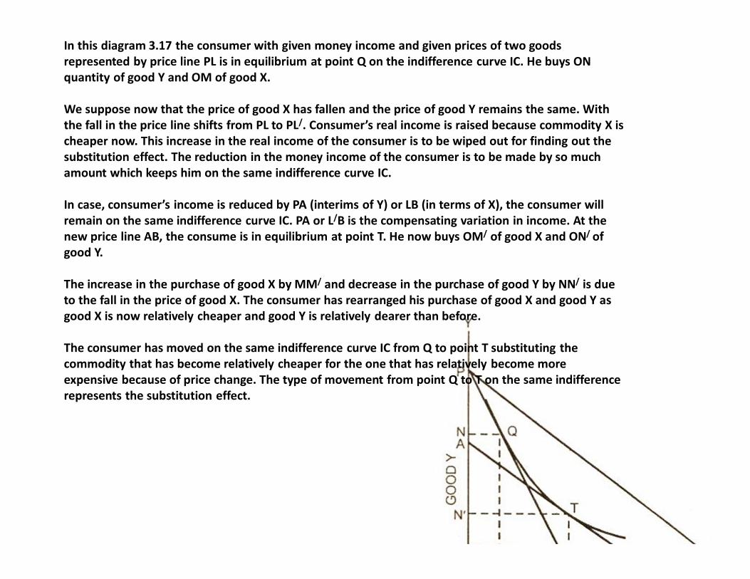
In this diagram 3.17 the consumer with given money income and given prices of two goods represented by price line PL is in equilibrium at point Q on the indifference curve IC. He buys ON quantity of good Y and OM of good X. We suppose now that the price of good X has fallen and the price of good Y remains the same. With the fall in the price line shifts from PL to PL/. Consumer’s real income is raised because commodity X is cheaper now. This increase in the real income of the consumer is to be wiped out for finding out the substitution effect. The reduction in the money income of the consumer is to be made by so much amount which keeps him on the same indifference curve IC. In case, consumer’s income is reduced by PA (interims of Y) or LB (in terms of X), the consumer will remain on the same indifference curve IC. PA or L/B is the compensating variation in income. At the new price line AB, the consume is in equilibrium at point T. He now buys OM/ of good X and ON/ of good Y. The increase in the purchase of good X by MM/ and decrease in the purchase of good Y by NN/ is due to the fall in the price of good X. The consumer has rearranged his purchase of good X and good Y as good X is now relatively cheaper and good Y is relatively dearer than before. The consumer has moved on the same indifference curve IC from Q to point T substituting the commodity that has become relatively cheaper for the one that has relatively become more expensive because of price change. The type of movement from point Q to T on the same indifference represents the substitution effect.

Comparison Between Indifference Curve Analysis and Marginal Utility

Analysis:

• There is difference of opinion among economists about the superiority of indifference analysis over cardinal utility analysis.

• Professor Hicks is of the opinion that the indifference analysis is more objective and scientific.

• Professor D.H. Rebertson is of the view that the Hicksian indifference curve technique is simply “old wine in new bottle”.

• • We give in brief the main points of similarly between these two types

of analysis and then discuss the superiority of Hicksian indifference curve analysis over the Marshallian Utility Approach.

•

Similarities Between the Two Approaches:

• (i) Rationality assumption: In the two approaches, it is assumed that the consumer behaves rationality for obtaining satisfaction from his expenditure on consumer goods. Marshall uses the term utility, and Hicks satisfaction.

• • (ii) Proportionality rule: The equilibrium condition of the consumer in both the analysis is the

proportionality rule. In cardinal utility analysis , the equilibrium condition of the consumer is: • • MUa / Pa = MUb / Pb = MUc / Pc …………. = MUn / Pn • • In the Hicksian analysis, this ratio of marginal utility has been substituted by marginal rate of substitution is: • • MRSxy

= Px / Py • • (iii) Diminishing MU and MRS: Another similarity between the two types of analysis is that both assume

that as the consumer gets more and more of a commodity, there is diminishing satisfaction to the consumer.

• • (iv) Same conclusion: The cardinal utility analysis and the Hicksian indifference curve analysis both reach at

the same conclusion about the consumer behavior. There is nothing new in the indifference approach.

Superiority of Hicksian Indifference Curve Analysis:

• i) It dispenses with cardinal measurement of utility: Professor R.G.D. Allen and J.R Hicks claims

that the indifference curve technique is scientific and more realistic than the Marshall’s utility analysis. The foundation of utility analysis is based, they say, on the cardinal utility function which assumes that the utility is measurable; whereas utility is purely subjective phenomena and cannot be exactly measured. It varies from person to person and time to time. Any effort to measure it precisely will be a futile one.

• • On the the other hand, the indifference approach is based on ordinal utility function, i.e., it does

not assign any number to a commodity , representing the amount of the utility. It simply assumes that the consumer weighs in his mind the relative desirability of the different combinations of goods and services.

• • (ii) It explains the income effect and price effect: Marshall assumes that the marginal utility of

money remains constant whereas the fact is that with a rise or fall in income, the marginal utility of the money changes. The indifference curve approach, however, takes into consideration the income effect changes in price of the commodity.

• • (iii) It studies combination of two goods: It assumed in the Marshallian utility analysis that a

consumer can measure the utility of a commodity in isolation from other commodities, i.e., it confines itself to a single commodity model. The indifference curve approach, on the other hand; studies combinations of two goods commodity and analysis the relationship of substitutable and complementarily.

•

• (iv) Application of the principle of MRS: The law of diminishing marginal utility has now been replaced by the principle of diminishing marginal rate of substitution. This law is more scientific and realistic and is well applicable in the field of consumption, production and distribution.

• (v) Popularity of indifference curve technique for the analysis of welfare economies: The indifference curve technique is more popular among the British economists and is mostly used for the analysis of welfare economies. For instance,

• the indifference curve approach helps us to explain that the direct tax imposes a lesser burden than an indirect tax upon the consumer.

• (a) The indifference curve approach helps us to explain that the direct tax imposes a lesser burden than an indirect tax upon the consumer.

• (b) The Hicksian indifference approach is also used for constructing the supply curve of labor in the country. We can explain with the help of indifference technique that when the wages of the workers rise, they begin to prefer leisure. For example, if wife and husband both work and the wages of the husband increases, wife often leaves the service and begins to do the domestic work.

• (c) The indifference curve technique is also used for illustrating the concept of consumer's surplus.

• (d) In case of rationing in the country, the indifference approach tells us that as the income and preferences of consumers differ, therefore, the goods should not be distributed equally. The income and tastes of the consumers should always be kept in view.

Criticism of Indifference Curve Approach:

• The indifference curve approach has been criticized on the following grounds: • (i) Old wine in new bottle: Professor D.H. Roberson is of the view that the difference between Marshallian

utility analysis and the indifference approach is that an old wine has been put in a new bottle. The only change which Hicks and Allen has made is that they have used the words marginal rate of substitution instead, of marginal utility.

• • (ii) Away from reality: The indifference curve technique is away from reality as the indifference hypothesis

are more complicated. • • (iii) Midway house: Schumpeter describes indifference analysis as a midway house as it particularly no

better than the utility analysis. • • (iii) The consumer is not rational: The consumer is not rational as he acts under various social, economic

and legal disabilities. • • (iv) Two goods model unrealistic: Two goods model unrealistic because a consumer buys large number of

commodities to satisfy his unlimited wants. • • (v) All commodities are not divisible: There is no doubt that indifference curve technique is not without

defects, but when we take into consideration the position as a whole, we find that the indifference approach is superior to that of utility approach because it is more realistic and less restrictive.

•