Journal of Mathematical Psychology 55 (2011) 379–385

Contents lists available at SciVerse ScienceDirect

Journal of Mathematical Psychology

journal homepage: www.elsevier.com/locate/jmp

Theory and tests of the conjoint commutativity axiom for additive conjointmeasurement✩

R. Duncan Luce, Ragnar Steingrimsson ∗

Institute for Mathematical Behavioral Sciences, University of California, Irvine, CA 92697-5100, United States

a r t i c l e i n f o

Article history:Received 17 January 2011Received in revised form25 May 2011Available online 25 June 2011

Keywords:Double cancellationThomsen conditionCommutativity ruleConjoint additivityConjoint commutativityMatchingLoudnessBrightnessAdditivityMeasurement

a b s t r a c t

The empirical study of the axioms underlying additive conjoint measurement initially focused mostlyon the double cancellation axiom. That axiom was shown to exhibit redundant features that madeits statistical evaluation a major challenge. The special case of double cancellation where inequalitiesare replaced by indifferences – the Thomsen condition – turned out in the full axiomatic context tobe equivalent to the double cancellation property but without exhibiting the redundancies of doublecancellation. However, it too has some undesirable features when it comes to its empirical evaluation,the chief among them being a certain statistical asymmetry in estimates used to evaluate it, namely twointerlocked hypotheses and a single conclusion. Nevertheless, thinking we had no choice, we evaluatedthe Thomsen condition for both loudness and brightness and, in agreement with other lines of research,we found more support for conjoint additivity than not. However, we commented on the difficulties wehad encountered in evaluating it. Thus we sought a more symmetric replacement, which as Gigerenzerand Strube (1983) first noted, is found in the conjoint commutativity axiom proposed by Falmagne (1976,who called it the ‘‘commutative rule’’). It turns out that, in the presence of the usual structural and othernecessary assumptions of additive conjoint measurement, we can show that conjoint commutativity isequivalent to the Thomsen condition, a result that seems to have been overlooked in the literature. Wesubjected this property to empirical evaluation for both loudness and brightness. In contrast to Gigerenzerand Strube (1983), our data show support for the conjoint commutativity in both domains and thus forconjoint additivity.

© 2011 Elsevier Inc. All rights reserved.

1. Background

Several recent studies (Luce, 2004, 2008; Steingrimsson, 2009;Steingrimsson & Luce, 2005a) have focused on whether or notsubjective measures of intensity over the two ears or two eyessatisfy the axioms for additive conjointmeasurementwhich lead toan additive numerical representation. A great deal of the relevantliterature such as Luce and Tukey (1964) was summarized inthe Foundations of Measurement (FofM) (Krantz, Luce, Suppes, &Tversky, 1971; Luce, Krantz, Suppes, & Tversky, 1990; Suppes,Krantz, Luce, & Tversky, 1989). The gist of that literature is that, inthe presence of various axioms (summarized inDefinition 7, p. 256,FofM I), additivity is forced if either of two properties is satisfied.Suppose that A and P are sets and that there is an ordering % overA × P . For a, b, c ∈ A and p, q, s ∈ P , the first property, called the

✩ Portions of this material have also appeared in Conference Proceedings of theMeeting of International Society for Psychophysics (Steingrimsson & Luce, 2010), inwhich we referred to Conjoint Commutativity as the Commutativity Rule.∗ Corresponding author.

E-mail address: ragnar@uci.edu (R. Steingrimsson).

0022-2496/$ – see front matter© 2011 Elsevier Inc. All rights reserved.doi:10.1016/j.jmp.2011.05.004

axiom of double cancellation, is

(a, p) % (b, q) and (c, q) % (a, s) (1)⇒ (c, p) % (b, s). (2)

The second axiom, called the Thomsen condition, is the special caseof double cancellation where % is replaced by ∼:

(a, p) ∼ (b, q) and (c, q) ∼ (a, s) (3)⇒ (c, p) ∼ (b, s). (4)

Gigerenzer and Strube (1983) pointed out why the consider-able redundancy of double cancellation (see below)makes it a veryunsatisfactory axiom to study empirically. Although the Thomsencondition avoids that redundancy, it necessarily exhibits a consid-erable statistical asymmetry (see below) whichmakes for an infer-ence difficulty.

The article is structured as follows.• We provide an overview of current tests of conjoint additivity

and an expanded discussion of the problems with testingdouble cancellation and the Thomsen condition.

• We provide a presentation of the conjoint commutativity prop-erty and a demonstration of how it offers a possible solution tothose problems.

380 R.D. Luce, R. Steingrimsson / Journal of Mathematical Psychology 55 (2011) 379–385

• We provide empirical evaluations of the conjoint commutativ-ity for both loudness and brightness.

A general comment: We are very aware that the measurementapproach we take here is not currently fashionable, having been‘‘replaced’’ by various process models. Unlike the measurementmodels for which the behavioral assumptions are directly testable,the process models are composed of unobservable, hypotheticalmechanisms. We feel that the added flexibility of processmodels comes at the (usually unacknowledged) very high costof unobservable mechanisms which, to this day, has not reallybeen resolved by such imaging techniques as fMRI. And we feelthat the very successful approach of four centuries of classicalphysics has not been given anything like a comparable effort inpsychology. The first author has devoted the last 12 years of hiscareer attempting to apply our knowledge of measurement todeveloping both psychophysical and utility measurement models,and collaboratingwith the second author andothers hehas focusedon experimental studies suggested by these models.

2. Current tests of conjoint additivity

Additivity over sense organs has been studied in a variety ofways; here, we focus on its axiomatic evaluation. As summarizedin Definition 7 of FofM I (p. 256), the test of additivity involves theevaluation of either double cancellation or the Thomsen condition.Double cancellation was explored by Levelt, Riemersma, and Bunt(1972), Falmagne (1976), Falmagne, Iverson, andMarcovici (1979),and Gigerenzer and Strube (1983) for loudness, by Schneider(1988) for loudness across critical bands, and by Legge and Rubin(1981) for perceived contrast; Ward (1990) evaluated doublecancellation for cross-modal additivity of loudness and brightness.The Thomsen condition was evaluated by Steingrimsson and Luce(2005a) for loudness and by Steingrimsson (2009) for brightness.Of these studies, two rejected double cancellation (Falmagne,1976; Gigerenzer & Strube, 1983).

Gigerenzer and Strube (1983) articulated clearly that doublecancellation involves the following type of redundancy. Supposethe signals are a, b, c, p, q, s for which double cancellation holds:

(a, p) % (b, q) and (c, q) % (a, s) ⇒ (c, p) % (b, s).

Then, for signals p′ and s′, with p′≻ p and s ≻ s′, we have, by

monotonicity, another version of double cancellation:

(a, p′) % (b, q) and (c, q) % (a, s′) ⇒ (c, p′) % (b, s′).

For example, they reported that ‘‘. . .no less than 82.64% of Leveltet al.’s data were defined a priori’’ in the sense that of acomplete factorial design they selected a subdesign from whichmonotonicity and transitivity implied the rest of the data.

So, in our empirical studies (Steingrimsson, 2009; Steingrims-son & Luce, 2005a), we focused instead on testing the non-redundant Thomsen condition:

(a, p) ∼ (b, q) and (c, q) ∼ (a, s) ⇒ (c, p) ∼ (b, s).

For both double cancellation and the Thomsen condition some ofthe signals are chosen by the experimenter and the rest by therespondent, as we next outline for the Thomsen condition.

In the experiments we have conducted, a stimulus pair (x, u)is taken to mean that an intensity x is presented to the left sensoryorgan, ear or eye, and intensity u is presented simultaneously to theright sensory organ, ear or eye. A match such as (a, p) ∼ (b, q) isone where (a, p) is judged to possess the same subjective intensityas does (b, q), i.e., (a, p) seems equally loud or equally brightas (b, q). An empirical match is one in which the experimenterselects a, b, and p and a respondent adjusts the intensity q in someway until a match is achieved. The q is in bold face to emphasize

that it is produced by a respondent and so varies over repeatedpresentations.

In this fashion, the Thomsen condition can be empiricallyevaluated in several different ways. One is to start with a, b, p, sand first estimate q such that

(a, p) ∼ (b, q). (5)

Next, estimate c such that

(c, q) ∼ (a, s). (6)

And finally, estimate c′ such that

(c′, p) ∼ (b, s). (7)

The empirical test is whether or not

c ∼ c′. (8)

A source of difficulty is that, in any straightforward testingmethod, the estimate c rests upon the estimate q, and so it hastwo sources of variability/bias, whereas c′ has only one source ofvariability/bias, where a bias may, for example, be a time-ordererror (arising from sequential presentation of stimulus pairs whichis inevitable in the auditory case).

Another possible source of difficulty relates to the fact that, inestimating q, c, and c′, typically the stimulus in one sensory organis adjusted while the stimulus in the other is held constant. Inaudition, this manipulation is experienced as a subjective changein the localization of a tone, whereas in brightness it is has nodirect subjective correlate. The fact is that Steingrimsson and Luce(2005a) found for loudness matches and Steingrimsson (2009)for brightness matches that the respondents required up to threetimes the amount of practice with this task before their judgmentsstabilized as compared to matches with equal adjustments in bothsensory organs. Thatmay be attributable to the difference betweenthe compound estimate and the simple one.

3. Equivalence of conjoint commutativity to the Thomsencondition

As first pointed out by Gigerenzer and Strube (1983), in an arti-cle on randomconjointmeasurement, Falmagne (1976) introducedthe following property, which he called the commutativity rule, andwhich we make more specific by speaking of conjoint commutativ-ity. With the function1 mp,q defined by

b = mp,q(a) iff (a, p) ∼ (b, q), (9)

conjoint commutativity asserts that

mp,q[mr,s(a)] = mr,s[mp,q(a)]. (10)

Note that, although Falmagne applied conjoint commutativityto random conjoint measurement, this property applies equallywell to the algebraic case. As far as we know, the literature has,with thenotable exception ofGigerenzer and Strube (1983),mostlyoverlooked the fact that conjoint commutativity can equally wellplay the role of the Thomsen condition, and has some advantagesover it.

Consider the part of Definition 7 of a binary conjoint structureonp. 256of Krantz et al. (1971) givenby the following assumptions.

A1 Weak ordering.A2 Monotonicity (= independence).A3 The Thomsen condition.

1 One can also use an operator notation instead of the function notation used byboth Falmagne and us.

R.D. Luce, R. Steingrimsson / Journal of Mathematical Psychology 55 (2011) 379–385 381

A4 Unrestricted solvability.2

A5 Archimedeaness.A6 Each component is essential.

Our main focus is on showing that we may use conjointcommutativity, which is statistically symmetric, instead of thestatistically asymmetric Thomsen condition. Assumptions A1, A2,and A5 are easily seen to be necessary properties that the orderingmust satisfy if there is an additive representation, andAssumptionsA4 and A6 are two non-necessary structural assumptions. Becausethe proof does notmake explicit use of the Assumptions other thanA3, we do not restate them here.

Theorem 1. Under Assumptions A1, A2, A4, A5 , and A6, thefollowing four properties are equivalent, and so either (i), (ii),or (iii) can play the role of A3

(i) Double cancellation.(ii) Thomsen condition.(iii) Conjoint commutativity (Falmagne, 1976).(iv) An interval scale, additive conjoint representation.

The proof is given in the Appendix.A clear advantage of conjoint commutativity is that it is

statistically symmetric in the sense that each side of (10) entailstwo respondent selected signals, which is not the case for eitherdouble cancellation or the Thomsen condition. It gains that atthe expense of having successive estimates on each side of thenull hypothesis. It does not, however, address the potential issuethat may arise in empirically producing a match by adjusting theintensity in one sensory organwhile keeping the intensity constantin the other organ. (Note: we will nevertheless attempt to addressthis final issue methodologically by varying the sensory organ inwhich the variable tone is presented).

Conjoint commutativity has, to the best of our knowledge, beenempirically evaluated only by Gigerenzer and Strube (1983). Theyevaluated a probabilistic version and rejected it for loudness. Here,conjoint commutativity, (10), is evaluated in an algebraic form intwo domains, loudness and brightness, presented as Experiment 1and Experiment 2, respectively.

3.1. General method

The experiments have several common testing features, whichnow outline.

3.1.1. RespondentsA total of nine students at the University of California, Irvine,

and one coauthor3 participated in the two experiments. Allrespondents who provided loudness data reported normal hearingand those who provided brightness data reported corrected-to-normal vision. Except for the coauthor, each respondent received$12 per session. Each person provided written consent and wastreated in accord with the ‘‘Ethical Principles of Psychologistsand Code of Conduct’’ (American Psychological Association, 2002).Consent forms and procedures were approved by UC Irvine’sInstitutional Review Board.

2 Definition 7, FofM I only needed restricted solvability, but to be sure that wecan always deal with the constructions for conjoint commutativity, we need theunrestricted version of solvability.3 This we judged acceptable because knowledge of the experimental design does

not change the sensations onwhich the behavioral tasks of matching are based. Thecoauthor is numbered R22.

3.1.2. Notational conventionSound intensities are reported in dB SPL (dB for short) and

light intensities in cd/m2. The theory, however, is cast in termsof intensity increments above threshold intensity. Therefore, witha threshold of xτ for the left ear/eye and a threshold of uτ forthe right ear/eye, the effective stimulus (x, u) has x = x′

−

xτ and u = u′− uτ , where (x′, u′) are the actual intensities

presented. However, because all signals werewell above thresholdand the respondentswere selected for their normal hearing/vision,the error in reporting intensities (x′, u′), using dB or cd/m2, isnegligible.

3.1.3. Statistical methods and presentation of resultsThe goal of our experiments is to evaluate our evidence for

parameter-free null-hypotheses that have the generic form Lside =

Rside. Since we have no a priori model of how individuals relate, alldata analysis is done on individual data (e.g., Luce, 1995, p. 20).And, because we have no a priori model of the distribution ofthe data, we use the non-parametric Mann–Whitney U (M–WU) test at the 0.05 level. This is the choice of numerous otherpapers (e.g., Falmagne (1976); Gigerenzer and Strube (1983);Ellermeier and Faulhammer (2000); Zimmer, Luce, and Ellermeier(2001); Ellermeier, Narens, and Dielmann (2003), Zimmer (2005);Steingrimsson and Luce (2005a); Steingrimsson and Luce (2005b);Steingrimsson and Luce (2006); Steingrimsson and Luce (2007);Steingrimsson (2009); Luce, Steingrimsson, and Narens (2010);Steingrimsson (2011)).

As the estimation steps are made in discrete steps (see theProcedure section) and the estimates appear reasonably symmet-ric, the mean is known to be a good estimate for the median. Inloudness, we report and collect data using dB values, whereas inbrightness the stimuli and data are in LUT (themonitor’s video cardLook Up Table of integer values 0–255) values, but are reported inunits of cd/m2. This involves a power transform, and so we reportthe transformed mean LUT values as well as the normalized stan-dard deviations (maintaining the relative magnitude vis-a-vis themean in cd/m2).4

3.1.4. ProcedureEmpirical evaluation of the conjoint commutativity, (10), in-

volves obtaining several matches of the generic form (x, u) ∼

(z, v), where the z is under respondent control and x, u, and v aresignals selected by the experimenter. The general procedure is avariation on the method of adjustment in which the respondent isfree to adjust the intensity of z up or down as often as desired un-til satisfied with the match, which is called z. Concretely, respon-dents could choose any of four changes in intensity described asextra-small, small, medium, and large. In the loudness case, theycorresponded to .5, 1, 2, or 4 dB, and in the brightness case theycorresponded to luminance steps of 1, 2, 4, or 8 LUT values. Fol-lowing an adjustment, the stimuli were next presented with therequested adjustment included. The respondent repeated this pro-cess until satisfied with the match, which was indicated by press-ing a different key, afterwhich the nextmatching task commenced.

Experiments were conducted in sessions of at most one hourduration. The initial session was devoted to obtaining writtenconsent, explaining the task, and running practice trials. Allrespondents trained for one additional session. Rest periods wereencouraged, but both their frequency and duration were under therespondent’s control.

The following four matches were needed to evaluate the con-joint commutativitymp,q[mr,s(a)] = mr,s[mp,q(a)].

4 We thank Dr. J. Yellott for this suggestion.

382 R.D. Luce, R. Steingrimsson / Journal of Mathematical Psychology 55 (2011) 379–385

1. (a, r) ∼ (b, s): The respondent produces b = mr,s(a).2. (b, p) ∼ (d, q): The intensity b is obtained in step 1, the

respondent produces d = mp,q(b).3. (a, p) ∼ (c, q): The respondent produces c = mp,q(a).4. (c, r) ∼ (e, s): The intensity c is obtained in step 3, the

respondent produces e = mr,s(c).The property is said to hold when the hypothesis that d ∼ e is

not rejected.In steps 1–4, note that all adjustments are made in the left

sensory organ. The property can equally well be evaluated byits mirror image in which b = m′

p,q(a) iff (p, a) ∼ (q, b),and the conjoint commutativity is then given by m′

p,q[m′r,s(a)] =

m′r,s[m

′p,q(a)]. The four matches required for these are referred to

as steps 5–8, and are analogous to steps 1–4.Note: If the sensations evoked from physically identical in-

puts to the two ears/eyes were identical, then they would be be-haviorally interchangeable. However, such symmetry has beenunequivocally rejected for both loudness (Steingrimsson & Luce,2005a) and brightness (Steingrimsson, 2009). This means thatm′

p,q(a) = mp,q(a), and thus m and m′ constitute different experi-mental conditions. An additional empirical result of Steingrimssonand Luce (2005a) was that this non-symmetry of the ears was notbehaviorally constant but could be affected by, for example, sus-tained matching in one of the two ears within a session, a resultSteingrimsson and Luce (2006) described using a form of a filter-ing model.

One plausible consequence of Steingrimsson and Luce’s (2006)filtering model is that a bias formed by consistently matching atone in one ear may be counteracted by mixing within a blockof trials the sensory organ to which the variable stimulus ispresented. This can be accomplished by mixing the trials of steps1–4 and 5–8 within a block, and hence we did that. This plausiblyaddresses, by experimental methodology, the remaining problemwith evaluating additivity.

The eight matches (1–8) were run in a block of trials generatingtwo tests of the conjoint commutativity. Respondents typicallycompleted 10 blocks per (one-hour) session. Thus, in additionto a practice session, three experimental sessions were requiredto obtain the typical 30 estimates collected for each matchingcondition.

3.2. Experiment 1: Loudness

3.2.1. MethodStimuli and equipment: The tones, x to the left ear and u to the

right, were 1 kHz sinusoids of 100 ms duration which included10 ms on and 10 ms off ramps. For a match such as (x, u) ∼

(z, v), the two joint presentations were separated by 450 ms.The stimuli were generated digitally using a personal computerand played through a 24-bit digital-to-analog converter (RP2.1Real-time processor, Tucker–Davis Technology). The intensity andfrequency were controlled using a programmable interface forthe RP2.1, and stimuli were presented over Sennheiser HD265Lheadphones to the respondent seated in an individual, single-walled IAC sound booth located in a quiet laboratory room. A safetyceiling of 90 dB was imposed in all experiments.

Loudness matching and the stimulus conditions: For the loudnessmatch (x, u) ∼ (z, v), the initial intensity for z is chosen by theexperimenter at random in a 10 dB interval around a best guessfor its final estimate. Listed in Table 1 are the stimulus valuesfor the two conditions under which conjoint commutativity wasevaluated in loudness.

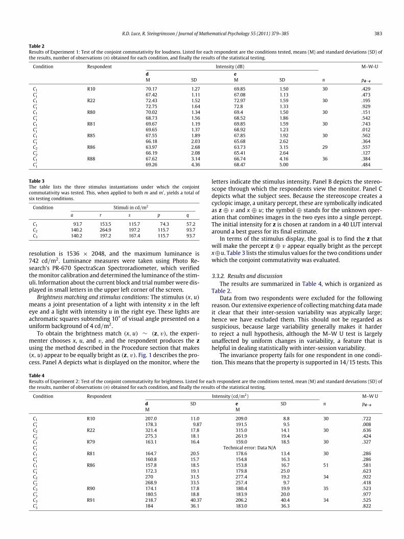
3.2.2. Results and discussionThe results are summarized in Table 2. For each respondent, the

columns are themeans and standard deviations ford and e, and the

Table 1The table lists the two stimulus instantiations under which the conjointcommutativity was tested, which, when applied to both m and m′ , resulted in fourtesting conditions.

Condition Stimuli (dB)a r s p q

C1 64 70 67 66 58C2 60 66 67 68 62

number of observations, n, for each sample. The statistics columnreports theM–WU test of the null hypothesis d ∼ e, given as pd∼e.

For R81, the C ′

1 condition fails. Otherwise, the property is foundto be supported in 13/14 tests. We regard this to be reasonablystrong evidence in favor of the property, and, as a consequence,evidence favoring an additive conjoint representation in loudness.This result mirrors the conclusion of Steingrimsson and Luce(2005a) about additivity, but is at odds with the results ofGigerenzer and Strube (1983), who evaluated double cancellationand conjoint commutativity and rejected both. Steingrimsson andLuce (2005a) discussed in some detail the discrepancy betweenthe double cancellation and their favorably evaluated Thomsencondition. In comparing the test of conjoint commutativity,two major differences emerge (these were also discussed bySteingrimsson and Luce (2005a)). First, Gigerenzer and Strube(1983) used an experimental technique in which the estimatedmedian of the observations in the first estimate, hereb, was used asan input in a subsequent evaluation in the second step (obtainingd). This has three consequences: namely, any bias in the estimateof themedianwill pass on into the second estimation step, the firstpart of a session is devoted to the first step and the second part tothe second step, risking inter-session bias (frequently observed),and the variance from the first step does not accumulate into thesecond step. Here, we avoid all three by using each estimatedinstance of b as input in the following step (see trial types 2and 6). This methodology allows all trial types to appear withina block of trials, reduces the risk of step one being based ona bias in median estimation, and preserves variability throughboth estimation steps. Indeed, the second major difference is thatGigerenzer and Strube (1983) found a statistically significant biassuch that d > e (and similarly for double cancellation) whereaswe do not observe such a bias in our results. Finally, it maybe important that Gigerenzer and Strube (1983) collected fewerobservations of e and d (20) than of b and d (41) – this theydid to fit data collection within a session – whereas we collectedequal numbers of both, and typically 30 or more, and, due themixing of all trials in a block with a session consisting of typically8–10 blocks, we could pool data across sessions, which, under theassumption of uniform variance within a session, is accounted forby the use of the M–W U test statistic. Finally, we used tones of100 ms in duration all at 1 kHz, whereas Gigerenzer and Strube(1983) used 4 s presentation of reference pairs and tones of 200 Hzand 6 kHz, respectively. All these differences are both substantiveand substantial enough plausibly to account for the difference inresults.

3.3. Experiment 2: Brightness

3.3.1. MethodStimuli and equipment: The experiment was conducted in a

dark room, and each respondent received a minimum of 10 minof dark adaptation. The stimuli were generated by a personalcomputer and displayed on a monitor (Eizo RadiForce RX320)with an automatic luminance uniformity equalizer and black-light sensor to compensate for luminance fluctuation caused byambient temperature and passage of time as well as build ingamma correction. The diagonal size is 54 cm, the maximum

R.D. Luce, R. Steingrimsson / Journal of Mathematical Psychology 55 (2011) 379–385 383

Table 2Results of Experiment 1: Test of the conjoint commutativity for loudness. Listed for each respondent are the conditions tested, means (M) and standard deviations (SD) ofthe results, number of observations (n) obtained for each condition, and finally the results of the statistical testing.

Condition Respondent Intensity (dB) M–W-Ud eM SD M SD n pd∼e

C1 R10 70.17 1.27 69.85 1.50 30 .429C ′

1 67.42 1.11 67.08 1.13 .473C1 R22 72.43 1.52 72.97 1.59 30 .195C ′

1 72.75 1.64 72.8 1.33 .929C1 R80 70.02 1.34 69.4 1.50 30 .151C ′

1 68.73 1.56 68.52 1.86 .542C1 R81 69.67 1.19 69.85 1.59 30 .743C ′

1 69.65 1.37 68.92 1.23 .012C1 R85 67.55 1.89 67.85 1.92 30 .562C ′

1 66.18 2.03 65.68 2.62 .364C2 R86 63.97 2.68 63.73 3.15 29 .557C ′

2 66.19 2.08 65.41 2.64 .127C1 R88 67.62 3.14 66.74 4.16 36 .384C ′

1 69.26 4.36 68.47 5.00 .484

Table 3The table lists the three stimulus instantiations under which the conjointcommutativity was tested. This, when applied to both m and m′ , yields a total ofsix testing conditions.

Condition Stimuli in cd/m2

a r s p q

C1 93.7 153.5 115.7 74.3 57.2C2 140.2 264.9 197.2 115.7 93.7C3 140.2 197.2 167.4 115.7 93.7

resolution is 1536 × 2048, and the maximum luminance is742 cd/m2. Luminance measures were taken using Photo Re-search’s PR-670 SpectraScan Spectroradiometer, which verifiedthemonitor calibration and determined the luminance of the stim-uli. Information about the current block and trial numberwere dis-played in small letters in the upper left corner of the screen.

Brightness matching and stimulus conditions: The stimulus (x, u)means a joint presentation of a light with intensity x in the lefteye and a light with intensity u in the right eye. These lights areachromatic squares subtending 10° of visual angle presented on auniform background of 4 cd/m2.

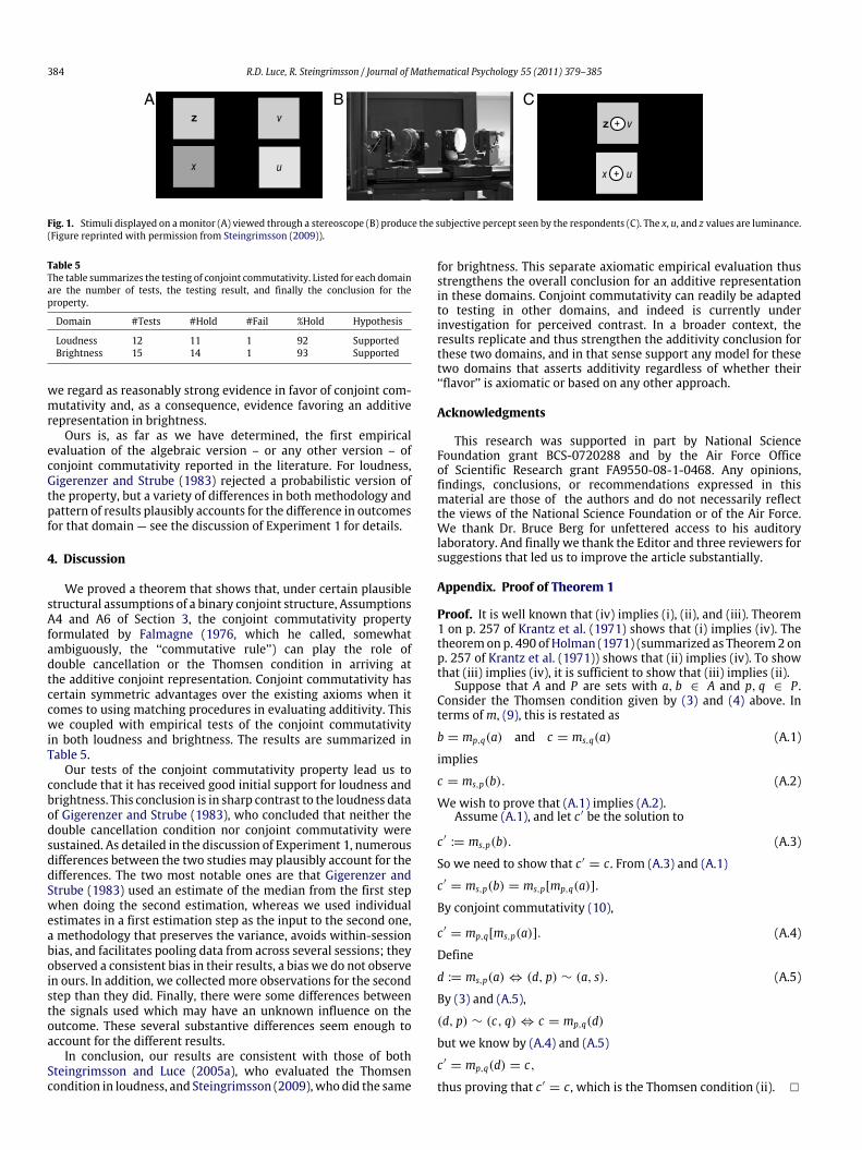
To obtain the brightness match (x, u) ∼ (z, v), the experi-menter chooses x, u, and v, and the respondent produces the zusing the method described in the Procedure section that makes(x, u) appear to be equally bright as (z, v). Fig. 1 describes the pro-cess. Panel A depicts what is displayed on the monitor, where the

letters indicate the stimulus intensity. Panel B depicts the stereo-scope through which the respondents view the monitor. Panel Cdepicts what the subject sees. Because the stereoscope creates acyclopic image, a unitary percept, these are symbolically indicatedas z ⊕ v and x ⊕ u; the symbol ⊕ stands for the unknown oper-ation that combines images in the two eyes into a single percept.The initial intensity for z is chosen at random in a 40 LUT intervalaround a best guess for its final estimate.

In terms of the stimulus display, the goal is to find the z thatwill make the percept z ⊕ v appear equally bright as the perceptx⊕u. Table 3 lists the stimulus values for the two conditions underwhich the conjoint commutativity was evaluated.

3.3.2. Results and discussionThe results are summarized in Table 4, which is organized as

Table 2.Data from two respondents were excluded for the following

reason. Our extensive experience of collectingmatching datamadeit clear that their inter-session variability was atypically large;hence we have excluded them. This should not be regarded assuspicious, because large variability generally makes it harderto reject a null hypothesis, although the M–W U test is largelyunaffected by uniform changes in variability, a feature that ishelpful in dealing statistically with inter-session variability.

The invariance property fails for one respondent in one condi-tion. This means that the property is supported in 14/15 tests. This

Table 4Results of Experiment 2: Test of the conjoint commutativity for brightness. Listed for each respondent are the conditions tested, mean (M) and standard deviations (SD) ofthe results, number of observations (n) obtained for each condition, and finally the results of the statistical testing.

Condition Respondent Intensity (cd/m2) M–W Ud SD e SD n pd∼eM M

C1 R10 207.0 11.0 209.0 8.8 30 .722C ′

1 178.3 9.87 191.5 9.5 .008C2 R22 321.4 17.8 315.0 14.1 30 .636C ′

2 275.3 18.1 261.9 19.4 .424C1 R79 163.1 16.4 159.0 18.5 30 .327C ′

1 Technical error: Data N/AC1 R81 164.7 20.5 178.6 13.4 30 .286C ′

1 160.8 15.7 154.8 16.3 .286C1 R86 157.8 18.5 153.8 16.7 51 .581C ′

1 172.3 19.1 179.8 25.0 .623C2 270 31.5 277.4 19.2 34 .922C ′

2 268.9 33.5 257.4 9.7 .418C3 R90 174.1 17.8 180.4 19.9 35 .523C ′

3 180.5 18.8 183.9 20.0 .977C3 R91 218.7 40.37 206.2 40.4 34 .525C ′

3 184 36.1 183.0 36.3 .822

384 R.D. Luce, R. Steingrimsson / Journal of Mathematical Psychology 55 (2011) 379–385

Fig. 1. Stimuli displayed on amonitor (A) viewed through a stereoscope (B) produce the subjective percept seen by the respondents (C). The x, u, and z values are luminance.(Figure reprinted with permission from Steingrimsson (2009)).

Table 5The table summarizes the testing of conjoint commutativity. Listed for each domainare the number of tests, the testing result, and finally the conclusion for theproperty.

Domain #Tests #Hold #Fail %Hold Hypothesis

Loudness 12 11 1 92 SupportedBrightness 15 14 1 93 Supported

we regard as reasonably strong evidence in favor of conjoint com-mutativity and, as a consequence, evidence favoring an additiverepresentation in brightness.

Ours is, as far as we have determined, the first empiricalevaluation of the algebraic version – or any other version – ofconjoint commutativity reported in the literature. For loudness,Gigerenzer and Strube (1983) rejected a probabilistic version ofthe property, but a variety of differences in both methodology andpattern of results plausibly accounts for the difference in outcomesfor that domain — see the discussion of Experiment 1 for details.

4. Discussion

We proved a theorem that shows that, under certain plausiblestructural assumptions of a binary conjoint structure, AssumptionsA4 and A6 of Section 3, the conjoint commutativity propertyformulated by Falmagne (1976, which he called, somewhatambiguously, the ‘‘commutative rule’’) can play the role ofdouble cancellation or the Thomsen condition in arriving atthe additive conjoint representation. Conjoint commutativity hascertain symmetric advantages over the existing axioms when itcomes to using matching procedures in evaluating additivity. Thiswe coupled with empirical tests of the conjoint commutativityin both loudness and brightness. The results are summarized inTable 5.

Our tests of the conjoint commutativity property lead us toconclude that it has received good initial support for loudness andbrightness. This conclusion is in sharp contrast to the loudness dataof Gigerenzer and Strube (1983), who concluded that neither thedouble cancellation condition nor conjoint commutativity weresustained. As detailed in the discussion of Experiment 1, numerousdifferences between the two studies may plausibly account for thedifferences. The two most notable ones are that Gigerenzer andStrube (1983) used an estimate of the median from the first stepwhen doing the second estimation, whereas we used individualestimates in a first estimation step as the input to the second one,a methodology that preserves the variance, avoids within-sessionbias, and facilitates pooling data from across several sessions; theyobserved a consistent bias in their results, a bias we do not observein ours. In addition, we collected more observations for the secondstep than they did. Finally, there were some differences betweenthe signals used which may have an unknown influence on theoutcome. These several substantive differences seem enough toaccount for the different results.

In conclusion, our results are consistent with those of bothSteingrimsson and Luce (2005a), who evaluated the Thomsencondition in loudness, and Steingrimsson (2009), who did the same

for brightness. This separate axiomatic empirical evaluation thusstrengthens the overall conclusion for an additive representationin these domains. Conjoint commutativity can readily be adaptedto testing in other domains, and indeed is currently underinvestigation for perceived contrast. In a broader context, theresults replicate and thus strengthen the additivity conclusion forthese two domains, and in that sense support any model for thesetwo domains that asserts additivity regardless of whether their‘‘flavor’’ is axiomatic or based on any other approach.

Acknowledgments

This research was supported in part by National ScienceFoundation grant BCS-0720288 and by the Air Force Officeof Scientific Research grant FA9550-08-1-0468. Any opinions,findings, conclusions, or recommendations expressed in thismaterial are those of the authors and do not necessarily reflectthe views of the National Science Foundation or of the Air Force.We thank Dr. Bruce Berg for unfettered access to his auditorylaboratory. And finally we thank the Editor and three reviewers forsuggestions that led us to improve the article substantially.

Appendix. Proof of Theorem 1

Proof. It is well known that (iv) implies (i), (ii), and (iii). Theorem1 on p. 257 of Krantz et al. (1971) shows that (i) implies (iv). Thetheoremon p. 490 of Holman (1971) (summarized as Theorem2 onp. 257 of Krantz et al. (1971)) shows that (ii) implies (iv). To showthat (iii) implies (iv), it is sufficient to show that (iii) implies (ii).

Suppose that A and P are sets with a, b ∈ A and p, q ∈ P .Consider the Thomsen condition given by (3) and (4) above. Interms ofm, (9), this is restated as

b = mp,q(a) and c = ms,q(a) (A.1)

implies

c = ms,p(b). (A.2)

We wish to prove that (A.1) implies (A.2).Assume (A.1), and let c ′ be the solution to

c ′:= ms,p(b). (A.3)

So we need to show that c ′= c. From (A.3) and (A.1)

c ′= ms,p(b) = ms,p[mp,q(a)].

By conjoint commutativity (10),

c ′= mp,q[ms,p(a)]. (A.4)

Define

d := ms,p(a) ⇔ (d, p) ∼ (a, s). (A.5)

By (3) and (A.5),

(d, p) ∼ (c, q) ⇔ c = mp,q(d)

but we know by (A.4) and (A.5)

c ′= mp,q(d) = c,

thus proving that c ′= c , which is the Thomsen condition (ii). �

R.D. Luce, R. Steingrimsson / Journal of Mathematical Psychology 55 (2011) 379–385 385

References

American Psychological Association, (2002). Ethical principles of psychologists andcode of conduct. American Psychologist , 57, 1060–1073.

Ellermeier, W., & Faulhammer, G. (2000). Empirical evaluation of axiomsfundamental to Stevens’s ratio-scaling approach: I. Loudness production.Perception and Psychophysics, 62, 1505–1511.

Ellermeier, W., Narens, L., & Dielmann, B. (2003). Perceptual ratios, differences,and the underlying scale. In B. Berglund, & E. Borg (Eds.), Fechner Day2003. Proceedings of the 19th annual meeting of the international societyfor psychophysics (pp. 71–76). Stockholm, Sweden: International Society forPsychophysics.

Falmagne, J.-C. (1976). Random conjoint measurement and loudness summation.Psychological Review, 83, 65–79.

Falmagne, J.-C., Iverson, G., & Marcovici, S. (1979). Binaural loudness summation:probabilistic theory and data. Psychological Review, 86, 25–43.

Gigerenzer, G., & Strube, G. (1983). Are there limits to binaural additivityof loudness? Journal of Experimental Psychology: Human Perception andPerformance, 9, 126–136.

Holman, E. W. (1971). A note on additive conjoint measurement. Journal ofMathematical Psychology, 8, 489–494.

Krantz, D. H., Luce, R. D., Suppes, P., & Tversky, A. (1971–2007). Foundations ofmeasurement, Vol. I. Academic Press, Reprinted 2007 by Dover Publications.

Legge, G. E., & Rubin, G. S. (1981). Binocular interactions in suprathreshold contrastperception. Perception & Psychophysics, 30, 49–61.

Levelt,W. J. M., Riemersma, J. B., & Bunt, A. A. (1972). Binaural additivity of loudness.British Journal of Mathematical and Statistical Psychology, 25, 51–68.

Luce, R. D. (1995). Four tensions concerning mathematical modeling in psychology.Annual Reviews of Psychology, 46, 1–26.

Luce, R. D. (2004). Symmetric and asymmetric matching of joint presentations.Psychological Review, 111, 446–454.

Luce, R. D. (2008). Correction to Luce (2004). Psychological Review, 115, 601.Luce, R. D., Krantz, D. H., Suppes, P., & Tversky, A. (1990–2007). Foundations of

measurement, Vol. III. Academic Press, Reprinted 2007 by Dover Publications.Luce, R. D., Steingrimsson, R., & Narens, L. (2010). Are psychophysical scales of

intensities the same or different when stimuli vary on other dimensions?Theory with experiments varying loudness and pitch. Psychological Review, 117,1247–1258.

Luce, R. D., & Tukey, J. (1964). Simultaneous conjoint measurement: a new type offundamental measurement. Journal of Mathematical Psychology, 1, 1–27.

Schneider, B. (1988). The additivity of loudness across critical bands: a conjointmeasurement approach. Perception & Psychophysics, 43, 211–222.

Steingrimsson, R. (2009). Evaluating amodel of global psychophysical judgments inbrightness: I. Behavioral properties of summations and productions. Attention,Perception & Psychophysics, 71, 1916–1930.

Steingrimsson, R. (2011). Evaluating a model of global psychophysical judgmentsfor brightness: II. Behavioral Properties Linking Summations and Productions.Attention, Perception & Psychophysics, 73, 872–885. doi:10.3758/s13414-010-0067-5.

Steingrimsson, R., & Luce, R. D. (2005a). Evaluating amodel of global psychophysicaljudgments: I. Behavioral properties of summations and productions. Journal ofMathematical Psychology, 49, 290–307.

Steingrimsson, R., & Luce, R. D. (2005b). Evaluating amodel of global psychophysicaljudgments: II. Behavioral properties linking summations and productions.Journal of Mathematical Psychology, 49, 308–319.

Steingrimsson, R., & Luce, R. D. (2006). Empirical evaluation of a model of globalpsychophysical judgments: III. A form for the psychophysical function andintensity filtering. Journal of Mathematical Psychology, 50, 15–29.

Steingrimsson, R., & Luce, R. D. (2007). Empirical evaluation of a model of globalpsychophysical judgments: IV. Forms for the weighting function. Journal ofMathematical Psychology, 51, 29–44.

Steingrimsson, R., & Luce, R. D. (2010). The commutative rule as new test for additiveconjoint measurement: theory and data. In A. Bastianelli, & G. Vidotto (Eds.),Fechner day 2010. Proceedings of the 19th annual meeting of the internationalsociety for psychophysics (pp. 21–26). Padua, Italy: International Society forPsychophysics.

Suppes, P., Krantz, D. H., Luce, R. D., & Tversky, A. (1989–2007). Foundations ofmeasurement, Vol. II. Academic Press, Reprinted 2007 by Dover Publications.

Ward, L. M. (1990). Cross-modal additive conjoint structures and psychophysicalscale convergence. Journal of Experimental Psychology: General, 119, 161–175.

Zimmer, K., Luce, R.D., & Ellermeier, W. (2001). Testing a new theory ofpsychophysical scaling: Temporal loudness integration. In G. Sommerfeld, R.Kompass and T. Lachmann (eds.), Fechner day 2001, Proceedings of the 17thannual meeting of the international society for psychophysics.

Zimmer, K. (2005). Examining the validity of numerical ratios in loudnessfractionation. Perception & Psychophysics, 67, 569–579.