the vp/vs relationship of the basement under the trøndelag
TRANSCRIPT
Master Thesis, Department of Geosciences
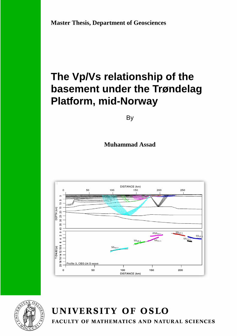
The Vp/Vs relationship of the basement under the Trøndelag Platform, mid-Norway
By
Muhammad Assad
The Vp/Vs relationship of the basement under the Trøndelag Platform, mid-Norway
By
Muhammad Assad
Master Thesis in Geosciences
Discipline: Geophysics
Department of Geosciences
Faculty of Mathematics and Natural Sciences
University of Oslo (June 2013)

© Muhammad Assad, 2013
Tutors(s): Asbjørn Breivik, Jan Inge Faleide and Abhishek Kumar Rai
This work is published digitally through DUO – Digitale Utgivelser ved UiO
http://www.duo.uio.no
It is also catalogued in BIBSYS (http://www.bibsys.no/english)
All rights reserved. No part of this publication may be reproduced or transmitted, in any form or by any means,
without permission.

Acknowledgement
I would like to express my gratitude to my supervisors Asbjørn Breivik (UiO), Jan Inge Faleide (UiO) and Abhishek Kumar Rai (UiO) for their support and encouragement throughout my thesis work. I am very grateful to them for their advices and feedbacks on my work. I also thankful to University of Oslo and Bergen University for providing me the data and resources necessary to carry on this work. Finally, my special thanks to my family for their support and patience, not only during this work, but also during the last years.
1
TABLE OF CONTENTS Page No Abstract 1
1) Introduction 2
2.1) Development of Mid-Norway Continental Margin 5
2.2) Structural and tectonic elements of Norwegian Continental Margin 9
3.1 Seismic Waves 14
• 3.1.1 P-Waves 1 4
• 3.1.2 S-Waves 15
• 3.1.3 S-wave Splitting 16
3.2 Ray Theory 17
• 3.2.1 Snell’s Law and Wave Conversions 18
• 3.2.2Theoretical Partitioning of Seismic Energy at crust-Mohorovivic interface 18
• 3.2.3 Theoretical Partitioning of Seismic Energy at ocean bottom 22
3.3 Poisson Ratio 23
4.1 Forward Seismic Modeling Methodologies 25
• 4.1.1 Introduction 25
• 4.1.2 Identification of Arrivals/Signals 25
• 4.1.3 Certainty of the Interpretation/Picks 29
• 4.1.4 Reciprocity of Travel times 29
4.2 Modeling Strategy 29
• 4.2.1 Programmed Ray Tracing 31
• 4.2.2 Ray Search Mode 34
5 Processing of wide-angle seismic data 37
• 5.1 Velocity Reduction 36
• 5.2 Band pass filtering 39
• 5.3 Spiking Deconvolution 41
• 5.4 Automatic Gain Control (AGC) 43
• 5.5 Rotation of Data relative to source-receiver plane 45
6 Interpretation and Modeling of Data 47
• 6.1Classification of s-wave arrivals 48
• 6.2 Interpretation and Modeling of Profile3-03 49
• 6.3 Interpretation and Modeling of Profile4-03 53
2
• 6.4 Interpretational Uncertainties 56
• 6.5 Conversion Efficiency and Statistics 57
• 6.6 Modeling Results 58
7 Discussion on Results 61
• 7.1 Vp/Vs ratio for sediments 61
• 7.2 Vp/Vs for Basement and Mantle 63
• 7.3 Lithological Interpretation 64
8 Conclusions 67
References 68
Appendix 75
1
Abstract
Two wide angle 3-Compnent Ocean Bottom Seismometer (OBS) profiles along with
associated Land-Stations acquired during 2003 under the EUROMARGINS Program were
analyzed during this M.Sc. Thesis. These profiles are named as PROFILE -3-03 & 4-03 &
were aimed at studying the crustal structure beneath the Trøndelag Platform & adjacent areas,
mid-Norway. Shear waves recorded on the horizontal components of the seismometers have
been modeled using 2-D kinematic ray-tracing software RAYINVR, utilizing already
generated p-wave velocity models. For shallower sediments (1-6 km depths) average Vp/Vs
ratios are relatively high as expected i.e. 2.0-2.6 which indicate the presence of low
consolidated sediments in the upper layers. The deeper sedimentary layers (6-11 km depth)
present along NW side of both profiles exhibit lower Vp/Vs ratios i.e. 1.8-2.0 which represent
further compacted sediments because of increased burial. The upper crust has an average
Vp/Vs ratio in the range 1.75-1.78 which suggests that the crust under the Trøndelag Platform
is felsic. Vp/Vs ratio increases to 1.80-1.85 in the lower crust which suggests the presence of
mafic to ultra-mafic lower crust.
2
1) Introduction
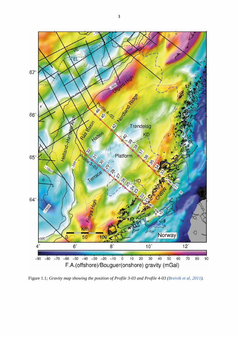
The sedimentary cover underneath Trøndelag Platform and Halten Terrace is well-known
because of detailed coverage of commercial seismic reflection surveys and subsequent well
data carried out for HC exploration. However, less information is available about the deeper
structures in this area. Therefore, in order to map deeper crust two Ocean Bottom Seismic
(OBS) profiles (Profile 3-03 and Profile 4-03) were acquired in 2003 by Håkon Mosby under
the Euro Margins Program. These included OBS stations and associated land stations. The
study area is shown in figure 1.1 (Breivik et al, 2011).
Profile 3-03 has data from twelve OBS’s (ocean bottom seismometers) and five land stations
and has a length of 285 km continuing in the NW-SE direction. Whereas Profile 4-03 extends
up to 356 km’s and includes data from eleven OBS’s and six land stations, having nearly the
same orientation as Profile 3-03. Expect few OBH stations (Ocean Bottom Hydrophones),
which record seismic signal in vertical direction only, all the other instruments were capable
of recording seismic signal in vertical and two horizontal directions as well.
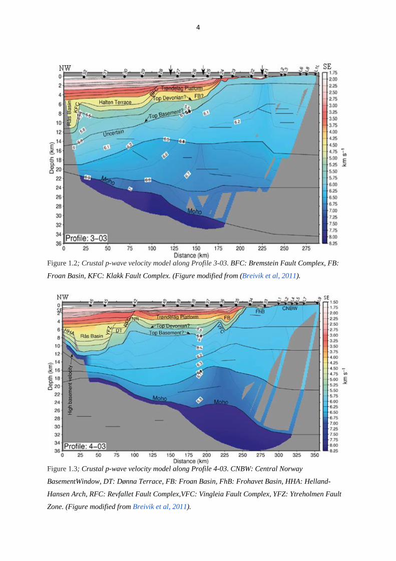
The p-wave velocity modeling has already been carried out using the vertical component of 3-
C Geophones and wide angle OBS Stations data for both profiles. P-wave modeling shows
continental crust deep under both the profiles. It reveals that basement is composed of
distinctive velocity layers and its thickness increases from NW to SE as shown in figure 1.2
and 1.3 (Breivik et al, 2011).
The purpose of this thesis is to obtain the s-wave velocity values for different parts of the
already generated p-wave models using the information from arrivals at the horizontal
components of the OBS and Land Stations. It will enable mapping of Vp/Vs ratios along the
profiles. The Vp/Vs ratios will be used to discuss velocity differences i.e. possible lithology
indications and basement rock composition for the different parts of the models.
In order to achieve the above objective first the wide angle OBS data will be processed using
Seismic Unix software. It will be followed by interpretation of different s-wave arrivals on
horizontal components of OBS’s on both profiles. Third step will be the modeling of s-wave
arrivals using RAYINVR software. It will be carried out using already generated p-wave
velocity models as basis for s-wave velocity modeling.
Finally, the modeling results will provide ratios for p and s-wave velocities i.e. Vp/Vs ratios
for different parts of the p-wave velocity models which will be discussed in the last section.
3
Figure 1.1; Gravity map showing the position of Profile 3-03 and Profile 4-03 (Breivik et al, 2011).
4
Figure 1.2; Crustal p-wave velocity model along Profile 3-03. BFC: Bremstein Fault Complex, FB:
Froan Basin, KFC: Klakk Fault Complex. (Figure modified from (Breivik et al, 2011).
Figure 1.3; Crustal p-wave velocity model along Profile 4-03. CNBW: Central Norway
BasementWindow, DT: Dønna Terrace, FB: Froan Basin, FhB: Frohavet Basin, HHA: Helland-
Hansen Arch, RFC: Revfallet Fault Complex,VFC: Vingleia Fault Complex, YFZ: Ytreholmen Fault
Zone. (Figure modified from Breivik et al, 2011).
5
2.1) Development of Mid-Norway Continental Margin
Mid-Norway continental margin evolved differently as compared to other Passive continental
margins as it experienced prolonged rifting episode and significant tectonic activity continued
even after crustal separation (Bukovics and Ziegler, 1984, Smelror et al., 2007).
2.1.1) Basinal Development during Palaeozoic;
Caledonian Orogeny was a result of collision between Greenland-Laurentian Plate and
Fennoscandian-Russian Plate in Ordovician to Early Devonian Times. From Early Devonian
onwards the Caledonides formed during Caledonian Orogeny started to collapse due to the
diminishing thrusting activity (Andersen et al, 1991; Milnes et al. 1997; Fossen, 2000; Terry
et al. 2000).
Regional crustal extension dominated the evolution of Norwegian-Greenland Sea from Late
Carboniferous onwards. Development of rift system resulted in accumulation of Permian
carbonates and clastics into the large half-grabens (Haller, 1971). Similarly, a rapid
subsidence of the eastern part of Trøndelag Platform was observed during the Late Paleozoic
(Blystad et al., 1995, Bukovics and Ziegler, 1984, Smelror et al., 2007).
This extension activity continued until Late Permian times. It resulted in the transgression of
Arctic Permian seas into the Northern and Southern Permian basins of the Northwest Europe.
This transgression was facilitated by Norwegian-Greenland Sea Rift system (Smelror et al.,
2007, Ziegler, 1982).
2.1.2) First rifting stage in Early Mesozoic;
Crustal extension in Norwegian-Greenland sea area paced up during the Early Triassic times.
Rifting continued to extend southward to the North Sea area (Ziegler, 1982). Triassic strata
deposited on Trøndelag Platform show the evidence of subsidence and rifting as it has
developed syn-depositional tensional faulting (Blystad et al., 1995, Bukovics and Ziegler,
1984, Smelror et al., 2007).
Almost entire Mid-Norway shelf was affected by the Triassic-Jurassic rifting stages (Phase 1
as shown in Figure 2.1). Trøndelag Platform is more intensely faulted on the western side than
the eastern one. Fault rotation and their geometries suggest that mechanical stretching and
associated thinning are the most obvious cause of subsidence of Norwegian-Greenland Sea
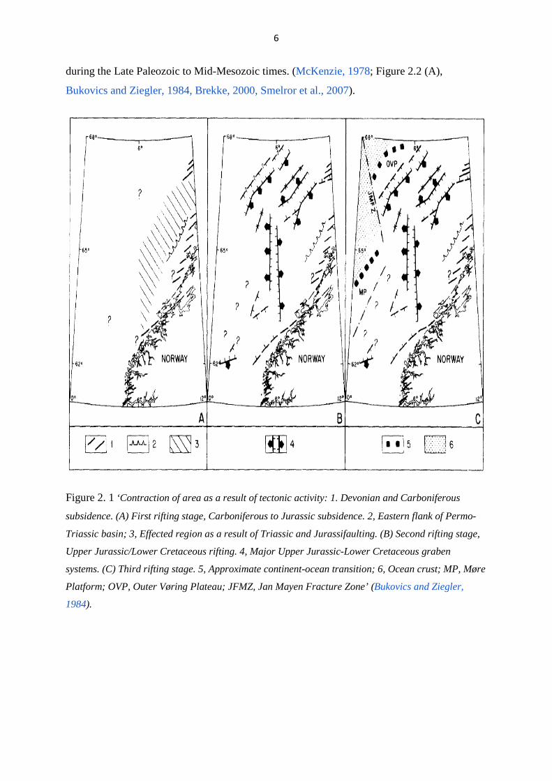
6
during the Late Paleozoic to Mid-Mesozoic times. (McKenzie, 1978; Figure 2.2 (A),
Bukovics and Ziegler, 1984, Brekke, 2000, Smelror et al., 2007).
Figure 2. 1 ‘Contraction of area as a result of tectonic activity: 1. Devonian and Carboniferous
subsidence. (A) First rifting stage, Carboniferous to Jurassic subsidence. 2, Eastern flank of Permo-
Triassic basin; 3, Effected region as a result of Triassic and Jurassifaulting. (B) Second rifting stage,
Upper Jurassic/Lower Cretaceous rifting. 4, Major Upper Jurassic-Lower Cretaceous graben
systems. (C) Third rifting stage. 5, Approximate continent-ocean transition; 6, Ocean crust; MP, Møre
Platform; OVP, Outer Vøring Plateau; JFMZ, Jan Mayen Fracture Zone’ (Bukovics and Ziegler,
1984).
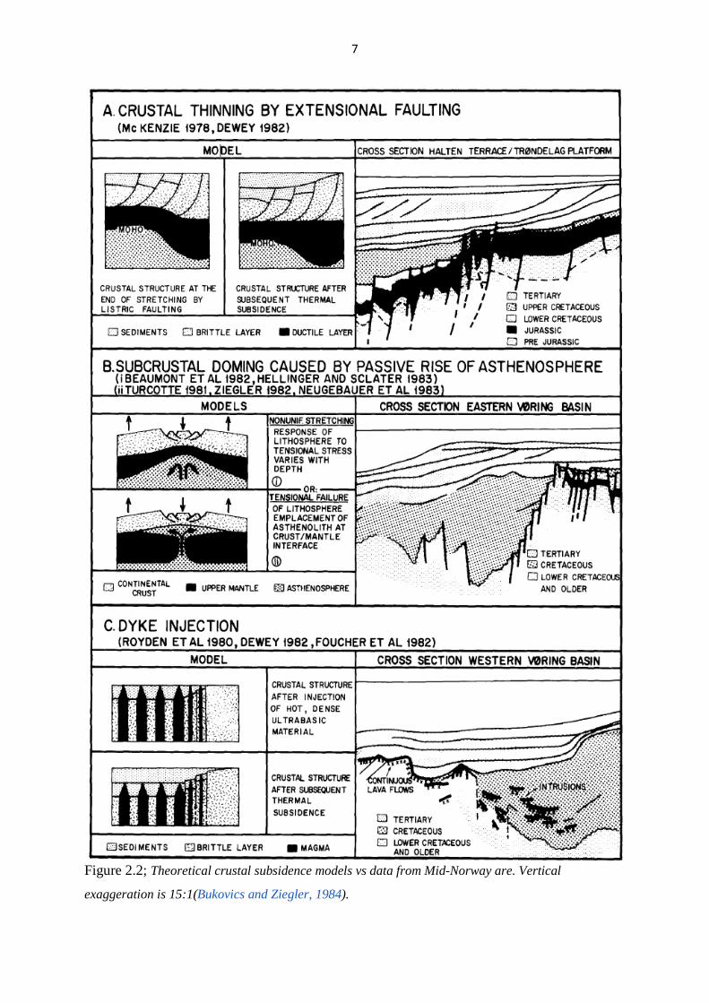
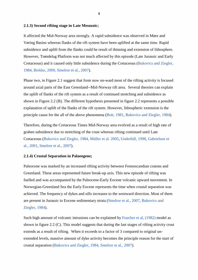
7
Figure 2.2; Theoretical crustal subsidence models vs data from Mid-Norway are. Vertical
exaggeration is 15:1(Bukovics and Ziegler, 1984).
8
2.1.3) Second rifting stage in Late Mesozoic;
It affected the Mid-Norway area strongly. A rapid subsidence was observed in Møre and
Vøring Basins whereas flanks of the rift system have been uplifted at the same time. Rapid
subsidence and uplift from the flanks could be result of thinning and extension of lithosphere.
However, Trøndelag Platform was not much affected by this episode (Late Jurassic and Early
Cretaceous) and it caused only little subsidence during the Cretaceous (Bukovics and Ziegler,
1984, Brekke, 2000, Smelror et al., 2007).
Phase two, in Figure 2.1 suggest that from now on-ward most of the rifting activity is focused
around axial parts of the East Greenland--Mid-Norway rift area. Several theories can explain
the uplift of flanks of the rift system as a result of continued stretching and subsidence as
shown in Figure 2.2 (B). The different hypothesis presented in figure 2.2 represents a possible
explanation of uplift of the flanks of the rift system. However, lithospheric extension is the
principle cause for the all of the above phenomena (Bott, 1981, Bukovics and Ziegler, 1984).
Therefore, during the Cretaceous Times Mid-Norway area evolved as a result of high rate of
graben subsidence due to stretching of the crust whereas rifting continued until Late
Cretaceous (Bukovics and Ziegler, 1984, Müller et al. 2005, Underhill, 1998, Gabrielsen et
al., 2001, Smelror et al., 2007).
2.1.4) Crustal Separation in Palaeogene;
Paleocene was marked by an increased rifting activity between Fennoscandian cratons and
Greenland. These areas represented future break-up axis. This new episode of rifting was
fuelled and was accompanied by the Paleocene-Early Eocene volcanic upward movement. In
Norwegian-Greenland Sea the Early Eocene represents the time when crustal separation was
achieved. The frequency of dykes and sills increases to the westward direction. Most of them
are present in Jurassic to Eocene sedimentary strata (Smelror et al., 2007, Bukovics and
Ziegler, 1984).
Such high amount of volcanic intrusions can be explained by Foucher et al, (1982) model as
shown in figure 2.2 (C). This model suggests that during the last stages of rifting activity crust
extends as a result of rifting. When it exceeds to a factor of 3 compared to original un-
extended levels, massive amount of dyke activity becomes the principle reason for the start of
crustal separation (Bukovics and Ziegler, 1984, Smelror et al., 2007).
9
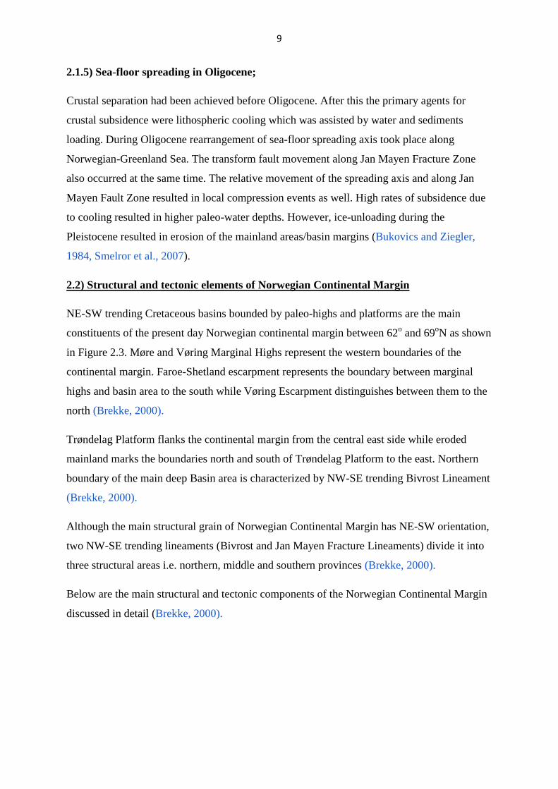
2.1.5) Sea-floor spreading in Oligocene;
Crustal separation had been achieved before Oligocene. After this the primary agents for
crustal subsidence were lithospheric cooling which was assisted by water and sediments
loading. During Oligocene rearrangement of sea-floor spreading axis took place along
Norwegian-Greenland Sea. The transform fault movement along Jan Mayen Fracture Zone
also occurred at the same time. The relative movement of the spreading axis and along Jan
Mayen Fault Zone resulted in local compression events as well. High rates of subsidence due
to cooling resulted in higher paleo-water depths. However, ice-unloading during the
Pleistocene resulted in erosion of the mainland areas/basin margins (Bukovics and Ziegler,
1984, Smelror et al., 2007).
2.2) Structural and tectonic elements of Norwegian Continental Margin
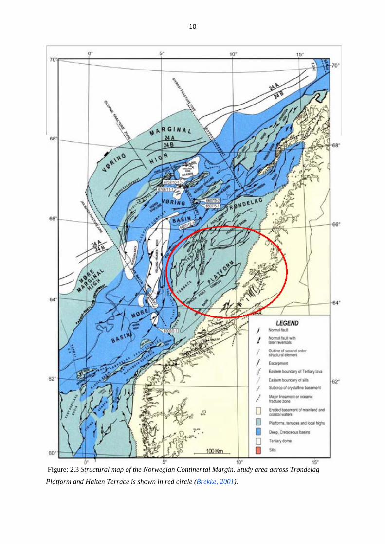
NE-SW trending Cretaceous basins bounded by paleo-highs and platforms are the main
constituents of the present day Norwegian continental margin between 62o and 69oN as shown
in Figure 2.3. Møre and Vøring Marginal Highs represent the western boundaries of the
continental margin. Faroe-Shetland escarpment represents the boundary between marginal
highs and basin area to the south while Vøring Escarpment distinguishes between them to the
north (Brekke, 2000).
Trøndelag Platform flanks the continental margin from the central east side while eroded
mainland marks the boundaries north and south of Trøndelag Platform to the east. Northern
boundary of the main deep Basin area is characterized by NW-SE trending Bivrost Lineament
(Brekke, 2000).
Although the main structural grain of Norwegian Continental Margin has NE-SW orientation,
two NW-SE trending lineaments (Bivrost and Jan Mayen Fracture Lineaments) divide it into
three structural areas i.e. northern, middle and southern provinces (Brekke, 2000).
Below are the main structural and tectonic components of the Norwegian Continental Margin
discussed in detail (Brekke, 2000).
10
Figure: 2.3 Structural map of the Norwegian Continental Margin. Study area across Trøndelag
Platform and Halten Terrace is shown in red circle (Brekke, 2001).
11
2.2.1) Jan Mayen Lineament
It represents the boundary between the Møre Basin to the south and the Vøring Basin to the
north. It can be distinguished by counter clockwise shift of basinal flanks and axes. It also
marks the boundary of the Trøndelag Platform to the south (Brekke, 2000).
2.2.2) Bivrost Lineament
It distinguishes the Vøring Basin from the uplifted continental margin around Loften to the
north. It matches with the Trøndelag Platform termination to the north. It can also be
distinguished as a clock wise shift in basinal axes and associated flanked portions (Blystad et
al, 1995; Brekke, 2000).
2.2.3) Vøring Basin
It encompasses areas between 64-68°N and 2-10°E and is a large basin having grabens, sub-
basins and structural highs as salient features. The distinguishing feature of Vøring Basin is
the enormous thickness of Cretaceous sequence. In some parts, the cretaceous base is as much
as 9s twt (two way travel time) deep in the seismic section (Bukovics and Ziegler, 1985;
Blystad et al, 1995).
Vøring Basin is bordered by the Vøring Escarpment from the west and is bounded by fault
complexes around the corners of Trøndelag Platform in the eastward direction. Fles Fault
Complex bisects the basin and runs parallel to basin axes from Jan Mayen Lineament to
Bivrost Lineament. It also has Paleocene mafic intrusions as sills. Most of the sills are present
in the western part and seismic reflections coming from underlying strata below the sills are
blurred. Magmatic activity was the result of continental breakup (Bukovics et al, 1984;
Blystad et al, 1995; Brekke, 2000, Eldholm and Coffin, 2000; Eldholm and Grue, 1994).
Helland Hansen Arch is the most prominent structural high in the Vøring Basin present in
central southern part. It was formed as a result of compressional tectonics in the Cenozoic era
by the reverse reactivations of the Fles Fault Complex. Surt Lineament which also includes
the Rym Fault Zones separates the northern part of the basin (Brekke, 2000).
2.2.4) Vøring Marginal High and Møre Basin
It is situated between Jan Mayen and Bivrost Lineaments and to the west of Vøring
Escarpment. It is composed of Tertiary deposits overlying the continental crust. The
12
continental crust gets thinner and changes to oceanic crust in the westward direction (Blystad
et al., 1995; Brekke, 2000). The boundary of Møre Basin is marked by Faeroe-Shetland
Escarpment from the west, Møre-Trøndelag Fault Complex to the southwest and by Jan
Mayen Lineament from the north. Its structural elements have NE-SW trend consisting of
highs, ridges and smaller basins and it is about 9s twt (two way travel time) thick from the
axial part. Its main tectonic episode was in Mid-Jurassito Early-Cretaceous rifting and was
formed by the subsidence of its flanks as a result of rifting (Brekke, 2000).
2.2.6) Møre-Trøndelag Fault Complex
It comprises the south eastern margin of Møre Basin and consists of NE-SW trending fault-
controlled ridges and smaller scale basins. Its trend follow the dominant orientation of
structures formed during Caledonian deformation and has been subject to reactivation various
times in geological record. As a result it has affected the Paleozoic, Devonian, Jurassic age
rocks and Precambrian basement (Bering 1992; Grønlie et al., 1994; Brekke, 2000; Blystad et
al., 1995).
2.2.7) Trøndelag Platform
As shown in the structural map Trøndelag Platform, Vøring Basin and the Vøring Marginal
High are the middle structural provinces bounded by Jan Mayen and Bivrost Lineaments.
Trøndelag Platform is present between Vøring Basin and Norwegian mainland and is about
160 km. Wide horst and half-grabens present in the inner portions of Trøndelag Platform are
characterized by tectonic activity which took place in Carboniferous to Late Permain times
(Brekke, 2000).
However, continued activation of some major extensional faults until the Triassic age resulted
in en-echelon NE-SW trending basins like Froan Basin, which were filled by Triassic to early
Paleozoic sediments and lies southwards (Brekke, 2000).
Froan Basin is separated from inner parts of Trøndelag Platform in NW direction by Vingelia
Fault Complex which shows signs of reactivation in both Jurassic and Cretaceous ages. From
NW to SE-direction Froan Basin fill becomes progressively thin/shallower. This thinning is
attributed to two factors. First, natural thinning of basin fill to the landward direction coupled
with erosion and uplifting during mid to Late Jurassic (Brekke, 2000).
13
Interior parts of the Trøndelag Platform experienced small scale faulting in mid-Jurassic to
Early-Cretaceous partly by faulting along the flanks of Helgeland Basin and reactivations of
faults present in Vingleia Fault Complex. The same tectonic phase produced intense faulting
in Dønna and Halten Terraces. It also resulted in initiation of subdivision in the deep basin on
western side was also started during the same tectonic stage (Brekke, 2000).
However, Halten Terrace and Trøndelag Platform had the same elevation until Early-
Cretaceous tectonic activity. Thus Nordland Ridge and Froya high present on the edge of
Trøndelag Platform had the same elevation levels as the Sklinna until Early-Cretaceous
(Brekke, 2000).
14
3.1) Seismic Waves;
Seismic waves are a form of energy. These are caused by a sudden disturbance of the rock in
earth. The source of disturbance could be natural i.e. earthquakes or man-made i.e. dynamite
etc. These travel through the earth and are recorded at recording stations.
There is different kind of seismic waves depending upon the nature of their motion. However
two most important categories are surface and body waves. Body waves can penetrate the
earth while surface waves can only propagate into the shallow earth i.e. close to the surface.
Therefore, body wave’s propagation is used to study the earth’s interior. As this thesis deals
with ray-tracing and modeling of body waves, so only these will be discussed in detail.
There are two types of body waves, P and S-waves.
3.1.1) P-Waves;
P or primary waves are the fastest travelling waves and are first to reach a seismic station.
These are also called pressure waves as they travel in the form of compressions and
rarefactions. P-waves can travel through both liquids and solids. The wave’s propagation
direction is in the same direction as the particles motion direction.
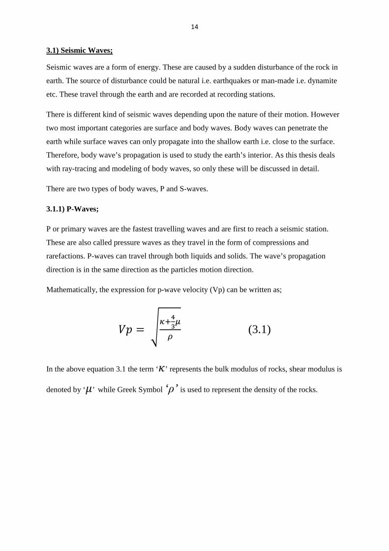
Mathematically, the expression for p-wave velocity (Vp) can be written as;
𝑉𝑝 = �𝜅+43𝜇
𝜌 (3.1)
In the above equation 3.1 the term ‘𝜅’ represents the bulk modulus of rocks, shear modulus is
denoted by ‘𝜇’ while Greek Symbol ‘ρ’ is used to represent the density of the rocks.
15
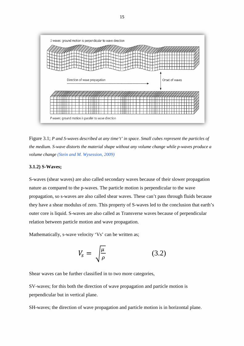
Figure 3.1; P and S-waves described at any time‘t’ in space. Small cubes represent the particles of
the medium. S-wave distorts the material shape without any volume change while p-waves produce a
volume change (Stein and M. Wysession, 2009)
3.1.2) S-Waves;
S-waves (shear waves) are also called secondary waves because of their slower propagation
nature as compared to the p-waves. The particle motion is perpendicular to the wave
propagation, so s-waves are also called shear waves. These can’t pass through fluids because
they have a shear modulus of zero. This property of S-waves led to the conclusion that earth’s
outer core is liquid. S-waves are also called as Transverse waves because of perpendicular
relation between particle motion and wave propagation.
Mathematically, s-wave velocity ‘Vs’ can be written as;
𝑉𝑠 = �𝜇 𝜌
(3.2)
Shear waves can be further classified in to two more categories,
SV-waves; for this both the direction of wave propagation and particle motion is
perpendicular but in vertical plane.
SH-waves; the direction of wave propagation and particle motion is in horizontal plane.
16
3.1.3 S-wave Splitting;
Any material which has the same physical properties in all the directions is called isotropic.
While anisotropy is the result of material’s different physical properties in different directions,
called heterogeneity.
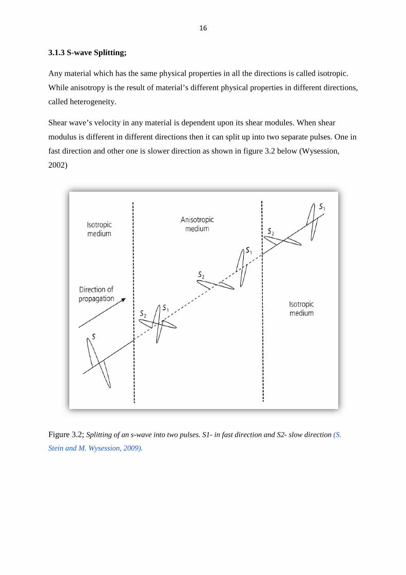
Shear wave’s velocity in any material is dependent upon its shear modules. When shear
modulus is different in different directions then it can split up into two separate pulses. One in
fast direction and other one is slower direction as shown in figure 3.2 below (Wysession,
2002)
Figure 3.2; Splitting of an s-wave into two pulses. S1- in fast direction and S2- slow direction (S.
Stein and M. Wysession, 2009).
17
3.2) Ray Theory;
Rays are defined as normal to a propagating wave front and point in the direction of the
propagation of wave field. It is a high frequency approximation of the wave theory. Therefore,
for it to hold the change in the medium physical parameters i.e. P and S velocities should not
be much as compared the length of the dominant wavelength (Daley and Krebes, 2004).
If above conditions are met, then the propagating wave’s travel time T(x) for the source of
seismic energy to a subsurface point x = (x, y, z) in an isotropic and heterogeneous medium
that follows the Eikonal Equation (Daley and Krebes, 2004).
i.e.
(∇T)2= �𝜕𝑇𝜕𝑥�2
+ �𝜕𝑇𝜕𝑦�2
+ �𝜕𝑇𝜕𝑧�2
= 1𝑣2
(3.3)
Where v=v(x) is the velocity of the seismic wave.
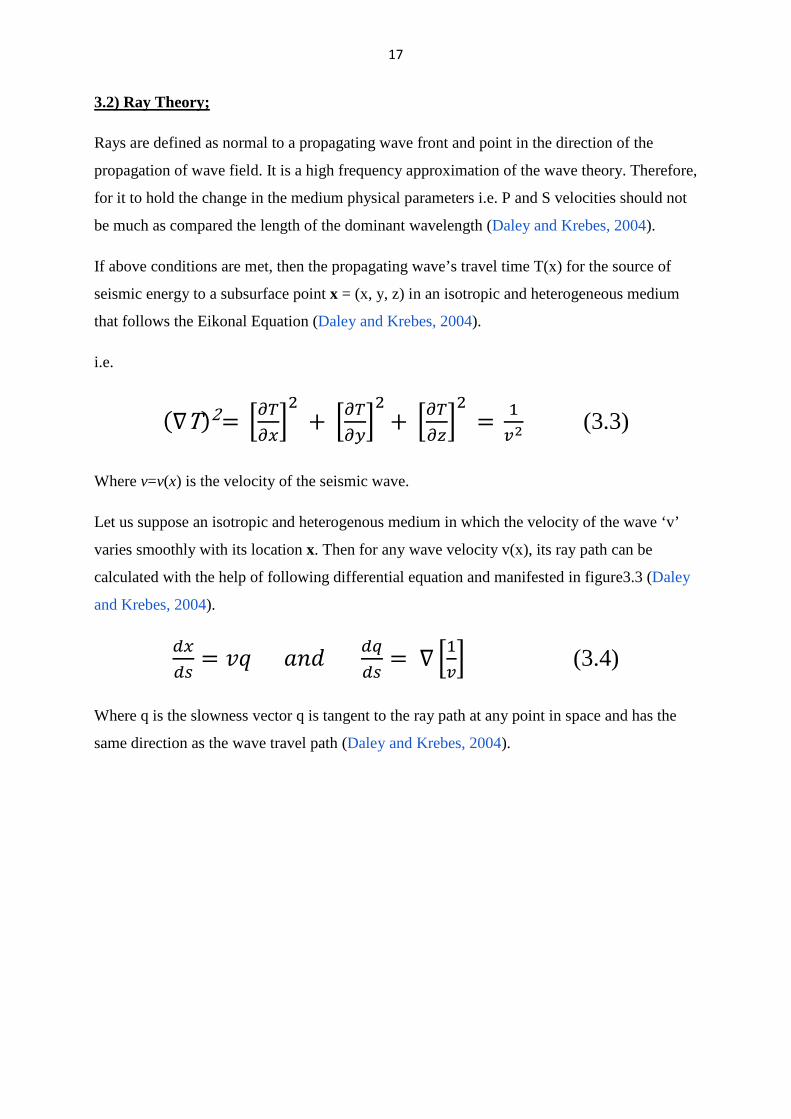
Let us suppose an isotropic and heterogenous medium in which the velocity of the wave ‘v’
varies smoothly with its location x. Then for any wave velocity v(x), its ray path can be
calculated with the help of following differential equation and manifested in figure3.3 (Daley
and Krebes, 2004).
𝑑𝑥𝑑𝑠
= 𝑣𝑞 𝑎𝑛𝑑 𝑑𝑞𝑑𝑠
= ∇ �1𝑣� (3.4)
Where q is the slowness vector q is tangent to the ray path at any point in space and has the
same direction as the wave travel path (Daley and Krebes, 2004).
18
Figure 3.3: Ray path in a vertically heterogeneous half space in which wave velocity varies with
depth z as v=exp (z2). Ray has a 5.74o take-off angle with a travel time of 1.79 s (Daley and Krebes,
2004).
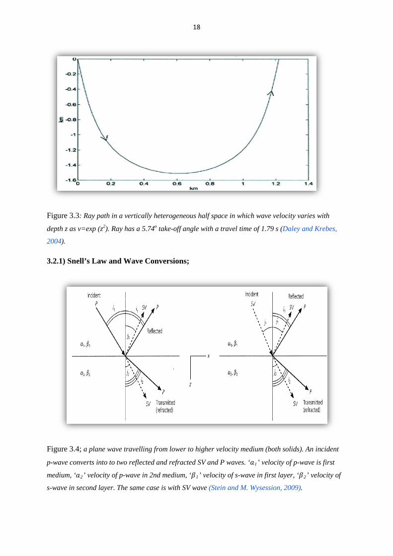
3.2.1) Snell’s Law and Wave Conversions;
Figure 3.4; a plane wave travelling from lower to higher velocity medium (both solids). An incident
p-wave converts into to two reflected and refracted SV and P waves. ‘𝑎R1’ velocity of p-wave is first
medium, ‘𝑎R2’ velocity of p-wave in 2nd medium, ‘𝛽R1’ velocity of s-wave in first layer, ‘𝛽R2’ velocity of
s-wave in second layer. The same case is with SV wave (Stein and M. Wysession, 2009).
19
Snell’s law represents a mathematical explanation of any physical change in the direction of
any wave-front when it impinges upon a lithological layer having some acoustic impedance
contrast (z=velocity of wave × density of the material) and the conversion of the p or s-wave
at the boundary of the media. Change in the direction of wave-front may include refraction or
reflection (E.S. Robinson and C. Çoruh, 1988).
Mathematically, it is written as,
𝑐𝑥 = 𝛼1𝑠𝑖𝑛𝑖1
= 𝛽1𝑠𝑖𝑛𝑗1
= 𝛼2𝑠𝑖𝑛𝑖2
= 𝛽2𝑠𝑖𝑛𝑗2
(3.5)
Where cx is the apparent velocity of the wave (S. Stein and M. Wysession, 2009).
As shown in figure; 3.4, the incident p-wave is inclined to the interface. It means it has both
longitudinal and transverse sense of particle motion; therefore, both p and s-waves are
generated. The change in direction of the refracted p and s-waves is related to the acoustic
contrast between the two media. The greater the contrast more will be the deviation of
refracted rays from the normal (S. Stein and M. Wysession, 2009).
Since as the Snell’s law requires that apparent velocity ‘cx’ of all generated waves at an
interface to be the same, S-waves are closer to the normal than the p-waves, because they
travel at lesser speeds in any medium as compared to p-waves. In case of more interfaces,
since all the generated waves satisfy Snell’s law and have same ray parameter ‘p’, so a ray
can be traced (S. Stein and M. Wysession, 2009).
3.2.2) Theoretical Partitioning of Seismic Energy at crust-Mohorovicic interface;
As it has been shown in figure 3.4 above that when an inclined p-wave ray is incident on an
acoustic interface, it gets converted into reflected and refracted P and SV-waves. At a
boundary the tangential and normal components of the displacement must be continuous (S.
Stein and M. Wysession, 2009).
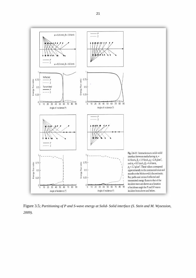
The figures 3.5 show various theoretical cases of p and s-waves incident upon Mohorovicic
discontinuity (S. Stein and M. Wysession, 2009).
At this discontinuity four different waves are generated and according to law of conservation
of energy, the sum of all of their energies must be equal to 1.
20
For an incident p-wave most of the energy (97%) is transmitted as p-wave for angles of
incidence less than the critical angle i.e. 58º as shown in the figure 3.5. After the critical
angle, the ratio of reflected p-wave energy increases to about 90%, however, this time the
ratio of converted s-waves (both reflected and refracted) increases up to 10%. For a p-wave
incident from below the equation remains almost the same except there is no critical angle as
the wave enters from higher to lower velocity layer. It should be noted that at zero incidence
angle, whole of the p-wave is transmitted (S. Stein and M. Wysession, 2009).
Similarly, for an SV-wave almost 99% of the energy is transmitted as s-wave at the zero angle
of incidence while about 1% is reflected as sv-wave and no p-wave is generated. After 20o of
incidence, the pattern starts to change slowly, and the strength of reflected SV-wave energy
increases on the strength of transmitted energy until the critical angle (58o) reaches. After it,
SV-wave energy vanishes (S. Stein and M. Wysession, 2009).
21
Figure 3.5; Partitioning of P and S-wave energy at Solid- Solid interface (S. Stein and M. Wysession,
2009).
22
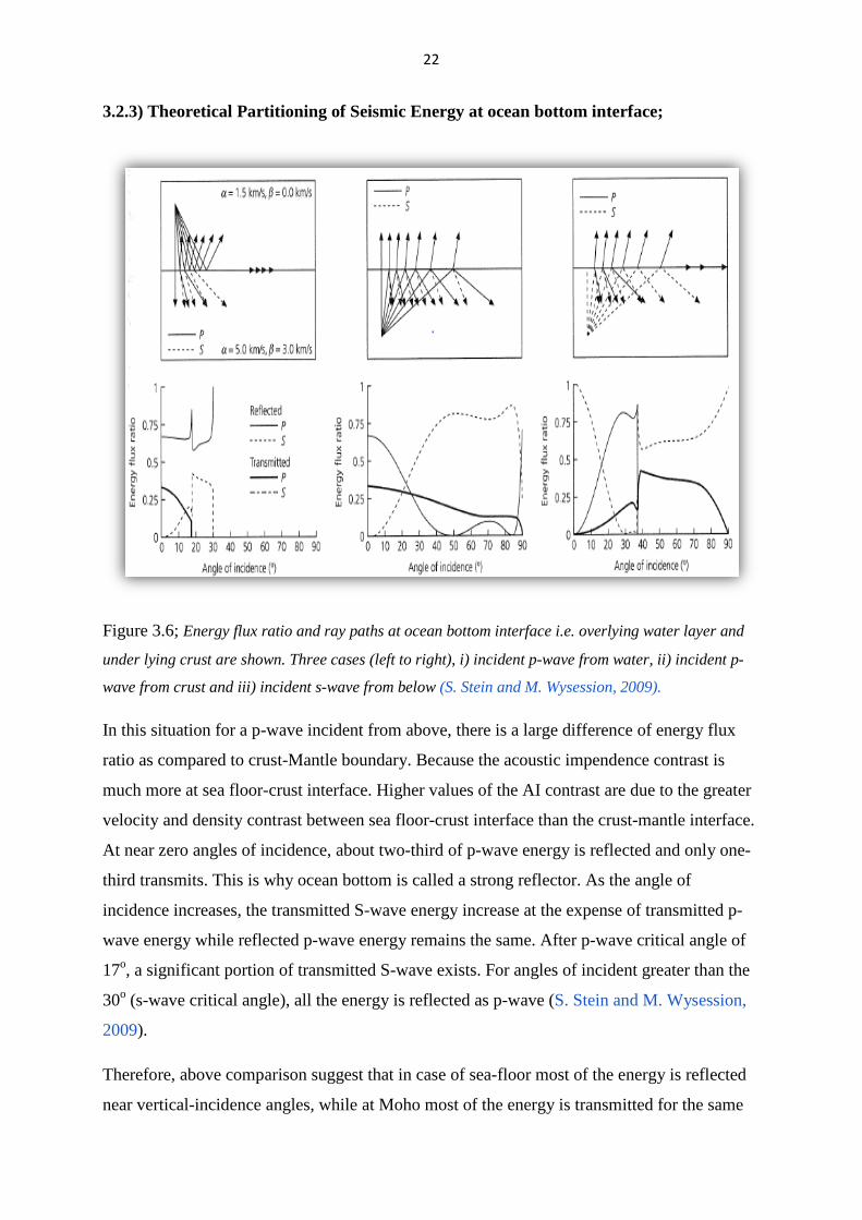
3.2.3) Theoretical Partitioning of Seismic Energy at ocean bottom interface;
Figure 3.6; Energy flux ratio and ray paths at ocean bottom interface i.e. overlying water layer and
under lying crust are shown. Three cases (left to right), i) incident p-wave from water, ii) incident p-
wave from crust and iii) incident s-wave from below (S. Stein and M. Wysession, 2009).
In this situation for a p-wave incident from above, there is a large difference of energy flux
ratio as compared to crust-Mantle boundary. Because the acoustic impendence contrast is
much more at sea floor-crust interface. Higher values of the AI contrast are due to the greater
velocity and density contrast between sea floor-crust interface than the crust-mantle interface.
At near zero angles of incidence, about two-third of p-wave energy is reflected and only one-
third transmits. This is why ocean bottom is called a strong reflector. As the angle of
incidence increases, the transmitted S-wave energy increase at the expense of transmitted p-
wave energy while reflected p-wave energy remains the same. After p-wave critical angle of
17o, a significant portion of transmitted S-wave exists. For angles of incident greater than the
30o (s-wave critical angle), all the energy is reflected as p-wave (S. Stein and M. Wysession,
2009).
Therefore, above comparison suggest that in case of sea-floor most of the energy is reflected
near vertical-incidence angles, while at Moho most of the energy is transmitted for the same
23
angle ranges. Similarly, in S-wave case, since α1 > β2 in Moho case, so there exists no critical
angle of S-wave. At the ocean-bottom interface good amount of p-wave energy is converted
to transmit S-wave until S-wave critical angle is reached (S. Stein and M. Wysession, 2009).
Similarly, the results for the two cases are also different for a p-wave incident from below. In
this case, most of the p-wave is reflected downward up to the angle of incidence of 20o. After
this angle, most of the reflected energy is in the form of S-wave reflection. However, in Moho
case negligible S-wave reflection takes place and most of the energy is transmitted as p-wave
until grazing angle, where reflected p-wave dominates (S. Stein and M. Wysession, 2009).
From above example it’s clear that a p-wave incident at ocean bottom interface from above
give rise to significant amount of S-wave energy and an S-wave incident at ocean bottom
interface from below results in substantial amount of transmitted p-wave energy. This fact can
be used to study the earth in terms of converted S-waves from incident p-waves at ocean
bottom interface. These waves travel down the earth as s-waves and can be recorded at the
surface as converted p-waves from s-waves at the ocean bottom interface (S. Stein and M.
Wysession, 2009).
The above situation could not be applied to our study area as the acoustic contrast at sea-floor
bottom is not so much higher in our case. In above case the p-wave velocity in the crust is 5
km/s while in our case its range is between 1.5-2 km/s. Still most of the s-wave arrivals at
OBS’s have been interpreted to be converted s-waves at ocean-bottom or very shallow
interfaces.
However, in our study area as the Profile-3-03 and Profile-4-03 span from land to sea,
therefore two different types of conversion interfaces are observed. For Ocean Bottom
Seismometers (OBS) the sea floor or upper shallower interfaces act like a dominant
conversion interfaces and majority of the p to s-wave conversions takes place at ocean-bottom
or very shallow interfaces. In case of Land-stations the dominant conversion interfaces are
represented by the various basement layers. In this case most of the p to s-wave conversions
takes place at different basement layers on their way up.
3.3) Poisson Ratio;
Poisson ratio is defined at the ratio of the transverse contracting strain to the longitudinal
extensional strain. Usually it is represented by a Greek Symbol sigma, σ.
24
Figure 3.7; Figure showing concept of Poisson ratio.
Mathematically,
𝜎 = 𝑒𝑦 𝑒𝑥� (3.6)
Where 𝑒𝑥 Rrepresents strain in x-direction and 𝑒𝑦 denotes strain along y-direction while 𝜎R
represents Poisson ratio.
The advantage of Poisson ratio is its direct linkage to the material properties which can be
measured in the field i.e. P-wave and S-wave velocities (Christensen, 1996).
Mathematically, in terms of p and s-wave velocities it can be written as; (Christensen, 1996)
𝜎 = 12
�1 − 1
�𝑉𝑃 𝑉𝑆� �2−1� (3.7)
Where Vp = P-wave velocity.
And Vs = S-wave velocity.
Since in fluids, Vs = 0, so Poisson ratio is 0.5. Average Poisson ratio for continental crust is
0.265 while for oceanic crust is 0.30 (Svetlov et al., 1988).
25
4) Forward Seismic Modeling Methodology;
4.1.1) Introduction;
Ray Tracing is used to model the complex geological structures both in 2D and 3D domain.
Its basic principle is to calculate the path of seismic energy during its propagation from source
to receiver and estimating the associated amplitudes and time of travel. It began with the
development of ray tracing algorithms, i.e. Cerveny et al. (1977), Spence et al. (1984) and
Luetgert (1992).
Because of its simplicity, applicability and easy to understand nature it is widely used for
solution of forward and inverse seismological problems. Its application also includes Seismic
Tomography and studying the relatively deep geological structures (Julian and Gubbins,
1977).
The travel time forward inversion algorithms developed by Zelt and Smith in 1992 are widely
used and are termed as ZS92. These are also the basis of RAYINVR software used for
modeling of s-wave in this thesis. It has following distinctions from its counterparts,
(modified from Colin A. Zelt, 1999).
• Addition of floating reflectors which don’t follow the general velocity field trend.
• Layer interfaces and velocity can be tied.
• Interfaces depths and velocity nodes can be distributed randomly.
• All types of arrivals can be modeled at the same time.
The inclusion of above features allows induction of any previous geological and geophysical
information into the velocity model. It also serves to model the sparsely acquired wide angle
OBS data to be modeled with better accuracy (Zelt and White 1995).
4.1.2) Identification of Arrivals/Signals;
In order to trace rays and develop a subsurface velocity model first step is the correct
identification of seismic signals from seismic stations, in this case ocean-bottom
seismometers (OBS). Accuracy and certainty of a model developed by interpretation of wide
angle OBS data is directly related to the identification of accurate arrivals. Therefore, the
most distinct arrivals, which are the 1st arrivals, are picked first. Then an initial model is
developed and is continuously upgraded as more and later arrivals are interpreted. Knowledge
of tectonic settings of the area could also be used to make logical predications of the onset of
26
arrivals. Since the wide angle OBS data is mostly acquired on existing ordinary reflection
profiles, so those can also be used to help identify the signals. In sparse and bad quality data,
care should be taken not to interpolate the observed events for a smoothed model, as this will
result in an inaccurate velocity model. (Colin A. Zelt, 1999).
Automatic picking scheme is seldom used for OBS data because of strong noise, phase
changes over larger offsets and weaker signals embedded in large amplitude coda. (Colin A.
Zelt, 1999).
Therefore, manual picking scheme was used for the picking of the s-wave signals in this
thesis. In this scheme few picks are picked using hand and the intervening signals are picked
by the interpolation between the two adjacent hand-picked signals.
27
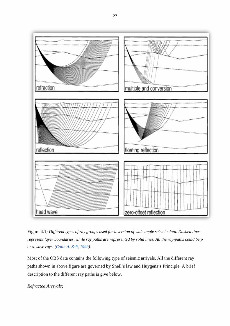
Figure 4.1; Different types of ray groups used for inversion of wide angle seismic data. Dashed lines
represent layer boundaries, while ray paths are represented by solid lines. All the ray-paths could be p
or s-wave rays. (Colin A. Zelt, 1999).
Most of the OBS data contains the following type of seismic arrivals. All the different ray
paths shown in above figure are governed by Snell’s law and Huygens’s Principle. A brief
description to the different ray paths is give below.
Refracted Arrivals;
28
When a ray enters from a lower velocity medium into a higher one, it is refracted away from
the normal while it bends towards the normal upon entering from higher to lower velocity
medium. In RAYINVR program, the layer in which refracted ray bottoms, should be chosen
with caution. It is because that most of the algorithms trace the refracted ray to the travel time
that satisfies the earliest arrival at any receiver before comparing this with the observed data.
So, due to this refracted phases represent a smooth variation in time with offset and don’t
exhibit obvious changes in the slope of the arrivals. It should be interpreted as a velocity
model with continuous variation with depth rather than a having sharp discontinuities (Colin
A. Zelt, 1999).
Multiples;
Any seismic signal/wave that has experienced more than one reflection is called multiple.
These can have long or short lag from the primaries and are regarded as noise. In wide angle
OBS data mostly only the 1st arrivals are picked so there is usually no need to process the
data for multiples removal.
Reflections;
When a seismic wave impinges on a lithological boundary having acoustic impedance
contrast, a portion of its energy is reflected back. As in most of the cases, most of the energy
is transmitted, so reflection amplitudes are very less and are difficult to observe in wide angle
OBS Data. However, in our data, significant amount of reflected waves can be interpreted,
originating from sediment-basement and basement-Mantle interface. Both of these interfaces
have relatively large acoustic contrasts resulting in detectable reflection strengths.
Floating Reflector;
A floating refection corresponds to an interface that is not necessarily associated with a
velocity boundary. It may arise of any localized rock inclusion having different velocity than
the general velocity trend resulting in acoustic contrast. In this thesis since signal quality is
already poor, so it was not expected to distinguish any such event. Thus, it was omitted from
modeling.
Head Wave;
29
These are generated when there is positive velocity contrast between upper and lower velocity
layers. For a wave that impinges on the higher velocity layer at critical angle, head waves are
generated.
Zero-offset Reflection,
It is produced when source and receiver are at the same location i.e. no source-receiver
separation.
4.1.3) Uncertainty of the Interpretation/Picks;
To avoid over or under-matching of observed and calculated travel times, uncertainty values
should be assigned to each pick. A suitable uncertainty value is dependent upon several
factors i.e. S/N ratio, amplitude/frequency of the arrivals and overall quality of the data.
Observed and calculated travel time picks are calculated by a mis-fit parameter, called chi-
squared denoted by “χ²” (Bevington, 1969). A value of χ²=1 corresponds that data has been
adjusted according to the specified uncertainties without over or under-fitting. Generally if
overall value of χ²<1 or χ²>1, it means that model is over or under-fit and it contains details
which are not present or vice versa (C. A. Zelt, 1994).
However, this condition is still acceptable if there are very less data points to obtain the
suitable chi-values statistically. But, only χ² values are not the sole criteria to judge the
accuracy of the model. Resolution of the model and ray-coverage density is also very much
important. Therefore, in case of poor quality data, the value of uncertainties can be increased
logically to make the χ² values near to 1 (C. A. Zelt, 1994).
4.1.4) Reciprocity of Travel times;
In order to get consistent interpretation, reciprocal source-receiver pairs must have the same
travel times for the same arrivals. Differences of travel times larger than the uncertainty
values must be removed before modeling (C. A. Zelt, 1994).
4.2) Modeling Strategy;
Crustal data interpretation is mostly carried out by forward-modeling using a trial and error
technique on 2D profile. The theoretical travel time responses of subsurface stratum are
compared with observed ones. This trial and error technique results in a velocity model which
best matches between theoretical and observed travel times. A number of ray tracing
30
algorithms has been developed from time to time based on ray theory (Cerveny et al., 1977)
i.e. McMechan and Mooney (1980), Cerveny and Psencik (1981), Cassell (1982) and Spence
et al. (1984), (C.A. Zelt, 1988).
Velocity parameterization is a distinguishing factor of any algorithm. For any algorithm, the
efficiency, accuracy and practicality is directly linked with its velocity parameters (C.A Zelt,
1988).
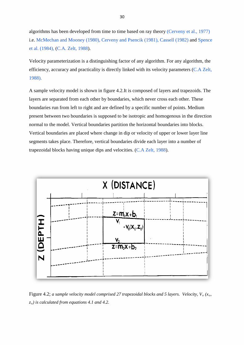
A sample velocity model is shown in figure 4.2.It is composed of layers and trapezoids. The
layers are separated from each other by boundaries, which never cross each other. These
boundaries run from left to right and are defined by a specific number of points. Medium
present between two boundaries is supposed to be isotropic and homogenous in the direction
normal to the model. Vertical boundaries partition the horizontal boundaries into blocks.
Vertical boundaries are placed where change in dip or velocity of upper or lower layer line
segments takes place. Therefore, vertical boundaries divide each layer into a number of
trapezoidal blocks having unique dips and velocities. (C.A Zelt, 1988).
Figure 4.2; a sample velocity model comprised 27 trapezoidal blocks and 5 layers. Velocity, Vo (xo,
zo) is calculated from equations 4.1 and 4.2.
31
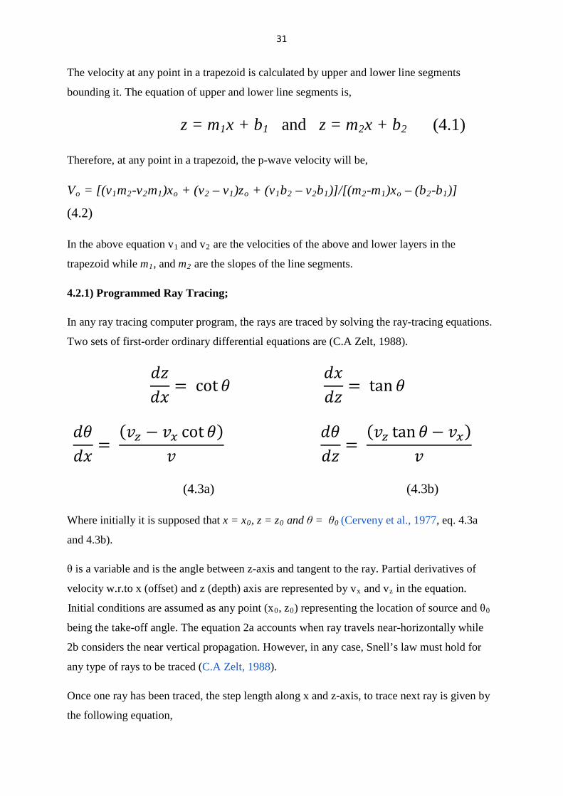
The velocity at any point in a trapezoid is calculated by upper and lower line segments
bounding it. The equation of upper and lower line segments is,
z = m1x + b1 and z = m2x + b2 (4.1)
Therefore, at any point in a trapezoid, the p-wave velocity will be,
Vo = [(v1m2-v2m1)xo + (v2 – v1)zo + (v1b2 – v2b1)]/[(m2-m1)xo – (b2-b1)]
(4.2)
In the above equation v1 and v2 are the velocities of the above and lower layers in the
trapezoid while m1, and m2 are the slopes of the line segments.
4.2.1) Programmed Ray Tracing;
In any ray tracing computer program, the rays are traced by solving the ray-tracing equations.
Two sets of first-order ordinary differential equations are (C.A Zelt, 1988).
𝑑𝑧𝑑𝑥 = cot 𝜃
𝑑𝑥𝑑𝑧 = tan𝜃
𝑑𝜃𝑑𝑥
= (𝑣𝑧 − 𝑣𝑥 cot 𝜃)
𝑣 𝑑𝜃𝑑𝑧 =
(𝑣𝑧 tan𝜃 − 𝑣𝑥)𝑣
(4.3a) (4.3b)
Where initially it is supposed that x = x0, z = z0 and θ = θ0 (Cerveny et al., 1977, eq. 4.3a
and 4.3b).
θ is a variable and is the angle between z-axis and tangent to the ray. Partial derivatives of
velocity w.r.to x (offset) and z (depth) axis are represented by vx and vz in the equation.
Initial conditions are assumed as any point (x0, z0) representing the location of source and θ0
being the take-off angle. The equation 2a accounts when ray travels near-horizontally while
2b considers the near vertical propagation. However, in any case, Snell’s law must hold for
any type of rays to be traced (C.A Zelt, 1988).
Once one ray has been traced, the step length along x and z-axis, to trace next ray is given by
the following equation,
32
∆ = 𝛼𝑣|𝑣𝑥|+|𝑣𝑧|
(4.4)
Above equation reveals that in case of strong lateral (vx)or vertical (vz)velocity gradients, the
ray step length will be small and vice versa. It is because of the fact that in case of strong
velocity gradients, large ray bending will occur. Therefore, in order to trace rays accurately,
the step length must be smaller. Alpha α, is constant and supplied by the user and it serves as
a guarantee to trace the rays with accuracy and efficiency (C.A Zelt, 1988).
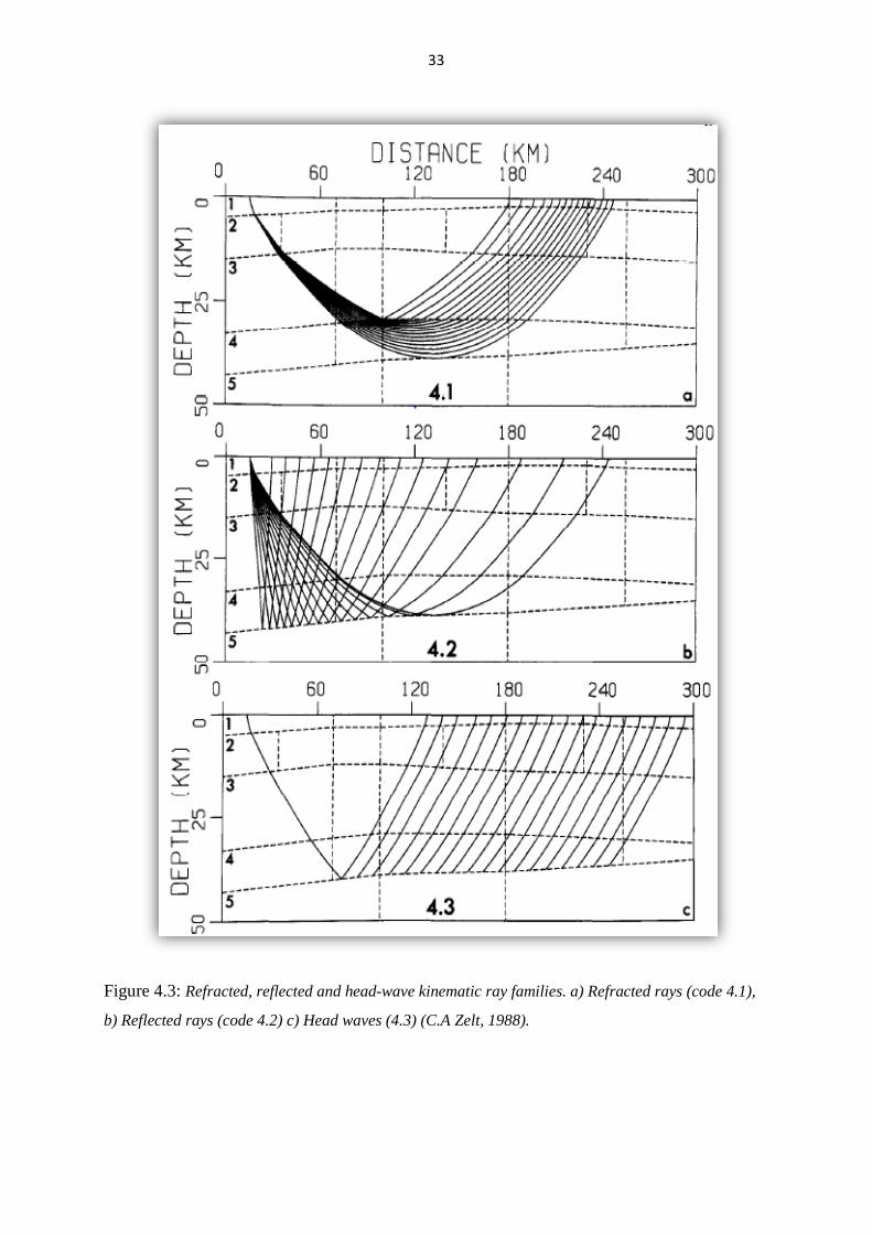
In the ray-tracing program three main kinematic ray families are searched based upon their
ray- takeoff angles (calculated from the horizontal), in any model layer as shown in figure 4.3.
It includes (C.A Zelt, 1988).
Refracted Rays; which refract in the layer. For this class, first the search mode determines
the take-off angle of the uppermost and lowermost refracted rays in the layer. Once the upper
and lower limit of the take-off angles has been determined, it traces the intermediate family
rays according to the maximum number of allowed rays within these limits.
Reflected Rays; This family of rays reflect from the bottom of the layer. In reflected family
case, first the smallest take-off angle for the reflected is determined in search mode. Once it
has been established, then other family rays are traced from this smallest angle up to
maximum angle (mostly 900) i.e. vertical.
Head Waves; Such kind of waves propagate along the top of the layer. For such kind of ray
family, the search mode looks for those rays which strike the upper boundary of the layer at
critical angle. Thus all those rays which emerge at this angle are traced to give a family of
head waves.
33
Figure 4.3: Refracted, reflected and head-wave kinematic ray families. a) Refracted rays (code 4.1),
b) Reflected rays (code 4.2) c) Head waves (4.3) (C.A Zelt, 1988).
34
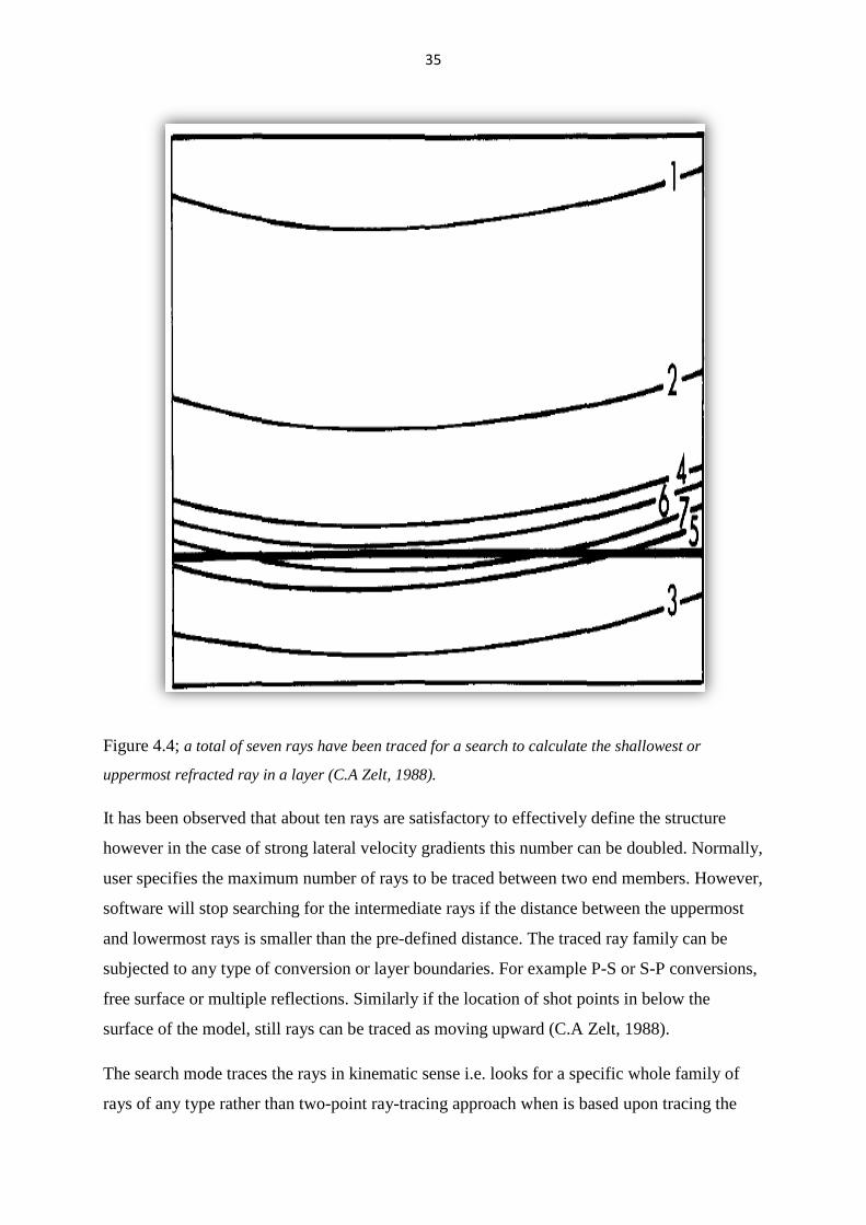
4.2.2) Ray Search Mode;
Search mode operates similar for all the three ray types. Let us take the example of
determining the take-off angle of an uppermost refracted ray in any layer. For a medium with
no lateral variation of the velocity i.e. laterally homogenous, the take-off angle Φ0 from the
horizontal can be written as, (C.A Zelt, 1988).
Φ0 = 90° − sin−1 �v0 v� � (4.5)
In above equation ‘v0’represents velocity function at the source and ‘v’ denotes the velocity at
the top of the specified layer. After tracing the first ray, a second ray is traced using a take-off
angle of (Φ0 + ∂Φ) if the first ray did not enter the layer or by (Φ0 - ∂Φ), if first ray entered
the layer. Where ∂Φ represents a specified portion of the angle difference between uppermost
and lowermost take-off angles calculated in the search mode i.e. |Φ⃰0 - Φ0|. In previous case if
the first or second rays did not bisected the layer boundary a new set of rays will be traced
using angle (Φ0 + 1/2∂Φ) and (Φ0 – 1/2∂Φ). This practice will be continued until the traced
rays bisect the layer boundary as shown in the figure 4.4 (C.A Zelt, 1988).
35
Figure 4.4; a total of seven rays have been traced for a search to calculate the shallowest or
uppermost refracted ray in a layer (C.A Zelt, 1988).
It has been observed that about ten rays are satisfactory to effectively define the structure
however in the case of strong lateral velocity gradients this number can be doubled. Normally,
user specifies the maximum number of rays to be traced between two end members. However,
software will stop searching for the intermediate rays if the distance between the uppermost
and lowermost rays is smaller than the pre-defined distance. The traced ray family can be
subjected to any type of conversion or layer boundaries. For example P-S or S-P conversions,
free surface or multiple reflections. Similarly if the location of shot points in below the
surface of the model, still rays can be traced as moving upward (C.A Zelt, 1988).
The search mode traces the rays in kinematic sense i.e. looks for a specific whole family of
rays of any type rather than two-point ray-tracing approach when is based upon tracing the

36
rays up to a specific receiver (cf. Cassell, 1982). Kinematic ray tracing has the advantage that
a specific portion of the model can be studied using a specific family of rays (C.A Zelt, 1988).
37
5) Processing of wide-angle seismic data;
It is almost impossible to extract any geological information from the raw data acquired in the
field. Therefore, it must be processed. Basically, processing consists of a series of computer
routines which are applied on the raw data. It increases the signal to noise ratio and results in
interpretability of the data.
Processing of OBS data was carried out in Seismic Unix. In our case the following steps were
used.
Velocity reduction
Band-pass filtering
Automatic gain Control (AGC)
Spiking Deconvolution
Rotation of the horizontal components of OBS and Land Data.
Above processing steps are explained in detail below.
5.1) Velocity Reduction;
It is done by changing the time axis to (time – offset/V.red). V.red denotes the reduction
velocity. Reduction velocity is chosen on the basis of objective of the study and it aids in the
interpretation of the arrivals. In crustal scale refraction studies, the data is often reduced by
8km/s. It is because of the fact that P-wave velocity in the upper mantle is of this magnitude.
However, in our case, as the purpose was to enhance s-wave arrivals, a reduction velocity of
4.62km/s was applied because it represents s-wave velocity in upper mantle. In this way s-
wave arrivals from upper mantle or Moho appear as near horizontal events, and are easily
identifiable. Similarly those arrivals which have lower apparent velocities than the V. red
appear as having positive slopes and vice versa as shown in the figure 5.2 below. Positive
slope means that for any family of s-wave arrivals, as the offset increases from the OBS
location, it arrives at later times at farther traces. Whereas, the term negative slope suggests
that farther offset arrivals come at lesser times for any family of ray paths.
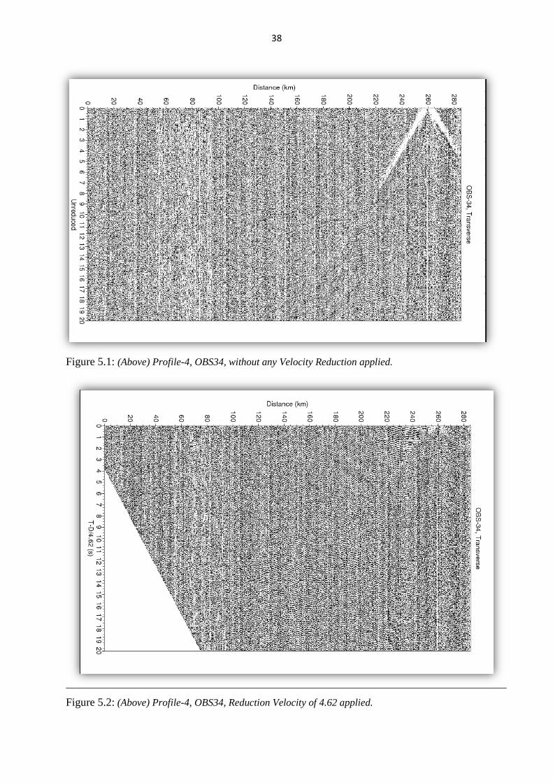
38
Figure 5.1: (Above) Profile-4, OBS34, without any Velocity Reduction applied.
Figure 5.2: (Above) Profile-4, OBS34, Reduction Velocity of 4.62 applied.

39
5.2) Band-pass filtering;
The recorded seismic data contains both signal and noise. Signal is that portion of data which
carries subsurface geological information while noise consists of all the remaining portion.
Noise can be further subdivided into two types based upon its appearance in the seismogram,
i.e. random and coherent.
Random noise does not show any specific pattern and is mostly connected with factors not
related to the survey for e.g. wind, vehicles, rain or any vibration caused by marine traffic.
While coherent noise follows a distant pattern and shows continuity from trace to trace. It
may distort the seismic signal. Its definition is based upon the nature of investigation being
carried out. For example in case of wide-angle OBS survey, refracted arrivals represent
signals while in reflection surveys, they are classified as coherent noise. Other examples of
coherent noise include, cable noise, multiples, diffractions, direct waves and out of plane
reflections.
There are various ways to remove seismic noises. Mostly frequency filtering of the seismic
data is used to get rid of noises. It is particularly helpful when signal and noise have different
frequency spectra.
In our case a band pass filter 4-6-14-16 was used to suppress the noises. It allows passing only
those frequencies which are above 4 Hz and lower than 16 Hz.
Figure 5.5; Bandpass filter, F(Hz) represents frequency spectrum of the output. F1=4, F2=6, F3=14
and F4=16 (Source= SeisView)
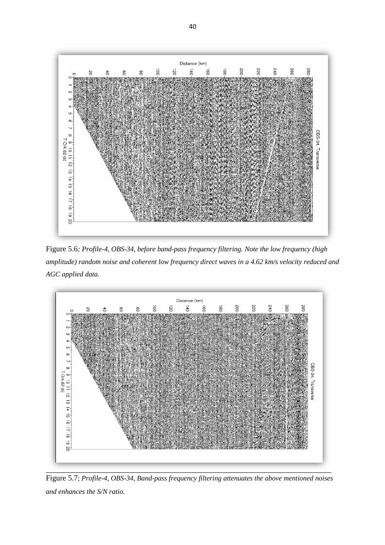
40
Figure 5.6; Profile-4, OBS-34, before band-pass frequency filtering. Note the low frequency (high
amplitude) random noise and coherent low frequency direct waves in a 4.62 km/s velocity reduced and
AGC applied data.
Figure 5.7; Profile-4, OBS-34, Band-pass frequency filtering attenuates the above mentioned noises
and enhances the S/N ratio.
41
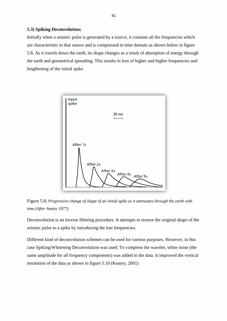
5.3) Spiking Deconvolution;
Initially when a seismic pulse is generated by a source, it contains all the frequencies which
are characteristic to that source and is compressed in time domain as shown below in figure
5.8. As it travels down the earth, its shape changes as a result of absorption of energy through
the earth and geometrical spreading. This results in loss of higher and higher frequencies and
lengthening of the initial spike.
Figure 5.8; Progressive change of shape of an initial spike as it attenuates through the earth with
time (After Anstey 1977).
Deconvolution is an inverse filtering procedure. It attempts to restore the original shape of the
seismic pulse to a spike by introducing the lost frequencies.
Different kind of deconvolution schemes can be used for various purposes. However, in this
case Spiking/Whitening Deconvolution was used. To compress the wavelet, white noise (the
same amplitude for all frequency components) was added to the data. It improved the vertical
resolution of the data as shown in figure 5.10 (Kearey, 2001)
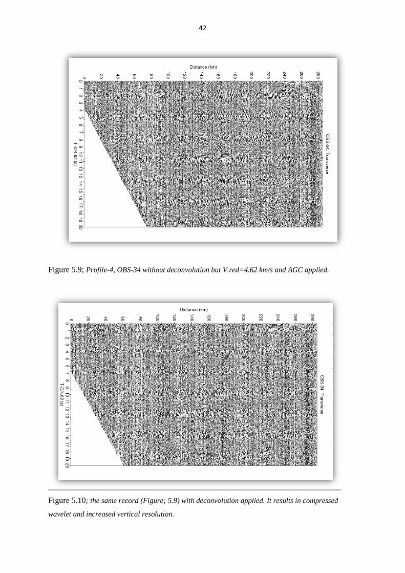
42
Figure 5.9; Profile-4, OBS-34 without deconvolution but V.red=4.62 km/s and AGC applied.
Figure 5.10; the same record (Figure; 5.9) with deconvolution applied. It results in compressed
wavelet and increased vertical resolution.
43
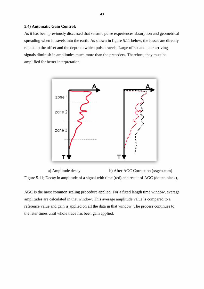
5.4) Automatic Gain Control;
As it has been previously discussed that seismic pulse experiences absorption and geometrical
spreading when it travels into the earth. As shown in figure 5.11 below, the losses are directly
related to the offset and the depth to which pulse travels. Large offset and later arriving
signals diminish in amplitudes much more than the preceders. Therefore, they must be
amplified for better interpretation.
a) Amplitude decay b) After AGC Correction (xsgeo.com)
Figure 5.11; Decay in amplitude of a signal with time (red) and result of AGC (dotted black),
AGC is the most common scaling procedure applied. For a fixed length time window, average
amplitudes are calculated in that window. This average amplitude value is compared to a
reference value and gain is applied on all the data in that window. The process continues to
the later times until whole trace has been gain applied.
44
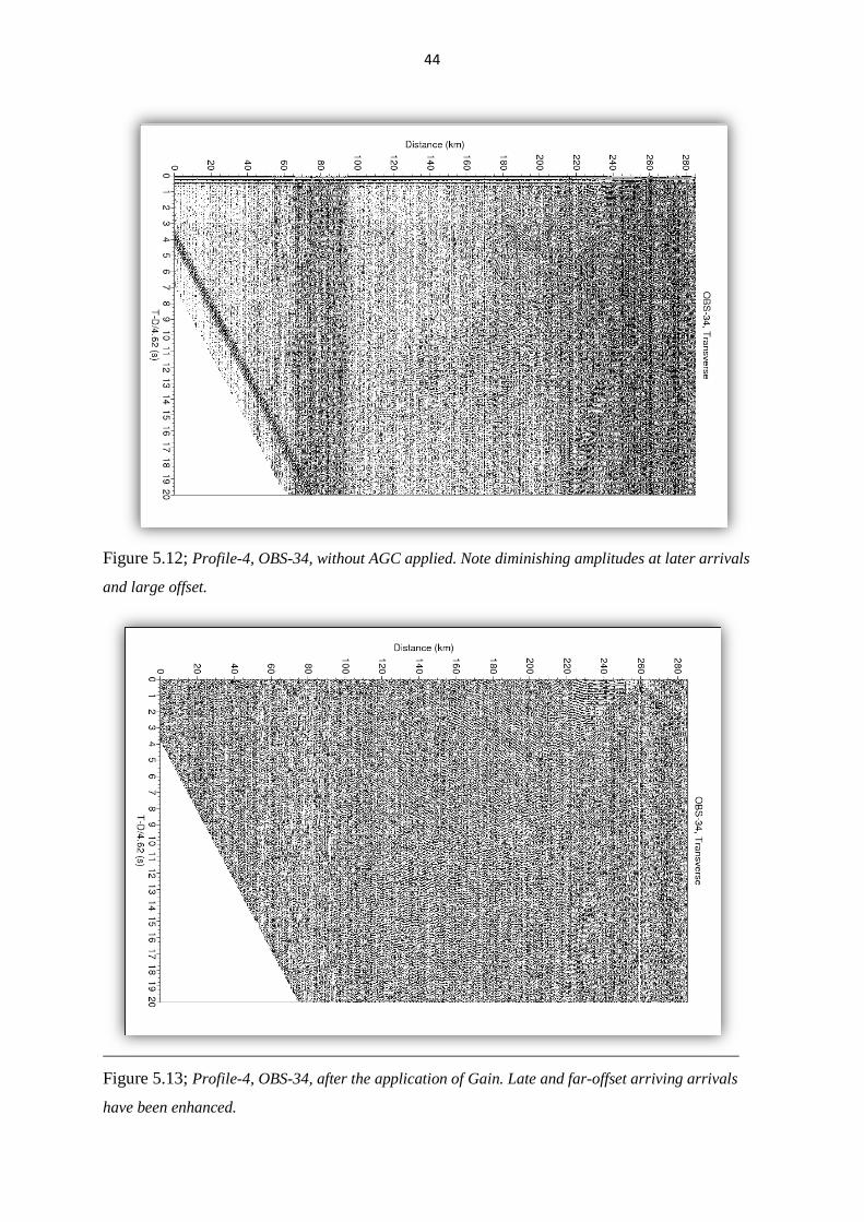
Figure 5.12; Profile-4, OBS-34, without AGC applied. Note diminishing amplitudes at later arrivals
and large offset.
Figure 5.13; Profile-4, OBS-34, after the application of Gain. Late and far-offset arriving arrivals
have been enhanced.
45
5.5) Rotation of the Data;
Since 3-C Ocean bottom seismometers sink into ocean as free falling objects, their horizontal
components are not oriented into cross-line and in-line directions relative to the source. Their
alignment is completely arbitrary. We need to realign them relative to source-centered
common orientation (Gaiser, 1998).
Attempt was made to realign all the 3-C OBS’s horizontal components parallel and
perpendicular to the source-receiver plane. Thus in this way the radial component points
towards the source, and will recored particle motion parallel to the source-receiver plane.
It has been observed that seismic signal which consists of reflections, refraction and head
waves have source-receiver direction as their main polarization plane. This means that using
above rotation scheme; signal should get stronger on radial component and minimum energy
should be present on transverse component (Gaiser, 1998).
In order to estimate the angles to rotation for horizontal components information of direct
wave travel time information was used. This wave travels direct from shot point to the OBS in
the water. Due to poor data quality it is not possible to pick direct wave phases on all the
stations. Therefore, another technique was used for such OBS-stations . OBS stations data
was rotated for 0o to 90o with a successive angle increment of 20o and was compared for every
angle increment. Those angles which gave improved quality relative to un-rotated ones were
selected for interpretation. After the rotation scheme first break arrivals showed improved
continuity on rotated OBS stations as shown in figure 5.15.
For majority of the seismometers, this scheme worked and resulted in relatively better data
quality. In case of land-stations since all of them had the fixed and same azimuthal
orientation, therefore, they were angle rotated by determining the azimuth of the profile lines
relative to north.
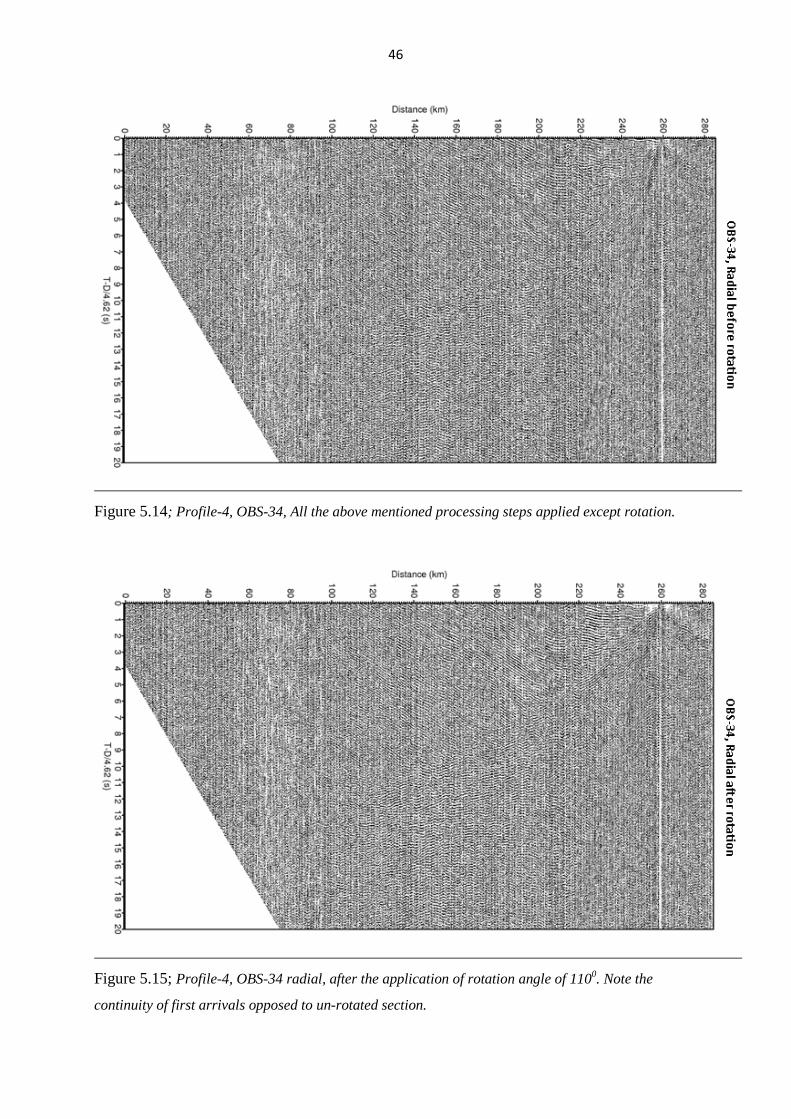
As shown in figure 5.15 below, a significant improvement in S/N ratio can be observed in the
OBS-34, radial- Component after the application of rotation angle of 110O. Although not
shown here, signal quality on OBS- 34, Transverse-Component decreases significantly
because of concentration of energy in the radial direction.
46
Figure 5.14; Profile-4, OBS-34, All the above mentioned processing steps applied except rotation.
Figure 5.15; Profile-4, OBS-34 radial, after the application of rotation angle of 1100. Note the
continuity of first arrivals opposed to un-rotated section.
47
6) Interpretation and Modeling of data;
After the processing step, converted shear wave phases were identified and modeled on radial
components of OBS’s of Profile-3-03 and 4-03.
The already generated p-wave models (Breivik et al, 2011) interpreted from vertical
component of seismometers were used as a base model for the interpretation and modeling of
converted s-waves identified on radial components. Free boundary reflectors interpreted by p-
wave data were not included in the modeling scheme as it is not expected to identify weak and
localized converted s-waves, originating from them. It was supposed that same p-wave
interface represent an s-wave interface.
The same software ‘RAYINVR’ was used for the s-wave modeling. It requires three
parameters for ray-tracing, i.e. conversion boundary, nature of conversion and Poisson ratio.
Nature of conversion means whether ray refract, reflect or propagate as head wave.
Although more than two p to s-conversions can be modeled however, energy loss for multiple
conversions is great so it is not expected to get strong signal in that case. Therefore, whole of
the modeling was limited to only one conversion i.e. from P to S.
As explained in the previous chapter, Poisson ratio specifies the relation between p and s-
wave velocities. Once we have provided the correct conversion interfaces and nature of
conversion, a suitable value for Poisson ratio should be provided iteratively so that observed
and calculated travel times fit each other.
All the OBS arrivals are assigned an uncertainty value for the actual arrival time of any signal
and the one interpreted by the interpreter. This value is based upon the confidence in picking
the arrivals. Normally, OBS arrivals closer to the OBS location are more certain and are given
low uncertainty values. The ease of picking decreases at farther offsets and so does the
uncertainty values. In our case since the data quality was already poor therefore uncertainty
values in the range of 150 to 250ms were assigned to different arrivals depending upon the
confidence in picking the arrivals.
As shown in figure below, various s-wave phases were identified. The whole of the horizontal
components has been applied 4.62 km/s reduction velocity to enhance the s-wave arrivals.

48
6.1) Classification of Arrivals;
Following class of s-wave arrivals were identified,
PPS Arrivals; these kind of arrivals are recorded quite early in time. It is because that seismic
energy travels most of its path at high velocity i.e. as p-waves. However, when it reaches to
shallower interfaces on its way back to receiver; it is converted from p to s-wave and recorded
as an s-wave. As it travels most of its path with higher apparent velocities than the reduction
velocity of 4.62 km/s, it has negative slope as shown in figure 6.1 below.
PSS Arrivals; It comprises converted s-wave energy when p-waves are converted to s-waves
on their way down in the model. Therefore, it arrives at later times and has a positive slope.
SS-wave (Sg) arrivals are a special kind of PSS arrivals. These are identified as s-wave
energy which is generated by the conversion of p to s-wave at the ocean-bottom interface on
their way down. After this it travels whole of its propagation path as an s-wave. As s-waves
travel at lower apparent velocities than p-waves, such arrivals are one of the last to be
recorded.
Figure 6.1; Profile-OBS39, radial, different arrivals highlighted. (Explained in text)
49
SmS Arrivals; Such kind of arrivals represent reflected s-waves at Moho. After converting
from p to s-waves at ocean-bottom interface, these travel nearly whole of their journey as s-
waves.
PSP Arrivals; Such kind of waves start their journey as a p-wave, however, these are
converted two times. One from p to s-wave then 2nd time from s to p-wave again. These
arrivals are recorded primarily on vertical-components of 3-C seismometers. However, in our
case these arrivals were not modeled because due to two conversions, very less energy is
recorded on seismometers and were not possible to identify any of it within acceptable
uncertainty ranges.
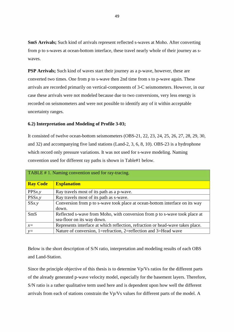
6.2) Interpretation and Modeling of Profile 3-03;
It consisted of twelve ocean-bottom seismometers (OBS-21, 22, 23, 24, 25, 26, 27, 28, 29, 30,
and 32) and accompanying five land stations (Land-2, 3, 6, 8, 10). OBS-23 is a hydrophone
which record only pressure variations. It was not used for s-wave modeling. Naming
convention used for different ray paths is shown in Table#1 below.
TABLE # 1. Naming convention used for ray-tracing.
Ray Code Explanation
PPSx.y Ray travels most of its path as a p-wave. PSSx.y Ray travels most of its path as s-wave. SSx.y Conversion from p to s-wave took place at ocean-bottom interface on its way
down. SmS Reflected s-wave from Moho, with conversion from p to s-wave took place at
sea-floor on its way down. x= Represents interface at which reflection, refraction or head-wave takes place. y= Nature of conversion, 1=refraction, 2=reflection and 3=Head wave
Below is the short description of S/N ratio, interpretation and modeling results of each OBS
and Land-Station.
Since the principle objective of this thesis is to determine Vp/Vs ratios for the different parts
of the already generated p-wave velocity model, especially for the basement layers. Therefore,
S/N ratio is a rather qualitative term used here and is dependent upon how well the different
arrivals from each of stations constrain the Vp/Vs values for different parts of the model. A
50
poor s-wave data quality could be a result of different factors. For e.g. shear waves lose their
amplitudes in the crust faster than the p-waves. Masking of shear wave arrivals by scattered p-
wave energy and multiple p to s-wave conversions also reduce S/N quality of the shear wave
data.
OBS-21; It has a relatively poor data quality with only two identifiable first arrivals
interpreted to be s-waves converted at ocean-bottom interface on the way down. Similarly
both the arrivals have been modeled to be refracted ones and refraction took place at
sediment-basement boundary. Although these travel as s-waves they are recorded relatively
early because of their shallow paths.
OBS-22; it also has poor data quality. Only three s-wave arrivals can be seen. The upper two
arrivals are refractions from sediment-basement boundary, while the third represent a high
velocity reflection from 3rd basement interface. Their positive dips at 4.62 km/sec reduction
velocity conform that these are s-wave-arrivals.
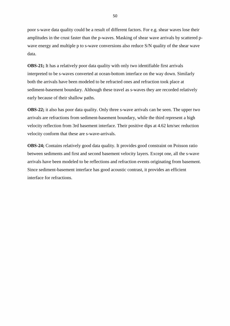
OBS-24; Contains relatively good data quality. It provides good constraint on Poisson ratio
between sediments and first and second basement velocity layers. Except one, all the s-wave
arrivals have been modeled to be reflections and refraction events originating from basement.
Since sediment-basement interface has good acoustic contrast, it provides an efficient
interface for refractions.
51
Figure 6.2; Profile-3, OBS-24. Upper window; traced rays. Lower Window; Bold color lines
represent interpreted arrivals while narrow black lines show the calculated arrivals by ray-tracing.
OBS-25; Data quality is poor, but provides relatively reliable constraint on 3rd basement
layer. Four converted s-wave arrivals can be seen. Two arrivals on the right side are head
wave from the top-basement while on left are high apparent velocity reflections from 2nd and
3rd basement layer. Sub-horizontal appearance of late arriving signal suggest that they
propagated as s-waves deep into crust.
OBS-26; it has quite poor data quality and only two refractions can be identified originating
from lower sediment layers. However, it could constrain Poisson ratio for sediments in 120-
150 km interval.
OBS-27; All the Arrivals have been interpreted to be originating from top-basement or
sedimentary layers above. It doesn’t provide any constrain on basement layers, however, it
does limit Poisson ratios for overlying sedimentary strata.
52
OBS-28; it also exhibit quite poor data quality and arrivals can be interpreted with limited
continuity. Ray coverage is limited only to the sedimentary strata. Noise level is quite high in
this data as compared to other ones probably due to some instrumental problem. Only two
PPS and less continuous SS arrivals can be modeled.
OBS-29; Data quality is very poor on this record. Only few arrivals can be interpreted. It may
provide constrain on Poisson ratio for sediments between 65-80 km. Although right hand side
arrivals don’t travel into deep crust, still they arrive late, which is because of most of their
travel through sediments at low angles.
OBS-30; Due to quite bad quality data, only two arrivals can be interpreted. Both the arrivals
are reflections, one from top of the basement and other from the Moho. Right hand side
arrival reflects from top of Moho and they appear as sub-horizontal in the seismic record. This
could also provide a good estimated of Vp/Vs ratio in the whole of the crust around 80-110
km offset.
OBS-31; it contains extremely poor data, and only one reflection event arriving from top of
Moho could be traced.
OBS-32; only one small reflection from top of basement can be traced. It could provide
constraints on Poisson ratio for upper sedimentary strata between 30-50 km.
Land station-2; although the data quality is poor on it, however, it still can constrain first and
second basement layers. Therefore, it provides good constraints on Poisson ratio for these
layers. All the three arrivals are p to s-converted at above mentioned layer boundaries. Near-
horizontal appearance of late arriving PPS suggest they travelled as p-wave for most of their
journey.
Land station-3; since Land-2 and Land-3 are located very close to each other, it exhibits
nearly the same arrivals as on Land-2 in terms of converting interfaces.
53
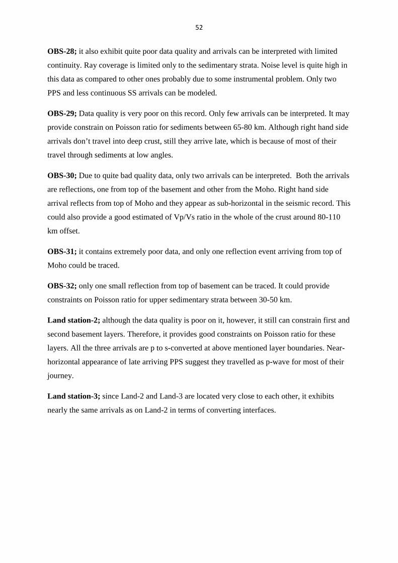
Figure 6.3; Profile-3, L. Station-3. Upper window; traced rays. Lower Window; Bold color lines
represent interpreted arrivals while narrow black lines show the calculated arrivals by ray-tracing.
Land-6 and 8; due to their closeness, the same kind of arrivals can be seen on them. Both
have only two refracted p to s-arrivals each, where conversion takes place at first and second
basement layers. Land stations provide quite good constrains on Poisson ratios for upper three
crustal layers between 200-280 kms.
Land-10; this station contains only one near offset head wave trapped in first basement layer.
6.3) Interpretation and Modeling of Profile 4-03;
This profile consists of eleven 3-C OBS (OBS-33, 34, 35, 37, 38, 39, 40, 42, 45 and 46) and
six 3-C Land Stations ( L-1, 2, 4, 5, 7 and 9). OBS-37 contained very poor data quality so was
not used for modeling of shear waves, and OBS-40 and L-4 contained very small amount of
54
data and it was not possible to perform any meaningful interpretation using them, so they
were skipped as well. The same naming convention given in Table#1 is used.
Below is the S/N ratio, interpretational and modeling summary of each of the stations.
OBS-33; Although, only three converted s-wave arrivals can be picked on it, still it
successfully constrain the first, second and fourth basement layer. All the three phases convert
on the ocean-bottom interface on their way down. Calculated reflection event from top of
Moho is in good agreement with the interpreted ones.
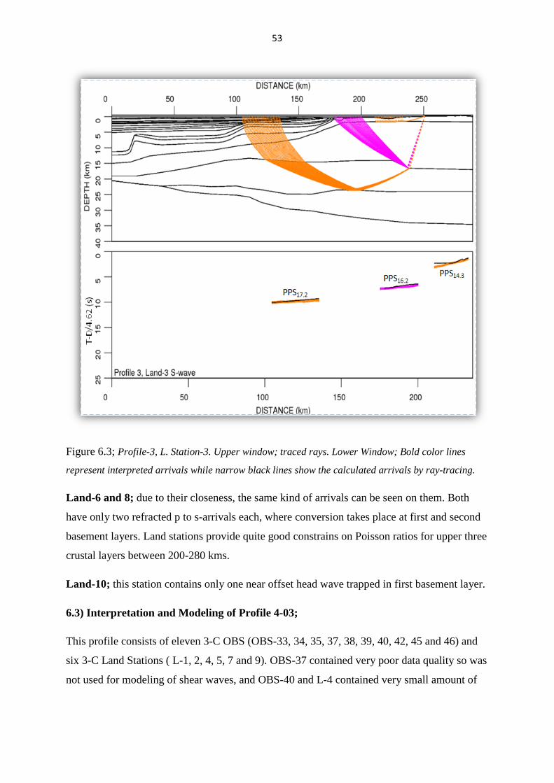
OBS-34; it exhibits almost the same behavior as the OBS-33. All the three interpreted arrivals
are p to s-converted at ocean-bottom interface on their way down.
Figure 6.4; Profile-4, OBS-34. Upper window; traced rays. Lower Window; Bold color lines
represent interpreted arrivals while narrow black lines show the calculated arrivals by ray-tracing.
OBS-35; the arrivals can be interpreted as converted s-waves and conversion took place on
the ocean-bottom interface on their way down. On the left side, converted s-wave has been
modeled to be reflecting from Moho while right side represent reflections from first and
second basement layers, respectively.
55
OBS-39; two PPS refractions can be identified on it. Their negative slopes and early arrivals
indicate that they travelled most of their journey as p-waves. However, two PSS arrivals can
also be identified reflecting from Moho.
OBS42; although it contains poor data quality; however it can serve as a guide for aggregated
Poisson ratio for all the basement layers. Because, it contains two refracted PSS arrivals from
top of mantle and one refracted PSS arrivals from sediment-basement interface.
OBS45; in spite of bad data quality, four PSS arrivals can be interpreted. Again these arrivals
constrain Poisson ratio for whole basement and partially its layers as well. All of these have
been modeled to be reflections from different basement layers.
OBS46; it is the last OBS sea-ward. It contains poor data quality with no arrivals at large
offset and later times. Only one head wave constraining upper sedimentary cover and two
reflections from first and second basement layers can be modeled.
Land-1; it has quite poor quality data and only one short-offset arrival can be identified and
has been modeled as PSS wave reflecting from second basement velocity layer. Data is quite
noisy so it is not possible to model long offset arrivals with confidence.
Land-2; this station is the further continuation of land stations. Three reflections can be
interpreted with confidence. All the three arrivals are PPS reflections. Two of them are
reflecting from Moho and one reflects from 3rd basement layer. However, these rays convert
from P to S at 1st, 3rd and fourth basement layer on their way up and provide a good relative
constrain on Poisson ratio for basement layers in 330-356 km.
Land-5; signal quality is quite poor and only two reflected PPS arrivals can be interpreted.
One is reflected as 3rd basement layer while the other one is from Moho. As p to s conversion
is taking place at 1st and 3rd basement layer, so an approximate estimate of Poisson ratios for
basement layers can be made for this offset range.
Land-7; L-5 and L-7 contain almost the same kind of events with same resolution. Due to
their closeness, traced rays follow approximately same path and are recorded at the same
approximate time. Similar case is with the S/N ratio, which is also bad.
Land-9; it shows up with slightly better data than the L-7 with one additional reflected
converted PSS wave, where conversion took place at Moho. So, it provides a good
approximation of Vp/Vs ratios for basement layers.
56
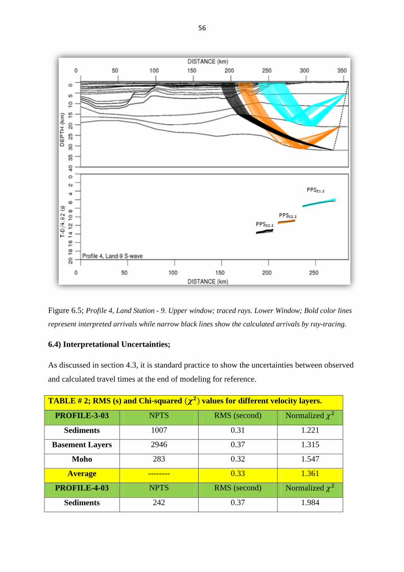
Figure 6.5; Profile 4, Land Station - 9. Upper window; traced rays. Lower Window; Bold color lines
represent interpreted arrivals while narrow black lines show the calculated arrivals by ray-tracing.
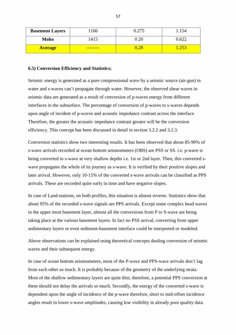
6.4) Interpretational Uncertainties;
As discussed in section 4.3, it is standard practice to show the uncertainties between observed
and calculated travel times at the end of modeling for reference.
TABLE # 2; RMS (s) and Chi-squared (𝝌𝟐)P
values for different velocity layers.
PROFILE-3-03 NPTS RMS (second) Normalized 𝜒2
Sediments 1007 0.31 1.221
Basement Layers 2946 0.37 1.315
Moho 283 0.32 1.547
Average -------- 0.33 1.361
PROFILE-4-03 NPTS RMS (second) Normalized 𝜒2
Sediments 242 0.37 1.984
57
Basement Layers 1166 0.275 1.154
Moho 1415 0.20 0.622
Average -------- 0,28 1.253
6.5) Conversion Efficiency and Statistics;
Seismic energy is generated as a pure compressional wave by a seismic source (air-gun) in
water and s-waves can’t propagate through water. However, the observed shear waves in
seismic data are generated as a result of conversion of p-waves energy from different
interfaces in the subsurface. The percentage of conversion of p-waves to s-waves depends
upon angle of incident of p-waves and acoustic impedance contrast across the interface.
Therefore, the greater the acoustic impedance contrast greater will be the conversion
efficiency. This concept has been discussed in detail in section 3.2.2 and 3.2.3.
Conversion statistics show two interesting results. It has been observed that about 85-90% of
s-wave arrivals recorded at ocean bottom seismometers (OBS) are PSS or SS. i.e. p-wave is
being converted to s-wave at very shallow depths i.e. 1st or 2nd layer. Then, this converted s-
wave propagates the whole of its journey as s-wave. It is verified by their positive slopes and
later arrival. However, only 10-15% of the converted s-wave arrivals can be classified as PPS
arrivals. These are recorded quite early in time and have negative slopes.
In case of Land-stations, on both profiles, this situation is almost reverse. Statistics show that
about 95% of the recorded s-wave signals are PPS arrivals. Except some complex head waves
in the upper most basement layer, almost all the conversions from P to S-wave are being
taking place at the various basement layers. In fact no PSS arrival, converting from upper
sedimentary layers or even sediment-basement interface could be interpreted or modeled.
Above observations can be explained using theoretical concepts dealing conversion of seismic
waves and their subsequent energy.
In case of ocean bottom seismometers, most of the P-wave and PPS-wave arrivals don’t lag
from each other so much. It is probably because of the geometry of the underlying strata.
Most of the shallow sedimentary layers are quite thin; therefore, a potential PPS conversion at
them should not delay the arrivals so much. Secondly, the energy of the converted s-wave is
dependent upon the angle of incidence of the p-wave therefore, short to mid-offset incidence
angles result in lower s-wave amplitudes, causing low visibility in already poor quality data.
58
Abundance of PPS arrivals on land stations could also be explained. As land stations lie
further SE from the last shot point, so already weaker PSS arrivals from far-offset shot points
loose more amplitude upon reaching them. While most of the PSS energy generated by near-
offset shot points between OBS-33 and 36, a very narrow part of the wave-front gets
converted into head wave and it is trapped as head wave inside the 1st shallow basement
layer. Thus preventing any PSS energy to travel down. However, situation for PPS energy is
different here, although, it still gets trapped inside 1st basement layer for shorter offsets.
However, for mid to large offsets, it travels most of its path in high velocity basement layers.
Therefore, it doesn’t lose energy quickly. When it is incident on basement layers from below,
high acoustic contrast serves as a perfect conversion interface. Similarly, in spite of travelling
in large vertical distance in basement layers, this energy is still detectable because of non-
dispersive nature of high-velocity basement layers.
This assumption could also be supported by the fact that PPS arrivals on OBS’s have negative
slope in 4.62 km/sec reduced seismic section, while PPS arrivals on Land-stations have
positive slope and are near-horizontal. Reason is that as PPS energy travel as p-wave most of
its path it tends to be recorded earlier, so should have negative slope. However, when this PPS
energy is converted to s-waves at one of the much thicker basement layers on their way up; its
slope tends to bend in positive manner because of the significant travel time as s-wave in
thicker basement layers. Thus, in spite of the fact that these PPS arrivals travel most of their
travel path at p-wave, their conversion to s-wave at much thicker basement layers results in
their positive slopes due to increased travel times.
6.6) Modelling Results;
After tracing rays on all the OBS and land stations using already generated p-wave models,
the Vp/Vs ratios were calculated to that part of the model, where ray-coverage provided good
constrain on them.
S-wave velocities (Vs) are dependent upon Poisson ratios and p-wave velocities. Therefore,
using p-wave model velocities and provided Poisson ratios, Vs can be calculated and so are
the Vp/Vs ratios.
As s-wave ray coverage is poor, it is suitable to denote Vp/Vs ratios on already generated p-
wave models rather than building s-wave velocity models, as shown in figures 6.6 and 6.7
below.
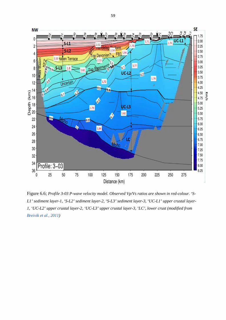
59
Figure 6.6; Profile 3-03 P-wave velocity model. Observed Vp/Vs ratios are shown in red-colour. ‘S-
L1’ sediment layer-1, ‘S-L2’ sediment layer-2, ‘S-L3’ sediment layer-3, ‘UC-L1’ upper crustal layer-
1, ‘UC-L2’ upper crustal layer-2, ‘UC-L3’ upper crustal layer-3, ‘LC’, lower crust (modified from
Breivik et al., 2011)
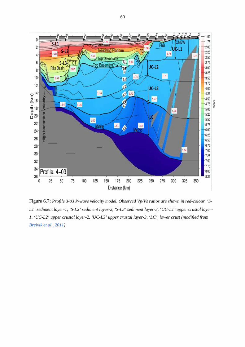
60
Figure 6.7; Profile 3-03 P-wave velocity model. Observed Vp/Vs ratios are shown in red-colour. ‘S-
L1’ sediment layer-1, ‘S-L2’ sediment layer-2, ‘S-L3’ sediment layer-3, ‘UC-L1’ upper crustal layer-
1, ‘UC-L2’ upper crustal layer-2, ‘UC-L3’ upper crustal layer-3, ‘LC’, lower crust (modified from
Breivik et al., 2011)
61
7) Discussion on Results;
Numerous studies show that a good agreement exists between Vp/Vs ratios and subsurface
lithology. (e.g. Picett, 1963; Domenico, 1984; Tatham, 1985; Tatham and McCormac, 1991).
Limestones and sandstones show a low range of Vp/Vs ratio i.e. (1.6-1.75) and (1.84-1.99)
respectively. However, shales are associated with higher Vp/Vs values i.e. 1.70-3.0
(Domenico, 1984). However, above mentioned measurements are very much sensitive to
nature of pore fluid, porosity, its shape and consolidation degree and may vary drastically
upon changing these parameters (Tatham, 1985; Tatham and McCormac, 1991). For example
it has been observed that Vp/Vs ratios could extend upto 10.0 to 16.0 in less consolidated
sediments up to to 50 m below the sea bottom in the Norwegian Sea (Whitmarsh and Miles,
1990). These high values are related to low degree of compaction in sediments (e.g. Chung et
al., 1990; Bromirski et al., 1992). Vp/Vs ratios could be very low in gas filled sandstones i.e.
< 1.60, because low p-wave velocities in such sediments.
7.1) Vp/Vs ratio for the sedimentary layers;
In both profiles the sediment p-wave velocity layering can be divided into 3-distant
categories. The shallower upper layer represented by 2-2.5 km/s p-wave velocities while
second sediment layer can be classified by 3-3.5 km/s p-wave velocity range. Similarly, third
layer with p-wave velocities around 4-5.5 km/sec is shown in the figures 6.6 and 6.7. Velocity
coloring distinguishes them as light pink (1st layer), red (2nd layer) and yellow to green (3rd).
Layer-1;
Due to poor data quality only few arrivals have been interpreted to be constraining Vp/Vs in
this layer and therefore, further resolution is not possible. Average Vp/Vs in this layer is
calculated to be 2.50 along Profile-3 while 2.70 along Profile-4. Variation in these values
along both the profiles can’t be calculated due to limited arrivals, so these Vp/Vs ratios have
been considered as the representative values for this layer.
The relatively high values of Vp/Vs observed are due to poor consolidation of sediments just
below the sea bed. The same trend has been observed by several other studies as well. P.
Digranes et al., 1998 have reported a Vp/Vs value of 2.2-2.4 for the same sediment layer (0-3
km depths) just adjacent to our study area further NW. As the layer thickens to the NW,
slightly lower values could be because of increasing compaction further NW as compared to
our area. As our Vp/Vs values (=2.5 and 2.7) have been calculated near OBS-28 and OBS-39
62
in Profile-3 and 4, therefore it is very much likely that Vp/Vs values decrease to 2.2-2.4 to
NW for this layer. Similarly as Vp/Vs ratios of 3.0 to 5.50 has also been observed in shallow
sediments in Lofoten Continental Margin further north (Kodaira et al, 1996).
Layer-2;
Vp/Vs of 2.40 have been calculated for this layer on Profile 4 close to NW end of the profile.
However this layer is not constrained by arrivals on profile 3. Comparative studies for the
same depths (3-5 km) show an average value of Vp/Vs=2.3 close to Profile-4 and a value of
2.1 close to Profile-3 further NW (Digranes et al, 1998). Therefore, approximately 2.1 or 2.2
Vp/Vs value range can be expected for this layer under Profile-3. However, it should be noted
that values represented by Digranes et al, 1998 are average Vp/Vs values along the whole
length (average length=120 km) of their profiles just further NW from our profiles.
Layer-3;
This layer is present between upper reddish layer and lower top-basement, roughly on both
the profiles. Moderate lateral velocity variations exist in this layer and hence the Vp/Vs ratios.
Profile-3 covers only a portion of Rås Basin and no s-wave arrivals can be mapped from this
basin. However, Profile-4 shows s-wave arrivals under the Rås Basin at about 10-11 km
depth. Since sediment Layer-2 has 2.4 Vp/Vs, so this layer is constrained by Vp/Vs of 1.98.
No comparison can be made further NW because; Rås Basin is localized only in this area. It is
interesting to note that a Vp/Vs of 1.75 is noted immediately further NW from Profile-4 for
the same depths. It is because that Rås Basin is a localized deep basin and represents low-
velocity sediments present at greater depth. However, this trend terminates further NW and is
replaced by upper basement layer with lower Vp/Vs ratios. Therefore, Vp/Vs ratio of 1.98 in
Rås Basin is reasonable because of the sedimentary fill. Depth to top basement is uncertain
along both the profiles. Therefore lower boundaries for the sediment layers can’t be marked
with full certainty.
Similarly as we move NW to SE between 3rd sedimentary layer and top basement another
interesting thing is observed. Along Profile-3, Vp/Vs for 3rd sediment layer have been
averaged to be 1.81 under OBS-29, however towards SE direction, this value changes to 2.13.
Roughly same trend is observed under Profile-4 where Vp/Vs of 1.98 under Rås Basin
changes to 2.02 under the Dønna terrace with further increase to 2.34 as we move more
63
towards the SE direction. It could be justified by the fact that decreasing burial depths causes
metamorphic grades getting lower, thus increasing Vp/Vs.
Central Norway Basement window (CNBW) is exposed along the S-eastern tip of Profiles. A
significant decrease in p-wave velocities is observed under OBS25 and 26 along Profile-3.
Breivik et al, 2011 concluded that it could represent a Devonian detachment transporting
Devonian strata to NW. From here on top basement lies under Devonian strata. This
assumption could be supported by sharp Vp/Vs changes along this transition. Being 1.70 SE
and 1.94 towards the NW side i.e. transition from lower Poisson ratio to higher indicate
change of lithology.
7.2) Vp/Vs ratio for basement and Moho;
Profile-3 and 4 show that basement is heterogeneous and is composed of different distinctive
velocity layers (Breivik et al, 2011). For interpretational purpose we can name it as Upper and
lower crust. Upper crust is further classified into three distinctive layers i.e. Layer-1, 2, and 3
as shown in figures 6.6 and 6.7.
Upper Crust;
Upper crustal Layer-1 is exposed on the SE side of both profiles as CNBW. However, after
OBS-35 on P-rofile 4 and OBS-25 on Profile-3, Devonian detachment results in placement of
Devonian strata on it. From here, only two upper crustal layers can be identified (Breivik et al.
2011).
Upper Crust along with lower crust represents dominant p to s-conversion interfaces and most
of the arrivals which travel to land stations from NW to SE direction are being converted at
upper crustal level.
Its layer-1 (CNBW) present on SE side has an average Vp/Vs ratio of 1.72 on both of the
profiles. Its 2nd and 3rd layers which extend all along both profiles have average Vp/Vs of
1.76 on Profile-4. Studies adjacent to our profiles in NW direction suggest Vp/Vs=1.75 for
these layers (P. Digranes et al. 1998). Similarly, values obtained under Profile-4 are also in
agreement with those measured further north in Lofoten area i.e. 1.73 (Mjelde and Sellevoll,
1993). Holbrook et al, 1992 concluded that average Vp/Vs values in continental crust are
close to 1.73. By keeping in view the uncertainty associated with the picks i.e. 150-200ms, it
can be concluded that Vp/Vs ratio of 1.76 agrees with this on Profile-3 and 4.
64
Similarly Vp/Vs measured for upper crust along Profile-3 does show deviation from what
measured along Profile-4. Profile-4 does not have so much lateral and vertical velocity
variations in the upper crust as compared to Profile-3. Therefore, Vp/Vs show more variations
along Profile-3 for this layer. P-wave velocities are higher in Layer-3 than in Layer-2 under
Profile-3 as compared to velocities under Profile-4 which have comparable velocities in both
layers. Layer-2 shows variation of Vp/Vs to 1.72 at NW to 1.78 towards SE. Similarly, Layer-
3 also shows the same trend having 1.79 values of Vp/Vs on right side and 1.82 to the left.
The average Vp/Vs values measured adjacent to the Profile-3 further NW differ slightly, i.e.
1.75.
Lower-crust;
Along Profile-4 Vp/Vs of 1.83 is observed at the top of bulge in Moho under OBS-35. It
varies slightly to 1.80 under OBS-39 and 1.84 under OBS-45. Therefore, Vp/Vs of 1.82
represent average value for lower crust. Studies close to Profile-4 in NW-direction do show
Vp/Vs of 1.80 for the lower crust (P. Digranes et al. 1998). Similarly, It is evident that Vp/Vs
for lower crust are significantly higher than the 1.75 in upper crust.
Laboratory measurements of oceanic basalts show a Vp/Vs ratio of 1.86-2.04 (Hamilton,
1979) while measurement on gabbro indicated a Vp/Vs ratio of 1.77-1.90 (Holbrook et al,
1992). Upper, middle and lower oceanic crustal measurements at the Lofoten margin reveal
Vp/Vs ratios of 1.86, 1.76 and 1.80 respectively (Kodaira et al, 1996). A Vp/Vs ratio close to
1.90 has been calculated at the continent-ocean transition in the same area (Mjelde et al,
1996b). Similarly Vp/Vs ratio of 1.88 has also been calculated at the Green-margin (Chian
and Louden, 1994).
The lower crust in the outer Vøring area has been supposed to be magmatic under-plated body
which was created before the opening of Norway and Greenland, source to which was Iceland
hot spot as discussed by Skogseid et al, 1992 and Eldholm and Grue, 1994. However, in our
case no evidence of magmatic under-plating can be found.
7.3) Lithological Interpretation;
Profile-4
For Profile-4, along the three upper crustal layers the average Vp, Vp/Vs and σ values are
presented below,
65
Upper-crust, Layer-1; Vp=6.03 km/s, Vp/Vs=1.72 and σ=0.245
Upper-crust, Layer-2; Vp=6.15 km/s, Vp/Vs=1.73 and σ=0.250
Upper-crust, Layer-3; Vp=6.28 km/s, Vp/Vs=1.747 and σ=0.26
The ranges in Vp, Vp/Vs and σ suggest that composition of upper crust to be Granitic (Birch,
1961, Holbrook et, al, 1987 Holbrook et al, 1988, Christensen, 1988). It is difficult to estimate
the exact mineralogical composition responsible for Poisson ratios for the layers. However,
average 0.255 Poisson ratio value show higher quartz content in the upper crust. Similarly
slight increase in Poisson ratio with depth represent decreasing quartz content in the upper
basement layers.
For lower crust the value for different parameters are Vp=6.7-6.8 km/s, Vp/Vs=1.82 and
σ=0.285-0.29. Therefore an increase in Poisson ratio is observed from the upper crust to the
lower one. This increase is probably attributed to the more quartz-poor mafic composition of
the lower crust. Granulite rocks represent the most favorable candidate for the lower crust.
These might include intermediate-mafic to mafic rocks i.e. anorthosite, pyroxene and
hornblende Granulitic facies. However, it is difficult to state about the exact lithology of the
lower crust (Holbrook et, al, 1987 Holbrook et al, 1988, Christensen, 1988)
Similarly, lateral variations in Poisson ratio are also observed in the lower crust. For e.g.
under OBS-36 different parameters are, Vp=6.82 km/s, Vp/Vs=1.83 and σ=0.29 while for
OBS-40 above values are Vp=6.7 km/s, Vp/Vs=1.80 and σ=0.275. Probably, such lateral
changes are probably related to changes in quartz content. Poisson values σ=0.275 show more
quartz content (>10%) than σ=0.29 as discussed by Holbrook et, al, 1987 Holbrook et al,
1988.
Profile-3
For Profile-3, along the three upper crustal layers the average Vp, Vp/Vs and σ values are
given below,
Upper-crust, Layer-1; Vp=5.90 km/s, Vp/Vs=1.73 and σ=0.25
Upper-crust, Layer-2; Vp=6.28 km/s, Vp/Vs=1.74 and σ=0.267
Upper-crust, Layer-3; Vp=6.62 km/s, Vp/Vs=1.80 and σ=0.273
66
Similar to Profile-4, the range of above parameters show that Upper-crust is composed of
quartz-rich Granitic rocks under Profile-3. However, here the average σ values for crustal
layers are bit higher than for the Profile-4. It probably suggests slightly more quartz rich
granitic rocks under Profile-3 as compared to Profile-4. Just like Profile-4 decreasing quartz
content is observed in the successively deeper upper-crustal layers. This decrease is shown by
increasing average Poisson ratio values for deeper layers.
In case of lower crust the seismic parameters derived are,
Lower-crust; Vp=6.94 km/s, Vp/Vs=1.84 and σ=0.285.
Along Profile-3 lower crust is thinner as compared to Profile-4. The Poisson value of 0.285
shows that it has similar composition like the lower-crust along Profile-4. In case of Profile-4,
lateral variations in Poisson ratios were observed. However, due to poor quality coverage of
the lower-crust along Profile-3 only one Poisson ratio value can be calculated.
67
8) Conclusions;
• A relatively low quality shear wave data has been recorded on three-component Ocean
Bottom Seismometers (OBS) and accompanying Land Stations along the Profiles 3-03
and 4-03. Shear-wave modeling has been performed by using already generated p-
wave models utilizing 2-D kinematic ray-tracing. All of the observed s-wave arrivals
have been interpreted and modeled to be P to S-conversions at various velocity
interface and subjected to mode conversion only once along their ray-path.
• For shallower sediments (1-6 km depths) relatively higher Vp/Vs ratios have been
observed i.e. 2.0-2.6. Higher values show the presence of unconsolidated sediments.
For deeper sediments (6-11 km depth) present north-western parts of the profiles,
Vp/Vs ratios decrease to 1.8-2.0 km. This reduction in Vp/Vs ratio is an indicative of
higher compaction in the lower sediments as compared to the upper ones.
• High velocity basement layers act as dominant conversion interfaces especially for
those stations which are closer to the land and significantly higher P to S-wave
converted energy is observed for greater angle of incidences along basement layers.
For upper crust the mean Vp/Vs ratio of 1.75-1.78 indicates its continental origin.
• Upper-crust is composed of quartz-rich granitic rocks under both the profiles.
However, the percentage of quartz decreases with depth and mafic character increases.
• The high average Vp/Vs ratios (Vp/Vs=1.84) for lower crust along both the profiles
show that it is composed of intermediate-mafic to mafic constituents.
68
References
Andersen, T. B., Jamtveit, B., Dewey, J. F., & Swensson, E. (1991). Subduction and eduction
of continental crust: major mechanisms during continent-continent collision and orogenic
extensional collapse, a model based on the south Norwegian Caledonides. Terra Nova, 3(3),
303-310.
Anstey, Nigel Allister. Seismic Interpretation: The Physical Aspects: Being a Record of the
Short Course, the New Seismic Interpreter. International Human Resources Development
Corporation, 1977.
Beaumont, Christopher, Charlotte E. Keen, and Ross Boutilier. "On the evolution of rifted
continental margins: comparison of models and observations for the Nova Scotian margin."
Geophysical Journal International 70.3 (1982): 667-715.
Bering, D. "The orientation of minor fault plane striae and the associated deviatoric stress
tensor as a key to the fault geometry in part of the More–Trondelag fault zone, on-shore
central Norway." Structural and Tectonic Modelling and its Application to Petroleum
Geology. Norwegian Petroleum Society (NPF), Special Publications 1 (1992): 83-90.
Bevington, Philip R., and D. Keith Robinson. Data reduction and error analysis for the
physical sciences. Vol. 2. New York: McGraw-Hill, 1969.
Birch, Francis. "The velocity of compressional waves in rocks to 10 kilobars: 2." Journal of
Geophysical Research 66.7 (1961): 2199-2224.
Blystad, P., Brekke, H., Færsethf, R.B., Skogseid, J. & Tørudbakken, B. 1995. Structural
elements of the Norwegian continental shelf. Part II: The Norwegian Sea Region. NPD-
Bulletin No. 8, the Norwegian Petroleum Directorate, 45.
Bott, M. H. P. "Crustal doming and the mechanism of continental rifting." Tectonophysics
73.1 (1981): 1-8.
Breivik, A. J., Mjelde, R., Raum, T., Faleide, J. I., Murai, Y., & Flueh, E. R. (2011). Crustal
structure beneath the Trøndelag Platform and adjacent areas of the mid--Norwegian margin,
as derived from wide-angle seismic and potential field data. Norwegian Journal of Geology,
90, 141-161.
69
Brekke, Harald, and Frldtjof Riis. "Tectonics and basin evolution of the Norwegian shelf
between 62oN and 72oN." Norsk Geologisk Tidsskrift 67.4 (1987): 295-321.
Brekke, Harald. "The tectonic evolution of the Norwegian Sea continental margin, with
emphasis on the Voring and More basins." Special Publication-Geological Society of London
167 (2000): 327-378.
Bromirski, P.D., Frazer, L.N., Dunnebier, F.K., 1992. Sediment shear Q from airgun OBS
data. Geophys. J. Int. 110, 465–485.
Bukovics, C., Cartier, E. G., Shaw, N. D., and Ziegler, P. A. (1984). Structure and
development of the mid-Norway continental margin. In Petroleum geology of the North
European margin (pp. 407-423). Springer Netherlands.
Bukovics, Christian, and Peter A. Ziegler. "Tectonic development of the Mid-Norway
continental margin." Marine and Petroleum Geology 2.1 (1985): 2-22.
Cassell. B.R., 1982, A method for calculating synthetic seismograms in laterally varying
media: Geophys. J. Roy. Astr. SK 69, 339.354
Červený V., Pšenčík L., 1981. 2-D seismic ray package. Res. Rep., Institute of Geophysics,
Charles University, Prague.
Cerveny, V., I. A. Molotkov, and I. Psencik (1977). Ray Method in Seismology, Charles
Univ. Press, Prague.
Chian, Deping, and Keith E. Louden. "The continent-ocean crustal transition across the
Southwest Greenland Margin." Journal of Geophysical Research: Solid Earth (1978–2012)
99.B5 (1994): 9117-9135.
Christensen, N. 1. Poisson‘s ratio and Crustal Seismology, Journal of Geophysical Research,
Vol. 101, No. B2, Pages 3139-3156, February 10, 1996
Chung, T.W., Hirata, N., Sato, R., 1990. Two-dimensional P- and S-wave velocity structure
of the Yamato Basin, the southern Japan sea, from refraction data collected by an ocean
bottom seismographic array. J. Phys. Earth 38, 99–147.
Daley P.F., Krebes E.S. (2004). SH wave propagation in viscoelastic media. Studia
Geophysica et Geodaetica 48, 563-587.
70
Dewey, John F. "Plate tectonics and the evolution of the British Isles Thirty-fifth William
Smith Lecture." Journal of the Geological Society 139.4 (1982): 371-412.
Digranes, P., Mjelde, R., Kodaira, S., Shimamura, H., Kanazawa, T., Shiobara, H., & Berg, E.
W. (1998). A regional shear-wave velocity model in the central Vøring Basin, N. Norway,
using three-component Ocean Bottom Seismographs. Tectonophysics, 293(3), 157-174.
Domenico, S.N., 1984. Rock lithology and porosity determination from shear and
compressional wave velocity. Geophysics 49, 1188–1195.
Doré, A. G., and E. R. Lundin. "Cenozoic compressional structures on the NE Atlantic
margin; nature, origin and potential significance for hydrocarbon exploration." Petroleum
Geoscience 2.4 (1996): 299-311.
Edwin S. Robinson, Cahit Çoruh, Basic exploration geophysics, ISBN 047187941X,
9780471879411, Wiley, 1988, p#15-22.
Eldholm, O and Coffin, MF, Large Igneous Provinces and Plate Tectonics, History and
Dynamics of Global Plate Motions, American Geophysical Union, MA Richards, RG Gordon,
RD Van Der Hilst (ed), Washington DC, pp. 309-326. ISBN 0-87590-979-5 (2000)
Eldholm, O., Grue, K., 1994. North Atlantic volcanic margins: Dimensions and production
rates. J. Geophys. Res. 99, 2955–2968.
Fossen, Haakon. "Extensional tectonics in the Caledonides: Synorogenic or postorogenic?."
Tectonics 19.2 (2000): 213-224.
Foucher, J. P., Le Pichon, X., Sibuet, J. C., Roberts, D. G., Chenet, P. Y., Bally, A. W., ... &
Turcotte, D. L. (1982). The Ocean--Continent Transition in the Uniform Lithospheric
Stretching Model: Role of Partial Melting in the Mantle [and Discussion]. Philosophical
Transactions of the Royal Society of London. Series A, Mathematical and Physical Sciences,
305(1489), 27-43.
Gabrielsen, R. H., Foerseth, R., Hamar, G., & Rønnevik, H. (1984). Nomenclature of the main
structural features on the Norwegian Continental Shelf north of the 62nd parallel. In
Petroleum Geology of the North European Margin (pp. 41-60). Springer Netherlands.
71
Gabrielsen, Roy H., Rune Kyrkjebø, Jan Inge Faleide, Willy Fjeldskaar, and Tomas
Kjennerud. "The Cretaceous post-rift basin configuration of the northern North Sea."
Petroleum Geoscience 7, no. 2 (2001): 137-154.
Gaiser, James E. "Compensating OBC data for variations in geophone coupling." 1998, SEG
Annual Meeting, 1998.
Grønlie, A., et al. "Fission-track and K-Ar dating of tectonic activity in a transect across the
Møre-Trøndelag Fault Zone, central Norway." Norsk Geologisk Tidsskrift 74.1 (1994): 24-34.
Haller, J., Haller, J., Haller, J., Haller, J., & Geologist, S. (1971). Geology of the East
Greenland Caledonides (p. 415). New York: Interscience.
Hamilton, E.L., 1979. Vp=Vs and Poisson’s ratio in marine sediments and rocks. J. Acoust.
Soc. Am. 66, 1093–1101.
Hellinger, Steven J., and John G. Sclater. "Some comments on two-layer extensional models
for the evolution of sedimentary basins." Journal of Geophysical Research: Solid Earth
(1978–2012) 88.B10 (1983): 8251-8269
Holbrook, W. Steven, Dirk Gajewski, and Claus Prodehl. "Shear wave velocity and Poisson's
ratio structure of the upper lithosphere in southwest Germany." Geophysical Research Letters
14.3 (1987): 231-234.
Holbrook, W. Steven, Dirk Gajewski, Anton Krammer, and Claus Prodehl. "An interpretation
of wide-angle compressional and shear wave data in southwest Germany: Poisson's ratio and
petrological implications." Journal of Geophysical Research: Solid Earth (1978–2012) 93, no.
B10 (1988): 12081-12106
Holbrook, W.S., Mooney, W.D., Christensen, N.J., 1992. The seismic velocity structure of the
deep continental crust. In: Fountain, D.M., Arculus, R., Kay, R.W. (Eds.), Continental Lower
Crust. Development in Geotectonics 23, Elsevier, Amsterdam, pp. 1–43.
Julian, B. R. and D. Gubbins (1977). Three dimensional seismic ray tracing, J. Geophys. 43,
95-114.
Kearey, Philip, Michael Brooks, and Ian Hill. An introduction to geophysical exploration.
Wiley-Blackwell, 2009.
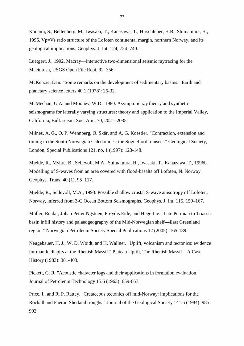
72
Kodaira, S., Bellenberg, M., Iwasaki, T., Kanasawa, T., Hirschleber, H.B., Shimamura, H.,
1996. Vp=Vs ratio structure of the Lofoten continental margin, northern Norway, and its
geological implications. Geophys. J. Int. 124, 724–740.
Luetgert, J., 1992. Macray—interactive two-dimensional seismic raytracing for the
Macintosh, USGS Open File Rept, 92–356.
McKenzie, Dan. "Some remarks on the development of sedimentary basins." Earth and
planetary science letters 40.1 (1978): 25-32.
McMechan, G.A. and Mooney, W.D., 1980. Asymptotic ray theory and synthetic
seismograms for laterally varying structures: theory and application to the Imperial Valley,
California, Bull. seism. Soc. Am., 70, 2021–2035.
Milnes, A. G., O. P. Wennberg, Ø. Skår, and A. G. Koestler. "Contraction, extension and
timing in the South Norwegian Caledonides: the Sognefjord transect." Geological Society,
London, Special Publications 121, no. 1 (1997): 123-148.
Mjelde, R., Myhre, B., Sellevoll, M.A., Shimamura, H., Iwasaki, T., Kanazawa, T., 1996b.
Modelling of S-waves from an area covered with flood-basalts off Lofoten, N. Norway.
Geophys. Trans. 40 (1), 95–117.
Mjelde, R., Sellevoll, M.A., 1993. Possible shallow crustal S-wave anisotropy off Lofoten,
Norway, inferred from 3-C Ocean Bottom Seismographs. Geophys. J. Int. 115, 159–167.
Müller, Reidar, Johan Petter Ngstuen, Frøydis Eide, and Hege Lie. "Late Permian to Triassic
basin infill history and palaeogeography of the Mid-Norwegian shelf—East Greenland
region." Norwegian Petroleum Society Special Publications 12 (2005): 165-189.
Neugebauer, H. J., W. D. Woidt, and H. Wallner. "Uplift, volcanism and tectonics: evidence
for mantle diapirs at the Rhenish Massif." Plateau Uplift, The Rhenish Massif—A Case
History (1983): 381-403.
Pickett, G. R. "Acoustic character logs and their applications in formation evaluation."
Journal of Petroleum Technology 15.6 (1963): 659-667.
Price, I., and R. P. Rattey. "Cretaceous tectonics off mid-Norway: implications for the
Rockall and Faeroe-Shetland troughs." Journal of the Geological Society 141.6 (1984): 985-
992.

73
Robinson, E. S., and C. Coruh. "Basic exploration geophysics Wiley." New Yor-k (1988).
Royden, Leigh, J. G. Sclater, and R. P. Von Herzen. "Continental margin subsidence and heat
flow: important parameters in formation of petroleum hydrocarbons." AAPG Bulletin 64.2
(1980): 173-187.
Skogseid, J., Pedersen, T., Eldholm, O., Larsen, B.T., 1992. Tectonism and magmatism
during NE Atlantic continental break-up: the Vøring margin. In: Story, B.C., Alabaster, T.,
Pankhurst, R.J. (Eds.), Magmatism and the Causes of Continental Breakup. Geol. Soc.
London Spec. Publ. 68, 305–320.
Smelror, Morten, John Dehls, Jörg Ebbing, Eiliv Larsen, Erik R. Lundin, Øystein Nordgulen,
Per Terje Osmundsen et al. "Towards a 4D topographic view of the Norwegian sea margin."
Global and Planetary Change 58, no. 1 (2007): 382-410.
Smythe, D. K., J. A. Chalmers, and A. G. Skuce. "Dobinson. A., and Mould, AS, 1983. Early
opening history of the North Atlantic—I. Structure and origin of the Faroe-Shetland
Escarpment." Geophys. J. R. Astron. Soc 72: 373-398.
Spence, G.D., 1983. RAYAMP: An algorithm for tracing rays and calculating amplitudes in
laterally varying media: program documentation. Univ. of British Columbia.
Spence, G.D., Whittall, K.P. and Clowes, R.M., 1984. Practical synthetic seismograms for
laterally varying media calculated by asymptotic ray theory, Bull. seism. Soc. Am., 74, 1209–
1223
Stein, Seth, and Michael Wysession. An introduction to seismology, earthquakes, and earth
structure. Wiley-Blackwell, 2009. p=55-113.
Surlyk, Finn, S. Piasecki, F. Rolle, L. Stemmerik, E. Thomsen, and P. Wrang. "The Permian
base of East Greenland." In Petroleum geology of the North European margin, pp. 303-315.
Springer Netherlands, 1984.
Svetlov, 1. L., A. 1. Epistian, A. 1. Krivko, A. 1. Samoil, 1. N. Odintsev, and A.P. Andreev,
Anisotropy of Poisson's ratio of single crystals of nickel alloy, Sov. Phys. Dokl., 33, 771-773,
1988.
74
Tatham, R. H., M. D. McCormack, R. H. Tatham, and M. D. McCormack. "3. Rock Physics
Measurements." In Multicomponent Seismology in Petroleum Exploration, edited by E. B.
Neitzel, and D. F. Winterstein, pp. 43-92. Society of Exploration Geophysicists, 1991.
Tatham, R.H., 1985. Shear waves and lithology. In: Dohr, G. (Ed.), Seismic Shear Waves,
Part B. Applications. Geophysical Press, London, pp. 86–133.
Terry, Michael P., Peter Robinson, Michael A. Hamilton, and Michael J. Jercinovic.
"Monazite geochronology of UHP and HP metamorphism, deformation, and exhumation,
Nordøyane, Western Gneiss Region, Norway." American Mineralogist 85, no. 11-12 (2000):
1651-1664.
Turcotte, D. L. "Rifts--tensional failures of the lithosphere." LPI Contributions 457 (1981): 5.
Underhill, J. R. "Jurassic." Petroleum Geology of the North Sea: Basic Concepts and Recent
Advances, Fourth Edition (1998): 245-293.
Whitmarsh, R.B., Miles, P.R., 1990. In situ measurements of shear-wave velocity in ocean
sediments. In: Hovem, J.M., Richardson, M.D., Stoll, R.D. (Eds.), Shear Waves in Marine
Sediments. Kluwer, Dordrecht, pp. 321–328.
Yilmaz, Özdoğan. Seismic data analysis: processing, inversion, and interpretation of seismic
data. No. 10. SEG Books, 2001.
Zelt, C. A. and D. J. White, Crustal structure and tectonics of the southeastern Canadian
Cordillera, J. Geophys. Res., 100, 24255-24273, 1995.
Zelt, C. A. and R. M. Ellis, Practical and efficient ray tracing in two-dimensional media for
rapid travel time and amplitude forward modelling, Can. J. Expl. Geophys., 24, 16-31, 1988.
Zelt, C. A., 3-D velocity structure from simultaneous traveltime inversion of in-line seismic
data along intersecting profiles, Geophys. J. Int., 118, 795-801, 1994.
Zelt, C. A., Modelling strategies and model assessment for wide-angle seismic traveltime
data, Geophys. J. Int., 139, 183-204, 1999.
Ziegler, Peter A. Geological Atlas of Western and Central Europe: 1982. Vol. 1. Geological
Society, 1982.
APPENDIX On the following pages are the data from the OBS and Land-stations, modeled rays and the calculated and observed travel times for each OBS. The arrivals have also been denoted by the naming convention given in Table 6.1 of the thesis.
Appendix consists of seismic data from each OBS & Land stations from Profile-04-03 & 03,
along with traced-rays & observed & calculated times.
Order is…
1. Profile#3
Land-stations starting from SE up to last land-station to NW.
OBS’s starting from SE up to last OBS to NW.
2. Profile#4
Land-stations starting from SE up to last land-station to NW.
OBS’s starting from SE up to last OBS to NW.
PPS14.3
T‐D/4.62 (s)
Horizontal component of Land‐10 with data plo ed in SU and the rays, interpreted and calculated
arrivals from Rayinvr.
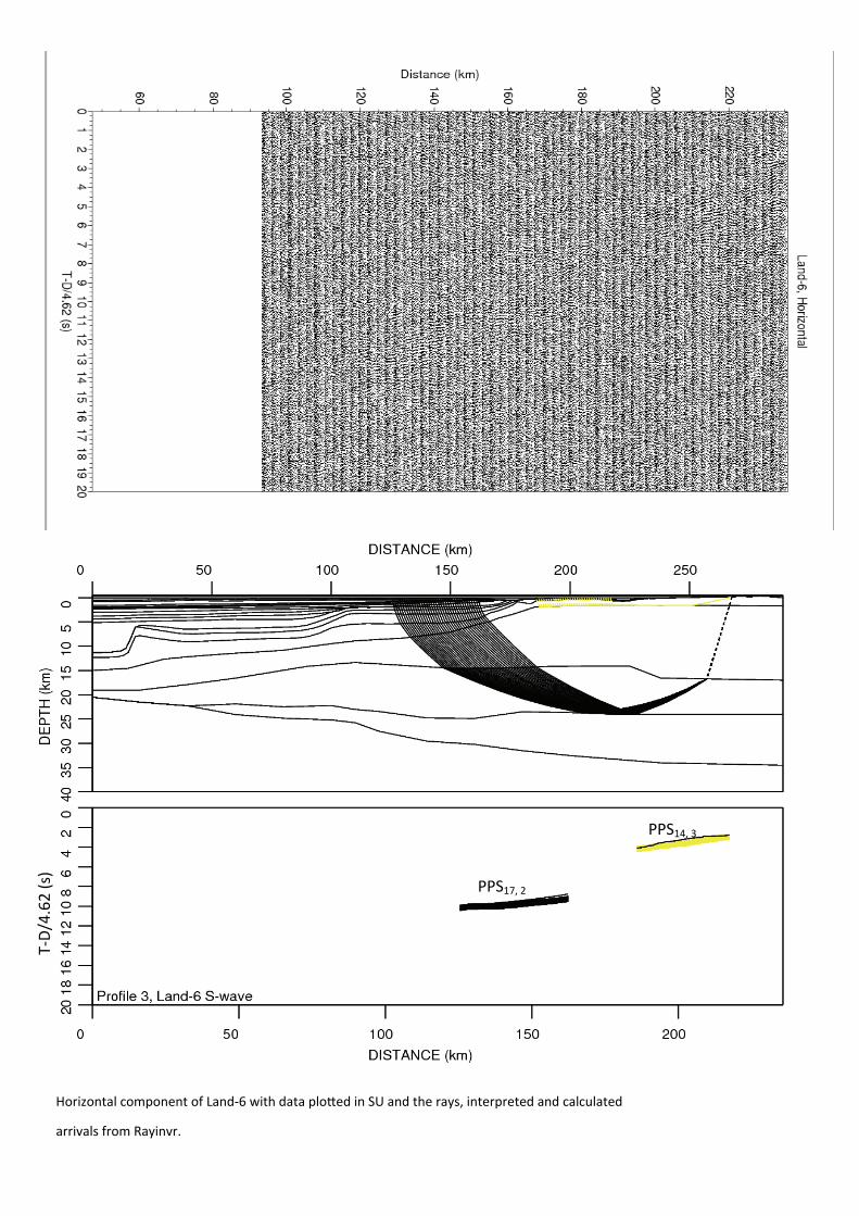
T‐D/4.62 (s)
PPS14, 3
PPS17, 2
T‐D/4.62 (s)
Horizontal component of Land‐6 with data plo ed in SU and the rays, interpreted and calculated
arrivals from Rayinvr.
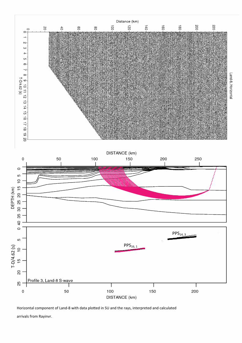
PPS14, 3
T‐D/4.62 (s) PPS16, 1
Horizontal component of Land‐8 with data plo ed in SU and the rays, interpreted and calculated
arrivals from Rayinvr.
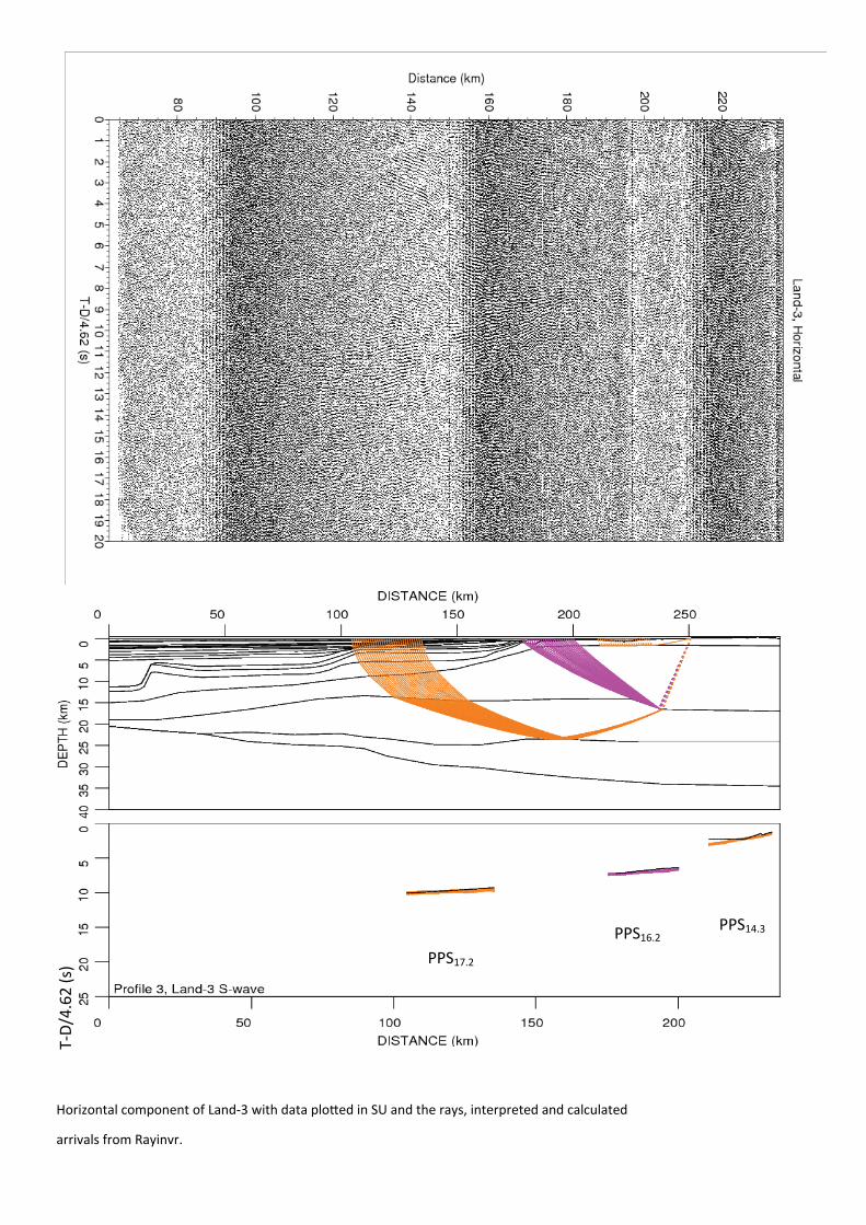
PPS14.3
PPS17.2
PPS16.2
T‐D/4.62 (s)
Horizontal component of Land‐3 with data plo ed in SU and the rays, interpreted and calculated
arrivals from Rayinvr.
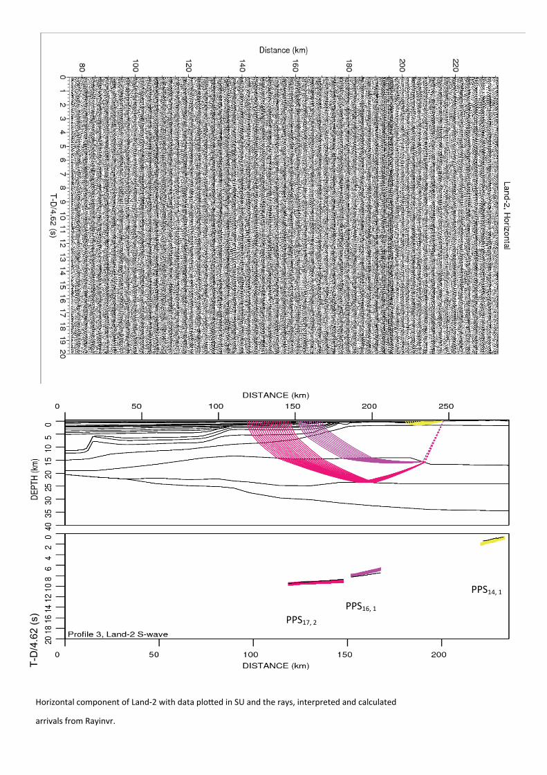
PPS14, 1
PPS17, 2 PPS16, 1
T-D
/4.6
2 (s
)
Horizontal component of Land‐2 with data plo ed in SU and the rays, interpreted and calculated
arrivals from Rayinvr.
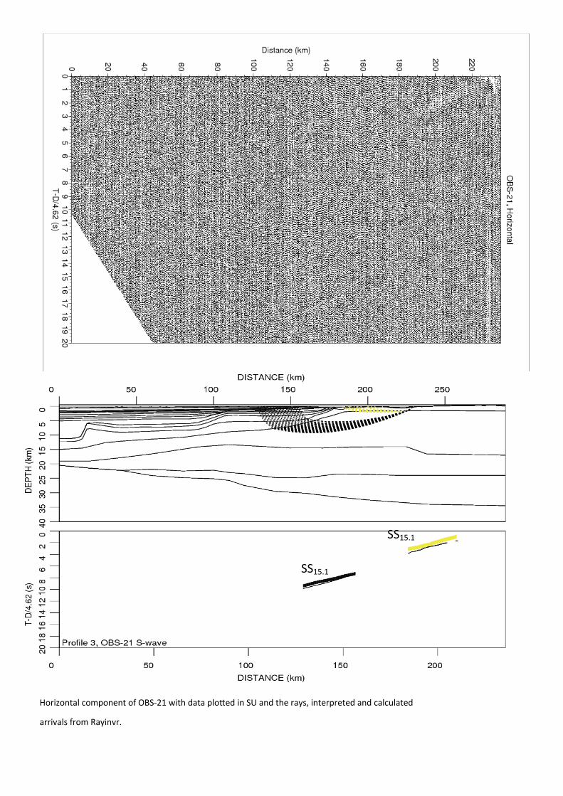
SS15.1
SS15.1
Horizontal component of OBS‐21 with data plo ed in SU and the rays, interpreted and calculated
arrivals from Rayinvr.
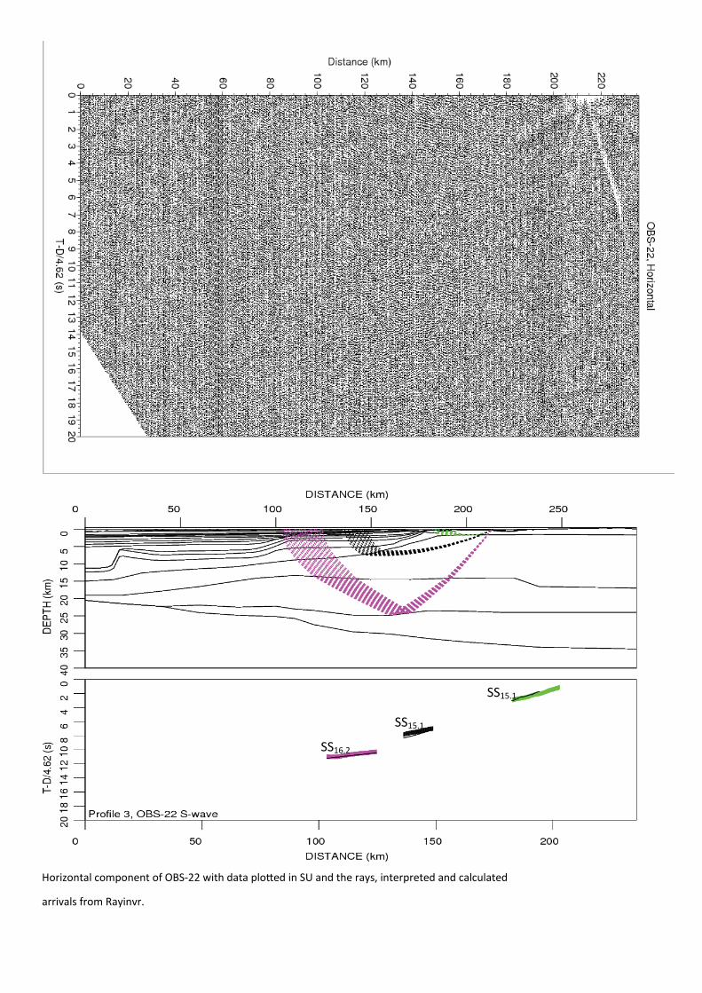
SS15.1
SS15.1
SS16.2
Horizontal component of OBS‐22 with data plo ed in SU and the rays, interpreted and calculated
arrivals from Rayinvr.
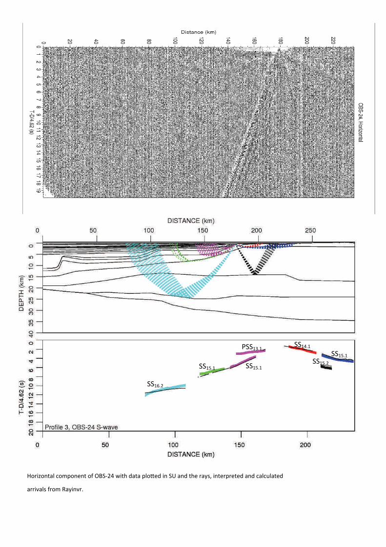
SS15.2 SS15.1
SS14.1 PSS13.1
SS15.1 SS15.1
SS16.2
Horizontal component of OBS‐24 with data plo ed in SU and the rays, interpreted and calculated
arrivals from Rayinvr.
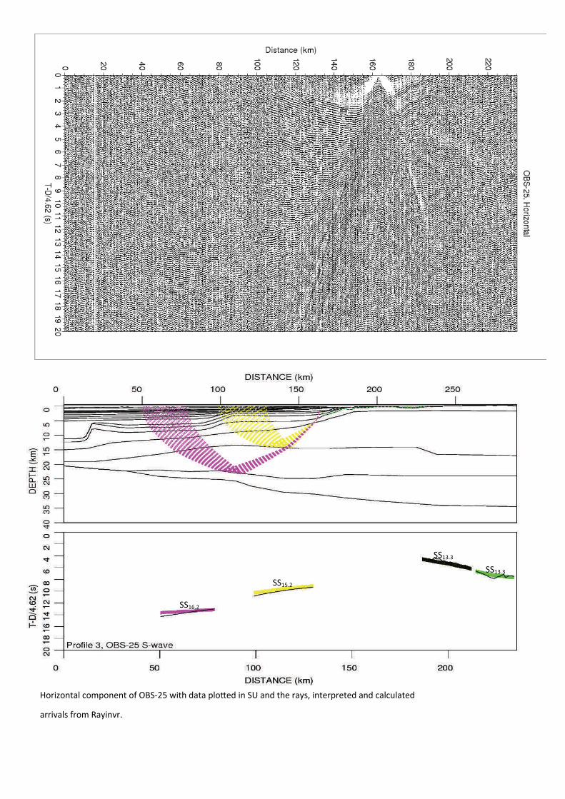
SS13.3
SS13.3
SS16.2
SS15.2
Horizontal component of OBS‐25 with data plo ed in SU and the rays, interpreted and calculated
arrivals from Rayinvr.
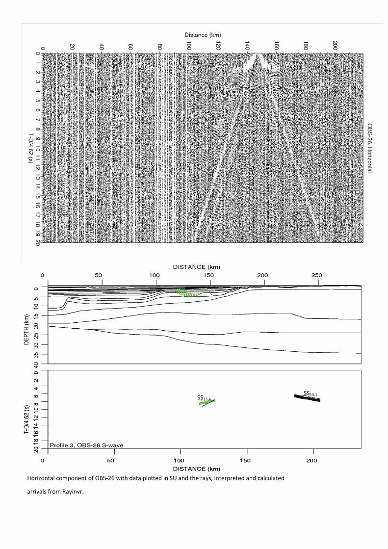
SS13.1 SS13.4
Horizontal component of OBS‐26 with data plo ed in SU and the rays, interpreted and calculated
arrivals from Rayinvr.
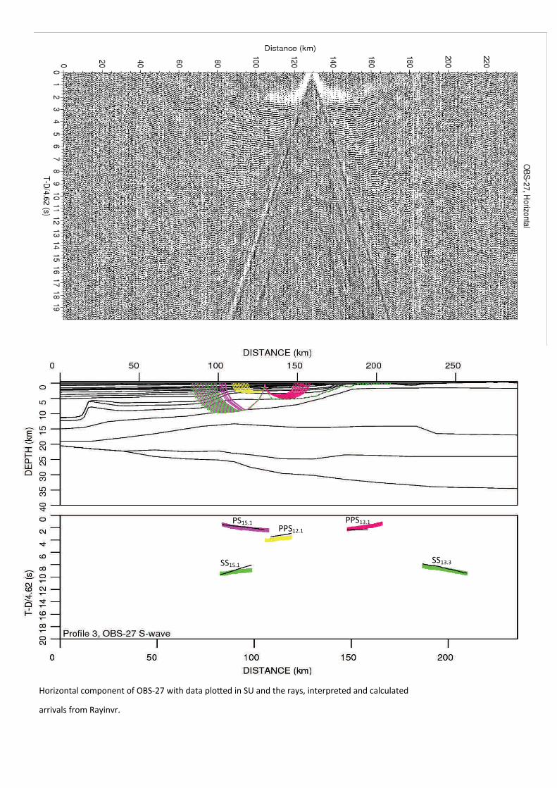
SS13.3 SS15.1
PPS13.1 PPS12.1
PS15.1
Horizontal component of OBS‐27 with data plo ed in SU and the rays, interpreted and calculated
arrivals from Rayinvr.
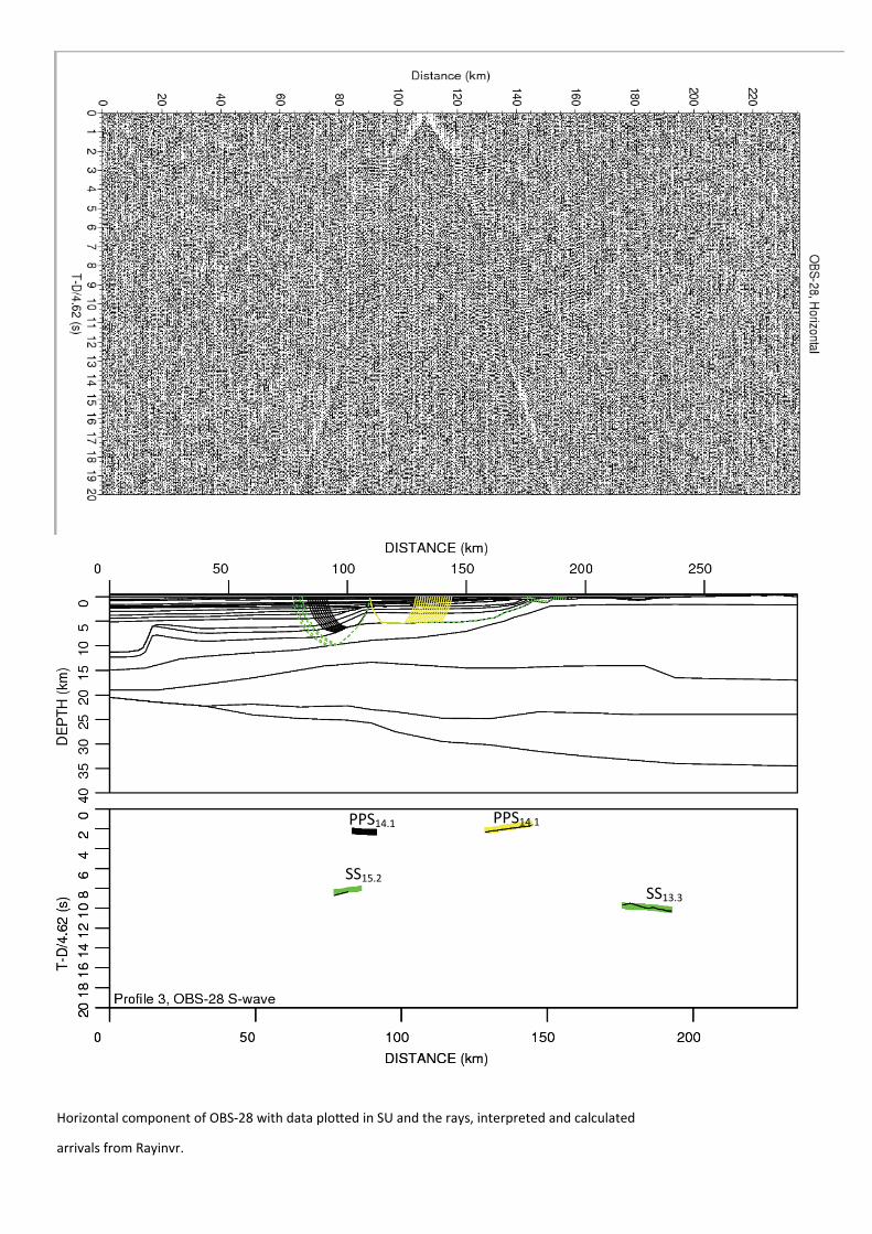
SS13.3
PPS14.1 PPS14.1
SS15.2
Horizontal component of OBS‐28 with data plo ed in SU and the rays, interpreted and calculated
arrivals from Rayinvr.
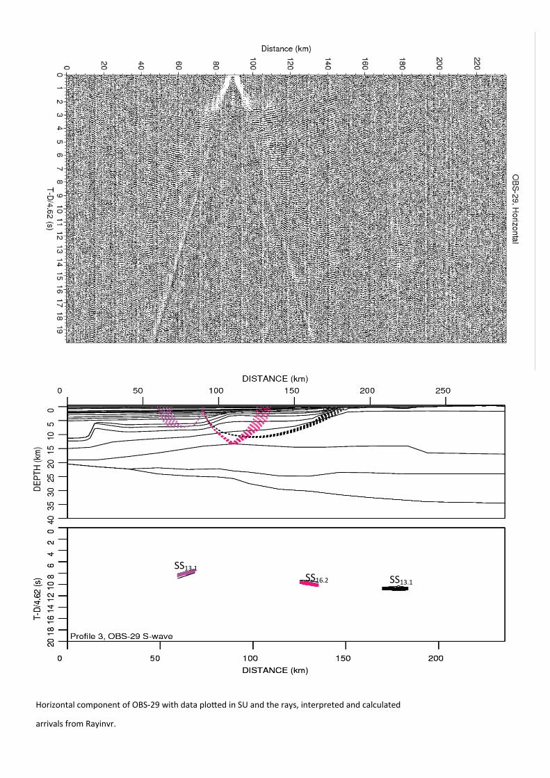
SS13.1 SS16.2 SS13.1
Horizontal component of OBS‐29 with data plo ed in SU and the rays, interpreted and calculated
arrivals from Rayinvr.
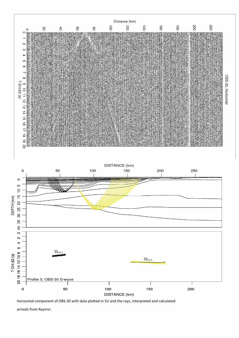
SS17.2
SS14.2
Horizontal component of OBS‐30 with data plo ed in SU and the rays, interpreted and calculated
arrivals from Rayinvr.
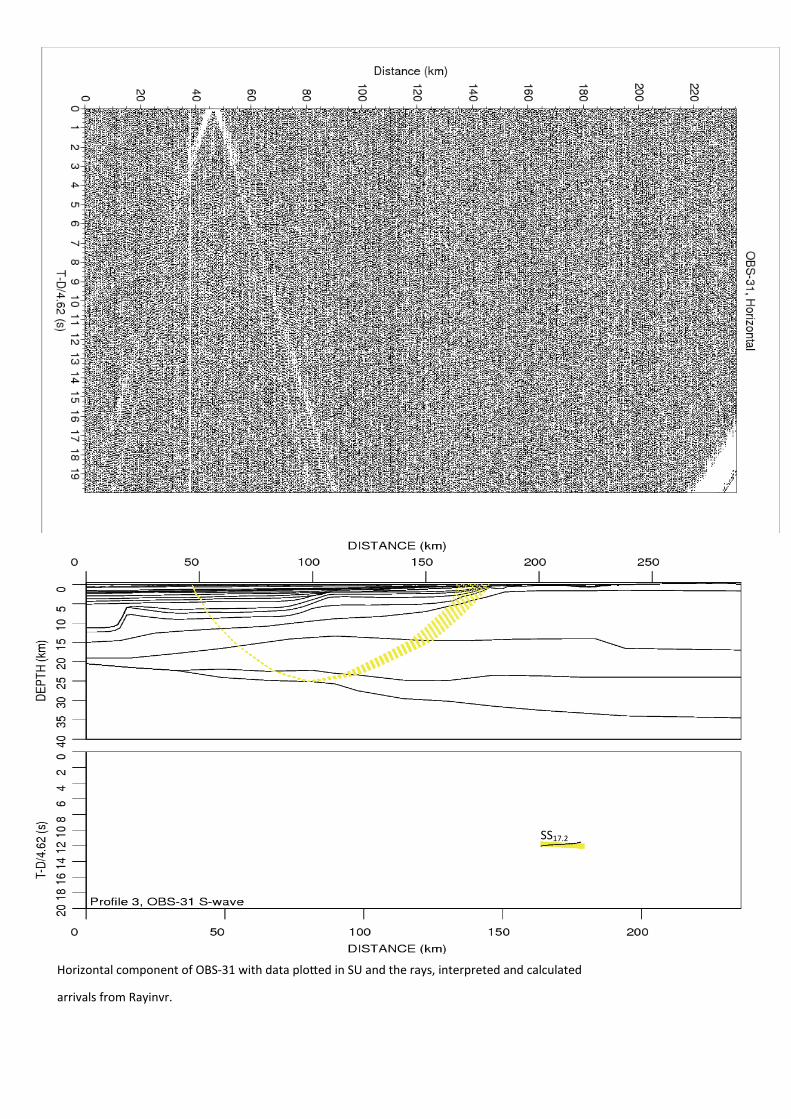
SS17.2
Horizontal component of OBS‐31 with data plo ed in SU and the rays, interpreted and calculated
arrivals from Rayinvr.
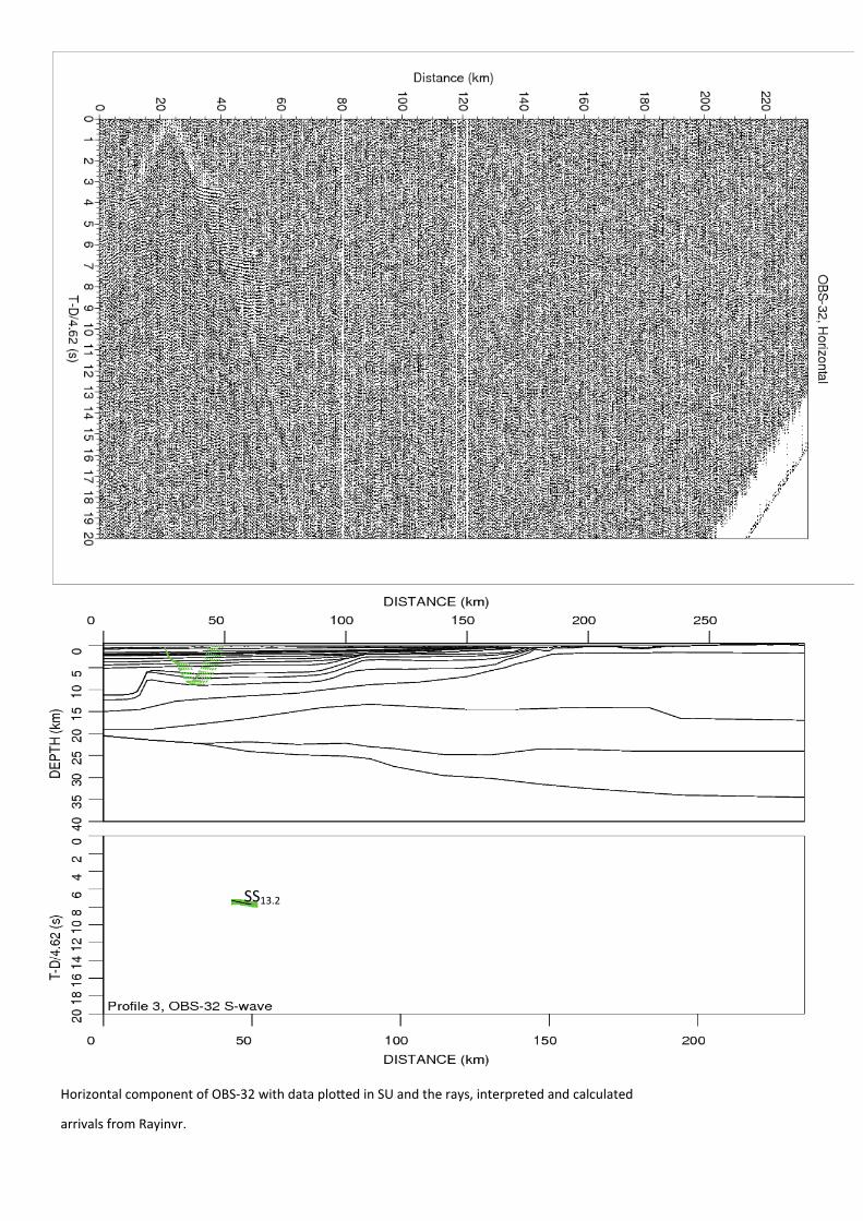
SS13.2
Horizontal component of OBS‐32 with data plo ed in SU and the rays, interpreted and calculated
arrivals from Rayinvr.
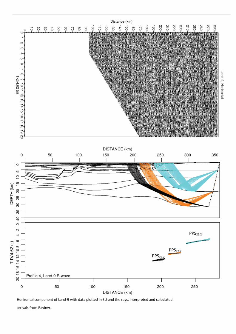
PPS21.2
PPS22.2 PPS22.2
T‐D/4.62 (s)
Horizontal component of Land‐9 with data plo ed in SU and the rays, interpreted and calculated
arrivals from Rayinvr.
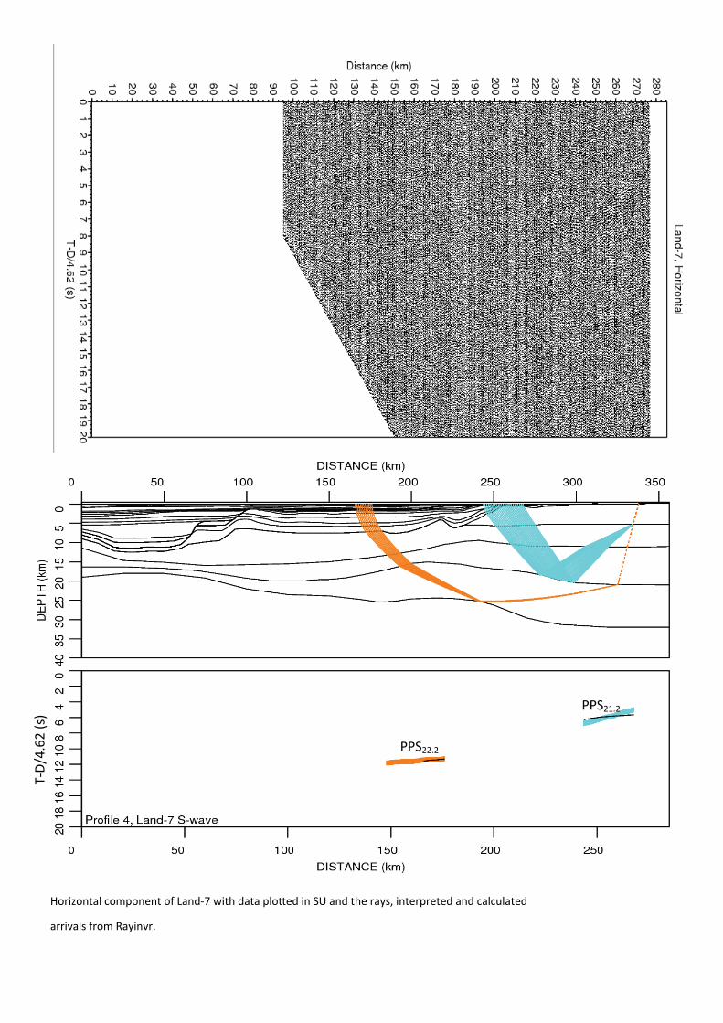
PPS21.2
PPS22.2
T‐D/4.62 (s)
Horizontal component of Land‐7 with data plo ed in SU and the rays, interpreted and calculated
arrivals from Rayinvr.
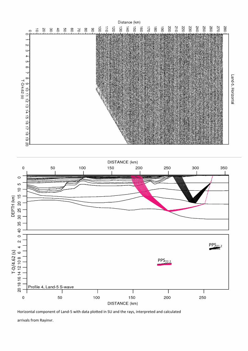
PPS21.2
PPS22.2
T‐D/4.62 (s)
Horizontal component of Land‐5 with data plo ed in SU and the rays, interpreted and calculated
arrivals from Rayinvr.
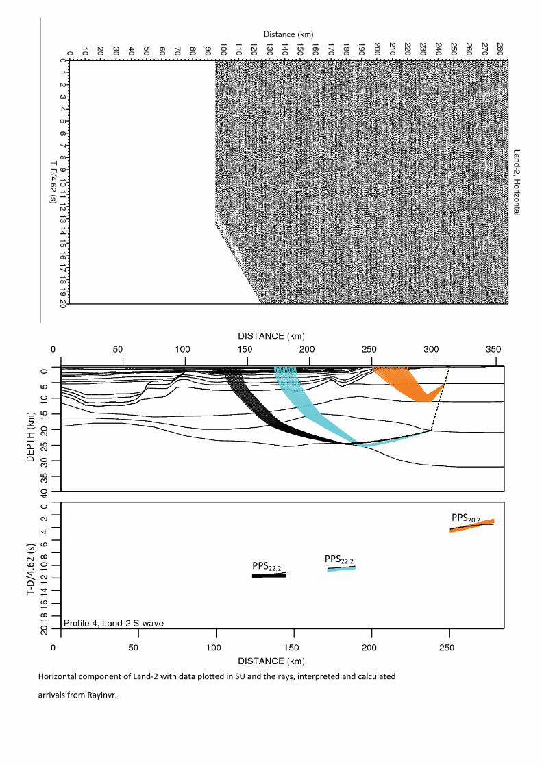
PPS20.2
PPS22.2 PPS22.2
T‐D/4.62 (s)
Horizontal component of Land‐2 with data plo ed in SU and the rays, interpreted and calculated
arrivals from Rayinvr.
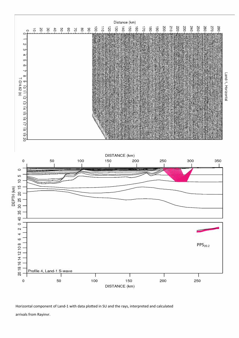
PPS20.2
Horizontal component of Land‐1 with data plo ed in SU and the rays, interpreted and calculated
arrivals from Rayinvr.
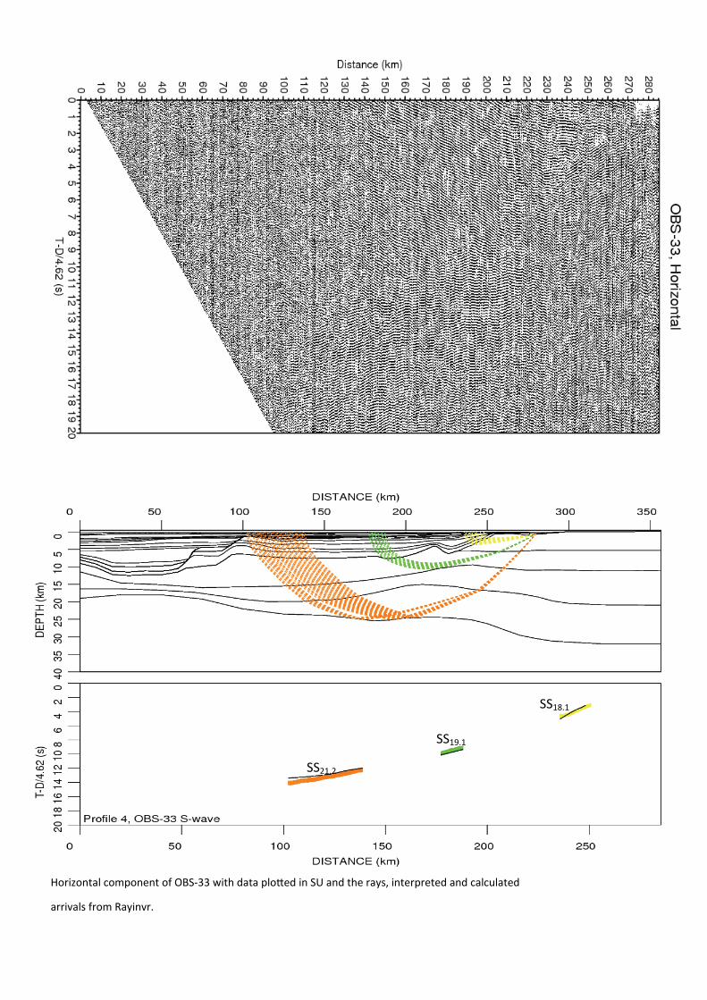
SS18.1
SS21.2
SS19.1
Horizontal component of OBS‐33 with data plo ed in SU and the rays, interpreted and calculated
arrivals from Rayinvr.
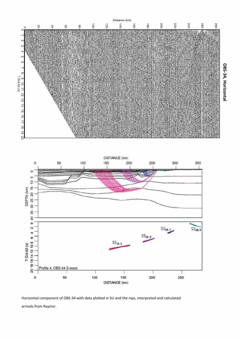
Horizontal component of OBS‐34 with data plo ed in SU and the rays, interpreted and calculated
arrivals from Rayinvr.
OBS‐3
4, H
orizo
ntal
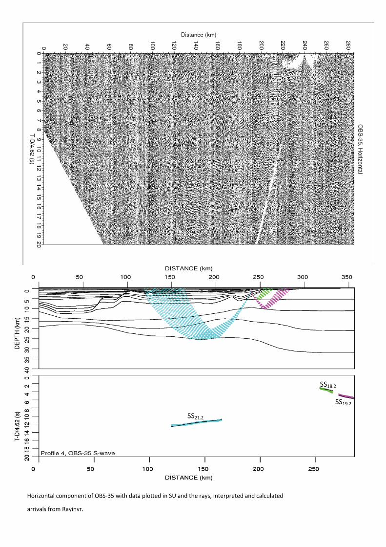
SS21.2
SS19.2
SS18.2
Horizontal component of OBS‐35 with data plo ed in SU and the rays, interpreted and calculated
arrivals from Rayinvr.
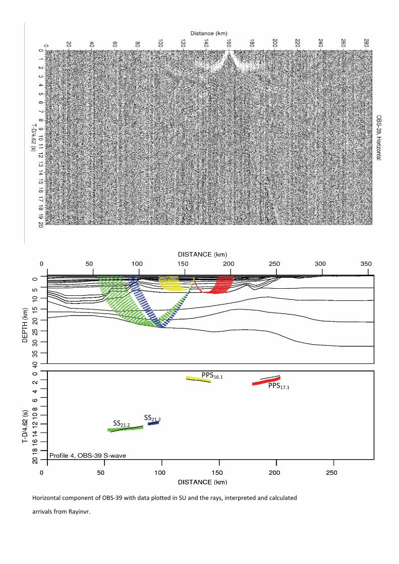
SS21.2 SS21.2
PPS16.1
PPS17.1
Horizontal component of OBS‐39 with data plo ed in SU and the rays, interpreted and calculated
arrivals from Rayinvr.
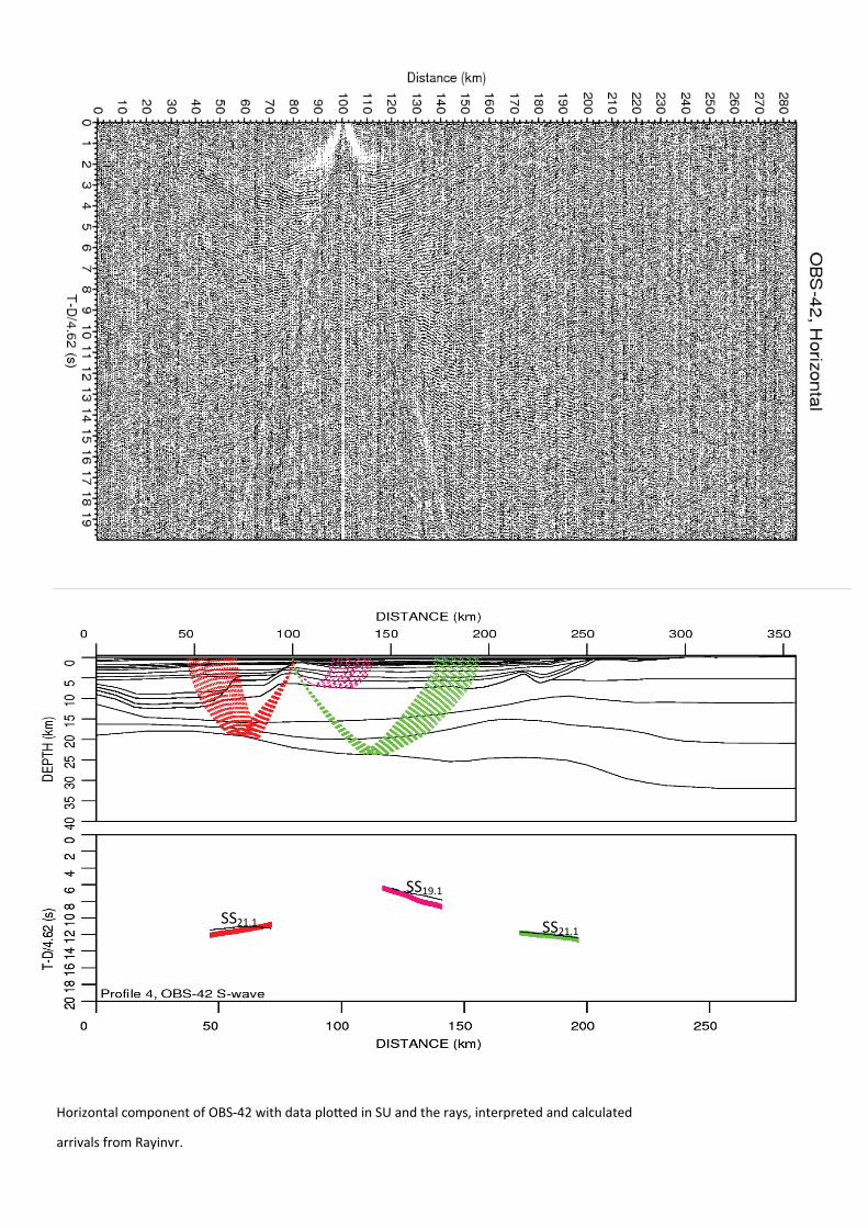
SS19.1
SS21.1 SS21.1
Horizontal component of OBS‐42 with data plo ed in SU and the rays, interpreted and calculated
arrivals from Rayinvr.
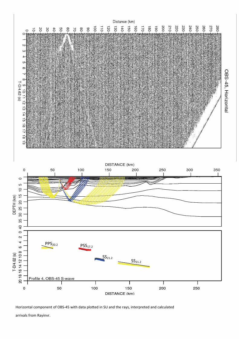
SS21.2 SS21.2
PPS20.2 PSS17.2
Horizontal component of OBS‐45 with data plo ed in SU and the rays, interpreted and calculated
arrivals from Rayinvr.
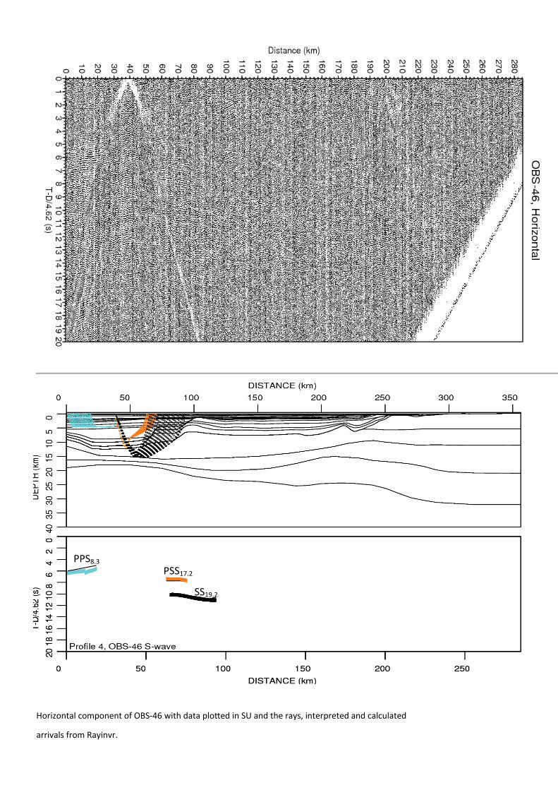
PPS8.3 PSS17.2
SS19.2
Horizontal component of OBS‐46 with data plo ed in SU and the rays, interpreted and calculated
arrivals from Rayinvr.