PSYCHOMETRIKA--VOL. 22, NO. 4 DECEMBER, 1957

T H E USE OF C O N F I G U R A L ANALYSIS FOR T H E EVALUATION OF T E S T SCORING M E T H O D S *

H. G. OSBUR~

SOUTHERN ILLINOIS UNIVERSITY

AND

A R D I E L U B I N

WALTER REED ARMY INSTITUTE OF RESEARCH

A method based on configural analysis has been given whereby test scoring techniques can be evaluated to see if they have optimal validity. Configural analysis has also been used to show how three well known item scoring techniques, multiple regression, total score, and multiple cut-off, imply (for optimal validity) certain conditions on the answer pattern means. The method is illustrated by a worked example.

The purpose of this article is to demonstrate a method whereby test scoring techniques can be evaluated to see if they have maximum validity. In a previous paper [3] a technique of pat tern scoring of test items for the prediction of a quanti tat ive criterion was presented. The basic notion used was tha t of a configural scale, defined as follows: given a test of t items and a quanti tat ive criterion, form all possible answer patterns and assign to each subject a score which is the mean criterion score for all subjects in his answer pattern. This set of scores is called a configural scale. I t was shown that , in the analysis sample, of all possible ways of scoring the t items, the configural scale provides the best least squares prediction of the criterion. I t was fur ther shown tha t the configural scale could be represented exactly by a polynomial function of the i tem scores if the items are dichotomous. However, the concept of the configural scale is not restricted to dichotomous items. If the items are polychotomous, the only change is tha t the number of possible answer pat terns will increase.

Theory A. The equav model

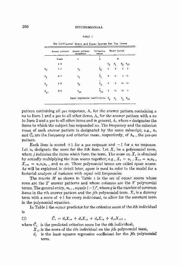
The configural scale is defined as the set of answer pat tern means, and can be represented by a polynomial function of the item scores. An example of the configural scale and polynomial equation for two items is given in T a b l e l . In Table 1 the answer patterns are designated by Ao for the answer

*We are indebted to Professor James G. Taylor for his helpful suggestions.

359

360

A 0

A 1

A 2

AI2

P S Y C H O M E T R I K A

TABLE !

The Cdnfisural Scale and Equa~ Scores f o r Two Items

Answer pattern Answer pattern Criterion Equav scores frequency means

I terns n C

I 2 X 0 X l X 2 X12

Y Y no CO I I I 1

N Y n I C1 I -I 1 -I

Y N n 2 C 2 1 1 -i -I

N N n12 C12 1 -i -i I

Equav regression coefficients d 0 d I d 2 d12

pattern containing all yes responses, A1 for the answer pattern containing a no to Item 1 and a yes to all other items, A2 for the answer pattern with a no

to Item 2 and a yes to all other items and in general, A~ where r designates the items to which the subject has responded no. The frequency and the criterion mean of each answer pattern is designated by the same subscript; e.g., no

and Co are the frequency and criterion mean, respectively, of Ao, the yes-yes

pattern. Each item is scored -{-1 for a yes response and - 1 for a no response.

Let uk designate the score for the kth item. Let Xi be a polynomial term, where ] indicates the items which form the term. The score on Xi is obtained by actually multiplying the item scores together; e.g., X I = u ~ , X12 = u~u2,

X123 = u~u2u3 , and so on. These polynomial terms are called equav scores. As will be explained in detail later, equav is used to refer to the model for a factorial analysis of variance with equal cell frequencies.

The matrix M as shown in Table 1 is the set of equav scores whose rows are t h e 2 t answer patterns and whose columns are the 2 t polynomial terms. The general entry, m r s , equals (-- 1) ~, where g is the number of common items in the rth answer pattern and the jth polynomial term. Xo is a dummy term with a score of + 1 for every individual, to allow for the constant term in the polynomial equation.

In Table I the equav predictor for the criterion score of the ith individual is

(1) O, = doX,o + d~X,1 --[- d~X,2 + d,2X, ,~ ,

where ~ is the predicted criterion score for the ith individual, X . is the score of the ith individual on the ]th polynomial term, d~ is the least squares regression coefficient for the jth polynomial

term.

H . G. OSBURN AND ARDIE LUBIN 361

The exact solution for the 2 t regression coefficients can be obtained as follows. Let Z be an N by 2 * matrix whose general element z~; is the equav score of the i th individual on the j th polynomial term. Z is an expanded form of M where the r th row of M is repeated n, times. Let C be an N-rowed column vector, where c~ is the criterion score of the i th individual. Let d be the 2 ~ X 1 column vector of regression coefficients. Then

(2) d = ( Z ' Z ) - ' Z ' C

is the set of regression coefficients which gives the exact least squares fit. The predicted score ¢~ of the i th individual will be the mean of his answer pattern.

Let n be the diagonal matrix of answer pat tern frequencies. Then

(3) Z ' Z = M ' n M

and

(4) Z ' C = M ' n C ,

where C is the 2 t by 1 column vector of answer pat tern means. Substituting (3) and (4) in (2),

(5) d = ( M ' n M ) - I M r n C .

Since M = M ' and M -1 = 2-~M,

(6) d = M - l n - I M - I M n C = M - I C = 2-~MC.

Thus, each regression coefficient is equal to the algebraic sum of the 2' criterion averages divided by 2'.

Scoring each item alternative -~ 1 or - 1 is exactly analogous to a two- level factorial analysis of variance model when all cells (answer patterns) have equal frequencies. For this reason the term equav is used to denote this method of scoring the polynomial terms. In previous papers [1, 3] the items have been scored + 1 for a yes response and 0 for a no response. This leads to considerable difficulty if i tem scores are arbitrary. A reversal of an i tem score involves nonlinear transformations of the polynomial terms which alter the absolute values of the regression coefficients.

Equav scoring has certain algebraic advantages (such as M = M ' and M -~ = 2 - 'M) . The most important advantage is tha t the absolute values of the regression coefficients are invariant no mat te r what i tem scores are reversed. The proof follows:

Reverse the equav score on the kth item. Every - 1 becomes -$-1, every + 1 becomes - 1 . In other words, - u k is substi tuted for u s . This amounts to multiplying each column of M by - 1 if us appears in tha t polynomial term. In general, reversing any set of i tem scores is equivalent to multiplying the appropriate columns of M by - 1 .

362 PSYCHOMETRIK£

Let H be a 2 t by 2 t diagonal matrix containing --1 in each diagonal cell corresponding to the appropriate column of M. All other diagonals contain + 1. Let P be the M matrix after the item scores have been reversed. Then P = M H . Let e denote the set of regression coefficients for the poly- nomial equation using the reversed scores.

Substituting in (5)

e = ( P ' n P ) - I P ' n C ;

e = ( H ' M ' n M H ) - I H ' M ' n C ;

e = H - 1 M - l n - I M - 1 H - 1 H M n C ;

(7)

(8)

(9)

(10)

Since

(11)

(12)

Therefore

(13)

e = H-~M-~C.

H - 1 = H and M -1 = 2 - ' M ,

e = H(2-~MC~).

e = Hd.

Premultiplying d by H simply reverses the sign of certain of the d coefficients. This proves that the absolute values of the equav coefficients are invariant under reversal of item scores.

So far, only matters of algebraic and computational convenience have been discussed. However, it is possible that certain methods of scoring items

. may be most appropriate with certain kinds of test content; i.e., equav scoring may be most appropriate for personality tests, and zero-one scoring may be most appropriate to aptitude and achievement tests.

Suppose that certain of the 2* regression coefficients are zero in the population. Then (6) does not give exact least square estimates of the non- zero coefficients for the sample. A general solution for this case where certain coefficients are assumed to be zero has been given in ([3], equation 38).

As an example, consider the special case of linearity where all the co- efficients for the nonlinear terms are zero. Then

(14) ~ -- wo + wlX1 -1- w2X2 + waX3 + w4X4 •

Let Z, be the N by t submatrix formed by taking the first t + 1 columns of Z. Then

(15) w, = (Z~Z , ) - 'Z ;C ,

where w, is the column of t + 1 linear regression coefficients. Let K, be the 2 * by t + 1 submatrix formed by taking the first t + 1 columns of M. Then Z~Z, = K ' , nK , and Z~C = K~nC. Therefore

H. G, OSBURN AND ARDIE LUBIN 363

(16) w, = (K;nK,)-lK~nO.

Note that since K, is rectangular, no simple inverse exists and equation (16) cannot be further simplified.

B. Restrictions on the answer pattern means

Any method of scoring the t items which yields optimal validity in the population and yet uses fewer than 2* parameters imposes certain restrictions on the population answer pattern means. In this paper, restrictions imposed by three well known test scoring methods: multiple regression, total score, and multiple cut-off, are considered.

Table 2 summarizes the necessary and sufficient conditions (in the mathematical sense) for each of the three scoring techniques to yield optimal validity. The restrictions on the equav coefficients amount to definitions in the case of multiple regression and total score. From these definitions a number of restrictions on the answer pattern means can be derived.

TABLE 2

Conditions for Optimal V a l i d i t y

Scorlng Method

Multiple Total Mult iple Regression Score C u t - o f f

Equav All non-linear i. All non-llnear Only one co- Coefficients coefficients are coefficients efficient

zero are zero differs from the others in

2. All first-o~der absolute value coefficients are equal

Answer The sum of corn- I. The sum of corn- Only one mean Pattern Means plementary plemonta~y answer differs from

anewe~ pattern pattern means is the others. means is equal equal to a con- to a constants s t a n t , 2% 240

2. All anewe~ pat- terns ~hose s~s of Item scores are equal have equal means.

One of the most useful restrictions on the answer pattern means in the linear case is given in Table 2. First, let us define complementary answer patterns. Answer pattern Ar is complementary to At, , if and only if, every item response in A, is reversed for A,, . For example AI~ (NNYY) is the complement of A34 (YYNN). In our four-item case

(17) ¢~ = do -[- d lXl + d~X= + d~X~ -{- d,X4 ,

(18) Cr, -- do + diX" -t- d2X'~ + d3X" -t- d4X" .

364 PSYCHOMETRIKA

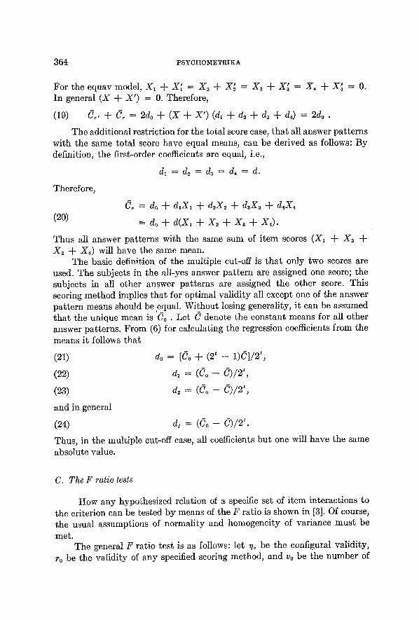
F o r t h e e q u a v model, X 1 -~ X l f ~--- X 2 "4- X~ = X 3 "~-- X~ = X 4 + X41 = 0.

In general (X + X') = 0. Therefore,

(19) C~, -4- C~ = 2do A- (X -4- X') (d, -4- d2 A- da -4- d4) = 2do.

The additional restriction for the total score case, tha t all answer patterns with the same total score have equal means, can be derived as follows: By definition, the first-order coefficients are equal, i.e.,

Therefore,

d~ = d ~ = d ~ = d ~ = d .

(21)

(22)

(23)

and in general

(24 )

C, = do -t- dlX1 -t- d2X~ A- d3Xa -4- d4X~

(20) = do -4- d(X, -f- X~ "4- X3 "F X4).

Thus all answer patterns with the same sum of i tem scores (X~ A- X~ + X3 -4- X4) will have the same mean.

The basic definition of the multiple cut-off is tha t only two scores are used. The subjects in the all-yes answer pattern are assigned one score; the subjects in all other answer patterns are assigned the other score. This scoring method implies tha t for optimal validity all except one of the answer pattern means should be equal. Without losing generality, i t can be assumed tha t the unique mean is Co • Let C denote the constant means for all other answer patterns. From (6) for calculating the regression coefficients from the means it follows tha t

do = [Co + (2t - 1)C]/2',

dl = (Co -

dz = (Co -- C)/2 ' ,

di = (Co - C)/2 t.

Thus, in the multiple cut-off case, all coefficients but one will have the same absolute value.

C. The F ratio tests

How any hypothesized relation of a specific set of i tem interactions to the criterion can be tested by means of the F ratio is shown in [3]. Of course, the usual assumptions of normality and homogeneity of variance must be

met. The general F ratio test is as follows: let 7o be the eonfigural validity,

r0 be the validity of any specified scoring method, and vo be the number of

H . G. OSBURN AND ARDIE L U B I N 365

sample statistics that must be calculated. Then

(25) F = \ 1 - v~,/\2 t - Vo]"

An even more general formula is given in ([3], equation 34).

Worked Example

In order to illustrate the method an example was constructed. Five hundred scores were drawn from a table of normal random deviates. These scores were then transformed so that the universe mean was 5 and the uni- verse standard deviation was 10. The frequencies for each answer pattern were calculated by fixing the p values of the four i tems at pl = .3, P2 = .4 p3 = .5, P4 = .6 and assuming all i tems to be statistically independent. The 500 scores were assigned at random to the sixteen answer patterns according to predetermined frequencies.

To the artificial data described above, a linear systematic component was added. The following arbitrary values were assigned: do = 22, dl = --1, d2 = 5, d3 = - -7 , d4 = 9. Using these values in (14) gave the systematic component that was added to each answer pattern mean. The column in Table 3 labelled C gives the answer pattern mean obtained by these com- putations.

TABLE 3

Basic Data foe Worked Example

Answer Pattern n ~C ZC 2 1 ~(£C)2 Deviance

A 0 YYYY 18 605 22~581 20,334.722 2,246.277 33.611 A l NYYy 42 1,556 61,114 57~646.095 3,467.905 37.048 A 2 YNYY 27 604 17,448 13,511.703 3,936.296 22.370

A 3 yYNY 18 861 42,275 41,184.500 1,090,500 47.833

A 4 YYYN 12 168 3,836 2,352.000 I~484,000 14.000

AI2 NNYY 63 1,725 52,863 47,232.142 5~630.857 27.381

AI3 NYNY 42 1,997 100,023 94,952.595 5,070.405 47.548

AI4 NYYN 28 505 ]I,821 9,108.035 2,712.964 18.036

A23 YNNY 27 947 35~765 33,215.148 2,549,852 35.074

A24 YNYN 18 84 1,972 392.000 1,580.000 4.667

A34 YYNN 12 291 7~813 7~056.750 756.250 24.250

AI23 N~NY 63 2,321 91,363 85,508.587 5~854.413 36.841

A124 NNYN 42 186 5,738 823.714 4,914.288 4.429

AI34 NYNN 28 846 27,548 25,561.285 1,986.714 30.214

A234 YNNN 18 313 6,495 5,442.722 1,052.278 17.389

A1234 NNNN 42 927 24,471 20,460.214 4,010.786 22.071

Total 500 13,936 513,126 388,424.192 124,701.808 27.872

Z~ = 13,935.300 Z~ 2 = 463,601.606 Z~C = 463,603.728

M = 18 XM 2 = 18 ~MC = 861 ZT = II00

^ d c T M

26.423 33.465 2 0 -1.523 36.397 3 0

5.145 23.011 1 0

-6.230 45.745 3 ]

9.541 14.679 l 0

- .121 25.943 2 0

- .007 48.677 4 0

.282 17.611 2 0

• 336 35.291 2 0

.402 4.255 0 0

.369 26.959 2 0

- .217 38.223 3 0

.574 7.157 1 0

- .863 29.891 3 0

-.656 16.505 1 0

• 157 19.437 2 0

33.612 423.216

ZT 2 = 2,890 ~'TC : 36,011

366 PSYOHOMETRIKA

Step 1--Calculation of the configural validity

First, a one-way analysis of variance is computed. The column labelled deviance in Table 3 contains the sum of squared deviations (sum of squares) about each answer pattern mean. The sum of the 16 answer pattern deviances is W, the within group sum of squares. The column labelled ( ~ C)~"/N contains a correction term for each answer pattern. The sum of the 16 cor- rection terms minus the correction for the total equals B, the between group stun of squares.

TABLE 4

Analysis of Variance

Source df Deviance Mean Square

Between Answer ~atterns 15

Within 484

Total 499

2= C .612

76,358.028 5,090.535

48~343,784 99,884

124,701.804

F = 50.964

These figures along with T, the deviance (sum of squares) about the total mean, are given, in the usual analysis of variance form, in Table 4. The formula for the configural validity is

(26) ~ = B / T - 76,358.020 _ .612325. 124,701.804

The test of significance is

( .1 (.612325 (484 (27) F = \ l - - E - ~ j \ ~ _ l ] = \ ~ / \ - - ~ / = 50.964.

Since the .001 confidence level is 2.577, the eonfigural validity is obviously greater than zero. If the F ratio was insignificant, the analysis would be stopped, for then no method of scoring the test would give a better-than- chance prediction of the criterion scores.

Step 2--Calculation o] the polynomial regression coe~cient's

In Table 3, the column labelled d contains all 16 polynomial regression coefficients. Each coefficient was computed by adding together the 16 means (appropriately signed) and dividing by 2'. The sign of each mean is given by ( - 1 ) ", where g is the number of common items in the subscripts of the regression coefficient and the mean.

I-I. G. OSBURN AND ARDIE LUBIN 367

For example,

1 do = ~ [ 0 o + 0 , + 0 ~ + C 3 + C , + 0 1 ~ + 0 1 3 + 0 1 ~ + 0 5 3 + 0 5 4

~- 034 ~- 0123 ~- C124 ~- 0134 -I- 0234 -~ C1234] = 422.762 16 = 26.423,

1 dl = ~[0o-- 0 , + 0 5 + C3 + C , - 0 ,2 - 0 ,3 - 01 ,+023+ 024

~- 034 -- 0123 -- 0124 -- 01"3, -~- 0234 -- 01234] = - - 2 4 . 3 7 4 16 -- --1.523,

1 d,5 = ~ [0° - ¢1 - 05 + 03 + 04 + 015 - 013 - 01, - 02, - 0~4

+ C34 + ¢153 + ¢154 - 0,34 - 0534 + 01~,4] -1 .930

16 .121,

and so on. These coefficients can be scanned in order to see which scoring method

seems to give an optimal prediction of the criterion with the fewest parameters. For example, if, in the population, the relation between the items and the criterion were exactly linear, the only nonzero coefficients would be do, d l , d5, d3, and d4. In any actual sample, the other nonlinear coefficients would be small but not exactly zero. So one can simply look at the five linear co- efficients to see if their absolute values are larger than any of the other coefficients. Another such test is to check the frequency of negative values among the eleven non linear coefficients. In the linear case, the true probability of a negative value is 1/2. If these crude combinatorial tests do not contradict the hypothesis of linearity we proceed to the next possibili ty--that the total score will give maximum validity.

The total score will give maximum validity in the population when all the conditions for linearity are met and in addition, [ dl [ = [ d5 1 = I d3 ] = ] d4 I; i.e., the absolute values of the first-order coefficients are equal. Again, a crude check of this can be made in the sample by seeing if there is wide variation among the absolute values of the first-order coefficients.

In Table 3 it can be seen tha t the linear coefficients (do , d, , d2, d3 , and d4) meet the first condition; their absolute values are larger than those of the nonlinear coefficients. Also the second condition is met; the ratio of negative nonlinear coefficients was 4/11, which is not significantly different from the expected value of 1/2. Therefore, the hypothesis of linearity is not contradicted.

Next the first-order coefficients were examined to see if the total score was likely to have maximum validity. If so, the first-order coefficients (dl ,

368 PSYCHOMETRIKK

d2 , da , and d4) would be approximately equal. But d4 was more than six times the absolute value of d~ . So it is unlikely tha t total score would have maximum validity.

As mentioned earlier the above crude tests can be used if the research worker has no definite hypothesis about the optimal scoring method. However, to demonstrate conclusively tha t linear scoring is sufficient for optimal brediction it is necessary to show that the multiple correlation, Ro.~,2.8.4 , does not differ significantly from the configural validity ~ . To demonstrate conclusively that linear scoring is preferable to the total score and the multiple cut-off score, it has to be shown that the total score validity and the multiple cut-off validity are significantly less than the configural validity.

,Step 3--Calculation o] the multiple correlation

In Step 2, the linear hypothesis passed the first crude tests. To compute the linear multiple correlation R~.~.2,3.4 first C~ , the predicted criterion score for the rth answer pattern, was calculated. (This may not be the most convenient method, but it does show any large deviations from the linear hypothesis. For a perfect linear fit, C, = C~, .) To obtain ~ it was first neces- sary to compute the linear regression coefficients; i.e., w0 , w~ , w2 , w3 , w, from (18).

The matrices (K~nK~), (K;nK~) -~ and (K~nC) are presented in Table 5. The regression coefficients are in the column w. Then C was obtained by applying the equation ¢ = K,w. The predicted criterion means are presented in the ~ column of Table 3. Ro,1.2,3,4 is equal to ro~ , the zero-order correlation

TABLE 5

Computation o f L i n e a r R e g r e s s i o n C o e f f i c i e n t s

x 0 x I x 2 x3 x 4

X 0 500 -200 -I00 0 i00

X 1 -200 5C0 40 0 -40

X 2 -I00 40 500 0 -20

x 3 o o o 500 o

x 4 lOO -4o -2o o 500

Sum 300 300 420 800 540

X 0 X 1 X2 X 3 X 4

X 2.548 .952 .417 0 - ,417 13~936 26.451 0

X 1 .952 2.381 0 0 0 -6,190 -1.466

K 2 .4 [7 0 2.083 0 0 -278 D.227

X 0 0 0 2.000 0 -3~070 -6.140 3

X 4 - .417 0 0 ~ 0 2.083 7~296 9.393

3.500 3.333 2.500 2.000 1.666 11~694 33.465

between C and ~. This was computed by the well known formula

= _ E •

H . G. O S B U R N A N D A R D I E L U B I N 369

Column ~ C in Table 3 contains the sums of the criterion scores for each answer pattern. To obtain ~ C C, each Cr was multiplied by the ~ C for the rth answer pattern, and the result was summed over all patterns.

Similarly, 2t 2 t

E O ~ = E n r O ~ = E O C and E 0 = E n , O , = E C -

Substituting in (28) from the data in Table 3,

2 [500(463,603.728) -- 13,936(13,935.300)] 2 r~ = [500(513,126) -- (13,936)2][500(463,601.606) -- (13,935.300) 2] -- .603.

Step 4--Comparison of the multiple correlation with the configural validity

Applying (25),

( . 6 1 2 - . 603~(500- ~6) F = \- .~-~8 ~ ] \ ~ _ - = 1.021.

Since, for 11 and 484 d.f., the .05 level is 1.750, the F test indicates that the multiple correlation does not differ significantly from the configural validity; i.e., the multiple regression scoring method yields optimal validity.

Step 5--Calculation of the total score validity

In order to rule out conclusively the total score hypothesis, the zero- order correlation r, was computed between the total score and the criterion. In general, the total score, T, is equal to the number of yes responses for all items with positive first-order coefficients plus the number of no responses for all items with negative first-order coefficients. The column labelled T in Table 3 gives the total score for each answer pattern. The usual formula for the squared correlation was used.

(29) r~ = (N E CT - ~ C E T) 2 [(N ~ C 2 - (~-~ C)2][N ~ T 2 - (~--~ T) 2]

Using the data from Table 3,

2 [500(36,011) -- ( 13,936) (l , 100) ]2 r, = [500(513,126) -- (13,936)2][500(2,890) ' - (1,100)21 = .489.

Step 6--Comparison o] the total score validity with the configurat validity

Applying (25),

F = \ . ~ / \ - ~ _ = 10.960.

Since, for 14 and 484 d.f., the .05 level is 1.690, the F test indicates that

370 PSYCHOMETRIKA

the total score validity is significantly less than the configural validity, i.e., the total score does not yield optimal validity.

Step 7--Calculation ol the multiple cut-off validity

In order to rule out conclusively the multiple cut-off hypothesis, the zero-order correlation, r~o , was computed between the multiple cut-off score and the criterion. Multiple cut-off scoring demands that a score of one be assigned to the answer pattern with the highest (or lowest) mean and that a score of zero be assigned to all other answer patterns'. Column M in Table 3 gives the multiple cut-off score for each answer pattern. Substituting figures from Table 3 into the formula for squared correlation;

r 2 = .... [500(861) - 18(13,936)] 2 mo [500(513,126) -- (13,936)2][500(18) - (18) 2] - .060.

Step 8--Comparison o/the multiple cut-off validity with the configural validity

Applying (25),

( . 6 1 2 - .060~(500- 16~ F = \- .3-88- / \ 1 6 - 2 '/ = 49.185.

Since, for 14 and 484 d.f., the .05 confidence level is 1.690, the F test shows that the multiple cut-off validity is significantly less than the configural validity.

Discussion

I t has been shown how the concept of the configural scale can be used to give an exact statistical test of whether a selected scoring technique has optimal validity. Worked examples have been given for three well known test scoring methods: multiple regression, multiple cut-off, and total score. In general, the principal advantage of configural analysis is that all of the information concerning the subject's test behavior is utilized.

On the other hand, the principal disadvantages of configural analysis lie in the very fact that all the information is conserved; i.e., all possible answer patterns are considered. In a t-item test the formula for the configural validity involves 2 ~ parameters; i.e., 2 * answer pattern averages. I t is im- mediately obvious that this technique is only appropriate for situations where the number of items is very small compared to the number of subjects-- N must be much greater than 2'. For example, even when the number of items is as small as 10, 2' will be 1024.

Use of the equav coefficients for scanning purposes introduces another difficulty. The F ratio test no longer gives the exact confidence level; it is simply a decision function. The procedure of selecting the test scoring method which is most likely to yield optimal validity alters the significance level of

H . G. OSBITRN AND ARDIE LUBIN 371

the F test (cf. [2], p. 199 ft.). As a way of deciding among several possible test scoring methods, the scanning technique is certainly a reasonable pro- cedure. However, it is advisable, after selecting a test scoring method on one sample, to cross-validate it on another sample.

Configural analysis is most suitable in situations where testing time is short and the number of subjects is large. For example, take the case of neuropsychiatric screening in the armed forces where often only a few minutes of testing time is available, and a very large number of subjects must be screened. Here, items should be constructed in such a way that all 2' regression coefficients are significant. This will give maximum discrimination. However, in actual practice some of the regression coefficients will probably be non- significant. If this occurs, a value of zero should be given to all nonsignificant coefficients. The use of any other values will lower the validity of the test.

REFERENCES [t] Horst, P. Pattern analysis and configurM scoring. J. clin. Psychol., 1954, 10, 3-11. [2] Kendall, M. G. The advanced theory of statistics. Vol. II. London: Griffin, 1948. [3] Lubin, A. and Osburn, H. G. A theory of pattern analysis for the prediction of a

quantitative criterion. Psychometrika, 1957, 22, 63-73.

Manuscript received 12/7/56

Revised manuscript received 4/18/57