the two-frequency, two-time coherence function for the fluctuating ionosphere: wideband pulse...

Pergamon Journal ofArmo.pheric and Solar-Terreswiai Physics, Vol. 59. No. 14, pp. 1X43-1854, 1997

rci 1997 Elsevier Science Ltd

PII: S1364-6826(97)00012-6 All rights reserved. Prmted in Great Bntarn

13646826/97$17.00+0.00

The two-frequency, two-time coherence function for the fluctuating ionosphere: wideband pulse propagation

Vadim E. Gherm,’ Nikolay N. Zernov’ and Bengt Lundborg’,*

‘Institute of Radiophysics, University of St. Petersburg, Ulyanovskaya 1, Petrodvorets, 198904, St. Petersburg, Russia and *Swedish Institute of Space Physics, Uppsala Division, S-755 91,

Uppsala, Sweden (e-mail: [email protected])

(Received 8 July 1996; revised 10 January 1997; accepted 13 January 1997)

Abstract-This article presents a numerical investigation of the two-frequency, two-time coherence function for HF wave propagation in the fluctuating ionosphere. Earlier published results of numerical calculations, with an empirical plane-stratified background ionosphere and a power-law spectrum of the electron density fluctuations, show that the coherence function in general has a rather complicated behaviour and that it does not fall off quickly with increasing difference frequency. Under these circumstances, the case of wideband pulses requires particular considerations which are presented in this article. The shape of a wideband pulse is generally represented by two items, namely the contributions from the fluctuational and coherent components of the field that has passed through the fluctuating ionosphere. 0 1997 Elsevier Science Ltd

1. INTRODUCTION

With this article we continue our study of the influence of ionospheric electron density fluctuations on pulse propagation through the ionosphere. The investigation was started in the article by Zernov and Lund- borg (199.5) where the main analytical relations were derived on the basis of Rytov’s approximation generalized in Zernov (1980) to the case of inhomo- geneous background media with local embedded inhomogeneities. It was continued in Gherm er al. (1997) where the previously obtained analytical results were employed in a detailed numerical analysis of the two-frequency coherence function. Our numerical results were then used in a quantitative description of the effects of electron density fluctuations on narrowband pulse propagation through the ionosphere. Concerning the problem of wideband pulse propagation, the investigations in Gherm et al. (1997) dem- onstrated the necessity of further development for its treatment. This is the subject of the present article.

2. TIME COHERENCE OF A NONSTATIONARY FIELD

We shall no;N consider the two-time coherence function of a pulsed signal E(r,t) which reaches the point

*Now at: Defence Research Establishment, P.O. Box 1165, S581 Linkoping, Sweden.

of observation r after passing through the fluctuating ionosphere. It is given by the following expression:

f&,t,,t,) = <E(r,tJE*(r,tJ). (1)

As in Zernov and Lundborg (1995), we describe a harmonic component E,(r,t) of the signal in the isotropic approximation by a scalar equation of the form;

V2E,,+k2[~,(z,o)+~(r,w,t)lE,, = 6(r). (2)

Here E,,(z,w) is the model of the undisturbed plane- stratified background ionosphere, whereas a(r,W,t) represents the local random inhomogeneities of the ionosphere. Time t in (2) stands for a possible slow time dependence of the fluctuations in the quasi- stationary approximation. The condition of validity of this approximation for a dispersive plasma is given by the inequality

TV>> 1, (3)

where T is a characteristic time scale of the nonstationary and r is an effective collision frequency of the plasma electrons so that v-’ gives the relaxation time scale of the ionospheric plasma.

The undisturbed field E:)(r) is described in the geometrical optics approximation and is given by equations (5-11) in the article by Zernov and Lundborg (1995) or, in the 3D case, by equations (3-9) in Gherm et al. (1997). The influence of the local inhomo-

1843

1844 V. E. Gherm et al.

geneities in the ionosphere is accounted for by means of a complex phase $(r,w,t) so that the disturbed field E,(r,t) is of the form:

&(r,t) = -C’(r) exp [W,w)l. (4)

We shall construct the two-time coherence function of a pulse signal which has propagated through the fluctuating ionosphere in the form of a double integral in the frequency domain as follows.

x Ur,wrw,tl,f2) exp (i{k4dr,w,441

-Wh.d~dw4~2)1J - ibIt, -Wd. (5)

Here k, = q/c, k, = WJC and c is the velocity of light in a vacuum;Qr,w,cc(w)] and $,[r,w,cc(w)] are the amplitude and phase of the undisturbed field E$” in the plane-stratified ionosphere written in the geometrical optics approximation. The argument R(W) is written out to indicate the implicit w-dependence via the launching direction CC. The function r(r,w,,w2,t,,tZ) is the two-frequency, two-time coherence function at the point r with the slow time-dependencies t,, tz in the sense discussed previously. This is essentially the same function as was constructed in Zernov and Lundborg (1995) by making use of the first and second approximations of the complex phase $(r,w,t). It is given, with the time-dependence suppressed, by the expressions (32-34) in that article.

Here we shall use the following representation of the coherence function:

I(rrwliw~,fl,fZ) = 12(rrWI,WZ,rlrt2), (6)

which is convenient for further exploitation. After decomposition of the different orders of complex phases into real and imaginary parts,

ti, = xi+& tit = x2+& (7)

we can express the coherence function (6) as follows:

I,(r,w,,w,,t,,r,) = V,(r,w,,t,)l/:(r,w,,t,)

x exp [b(r,w,,wJ,,t,)+ iq(r,w,,w,,r,JJl (8)

where,

V&.w,t) = exp [(~~(w,r)) + i<&(w,O)l

+ f <XXWJ)> + ~(Xl(w,fMw,o) - ; <~Xw))

W,w,m,,t,,b) = <xdwJJxl(wd2)> + (S,(w,,t,)S,(w*,t,)), (9)

- (X,(w,,tl)s,(W*,t,)>.

Subscript 2 on I1 and V, means that these quantities are calculated with the first and second approximations of the complex phase. In contrast, b and q only require the first approximation. For convenience, the argument r was omitted in the right-hand sides of

(9). If stationarity is assumed for the random process

of ionospheric fluctuations, we may immediately conclude that P’*(r,w,t) no longer depends on t, and that b and q in (9) depend on the difference t, -t,. Then the two-frequency, two-time coherence function is actually of the form

12(r,W,,W2,tl,f2) = V,(r,wr) V: (r,wJ

x cxp Mr,w+M+ iq(rr~dM)l (10)

with t = t, - t2. The quantities Vz, b and q are expressed through the moments of the complex phases rj, and tiz in (9) and are the same as in equation (20) in the companion article (Gherm et al., 1997) with the time-dependence recovered wherever necessary.

The function (10) is the fundamental quantity when considering the influence of ionospheric electron density fluctuations on pulse propagation. In the next section, we discuss the properties of this function in some detail.

3. TWO-FREQUENCY, TWO-TIME COHERENCE

FUNCTION

It is obvious that the mean energy of a pulse which has propagated through the fluctuating ionosphere is a particular case of the time-coherence function (5) with coinciding time arguments:

WE@,0 = I.&N. (11)

When we wish to calculate the mean energy it is hence clear that we need the two-frequency coherence function with zero time argument, rz(r,w,,w,,O), which can be expressed as follows:

I&w,,@ = V,(r,w)K+ (r,mJ

x exp [b(r,w,,wz,O)+ idr,w,,wdU. (12)

This function was thoroughly investigated in Gherm et al. (1997) in numerical calculations of the moments in relations (8) and (9), expressing the electron density fluctuations in terms of the inverse power- law spatial spectrum model according to (28) in that

HF pulse propagation through a fluctuating ionosphere: wideband 1845

article. It was studied as a function of the centre and difference frequencies

n=;(C0~im2); 6=w,-w* (13)

in the HF band for different parameter values of the ionospheric fluctuations. The results of the calculations were plotted as Figs l-5 in Gherm et al. (1997).

The present function (10) is more general than (19) in Gherm et al. (1997) through its nonzero time argument. For a fixed point of observation it is a function of three variables and different projections are needed to illustrate its behaviour. For further consideration and, in particular, for the calculation of wideband pulse propagation, it is necessary to extract in explicit form the behaviour of the function r2 on the difference frequency variable at infinity. To this end we shall make use of a well known relationship (Rytov et al., 1978) between the coherence function and the correlation function, which we denote as Y’,. It is as follows:

The last equation together with (10) immediately gives for the two-frequency, two-time correlation function the expression

Y’,(r,Q,6,t) = Vz r,R+ i6 ( 1

x Vf r,R- 16 F(r,QY,t), (15) ( 1

with

F(r,C&Y,t) = exp[b(r,CQ,t)+iq(r,Qd,t)]-1.

(16)

As mentioned already, the quantities IY2 and Y’, are functions of three variables in the frequency-time domain for a fixed point of observation r. Different projections of these functions are needed for considering different physical problems. One of the projections, namely rz(r,Q,6,0), investigated thoroughly in Gherm et al. (1997), is necessary for pulse propagation study, which we shall address in the next section of the article. Other projections are involved in the interpretation of different effects of multi-frequency ionospheric sounding. We intend to pay special atten- tion to this complicated problem in a separate article.

One of the projections is the function r,(r,R,G,t) in the domain (6,t) for fixed r and R. Some con-

siderations of this projection were given in Fridman et al. (1995). Strictly speaking, they studied the function b(r,!&?,t) from equation (16) in the domain (6,t) for a Gaussian law of the spatial spectrum of the ionospheric electron density fluctuations, and they did not consider any imaginary part q(r,R,&t). In the companion article (Gherm et al., 1997) we have already discussed the correspondence between our method of calculating the coherence function and that used by Fridman et al. (1995). Below we give the treatment of the coherence and correlation functions in the scope of our approach.

For calculation of the quantity b(r,Q,b,t)+ iq(r,Qh,t) in the time domain we shall use the representation of this sum derived in Gherm et al. (1997) (equation (20)) with the temporal variables recovered as follows:

where t = t, - t2. We will adopt the model of ‘frozen- drift’ to account for the motion of the ionospheric random irregularities. In this case the time-dependent spatial spectrum of the correlation function of fluctuations assumes the form:

B,(K, t) = 1 dw exp ( - iox)B,(zc)6(rc * v - co)

= B,(ic)exp(-ii~*vt), (18)

where v is the drift velocity vector. Then, according to Gherm et a/. (1997) and taking into account (17), ( 1 S), the function b + iq has the form

k,k, .‘Q b(r,QQ)+ iq(rMJ) = 4

s

ds o [E0(S,)E0(S2)],i2

. Jj dK, d@(O,K,,K,) exp {&IA(s) - Ml - iKPJj

(19)

Here k, and k, are the vacuum wave numbers of the two frequencies; the integration over s is performed along the ray for the centre frequency R; the perpendicular through this point crosses the neigh- bouring rays for w, and w2 at the points with coordinates s, and sz, respectively; A(s) is the distance between the points s, and s,; v, and v, are the projections of the drift speed on the directions normal to the ray, it is in the plane of propagation and z is perpendicular to this plane. In the limiting case of the

geometrical optics approximation, i.e. when diffraction can be neglected, expression (19) actually becomes of the same form as equation (14) in Fridman et a/. (1995). This limit is formally reached in the case of zero values of the quantities D,, D, in equation (19). Then it yields q = 0 and the double integral over wave numbers K,, K, in the representation for b produces the spatial correlation function of the ionospheric electron density fluctuations. In our case of an isotropic inverse power-law spectrum according to (28) in Gherm et al. (1997), the spatial-temporal correlation function is as follows:

where K, is the modified Bessel function of the second kind of order v.

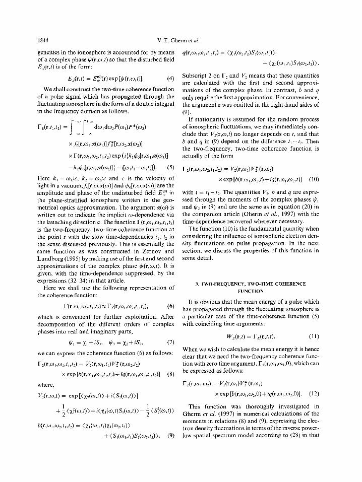
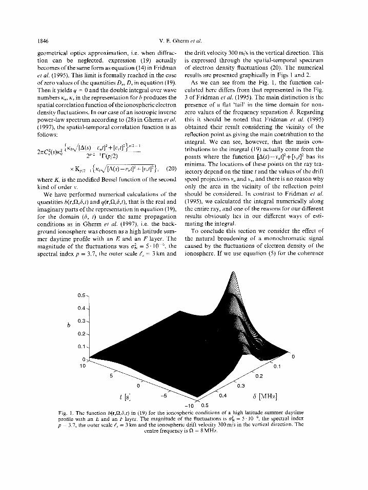
We have performed numerical calculations of the quantities b(r,R,G,t) and q(r,R,S,t), that is the real and imaginary parts of the representation in equation (19) for the domain (6, t) under the same propagation conditions as in Gherm et al. (1997) i.e. the background ionosphere was chosen as a high latitude summer daytime profile with an E and an F layer. The magnitude of the fluctuations was 0; = 5. 10m6, the spectral index p = 3.7, the outer scale 8,. = 3 km and


the drift velocity 300 m/s in the vertical direction. This is expressed through the spatial-temporal spectrum of electron density fluctuations (20). The numerical results are presented graphically in Figs 1 and 2.

As we can see from the Fig. 1, the function calculated here differs from that represented in the Fig. 3 of Fridman et a/. (1995). The main distinction is the presence of a flat ‘tail’ in the time domain for nonzero values of the frequency separation 6. Regarding this it should be noted that Fridman et al. (1995) obtained their result considering the vicinity of the reflection point as giving the main contribution to the integral. We can see, however, that the main contributions to the integral (19) actually come from the points where the function [A(S)-v~]*+[v,t]* has its minima. The locations of these points on the ray tra- jectory depend on the time t and the values of the drift speed projections v, and v,, and there is no reason why only the area in the vicinity of the reflection point should be considered. In contrast to Fridman et al. (1995) we calculated the integral numerically along the entire ray, and one of the reasons for our different results obviously lies in our different ways of esti- mating the integral.

To conclude this section we consider the effect of the natural broadening of a monochromatic signal caused by the fluctuations of electron density of the ionosphere. If we use equation (5) for the coherence

b

-10 0.5 Fig. 1. The function b(r,Q,d,t) in (19) for the ionospheric conditions of a high latitude summer daytime profile with an E and an F layer. The magnitude of the fluctuations is g’, = 5. 10e6, the spectral index p = 3.7, the outer scale /, = 3 km and the ionospheric drift velocity 300m/s in the vertical direction. The

centre frequency is R = 8 MHz.


0.01

0

q -0.01

-0.02

-0.03 10

Fig. 2. The quantity q(r,R,i?,t) in (19) for the same situation as in Fig. 1

function IE with the spectrum P(w) expressed by Dirac’s function

P(w) = Hb(w-W”), (21)

where w0 is the frequency of the sounding field, we immediately obtain the following result:

f&J) = I~l”lfo[r~~0~~(~0)l12

x r2(r,w,,o,,t) exp (- iw,t). (22)

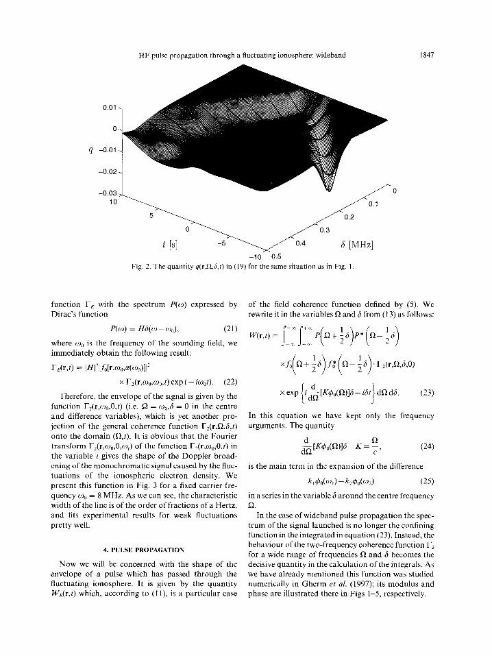
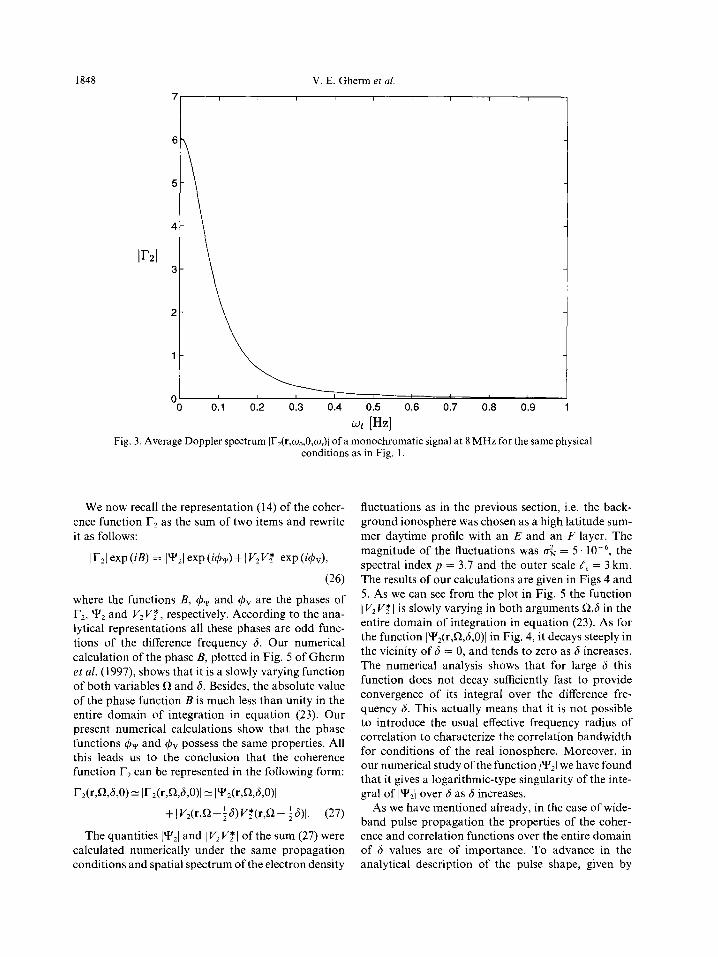
Therefore, the envelope of the signal is given by the function r,(r,w,,O,t) (i.e. 52 = w,,6 = 0 in the centre and difference variables), which is yet another projection of the general coherence function r,(r,R,G,t) onto the domain (C&t). It is obvious that the Fourier transform r2(rrW0,0,q) of the function rz(r,w,,O,t) in the variable t gives the shape of the Doppler broadening of the monochromatic signal caused by the fluctuations of the ionospheric electron density. We present this function in Fig. 3 for a fixed carrier frequency w0 = 8 MHz. As we can see, the characteristic width of the line is of the order of fractions of a Hertz, and fits experimental results for weak fluctuations pretty well.

4. PULSE PROPAGATION

Now we will be concerned with the shape of the envelope of a pulse which has passed through the fluctuating ionosphere. It is given by the quantity IVE(r,t) which, according to (1 l), is a particular case

of the field coherence function defined by (5). We rewrite it in the variables R and 6 from (13) as follows:

,,.t)=S_:S:‘P~+fn)P*(I)-Ih)

xexp i$[Ky’,,(B)]6-iht (23)

In this equation we have kept only the frequency arguments. The quantity

is the main term in the expansion of the difference

k,4&(w,)-k*~,(%) (25)

in a series in the variable 6 around the centre frequency n.

In the case of wideband pulse propagation the spectrum of the signal launched is no longer the confining function in the integrated in equation (23). Instead, the behaviour of the two-frequency coherence function fZ for a wide range of frequencies s2 and 6 becomes the decisive quantity in the calculation of the integrals. As we have already mentioned this function was studied numerically in Gherm et al. (1997); its modulus and phase are illustrated there in Figs l-5, respectively.

1848 V. E. Ghenn et al.

0 0.1 0.2 0.3 0.4 0.5 0.6 0.7 0.8 0.9 1

w [Hz] Fig. 3. Average Doppler spectrum 11-2(r,00,0,w,)J of a monochromatic signal at 8 MHz for the same physical

conditions as in Fig. 1.

We now recall the representation (14) of the coherence function r2 as the sum of two items and rewrite it as follows:

IF21 exp (i-B) = IYJ exp (i&) + I V2v?* I exp (~~v)~

(26) where the functions B, c#+ and & are the phases of r2, YZ and V,V:, respectively. According to the analytical representations all these phases are odd functions of the difference frequency 6. Our numerical calculation of the phase B, plotted in Fig. 5 of Gherm et al. (1997), shows that it is a slowly varying function of both variables fi and 6. Besides, the absolute value of the phase function B is much less than unity in the entire domain of integration in equation (23). Our present numerical calculations show that the phase functions & and & possess the same properties. All this leads us to the conclusion that the coherence function T2 can be represented in the following form:

r,(r,fi,a,o) = lr,(r,0,6,0)1= iwmu9

+IV2(r,R+~6)Vt(r,C2- f6)l. (27)

The quantities lY’21 and I V, Vf I of the sum (27) were calculated numerically under the same propagation conditions and spatial spectrum of the electron density

fluctuations as in the previous section, i.e. the background ionosphere was chosen as a high latitude summer daytime profile with an E and an F layer. The magnitude of the fluctuations was cr’, = 5. 10e6, the spectral index p = 3.7 and the outer scale !, = 3 km. The results of our calculations are given in Figs 4 and 5. As we can see from the plot in Fig. 5 the function ) Vz VF I is slowly varying in both arguments R,6 in the entire domain of integration in equation (23). As for the function lY’2(r,R,6,0)j in Fig. 4, it decays steeply in the vicinity of 6 = 0, and tends to zero as 6 increases. The numerical analysis shows that for large 6 this function does not decay sufficiently fast to provide convergence of its integral over the difference frequency b. This actually means that it is not possible to introduce the usual effective frequency radius of correlation to characterize the correlation bandwidth for conditions of the real ionosphere. Moreover, in our numerical study of the function )YS) we have found that it gives a logarithmic-type singularity of the integral of lYZ/ over 6 as 6 increases.

As we have mentioned already, in the case of wideband pulse propagation the properties of the coherence and correlation functions over the entire domain of 6 values are of importance. To advance in the analytical description of the pulse shape, given by


8.5

Fig. 4. The modulus of the correlation function Y,(r,QJ,O) in (27) for the same situation as in (Gherm ef al., 1997) i.e. a high latitude summer daytime profile with an E and an F layer and the fluctuations

described by e’, = 5. 10m6,p = 3.7, and d, = 3 km.

0.5

0.4 *

Iv2vzl 0.3

0.2

0.1 /-8.5

Fig. 5. The modulus of the quantity V*(r,Q +i 6) V:(r,Q - i 6) in (27) for the same situation as in Fig. 4.

equation (23) we therefore adopt a particular model already studied its behaviour in the vicinity of 6 = 0 of the correlation function )Y’,l in (27) of the following and found that it has a narrow peak of Gaussian type, form: which is of importance in the case of narrowband

IY2(r,GW)I = a*(r,Q)[l +Y(~,WT’. (28) pulse propagation (Gherm et al., 1997). Now we are mterested in the nronerties of the correlation function

Here cr*(r,R) is the variance of the field fluctuations over a wider in&al, instead, and the model (28) at the point r as function of the frequency 52. This was chosen to provide the same type of logarithmic model does not reflect the behaviour of the exact cor- divergence of the integral of JYJ over 6 as the numeri- relation function for small 6. However, we have tally calculated integral demonstrates. The numerical


value of y(r,Q) is a coefficient determined from the logarithmic function, calculated for fixed r,Q and d(r,R). This coefficient has the dimension of time and characterizes the scale of decay of the function ]Y’2] in equation (28). Hence, we can consider the quantity

Y _I as a generalized characteristic of the correlation bandwidth for the case of a slowly decaying correlation function.

The relationships (27), (28) yield for the mean energy of the monochromatic component of the field W,(r,Q), normalized to the energy of the undisturbed field, the following representation:

q,,(r,a) = f,(r,GO,O) = o*(r,fi) + I V2(r,W. (29)

In contrast:

expressed as the sum of two terms. These two terms represent the contributions of the fluctuational and coherent components, respectively, to the shape of the full field of a pulsed signal. Obviously, the factor f. in both terms represents the frequency dependent amplitude of the ray field in the background ionosphere and can be treated as a very slowly varying function, as its characteristic frequency scale is of the order of the plasma frequency of the ionospheric F-layer. Then we can always write;

.6(n+ ;gfC(n- ;+fo~w (35)

f&$X&O) = exp [hdr,~K 4.1. Coherent$eld

Bdr,f4 = 2(x&S)) +2(xXr,Q)), (30)

where the quantity f10 is the same as (39a) in Zernov and Lundborg (1995). The two items in the sum (29) describe the decomposition of the mean energy of the monochromatic field into the fluctuational and coherent components.

Finally, putting together (23) (27) and (28), we obtain the following expression for the mean energy of a wideband pulse which has propagated through the fluctuating ionosphere:

We start investigating the sum (31) by analyzing the second term, which represents the coherent part of the mean energy of the pulse. As we have already mentioned, the function 1 V, Vf I is slowly varying in the variables Q6. We can see from the plot in Fig. 5 that it is almost constant as a function of 6, and that it is slowly dependent on the centre frequency R, so that we can also write to zero-order approximation

1 Y,(R+:6)l’f(R--:n)l=lc:(n)i, (36)

W(r,t) = W’)(r,t)+ W(*)(r,t), (31) while evaluating the integral over 6 in equation (33). To proceed with calculating this integral, we assume the spectrum P of the pulse launched to be wider than the bandwidth of the background ionospheric channel. This means that to the zero-order approximation the following relationship can be written as well: x o’(r,R)[ 1 + ylS\]-’ exp { -it’d} da d6,

(32)

x exp { - it’6) dR d6,

where t’ is given by the relationship;

t’ = t - $ [K~,(R)].

As we can see, the envelope of the pulse energy is

(33)

(34)

,(,,+ ~~)P.(,- +w2v. (37)

Then after integration over 6 equation (33) yields:

W@)(r,t) = 27~ s

+a, l~~~~l’lfo~~~121~~~~,~~l’~~~‘~~~l dQ. -II (38)

Here s[t’] is the Dirac’s function. Choosing t’ as the new variable of integration and writing

dt’ (39)


finally we find

with o0 = w,(t), defined by the relationship

(41)

W’)(r,t) = y-’ s +m IP(s2)l'lf~(n)l'a'(r,~)G ,Z

(44)

where

G(y) = -?[cos(s)Ci(G) + sin(JSi(t)],

This means that, in this approximation, the coherent part of the field at any particular instant is given by the power of the frequency component of the initial pulse that arrives through the background ionosphere at that instant, multiplied by a propagation factor.

It can be shown in a more detailed treatment, where the full asymptotic series is constructed, that for the expression (40) to be valid the pulse length T,, must fulfil

(42)

This condition simply says that the width of the spectrum of the pulse launched must exceed the bandwidth of the undisturbed ionospheric channel.

4.2. FluctuationalJield

Now we deal with the first term in the sum (31) which is given by equation (32) and describes the fluctuational part of the pulse mean energy. In the integrand of (32) there occur three functions with characteristic frequency scales, which are the width T;’ of the spectrum of the radiated pulse, the bandwidth

of the background channel (see Lundborg, 1990) and the generalized correlation width y-l, introduced above. To obtain some analytical results for the integrals in equation (32) we assume now the width of the pulse spectrum to be greater than both the other two scales, i.e. that the inequality (42) as well as

T,<Y (43)

are fulfilled, so that we can again use the approximation (37). Then the integration over the variable 6 in equation (32) can be performed explicitly. The result of this integration is expressed through the sine and cosine integrals as follows:

(45)

and the function t’(R) was defined in (34). The function G(t’/y) has an integrable singularity at the point t’ = 0 and the product y-‘G(t’ly) gives rise to Dirac’s d-function as y+O.

In order to give a correct evaluation of the integral in equation (44), we rewrite the functions in its integrand with dimensionless arguments as follows:

+ = W(“(r,t) = y-’ 1’ IWo~)121hhd412

x a*(q,,R)G y dR. (46) (’ >

Here T;’ is the width of the pulse spectrum, which was introduced already. As for the quantities rO,, t,,2, these are very small values which characterize a very slow frequency dependence in the functions f. and c?. We already mentioned that r,’ is of the order of the plasma frequency of the F-layer. The quantity r,’ is of the same order. Written in this way all the factors in the integrand of (46) vary as functions of their arguments on a scale which is of the order of unity.

Next we introduce a new dimensionless variable x of integration in equation (46) as follows:

t’(Q) -=,y Y ’

so that,

(47)

(48)

The second item in the last sum was omitted, because r(Q) is almost constant as a function of R. Then in the new variable x:

W(‘)(r,t) = s

+- IP(To~(x))l’lfo(~o,~(x))12 -cc

(49)

1852 V. E. Ghenn et al.

Here the dependence Q = Q(x) is given implicitly through equation (47) (34). The function G(x) defined by expressions (45) (47) has an integrable singularity. Its characteristic scale in the dimensionless universal variable x is unity and it is normalized so that

s

+3j G(x) dx = 27r. (50)

--II

The functions ]jb]‘,cr2 and [dt’/dn]-’ under the integral in equation (49) are obviously slowly varying over the range of the characteristic scale of the function G(x), which is x = 1. To understand whether the function ]P(T,R(x))]~ is a slowly varying function on the same scale or not, we must determine the increment of its dimensionless argument as the increment of the variable x is equal to unity, i.e. we must determine the quantity

A[ToR(x)l = T,gAxl,,_,. (51)

With relationships (34) (48) taken into account the last equation yields:

A[T&(x)l = YTll

2 [@II(Q)1

(52)

Hence it is clear that the function ]P]’ is not slowly varying in the sense needed if A > 1. In this case equation (49) gives the ultimate representation of the fluctuational part of the mean energy of a pulse. It is proportional to

s + 3c ]P( TOR(x))l*G(x) dx --n;

and must be calculated numerically for given models of the pulse spectrum.

In contrast, the function ]P]* does not vary essentially over the range 1x1 I 1 if A < 1, that is if

To< [v(w)l-‘{ &&(~)] 1. (53)

When inequality (53) holds, the function ]P]’ can be considered slowly varying over the variable x, can hence be taken out of the integration in (49) and given its value at the point x = 0 with the time dependence w0 = we(t) appearing implicitly through equation (41).

Then, finally, we obtain the result of the integration in (49) or (44) as follows:

W(‘)(r,t) = 27v(~o)l’lfo(~cl)12 a’(r wo),

2 Lwo(%)l ’ (54)

The last formula is valid if inequalities (53) (42) and (43) are all fulfilled. In this case the representation (54) of the fluctuational component of the pulse mean energy has the same analytical form as the coherent component of the pulse energy (40). Then, if we put together (40) and (54) utilizing also relationships (29) (30), we obtain the following representation for the envelope of the full field of the wideband pulse:

This is essentially the same expression as equation (56) of the article Zernov and Lundborg (1995) with p, neglected. The only difference is that the factor 2”2 in the cited article must be replaced by 2 because of a misprint.

We have obtained the expression (55) as well as the representations (40) and (46) under the conditions that all inequalities (42) (43) and (53) or part of them, are valid. Below we carry out some quantitative analyses based upon these conditions.

4.3. Class$cation of pulses

To elucidate the implications of our analytical results for practical HF pulse propagation through a real ionospheric fluctuating channel, we give some quantitative estimates of the effects of pulse propagation for realistic models of the background ionosphere and ionospheric electron density fluctuations. We again use the high latitude summer daytime profile with an E and an Flayer to describe the undisturbed channel. The fluctuations are described by the inverse power-law spectrum, equation (28) in Gherm et al. (1997) with rr’, = 5. 10m6,p = 3.7 and 8, = 3 km. The propagation distance was 900 km and the centre frequency R = 8 MHz. Then we get:

y = 30/S, (56)

T,. = 2 Wol I I 112

= 4.5/s, (57)

T -I Ido = ‘i (58)

The reciprocal quantities provide the corresponding estimates in the spectral domain. They are as follows:

Y -’ = 33 kHz, (59)

T&’ = 200 kHz, (60)

T;;;” = 1400 kHz. (61)


To conclude this treatment of the problem of pulse propagation in the fluctuating ionosphere, we now give a classification of the pulse spectrum bandwidths T,‘, based upon the estimates listed earlier and the magnitudes in (59) (60) (61).

the pulse expressed by the double integral equation (33) as follows:

According to these estimates for very wideband pulses with

T;’ > T;$ (i.e. greater than 1400 kHz), (62)

all the inequalities (42) (43) (53) are valid, and the shape of the pulses is described by equation (40) (54) (55). This is the case when the fluctuational and coherent components of the mean field are of the same analytical form. These pulses are mainly affected by the dispersive properties of the regular background channel. As for the electron density fluctuations, their influence results only in the amplitude factor exp [/$(w,(t))] (see equation (55) (30)) accounting for the effect of the mean energy redistribution as com- pared to the energy of the field in an undisturbed channel. This effect is entirely caused by diffraction of the HF field on local random ionospheric inhomogeneities with non-zero value of the wave parameter (Zernov and Lundborg, 1995).

The next range of spectrum bandwidths Z’;’ is

T;“’ < T; ’ < T)$ (i.e. the range 200 - 1400 kHz).

(63)

For this case the inequalities (42), (43) are still valid, but (53) no longer holds. Now the fluctuational dispersion is actually pronounced, resulting in the specific analytical representation of the fluctuational part of a pulse energy, given by equation (49). The coherent energy of a pulse remains the same as in the case (62) (equation (40)).

The third range of frequencies T;’ is given by inequalities

y-i < Tg’< Tco,’ (i.e. therange30-200 kHz).

(64)

We have not yet given any analytical description of the HF pulse propagation for this bandwidth scale. To give a description of this case we assume that, when conditions (64) hold, the dispersion in the regular background channel can be neglected, whereas the fluctuational dispersion remains essential and gives the dominant contribution to the pulse stret- ching. Then we can immediately write the result of the calculation of the coherent part of the mean energy of

W”‘(r,f) = I ~2(r,w,)121fo(r,wc)12~~(t- 0 (65)

Here w, is the carrier frequency of the HF pulse,

is the group-delay time, and We(t) is the envelope of the energy of the radiated pulse. According to (65) the shape of the coherent part of the pulse is unchanged and its amplitude is determined by the divergence of the ray pencil in the background medium and by the extinction of the mean field along the path of propagation.

As for the fluctuational part of the pulse mean energy, given by the double integral in (32), we can evaluate it under the conditions (64) only if the model pulse has a Gaussian spectrum as follows:

TO P(w) = ~ d 2rL

exp - +0.)2 I

(66)

For this spectrum the integral in (32) can expressed as follows (with t’ being the time given by (34)):

W(‘)(r,r) = L ]fo(wJ202(r,o,) exp f 2(%) Jsr [ 1 - 7 0

(67)

X

(68)

The last representation is a universal function which can be calculated numerically. It depends on the width of the pulse spectrum 7’;’ and the fluctuational bandwidth y-‘, as well as on the dimensionless temporal variable t’/2To (t’ is time as given by (34)). If we formally put here 7 = 0, which means that the fluctuational dispersion is absent, we obtain for WC’) the same type of function as WC2) from (65) with the coefficient being the variance a2 instead of 1 V212.

Lastly we point out that narrowband pulse propagation with bandwidths not greater than the width of the narrow central peak of the coherence function


(which is of the order of 20 kHz) was investigated in the companion article (Gherm et al., 1997).

5. CONCLUSION

We have performed an investigation of pulse propagation through the ionosphere, based upon the quantitative description of the two-frequency coherence function calculated numerically using the complex phase method for realistic models of the fluctuating ionosphere. It was shown that the propagation of very wideband pulses with the spectrum width greater than 1400 kHz can be described in a very general form by the expressions (55) (40) derived for arbitrary shapes of the pulse launched. In this case the dominant contribution to the shape of the pulse, which has passed through the fluctuating ionosphere, is provided by the dispersive properties of the regular background ionosphere. As for the ionospheric electron density fluctuations, they only give rise to small corrections to the effects given by the regular dispersion.

Further, we also considered intermediate ranges of the pulse spectrum width. For the real ionosphere these are of the order of tens to hundreds of kHz, i.e. spectrum widths of the same order as given by the characteristic quantities from (59), (60) (61). In this situation both the regular dispersion of the background ionosphere and the additional dispersion caused by the ionospheric electron density fluctuations give considerable contributions to the pulse shape corruption. They affect the fluctuational and the coherent components of the full field in different ways, and for different relations between the characteristic bandwidths they are described quantitatively

by means of different expressions; see (49) (40) and (67), (65).

We conclude that the results of the present article, together with the results obtained in the companion articles (Gherm et al., 1997 and Zernov and Lund- borg, 1995) form a rather complete description of pulse propagation through the real fluctuating ionosphere. The analytical results, and the codes developed for the numerical calculations based on the theory, provide a technique for practical calculations of the effects of HF pulse propagation in the fluctuating ionosphere for very general ionospheric conditions.

Acknowledgement-The results described in this publication were partly made possible by the financial support of RFBR, Grant No 96-02-17182, and of the international program ‘INTERGEOFIZIKA’ of St. Petersburg State University.

REFERENCES

Fridman, S. V., Fridman, 0. V., Lin, K. H., Yeh, K. C. and Franke, S. J. (1995) Two-frequency correlation function of the single-path HF channel. Theory and comparison with the experiment. Radio Science 30, 135-147.

Gherm, V. E., Zernov, N. N., Lundborg, B. and Vastberg, A. (1997) The two-frequency coherence function for the fluctuating ionosphere:. narrowband pulse propagation, Journal of Atmospheric and Solar-Terrestrial Physics 59, 1831L1841.

Lundborg, B. (1990) Pulse propagation through a plane stratified ionosphere. Journal of Atmospheric and Ter- restrial Physics 52, 759-770.

Rytov, S. M., Kravtsov, Yu. A. and Tatarskii, V. I. (1978) -Introduction in Statisrical Radiophysics, Random Fields, Vol. 2. Nauka. Moscow (in Russian).

Zernov N. N. (1980) Scattering of waves of the SW range in oblique propagation in the ionosphere. Radiophjjsics and Quantum Electronics 23, 151-158 (Engl. Transl.).

Zernov, N. N. and Lundborg, B. (1995) The influence of ionospheric electron density fluctuations on HF pulse propagation. Journal of Atmospheric and Terrestrial Phys- ics 51, 65-73.

the two-frequency, two-time coherence function for the fluctuating ionosphere: wideband pulse...

Documents