the tropical tropopause layer 1960–2100 · the tropical tropopause layer 1960–2100 a....

Atmos. Chem. Phys., 9, 1621–1637, 2009www.atmos-chem-phys.net/9/1621/2009/© Author(s) 2009. This work is distributed underthe Creative Commons Attribution 3.0 License.

AtmosphericChemistry

and Physics

The Tropical Tropopause Layer 1960–2100

A. Gettelman1, T. Birner 2, V. Eyring3, H. Akiyoshi4, S. Bekki6, C. Bruhl8, M. Dameris3, D. E. Kinnison1, F. Lefevre6,F. Lott 7, E. Mancini11, G. Pitari11, D. A. Plummer5, E. Rozanov10, K. Shibata9, A. Stenke3, H. Struthers12, andW. Tian13

1National Center for Atmospheric Research, Boulder, CO, USA2University of Toronto, Toronto, ON, Canada3Deutsches Zentrum fur Luft- und Raumfahrt, Oberpfaffenhofen, Germany4National Institute for Environmental Studies, Tsukuba, Japan5Canadian Centre for Climate Modeling and Analysis, Victoria, BC, Canada6Universite Pierre and Marie Curie, Service d’Aeronomie, Paris, France7L’Institut Pierre-Simon Laplace, Ecole Normale Superieur, Paris, France8Max Planck Institut fur Chemie, Mainz, Germany9Meteorological Research Institute, Tsukuba, Japan10Physikalisch-Meteorologisches Observatorium Davos, Davos, Switzerland11Universita degli Studi de L’Aquila, L’Aquila, Italy12National Institute for Water and Atmosphere, New Zealand13University of Leeds, Leeds, UK

Received: 4 December 2007 – Published in Atmos. Chem. Phys. Discuss.: 29 January 2008Revised: 23 January 2009 – Accepted: 23 January 2009 – Published: 4 March 2009

Abstract. The representation of the Tropical TropopauseLayer (TTL) in 13 different Chemistry Climate Models(CCMs) designed to represent the stratosphere is analyzed.Simulations for 1960–2005 and 1980–2100 are analyzed.Simulations for 1960–2005 are compared to reanalysismodel output. CCMs are able to reproduce the basic struc-ture of the TTL. There is a large (10 K) spread in annualmean tropical cold point tropopause temperatures. CCMsare able to reproduce historical trends in tropopause pres-sure obtained from reanalysis products. Simulated histori-cal trends in cold point tropopause temperatures are not con-sistent across models or reanalyses. The pressure of boththe tropical tropopause and the level of main convective out-flow appear to have decreased (increased altitude) in histori-cal runs as well as in reanalyses. Decreasing pressure trendsin the tropical tropopause and level of main convective out-flow are also seen in the future. Models consistently pre-dict decreasing tropopause and convective outflow pressure,by several hPa/decade. Tropical cold point temperatures areprojected to increase by 0.09 K/decade. Tropopause anoma-

Correspondence to:A. Gettelman([email protected])

lies are highly correlated with tropical surface temperatureanomalies and with tropopause level ozone anomalies, less sowith stratospheric temperature anomalies. Simulated strato-spheric water vapor at 90 hPa increases by up to 0.5–1 ppmvby 2100. The result is consistent with the simulated increasein temperature, highlighting the correlation of tropopausetemperatures with stratospheric water vapor.

1 Introduction

The Tropical Tropopause Layer (TTL), the region in the trop-ics within which air has characteristics of both the tropo-sphere and the stratosphere, is a critical part of the atmo-sphere. Representing the TTL region in global models is crit-ical for being able to simulate the future of the TTL and theeffects of TTL processes on climate and chemistry.

The TTL is the layer in the tropics between the level ofmain convective outflow and the cold point (see Sect.2),about 12–18 km (Gettelman and Forster, 2002). The TTLhas also been defined as a shallower layer between 15–18 km (see discussion inWorld Meteorological Organiza-tion (2007), Chapter 2). We will use the deeper definitionof the TTL here because we seek to understand not just the

Published by Copernicus Publications on behalf of the European Geosciences Union.

http://creativecommons.org/licenses/by/3.0/

1622 A. Gettelman et al.: TTL Trends

stratosphere, but the tropospheric processes that contribute toTTL structure (see below).

The TTL is maintained by the interaction of convectivetransport, convectively generated waves, radiation, cloud mi-crophysics and the large scale stratospheric circulation. TheTTL is the source region for most air entering the strato-sphere, and therefore the chemical boundary conditions ofthe stratosphere are set in the TTL. Clouds in the TTL, boththin cirrus clouds and convective anvils, have a significantimpact on the radiation balance and hence tropospheric cli-mate (Stephens, 2005).

Changes to the tropopause and TTL may occur over longperiods of time in response to anthropogenic forcing ofthe climate system. These trends are in addition to natu-ral variability, which includes inter-annual variations suchas the Quasi Biennial Oscillation (QBO,∼2 years), the ElNino Southern Oscillation (ENSO, 3–5 years), the solar cy-cle (11 years), or transient variability forced by volcaniceruptions of absorbing and scattering aerosols. Changes inthe thermal structure of the TTL may alter clouds, affect-ing global climate through water vapor and cloud feedbacks(Bony et al., 2006). Changes to TTL structure may altertransport (Fueglistaler and Haynes, 2005) and water vapor(Gettelman et al., 2001). TTL water vapor in turn may af-fect stratospheric chemistry, ozone (Gettelman and Kinnison,2007) and water vapor, as well as surface climate (Forsterand Shine, 2002). Changes in the Hadley circulation (Seidelet al., 2008) and the stratospheric Brewer-Dobson circula-tion (Butchart et al., 2006) may affect the meridional extentof the TTL. The changes may be manifest as changes to themid-latitude storm tracks (Yin, 2005).

Several studies have attempted to look at changes to thetropopause and TTL over time.Seidel et al.(2001) founddecreases in tropopause pressure (increasing height) trendsin tropical radiosonde records.Gettelman and Forster(2002)described a climatology of the TTL, and looked at changesover the observed record from radiosondes, also finding de-creases in tropopause pressure (increasing height) with lit-tle significant change in the bottom of the TTL (see below).Fueglistaler and Haynes(2005) showed that TTL trajectoryanalyses could reproduce changes in stratospheric entry wa-ter vapor.Santer et al.(2003) examined simulated changes inthermal tropopause height and found that they could only ex-plain observations if anthropogenic forcings were included.Dameris et al.(2005) looked at simulations from 1960–1999in a global model and found no consistent trend in ther-mal tropopause pressure or water vapor.Son et al.(2008)looked at changes to the global thermal tropopause pres-sure in global models and found a decrease (height increase)through the 21st century, less in models with ozone recovery.

Recently,Gettelman and Birner(2007), hereafter GB2007,have shown that two Coupled Chemistry Climate Models(CCMs), which are General Circulation Models (GCMs)with a chemistry package coupled to the radiation (so chem-ical changes affect radiation and climate), can reproduce key

structural features of the TTL and their variability in spaceand time. GB2007 found that 2 models, the Canadian Mid-dle Atmosphere Model (CMAM) and the Whole AtmosphereCommunity Climate Model (WACCM), were able to repro-duce the structure of TTL temperatures, ozone and clouds.Variability from the annual cycle down to planetary wavetime and space scales (days and 100 s km) was reproduced,with nearly identical standard deviations. There were sig-nificant differences in the treatment of clouds and convec-tion between the two models, but this did not seem to al-ter the structure of the TTL. GB2007 conclude that CMAMand WACCM are able to reproduce important features of theTTL, and that these features must be largely regulated by thelarge scale structure, since different representations of sub-grid scale processes (like convection) did not alter TTL struc-ture or variability.

In this work, we will look at changes to the TTL over therecent past (1960–2005) and potential changes over the 21stcentury. We apply a similar set of diagnostics as GB2007to WACCM, CMAM and 11 other CCMs that are part of amulti-model ensemble with forcings for the historical record(1960–2005), and using scenarios for the past and future(1980–2100). We will compare the models to observationsover the observed record, and then examine model predic-tions for the evolution of the TTL in the 21st Century. Thesesimulations have been used to assess future trends in strato-spheric ozone inEyring et al.(2007) andWorld Meteorolog-ical Organization(2007), Chapter 6. Trends are calculatedonly over periods when many or most models have output.We focus discussion on three questions: (1) Do troposphericor stratospheric changes dominate at the cold point? (2) Doesozone significantly affect TTL structure? (3) What will hap-pen to stratospheric water vapor?

The methodology, models, data and diagnostics are de-scribed in Sect.2. The model climatologies are discussedin Sect.3. Past and future trends from models and analysissystems are in Sect.4. Discussion of some key issues is inSect.5 and conclusions are in Sect.6.

2 Methodology

In this section we first describe the definition and diagnosticsfor the TTL (Sect.2.1). We then briefly describe the modelsused and where further details, information and output canbe obtained (Sect.2.2). Finally we verify that using zonalmonthly mean data provides a correct picture of the clima-tology and trends (Sect.2.3).

2.1 Diagnostics

To define the TTL we focus on the vertical temperaturestructure, and we adopt the TTL definition ofGettelmanand Forster(2002), also used in GB2007, as the layer be-tween the level of maximum convective outflow and the cold

Atmos. Chem. Phys., 9, 1621–1637, 2009 www.atmos-chem-phys.net/9/1621/2009/

A. Gettelman et al.: TTL Trends 1623

point tropopause (CPT). We also calculate the Lapse RateTropopause (LRT) for comparison and for analysis of thesubtropics. The LRT is defined using the standard definitionof the lowest point where the lapse rate is less than 2 K km−1

for 2 km (−dT /dz<2 K km−1). The bottom of the TTL isdefined as the level of maximum convective outflow. Prac-tically, as shown byGettelman and Forster(2002) the max-imum convective outflow is where the potential temperatureLapse Rate Minimum (LRM) is located (the minimum indθ/dz), and it is near the Minimum Ozone level.

The TTL definition above is not the only possible one, butconceptually marks the boundary between which air is gen-erally tropospheric (below) and stratospheric (above). Thedefinition is convenient because the TTL can be diagnosedlocally from a temperature sounding, and facilitates compar-isons with observations.

We also examine the Zero Lapse Rate level (ZLR). TheZLR can be thought of as an interpolated CPT. The ZLR isdefined in the same way as the lapse rate tropopause, ex-cept stating that instead of the threshold of−2 K km−1, it is0 K km−1. It is the lowest point (in altitude) where the lapserate is less than 0 K km−1 for 2 km (−dT /dz<0 K km−1). Asthe lapse rate changes from negative (troposphere) to positive(stratosphere) it will have a value of zero at some intermedi-ate location. The ZLR can be found by interpolation, so theZLR is just a way to interpolate the temperature sounding tofind the cold point instead of forcing the cold point to be ata defined level. The ZLR is found as for the LRT by takingthe derivative of the temperature profile and interpolating tofind the ZLR point. For the zonal monthly mean data avail-able for this study the ZLR can capture changes to the ther-mal structure not seen in the CPT level. The CPT is definedto be a model level, while the ZLR can be interpolated likethe LRT. It also serves as a check on the CPT. In general wefind agreement betweenPZLR andPLRT to within 10 hPa, andstrong correlation in their variability. Table1 provides a listof these abbreviations. For a schematic diagram, seeGettel-man and Forster(2002), Fig. 11. Average locations of theselevels are also shown in GB2007, Fig. 2.

2.2 Models

This work uses model simulations developed for the Chem-istry Climate Model Validation (CCMVal) activity for theStratospheric Processes and Their Role in Climate (SPARC)project of the World Climate Research Program (WCRP).The work draws upon simulations defined by CCMVal insupport of the Scientific Assessment of Ozone Depletion:2006 (World Meteorological Organization, 2007). There aretwo sets of simulations used. The historical simulation REF1is a transient run from 1960 or 1980 to 2005 and was de-signed to reproduce the well-observed period of the last 25years. All models use observed sea-surface temperatures,and include observed halogens and greenhouse gases. Somemodels include volcanic eruptions. Details of the forcings

are described byEyring et al.(2006), but are described hereas they impact the results.

An assessment of temperature, trace species and ozone inthe simulations of the thirteen CCMs participating here waspresented inEyring et al.(2006). Scenarios for the futureare denoted “REF2” and are analyzed from 1960 or 1980 to2050 or 2100 (as available). These simulations are describedin more detail byEyring et al.(2007), who projected the fu-ture evolution of stratospheric ozone in the 21st century fromthe 13 CCMs used here. Table2 lists the model names, hori-zontal resolution and references, while details on the CCMscan be found inEyring et al.(2006, 2007) and referencestherein. For the MRI and ULAQ CCMs the simulations usedin Eyring et al.(2006, 2007) have been replaced with sim-ulations from updated model configurations as the previousruns included weaknesses in the TTL.

Our purpose is not so much to evaluate individual models,but to look for consistent climatology and trends across themodels. Details of individual model performance are con-tained inEyring et al.(2006). We do however have highconfidence in the present day TTL climatologies (mean andvariability) of CMAM and WACCM, based on our more de-tailed analysis and detailed comparisons to observations inGB2007. We first will analyze model representation of therecent past to see if the models reproduce TTL diagnosticsfrom observations. The analysis provides some insight intothe confidence we might place in future projections. We willhave more confidence of future projections for those diag-nostics that (1) have consistent trends between models and(2) trends which match observations for the past.

Model output was archived at the British AtmosphericData Center (BADC), and is used under the CCMVal dataprotocol. For more information obtaining the data, con-sult the CCMVal project (http://www.pa.op.dlr.de/CCMVal).The analysis from 11 models is conducted on monthly zonalmean output on standard pressure levels. In the TTL theselevels are 500, 400, 300, 250, 200, 170, 150, 130, 115, 100,90, 80 and 70 hPa. In Sect.2.3below we describe the impli-cations of using monthly zonal means for calculating diag-nostics rather than full 3-D fields.

For comparison with model output for the historical“REF1” runs, we use model output from the National Cen-ters for Environmental Prediction/National Center for Atmo-spheric Research (NCEP/NCAR) Reanalysis Project (Kalnayet al., 1996), and the European Center for Medium rageWeather Forecasting (ECMWF) 40 year reanalysis “ERA40”(Uppala et al., 2005). Both are analyzed on 23 standard lev-els (i.e. 300, 250, 150, 100, 70 for TTL analyses). Because ofsignificant uncertainties in trend calculations due to changesin input data records, we restrict our use of the NCEP/NCARand ERA40 reanalysis data to the period from 1979–2001,when satellite temperature data is input for the reanalyses(and both ERA40 and NCEP have analyses). Even for the1979–2001 period, analyses diverge between them for some

www.atmos-chem-phys.net/9/1621/2009/ Atmos. Chem. Phys., 9, 1621–1637, 2009

http://www.pa.op.dlr.de/CCMVal


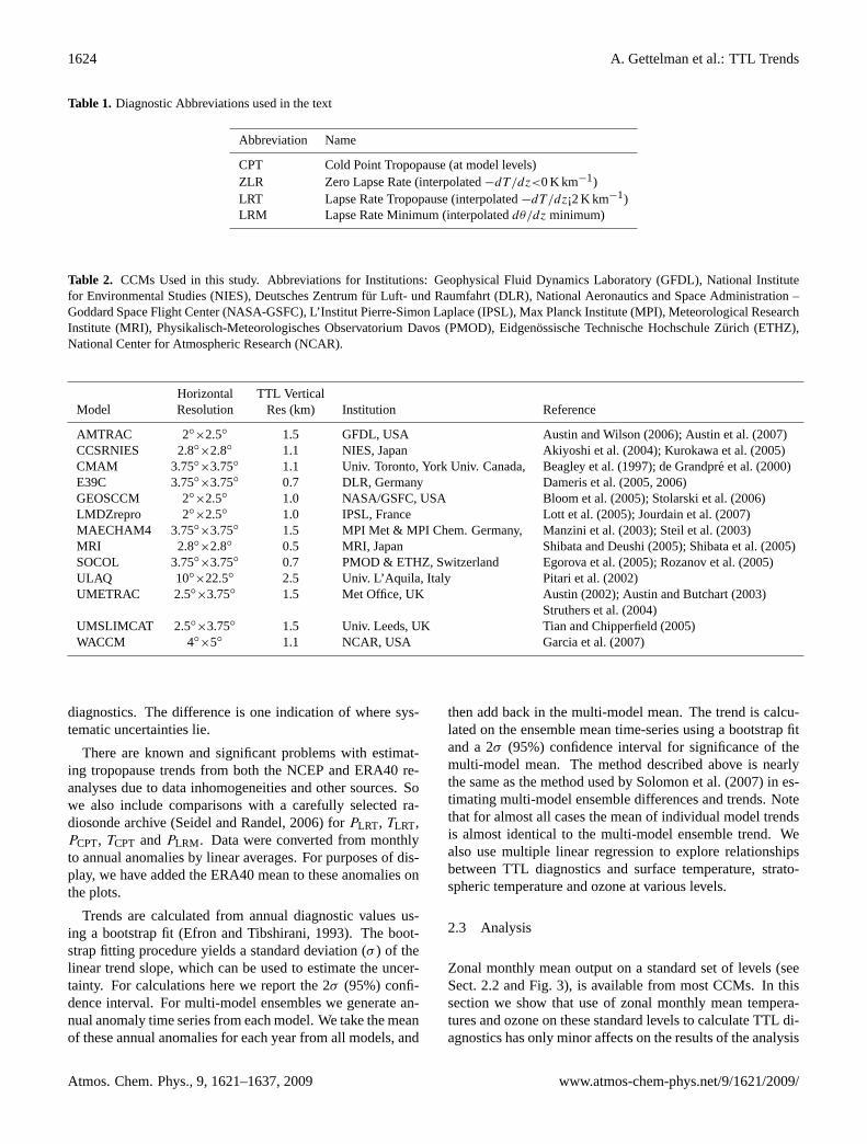
Table 1. Diagnostic Abbreviations used in the text

Abbreviation Name

CPT Cold Point Tropopause (at model levels)ZLR Zero Lapse Rate (interpolated−dT /dz<0 K km−1)LRT Lapse Rate Tropopause (interpolated−dT /dz¡2 K km−1)LRM Lapse Rate Minimum (interpolateddθ/dz minimum)

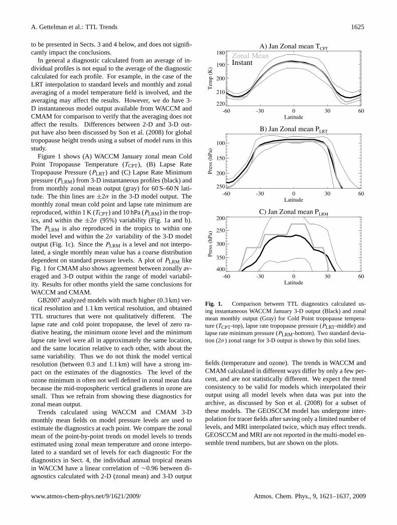
Table 2. CCMs Used in this study. Abbreviations for Institutions: Geophysical Fluid Dynamics Laboratory (GFDL), National Institutefor Environmental Studies (NIES), Deutsches Zentrum fur Luft- und Raumfahrt (DLR), National Aeronautics and Space Administration –Goddard Space Flight Center (NASA-GSFC), L’Institut Pierre-Simon Laplace (IPSL), Max Planck Institute (MPI), Meteorological ResearchInstitute (MRI), Physikalisch-Meteorologisches Observatorium Davos (PMOD), Eidgenossische Technische Hochschule Zurich (ETHZ),National Center for Atmospheric Research (NCAR).

Horizontal TTL VerticalModel Resolution Res (km) Institution Reference

AMTRAC 2◦×2.5◦ 1.5 GFDL, USA Austin and Wilson(2006); Austin et al.(2007)

CCSRNIES 2.8◦×2.8◦ 1.1 NIES, Japan Akiyoshi et al.(2004); Kurokawa et al.(2005)CMAM 3.75◦

×3.75◦ 1.1 Univ. Toronto, York Univ. Canada, Beagley et al.(1997); de Grandpre et al.(2000)E39C 3.75◦×3.75◦ 0.7 DLR, Germany Dameris et al.(2005, 2006)GEOSCCM 2◦×2.5◦ 1.0 NASA/GSFC, USA Bloom et al.(2005); Stolarski et al.(2006)LMDZrepro 2◦×2.5◦ 1.0 IPSL, France Lott et al.(2005); Jourdain et al.(2007)MAECHAM4 3.75◦×3.75◦ 1.5 MPI Met & MPI Chem. Germany, Manzini et al.(2003); Steil et al.(2003)MRI 2.8◦

×2.8◦ 0.5 MRI, Japan Shibata and Deushi(2005); Shibata et al.(2005)SOCOL 3.75◦×3.75◦ 0.7 PMOD & ETHZ, Switzerland Egorova et al.(2005); Rozanov et al.(2005)ULAQ 10◦

×22.5◦ 2.5 Univ. L’Aquila, Italy Pitari et al.(2002)UMETRAC 2.5◦×3.75◦ 1.5 Met Office, UK Austin (2002); Austin and Butchart(2003)

Struthers et al.(2004)UMSLIMCAT 2.5◦

×3.75◦ 1.5 Univ. Leeds, UK Tian and Chipperfield(2005)WACCM 4◦

×5◦ 1.1 NCAR, USA Garcia et al.(2007)

diagnostics. The difference is one indication of where sys-tematic uncertainties lie.

There are known and significant problems with estimat-ing tropopause trends from both the NCEP and ERA40 re-analyses due to data inhomogeneities and other sources. Sowe also include comparisons with a carefully selected ra-diosonde archive (Seidel and Randel, 2006) for PLRT, TLRT,PCPT, TCPT andPLRM . Data were converted from monthlyto annual anomalies by linear averages. For purposes of dis-play, we have added the ERA40 mean to these anomalies onthe plots.

Trends are calculated from annual diagnostic values us-ing a bootstrap fit (Efron and Tibshirani, 1993). The boot-strap fitting procedure yields a standard deviation (σ ) of thelinear trend slope, which can be used to estimate the uncer-tainty. For calculations here we report the 2σ (95%) confi-dence interval. For multi-model ensembles we generate an-nual anomaly time series from each model. We take the meanof these annual anomalies for each year from all models, and

then add back in the multi-model mean. The trend is calcu-lated on the ensemble mean time-series using a bootstrap fitand a 2σ (95%) confidence interval for significance of themulti-model mean. The method described above is nearlythe same as the method used bySolomon et al.(2007) in es-timating multi-model ensemble differences and trends. Notethat for almost all cases the mean of individual model trendsis almost identical to the multi-model ensemble trend. Wealso use multiple linear regression to explore relationshipsbetween TTL diagnostics and surface temperature, strato-spheric temperature and ozone at various levels.

2.3 Analysis

Zonal monthly mean output on a standard set of levels (seeSect.2.2 and Fig.3), is available from most CCMs. In thissection we show that use of zonal monthly mean tempera-tures and ozone on these standard levels to calculate TTL di-agnostics has only minor affects on the results of the analysis



to be presented in Sects.3 and4 below, and does not signifi-cantly impact the conclusions.

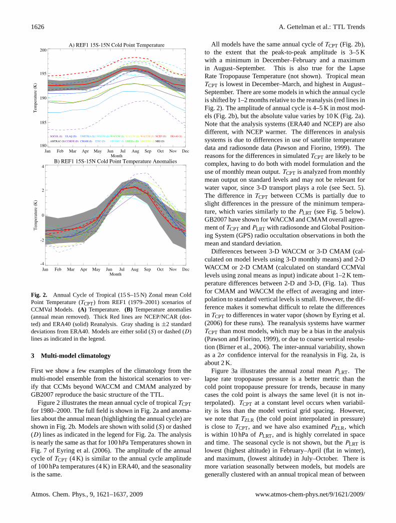
In general a diagnostic calculated from an average of in-dividual profiles is not equal to the average of the diagnosticcalculated for each profile. For example, in the case of theLRT interpolation to standard levels and monthly and zonalaveraging of a model temperature field is involved, and theaveraging may affect the results. However, we do have 3-D instantaneous model output available from WACCM andCMAM for comparison to verify that the averaging does notaffect the results. Differences between 2-D and 3-D out-put have also been discussed bySon et al.(2008) for globaltropopause height trends using a subset of model runs in thisstudy.

Figure 1 shows (A) WACCM January zonal mean ColdPoint Tropopause Temperature (TCPT), (B) Lapse RateTropopause Pressure (PLRT) and (C) Lapse Rate Minimumpressure (PLRM) from 3-D instantaneous profiles (black) andfrom monthly zonal mean output (gray) for 60 S–60 N lati-tude. The thin lines are±2σ in the 3-D model output. Themonthly zonal mean cold point and lapse rate minimum arereproduced, within 1 K (TCPT) and 10 hPa (PLRM) in the trop-ics, and within the±2σ (95%) variability (Fig.1a and b).The PLRM is also reproduced in the tropics to within onemodel level and within the 2σ variability of the 3-D modeloutput (Fig.1c). Since thePLRM is a level and not interpo-lated, a single monthly mean value has a coarse distributiondependent on standard pressure levels. A plot ofPLRM likeFig.1 for CMAM also shows agreement between zonally av-eraged and 3-D output within the range of model variabil-ity. Results for other months yield the same conclusions forWACCM and CMAM.

GB2007 analyzed models with much higher (0.3 km) ver-tical resolution and 1.1 km vertical resolution, and obtainedTTL structures that were not qualitatively different. Thelapse rate and cold point tropopause, the level of zero ra-diative heating, the minimum ozone level and the minimumlapse rate level were all in approximately the same location,and the same location relative to each other, with about thesame variability. Thus we do not think the model verticalresolution (between 0.3 and 1.1 km) will have a strong im-pact on the estimates of the diagnostics. The level of theozone minimum is often not well defined in zonal mean databecause the mid-tropospheric vertical gradients in ozone aresmall. Thus we refrain from showing these diagnostics forzonal mean output.

Trends calculated using WACCM and CMAM 3-Dmonthly mean fields on model pressure levels are used toestimate the diagnostics at each point. We compare the zonalmean of the point-by-point trends on model levels to trendsestimated using zonal mean temperature and ozone interpo-lated to a standard set of levels for each diagnostic For thediagnostics in Sect.4, the individual annual tropical meansin WACCM have a linear correlation of∼0.96 between di-agnostics calculated with 2-D (zonal mean) and 3-D output

Figures

A) Jan Zonal mean TCPT

-60 -30 0 30 60Latitude

220

210

200

190

180

Tem

p (K

)

InstantZonal Mean

C) Jan Zonal mean PLRM

-60 -30 0 30 60Latitude

400

350

300

250

200Pr

ess (

hPa)

B) Jan Zonal mean PLRT

-60 -30 0 30 60Latitude

250

200

150

100

Pres

s (hP

a)

Fig. 1. Comparison between TTL diagnostics calculated using instantaneous WACCM January 3D output(Black) and zonal mean monthly output (Gray) for Cold Point tropopause temperature (TCPT -top), lapse ratetropopause pressure (PLRT -middle) and lapse rate minimum pressure (PLRM -bottom). Two standard deviation(2σ) zonal range for 3D output is shown by thin solid lines.

27

Fig. 1. Comparison between TTL diagnostics calculated us-ing instantaneous WACCM January 3-D output (Black) and zonalmean monthly output (Gray) for Cold Point tropopause tempera-ture (TCPT-top), lapse rate tropopause pressure (PLRT-middle) andlapse rate minimum pressure (PLRM -bottom). Two standard devia-tion (2σ ) zonal range for 3-D output is shown by thin solid lines.

fields (temperature and ozone). The trends in WACCM andCMAM calculated in different ways differ by only a few per-cent, and are not statistically different. We expect the trendconsistency to be valid for models which interpolated theiroutput using all model levels when data was put into thearchive, as discussed bySon et al.(2008) for a subset ofthese models. The GEOSCCM model has undergone inter-polation for tracer fields after saving only a limited number oflevels, and MRI interpolated twice, which may effect trends.GEOSCCM and MRI are not reported in the multi-model en-semble trend numbers, but are shown on the plots.



A) REF1 15S-15N Cold Point Temperature

Jan Feb Mar Apr May Jun Jul Aug Sep Oct Nov DecMonth

180

185

190

195

200

Tem

pera

ture

(K)

AMTRAC (S) CCSRNI (D) CMAM (S) E39C (D) GEOSCC (S) LMDZre (D) MAECHA (S)MRI (D)

SOCOL (S) ULAQ (D) UMETRA (S) UMSLIM (D) WACCM (S) WACCM (D) WACCM (S) NCEP (D) ERA40 (S)

B) REF1 15S-15N Cold Point Temperature Anomalies


-4

-2

0

2

4

Tem

pera

ture

(K)

Fig. 2. Annual Cycle of Tropical (15S-15N) Zonal mean Cold Point Temperature (TCPT ) from REF1 (1979–2001) scenarios of CCMVal Models. A) Temperature. B) Temperature anomalies (annual mean removed).Thick Red lines are NCEP/NCAR (dotted) and ERA40 (solid) Reanalysis. Gray shading is ±2 standard devia-tions from ERA40. Models are either solid (S) or dashed (D) lines as indicated in the legend.

28

A) REF1 15S-15N Cold Point Temperature


180

185

190

195

200

Tem

pera

ture

(K)

AMTRAC (S) CCSRNI (D) CMAM (S) E39C (D) GEOSCC (S) LMDZre (D) MAECHA (S)MRI (D)


B) REF1 15S-15N Cold Point Temperature Anomalies


-4

-2

0

2

4

Tem

pera

ture

(K)

Fig. 2. Annual Cycle of Tropical (15S-15N) Zonal mean Cold Point Temperature (TCPT ) from REF1 (1979–2001) scenarios of CCMVal Models. A) Temperature. B) Temperature anomalies (annual mean removed).Thick Red lines are NCEP/NCAR (dotted) and ERA40 (solid) Reanalysis. Gray shading is ±2 standard devia-tions from ERA40. Models are either solid (S) or dashed (D) lines as indicated in the legend.

28

Fig. 2. Annual Cycle of Tropical (15 S–15 N) Zonal mean ColdPoint Temperature (TCPT) from REF1 (1979–2001) scenarios ofCCMVal Models. (A) Temperature.(B) Temperature anomalies(annual mean removed). Thick Red lines are NCEP/NCAR (dot-ted) and ERA40 (solid) Reanalysis. Gray shading is±2 standarddeviations from ERA40. Models are either solid (S) or dashed (D)lines as indicated in the legend.

3 Multi-model climatology

First we show a few examples of the climatology from themulti-model ensemble from the historical scenarios to ver-ify that CCMs beyond WACCM and CMAM analyzed byGB2007 reproduce the basic structure of the TTL.

Figure2 illustrates the mean annual cycle of tropicalTCPTfor 1980–2000. The full field is shown in Fig.2a and anoma-lies about the annual mean (highlighting the annual cycle) areshown in Fig.2b. Models are shown with solid (S) or dashed(D) lines as indicated in the legend for Fig.2a. The analysisis nearly the same as that for 100 hPa Temperatures shown inFig. 7 of Eyring et al.(2006). The amplitude of the annualcycle ofTCPT (4 K) is similar to the annual cycle amplitudeof 100 hPa temperatures (4 K) in ERA40, and the seasonalityis the same.

All models have the same annual cycle ofTCPT (Fig. 2b),to the extent that the peak-to-peak amplitude is 3–5 Kwith a minimum in December–February and a maximumin August–September. This is also true for the LapseRate Tropopause Temperature (not shown). Tropical meanTCPT is lowest in December–March, and highest in August–September. There are some models in which the annual cycleis shifted by 1–2 months relative to the reanalysis (red lines inFig.2). The amplitude of annual cycle is 4–5 K in most mod-els (Fig.2b), but the absolute value varies by 10 K (Fig.2a).Note that the analysis systems (ERA40 and NCEP) are alsodifferent, with NCEP warmer. The differences in analysissystems is due to differences in use of satellite temperaturedata and radiosonde data (Pawson and Fiorino, 1999). Thereasons for the differences in simulatedTCPT are likely to becomplex, having to do both with model formulation and theuse of monthly mean output.TCPT is analyzed from monthlymean output on standard levels and may not be relevant forwater vapor, since 3-D transport plays a role (see Sect.5).The difference inTCPT between CCMs is partially due toslight differences in the pressure of the minimum tempera-ture, which varies similarly to thePLRT (see Fig.5 below).GB2007 have shown for WACCM and CMAM overall agree-ment ofTCPT andPLRT with radiosonde and Global Position-ing System (GPS) radio occultation observations in both themean and standard deviation.

Differences between 3-D WACCM or 3-D CMAM (cal-culated on model levels using 3-D monthly means) and 2-DWACCM or 2-D CMAM (calculated on standard CCMVallevels using zonal means as input) indicate about 1–2 K tem-perature differences between 2-D and 3-D, (Fig.1a). Thusfor CMAM and WACCM the effect of averaging and inter-polation to standard vertical levels is small. However, the dif-ference makes it somewhat difficult to relate the differencesin TCPT to differences in water vapor (shown byEyring et al.(2006) for these runs). The reanalysis systems have warmerTCPT than most models, which may be a bias in the analysis(Pawson and Fiorino, 1999), or due to coarse vertical resolu-tion (Birner et al., 2006). The inter-annual variability, shownas a 2σ confidence interval for the reanalysis in Fig.2a, isabout 2 K.

Figure 3a illustrates the annual zonal meanPLRT. Thelapse rate tropopause pressure is a better metric than thecold point tropopause pressure for trends, because in manycases the cold point is always the same level (it is not in-terpolated).TCPT at a constant level occurs when variabil-ity is less than the model vertical grid spacing. However,we note thatTZLR (the cold point interpolated in pressure)is close toTCPT, and we have also examinedPZLR, whichis within 10 hPa ofPLRT, and is highly correlated in spaceand time. The seasonal cycle is not shown, but thePLRT islowest (highest altitude) in February–April (flat in winter),and maximum, (lowest altitude) in July–October. There ismore variation seasonally between models, but models aregenerally clustered with an annual tropical mean of between



92–102 hPa (PLRT is interpolated) and an annual cycle am-plitude of about 10 hPa. There is more variation betweenmodels poleward of 30◦ latitude.

The PLRM is illustrated in Fig.3b. PLRM is generallyaround 250 hPa in the deep tropics (15 S–15 N latitude), with2 models near 200 hPa, and scatter below this. There is lit-tle annual cycle in most models (not shown).PLRM is welldefined in convective regions (see GB2007 for more details)within ∼20◦ of the equator. It is not well defined outside ofthe deep tropics and is not a useful diagnostic there.

4 Long term trends

As noted in Sect.2.3we have analyzed trends from WACCMand CMAM with both 3-D and zonal monthly mean data, andfound no significant differences inPLRT, TCPT or PLRM . ForWACCM the correlation between 3-D and 2-D annual meansis ∼0.96. So for estimating trends, we use the zonal monthlymean data available from all the models. We start with his-torical trends (REF1: 1960–2001) in Sect.4.1 and then dis-cuss scenarios for the future in Sect.4.2. Table3 summarizesmulti-model and observed trends for various quantities, withstatistical significance (indicated by an asterisk in the table)based on the 2σ (95%) confidence intervals from a bootstrapfit of the multi-model ensemble mean time-series. For thelast three columns, not all models provide output over theentire time period (see for example, Fig.4). Eleven mod-els are included in statistics for REF1 and nine for REF2.E39C and UMETRAC REF2 runs were not available, andthe GEOSCCM and MRI values were not included due todouble interpolation. ULAQ is not included for analysis ofPLRM due to resolution.

4.1 Historical trends

Little change is evident from 1960–2005 in simulatedTCPT(Fig. 4). It is hard to find any trends which are significantlydifferent from zero in the simulations (Table3). Some mod-els appear to cool, some to warm, but these do not appear tobe significant trends. However, many models and the reanal-ysis systems do indicate cooling from 1991–2004. The resultis consistent with Fig. 2 ofEyring et al.(2007) that shows thevertical structure of tropical temperature trends. There is asignificant negative trend inTCPT estimated from radiosondeanalyses. NCEP reproduces the trend, but ERA40 does not.However, the NCEP trend may be spurious (Randel et al.(2006), and references therein) resulting from changes in in-put data over time. Thus there is also significant uncertaintyin TCPT trends in the reanalysis data. Radiosonde trends areconsidered more robust (Seidel and Randel, 2006).

The Lapse Rate Tropopause Pressure (PLRT) does appearto decrease in the simulations (Fig.5) and in the reanalyzes,indicating a lower pressure (higher altitude) to the tropicaltropopause of−1 to −1.5 hPa/decade (Table3). However,

A) Annual Lapse Rate Trop Pressure

-60 -40 -20 0 20 40 60Latitude

400

300250

2001701501301151009080

Pres

sure

(hPa

) AMTRAC (S)CCSRNIES (D)CMAM (S)E39C (D)GEOSCCM (S)LMDZrepro (D)MAECHAM4CHEM (S)MRI (D)SOCOL (S)ULAQ (D)UMETRAC (S)UMSLIMCAT (D)WACCM (S)WACCM (D)WACCM (S)NCEP (D)ERA40 (S)

B) Annual Lapse Rate Min Pressure

-60 -40 -20 0 20 40 60Latitude

500

400

300

250

200

170

Pres

sure

(hPa

)

Fig. 3. Zonal mean (A) Lapse Rate Tropopause Pressure (PLRT ) and (B) Lapse Rate Minimum Pressure(PLRM ) from CCMVal models (REF1 scenarios, 1979–2001). Thick Red lines are NCEP/NCAR (dashed) andERA40 (solid) Reanalyses. Models are either solid (S) or dashed (D) lines as indicated in the legend in (A).Vertical levels used are noted by tick marks on the vertical axis.

29

A) Annual Lapse Rate Trop Pressure

-60 -40 -20 0 20 40 60Latitude

400

300250

2001701501301151009080

Pres

sure

(hPa

) AMTRAC (S)CCSRNIES (D)CMAM (S)E39C (D)GEOSCCM (S)LMDZrepro (D)MAECHAM4CHEM (S)MRI (D)SOCOL (S)ULAQ (D)UMETRAC (S)UMSLIMCAT (D)WACCM (S)WACCM (D)WACCM (S)NCEP (D)ERA40 (S)

B) Annual Lapse Rate Min Pressure

-60 -40 -20 0 20 40 60Latitude

500

400

300

250

200

170

Pres

sure

(hPa

)

Fig. 3. Zonal mean (A) Lapse Rate Tropopause Pressure (PLRT ) and (B) Lapse Rate Minimum Pressure(PLRM ) from CCMVal models (REF1 scenarios, 1979–2001). Thick Red lines are NCEP/NCAR (dashed) andERA40 (solid) Reanalyses. Models are either solid (S) or dashed (D) lines as indicated in the legend in (A).Vertical levels used are noted by tick marks on the vertical axis.

29

Fig. 3. Zonal mean(A) Lapse Rate Tropopause Pressure (PLRT)and (B) Lapse Rate Minimum Pressure (PLRM ) from CCM-Val models (REF1 scenarios, 1979–2001). Thick Red lines areNCEP/NCAR (dashed) and ERA40 (solid) Reanalyses. Models areeither solid (S) or dashed (D) lines as indicated in the legend in (A).Vertical levels used are noted by tick marks on the vertical axis.

there is no trend in radiosonde analyses ofPLRT from 1979–2001. Other analyses with the Parallel Climate Model (San-ter et al., 2003), a subset of these models (Son et al., 2008)and observations (Seidel et al., 2001; Gettelman and Forster,2002) do show decreases inPLRT. SimulatedPLRT trends areof the same sign and magnitude asPZLR trends. In generalthe trend is consistent across models in Fig.5. Inter-annualvariability in any model is generally less than in the reanal-yses or radiosondes. As noted,TCPT is correlated with CPTpressure. The correlation can be seen in thePLRT as well inFig. 5: models with lower pressurePLRT have lowerTCPT(Fig. 4).

These tropopause changes represent changes in the “top”of the TTL. The “bottom” of the TTL is represented by theLapse Rate Minimum pressure (PLRM), which is related to



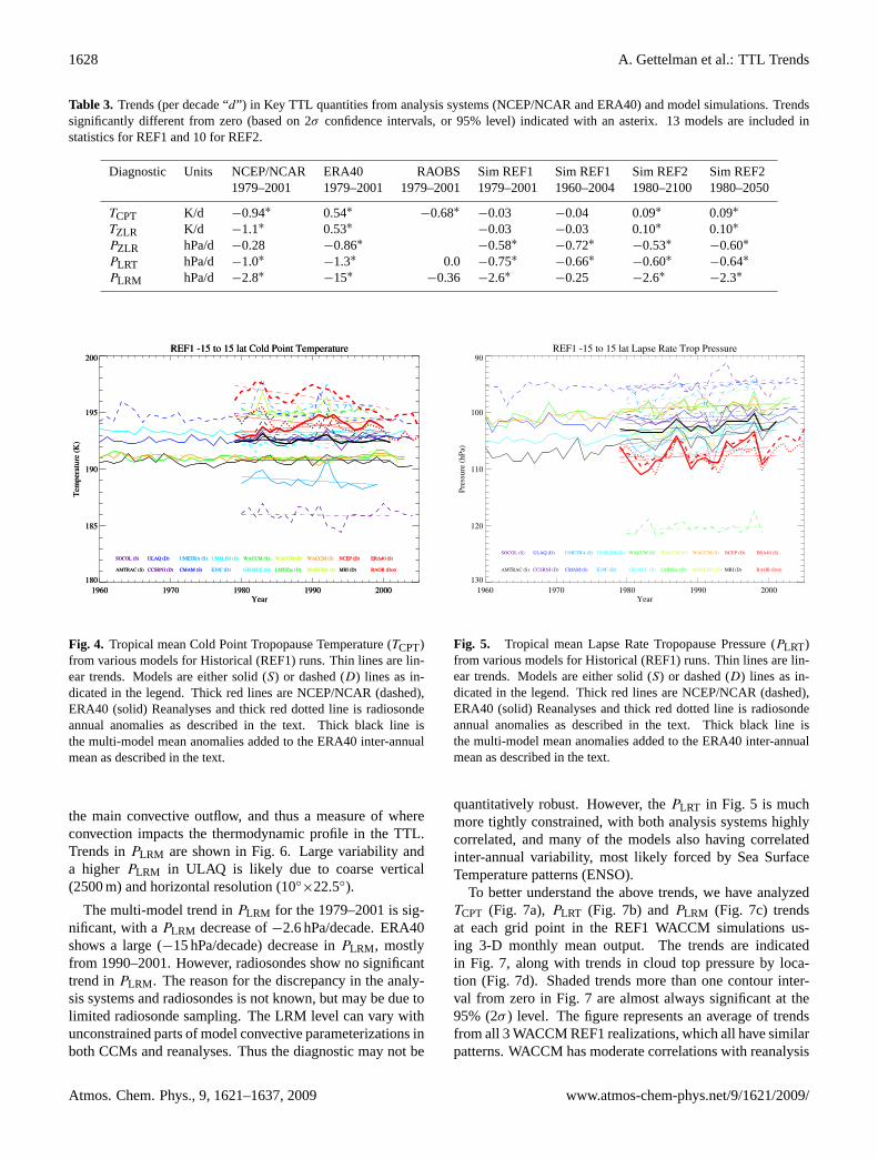
Table 3. Trends (per decade “d”) in Key TTL quantities from analysis systems (NCEP/NCAR and ERA40) and model simulations. Trendssignificantly different from zero (based on 2σ confidence intervals, or 95% level) indicated with an asterix. 13 models are included instatistics for REF1 and 10 for REF2.

Diagnostic Units NCEP/NCAR ERA40 RAOBS Sim REF1 Sim REF1 Sim REF2 Sim REF21979–2001 1979–2001 1979–2001 1979–2001 1960–2004 1980–2100 1980–2050

TCPT K/d −0.94∗ 0.54∗ −0.68∗ −0.03 −0.04 0.09∗ 0.09∗

TZLR K/d −1.1∗ 0.53∗ −0.03 −0.03 0.10∗ 0.10∗

PZLR hPa/d −0.28 −0.86∗ −0.58∗ −0.72∗ −0.53∗ −0.60∗

PLRT hPa/d −1.0∗ −1.3∗ 0.0 −0.75∗ −0.66∗ −0.60∗ −0.64∗

PLRM hPa/d −2.8∗ −15∗−0.36 −2.6∗ −0.25 −2.6∗ −2.3∗

REF1 -15 to 15 lat Cold Point Temperature

1960 1970 1980 1990 2000Year

180

185

190

195

200

Tem

pera

ture

(K)

AMTRAC (S) CCSRNI (D) CMAM (S) E39C (D) GEOSCC (S) LMDZre (D) MAECHA (S) MRI (D)


RAOB (Dot)


1960 1970 1980 1990 2000Year

180

185

190

195

200

Tem

pera

ture

(K)



RAOB (Dot)

Fig. 4. Tropical mean Cold Point Tropopause Temperature (TCPT ) from various models for Historical (REF1)runs. Thin lines are linear trends. Models are either solid (S) or dashed (D) lines as indicated in the legend.Thick red lines are NCEP/NCAR (dashed), ERA40 (solid) Reanalyses and thick red dotted line is radiosondeannual anomalies as described in the text. Thick black line is the multi-model mean anomalies added to theERA40 inter-annual mean as described in the text.

30

Fig. 4. Tropical mean Cold Point Tropopause Temperature (TCPT)from various models for Historical (REF1) runs. Thin lines are lin-ear trends. Models are either solid (S) or dashed (D) lines as in-dicated in the legend. Thick red lines are NCEP/NCAR (dashed),ERA40 (solid) Reanalyses and thick red dotted line is radiosondeannual anomalies as described in the text. Thick black line isthe multi-model mean anomalies added to the ERA40 inter-annualmean as described in the text.

the main convective outflow, and thus a measure of whereconvection impacts the thermodynamic profile in the TTL.Trends inPLRM are shown in Fig.6. Large variability anda higherPLRM in ULAQ is likely due to coarse vertical(2500 m) and horizontal resolution (10◦

×22.5◦).

The multi-model trend inPLRM for the 1979–2001 is sig-nificant, with aPLRM decrease of−2.6 hPa/decade. ERA40shows a large (−15 hPa/decade) decrease inPLRM , mostlyfrom 1990–2001. However, radiosondes show no significanttrend inPLRM . The reason for the discrepancy in the analy-sis systems and radiosondes is not known, but may be due tolimited radiosonde sampling. The LRM level can vary withunconstrained parts of model convective parameterizations inboth CCMs and reanalyses. Thus the diagnostic may not be

REF1 -15 to 15 lat Lapse Rate Trop Pressure

1960 1970 1980 1990 2000Year

130

120

110

100

90

Pres

sure

(hPa

)



RAOB (Dot)

Fig. 5. Tropical mean Lapse Rate Tropopause Pressure (PLRT ) from various models for Historical (REF1)runs. Thin lines are linear trends. Models are either solid (S) or dashed (D) lines as indicated in the legend.Thick red lines are NCEP/NCAR (dashed), ERA40 (solid) Reanalyses and thick red dotted line is radiosondeannual anomalies as described in the text. Thick black line is the multi-model mean anomalies added to theERA40 inter-annual mean as described in the text.

31

Fig. 5. Tropical mean Lapse Rate Tropopause Pressure (PLRT)from various models for Historical (REF1) runs. Thin lines are lin-ear trends. Models are either solid (S) or dashed (D) lines as in-dicated in the legend. Thick red lines are NCEP/NCAR (dashed),ERA40 (solid) Reanalyses and thick red dotted line is radiosondeannual anomalies as described in the text. Thick black line isthe multi-model mean anomalies added to the ERA40 inter-annualmean as described in the text.

quantitatively robust. However, thePLRT in Fig. 5 is muchmore tightly constrained, with both analysis systems highlycorrelated, and many of the models also having correlatedinter-annual variability, most likely forced by Sea SurfaceTemperature patterns (ENSO).

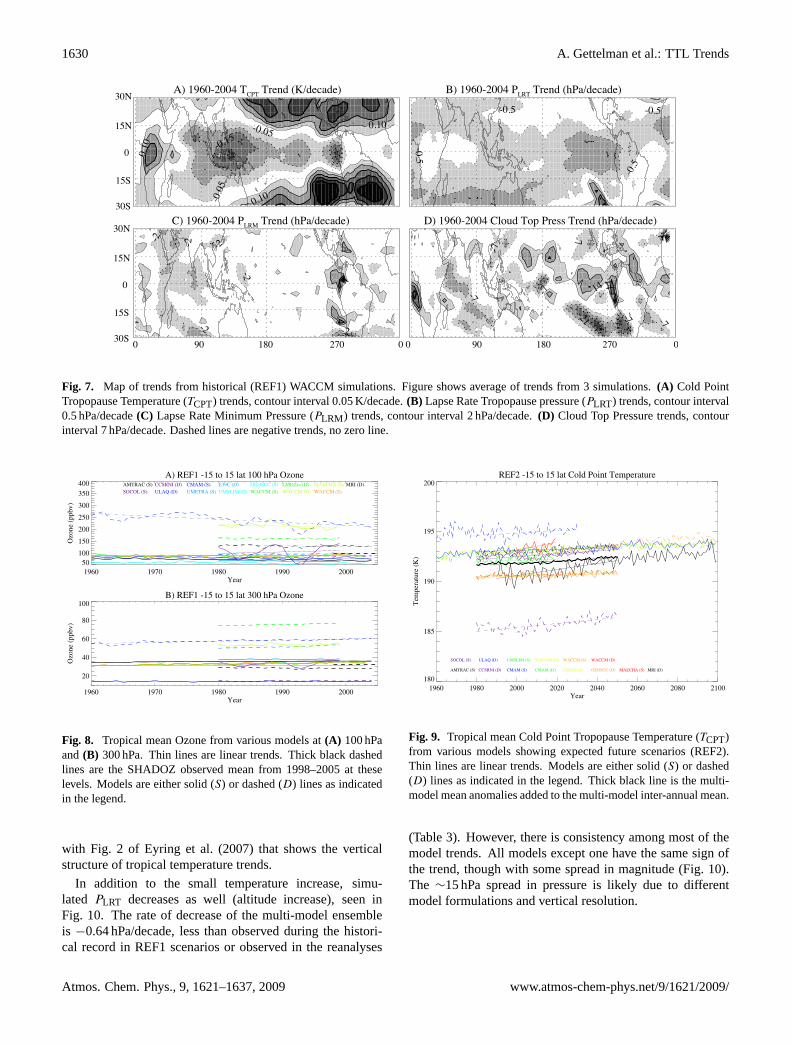
To better understand the above trends, we have analyzedTCPT (Fig. 7a), PLRT (Fig. 7b) andPLRM (Fig. 7c) trendsat each grid point in the REF1 WACCM simulations us-ing 3-D monthly mean output. The trends are indicatedin Fig. 7, along with trends in cloud top pressure by loca-tion (Fig. 7d). Shaded trends more than one contour inter-val from zero in Fig.7 are almost always significant at the95% (2σ ) level. The figure represents an average of trendsfrom all 3 WACCM REF1 realizations, which all have similarpatterns. WACCM has moderate correlations with reanalysis



PLRT (Fig.5), but with less inter-annual variability. WACCMhas less variability because it does not include the aerosol ef-fects of significant volcanic eruptions (such as Mt. Pinatuboin 1991 or El Chichon in 1983).

In Fig. 7a simulatedTCPT decreases throughout the trop-ics in WACCM and increases in the subtropics. WACCMsimulatedTCPT changes are largest centered over the West-ern Pacific, but simulatedTCPT actually increases over Trop-ical Africa. The simulated zonal mean trend is not signif-icant. These changes can be partially explained with thepattern of changes in simulated cloud top pressure (Fig.7d)in WACCM, with decreasing pressure (higher clouds) in theWestern Pacific and increasing pressure (lower clouds) in theEastern Pacific. The clouds appear to shift towards the equa-tor from the South Pacific Convergence Zone (SPCZ), withincreasing cloud pressure north of Australia in the WACCMsimulations. Figure7b shows that the simulatedPLRT hasdecreased almost everywhere in the tropics and sub-tropics,with largest changes in the Eastern Pacific. SimulatedPLRM(Fig. 7c) does not have a coherent trend in WACCM, consis-tent with Fig.6.

There are very large differences in mean 300 hPa ozonein the tropical troposphere in the models (Fig.8b). 300 hPais a level near the ozone minimum. The differences are ex-pected since tropospheric ozone boundary conditions werenot specified, and the models have different representationsof tropospheric chemistry. The spread of ozone at 300 hPa is10–80 ppbv with most models clustered around the observedvalue of 30 ppbv (from SHADOZ Ozonezondes). CMAMozone (the lowest) is low due to a lack of tropospheric ozonesources or chemistry which may impactTCPT.

Even at 100 hPa near the tropopause there are variations inozone between 75–300 ppbv (Fig.8a). The values get largerthan the∼120 ppbv observed from SHADOZ. Most mod-els have a low bias relative to SHADOZ. Several models arenot clustered with the others in Fig.8a, including LMDZ,MAECHAM, MRI, SOCOL and ULAQ. For MAECHAMthis is related to low ascent rates in the lower stratosphere(Steil et al., 2003). There is also a positive correlation(linear correlation coefficient∼0.6) between average ColdPoint Temperature and average ozone in models around thetropopause (150–70 hPa). Models with higher ozone havehigher tropopause temperatures in Fig.2, consistent withan important role for ozone in the radiative heating of theTTL. It may also result from differences in dynamical pro-cesses (slower uplift would imply both higher temperaturesand higher ozone). We discuss this further in Sect.5.

4.2 Future scenarios

We now examine the evolution of the TTL for the futurescenario (REF2). As discussed inEyring et al. (2007),the future scenario uses near common forcing for all mod-els. Models were run from 1960 or 1980 to 2050 or2100. Surface concentrations of greenhouse gases (CO2,

REF1 -15 to 15 lat Lapse Rate Min Pressure

1960 1970 1980 1990 2000Year

350

300

250

200

Pres

sure

(hPa

)



RAOB (Dot)

Fig. 6. Tropical mean Lapse Rate Minimum Pressure (PLRM ) from various models for Historical (REF1) runs.Thin lines are linear trends. Models are either solid (S) or dashed (D) lines as indicated in the legend. Thickred lines are NCEP/NCAR (dashed), ERA40 (solid) Reanalyses and thick red dotted line is radiosonde annualanomalies as described in the text. Thick black line is the multi-model mean anomalies added to the ERA40inter-annual mean as described in the text.

32

Fig. 6. Tropical mean Lapse Rate Minimum Pressure (PLRM ) fromvarious models for Historical (REF1) runs. Thin lines are lineartrends. Models are either solid (S) or dashed (D) lines as indicatedin the legend. Thick red lines are NCEP/NCAR (dashed), ERA40(solid) Reanalyses and thick red dotted line is radiosonde annualanomalies as described in the text. Thick black line is the multi-model mean anomalies added to the ERA40 inter-annual mean asdescribed in the text.

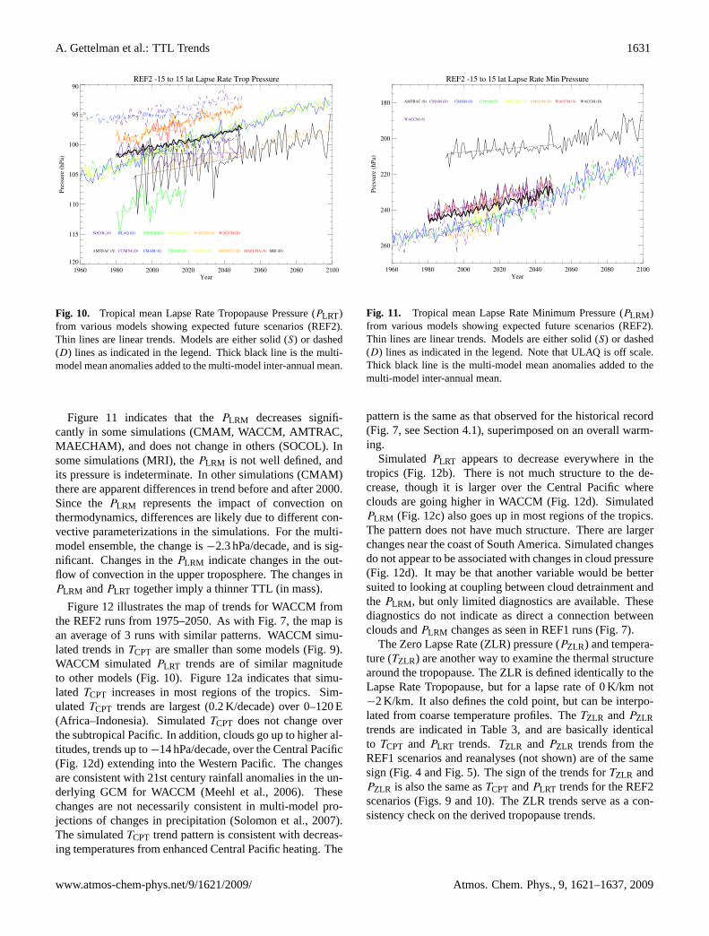
CH4, N2O) are specified from the Intergovernmental Panelon Climate Change (IPCC) Special Report on EmissionsScenarios (SRES) GHG scenario A1b (medium) (IPCC,2000). Surface halogens (chlorofluorocarbons (CFCs),hydro-chlorofluorocarbons (HCFCs), and halons) are pre-scribed according to the A1b scenario ofWorld Meteorolog-ical Organization(2003). Sea surface temperatures (SSTs)and sea ice distributions are derived from IPCC 4th Assess-ment Report simulations with the coupled ocean-atmospheremodels upon which the CCMs are based. Otherwise, SSTsand sea ice distributions are from a simulation with the UKMet Office Hadley Centre coupled ocean-atmosphere modelHadGEM1 (Johns et al., 2006). SeeEyring et al.(2007) fordetails. Trends in Table3 are calculated from available datafor each model from 1980 to 2050, since only 3 CCMs (AM-TRAC, CMAM, GEOSCCM) are run to 2100. Future trendsare broadly linear, and trends for those models run to 2100are not significantly different if the period 1980–2100 is used(the last two columns are nearly identical. Trends are slightlylarger for 2000–2050, likely due to additional forcing fromozone recovery.

Figure9 illustrates changes inTCPT, similar to Fig.4 butfor the future (REF2) scenario. Models generally projectcold point or lapse rate tropopause temperatures to increaseslightly. The multi-model rate of temperature increase is only0.09 K/decade (Table3), but is significant. For AMTRAC,the increase is almost 0.3 K/decade in the early part of the21st century. The increase may be related to the low ozone atthe tropopause (Son et al., 2008). The analysis is consistent



A) 1960-2004 TCPT

Trend (K/decade)

-0.15

-0.0

5

-0.05

0.10

0.10

0.1

0

B) 1960-2004 PLRT

Trend (hPa/decade)

-0.5

-0.5-0.5

-0.5

C) 1960-2004 PLRM

Trend (hPa/decade)

-2

-2

-2

-2

-2

-2

4

D) 1960-2004 Cloud Top Press Trend (hPa/decade)-21

-7

-7 -7

-7

-7

-7

14

14

30N

30S

15N

15S

0

30N

30S

15N

15S

0

0 90 180 270 0 0 90 180 270 0

Fig. 7. Map of trends from historical (REF1) WACCM simulations. Figure shows average of trends from 3simulations. A) Cold Point Tropopause Temperature (TCPT ) trends, contour interval 0.05K/decade. B) LapseRate Tropopause pressure (PLRT ) trends, contour interval 0.5hPa/decade C) Lapse Rate Minimum Pressure(PLRM ) trends, contour interval 2hPa/decade. D) Cloud Top Pressure trends, contour interval 7hPa/decade.Dashed lines are negative trends, no zero line.

A) REF1 -15 to 15 lat 100 hPa Ozone

1960 1970 1980 1990 2000Year

50100150200250300350400

Ozo

ne (p

pbv)

AMTRAC (S) CCSRNI (D) CMAM (S) E39C (D) GEOSCC (S) LMDZre (D) MAECHA (S) MRI (D)SOCOL (S) ULAQ (D) UMETRA (S) UMSLIM (D) WACCM (S) WACCM (D) WACCM (S)

B) REF1 -15 to 15 lat 300 hPa Ozone

1960 1970 1980 1990 2000Year

20

40

60

80

100

Ozo

ne (p

pbv)

Fig. 8. Tropical mean Ozone from various models at (A) 100hPa and (B)300hPa. Thin lines are linear trends.Thick black dashed lines are the SHADOZ observed mean from 1998-2005 at these levels. Models are eithersolid (S) or dashed (D) lines as indicated in the legend.

33

Fig. 7. Map of trends from historical (REF1) WACCM simulations. Figure shows average of trends from 3 simulations.(A) Cold PointTropopause Temperature (TCPT) trends, contour interval 0.05 K/decade.(B) Lapse Rate Tropopause pressure (PLRT) trends, contour interval0.5 hPa/decade(C) Lapse Rate Minimum Pressure (PLRM ) trends, contour interval 2 hPa/decade.(D) Cloud Top Pressure trends, contourinterval 7 hPa/decade. Dashed lines are negative trends, no zero line.

A) 1960-2004 TCPT

Trend (K/decade)

-0.15

-0.0

5

-0.05

0.10

0.10

0.1

0

B) 1960-2004 PLRT

Trend (hPa/decade)

-0.5

-0.5-0.5

-0.5

C) 1960-2004 PLRM

Trend (hPa/decade)

-2

-2

-2

-2

-2

-2

4

D) 1960-2004 Cloud Top Press Trend (hPa/decade)

-21

-7

-7 -7

-7

-7

-7

14

14

30N

30S

15N

15S

0

30N

30S

15N

15S

0

0 90 180 270 0 0 90 180 270 0

Fig. 7. Map of trends from historical (REF1) WACCM simulations. Figure shows average of trends from 3simulations. A) Cold Point Tropopause Temperature (TCPT ) trends, contour interval 0.05K/decade. B) LapseRate Tropopause pressure (PLRT ) trends, contour interval 0.5hPa/decade C) Lapse Rate Minimum Pressure(PLRM ) trends, contour interval 2hPa/decade. D) Cloud Top Pressure trends, contour interval 7hPa/decade.Dashed lines are negative trends, no zero line.

A) REF1 -15 to 15 lat 100 hPa Ozone

1960 1970 1980 1990 2000Year

50100150200250300350400

Ozo

ne (p

pbv)

AMTRAC (S) CCSRNI (D) CMAM (S) E39C (D) GEOSCC (S) LMDZre (D) MAECHA (S) MRI (D)SOCOL (S) ULAQ (D) UMETRA (S) UMSLIM (D) WACCM (S) WACCM (D) WACCM (S)

B) REF1 -15 to 15 lat 300 hPa Ozone

1960 1970 1980 1990 2000Year

20

40

60

80

100

Ozo

ne (p

pbv)

Fig. 8. Tropical mean Ozone from various models at (A) 100hPa and (B)300hPa. Thin lines are linear trends.Thick black dashed lines are the SHADOZ observed mean from 1998-2005 at these levels. Models are eithersolid (S) or dashed (D) lines as indicated in the legend.

33

Fig. 8. Tropical mean Ozone from various models at(A) 100 hPaand(B) 300 hPa. Thin lines are linear trends. Thick black dashedlines are the SHADOZ observed mean from 1998–2005 at theselevels. Models are either solid (S) or dashed (D) lines as indicatedin the legend.

with Fig. 2 of Eyring et al.(2007) that shows the verticalstructure of tropical temperature trends.

In addition to the small temperature increase, simu-lated PLRT decreases as well (altitude increase), seen inFig. 10. The rate of decrease of the multi-model ensembleis −0.64 hPa/decade, less than observed during the histori-cal record in REF1 scenarios or observed in the reanalyses


1960 1980 2000 2020 2040 2060 2080 2100Year

180

185

190

195

200

Tem

pera

ture

(K)

AMTRAC (S) CCSRNI (D) CMAM (S) CMAM (D) CMAM (S) GEOSCC (D) MAECHA (S) MRI (D)

SOCOL (S) ULAQ (D) UMSLIM (S) WACCM (D) WACCM (S) WACCM (D)

Fig. 9. Tropical mean Cold Point Tropopause Temperature (TCPT ) from various models showing expectedfuture scenarios (REF2). Thin lines are linear trends. Models are either solid (S) or dashed (D) lines as indicatedin the legend. Thick black line is the multi-model mean anomalies added to the multi-model inter-annual mean.

34

Fig. 9. Tropical mean Cold Point Tropopause Temperature (TCPT)from various models showing expected future scenarios (REF2).Thin lines are linear trends. Models are either solid (S) or dashed(D) lines as indicated in the legend. Thick black line is the multi-model mean anomalies added to the multi-model inter-annual mean.

(Table3). However, there is consistency among most of themodel trends. All models except one have the same sign ofthe trend, though with some spread in magnitude (Fig.10).The ∼15 hPa spread in pressure is likely due to differentmodel formulations and vertical resolution.



REF2 -15 to 15 lat Lapse Rate Trop Pressure

1960 1980 2000 2020 2040 2060 2080 2100Year

120

115

110

105

100

95

90

Pres

sure

(hPa

)

AMTRAC (S) CCSRNI (D) CMAM (S) CMAM (D) CMAM (S) GEOSCC (D) MAECHA (S) MRI (D)

SOCOL (S) ULAQ (D) UMSLIM (S) WACCM (D) WACCM (S) WACCM (D)

Fig. 10. Tropical mean Lapse Rate Tropopause Pressure (PLRT ) from various models showing expected futurescenarios (REF2). Thin lines are linear trends. Models are either solid (S) or dashed (D) lines as indicated inthe legend. Thick black line is the multi-model mean anomalies added to the multi-model inter-annual mean.

35

Fig. 10. Tropical mean Lapse Rate Tropopause Pressure (PLRT)from various models showing expected future scenarios (REF2).Thin lines are linear trends. Models are either solid (S) or dashed(D) lines as indicated in the legend. Thick black line is the multi-model mean anomalies added to the multi-model inter-annual mean.

Figure 11 indicates that thePLRM decreases signifi-cantly in some simulations (CMAM, WACCM, AMTRAC,MAECHAM), and does not change in others (SOCOL). Insome simulations (MRI), thePLRM is not well defined, andits pressure is indeterminate. In other simulations (CMAM)there are apparent differences in trend before and after 2000.Since thePLRM represents the impact of convection onthermodynamics, differences are likely due to different con-vective parameterizations in the simulations. For the multi-model ensemble, the change is−2.3 hPa/decade, and is sig-nificant. Changes in thePLRM indicate changes in the out-flow of convection in the upper troposphere. The changes inPLRM andPLRT together imply a thinner TTL (in mass).

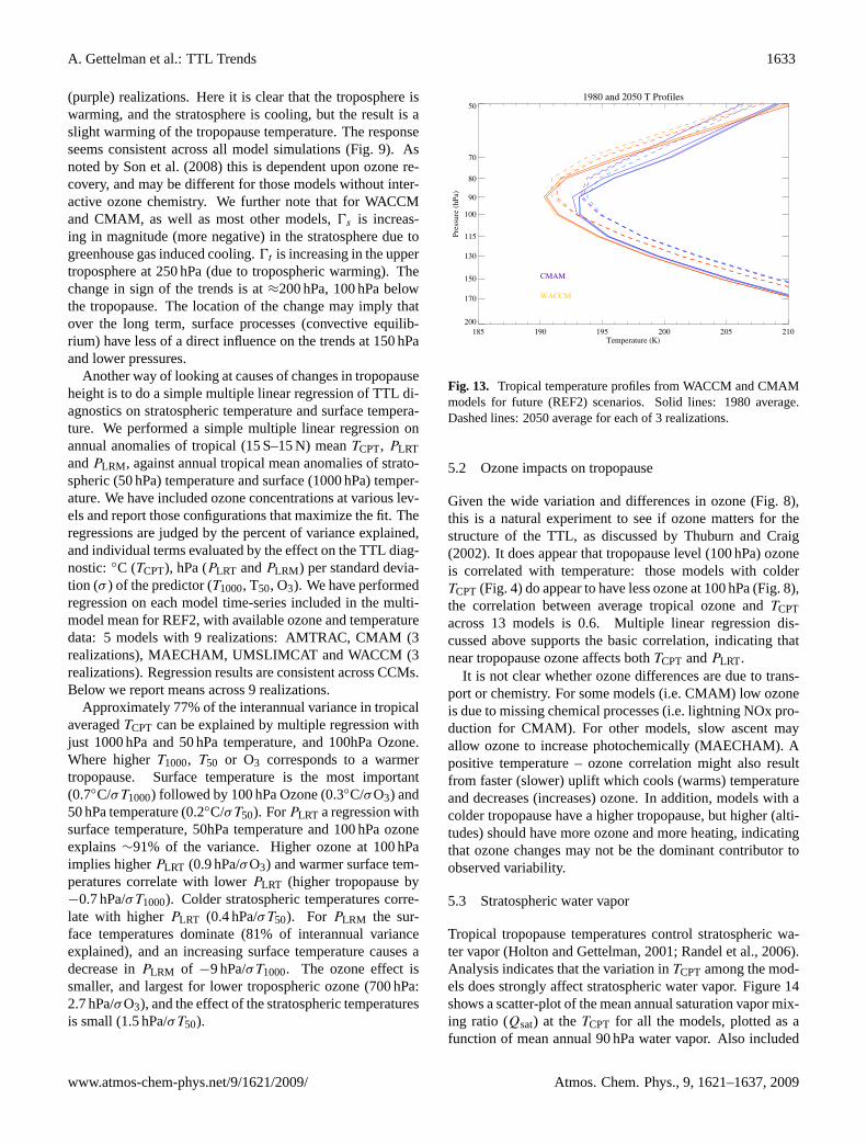
Figure12 illustrates the map of trends for WACCM fromthe REF2 runs from 1975–2050. As with Fig.7, the map isan average of 3 runs with similar patterns. WACCM simu-lated trends inTCPT are smaller than some models (Fig.9).WACCM simulatedPLRT trends are of similar magnitudeto other models (Fig.10). Figure12a indicates that simu-lated TCPT increases in most regions of the tropics. Sim-ulatedTCPT trends are largest (0.2 K/decade) over 0–120 E(Africa–Indonesia). SimulatedTCPT does not change overthe subtropical Pacific. In addition, clouds go up to higher al-titudes, trends up to−14 hPa/decade, over the Central Pacific(Fig. 12d) extending into the Western Pacific. The changesare consistent with 21st century rainfall anomalies in the un-derlying GCM for WACCM (Meehl et al., 2006). Thesechanges are not necessarily consistent in multi-model pro-jections of changes in precipitation (Solomon et al., 2007).The simulatedTCPT trend pattern is consistent with decreas-ing temperatures from enhanced Central Pacific heating. The

REF2 -15 to 15 lat Lapse Rate Min Pressure

1960 1980 2000 2020 2040 2060 2080 2100Year

260

240

220

200

180

Pres

sure

(hPa

)

AMTRAC (S) CMAM (D) CMAM (S) CMAM (D) MAECHA (S) UMSLIM (D) WACCM (S) WACCM (D)

WACCM (S)

Fig. 11. Tropical mean Lapse Rate Minimum Pressure (PLRM ) from various models showing expected futurescenarios (REF2). Thin lines are linear trends. Models are either solid (S) or dashed (D) lines as indicated inthe legend. Note that ULAQ is off scale. Thick black line is the multi-model mean anomalies added to themulti-model inter-annual mean.

36

Fig. 11. Tropical mean Lapse Rate Minimum Pressure (PLRM )from various models showing expected future scenarios (REF2).Thin lines are linear trends. Models are either solid (S) or dashed(D) lines as indicated in the legend. Note that ULAQ is off scale.Thick black line is the multi-model mean anomalies added to themulti-model inter-annual mean.

pattern is the same as that observed for the historical record(Fig. 7, see Section4.1), superimposed on an overall warm-ing.

SimulatedPLRT appears to decrease everywhere in thetropics (Fig.12b). There is not much structure to the de-crease, though it is larger over the Central Pacific whereclouds are going higher in WACCM (Fig.12d). SimulatedPLRM (Fig. 12c) also goes up in most regions of the tropics.The pattern does not have much structure. There are largerchanges near the coast of South America. Simulated changesdo not appear to be associated with changes in cloud pressure(Fig. 12d). It may be that another variable would be bettersuited to looking at coupling between cloud detrainment andthePLRM , but only limited diagnostics are available. Thesediagnostics do not indicate as direct a connection betweenclouds andPLRM changes as seen in REF1 runs (Fig.7).

The Zero Lapse Rate (ZLR) pressure (PZLR) and tempera-ture (TZLR) are another way to examine the thermal structurearound the tropopause. The ZLR is defined identically to theLapse Rate Tropopause, but for a lapse rate of 0 K/km not−2 K/km. It also defines the cold point, but can be interpo-lated from coarse temperature profiles. TheTZLR andPZLRtrends are indicated in Table3, and are basically identicalto TCPT andPLRT trends. TZLR andPZLR trends from theREF1 scenarios and reanalyses (not shown) are of the samesign (Fig.4 and Fig.5). The sign of the trends forTZLR andPZLR is also the same asTCPT andPLRT trends for the REF2scenarios (Figs.9 and10). The ZLR trends serve as a con-sistency check on the derived tropopause trends.



A) 2005-2050 TCPT

Trend (K/decade)

0.10

0.1

00.10

0.1

0

0.10

B) 2005-2050 PLRT

Trend (hPa/decade)

C) 2005-2050 PLRM

Trend (hPa/decade)

2-

-2

-2

-2

-2

-2

-2

-2

-2

-2

D) 2005-2050 Cloud Top Press (hPa/decade)

-7

-7

0 90 180 270 0 0 90 180 270 0

30N

30S

15N

15S

0

30N

30S

15N

15S

0

Fig. 12. Map of trends from future (REF2) WACCM simulations. Figure shows average of trends from 3simulations. A) Cold Point Tropopause Temperature (TCPT ) trends, contour interval 0.05K/decade. B) LapseRate Tropopause pressure (PLRT ) trends, contour interval 0.5hPa/decade C) Lapse Rate Minimum Pressure(PLRM ) trends, contour interval 2hPa/decade. D) Cloud Top Pressure trends, contour interval 7hPa/decade.Dashed lines are negative trends, no zero line.

1980 and 2050 T Profiles

185 190 195 200 205 210Temperature (K)

200

170

150

130

115

100

90

80

70

50

Pres

sure

(hPa

)

CMAM

WACCM

Fig. 13. Tropical temperature profiles from WACCM and CMAM models for future (REF2) scenarios. Solidlines: 1980 average. Dashed lines: 2050 average for each of 3 realizations.

37

Fig. 12. Map of trends from future (REF2) WACCM simulations. Figure shows average of trends from 3 simulations.(A) Cold PointTropopause Temperature (TCPT) trends, contour interval 0.05 K/decade.(B) Lapse Rate Tropopause pressure (PLRT) trends, contour interval0.5 hPa/decade(C) Lapse Rate Minimum Pressure (PLRM ) trends, contour interval 2 hPa/decade.(D) Cloud Top Pressure trends, contourinterval 7 hPa/decade. Dashed lines are negative trends, no zero line.

5 Discussion

Finally we address three derived questions that result fromthese simulations. First, we look at why Cold Point Temper-atures increase but the tropopause rises (decreases in pres-sure) and causes of these changes. Second, we try to use thespread of model ozone values to ask if ozone effects the TTLstructure. Third, we look at the implications of tropopausetemperature changes on stratospheric water vapor.

5.1 Tropopause changes

It is useful to consider the geometric picture of tropopausetrends for an analysis of changes in tropopause tempera-ture given changes in tropopause height (or pressure) andchanges in tropospheric and stratospheric temperature, re-spectively. Assume that the temperature profile is piecewiselinear and continuous in height with distinct tropospheric andstratospheric temperature gradients0t and0s , respectively:T =0tz+Tsfc for z≤zTP andT =0sz+T0s for z≥zTP. Here,zTP refers to tropopause height,Tsfc refers to surface tem-perature and its changes represent tropospheric temperaturetrends, andT0s is the temperature at which the stratosphericprofile would intersect the ground and its changes repre-sent stratospheric temperature trends. It is straight forwardto combine both tropospheric and stratospheric temperatureprofiles to yield tropopause temperature:

TTP=0t+0s

2zTP+

Tsfc+T0s

2.

Potential trends in tropical tropopause temperature thusresult from the combined trends in tropospheric andstratospheric temperatures. Since these are of opposite sign,and the sign changes in the vicinity of the tropopause, it is notclear from simple analytical arguments whether tropopausetemperature will increase or decrease. It depends on the bal-ance of the terms in the equation above.

Changes to the TTL given greenhouse gas forcing implythat the tropical tropopause pressure should decrease due tostratospheric cooling or due to tropospheric warming (seebelow). However, it is not clear what should happen totropopause temperature. If the troposphere warms, the up-per troposphere may warm by a larger amount than the sur-face (Santer et al., 2005). Assuming no change to strato-spheric temperatures, the change would push the tropopauseto higher altitudes (lower pressures) and higher temperatures.If the stratosphere cools and the troposphere stays constant,the change would push the tropopause to higher altitudes(lower pressures) and lower temperatures.

In reality, radiative forcing by anthropogenic greenhousegases both warms the troposphere (increasingTsfc) and coolsthe stratosphere (Solomon et al., 2007). Stratospheric cool-ing will changeT0s, depending on the structure and magni-tude of the temperature change. The changes are illustratedin the vertical profile of temperature trends from these sim-ulations, Fig. 2 ofEyring et al.(2007). The change fromwarming to cooling is right around the tropopause.

Thus we expect tropopause rises, but what will happen toits temperature? Figure13 illustrates 1980 (solid) and 2050(dashed) profiles from WACCM (orange-red) and CMAM



(purple) realizations. Here it is clear that the troposphere iswarming, and the stratosphere is cooling, but the result is aslight warming of the tropopause temperature. The responseseems consistent across all model simulations (Fig.9). Asnoted bySon et al.(2008) this is dependent upon ozone re-covery, and may be different for those models without inter-active ozone chemistry. We further note that for WACCMand CMAM, as well as most other models,0s is increas-ing in magnitude (more negative) in the stratosphere due togreenhouse gas induced cooling.0t is increasing in the uppertroposphere at 250 hPa (due to tropospheric warming). Thechange in sign of the trends is at≈200 hPa, 100 hPa belowthe tropopause. The location of the change may imply thatover the long term, surface processes (convective equilib-rium) have less of a direct influence on the trends at 150 hPaand lower pressures.

Another way of looking at causes of changes in tropopauseheight is to do a simple multiple linear regression of TTL di-agnostics on stratospheric temperature and surface tempera-ture. We performed a simple multiple linear regression onannual anomalies of tropical (15 S–15 N) meanTCPT, PLRTandPLRM , against annual tropical mean anomalies of strato-spheric (50 hPa) temperature and surface (1000 hPa) temper-ature. We have included ozone concentrations at various lev-els and report those configurations that maximize the fit. Theregressions are judged by the percent of variance explained,and individual terms evaluated by the effect on the TTL diag-nostic:◦C (TCPT), hPa (PLRT andPLRM) per standard devia-tion (σ ) of the predictor (T1000, T50, O3). We have performedregression on each model time-series included in the multi-model mean for REF2, with available ozone and temperaturedata: 5 models with 9 realizations: AMTRAC, CMAM (3realizations), MAECHAM, UMSLIMCAT and WACCM (3realizations). Regression results are consistent across CCMs.Below we report means across 9 realizations.

Approximately 77% of the interannual variance in tropicalaveragedTCPT can be explained by multiple regression withjust 1000 hPa and 50 hPa temperature, and 100hPa Ozone.Where higherT1000, T50 or O3 corresponds to a warmertropopause. Surface temperature is the most important(0.7◦C/σT1000) followed by 100 hPa Ozone (0.3◦C/σO3) and50 hPa temperature (0.2◦C/σT50). ForPLRT a regression withsurface temperature, 50hPa temperature and 100 hPa ozoneexplains∼91% of the variance. Higher ozone at 100 hPaimplies higherPLRT (0.9 hPa/σO3) and warmer surface tem-peratures correlate with lowerPLRT (higher tropopause by−0.7 hPa/σT1000). Colder stratospheric temperatures corre-late with higherPLRT (0.4 hPa/σT50). For PLRM the sur-face temperatures dominate (81% of interannual varianceexplained), and an increasing surface temperature causes adecrease inPLRM of −9 hPa/σT1000. The ozone effect issmaller, and largest for lower tropospheric ozone (700 hPa:2.7 hPa/σO3), and the effect of the stratospheric temperaturesis small (1.5 hPa/σT50).

A) 2005-2050 TCPT

Trend (K/decade)

0.10

0.1

00.10

0.1

0

0.10

B) 2005-2050 PLRT

Trend (hPa/decade)

C) 2005-2050 PLRM

Trend (hPa/decade)

2-

-2

-2

-2

-2

-2

-2

-2

-2

-2

D) 2005-2050 Cloud Top Press (hPa/decade)

-7

-7

0 90 180 270 0 0 90 180 270 0

30N

30S

15N

15S

0

30N

30S

15N

15S

0

Fig. 12. Map of trends from future (REF2) WACCM simulations. Figure shows average of trends from 3simulations. A) Cold Point Tropopause Temperature (TCPT ) trends, contour interval 0.05K/decade. B) LapseRate Tropopause pressure (PLRT ) trends, contour interval 0.5hPa/decade C) Lapse Rate Minimum Pressure(PLRM ) trends, contour interval 2hPa/decade. D) Cloud Top Pressure trends, contour interval 7hPa/decade.Dashed lines are negative trends, no zero line.

1980 and 2050 T Profiles

185 190 195 200 205 210Temperature (K)

200

170

150

130

115

100

90

80

70

50

Pres

sure

(hPa

)

CMAM

WACCM

Fig. 13. Tropical temperature profiles from WACCM and CMAM models for future (REF2) scenarios. Solidlines: 1980 average. Dashed lines: 2050 average for each of 3 realizations.

37

Fig. 13. Tropical temperature profiles from WACCM and CMAMmodels for future (REF2) scenarios. Solid lines: 1980 average.Dashed lines: 2050 average for each of 3 realizations.

5.2 Ozone impacts on tropopause

Given the wide variation and differences in ozone (Fig.8),this is a natural experiment to see if ozone matters for thestructure of the TTL, as discussed byThuburn and Craig(2002). It does appear that tropopause level (100 hPa) ozoneis correlated with temperature: those models with colderTCPT (Fig.4) do appear to have less ozone at 100 hPa (Fig.8),the correlation between average tropical ozone andTCPTacross 13 models is 0.6. Multiple linear regression dis-cussed above supports the basic correlation, indicating thatnear tropopause ozone affects bothTCPT andPLRT.

It is not clear whether ozone differences are due to trans-port or chemistry. For some models (i.e. CMAM) low ozoneis due to missing chemical processes (i.e. lightning NOx pro-duction for CMAM). For other models, slow ascent mayallow ozone to increase photochemically (MAECHAM). Apositive temperature – ozone correlation might also resultfrom faster (slower) uplift which cools (warms) temperatureand decreases (increases) ozone. In addition, models with acolder tropopause have a higher tropopause, but higher (alti-tudes) should have more ozone and more heating, indicatingthat ozone changes may not be the dominant contributor toobserved variability.

5.3 Stratospheric water vapor

Tropical tropopause temperatures control stratospheric wa-ter vapor (Holton and Gettelman, 2001; Randel et al., 2006).Analysis indicates that the variation inTCPT among the mod-els does strongly affect stratospheric water vapor. Figure14shows a scatter-plot of the mean annual saturation vapor mix-ing ratio (Qsat) at theTCPT for all the models, plotted as afunction of mean annual 90 hPa water vapor. Also included



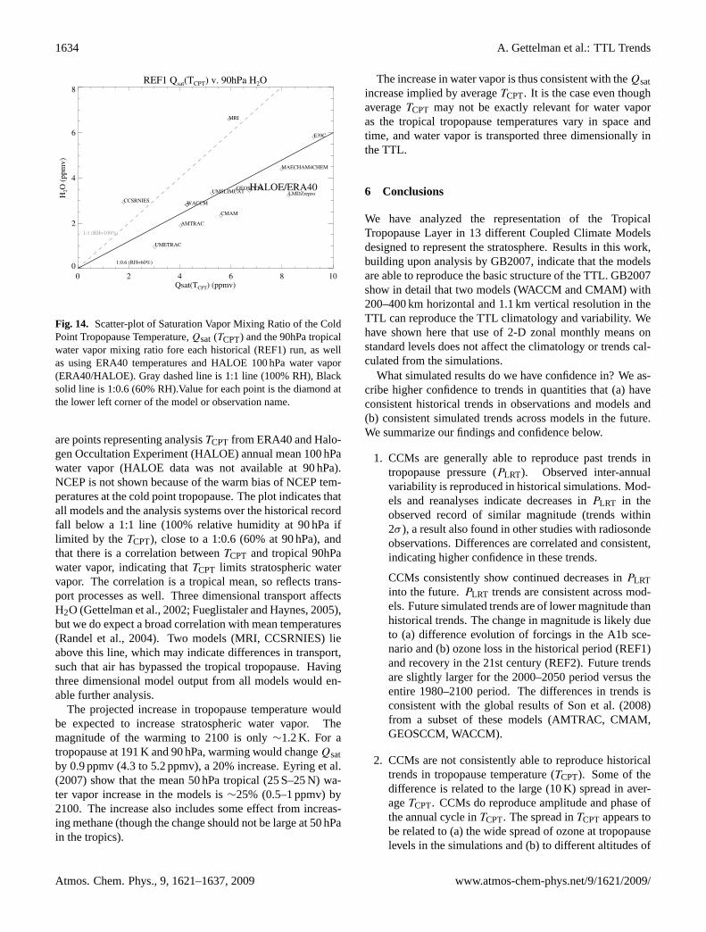
REF1 Qsat(TCPT) v. 90hPa H2O

0 2 4 6 8 10Qsat(TCPT) (ppmv)

0

2

4

6

8

H2O

(ppm

v)

1:1 (RH=100%)

AMTRAC

CCSRNIES

CMAM

E39C

GEOSCCMLMDZrepro

MAECHAM4CHEM

MRI

UMETRAC

UMSLIMCAT

WACCM

HALOE/ERA40

1:0.6 (RH=60%)

Fig. 14. Scatter-plot of Saturation Vapor Mixing Ratio of the Cold Point Tropopause Temperature, Qsat(TCPT )and the 90hPa tropical water vapor mixing ratio fore each historical (REF1) run, as well as using ERA40temperatures and HALOE 100hPa water vapor (ERA40/HALOE). Gray dashed line is 1:1 line (100% RH),Black solid line is 1:0.6 (60% RH).Value for each point is the diamond at the lower left corner of the model orobservation name.

38

Fig. 14. Scatter-plot of Saturation Vapor Mixing Ratio of the ColdPoint Tropopause Temperature,Qsat (TCPT) and the 90hPa tropicalwater vapor mixing ratio fore each historical (REF1) run, as wellas using ERA40 temperatures and HALOE 100 hPa water vapor(ERA40/HALOE). Gray dashed line is 1:1 line (100% RH), Blacksolid line is 1:0.6 (60% RH).Value for each point is the diamond atthe lower left corner of the model or observation name.

are points representing analysisTCPT from ERA40 and Halo-gen Occultation Experiment (HALOE) annual mean 100 hPawater vapor (HALOE data was not available at 90 hPa).NCEP is not shown because of the warm bias of NCEP tem-peratures at the cold point tropopause. The plot indicates thatall models and the analysis systems over the historical recordfall below a 1:1 line (100% relative humidity at 90 hPa iflimited by theTCPT), close to a 1:0.6 (60% at 90 hPa), andthat there is a correlation betweenTCPT and tropical 90hPawater vapor, indicating thatTCPT limits stratospheric watervapor. The correlation is a tropical mean, so reflects trans-port processes as well. Three dimensional transport affectsH2O (Gettelman et al., 2002; Fueglistaler and Haynes, 2005),but we do expect a broad correlation with mean temperatures(Randel et al., 2004). Two models (MRI, CCSRNIES) lieabove this line, which may indicate differences in transport,such that air has bypassed the tropical tropopause. Havingthree dimensional model output from all models would en-able further analysis.

The projected increase in tropopause temperature wouldbe expected to increase stratospheric water vapor. Themagnitude of the warming to 2100 is only∼1.2 K. For atropopause at 191 K and 90 hPa, warming would changeQsatby 0.9 ppmv (4.3 to 5.2 ppmv), a 20% increase.Eyring et al.(2007) show that the mean 50 hPa tropical (25 S–25 N) wa-ter vapor increase in the models is∼25% (0.5–1 ppmv) by2100. The increase also includes some effect from increas-ing methane (though the change should not be large at 50 hPain the tropics).

The increase in water vapor is thus consistent with theQsatincrease implied by averageTCPT. It is the case even thoughaverageTCPT may not be exactly relevant for water vaporas the tropical tropopause temperatures vary in space andtime, and water vapor is transported three dimensionally inthe TTL.

6 Conclusions

We have analyzed the representation of the TropicalTropopause Layer in 13 different Coupled Climate Modelsdesigned to represent the stratosphere. Results in this work,building upon analysis by GB2007, indicate that the modelsare able to reproduce the basic structure of the TTL. GB2007show in detail that two models (WACCM and CMAM) with200–400 km horizontal and 1.1 km vertical resolution in theTTL can reproduce the TTL climatology and variability. Wehave shown here that use of 2-D zonal monthly means onstandard levels does not affect the climatology or trends cal-culated from the simulations.

What simulated results do we have confidence in? We as-cribe higher confidence to trends in quantities that (a) haveconsistent historical trends in observations and models and(b) consistent simulated trends across models in the future.We summarize our findings and confidence below.

1. CCMs are generally able to reproduce past trends intropopause pressure (PLRT). Observed inter-annualvariability is reproduced in historical simulations. Mod-els and reanalyses indicate decreases inPLRT in theobserved record of similar magnitude (trends within2σ ), a result also found in other studies with radiosondeobservations. Differences are correlated and consistent,indicating higher confidence in these trends.

CCMs consistently show continued decreases inPLRTinto the future.PLRT trends are consistent across mod-els. Future simulated trends are of lower magnitude thanhistorical trends. The change in magnitude is likely dueto (a) difference evolution of forcings in the A1b sce-nario and (b) ozone loss in the historical period (REF1)and recovery in the 21st century (REF2). Future trendsare slightly larger for the 2000–2050 period versus theentire 1980–2100 period. The differences in trends isconsistent with the global results ofSon et al.(2008)from a subset of these models (AMTRAC, CMAM,GEOSCCM, WACCM).

2. CCMs are not consistently able to reproduce historicaltrends in tropopause temperature (TCPT). Some of thedifference is related to the large (10 K) spread in aver-ageTCPT. CCMs do reproduce amplitude and phase ofthe annual cycle inTCPT. The spread inTCPT appears tobe related to (a) the wide spread of ozone at tropopauselevels in the simulations and (b) to different altitudes of



the tropopause. Ozone differences are due to both radia-tion and possibly transport. Differences in TCPT are cor-related with differences in simulated stratospheric watervapor.

CCMs show modest and consistent increases in futureTCPT. The “raising and warming” of the tropopause isbroadly consistent with theory. But since raising impliesadiabatic cooling, temperature changes are sensitiveto which of these effects dominates. In these simu-lations, projected tropospheric warming is larger thanstratospheric cooling at the tropopause in the 21st cen-tury. We place only moderate confidence in futureTCPTtrends because of difficulties in reproducing historicaltrends.

3. Over the observed record there are significant changesin the minimum lapse rate level (PLRM). The magnitudeof observed and simulated historical trends is uncertain.The lack of quantitative agreement in historicalPLRMtrends and dependence on convective parameterizationyields lower confidence in future trends.

There are significant and consistent future decreases insimulatedPLRM , amounting to a change of−23 hPaover the 21st century, a significant increase in the meanconvective outflow level of∼250 m. The change is de-pendent on a sub-grid scale process (convection) butis likely driven by surface changes (higher tempera-tures). As a result there is spread to the model trends.Since PLRM decreases faster thanPLRT, simulationsimply a “thinning” of the TTL in the 21st century of−1.7 hPa/decade.

4. TTL anomalies and trends are highly correlatedwith anomalies of near surface tropical temperature.Tropopause pressure and temperature are affected bytropopause level ozone. TTL anomalies are affected lessby stratospheric temperatures. The surface warming ap-pears to be the dominant signal in the TTL across almostall models. The result is consistent across models, indi-cating higher confidence in the conclusion.

5. If tropopause height and particularly temperature trendsare to be believed, it may have significant impacts onstratospheric water vapor due to higher temperatures,with increases in water vapor in the stratosphere pre-dicted. There is consistency between models and obser-vations of the correlation ofTCPT and H2O (though theabsolute value ofTCPT varies).

6. TTL and lower stratospheric ozone anomalies substan-tially influence TTL diagnostics. TTL ozone variestremendously in the simulations, and also seems to becorrelated with the absolute value of tropopause tem-perature. It is critical that models do a better job of sim-ulating TTL ozone.

Acknowledgements.Co-ordination of this study was supportedby the Chemistry-Climate Model Validation Activity (CCMVal)for WCRP’s (World Climate Research Programme) SPARC(Stratospheric Processes and their Role in Climate) project. Thanksto all the CCM groups for their comments on this paper specifically,and generally for their hard work in developing and producingmodel output. We especially thank those model developers who arenot co-authors: J. Austin, T. Nagashima, T. G. Shepherd, S. Paw-son, R. S. Stolarski, M. A. Giorgetta, E. Manzini, M. Deushi,N. Butchart, M. P. Chipperfield and R. R. Garcia. Thanks toK. Rosenlof for discussions. Thanks to the British AtmosphericData Center for assistance with the CCMVal Archive. The NationalCenter for Atmospheric Research is sponsored by the US. NationalScience Foundation. CCSRNIES research was supported by theGlobal Environmental Research Fund (GERF) of the Ministry ofthe Environment (MOE) of Japan (A-071). European CCMValactivities were supported by the European Commission IntegratedProject SCOUT-O3.

Edited by: P. Haynes

References

Akiyoshi, H., Sugita, T., Kanzawa, H., and Kawamoto, N.: Ozoneperturbations in the Arctic summer lower stratosphere as a re-flection of NOx chemistry and planetary scale wave activity, J.Geophys. Res., 109, D03304, doi:10.1029/2003JD003632, 2004.

Austin, J.: A three-dimensional coupled chemistry-climate modelsimulation of past stratospheric trends, J. Atmos. Sci., 59, 218–232, 2002.

Austin, J. and Butchart, N.: Coupled chemistry-climate model sim-ulation for the period 1980 to 2020: ozone depletion and thestart of ozone recovery, Q. J. Roy. Meteor. Soc., 129, 3225–3249,2003.

Austin, J. and Wilson, R. J.: Ensemble simulations of the de-cline and recovery of stratospheric ozone, J. Geophys. Res., 111,D16314, doi:10.1029/2005JD006907, 2006.

Austin, J., Wilson, R. J., Li, F., and Vomel, H.: Evolution of wa-ter vapor concentrations and stratospheric age of air in coupledchemistry-climate model simulations, J. Atmos. Sci., 64, 905–921, 2007.

Beagley, S. R., de Grandpre, J., Koshyk, J., McFarlane, N. A., andShepherd, T. G.: Radiative-dynamical climatology of the first-generation Canadian Middle Atmosphere Model, Atmos. Ocean,35, 293–331, 1997.

Birner, T., Sankey, D., and Shepherd, T. G.: The tropopause in-version layer in models and analyses, Geophys. Res. Lett., 33,L14804, doi:10.1029/2006GL026 549, 2006.

Bloom, S., da Silva, A., Dee, D., Bosilovich, M., Chern, J.-D., Paw-son, S., Schubert, S., Sienkiewicz, M., Stajner, I., Tan, W.-W.,and Wu, M.-L.: Documentation and Validation of the GoddardEarth Observing System (GEOS) Data Assimilation System –Version 4, Tech. Rep. Technical Report Series on Global Model-ing and Data Assimilation 104606, 26, 165 pp., NASA, 2005.

Bony, S., Colman, R., and Kattsov, V. M.: How Well Do We Un-derstand and Evaluate Climate Change Feedback Processes, J.Climate, 19, 3445–3482, 2006.



Butchart, N., Scaife, A. A., Bourqui, M., Grandpre, J., Hare, S.H. E., Kettleborough, J., Langematz, U., Manzini, E., Sassi, F.,Shibata, K., Shindell, D., and Sigmond, M.: Simulations of an-thropogenic change in the strength of the Brewer-Dobson cir-culation, Clim. Dynam., 27, 727–741, doi:10.1007/s00382-006-0162-4, 2006.

Dameris, M., Matthes, S., Deckert, R., Grewe, V., and Ponater, M.:Solar cycle effect delays onset of ozone recovery, Geophys. Res.Lett., 33, L03806, doi:10.1029/2005GL024741, 2006.

Dameris, M., Grewe, V., Ponater, M., Deckert, R., Eyring, V.,Mager, F., Matthes, S., Schnadt, C., Stenke, A., Steil, B., Bruhl,C., and Giorgetta, M. A.: Long-term changes and variability in atransient simulation with a chemistry-climate model employingrealistic forcing, Atmos. Chem. Phys., 5, 2121–2145, 2005,http://www.atmos-chem-phys.net/5/2121/2005/.

de Grandpre, J., Beagley, S. R., Fomichev, V. I., Griffioen, E., Mc-Connell, J. C., Medvedev, A. S., and Shepherd, T. G.: Ozoneclimatology using interactive chemistry: results from the Cana-dian Middle Atmosphere Model, J. Geophys. Res., 105, 26475–26491, 2000.

Efron, B. and Tibshirani, R. J.: An introduction to the Bootstrap,vol. 57 of Monographs on Statistics and Applied Probability,Chapman and Hall, New York, 436 pp., 1993.

Egorova, T., Rozanov, E., Zubov, V., Manzini, E., Schmutz, W.,and Peter, T.: Chemistry-climate model SOCOL: a validation ofthe present-day climatology, Atmos. Chem. Phys., 5, 1557–1576,2005,http://www.atmos-chem-phys.net/5/1557/2005/.

Eyring, V., Butchart, N., and Waugh, D. W.: Assessment of tem-perature, trace species, and ozone in chemistry-climate modelsimulations of the recent past, J. Geophys. Res., 111, D22308,doi:10.1029/2006JD007327, 2006.

Eyring, V., Waugh, D. W., and Bodeker, G. E.: Multi-model projec-tions of stratospheric ozone in the 21st century, J. Geophys. Res.,112, D16303, doi:10.1029/2006JD008332, 2007.

Forster, P. M. d. F. and Shine, K. P.: Assessing the climate impactof trends in stratospheric water vapor, Geophys. Res. Lett., 29,1086, doi:10.1029/2001GL013909, 2002.

Fueglistaler, S. and Haynes, P. H.: Control of interannual andlonger-term variability of stratospheric water vapor, J. Geophys.Res., 110, D24108, doi:10.1029/2005JD006019, 2005.

Garcia, R. R., Marsh, D. R., Kinnison, D. E., Boville, B.A., and Sassi, F.: Simulation of secular trends in the mid-dle atmosphere, 1950–2003, J. Geophys. Res., 112, D09301,doi:10.1029/2006JD007485, 2007.

Gettelman, A. and Birner, T.: Insights on Tropical TropopauseLayer Processes using Global Models, J. Geophys. Res., 112,D23104, doi:10.1029/2007JD008945, 2007.

Gettelman, A. and Forster, P. M. F.: A Climatology of the TropicalTropopause Layer, J. Met. Soc. Jpn., 80, 911–924, 2002.

Gettelman, A. and Kinnison, D. E.: The global impact of super-saturation in a coupled chemistry-climate model, Atmos. Chem.Phys., 7, 1629–1643, 2007,http://www.atmos-chem-phys.net/7/1629/2007/.

Gettelman, A., Randel, W. J., Massie, S., Wu, F., Read, W. G., andRussell III, J. M.: El-Nino as a natural experiment for studyingthe tropical tropopause region, J. Climate, 14, 3375–3392, 2001.

Gettelman, A., Randel, W. J., Wu, F., and Massie, S. T.: Transportof water vapor in the tropical tropopause layer, Geophys. Res.Lett., 29, 1009, doi:10.1029/2001GL013818, 2002.

Holton, J. R. and Gettelman, A.: Horizontal transport and dehy-dration in the stratosphere, Geophys. Res. Lett., 28, 2799–2802,2001.

IPCC: Special Report on Emission Scenarios, Cambridge Univer-sity Press, New York, 612 pp., 2000.

Johns, T. C., Durman, C. F., and Banks, H. T.: The new HadleyCentre climate model Had-GEM1: Evaluation of coupled simu-lations, J. Climate, 19, 1327–1353, 2006.

Jourdain, L., Bekki, S., Lott, F., and Lefevre, F.: The coupledchemistry-climate model LMDz-REPROBUS: description andevaluation of a transient simulation of the period 1980–1999,Ann. Geophys., 26, 1391–1413, 2008,http://www.ann-geophys.net/26/1391/2008/.

Kalnay, E., Kanamitsu, M., Kistler, R., Collins, W., Deaven, D.,Gandin, L., Iredell, M., Saha, S., White, C., Woollen, J., Zhu,Y., Chelliah, M., Ebisuzaki, W., Higgins, W., Janowiak, J., Mo,K. C., Ropelewski, C., Wang, J., Leetmaa, A., Reynolds, R.,Jenne, P., and Joseph, D.: The NCEP/NCAR 40-year reanaly-sis project, B. Am. Meteorol. Soc., 77, 437–471, 1996.

Kurokawa, J., Akiyoshi, H., Nagashima, T., Masunaga, H.,Nakajima, T., Takahashi, M., and Nakane, H.: Effects ofatmospheric sphericity on stratospheric chemistry and dy-namics over Antarctica, J. Geophys. Res., 110, D21305,doi:10.1029/2005JD005798, 2005.

Lott, F. L., Hourdin, F., and Levan, P.: The stratospheric ver-sion of LMDz: Dynamical Climatologies, Arctic Oscillation andImpact on the Surface Climate, Clim. Dynam., 25, 851–868,doi:10.1007/s00382-005-0064-x, 2005.

Manzini, E., Steil, B., Bruhl, C., Giorgetta, M. A., and Kruger,K.: A new interactive chemistry climate model. 2: Sensitivityof the middle atmosphere to ozone depletion and increase ingreenhouse gases: implications for recent stratospheric cooling,J. Geophys. Res., 108(D14), 4429, doi:10.1029/2002JD002977,2003.

Meehl, G. A., Washington, W. M., Santer, B. D., Collins, W. D.,Arblaster, J. M., Hu, A., Lawrence, D. M., Teng, H., Buja, L. E.,and Strand, W. G.: Climate Change Projections for the Twenty-First Century and Climate Change Commitment in CCSM3, J.Climate, 19, 2597–2616, 2006.

Pawson, S. and Fiorino, M.: A comparison of reanalyses in the trop-ical stratosphere, Part 3, Inclusion of the pre-satellite data era,Clim. Dynam., 15, 241–250, 1999.

Pitari, G., Mancini, E., Rizzi, V., and Shindell, D.: Impact of fu-ture climate and emission changes on stratospheric aerosols andozone, J. Atmos. Sci., 59, 414–440, 2002.

Randel, W. J., Wu, F., Oltmans, S. J., Rosenlof, K., and Nedoluha,G. E.: Interannual changes of stratospheric water vapor and cor-rellations with tropical tropopause temperatures, J. Atmos. Sci.,61, 2133–2148, 2004.

Randel, W. J., Wu, F., Vomel, H., Nedoluha, G. E., andForster, P. F.: Decreases in stratospheric water vapor since2001: links to changes in the tropical tropopause and theBrewer-Dobson Circulation, J. Geophys. Res., 111, D12312,doi:10.1029/2005JD006744, 2006.

Rozanov, E., Schraner, M., Schnadt, C., Egorova, T., Wild, M.,Ohmura, A., Zubov, V., Schmutz, W., and Peter, T.: Assess-ment of the ozone and temperature variability during 1979–1993with the chemistry-climate model SOCOL, Adv. Space. Res., 35,1375–1384, 2005.


http://www.atmos-chem-phys.net/5/2121/2005/



http://www.ann-geophys.net/26/1391/2008/


Santer, B. D., Wehner, M. F., Wigley, T. M. L., Sausen, R., Meehl,G. A., Taylor, K. E., Ammann, C., Arblaster, J., Washington,W. M., Boyle, J. S., and Bruggemann, W.: Contributions of An-thropogenic and Natural Forcing to Recent Tropopause HeightChanges, Science, 301, 479–483, doi:10.1126/science.1084123,2003.

Santer, B. D., Wigley, T. M. L., and Mears, C.: Am-plification of Surface Temperature Trends and Variabil-ity in the Tropical Atmosphere, Science, 309, 1551–1556,doi:10.1126/science.1114867, 2005.

Seidel, D. J. and Randel, W. J.: Variability and trends in the globaltropopause estimated from Radiosonde data, J. Geophys. Res.,111, D21101, doi:10.1029/2006JD007363, 2006.

Seidel, D. J., Ross, R. J., Angell, J. K., and Reid, G. C.: Climato-logical characteristics of the tropical tropopause as revealed byRadiosondes, J. Geophys. Res., 106, 7857–7878, 2001.

Seidel, D. J., Fu, Q., Randel, W. J., and Reichler, T.: Widening ofthe tropical belt in a changing climate, Naure Geosci., 1, 21–24,doi:10.1038/ngeo.2007.38, 2008.

Shibata, K. and Deushi, M.: Partitioning between resolved waveforcing and unresolved gravity wave forcing to the quasi-biennialoscillation as revealed with a coupled chemistry-climate model,Geophys. Res. Lett., 32, L12820, doi:10.1029/2005GL022885,2005.

Shibata, K., Deushi, M., Sekiyama, T. T., and Yoshimura, H.: De-velopment of an MRI chemical transport model for the study ofstratospheric chemistry, Papers in Met. and Geophys., 55, 75–119, 2005.

Solomon, S., Qin, D., Manning, M., Chen, Z., Marquis, M., Averyt,K. B., Tignor, M., and Miller, H. L.: Climate Change 2007 – ThePhysical Science Basis: Working Group I Contribution to theFourth Assessment Report of the IPCC (Climate Change 2007),Cambridge University Press, Cambridge, UK, 1008 pp., 2007.

Son, S. W., Polvani, L. M., Waugh, D. W., Birner, T., Akiyoshi, H.,Garcia, R. R., Gettelman, A., Plummer, D. A., and Rozanov, E.:The impact of stratospheric ozone recovery on tropopause heighttrends, J. Climate, 2008.

Steil, B., Bruhl, C., Manzini, E., Crutzen, P. J., Lelieveld, J., Rasch,P. J., Roeckner, E., and Kruger, K.: A new interactive chem-istry climate model. 1: Present day climatology and interan-nual variability of the middle atmosphere using the model and9 years of HALOE/UARS data, J. Geophys. Res., 108, 4290,doi:10.1029/2002JD002971, 2003.

Stephens, G. L.: Cloud Feedbacks in the Climate System: A CriticalReview, J. Climate, 18, 237–273, 2005.

Stolarski, R. S., Douglass, A. R., Steenrod, S., and Pawson, S.:Trends in Stratospheric Ozone: Lessons Learned from a 3DChemical Transport Model, J. Atmos. Sci., 63, 1028–1041, 2006.

Struthers, H., Kreher, K., Austin, J., Schofield, R., Bodeker, G.,Johnston, P., Shiona, H., and Thomas, A.: Past and future simu-lations of NO2 from a coupled chemistry-climate model in com-parison with observations, Atmos. Chem. Phys., 4, 2227–2239,2004,http://www.atmos-chem-phys.net/4/2227/2004/.

Thuburn, J. and Craig, G. C.: On the temperature structureof the tropical substratosphere, J. Geophys. Res., 107, 4017,doi:10.1029/2001JD000448, 2002.

Tian, W. and Chipperfield, M. P.: A new coupled chemistryclimatemodel for the stratosphere: The importance of coupling for futureO3-climate predictions, Q. J. Roy. Meteor. Soc., 131, 281–304,2005.

Uppala, S., Kallberg, P., Simmons, A., Andrae, U., da Costa Bech-told, V., Fiorino, M., Gibson, J., Haseler, J., Hernandez, A.,Kelly, G., Li, X., Onogi, K., Saarinen, S., Sokka, N., Allan, R.,Andersson, E., Arpe, K., Balmaseda, M., Beljaars, A., van deBerg, L., Bidlot, J., Bormann, N., Caires, S., Chevallier, F., De-thof, A., Dragosavac, M., Fisher, M., Fuentes, M., Hagemann,S., Holm, E., Hoskins, B., Isaksen, L., Janssen, P., Jenne, R., Mc-Nally, A., Mahfouf, J.-F., Morcrette, J.-J., Rayner, N., Saunders,R., Simon, P., Sterl, A., Trenberth, K., Untch, A., Vasiljevic, D.,Viterbo, P., and Woollen, J.: The ERA-40 re-analysis, Q. J. Roy.Meteor. Soc., 131, 2961–3012, 2005.

WMO (World Meteorological Organization), Scientific Assessmentof Ozone Depletion: 2002, Global Ozone Research and Moni-toring Project – Report No. 47, 498 pp., Geneva, Switzerland,2003.

WMO (World Meteorological Organization), Scientific Assessmentof Ozone Depletion: 2006, Global Ozone Research and Moni-toring Project – Report No. 50, 572 pp., Geneva, Switzerland,2007.

Yin, J. H.: A consistent poleward shift of the storm tracks in simu-lations of 21st century climate, Geophys. Res. Lett., 32, L18701,doi:10.1029/2005GL023684, 2005.



the tropical tropopause layer 1960–2100 · the tropical tropopause layer 1960–2100 a....

Documents