the sufficient statistic approach: predicting the … · the sufficient statistic approach:...
TRANSCRIPT
Research Division Federal Reserve Bank of St. Louis Working Paper Series
The Sufficient Statistic Approach: Predicting the Top of the Laffer Curve
Alejandro Badel and
Mark Huggett
Working Paper 2015-038A http://research.stlouisfed.org/wp/2015/2015-038.pdf
November 2015
FEDERAL RESERVE BANK OF ST. LOUIS Research Division
P.O. Box 442 St. Louis, MO 63166
______________________________________________________________________________________
The views expressed are those of the individual authors and do not necessarily reflect official positions of the Federal Reserve Bank of St. Louis, the Federal Reserve System, or the Board of Governors.
Federal Reserve Bank of St. Louis Working Papers are preliminary materials circulated to stimulate discussion and critical comment. References in publications to Federal Reserve Bank of St. Louis Working Papers (other than an acknowledgment that the writer has had access to unpublished material) should be cleared with the author or authors.
The Sufficient Statistic Approach:Predicting the Top of the Laffer Curve∗
Alejandro BadelFederal Reserve Bank of St. [email protected]
Mark HuggettGeorgetown [email protected]
this draft: November 10, 2015
Abstract
We provide a formula for the tax rate at the top of the Laffer curve as a function of three elastic-ities. Our formula applies to static models and to steady states of dynamic models. One of theelasticities that enters our formula has been estimated in the elasticity of taxable income litera-ture. We apply standard empirical methods from this literature to data produced by reformingthe tax system in a model economy. We find that these standard methods underestimate therelevant elasticity in models with endogenous human capital accumulation.
Keywords: Sufficient Statistic, Laffer Curve, Marginal Tax Rate, Elasticity
JEL Classification: D91, E21, H2, J24
∗This work used the Extreme Science and Engineering Discovery Environment (XSEDE) Grant SES 130025,supported by the National Science Foundation, to access the Stampede cluster at the Texas Advanced Com-puting Center. This work also used the cluster at the Federal Reserve Bank of Kansas City.
1 Introduction
Imagine that an important public policy issue, involving the functioning of the entire economy,
could be settled by a simple formula together with only a few inputs estimated from data.
Imagine further that the simple formula, connecting the public policy variable to empirical
inputs, was general in that it held within a wide class of theoretical models that were rele-
vant to the issue at hand. The scenario just described is the goal of the sufficient statistic
approach. Chetty (2009) states “The central concept of the sufficient statistic approach ... is to
derive formulas for the welfare [revenue] consequences of policies that are functions of high-level
elasticities rather than deep primitives.”
An important application of the sufficient statistic approach is to predict the tax rate at the
top of the Laffer curve (i.e. the revenue maximizing tax rate). Thus, the public policy variable
under consideration is a tax rate on some specified component of income or expenditure. This
could be the tax rate on consumption, labor income, capital income or something more specific
such as the top federal tax rate on ordinary income.
One may want to predict the top of the Laffer curve for several reasons. First, it may be
widely agreed that setting a tax rate beyond the revenue maximizing rate is counterproductive.
If so, an accurate prediction usefully narrows the tax policy debate. Second, one may argue,
following Diamond and Saez (2011), that the revenue maximizing tax rate on top earners
closely approximates the welfare maximizing top tax rate for some welfare criteria. From this
perspective, the revenue maximizing tax rate then becomes a quantitative policy guide.
From a quick look at the literature, one might conclude that the theoretical groundwork on
this issue is complete. There is a widely-used sufficient statistic formula τ ∗ = 1/(1 + aε) that
characterizes the revenue maximizing marginal tax rate τ ∗ that applies beyond a threshold.
Moreover, there is also a closely related formula τ ∗ = (1 − g)/(1 − g + aε) for the welfare
maximizing marginal tax rate that is stated in terms of the same two empirical inputs (a, ε)
and a social welfare weight g ≥ 0 put on the marginal consumption of top earners. See Diamond
and Saez (2011), Piketty and Saez (2013) among many others for a discussion of these formulae.
The Mirrlees Review uses them to offer quantitative advice for setting the top income tax rate
- see Adam et al. (2010, Chapter 2).
A more critical reading of the literature suggests that the widely-used formula does not actually
apply to a wide class of relevant models. The widely-used formula τ ∗ = 1/(1 + aε) is not valid
in dynamic models. For example, it does not apply to steady states in either the infinitely-lived
agent or the overlapping generations versions of the neoclassical growth model. These are the
two workhorse models of modern macroeconomics. A large literature analyzes the taxation of
2
consumption, labor income and capital income using these models.1 The widely-used formula
does not apply to the class of heterogeneous-agent models that currently dominate as positive
models of the distribution of earnings, income, consumption and wealth.2
The sufficient-statistic formula in Theorem 1 of this paper applies to static models and to steady
states of dynamic models. Specifically, we show that it applies to the Mirrlees (1971) model, to
the two workhorse models of modern macroeconomics and to human capital models. Theorem
1 is stated in terms of three elasticities including the single elasticity of the widely-used formula.
One of the new elasticities captures the possibility, within dynamic models, that revenue from
agent types below the threshold will respond to changes in the top rate. For example, this
can occur because such agents anticipate the possibility of passing the threshold later in life.
The other new elasticity captures the possibility that agent types that are above the threshold
have incomes or expenditures that are taxed separately. For example, consumption and various
types of capital income are commonly taxed separately from labor income. The formula in
Theorem 1 allows both of these new elasticities to be non-zero.
This paper makes two contributions. First, Theorem 1 provides a tax rate formula with wide
application yet it is stated in terms of only three elasticities. Thus, the formula in Theorem 1
should replace the widely-used formula in future work. It should also help guide future empirical
work that estimates elasticities. Currently, there are no estimates in the literature for two of
the three elasticities that enter the formula. Second, we bench test the formula using a human
capital model. One message from the bench test is that the formula accurately predicts the top
of the Laffer curve even when the top tax rate in the model is initially quite far from the revenue
maximizing top tax rate. This is important because prediction is precisely the intended use of
the formula in applied work. A second message of the bench test is that standard methods, from
the elasticity of taxable income literature, underestimate one key elasticity in the human capital
model. An underestimated elasticity would lead one to overstate the revenue maximizing top
tax rate. Future work should develop methods to accurately estimate the three key long-run
elasticities in different modeling frameworks and then apply these methods to data.
Our paper is most closely related to three literatures. First, it relates to the optimal labor
income taxation literature. See Piketty and Saez (2013) for a review that highlights sufficient
statistic formulae. Second, it relates to the class of heterogeneous-agent models surveyed by
1Auerbach and Kotlikoff (1987) is an early quantitative exploration of tax reforms within overlapping gen-erations models.
2Heathcote, Storesletten and Violante (2009) review this literature. The models that they review featureagents that are ex-ante heterogeneous, face idiosyncratic risk and trade in incomplete financial markets. Badeland Huggett (2014), Guner, Lopez-Daneri and Ventura (2014) and Kindermann and Krueger (2014) computeLaffer curves produced by changing top tax rates within such models and examine the resulting steady states.Altig and Carlstrom (1999) analyze implications of changing tax progressivity in a model without idiosyncraticrisk.
3
Heathcote, Storesletten and Violante (2009) because our tax rate formula applies to many
models in this large class. Badel and Huggett (2014) apply our tax rate formula to a specific
heterogeneous-agent model and find it accurately predicts the top of the model Laffer curve.
Our formula could also be applied to the models in Guner, Lopez-Daneri and Ventura (2014)
and Kindermann and Krueger (2014) to better understand why these quantitative models have
substantially different revenue maximizing top tax rates. Third, it relates to the elasticity of
taxable income literature - a key source of elasticity estimates for sufficient statistic formulae.
Saez, Slemrod and Giertz (2012) survey this literature. The work of Golosov, Tsyvinski and
Werquin (2014) is close in some respects to our work. They analyze local perturbations of tax
systems of a more general type than the elementary perturbation that we analyze. Our formula
applies to a much wider class of models.
The paper is organized as follows. Section 2 presents the tax rate formula. Section 3 shows
that the formula applies in a straightforward way to several classic static and dynamic mod-
els. Section 4 bench tests the formula using a quantitative human capital model. Section 5
concludes.
2 Tax Rate Formula
The tax rate formula is based on three basic model elements: (i) a distribution of agent types
(X,X ,P), (ii) an income choice y(x, τ) that maps an agent type x ∈ X and a parameter τ
of the tax system into an income choice and (iii) a class of tax functions T (y; τ) mapping
income choice and a tax system parameter τ into the total tax paid. Total tax revenue is then∫XT (y(x, τ); τ)dP . Our approach does not rely on specifying an explicit dynamic or static
equilibrium model up front. Instead, our tax rate formula can be applied in a straightforward
way by mapping equilibrium allocations of specific static or dynamic models into these three
basic model elements.
2.1 Assumptions
Assumption A1 says that the distribution of agent types is represented by a probability space
composed of a space of types X, a σ-field X on X and a probability measure P defined over
sets in X . Assumption A2 places structure on the class of tax functions. The tax functions
differ in a single parameter τ , where τ is interpreted as the linear tax rate that applies to
income beyond a threshold y. Below this threshold the tax function can be nonlinear but
all tax functions in the class are the same below the threshold. Assumption A3 says that
key aggregates are differentiable in τ . The aggregates are based on integrals over the sets
4
X1 = {x ∈ X : y(x, τ ∗) > y} and X2 = X − X1 in X , where τ ∗ ∈ (0, 1) is a fixed value that
serves to define and fix these sets.
A1. (X,X ,P) is a probability space.
A2. There is a threshold y ≥ 0 such that
(i) T (y; τ)− T (y; τ) = τ [y − y], ∀y > y,∀τ ∈ (0, 1) and
(ii) T (y; τ) = T (y; τ ′),∀y ≤ y,∀τ, τ ′ ∈ (0, 1).
A3.∫X1y(x, τ)dP and
∫X2T (y(x, τ); τ)dP are strictly positive and are differentiable in τ .
We also consider a generalization where the tax system depends on n ≥ 2 components of income
or expenditure. The three basic elements of the generalized model are (i) a distribution of agent
types (X,X ,P), (ii) an n ≥ 2 dimensional income-expenditure choice (y1(x, τ), ..., yn(x, τ)) and
(iii) a class of tax functions T (y1, ..., yn; τ) mapping the vector of choices and a tax system
parameter τ into the total tax paid.
Assumptions A1′ − A3′ restate assumptions A1 - A3 for the generalized model. A2′ assumes
that the tax system is additively separable in that the first component of income y1 determines
a portion of the tax liability of an agent separately from the other components. For example,
this structure captures a situation where labor income y1 and capital income y2 are taxed using
separate tax schedules or where labor income y1 and consumption y2 are taxed separately.
Alternatively, one might view y1 as being ordinary income and y2 as being the sum of long-
term capital gains and qualified dividends as defined by the Internal Revenue Service in the
US. In Assumption A3′ the integrals are calculated over the sets X1 = {x ∈ X : y1(x, τ ∗) > y}and X2 = X −X1, where τ ∗ ∈ (0, 1) is a fixed value.
A1′. (X,X ,P) is a probability space.
A2′. T is separable in that T (y1, ..., yn; τ) = T1(y1; τ) + T2(y2, ..., yn),∀(y1, ..., yn, τ). Moreover,
there is a threshold y ≥ 0 such that
(i) T1(y1; τ)− T1(y; τ) = τ [y1 − y],∀y1 > y,∀τ ∈ (0, 1) and
(ii) T1(y1; τ) = T1(y1; τ ′), ∀y1 ≤ y,∀τ, τ ′ ∈ (0, 1).
A3′.∫X1y1dP,
∫X1T2(y2, ..., yn)dP and
∫X2T (y1, ..., yn; τ)dP are strictly positive and are differ-
entiable in τ .
5

2.2 Formula
Before stating the formula in Theorem 1, we express total tax revenue as the sum of tax revenue
from the set of agent types with incomes above a threshold X1 = {x ∈ X : y(x, τ ∗) > y} and
from all remaining types X2 = X −X1. Total tax revenue can be stated in the same manner
when the tax system depends on n ≥ 2 components of income or expenditure by again defining
two sets X1 = {x ∈ X : y1(x, τ ∗) > y} and X2 = X −X1. This is done below.
∫XT (y(x, τ); τ)dP =
∫X1T (y(x, τ); τ)dP +
∫X2T (y(x, τ); τ)dP
∫XT (y1, ..., yn; τ)dP =
∫X1T (y1, ..., yn; τ)dP +
∫X2T (y1, ..., yn; τ)dP
With these expressions in hand, we now state the theorem.
Theorem 1:
(i) Assume A1− A3. If τ ∗ ∈ (0, 1) is revenue maximizing, then τ ∗ = 1−a2ε21+a1ε1
, where
(a1, a2) = (
∫X1ydP∫
X1
[y − y
]dP
,
∫X2T (y; τ ∗)dP∫
X1
[y − y
]dP
) and (ε1, ε2) = (d log
∫X1ydP
d log(1− τ),d log
∫X2T (y; τ ∗)dP
d log(1− τ)).
(ii) Assume A1′ − A3′. If τ ∗ ∈ (0, 1) is revenue maximizing, then τ ∗ = 1−a2ε2−a3ε31+a1ε1
, where
(a1, a2, a3) = (
∫X1y1dP∫
X1
[y1 − y
]dP
,
∫X2T (y1, ..., yn; τ ∗)dP∫X1
[y1 − y
]dP
,
∫X1T2(y2, ..., yn)dP∫X1
[y1 − y
]dP
) and
(ε1, ε2, ε3) = (d log
∫X1y1dP
d log(1− τ),d log
∫X2T (y1, ..., yn; τ ∗)dP
d log(1− τ),d log
∫X1T2(y2, ..., yn)dP
d log(1− τ)).
Proof:
(i) If τ ∗ ∈ (0, 1) maximizes revenue then it also maximizes τ∫X1
[y(x; τ)−y]dP+∫X2T (y(x; τ), τ)dP .
This holds by subtracting the constant term∫X1T (y; τ)dP from total revenue and using A2.
The following necessary condition then holds:
6

∫X1
[y(x, τ ∗)− y
]dP − τ ∗
d∫X1y(x; τ ∗)dP
d(1− τ)−d∫X2T (y(x, τ ∗); τ ∗)dP
d(1− τ)= 0
Divide the necessary condition by∫X1
[y(x, τ ∗)− y
]dP and rearrange using the elasticities
stated in the Theorem. This implies 1 − τ∗
1−τ∗a1ε1 − 11−τ∗a2ε2 = 0 which in turn implies
τ ∗ = 1−a2ε21+a1ε1
.
(ii) If τ ∗ ∈ (0, 1) maximizes revenue then it also maximizes τ∫X1
(y1−y)dP+∫X1T2(y2, ..., yn)dP+∫
X2T (y1, ..., yn; τ)dP . This holds by subtracting the constant term
∫X1T1(y; τ)dP from total
revenue and using A2’. The following necessary condition then holds:
∫X1
[y1 − y
]dP − τ ∗
d∫X1y1dP
d(1− τ)−d∫X1T2(y2, ..., yn)dP
d(1− τ)−d∫X2T (y1, ..., yn; τ ∗)dP
d(1− τ)= 0
Divide all terms in the previous equation by∫X1
[y1 − y
]dP and then rearrange using the
elasticities stated in the Theorem. This implies 1− τ∗
1−τ∗a1ε1 − 11−τ∗a2ε2 − 1
1−τ∗a3ε3 = 0 which
in turn implies τ ∗ = 1−a2ε2−a3ε31+a1ε1
. ‖
Comments:
1. The formula is appealing from the perspective of the sufficient statistic approach. It is stated
in terms of at most three elasticities. Nevertheless, it applies to economies where taxes are
determined based on many different income or expenditure types. It applies to non-parametric
economic models analyzed in partial or in general equilibrium. Thus, it does not require
assumptions on functional forms for the primitives of specific models. However, it does require
that certain aggregates are differentiable in the tax parameter.
2. The widely-used formula τ ∗ = 1/(1 +aε) is effectively a special case of the sufficient statistic
formula in Theorem 1. What type of situations does the widely-used formula not address
that the formula in Theorem 1 successfully addresses? There are two general categories. The
first category includes situations where agent types below the threshold, in the set X2, have
their income and expenditures (y1, ..., yn) and corresponding tax liabilities change as τ changes.
This can happen, in static or dynamic models, when factor prices change due to the response
from agent types above the threshold. In dynamic models this can also happen because agents
transit through the income distribution. Thus, agents can be below the threshold at one age
7
and above it at a later age. This implies that “agent types” below the threshold can have
income or expenditure choices that vary with τ . In all these circumstances the tax revenue
from agent types in X2 changes as τ changes and thus the term a2ε2 is non-zero.
The second category covers scenarios in which many components of income or expenditure are
taxed in practice. Consider a change in the parameter τ that governs the taxation of component
y1. Then agent types above the threshold, in the set X1, will adjust other components (y2, ..., yn)
of income or expenditure. The revenue consequences of such adjustments need to be accounted
for. The term a3ε3 will be non-zero when these revenues change. The next two sections give
concrete examples of when the terms a2ε2 or a3ε3 are non-zero.
3. To state the formula using elasticities requires that each of the integrals (e.g.∫X2T (y; τ)dP ),
over which the elasticity is taken, is non-zero. If any of the integral terms is zero, then the
result can still be stated but without using an elasticity for that integral. For example, if the
integral∫X2T (y; τ)dP is zero (i.e. total net taxes on agent types below the threshold are zero)
and the integral does not vary on the margin as the tax rate τ varies, then the term a2ε2 in
the formula in Theorem 1 can be replaced with a zero. Examples 1 and 3 in the next section
illustrate this point.
3 Examples
We now consider three classic models: the Mirrlees model as well as the overlapping genera-
tions and infinitely-lived agent versions of the neoclassical growth model. We map equilibrium
elements in each model into the language of Theorem 1. While the examples associate the tax
rate parameter τ with a labor income tax rate, this is purely for convenience.
3.1 Example 1: Mirrlees Model
Mirrlees (1971) considered a static model in which agents make a consumption and labor deci-
sion in the presence of a tax and transfer system. In our version of this model, the government
runs a balanced budget where taxes fund a lump-sum transfer Tr(τ). The model’s primitives
are a utility function u(c, l), agent’s productivity x ∈ X, a productivity distribution P and a
class of tax functions T (y; τ).
Definition: An equilibrium is (c(x; τ), l(x; τ), T r(τ)) such that given any τ ∈ (0, 1)
1. optimization: (c(x; τ), l(x; τ)) ∈ argmax{u(c, l) : (1 + τc)c ≤ wxl(1− τ) + Tr(τ), l ≥ 0}
2. market clearing:∫Xc(x; τ)dP = w
∫Xxl(x; τ)dP
8

3. government budget: Tr(τ) = τ∫Xwxl(x; τ)dP + τc
∫Xc(x; τ)dP
We state equilibria in closed form using the following functional forms and restrictions:
u(c, l) = c− α l1+1ν
1+ 1ν
and α, ν > 0
X = R+ and (X,X , P ) implies that∫Xx1+νdP is finite and P (0) = 0
Equilibrium allocations are straightforward to state:
l(x; τ) = [wx(1−τ)α(1+τc)
]ν
c(x; τ) = [wx[wx(1−τ)α(1+τc)
]ν(1− τ) + Tr(τ)]/(1 + τc)
Tr(τ) = (τ + τc)w1+ν [ (1−τ)
α(1+τc)]ν∫Xx1+νdP
We now map equilibrium allocations into the elements used to state Theorem 1.
Step 1: Set (X,X , P ) to the probability space used in Example 1.
Step 2: Set y1(x, τ) = wxl(x; τ) and y2(x, τ) = c(x; τ)
Step 3: Set T (y1, y2; τ) = τy1 + τcy2.
We now calculate the terms in the formula. It is clear that a1 = 1 as the threshold is y = 0 and
that ε1 = ν by a direct calculation of the elasticity.3 It is also clear that∫X2T (y1, y2; τ)dP = 0
as effectively all agent types are above the threshold as P (X2) = P (0) = 0. Thus, the term
a2ε2 in the formula can be replaced with a zero, consistent with Comment 3 to Theorem 1. It
is easy to see that (a3, ε3) = (τc, ν). Finally, it is also easy to calculate the revenue maximizing
tax rate directly and see that it agrees with the rate implied by the formula.
τ ∗ =1− a2ε2 − a3ε3
1 + a1ε1=
1− 0− τcν1 + 1× ν
=1− τcν1 + ν
3Theorem 1 directs one to calculate the elasticities and the related coefficients when the sets (X1, X2) aredefined at the revenue maximizing tax rate τ∗. We calculate (a1, ε1) = (1, ν) when these sets are specified forany fixed value of τ ∈ (0, 1).
9
3.2 Example 2: Diamond Growth Model
Diamond (1965) analyzes an overlapping generations model with two-period lived agents and
a neoclassical production function F (K,L) with constant returns. In the model, age 1 and
age 2 agents are equally numerous at any point in time and each age group has a mass of
1. Agents solve problem P1, where they choose labor, consumption and savings when young.
They face proportional labor income and consumption taxes with rates τ and τc, respectively.
The government collects taxes and makes a lump-sum transfer Tr(τ) to young agents.
(P1) maxU(c1, c2, l) s.t.
(1 + τc)c1 + k ≤ w(τ)zl(1− τ) + Tr(τ), (1 + τc)c2 ≤ k(1 + r(τ)) and l ∈ [0, 1]
Age 1 agents are heterogeneous in labor productivity z ∈ Z ⊂ R+. The distribution of labor pro-
ductivity is given by a probability space (Z,Z, P ). Define two aggregates K(τ) =∫Zk(z; τ)dP
and L(τ) =∫Zzl(z; τ)dP .
Definition: A steady-state equilibrium is (c1(z; τ), c2(z; τ), l(z; τ), k(z; τ)), a transfer Tr(τ)
and factor prices (w(τ), r(τ)) such that for any τ ∈ (0, 1)
1. optimization: (c1(z; τ), c2(z; τ), l(z; τ), k(z; τ)) solve P1.
2. factor prices: w(τ) = F2(K(τ), L(τ)) and 1 + r(τ) = F1(K(τ), L(τ))
3. market clearing:∫Z
(c1(z; τ) + c2(z; τ))dP +K(τ) = F (K(τ), L(τ))
4. government budget: Tr(τ) = τc∫Z
(c1(z; τ) + c2(z; τ))dP + τ∫Zw(τ)zl(z; τ)dP
We now map equilibrium allocations into the language used to state Theorem 1.
Step 1: Define the probability space of agent types. An agent type is x = (z, j) consisting of
the agent’s productivity z when young and the agent’s current age j.
x = (z, j) ∈ X = Z × {1, 2} and P (A) =
∫Z
[1
21{(z,1)∈A} +
1
21{(z,2)∈A}]dP ,∀A ∈ X
Step 2: Define choices (y1, y2) as labor income and consumption, respectively.
(y1(x; τ), y2(x; τ)) =
(w(τ)zl(z; τ), c1(z; τ)) for x = (z, 1),∀z ∈ Z
(0, c2(z; τ)) for x = (z, 2),∀z ∈ Z
10
Step 3: Set T (y1, y2; τ) = τy1 + τcy2. Aggregate taxes∫XT (y1, y2; τ)dP are proportional to
the right-hand side of equilibrium condition 4.
The coefficients premultiplying each of the elasticities are easy to determine. The threshold
is y = 0 as the tax τ is a proportional labor income tax. The coefficients are (a1, a2, a3) =
(1,τc
∫Z c2(z;τ∗)dP
w(τ∗)L(τ∗),τc
∫Z c1(z;τ∗)dP
w(τ∗)L(τ∗)). The coefficient a2 from Theorem 1 is the ratio of the total tax
revenue from agent types in X2 to the total incomes y1 above the threshold y for agent types
in X1. This equals the ratio of total consumption taxes paid by age 2 agents to total labor
income. The coefficient a3 is the ratio of total tax revenue from agents in X1 on types of income
or expenditure other than type y1 to total incomes y1 above the threshold.
τ ∗ =1− a2ε2 − a3ε3
1 + a1ε1
=1− τc
∫Z c2(z;τ∗)dP
w(τ∗)L(τ∗)× ε2 −
τc∫Z c1(z;τ∗)dP
w(τ∗)L(τ∗)× ε3
1 + 1× ε1
The take-away point from Example 2 is that the formula in Theorem 1 applies to steady states
of dynamic models once an agent type is viewed in the right way.4
3.3 Example 3: Trabandt and Uhlig
Trabandt and Uhlig (2011) analyze Laffer curves using the neoclassical growth model. The
model features a production function F (k, l) and an infinitely-lived agent. They calibrate
some model parameters so that steady states of their model match aggregate features of the
US economy and 14 European economies and preset other model parameters. They calculate
Laffer curves by varying either the tax rate on labor income, capital income or consumption to
determine how the steady-state equilibrium lump-sum transfer responds to the tax rate. We
show that our sufficient statistic formula applies to Laffer curves in their model. We focus on
the Laffer curve related to varying the labor income tax rate, but our formula also applies to
the Laffer curves arising from varying the other tax rates in their model.
The equilibrium concept given below differs from that in Trabandt and Uhlig in that it abstracts
from steady-state growth and imports in order to simplify the exposition.
(P1) max∑∞
t=0 βtu(ct, lt) s.t.
(1 + τc)ct + (kt+1 − kt(1− δ)) + bt+1 ≤ (1− τl)wtlt + kt(1 + rt(1− τk)) + btRbt + Trt
4For transparency we abstract from long-run growth. It is straightforward to add a constant growth rateof labor augmenting technological change and analyze equilibria displaying balanced growth. The tax systemparameter τ will alter the “level” but not the growth rate of balanced-growth equilibrium variables. The formulacan then be applied to these “level variables”. The tax rate produced by the formula will maximize revenueeach period along a balanced-growth path.
11
lt ∈ [0, 1] and k0 is given
Definition: A steady-state equilibrium is an allocation {ct, lt, kt}∞t=0, prices {wt, rt, Rbt}∞t=0 fiscal
policy {gt, bt, T rt}∞t=0 such that
1. optimization: (ct, lt, kt, bt) = (c, l, k, b), ∀t ≥ 0 solves P1.
2. prices: wt = w = F2(k, l), rt = r = F1(k, l)− δ and Rbt = Rb,∀t ≥ 0
3. government: (gt, bt, T rt) = (g, b, T r),∀t ≥ 0 and g + b(Rb − 1) + T r = τlwl + τcc+ τkkr
4. market clearing: c+ kδ + g = F (k, l)
We map equilibrium allocations into the language of Theorem 1. Denote the labor income
tax rate τl = τ . Bars over variables denote steady-state quantities so that c(τ) denotes the
steady-state equilibrium consumption associated with labor income tax rate τl = τ , fixing the
other tax rates (τc, τk) and government spending and debt (g, b). Transfers T r(τ) adjust to
changes in revenue when τ is varied.
Step 1: (X,X ,P) is X = 1,X = {{1}, ∅},P(1) = 1,P(∅) = 0
Step 2: y1(x, τ) = w(τ)l(τ), y2(x, τ) = c(τ) and y3(x, τ) = r(τ)k(τ)
Step 3: T (y1, y2, y3; τ) = τy1 + τcy2 + τky3
With the tax system in step 3, total taxes∫XT (y1, y2, y3; τ)dP equal the right-hand side of
equilibrium condition 3. Therefore, the Laffer curve for transfers Tr(τ) equals total taxes less
government spending and interest payments on the debt. Since Rb(τ) = 1/β, ∀τ ∈ [0, 1) follows
directly from the Euler equation in steady state, transfers are a monotone function of total
taxes in this model.
Given the mapping, the coefficients pre-multiplying the elasticities are easy to calculate. The
two relevant coefficients are (a1, a3) = (1, τcc(τ∗)+τkk(τ∗)r(τ∗)
w(τ∗)l(τ∗)). The representative-agent structure
implies that there is just one agent type. Thus, the term a2ε2 is zero in this model as there are
no agent types in the set X2 having y1 at or below the threshold y = 0. Thus, the revenue from
these types is zero at all tax rates. The coefficient a3 is non-zero as there are other sources of
taxes besides the labor tax on agent types in the set X1. When the labor tax moves these other
sources of tax revenue can move as well.
τ ∗ =1− a2ε2 − a3ε3
1 + a1ε1
=1− τcc(τ∗)+τkk(τ∗)r(τ∗)
w(τ∗)l(τ∗)× ε3
1 + 1× ε1
12

The take-away point is that for each of the model economies considered by Trabandt and Uhlig
(2011), there are two high-level elasticities (ε1, ε3) and one coefficient a3 that determine the
top of the model Laffer curve. Thus, for the purpose of determining the top of the Laffer curve
with respect to a specific tax rate, the empirical strategy could be quite different. Instead
of calibrating the many parameters of a specific parametric version of the Trabandt-Uhlig
model, one could focus on estimating the two high-level elasticities that are directly relevant
for determining the top of the model Laffer curve.
4 Bench Testing the Formula
We now bench test the formula. The intended use of the formula in applied work is to predict
the top of a Laffer curve. Prediction is based on using values of the three elasticities and
the related coefficients determined away from the maximum. Thus, a first step in our bench
test is to determine the accuracy properties of using the formula when the relevant inputs are
determined away from the maximum. A second step is to estimate a key model elasticity using
standard methods from a large empirical literature on tax reforms. This allows us to determine
the performance of existing empirical methods, in the context of specific models, because the
theoretically-relevant, high-level elasticities are computed separately.
4.1 A Human Capital Model
We bench test the formula using a version of the Ben-Porath (1967) model. This human capital
model is a central model in the analysis of the distribution of earnings (see Weiss (1986), Neal
and Rosen (2000) and Rubinstein and Weiss (2006)). In our version of this model, agents
maximize lifetime utility by choosing time allocation decisions (nj, lj, sj) and by choosing a
consumption cj and asset choice aj+1. Leisure nj, work time lj and learning time sj are distinct
activities. Labor market earnings whjlj are the product of a wage rate w, worker skill hj and
work time lj. Worker skill evolves according to a function H which is increasing in current skill
hj, learning time sj and learning ability a.
Problem P1: max∑J
j=1 βj−1u(cj, nj) subject to
cj + kj+1 = whjlj − T (whjlj; τ) + Tr(τ) + kj(1 + r) and cj, kj+1, nj, sj, lj ≥ 0
hj+1 = H(hj, sj, a) and nj + sj + lj = 1, given (h1, a).
Taxes are determined by a tax function T (whjlj; τ) that taxes labor market earnings and by
a lump-sum transfer Tr(τ) received at each age. The tax function and transfers are indexed
13
by a one-dimensional parameter τ . Agents differ in initial conditions which are initial skill and
learning ability level (h1, a). The distribution of these initial conditions is given by a probability
measure P . The fraction µj of age j agents in the population satisfies µj+1 = µj/(1 +n), where
n is a population growth rate.
Definition: An equilibrium consists of decisions (cj, kj, nj, lj, sj, hj) and a government trans-
fers Tr(τ) such that conditions 1 and 2 hold, given an exogenous value for the wage and interest
rate (w, r) and the tax function parameter τ :
1. Decisions: (cj(h1, a; τ), kj(h1, a; τ), nj(h1, a; τ), lj(h1, a; τ), sj(h1, a; τ), hj(h1, a; τ)) solve Prob-
lem P1, given (w, r, Tr(τ)).
2. Government Budget: Tr(τ) =∑J
j=1 µj∫H×A T (whj(h1, a; τ)lj(h1, a; τ); τ)dP
4.2 Model Parameters
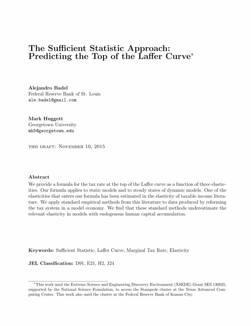
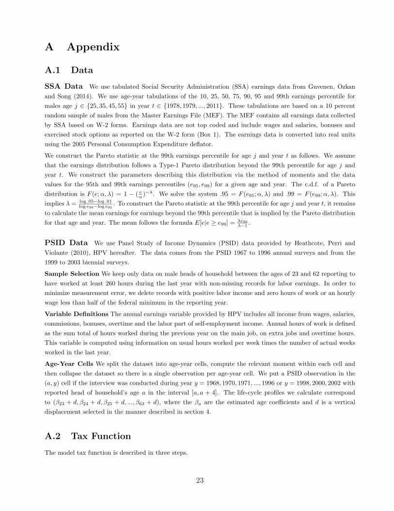
We document properties of the US federal income tax schedule and the US age-earnings dis-
tribution. Figure 1 graphs the US federal marginal income tax rates in 2010. The income
thresholds in Figure 1 for different tax brackets are stated as multiples of average US income
in 2010. The model tax function T is determined by a polynomial.5 Figure 1 shows that
the marginal rates implied by the model tax function closely approximate US federal marginal
rates. We associate the tax function parameter τ with the top tax rate in Figure 1. When the
parameter τ is increased from the benchmark value of τ = 0.35, the tax function T (y; τ) implied
by this new value of τ is unchanged below the top threshold but differs above the threshold.
Thus, the class T of tax functions satisfies assumption A2 from section 2.
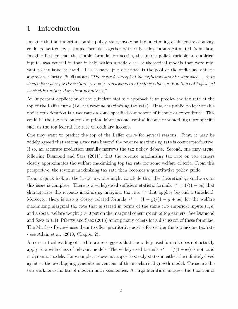
Figure 2 documents earnings and hours facts. The earnings facts are based on the age coef-
ficients from a regression of a third-order polynomial in age and a time dummy variable for
each year run on tabulated US Social Security Administration (SSA) male earnings data from
Guvenen, Ozkan and Song (2014). The earnings facts are (i) median earnings, (ii) the 99-50,
90-50 and 10-50 earnings percentile ratios and (iii) the Pareto statistic. The facts on the average
fraction of time spent working are from Panel Study of Income Dynamics (PSID) male hours
data from Heathcote, Perri and Violante (2010).6 Appendix A.1 describes what is measured in
the SSA and PSID data sets.7
5Appendix A.2 describes data sources and approximation methods.6The average fraction of time spent working is total work hours per year in PSID data divided by discretionary
time (i.e. 14 hours per day times 365 days per year).7The age coefficients from the regression on earnings data are normalized to pass through the data statistics
at age 45 in 2010, with the exception of median earnings which is normalized to 100 at age 55. The agecoefficients from the PSID hours regression are normalized to pass through the average value across years atage 45 as discussed in Appendix A.1.
14

Table 1 - Benchmark Model Parameter Values
Category Functional Forms Parameter Values
Demographics µj+1 = µj/(1 + n) n = 0.01, J = 40j = 1, ..., 40 (ages 23-62)
Tax System T Figure 1 and Appendix
Preferences u(c, n) = log c+ φn1−1/ν
1−1/νβ = 0.952, φ = .231, ν = 0.25
Human Capital H(h, s, a) = h(1− δ) + a(hs)α (α, δ) = (0.833, 0.00001)Initial Conditions (log h1, log a) ∼ N((µh, µa),Σ) (µh, µa) = (5.03,−1.07)
(σh, σa, ρh,a) = (.789, .407, .242)Note: Parameters for Demographics, the Tax System and that utility function parameter ν are preset without
solving for equilibrium. The remaining parameters are set so that the model equilibrium best matches the facts
in Figure 2. Parameters are rounded to 3 significant digits. The parameters (σh, σa, ρh,a) refer to the standard
deviation of log human capital and log learning ability and the correlation between these log variables.
Figure 2 calculates how the Pareto statistic at the 99th percentile for earnings varies with age.
The Pareto statistic is the mean for observations above a threshold divided by the difference
between this mean and the threshold. We set the threshold to be the 99th percentile for each
age and year in the data set. We highlight the Pareto statistic because the cross-sectional value
of the Pareto statistic is the coefficient a1 in the tax rate formula in Theorem 1. We focus on
the Pareto statistic at the 99th percentile because the top federal tax rate iin 2010 begins at
approximately the 99th percentile of income as displayed in Figure 1.
We specify functional forms for the utility function u, human capital H, the tax function T
and for the distribution of initial conditions. Table 1 presents functional forms and parameter
values. We preset some model parameters. Specifically, we set (w, r, n, J) = (1.0, .04, .01, 40) so
that the wage is normalized to 1, the real interest rate is 4 percent, the population growth rate
is 1 percent and the working lifetime is 40 model periods covering a real-life age of 23 to 62.
We preset the tax function T as described above. Finally, we also preset the utility function
parameter to ν = 0.25. This implies that the model has a constant Frisch elasticity of leisure
with respect to human capital equal to −ν and a Frisch elasticity of total labor time (sj + lj)
equal to ν(nj/(lj + sj)).8 Thus, the model has a Frisch elasticity of total labor time equal to
.375 when ν = .25 and nj/(lj + sj) = 1.5
We set all remaining model parameters (governing preferences, human capital and initial con-
ditions) to minimize the weighted squared deviation of the log of equilibrium model moments
from the log of the data moments in Figure 2. Figure 2 plots the corresponding model econ-
8The standard necessary conditions for a solution to Problem P1 with constant marginal tax rates implythat over the life cycle ∆ log nj = ν[log β(1 + r) − ∆ log hj ]. Thus, after correcting for a trend term, leisuredecreases by ν percent after a 1 percent evolutionary increase in human capital across periods.
15

omy moments that result from this minimization problem.9 Table 1 lists the value of model
parameters.
We stress that the goal of the bench test is not to analyze a rich model that accounts for many
aspects of the US tax system and many aspects of the earnings and hours distribution in US
data. Instead, the bench test highlights whether or not the formula is useful in predicting the
top of the Laffer curve in interesting applications for which the answer is not known in advance.
We analyze a dynamic model because our work claims that the formula applies to both static
and dynamic models. We choose to analyze a dynamic human capital model for two reasons.
First, skill accumulation is a natural explanation for why top earners are disproportionately
age 50 and above - see Figure 2. Second, we hypothesize that current methods for estimating
earnings elasticities that are in wide use in the literature will systematically underestimate the
elasticities that are theoretically relevant for determining the top of the Laffer curve. If true,
then bench testing the formula on a human capital model will be especially valuable as it will
highlight a potential weakness in the current status of a large empirical literature.
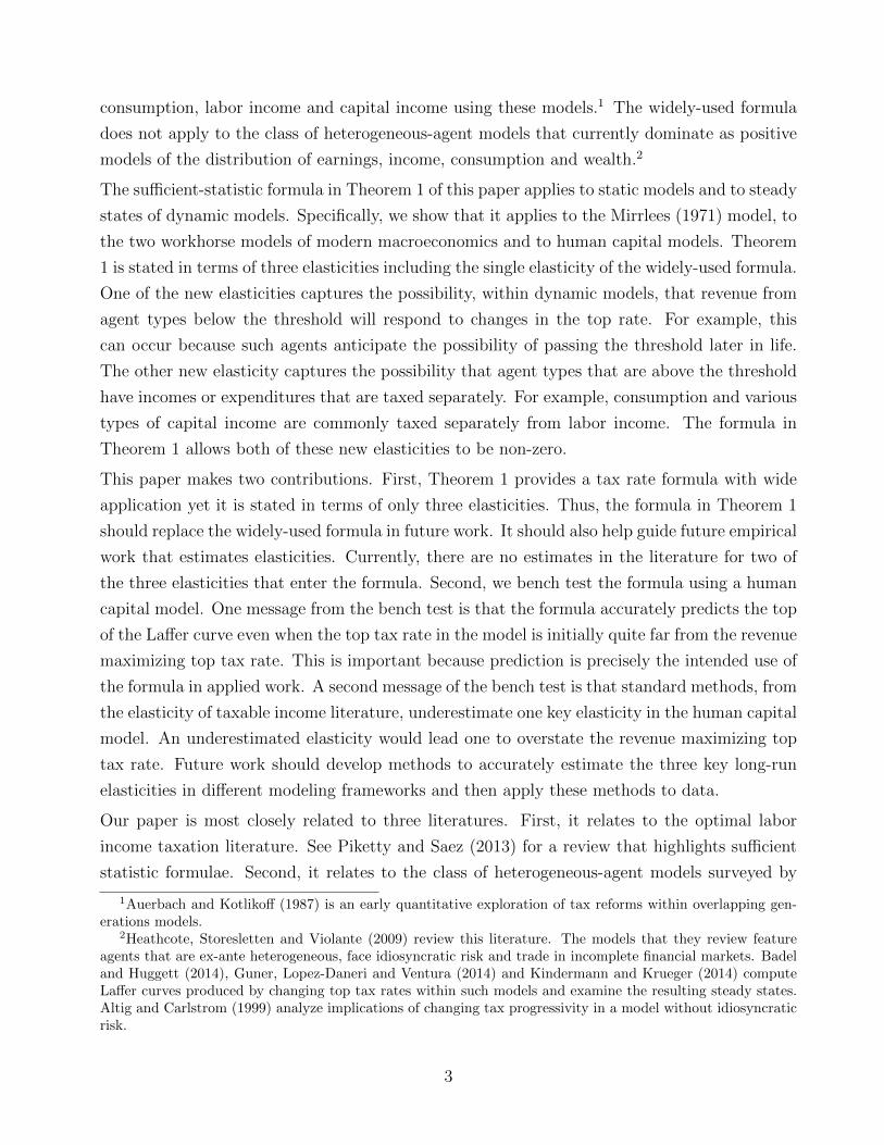
4.3 Theorem 1 and Model Laffer Curves
Figure 3 presents Laffer curves. The Laffer curve for the benchmark model is based on the
parameters in Table 1.10 The Laffer curve for the other model in Figure 3 is based on setting
ν = 0.10 and resetting the remaining model parameters to best match targets following the
procedures for the benchmark model. The goal is to construct model economies where the top
of the Laffer curve occurs at top tax rates that are at varying distances from the initial top
rate in Figure 1. These models are then used to bench test the accuracy of the formula when
the inputs to the formula are calculated away from the maximum.
We now relate the top of the model Laffer curve to the top predicted by the tax rate formula.
To do this, we map equilibrium variables into the language used in Theorem 1. Agent types
have to be defined in terms of exogenous variables to apply Theorem 1. A natural formulation
is that an agent type is x = (h1, a, j) and is determined by the initial condition (h1, a) and age
j.
Step 1: x = (h1, a, j) ∈ X = R+ ×R+ × {1, ..., J}9There is a tension in choosing model parameters governing initial conditions. For example, increasing the
variance of log learning ability σ2a tends to reduce the model Pareto statistic at the 99th percentile but increase
the 99-50 ratio in Figure 2. We conjecture that a more flexible class of distributions over initial conditions iskey to a better fit to the upper tail of the earnings distribution.
10The model Laffer curve is calculated by varying the top tax rate τ , computing the model equilibrium foreach value of τ and plotting the resulting equilibrium total tax revenue. Transfers per agent equal total taxesper agent as implied by the government budget constraint.
16
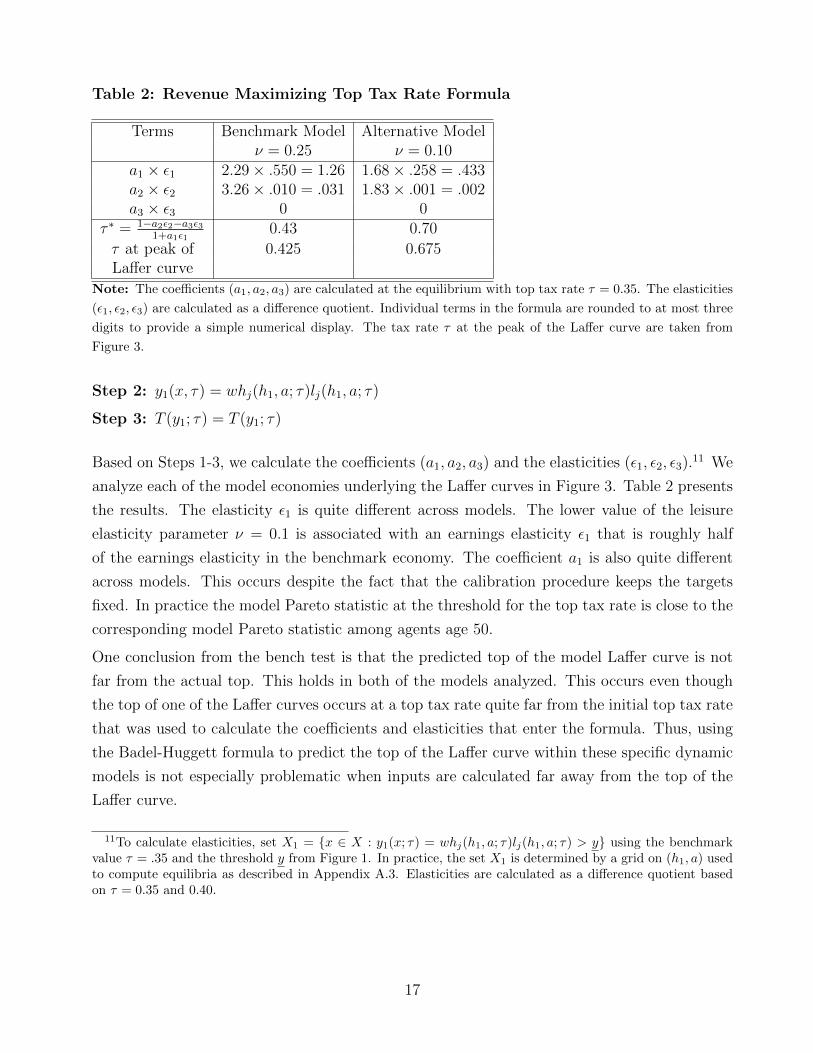
Table 2: Revenue Maximizing Top Tax Rate Formula
Terms Benchmark Model Alternative Modelν = 0.25 ν = 0.10
a1 × ε1 2.29× .550 = 1.26 1.68× .258 = .433a2 × ε2 3.26× .010 = .031 1.83× .001 = .002a3 × ε3 0 0
τ ∗ = 1−a2ε2−a3ε31+a1ε1
0.43 0.70
τ at peak of 0.425 0.675Laffer curve
Note: The coefficients (a1, a2, a3) are calculated at the equilibrium with top tax rate τ = 0.35. The elasticities
(ε1, ε2, ε3) are calculated as a difference quotient. Individual terms in the formula are rounded to at most three
digits to provide a simple numerical display. The tax rate τ at the peak of the Laffer curve are taken from
Figure 3.
Step 2: y1(x, τ) = whj(h1, a; τ)lj(h1, a; τ)
Step 3: T (y1; τ) = T (y1; τ)
Based on Steps 1-3, we calculate the coefficients (a1, a2, a3) and the elasticities (ε1, ε2, ε3).11 We
analyze each of the model economies underlying the Laffer curves in Figure 3. Table 2 presents
the results. The elasticity ε1 is quite different across models. The lower value of the leisure
elasticity parameter ν = 0.1 is associated with an earnings elasticity ε1 that is roughly half
of the earnings elasticity in the benchmark economy. The coefficient a1 is also quite different
across models. This occurs despite the fact that the calibration procedure keeps the targets
fixed. In practice the model Pareto statistic at the threshold for the top tax rate is close to the
corresponding model Pareto statistic among agents age 50.
One conclusion from the bench test is that the predicted top of the model Laffer curve is not
far from the actual top. This holds in both of the models analyzed. This occurs even though
the top of one of the Laffer curves occurs at a top tax rate quite far from the initial top tax rate
that was used to calculate the coefficients and elasticities that enter the formula. Thus, using
the Badel-Huggett formula to predict the top of the Laffer curve within these specific dynamic
models is not especially problematic when inputs are calculated far away from the top of the
Laffer curve.
11To calculate elasticities, set X1 = {x ∈ X : y1(x; τ) = whj(h1, a; τ)lj(h1, a; τ) > y} using the benchmarkvalue τ = .35 and the threshold y from Figure 1. In practice, the set X1 is determined by a grid on (h1, a) usedto compute equilibria as described in Appendix A.3. Elasticities are calculated as a difference quotient basedon τ = 0.35 and 0.40.
17
4.4 Comparing Model Elasticities to Estimated Elasticities
Saez, Slemrod and Giertz (2012) review the literature that estimates earnings or income elastic-
ities with respect to the net-of-tax rate. Much of the literature applies the regression framework
below. The parameter ε is the elasticity with respect to the net-of-tax rate, zit is income or
earnings of individual i at time t, τt(zit) is the marginal tax rate at time t that corresponds to
income zit, f(zit) = log zit is an income control and αt are time dummy variables. The variable
(1− τt(zit)) is refered to as the net-of-tax rate. This regression framework was used by Gruber
and Saez (2002) among many others.
log
(zit+1
zit
)= ε log
(1− τt+1(zit+1)
1− τt(zit)
)+ βf(zit) + αt + νit+1
We follow the literature and apply this regression framework. Unlike the literature, we apply
it to a tax reform within the benchmark human capital model. In model period 1 and 2 agents
live in the economy with top tax rate τ = 0.35 set to the value in the benchmark model. In
model period 3 agents are surprised to discover that the top tax rate is permanently changed
to τ = 0.45. We analyze the tax reform assuming that transfers are constant at the initial
steady-state level. We draw a sample of 30,000 agents between the ages of 23-55 that have
earnings within the top 10 percent of the earnings distribution. We follow these agents for 7
model periods. Model period 3 is the year of the tax reform.
We run the regression above on this sample. We estimate the elasticity using the three different
instrumental variables procedures described and employed in Saez, Slemrod and Giertz (2012,
Table 2). The precise instruments employed are described in Table 3. Table 3 presents the
mean and the standard deviation of the estimated elasticity after applying this framework to
100 different randomly drawn balanced panels of 30,000 agents. The main finding is that the
mean of the estimated elasticities are consistently far below the true long-run model elasticity.
Moreover, standard errors are quite small so that sampling variability is not the explanation
for why estimated elasticities are below long-run elasticities. The reader should keep in mind
that the long-run model elasticity enters the sufficient statistic formula and accurately predicts
the tax rate at the top of the Laffer curve.
5 Discussion
This paper has two main contributions. First, the formula in Theorem 1 applies broadly to
static models and to steady states of dynamic models and yet depends on only three elasticities.
Thus, this sufficient-statistic formula should replace the widely-used formula in future work.
18
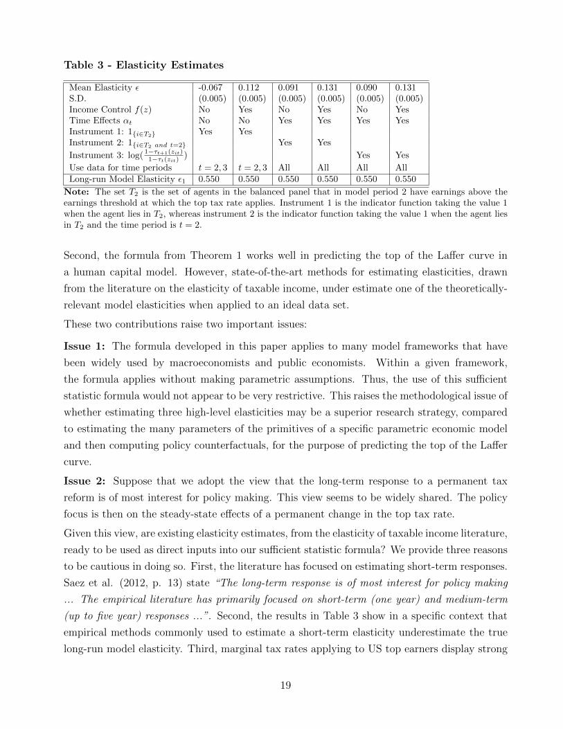
Table 3 - Elasticity Estimates
Mean Elasticity ε -0.067 0.112 0.091 0.131 0.090 0.131S.D. (0.005) (0.005) (0.005) (0.005) (0.005) (0.005)Income Control f(z) No Yes No Yes No YesTime Effects αt No No Yes Yes Yes YesInstrument 1: 1{i∈T2} Yes YesInstrument 2: 1{i∈T2 and t=2} Yes Yes
Instrument 3: log( 1−τt+1(zit)1−τt(zit) ) Yes Yes
Use data for time periods t = 2, 3 t = 2, 3 All All All AllLong-run Model Elasticity ε1 0.550 0.550 0.550 0.550 0.550 0.550
Note: The set T2 is the set of agents in the balanced panel that in model period 2 have earnings above theearnings threshold at which the top tax rate applies. Instrument 1 is the indicator function taking the value 1when the agent lies in T2, whereas instrument 2 is the indicator function taking the value 1 when the agent liesin T2 and the time period is t = 2.
Second, the formula from Theorem 1 works well in predicting the top of the Laffer curve in
a human capital model. However, state-of-the-art methods for estimating elasticities, drawn
from the literature on the elasticity of taxable income, under estimate one of the theoretically-
relevant model elasticities when applied to an ideal data set.
These two contributions raise two important issues:
Issue 1: The formula developed in this paper applies to many model frameworks that have
been widely used by macroeconomists and public economists. Within a given framework,
the formula applies without making parametric assumptions. Thus, the use of this sufficient
statistic formula would not appear to be very restrictive. This raises the methodological issue of
whether estimating three high-level elasticities may be a superior research strategy, compared
to estimating the many parameters of the primitives of a specific parametric economic model
and then computing policy counterfactuals, for the purpose of predicting the top of the Laffer
curve.
Issue 2: Suppose that we adopt the view that the long-term response to a permanent tax
reform is of most interest for policy making. This view seems to be widely shared. The policy
focus is then on the steady-state effects of a permanent change in the top tax rate.
Given this view, are existing elasticity estimates, from the elasticity of taxable income literature,
ready to be used as direct inputs into our sufficient statistic formula? We provide three reasons
to be cautious in doing so. First, the literature has focused on estimating short-term responses.
Saez et al. (2012, p. 13) state “The long-term response is of most interest for policy making
... The empirical literature has primarily focused on short-term (one year) and medium-term
(up to five year) responses ...”. Second, the results in Table 3 show in a specific context that
empirical methods commonly used to estimate a short-term elasticity underestimate the true
long-run model elasticity. Third, marginal tax rates applying to US top earners display strong
19

mean reversion. Mertens (2015) uses proxies for exogenous variation in tax rates to argue that
shocks to US marginal tax rates for the top 1 percent lead to transitory movements in top
tax rates in practice. This raises the important issue of how to estimate long-run elasticities
corresponding to a permanent change in the top tax rate when some of the exogenous variation
in top marginal rates highlighted in the data lead to only transitory movements in these tax
rates.
20
References
1. S. Adam, T. Besley, R. Blundell, S. Bond, R. Chote, M. Grammie, P. Johnson, G. Myles
and J. Poterba (eds.)(2010), Dimensions of Tax Design: The Mirrlees Review, Oxford
University Press, Oxford, UK.
2. Altig, D. and C. Carlstrom (1999), Marginal Tax Rates and Income Inequality in a Life-
Cycle Model, American Economic Review, 89, 1197-1215.
3. Alvaredo, F., Atkinson, A., Piketty, T. and E. Saez, The World Top Incomes Database,
http://topincomes.g-mond.parisschoolofeconomics.eu/ .
4. Auerbach, A. and L. Kotlikoff (1987), Dynamic Fiscal Policy, Cambridge University Press,
Cambridge.
5. Badel, A. and M. Huggett (2014), Taxing Top Earners: A Human Capital Perspective,
manuscript.
6. Ben-Porath, Y. (1967), The Production of Human Capital and the Life Cycle of Earnings,
Journal of Political Economy, 75, 352-65.
7. Chetty, R. (2009), Sufficient Statistics for Welfare Analysis: A Bridge Between Structural
and Reduced-Form Methods, Annual Review of Economics, 1, 451- 88.
8. Diamond, P. (1965), National Debt in a Neoclassical Growth Model, American Economic
Review, 55, 1126- 50.
9. Diamond, P. and E. Saez (2011), The Case for a Progressive Tax: From Basic Research
to Policy Recommendations, Journal of Economic Perspectives, 25, 165-90.
10. Golosov, M., Tsyvinski, A. and N. Werquin (2014), A Variational Approach to the Anal-
ysis of Tax Systems, manuscript.
11. Gruber, J. and E. Saez (2002), The Elasticity of Taxable Income: Evidence and Implica-
tions, Journal of Public Economics, 84, 1-32.
12. Guner, N., Lopez-Daneri, M. and G. Ventura (2014), Heterogeneity and Government
Revenues: Higher Taxes at the Top?, manuscript.
13. Guvenen, F., Ozkan, S. and J. Song (2014), The Nature of Countercyclical Income Risk,
Journal of Political Economy, 122, 621-60.
21
14. Heathcote, J., Storesletten, K. and G. Violante (2009), Quantitative Macroeconomics
with Heterogeneous Households, Annual Review of Economics, 1, 319-54.
15. Heathcote, J, Perri, F. and G. Violante (2110), Unequal We Stand: An Empirical Analysis
of Economic Inequality in the United States: 1967-2006, Review of Economic Dynamics,
13, 15-51.
16. Huggett, M., Ventura, G. and A. Yaron (2006), Human Capital and Earnings Distribution
Dynamics, Journal of Monetary Economics, 53, 265- 90.
17. Kindermann, F. and D. Krueger (2014), High Marginal Tax Rates on the Top 1% ?
Lessons from a Life Cycle Model with Idiosyncratic Income Risk, manuscript.
18. Mertens, K. (2015), Marginal Tax Rates and Income: New Time Series Evidence, manuscript.
19. Mirrlees, J. (1971), An Exploration into the Theory of Optimum Income Taxation, Review
of Economic Studies, 38, 175- 208.
20. Neal, D. and S. Rosen (2000), Theories of the Distribution of Earnings, Handbook of
Income Distribution, (eds) Atkinson and Bourguignon.
21. Piketty, T and E. Saez (2013), Optimal Labor Income Taxation, Handbook of Public
Economics, Volume 5, editors A. Auerbach, R. Chetty, M. Feldstein and E. Saez, Elsevier.
22. Rubinstein, Y. and Y. Weiss (2006), Post Schooling Wage Growth: Investment, Search
and Learning, Handbook of the Economics of Education, (eds) Hanushek and Welch.
23. Saez, E., Slemrod, J. and S. Giertz (2012), The Elasticity of Taxable Income with Respect
to Marginal Tax Rates: A Critical Review, Journal of Economic Literature, 50:1, 3-50.
24. Trabandt, M. and H. Uhlig (2011), The Laffer Curve Revisited, Journal of Monetary
Economics, 58, 305- 27.
25. Weiss, Y. (1986), The Determination of Life Cycle Earnings: A Survey, Handbook of
Labor Economics, (eds) Ashenfelter and Layard, Elsevier.
22
A Appendix
A.1 Data
SSA Data We use tabulated Social Security Administration (SSA) earnings data from Guvenen, Ozkan
and Song (2014). We use age-year tabulations of the 10, 25, 50, 75, 90, 95 and 99th earnings percentile for
males age j ∈ {25, 35, 45, 55} in year t ∈ {1978, 1979, ..., 2011}. These tabulations are based on a 10 percent
random sample of males from the Master Earnings File (MEF). The MEF contains all earnings data collected
by SSA based on W-2 forms. Earnings data are not top coded and include wages and salaries, bonuses and
exercised stock options as reported on the W-2 form (Box 1). The earnings data is converted into real units
using the 2005 Personal Consumption Expenditure deflator.
We construct the Pareto statistic at the 99th earnings percentile for age j and year t as follows. We assume
that the earnings distribution follows a Type-1 Pareto distribution beyond the 99th percentile for age j and
year t. We construct the parameters describing this distribution via the method of moments and the data
values for the 95th and 99th earnings percentiles (e95, e99) for a given age and year. The c.d.f. of a Pareto
distribution is F (e;α, λ) = 1 − ( eα )−λ. We solve the system .95 = F (e95;α, λ) and .99 = F (e99;α, λ). This
implies λ = log .05−log .01log e99−log e95 . To construct the Pareto statistic at the 99th percentile for age j and year t, it remains
to calculate the mean earnings for earnings beyond the 99th percentile that is implied by the Pareto distribution
for that age and year. The mean follows the formula E[e|e ≥ e99] = λe99λ−1 .
PSID Data We use Panel Study of Income Dynamics (PSID) data provided by Heathcote, Perri and
Violante (2010), HPV hereafter. The data comes from the PSID 1967 to 1996 annual surveys and from the
1999 to 2003 biennial surveys.
Sample Selection We keep only data on male heads of household between the ages of 23 and 62 reporting to
have worked at least 260 hours during the last year with non-missing records for labor earnings. In order to
minimize measurement error, we delete records with positive labor income and zero hours of work or an hourly
wage less than half of the federal minimum in the reporting year.
Variable Definitions The annual earnings variable provided by HPV includes all income from wages, salaries,
commissions, bonuses, overtime and the labor part of self-employment income. Annual hours of work is defined
as the sum total of hours worked during the previous year on the main job, on extra jobs and overtime hours.
This variable is computed using information on usual hours worked per week times the number of actual weeks
worked in the last year.
Age-Year Cells We split the dataset into age-year cells, compute the relevant moment within each cell and
then collapse the dataset so there is a single observation per age-year cell. We put a PSID observation in the
(a, y) cell if the interview was conducted during year y = 1968, 1970, 1971, ..., 1996 or y = 1998, 2000, 2002 with
reported head of household’s age a in the interval [a, a + 4]. The life-cycle profiles we calculate correspond
to (β23 + d, β24 + d, β25 + d, ..., β63 + d), where the βa are the estimated age coefficients and d is a vertical
displacement selected in the manner described in section 4.
A.2 Tax Function
The model tax function is described in three steps.
23

Step 1: Specify the empirical tax function T (x):
T (x) =
R1[x− q1] i(x) = 1∑i(x)n=2Rn−1[qn − qn−1] +Ri(x)[x− qi(x)] i(x) > 1
i(x) ≡ maxn s.t. n ∈ {1, 2, ..., N} and qn ≤ x
The values {(q1, R1), ..., (q7, R7)} are set based on the seven tax brackets and tax rates for the 2010 federal
income tax schedule for married couples filing jointly. Brackets and rates come from Schedule Y-1 in the IRS
Form 1040 Instructions. Adding $18, 700 to each of the taxable income brackets from Schedule Y-1 generates
total income cutoffs that produce these taxable income cutoffs in Schedule Y-1 for joint filers without dependents
according to the NBER tax program TAXSIM for the 2010 tax year. Total income brackets qn are stated as
multiples of average income in 2010.12
Step 2: Fit the 5th order polynomial P (x; ζ) to T (x):
ζ ∈ argmin∑
xi∈Xgrid
(T (xi)− P (xi; ζ))2 subject to P (0; ζ) = 0, P ′(q7; ζ) = 0.35
Xgrid contains 51 points uniformly distributed on the interval [0, q7].
Step 3: Set the model tax function(s) T (e; τ):
T (e; τ) =
eP (e/e; ζ) e ≤ q7e
eP (q7; ζ) + τ [e− q7e] e > q7e
The quantity e is average earnings in the model. Note that P (x; ζ) from Step 2 takes input x stated in multiples
of average income and states output in units of average income.
A.3 Computation
The algorithm to compute the model Laffer curve is given below. This computation takes all model parameters
and the structure of the tax system below the threshold as given. The tax system below the threshold is
expressed as a function of e as described in Appendix A.2. Thus, to compute the Laffer curve we fix the value
e at its value in the benchmark model.
Algorithm:
1. Guess transfers Tr(τ) for any top tax rate τ ≥ 0.35.
2. Solve Problem DP-1, given Tr(τ).
12The World Top Incomes Database reports that average income per tax unit in 2010 is 53, 347 stated in 2014dollars. Using the CPI, this is equivalent to 49, 278 dollars in 2010. The US top bracket starts at a ratio oftotal income to average income equal to q7 = (373, 650 + 18, 700)/49, 278 = 7.96, where 373, 650 is the start ofthe top taxable income bracket and 18, 700 is the standard deduction for joint filers without dependents.
24

3. Compute the implied values of Tr(τ) using the optimal decision rules from step 2 and a discretized initial
distribution. If the guessed and implied values are within tolerance, then stop. Otherwise, revise the
guess and repeat steps 2-3.
We solve Problem 1 by solving the dynamic programming problem DP-1 below. For each age and state (h, k, a)
on a grid, we solve an inner and an outer problem. The inner problem takes choices (k′, s) as given and solves for
(c, l). The inner problem is easy to solve by bisection. This is true when T is differentiable almost everywhere
and T ′ is increasing. The class of model tax functions satisfies both properties. The outer problem maximizes
over (k′, s), using solutions to the inner problem. The outer problem is solved by a Nelder-Mead algorithm.
(DP − 1) vj(h, k, a) = max u(c, 1− s− l) + βvj+1(h′, k′, a) subject to
c+ k′ ≤ whl + k(1 + r)− T (whl) , c, s, l, k′ ≥ 0, 0 ≤ s+ l ≤ 1 and h′ = H(h, s, a)
To compute the implied value of Tr(τ), we use a discrete approximation to the bivariate lognormal N(µ,Σ).
We use 16 points for log a and 61 points for log h1. The grid points for log a and log h1 range from 3.99 standard
deviations above and below the mean of the respective marginal distributions. For learning ability, we put 8
points below the 90th percentile and 8 points above the 90th percentile.
25
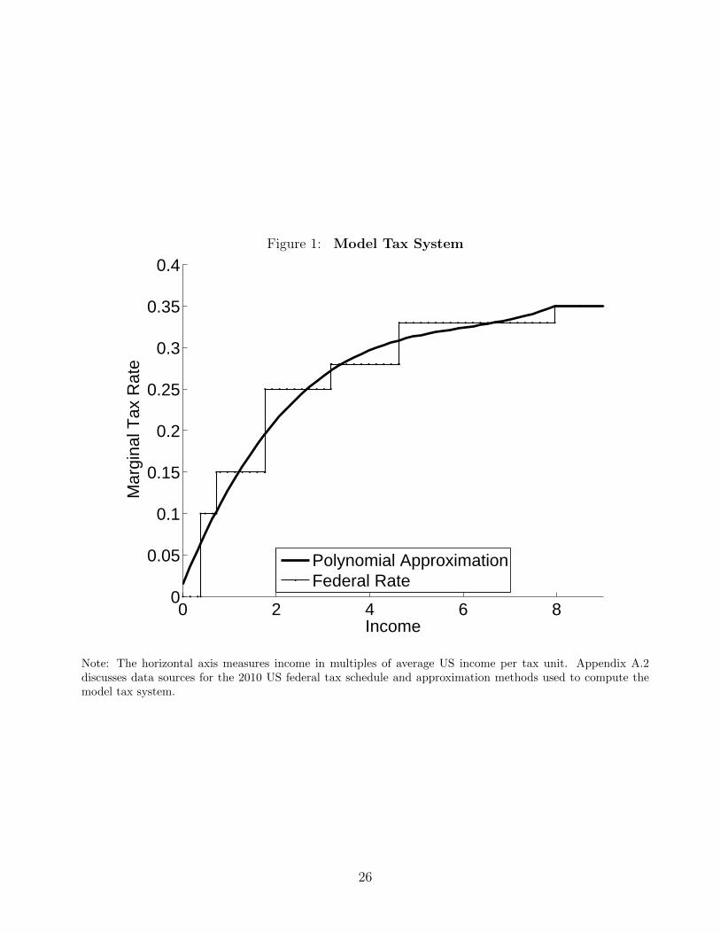
Figure 1: Model Tax System
0 2 4 6 80
0.05
0.1
0.15
0.2
0.25
0.3
0.35
0.4
Income
Mar
gina
l Tax
Rat
e
Polynomial ApproximationFederal Rate
Note: The horizontal axis measures income in multiples of average US income per tax unit. Appendix A.2discusses data sources for the 2010 US federal tax schedule and approximation methods used to compute themodel tax system.
26
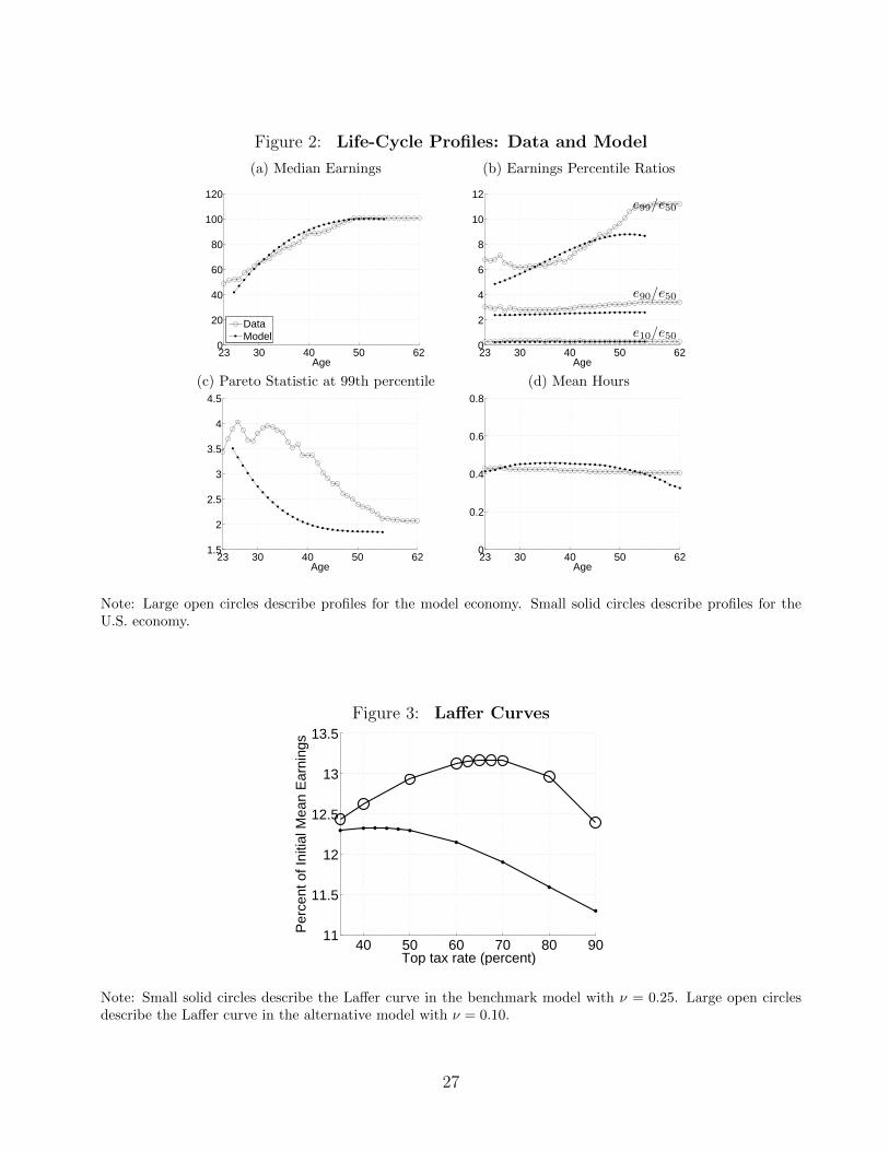
Figure 2: Life-Cycle Profiles: Data and Model
(a) Median Earnings (b) Earnings Percentile Ratios
23 30 40 50 620
20
40
60
80
100
120
Age
DataModel
23 30 40 50 620
2
4
6
8
10
12
Age
e90/e50
e10/e50
e99/e50
(c) Pareto Statistic at 99th percentile (d) Mean Hours
23 30 40 50 621.5
2
2.5
3
3.5
4
4.5
Age23 30 40 50 620
0.2
0.4
0.6
0.8
Age
Note: Large open circles describe profiles for the model economy. Small solid circles describe profiles for theU.S. economy.
Figure 3: Laffer Curves
40 50 60 70 80 9011
11.5
12
12.5
13
13.5
Per
cent
of I
nitia
l Mea
n E
arni
ngs
Top tax rate (percent)
Note: Small solid circles describe the Laffer curve in the benchmark model with ν = 0.25. Large open circlesdescribe the Laffer curve in the alternative model with ν = 0.10.
27