Some illustrative examples on the

analysis of the SW-CRT

30/08/2016

Karla Hemming

Calendar time is a confounder

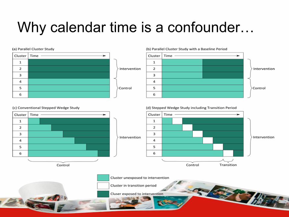
Why calendar time is a confounder…

Time effects

• When designing a SW-CRT time needs to

be allowed for in the sample size

calculation.

• Time also needs to be allowed for in the

analysis

Analysis

Analysis • Summarise key characteristics by exposure / unexposed status

– Identify selection biases

• Analysis either GEE or mixed models

– Clustering

– Time effects

• Imbalance of calendar time between exposed / unexposed:

– The majority of the control observations will be before the

majority of the intervention observations

– Time is a confounder!

• Unadjusted effect meaningless

Treatment effect

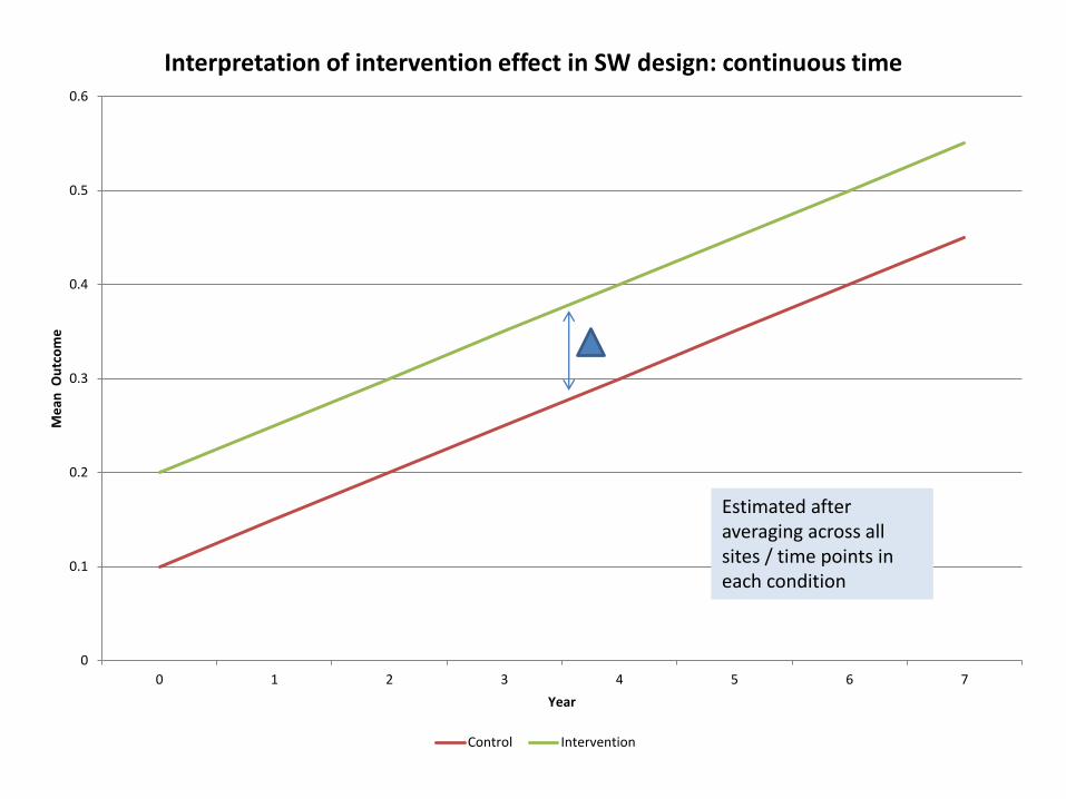
• After accounting for any secular changes, what is the effect of the intervention, averaged across steps?

• The intervention effect is modelled as a change in level, constant across steps (or time)

0

0.1

0.2

0.3

0.4

0.5

0.6

0 1 2 3 4 5 6 7

Me

an O

utc

om

e

Year

Interpretation of intervention effect in SW design: continuous time

Control Intervention

Estimated after averaging across all sites / time points in each condition

0

0.05

0.1

0.15

0.2

0.25

0.3

0.35

0.4

1 2 3 4 5 6 7 8

Me

an o

utc

om

e

Year

Interpretation of intervention effect in SW: categorical time

Control

Intervention

Example one

11

Example 1: Maternity sweeping

• Objective: evaluate a training scheme to improve the rate of membrane sweeping in post term pregnancies

– Primary outcome:• Proportion of women having a membrane sweep

• Baseline rate 40%

• Hope to increase to 50% during 12 weeks post intervention

– Cluster design:• 10 teams (clusters); 12 births per cluster per week

• Pragmatic design – rolled out when possible

• Transition period to allow training

12

Example 1: Maternity sweeping

(transition period)

Example 1: Underlying trend 0

.2.4

.6.8

Prop

. wom

en sw

ept (

95%

CI)

20005/03/12 23/04/12 18/06/12 13/08/12week commencing

Example 1: results

Unexposed

to

intervention

n=1417

Exposed to

intervention

n=1356

Relative Risk P-

value

Number of women offered and accepting membrane sweeping

Number (%) 629 (44.4%) 634 (46.8%)

Cluster adjusted 1.06 (0.97, 1.16) 0.21

Time and cluster adjusted

Fixed effects time 0.88 (0.69, 1.05) 0.11

Linear time effect 0.90 (0.73, 1.11) 0.34

Example 1: Impact of secular trend0

.2.4

.6.8

Prop

. wom

en sw

ept (

95%

CI)

20005/03/12 23/04/12 18/06/12 13/08/12week commencing

Unadjusted RR = 1.06 95% CI (0.97, 1.16)

Adjusted (for time) RR = 0.88 95% CI (0.69, 1.05)

Rising Tide?

Contamination?

Explanations

• Rising tide

– General move towards improving care – perhaps due

to very initiative that prompted study investigators to

do this study

• Contamination

– Unexposed clusters became exposed before their

randomisation date

• Lack of precision

– Intervention wasn’t ruled out as being effective

Example 2

Example 2: Critical care outreach

• Intervention: Critical care outreach

• Setting: Hospital in Iran

• Clusters: Wards

• Outcome: Mortality

Example 2: Design

Example 2: Underlying trend0

.05

.1.1

5

Prop

. of d

eath

s (9

5% C

I)

07/10 04/1111/10 09/11Study epoch (each epoch represents a four week period)

Example 2: results

Unexposed to

intervention

Exposed to

interventionTreatment effect P-value

Number of Patients 7,802 10,880

Mortality

Number (%) 370 (4.74) 384 (3.53) OR (95% CI)

Unadjusted 0.73 (0.64, 0.85) 0.000

Cluster adjusted 1.02 (0.83, 1.26) 0.817

Fixed effects for time 0.82 (0.56, 1.19) 0.297

Linear effect for time 0.96 (0.76, 1.22) 0.750

Covariate adjusted 0.97 (0.64, 1.47) 0.489

Example 2: Underlying trend0

.05

.1.1

5

Prop

. of d

eath

s (9

5% C

I)

07/10 04/1111/10 09/11Study epoch (each epoch represents a four week period)

Unadjusted OR = 1.02 95% CI (0.83, 1.26)

Adjusted OR = 0.82 95% CI (0.56,1.19)

Lack of power?

Explanations

• Rising tide

– General move towards improving care – perhaps due

to very initiative that prompted study investigators to

do this study

• Contamination

– Unexposed clusters became exposed before their

randomisation date

• Lack of precision

– Intervention wasn’t ruled out as being effective

Models fitted

• Mixed effects model

• Random effect for cluster

• Fixed effect for time and intervention

𝑌𝑖𝑗𝑙 = 𝜇 + 𝛽𝑗 + θ𝑋𝑖𝑗 + 𝑢𝑖 + 𝑒𝑖𝑗𝑙

𝑢𝑖~𝑁 0, 𝜎𝑏 ; 𝑒𝑖𝑗𝑙 ~𝑁(0, 𝜎𝑤)

(time j, cluster i, individual l )

Parameter estimation

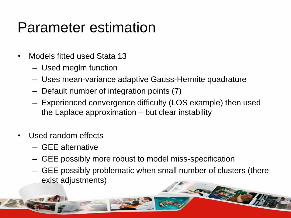
• Models fitted used Stata 13

– Used meglm function

– Uses mean-variance adaptive Gauss-Hermite quadrature

– Default number of integration points (7)

– Experienced convergence difficulty (LOS example) then used

the Laplace approximation – but clear instability

• Used random effects

– GEE alternative

– GEE possibly more robust to model miss-specification

– GEE possibly problematic when small number of clusters (there

exist adjustments)

Model assumptions and extensions

Model assumptions 1

• Underlying secular trend

– The underlying secular trend is same across all clusters

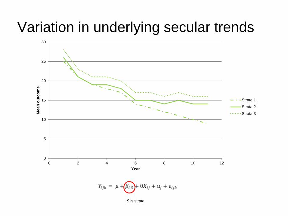
Variation in underlying secular trends

S is strata

0

5

10

15

20

25

30

0 2 4 6 8 10 12

Mean

ou

tco

me

Year

Strata 1

Strata 2

Strata 3

Model assumptions 2

• Time invariant treatment effect

– There is no delayed intervention effect

– No change in intensity of the effect over the course of time

– No time by treatment interaction

– Time (since introduction) isn't an effect modifier

Time variant treatment effect

𝑌𝑖𝑗𝑙 = 𝜇 + 𝛽𝑗 + 𝜃𝑗𝑋𝑖𝑗 + 𝑢𝑖 + 𝑒𝑖𝑗𝑙

0

5

10

15

20

25

30

1 2 3 4 5 6 7 8

Me

an o

utc

om

e

Year

Control

Intervention

Model assumptions 3

• Intra cluster correlation

– The correlation between two individuals is independent of time

– Two observations in the same cluster / time period have the

same degree of correlation as two observations in the same

cluster but different time periods

Time𝑌𝑖𝑗𝑙 = 𝜇 + 𝛽𝑗 + θ𝑋𝑖𝑗 + 𝑢𝑖 + 𝑣𝑖𝑗 + 𝑒𝑖𝑗𝑙

𝑢𝑖~𝑁 0, 𝜎𝑏 ; 𝑣𝑖𝑗~𝑁 0, 𝜎𝑣 ; 𝑒𝑖𝑗𝑙 ~𝑁(0, 𝜎𝑤)

Model assumptions 4

• Treatment effect heterogeneity

– The effect of the intervention is the same across all clusters

– Typical assumption in CRTs

– In a meta-analysis common to assume between cluster

heterogeneity in treatment effect

𝑌𝑖𝑗𝑙 = 𝜇 + 𝛽𝑗 + 𝜃𝑖𝑋𝑖𝑗 + 𝑢𝑖 + 𝑒𝑖𝑗𝑙

𝜃𝑖 ~𝑁(𝜃, 𝜎𝜃)

Summary

• Time is a potential partial confounder

• Designs which are completely confounded with time shouldn’t be

used

• Time must be allowed for as a covariate in primary analysis

• Model extensions require sufficient power and pre-specification

References

• Scott JM, deCamp A, Juraska M, Fay MP, Gilbert PB. Finite-sample

corrected generalized estimating equation of population average treatment

effects in stepped wedge cluster randomized trials. Stat Methods Med Res.

2014 Sep 29. pii: 0962280214552092. [Epub ahead of print] PubMed PMID:

25267551.

• Ukoumunne OC, Carlin JB, Gulliford MC. A simulation study of odds ratio

estimation for binary outcomes from cluster randomized trials. Stat Med.

2007 Aug 15;26(18):3415-28. PubMed PMID: 17154246.

• Heo M, Leon AC. Comparison of statistical methods for analysis of

clustered binary observations. Stat Med. 2005 Mar 30;24(6):911-23.

PubMed PMID: 15558576