the social costs of an mtbe ban in california · the social costs of an mtbe ban in california ......
TRANSCRIPT
THE SOCIAL COSTS OF AN MTBE BAN IN CALIFORNIA
THE AUTHORS WISH TO THANK LYONDELL CHEMICAL COMPANY FOR FINANCIAL SUPPORT OF THEIR RESEARCH. THE VIEWS AND OPINIONS EXPRESSED HEREIN ARE THOSE OF THE AUTHORS AND MAY NOT REPRESENT THE VIEWS AND OPINIONS OF LYONDELL CHEMICAL COMPANY.

The Social Costs of an MTBE Ban in California
i CHARLES RIVER ASSOCIATES
TABLE OF CONTENTS
Executive Summary .................................................................................................................. 1
The Social Costs of an MTBE Ban in California............................................................................ 3 1. Introduction............................................................................................................. 3 2. Federal and California Regulations Affecting Gasoline ......................................... 6
2.1 Federal Reformulated Gasoline .............................................................................. 6 2.2 California Cleaner Burning Gasoline...................................................................... 7 2.3 California’s Waiver Request ................................................................................. 10 2.4 EPA Rulemaking on MTBE ................................................................................. 12 2.5 NAFTA Arbitration............................................................................................... 12 2.6 Pending Legislation............................................................................................... 13
3. RFG Gasoline Formulation Alternatives .............................................................. 14 3.1 Properties of RFG with MTBE ............................................................................. 14 3.2 Properties of RFG with Ethanol............................................................................ 15 3.3 Properties of Non-Oxygenated RFG..................................................................... 17
4. Cost/Benefit Analysis ........................................................................................... 17 4.1 Summary of Cost-Benefit Analysis ...................................................................... 18 4.2 Fuel Alternatives Considered in the Cost-Benefit Model ..................................... 19 4.3 Treatment of Uncertainty in Cost-Benefit Model ................................................. 22 4.4 Changes in Gasoline Production Costs ................................................................. 23
4.4.1 Refinery Costs.............................................................................................. 24 4.4.2 Fuel Economy .............................................................................................. 25 4.4.3 Gasoline Demand......................................................................................... 25 4.4.4 Ethanol Tax Subsidies.................................................................................. 26 4.4.5 Oil Imports ................................................................................................... 27 4.4.6 Natural Gas Markets .................................................................................... 30 4.4.7 Other Fuel Cost Issues ................................................................................. 31
4.5 Impacts on Air Quality.......................................................................................... 34 4.5.1 Effect of Higher Gasoline Costs .................................................................. 34 4.5.2 Effect of Changes in Air Toxics .................................................................. 37
4.6 Water Quality Impacts .......................................................................................... 38 4.6.1 Background on MTBE Impacts on Water Quality....................................... 39 4.6.1.1 Mobility and Biodegradability of MTBE.................................................. 41 4.6.2 Background on Ethanol Impacts on Water Quality ..................................... 42 4.6.3The Impact of MTBE and Ethanol on Water Quality................................... 44
4.7 LUST Sites ............................................................................................................ 44
The Social Costs of an MTBE Ban in California
ii CHARLES RIVER ASSOCIATES
4.8 Wells ......................................................................................................................48 4.9 Pipelines.................................................................................................................49 4.10 Surface Water ......................................................................................................50
5. Conclusion .............................................................................................................51
Appendix A: Quantification of Costs and Benefits .................................................................53
Appendix B: Comparison of CARB Phase 2 And Phase 3 Regulations .................................60
Appendix C: Development of CARB and Federal Reformulated Gasoline Regulations ........61
TABLE OF FIGURES AND TABLES
Table 1: Federally Reformulated Gasoline Areas in California ....................................................63 Table 2: Properties and Specifications for Phase 3 Reformulated Gasoline .................................64
Table 3: Gasoline Composition and Energy Content ....................................................................65 Table 4: Fuel Properties used to Determine Emissions in predictive model .................................66
Table 5: Emission Reductions Relative to Reference Gasoline (%)..............................................67 Table 6: Reductions in Air Toxics (% Change Relative to Reference Fuel) .................................68
Table 7: Health Benefits of Air Toxic Reductions ........................................................................69 Table 8: Benefits of Reduced Driving ...........................................................................................70
Table 9: Monte Carlo (50,000 repetitions) Results for Cost of Ethanol Scenario Relative to Cost of MTBE Scenario.................................................................................................................71
Table 10: Monte Carlo (50,000 repetitions) Results for Cost of Alkylate Scenario Relative to Cost of MTBE Scenario.................................................................................................................72
Table 11: Monte Carlo (50,000 repetitions) Results for Cost of Blended (70%/30%) Ethanol/Alkylate Scenario Relative to Cost of MTBE Scenario ...................................................73
Figure 1: Overview of Fuel Cost Impact of Switching from MTBE.............................................74 Figure 2: Consumer Surplus Loss Due to Higher Gasoline Price .................................................75
Figure 3: Social Cost of Higher Oil Imports..................................................................................76 Figure 4: Social Costs of an Increase in the World Oil Price ........................................................77
Figure 5: Spillover Effects on Natural Gas Markets......................................................................78 Figure 6: Overview of Air Quality Impact of Switching from MTBE..........................................79
Figure 7: Change in Leaking Underground Storage Tank Remediation Costs d Switching from MTBE ..................................................................................................................80
Figure 8: Incremental Change in Well Remediation Costs due to Switching from MTBE ..........81
The Social Costs of an MTBE Ban in California
iii CHARLES RIVER ASSOCIATES
Figure 9: Incremental Change in Pipeline Spill Costs due to Switching from MTBE ................. 82 Figure 10: Incremental Change in Surface Water Costs due to Switching from MTBE.............. 83

The Social Costs of an MTBE Ban in California
1 CHARLES RIVER ASSOCIATES
EXECUTIVE SUMMARY
In the early 1990s, oxygenated gasoline was widely hailed as a solution to many of the nation’s air quality problems. Even though the anticipated air quality benefits of oxygenated gasoline were in fact realized, the large-scale use of MTBE (methyl tertiary butyl ether) as a gasoline oxygenate resulted in adverse impacts to water quality. The use of MTBE exposed in dramatic fashion the fundamental problem of leaking underground storage tanks. As MTBE was detected in water supplies in the late 1990s, public concern intensified and proposals to ban the use of MTBE in gasoline surfaced in several states, most notably in California, which has moved to ban the use of MTBE in gasoline by 2003.
While the widespread use of MTBE has had adverse impacts on water quality, removal of MTBE from gasoline will impose significant costs on society — both in terms of gasoline production costs and prices, as well as possible impacts on air and water quality by fuel blending components that replace MTBE in gasoline. In moving to protect groundwater resources from MTBE, California may force the adoption of gasoline formulations that are, in fact, less beneficial to society. The total social cost of banning MTBE has not been properly evaluated by the studies that have been conducted to date. Many of these studies evaluate only separable components, and those that propose to perform a comprehensive assessment of the costs and benefits are incomplete and internally inconsistent.
In this paper we provide a comprehensive and internally consistent cost-benefit analysis of the gasoline formulation alternatives for California. Our analysis includes several categories of cost that have largely been neglected in the past analyses of MTBE use. These include: (i) the cost to taxpayers of increased ethanol consumption, due to the ethanol tax subsidy; (ii) the increases in the cost of oil imports caused by replacing MTBE volumes with blending components made from other substitutes; (iii) the effects of changes in gasoline prices on gasoline consumption and thus on automobile emissions; and (iv) the potential effect of MTBE substitutes, such as ethanol, on water quality.
Overall, our analysis indicates that the continued use of MTBE in California gasoline has clear and significant benefits relative to either the use of ethanol or the use of non-oxygenated reformulated gasoline (RFG). The increased annual cost resulting from a ban of MTBE in California when ethanol replaces MTBE ranges from $0.92 billion to $1.32 billion, with an expected value of $1.24 billion. When non-oxygenated RFG replaces MTBE, the annual increased costs range from $0.59 billion to $1.02 billion, with an expected value of $0.92 billion. The model results are robust to reasonable ranges of uncertainty; even under the worst case for MTBE and the best case for the other substitutes, it still follows that banning MTBE will lead to an increase in the total cost associated with gasoline use in the state of California.

3 CHARLES RIVER ASSOCIATES
THE SOCIAL COSTS OF AN MTBE BAN IN CALIFORNIA
GORDON C. RAUSSER
UNIVERSITY OF CALIFORNIA, BERKELEY
GREGORY D. ADAMS W. DAVID MONTGOMERY
ANNE E. SMITH
CHARLES RIVER ASSOCIATES
1. INTRODUCTION
In the early 1990s, oxygenated gasoline was widely hailed as a solution to many of the nation’s air quality problems, especially in the so-called federal nonattainment geographic regions. At that time, it was expected that MTBE (methyl tertiary butyl ether), would be widely used as a gasoline oxygenate. Even though the anticipated air quality benefits of oxygenated gasoline were, in fact, realized, the large-scale use of MTBE as a gasoline oxygenate resulted in adverse impacts to water quality. As MTBE was detected in water supplies in the late 1990s, public concern intensified and proposals to ban the use of MTBE in gasoline surfaced in several states.
In 1999, the State of California passed the first legislation in the United States that was motivated by the water quality impacts of MTBE. Under the authority granted by this legislation, the governor of the State of California announced in March 1999 that MTBE would be banned in gasoline in California beginning in 2003.1 Several other states have moved to reduce or eliminate the use of MTBE as well, and the U.S. Environmental Protection Agency (EPA) is evaluating a federal ban on MTBE. At the same time that the State of California moved to ban MTBE, California also requested that the EPA waive the federal minimum oxygenate requirement for reformulated gasoline sold in California. 2 While this request has been denied, 3 California congressional representatives have introduced legislation that would waive the federal oxygenate requirement, with the result that the production and sale of non-oxygenated gasoline would be possible throughout California, as well as the rest of the United States.
1 Governor Gray Davis, Executive Order D-5-99, 25 March 1999. 2 Governor Gray Davis, letter to Carol Browner, 12 April 1999. 3 United States Environmental Protection Agency, “EPA issues decision on California waiver request,” press
release, 12 June 2001; United States Environmental Protection Agency, “Analysis of and Action on California’s Request for a Waiver of the Oxygen Content in Gasoline,” EPA 420-S-01-008, June 2001.
The Social Costs of an MTBE Ban in California
4 CHARLES RIVER ASSOCIATES
As the pendulum has swung from public concern about air quality to public concern about water quality, the risk has increased that special interests will dominate implementation of policy reforms that ill-serve society. Unfortunately, this risk has not been mitigated by the studies that have been conducted to date. Many of these studies evaluate only separable components,4 and those that propose to perform a comprehensive evaluation of the cost and benefits are incomplete and internally inconsistent.5 Given the billions of dollars of potential consequences that can be quantified, it is surprising that the proposed banning of MTBE has not been subjected to a serious and internally consistent analysis.
The purpose of this paper is to better inform those involved in the policy debate by providing a comprehensive and internally consistent cost-benefit analysis of the gasoline formulation alternatives for California, based on the best information that is currently available. Such an analysis must distinguish between sunk and incremental costs,6 and must consider both private and social costs.7 The analysis must also recognize the economic responses of consumers and firms to changes in prices and costs, and must consider not only costs in the immediate market in question, but also costs from spillovers to other markets.
Several categories of cost that are important to any comprehensive cost-benefit analysis have been neglected in the existing literature. These costs include: (i) the cost to taxpayers of increased ethanol consumption, due to the ethanol tax subsidy; (ii) the increases in the cost of
4 See, for instance, California Energy Commission, “Analysis of the Refining Economics of California Phase 3
RFG”; and “An Evaluation of MTBE Impacts to California Groundwater Resources,” Lawrence Livermore National Laboratory.
5 See, for instance, Arturo A. Keller, Linda Fernandez, Samuel Hitz, Heather Kun, Alan Peterson, Britton Smith and Masaru Yoshioka, “An integral cost-benefit analysis of gasoline formulations meeting California Phase 2 Reformulated Gasoline requirements,” Bren School of Environmental Science and Management, UCSB, Santa Barbara, CA, 1998.
6 Sunk costs are those costs that cannot be averted by future action. For instance, the past use of MTBE may result in current sites of groundwater contamination that will result in future remediation costs. However, even if MTBE is removed from gasoline now, this will not affect the (past, current and future) costs from existing contamination sites. Therefore, these remediation costs are not a cost of continuing to use MTBE in gasoline. Only those remediation costs from future releases of gasoline containing MTBE are a cost of the continued use of MTBE.
7 Private costs are costs reflected in the market prices of products. The most obvious example is the change in the price of gasoline faced by consumers. Private costs should also take into account effects in related markets such as natural gas. Other private costs are the less obvious impacts on the effective price of gasoline to consumers, such as changes in the amount of gasoline required to drive a mile attributable to replacement of MTBE with other blending components. Social costs are costs not necessarily included in market prices, or considered by consumers and producers in their decisions on how much to buy and sell. The impact of MTBE on water resources is a social cost. The impact of changes in air quality (and thus on human health) is another example of a social cost. Prior studies have assumed, correctly, that the performance requirements for reformulated gasoline, stated in terms of required reductions in emissions in ozone precursors — nitrogen oxides and reactive hydrocarbons — and carbon monoxide, would not be compromised if there were a ban on MTBE. However, there are differences in the emissions of some air toxics and potential carcinogens among gasoline alternatives, and these differences need to be carefully considered.
The Social Costs of an MTBE Ban in California
5 CHARLES RIVER ASSOCIATES
oil imports caused by replacing MTBE volumes with blending components made from other substitutes; (iii) the effects of changes in gasoline prices on gasoline consumption and thus on automobile emissions; and (iv) the potential effect of MTBE substitutes, such as ethanol, on water quality.
It is also critical to recognize that the incremental costs and benefits of removing MTBE from gasoline change with the passage of time. The use of oxygenated gasoline in the early 1990s was intended to provide rapid reductions in emissions from the existing fleet of vehicles — reductions that could not be achieved through new car emission standards alone. But as vehicles subject to much more stringent new car emission standards have become a larger share of the fleet, the air quality benefits attributable to the use of oxygenated gasoline have fallen. Moreover, new air quality models adopted by the California Air Resources Board (CARB) for evaluating emissions reductions from reformulated gasoline may also significantly change the estimated air quality impacts of various fuel formulations. The costs of replacing MTBE are also different today than they were a decade ago. The U.S. Supreme Court recently upheld a Unocal patent that covers many of the most cost-effective formulas for producing reformulated gasoline, and this patent will raise costs for other refiners and consumers. Effects on water supply and cleanup costs attributable to future MTBE use are also certainly different today than ten years ago. For instance, older underground gasoline storage tanks that were prone to leaks have almost entirely been replaced by new tanks that are much less likely to leak.
Before turning to the cost-benefit framework presented in Section 4, it is useful to review the regulatory history and current environment pertaining to MTBE, and the current feasible alternatives to MTBE. In Section 2, we discuss the regulatory environment affecting gasoline formulation in California. This environment includes federal regulations, State of California regulations, a California request for a waiver of the gasoline-oxygenate requirement of the Clean Air Act Amendments (CAAA), recent U.S. Environmental Protection Agency rule-making regarding MTBE, a pending North American Free Trade Agreement (NAFTA) arbitration and pending legislation that has been introduced in the U.S. Congress. Section 3 then discusses alternative gasoline formulations and the relevant options that are available if an MTBE ban is implemented. The cost benefit analysis is presented in Section 4. Section 5 presents our concluding remarks.
The Social Costs of an MTBE Ban in California
6 CHARLES RIVER ASSOCIATES
2. FEDERAL AND CALIFORNIA REGULATIONS AFFECTING GASOLINE
Under current law, all gasoline sold in the “ozone nonattainment areas” of California is subject to the federal reformulated gasoline program, and must contain a minimum of 2% oxygen by weight. This requirement can be satisfied by a blend that contains either 5.7% ethanol or 11.5% MTBE (by volume). In addition, gasoline sold during winter months in “carbon monoxide nonattainment areas” of California is subject to the federal oxygenated fuel requirement, and must contain at least 1.8% oxygen.
California is authorized under 42 USC Section 7545(c)(4)(B) to craft its own controls on motor vehicle emission and fuels, as long as they are at least as stringent as the national standards. Under this authority, the Air Resources Board has established rules for California cleaner burning gasoline which are more stringent than the federal standards except in the area of oxygenates. The federal reformulated gasoline (RFG) requirements pre-empt California RFG requirements because they set a more stringent standard for oxygenates than do the California regulations.
The original version of the California RFG rule required a minimum of 1.8% oxygen in winter throughout the state, but that rule was revised in 1998 to apply only to areas subject to the federal winter oxygen requirements. The California Air Resources Board recently issued Phase 3 RFG regulations that would allow refiners throughout the state to sell non-oxygenated gasoline even in federal RFG areas should a waiver of the federal requirement be granted. That waiver request was denied in June 2001.
2.1 Federal Reformulated Gasoline
The federal reformulated gasoline program was created by the Clean Air Act Amendments of 1990 (CAAA). Its purpose was in large part to reduce emissions of so-called ozone precursors, particularly hydrocarbons (referred to in the act as volatile organic compounds or VOCs), from the existing fleet of vehicles. In addition, the CAAA set limits on benzene and heavy metals, and required EPA to ensure that nitrogen oxide (NOx) emissions not be allowed to increase. The requirement for use of RFG applies in areas of the country that are not in attainment with the Ozone National Ambient Air Quality Standard. Initially, the nine worst ozone nonattainment areas, including Los Angeles, were subject to the requirement. The requirement also applies to an area one year after it has been reclassified as a “severe ozone nonattainment area,” which led to Sacramento being included in 1998.
The CAAA set up a performance requirement for federal RFG. This regulation required the EPA’s rules to achieve a specified reduction in emissions relative to a baseline gasoline defined by the Act. The performance standards include two “phases.” The initial Phase 1 standard was a 15% reduction in hydrocarbon emissions, on a mass basis. Beginning in 2000,
The Social Costs of an MTBE Ban in California
7 CHARLES RIVER ASSOCIATES
the Phase 2 standards required a 25.9% reduction in hydrocarbons in northern areas and a 27.5% reduction in southern areas, as measured against the baseline gasoline.
In addition to the performance standard, the CAAA stated that reformulated gasoline must contain oxygenates to provide at least 2.0 weight percent oxygen in the fuel. To meet the oxygenate requirements, refiners are permitted to blend into gasoline any of a number of oxygenates, including MTBE, ethanol, ethyl tertiary-butyl ether (ETBE) or tertiary amyl methyl ether (TAME).8 Except for ethanol, all of these oxygenates are ethers. MTBE had already been used in small quantities for a number of years to boost the octane in gasoline, and served primarily as a replacement for lead. Following passage of the CAAA, MTBE became the preferred blending component in California (and other non-Midwest states) for meeting the minimum oxygen requirement in RFG.
Carbon monoxide (CO) nonattainment areas are required under separate provisions of the federal CAAA of 1990 to have oxygenated gasoline during certain winter months. Only the South Coast Air Basin and part of Imperial County are now subject to federal winter oxygenate requirements.
Table 1 lists the counties in California where federal RFG rules currently apply. Since these counties contain a large share of the state’s population, the Air Resources Board estimates that 70% of the gasoline currently sold in California is subject to the federal RFG regulations, including the minimum 2% oxygen requirement.9 Without a change in the CAAA or a waiver of the application of the current federal rules to California, it would be illegal to sell a “non-oxygenated CARB gasoline” within these designated ozone nonattainment areas.
2.2 California Cleaner Burning Gasoline
California is authorized under 42 USC Section 7545(c)(4)(B) to craft its own controls on motor vehicle emission and fuels, as long as they are at least as stringent as the national
8 Since ethanol contains approximately 35% oxygen by weight, a blend that contains 5.7% ethanol meets the
federal requirement. MTBE contains approximately half the amount of oxygen as ethanol, 17% by weight, so that the blend must contain approximately 11% MTBE to meet the federal standard.
9 Jose Gomez, Bill Riddell, Richard Vincent and Tom Jennings, “Staff Report: Initial Statement of Reasons for Proposed Rulemaking,” July 1998.
The Social Costs of an MTBE Ban in California
8 CHARLES RIVER ASSOCIATES
standards. CARB is authorized under state law to establish motor vehicle fuel specifications.10 Under this authority, California has its own reformulated gasoline regulations.11
CARB adopted its Phase 2 RFG regulations in November 1991, and set March 1, 1996 as the date when these regulations would take affect.12 The Phase 2 regulations defined a reference fuel and required that any gasoline sold in California have emissions levels of three specified pollutants that are at least as low as those of the reference fuel. The three specified pollutants are hydrocarbons (HC), nitrogen oxides (NOx), and potency-weighted toxics (PWT). The specifications of the reference fuel include regulations for eight properties, but do not explicitly require that an oxygenate be used in order to meet these standards.13 However, until 1998, CARB regulations did require a statewide 1.8% minimum oxygenate content in winter as part of the California State Implementation Plan (SIP).14 In 1998 CARB replaced the statewide minimum winter oxygenate requirement with a winter oxygenate requirement applicable just to the CO nonattainment areas. Thus, outside these areas, the CARB regulations do not require any minimum oxygen content (although the federal RFG regulations — and the attendant oxygenate requirement — still applied in ozone nonattainment areas).
CARB also developed a predictive model to be used by refiners to determine if a particular gasoline blend would produce emissions levels of the three regulated pollutants that were at least as low as those for the reference fuel. Development of the predictive model began in 1991, and it was adopted by regulation at a hearing in June 1994. California Phase 2 RFG production began on March 1, 1996. Seven of the eight Phase 2 gasoline properties may be 10 California Health & Safety Code, Sections 43013, 43018. 11 “California has unique status under Section 211(c)(4)(B) of the Clean Air Act. Because its air pollution
program predated the federal program and because air quality in portions of the state is worse than that anywhere else in the country, California is allowed to have separate regulations for fuels. Thus gasoline sold in portions of the state (Los Angeles, Sacramento, and San Diego) must meet two separate sets of requirements — state and federal. The federal requirements…mandate that RFG contain at least 2% oxygen by weight (a requirement now generally met by adding MTBE to the fuel).” These standards apply in areas containing about two-thirds of the state’s population. “California's standards, which became effective a year later than the federal, include an oxygen content specification ‘because of the oxygen requirements in the federal RFG program.’ According to the Cal EPA, however, ‘a key element of the California program is a mathematical or ‘predictive’ model that allows refiners to vary the composition of their gasoline as long as they achieve equivalent emission reductions… For areas not subject to federal requirements, refiners can use the predictive model to reduce or even eliminate the use of oxygenates,’ except during the four winter months, when they are subject to separate oxygenate requirements to reduce carbon monoxide.” James E. McCarthy and Mary Tiemann, “MTBE in Gasoline: Clean Air and Drinking Water Issues,” report for Congress, Congressional Research Service, 7 July 1998.
12 See “The California Reformulated Gasoline Regulations,” Title 13, California Code of Regulations, Sections 2250-2273, California Air Resources Board, 16 June 2000.
13 The eight properties are: Reid Vapor Pressure (RVP), sulfur, benzene, aromatics, olefins, oxygen, T50, and T90. T50 and T90 are the temperatures at which 50% and 90% (respectively) of the gasoline boils off.
14 See California Air Resources Board, “Legal and Air Quality Issues in Removing Minimum Wintertime Oxygen Requirement.”
The Social Costs of an MTBE Ban in California
9 CHARLES RIVER ASSOCIATES
varied according to the model. The Reid Vapor Pressure, or RVP (a measurement of a gasoline’s propensity to evaporate), value is fixed at 7.0.15 The predictive model performs a number of calculations to predict emissions of HC, NOx and PWT from the candidate fuel, and compares these emissions to those predicted for the reference fuel in order to determine if the candidate fuel is acceptable. Caps are also placed on specific properties. The properties must remain below these caps while still satisfying the requirement that emissions estimated with the predictive model be no higher than emissions from the reference fuel. The refiner can choose to meet the alternative specification for every gallon produced (flat limit) or to meet the specification on average (averaging limit). The averaging limits were chosen to represent what CARB believed would be the observed average specifications if a number of samples were taken of gasoline produced to meet the flat limit.16
In 1997, the University of California conducted a health and environmental assessment on MTBE for the State of California. The report, issued in November 1998, recommended a gradual phaseout of MTBE-oxygenated gasoline in California. Legislation, signed October 8, 1997, required the state to set standards for MTBE in drinking water. Based on this report and on public hearings, Governor Davis issued a finding in March 1999 that “on balance, there is a significant risk to the environment from using MTBE in gasoline in California.” Under the authority granted by the 1997 legislation, Governor Davis ordered the California Energy Commission to develop a timetable for the removal of MTBE from gasoline at the earliest possible date, though not to be later than December 31, 2002. Following the announcement of California’s decision to phase out MTBE, a number of other states (including Iowa, Arizona, Colorado, New York, Connecticut, Michigan, and Minnesota) have acted to limit or phase out use of MTBE. The largest of these, New York, plans to ban MTBE effective January 1, 2004. In addition, Maine opted out of the RFG program in October 1998 as a result of concerns over MTBE.17
Governor Davis’ order to remove MTBE from gasoline in California also directed the California Air Resource Board to adopt gasoline regulations to facilitate the removal of 15 State of California, California Environmental Protection Agency, Air Resources Board, “California Procedures
for Evaluating Alternative Specifications for Phase 2 Reformulated Gasoline Using the California Predictive Model,” adopted 20 April 1995.
16 Under the flat limit, a refiner could produce gasoline with predicted emissions lower than those predicted for the reference fuel, but no gallon could have higher emissions than predicted for the reference fuel. Since there would be some natural variability from one sample to another, but no gallon could exceed the flat limit, the average of a number of samples satisfying the flat limit would have to be below the flat limit. In other words, in order to make sure that no gallon exceeded the flat limit, a refiner would have to aim for an average below the flat limit.
17 Areas not subject to the mandatory requirements of the federal RFG program were allowed under the Clean Air Act Amendments to “opt-in” to the program and require use of federal RFG (40 CFR 80.70(j)(10)(vi)). A number of areas expressed their intention to do so during the development of the RFG regulations. Later, some of these areas requested permission to “opt-out,” provoking considerable controversy with refiners who had made investments to supply those areas with RFG.
The Social Costs of an MTBE Ban in California
10 CHARLES RIVER ASSOCIATES
MTBE without reducing the emissions benefits of the existing program. The Phase 3 California Reformulated Gasoline (CaRFG3) regulations, which ban MTBE after December 31, 2002, were approved on August 3, 2000. Table 2 describes the eight properties regulated by the California Phase 3 RFG regulations, the values of these properties in the new reference fuels, and the caps placed on those properties.
A new version of the predictive model was developed to support the Phase 3 program, and preliminary versions of the model have been made available by the CARB. We evaluate emissions from alternatives to MTBE using the proposed Phase 3 predictive model, since it is more representative of the rules that will govern future gasoline supplies than is the Phase 2 predictive model.
The Phase 3 model makes a number of changes from Phase 2. It treats evaporative emissions of hydrocarbons and benzene differently than the Phase 2 model does. It also contains an updated description of the vehicle fleet that takes into account the more stringent emission controls on new vehicles that have entered the fleet since the Phase 2 model was developed. As a result, the Phase 3 model shows considerably smaller emission reductions attributable to RFG than the Phase 2 model does. The Phase 3 model contains no minimum oxygen requirement, but it does provide credit for the specific emission reducing properties of oxygenates. Therefore, removing oxygenates requires compensation by increasing the use of some other beneficial component. The Phase 3 model also incorporates an RVP credit for ethanol as provided in federal and CARB regulations, for reasons explained below.
2.3 California’s Waiver Request
While California could (and did) change CARB RFG regulations to not require the use of an oxygenate, the federal RFG regulations still required the use of oxygenates in the approximately 70% of the state where the federal RFG program applied. Thus, without a change in federal RFG regulations, the removal of MTBE from all California gasoline would require the use of another fuel oxygenate. Under this circumstance, the only feasible alternative oxygenate to MTBE is ethanol.18
18 Other oxygenates, such as ETBE and TAME exist. However, these products are ethers like MTBE, and are
expected to have similar water quality impacts to MTBE. Moreover, there is an insufficient quantity of these products available to meet the demand for all RFG in California. The Phase 3 California Air Resources Board regulations also discourage the use of other ethers, thereby effectively requiring the replacement of MTBE with ethanol.
The Social Costs of an MTBE Ban in California
11 CHARLES RIVER ASSOCIATES
The replacement of MTBE with ethanol in California is widely predicted to be very costly.19 Moreover, it is anticipated that the widespread use of ethanol may also entail adverse consequences on the environment.20 Adverse environmental impacts include increases in smog, increases in other toxic compounds in gasoline (such as sulfur and benzene), and impacts on groundwater quality.21 Therefore, at the same time that Governor Davis moved to ban the use of MTBE, California requested that the EPA waive the federal minimum oxygenate requirement for reformulated gasoline sold in California. With the waiver, it would be possible to satisfy the CARB regulations with a non-oxygenated gasoline, as long as it met the requirements of the new Phase 3 predictive model.
The waiver request produced considerable controversy. According to the Corn Refiners Association (CRA), “The Clean Air Act authorizes waiver of the RFG oxygenate requirement only if the Administrator determines that oxygenates would prevent or interfere with the attainment of a National Ambient Air Quality Standard.” The waiver request was supported by states, environmental interests and many refiners. It was opposed by a number of parties, many of whom had economic interests in the production of ethanol, because by eliminating the oxygenate requirement completely, the waiver would open the way for use of a non-oxygenated fuel throughout California, and thereby limit the market for ethanol. California’s request for a waiver has recently been denied by the EPA, which concluded that there was no
19 California Energy Commission, "Supply and Cost of Alternatives to MTBE in Gasoline," February 1999; and
"Potential Economic Benefits of the Feinstein-Bilbray Bill,” Mathpro, 18 March 1999, analysis conducted for Chevron Products Company and Tosco Corporation; See also Soo Youn, “Ethanol: California needs it, but can it get it?” Reuters, 16 July 2001; Robert Card, Under Secretary, United States Department of Energy, statement before the Committee on Energy and Natural Resources, United States Senate, 21 June 2001; “California faces gas shortage: Switch to ethanol as clean-air additive seen limiting gasoline supplies,” CNNfn, 12 July 2001 http://cnnfn.cnn.com/2001/07/12/economy/california_ethanol/index.htm.
20 “A key blending characteristic of ethanol is that when it is used as an oxygenate in gasoline, it significantly raises the gasoline’s Reid Vapor Pressure (RVP), a measurement of the propensity of the gasoline to evaporate. Adding between 5 and 10% ethanol to gasoline (resulting in oxygen contents between about 1.9 and 3.5 weight percent oxygen) will increase the RVP of the gasoline by about 1 pound per square inch (psi); the increase with MTBE is only about 0.1 psi. This means that in the summertime high-ozone RVP control period (which stretches from March 1 through October 31 in the greater Los Angeles area), refiners using ethanol to satisfy the federal RFG oxygen mandate will have to make a blended gasoline having an RVP about 1 psi lower than the applicable standard. The federal RFG regulations do not provide a special RVP allowance for gasoline containing ethanol. In California, the ARB recently eliminated an RVP waiver for gasoline containing 10% ethanol because it found that the ozone benefits associated with the exhaust emissions from elevated-RVP gasoline are overwhelmed by the increase in ozone-forming potential from the increased evaporative emissions.” California Environmental Protection Agency, “Basis for Waiver of the Federal Reformulated Gasoline Requirement for Year-Round Oxygenated Gasoline in California;” California Environmental Protection Agency, Air Resources Board, “Air Quality Impacts of the Use of Ethanol in California Reformulated Gasoline.” Final Report to the California Environmental Policy Council, December 1999.
21 “Environmental impact of ethanol fuels debate,” Reuters, 16 July 2001; Robert Card, Under Secretary, United States Department of Energy, statement before the Committee on Energy and Natural Resources, United States Senate, 21 June 2001.
The Social Costs of an MTBE Ban in California
12 CHARLES RIVER ASSOCIATES
clear evidence that the use of non-oxygenated RFG would improve air quality, relative to the use of RFG that used ethanol as an oxygenate.22
2.4 EPA Rulemaking on MTBE
In a related regulatory development, the U.S. EPA announced on March 20, 2000, that it would start a regulatory process “aimed at phasing out MTBE,” using Section 6 of the Toxic Substances Control Act (TSCA). According to the Agency’s press release:
Section 6 of the Toxic Substances Control Act gives EPA authority to ban, phase out, limit or control the manufacture of any chemical substance deemed to pose an unreasonable risk to the public or the environment. EPA expects to issue a full proposal to ban or phase down MTBE within six months, after which more time is required by the law for analysis and public comment before a final action can be taken.
As the EPA noted elsewhere in its press release, a TSCA rulemaking is procedurally burdensome and may take “several years” to complete. The General Accounting Office noted that, “To use the authority, the Agency will have to conclude that MTBE poses an unreasonable risk to health or the environment. In the 24 years since TSCA was enacted, the Agency has successfully invoked this authority against fewer than half a dozen classes of chemicals.” The first step in this process was the issuance of an Advance Notice of Proposed Rulemaking (ANPRM) on March 24, 2000.
2.5 NAFTA Arbitration
A new MTBE issue emerged in the wake of California’s decision to phase out the use of MTBE in gasoline. On June 15, 1999, the Methanex Corporation, a Canadian company that produces methanol in the United States and Canada, notified the U.S. Department of State of its intent to institute an arbitration against the United States under the investor-state dispute provisions of the North American Free Trade Agreement (NAFTA), claiming that the phase-out of MTBE ordered by the Governor of California March 25, 1999 breaches U.S. NAFTA obligations regarding fair and equitable treatment and expropriation of investments, entitling the company to recover damages which it estimates at $970 million.23 Should Methanex prevail in this arbitration, this may increase the costs of an MTBE ban. However, our analysis does not include any monetization of these potential costs.
22 United States Environmental Protection Agency, “Technical Support Document: Analysis of California’s
Request for Waiver of the Reformulated Gasoline Oxygen Content Requirement for California Covered Areas,” EPA420-R-01-016, June 2001.
The Social Costs of an MTBE Ban in California
13 CHARLES RIVER ASSOCIATES
2.6 Pending Legislation
A number of bills have been introduced in the U.S. Congress that would either exempt California from the federal minimum oxygen standard, or give states the right to waive the standard on their own initiative. Without such a change, it would be illegal to sell a “non-oxygenated CARB gasoline” within designated ozone nonattainment areas. Many of these bills would also extend the California MTBE ban to the rest of the country. Members of Congress from California have introduced a number of these bills, but a large number were either co-sponsored or introduced by members from other states.
In a comprehensive report on current legislation issued in January 2001, the Congressional Research Service gave the following summary:24
Legislation that could affect MTBE use has been introduced in every Congress since the 104th. In the 106th Congress, S. 2962, a bill to ban the use of MTBE in gasoline within 4 years, allow states to waive the RFG program’s oxygenate requirement, stimulate the use of ethanol and clean vehicles, provide additional funding for the cleanup of contaminated ground water, and provide additional authority to EPA to regulate fuel additives and emissions, was reported by the Environment and Public Works Committee September 28, 2000 (S.Rept. 106-426). On August 4, 1999, the Senate also adopted an amendment to the FY2000 agricultural appropriations bill (S. 1233), offered by Senator Boxer, expressing the sense of the Senate that use of MTBE should be phased out.
In addition to the reported bill, about 25 other bills related to MTBE were introduced in the 106th Congress. About half would have repealed the RFG program’s oxygenate requirement or allowed waivers. Most would have phased out or limited the use of MTBE in gasoline.
Supporters of these bills cite a report by the U.S. Environmental Protection Agency’s Blue Ribbon Panel on Oxygenates in Gasoline that recommended the 2% requirement be “removed in order to provide flexibility to blend adequate fuel supplies in a cost-effective manner while quickly reducing usage of MTBE and maintaining air quality benefits.”
However, according to the Congressional Research Service, waiver legislation faces significant opposition:25
23 Methanex Corporation, Claimant/Investor, and The United States of America, Respondent/Party: Claimant
Methanex Corporation’s Draft Amended Claim, 12 February 2001. 24 James E. McCarthy and Mary Tiemann, “MTBE in Gasoline: Clean Air and Drinking Water Issues,” report
for Congress, Congressional Research Service, 15 May 2001.
The Social Costs of an MTBE Ban in California
14 CHARLES RIVER ASSOCIATES
While support for waiving the oxygenate requirement is now widespread among environmental groups, the petroleum industry, and states, a potential obstacle to enacting legislation lies among agricultural interests. About 6% of the nation’s corn crop is used to produce the competing oxygenate, ethanol. If MTBE use is reduced or phased out, but the oxygenate requirement remains in effect, ethanol use would likely soar, increasing demand for corn. Conversely, if the oxygenate requirement is waived by EPA or by legislation, not only would MTBE use decline, but so, likely, would demand for ethanol. As a result, Members, Senators, and Governors from corn-growing states have taken a keen interest in MTBE legislation. Unless their interests are addressed, they might pose a potent obstacle to its passage.
3. RFG GASOLINE FORMULATION ALTERNATIVES
The current debate on banning MTBE in gasoline has focused on two alternative gasoline formulations: (i) RFG in which MTBE is replaced with ethanol; and (ii) a non-oxygenated RFG, produced by replacing MTBE with alkylates. Both of these alternatives require that other properties of the gasoline be adjusted to compensate for the changes in fuel characteristics created by the blending of ethanol or alkylates into the fuel.
3.1 Properties of RFG with MTBE
MTBE has several desirable properties as a gasoline oxygenate. To achieve a 2% by weight oxygen content, MTBE is blended in gasoline at approximately 11.5% by volume. Therefore, in addition to adding oxygen to gasoline, MTBE has the effect of diluting other undesirable constituents in gasoline such as benzene and sulfur.26 MTBE also increases the octane of gasoline, and does not adversely affect other important gasoline properties such as RVP and
25 James E. McCarthy and Mary Tiemann, “MTBE in Gasoline: Clean Air and Drinking Water Issues,” report
for Congress, Congressional Research Service, 7 July 1998. 26 According to the United States Energy Information Administration, “MTBE is an important blending
component for RFG because it adds oxygen, extends the volume of the gasoline and boosts octane, all at the same time. In order to meet the 2% (by weight) oxygen requirement for federal RFG, MTBE is blended into RFG at approximately 11% by volume, thus extending the volume of the gasoline. When MTBE is added to a gasoline blend stock, it has an important dilution effect, replacing undesirable compounds such as benzene, aromatics and sulfur. The dilution effect is even more valuable in light of a new ruling by the United States Environmental Protection Agency that will require the sulfur content of gasoline to be reduced substantially by 2004 and its recent proposal to maintain benzene at 1998-1999 levels.” Energy Information Administration, “Issues in Focus: Phasing Out MTBE in Gasoline,” Annual Energy Outlook 2000, Report DOE/EIA-0383 (2001), 22 December 2000 (http://www.eia.doe.gov/oiaf/aeo/issues.html).
The Social Costs of an MTBE Ban in California
15 CHARLES RIVER ASSOCIATES
cold weather starting performance. Moreover, MTBE is widely available, and RFG made with MTBE is relatively inexpensive and easy to blend, store and transport.27
MTBE has another important attribute: it is derived from natural gas by combining methane (the primary constituent of natural gas) and butane (a natural gas liquid). Most MTBE used in the United States is produced in refineries and merchant plants from natural gas produced in the United States and Canada. Its use in gasoline reduces, by an equivalent quantity (in energy terms), oil imports, since oil imports are the marginal source of petroleum supplies into the United States.28 On the other hand, the use of MTBE increases U.S. imports of natural gas from Canada. In addition, about 29% of U.S. demand for MTBE is met through imports.29
The use of MTBE to manufacture RFG may result in adverse impacts on the environment. Most notably, MTBE may adversely impact groundwater. In addition, the use of MTBE may increase emissions of formaldehyde.
3.2 Properties of RFG with Ethanol
Ethanol also has some beneficial properties when used as a fuel oxygenate. Like MTBE, ethanol increases the octane of gasoline. Moreover, ethanol is produced from corn and other plant materials, and is thus a “renewable” fuel. However, ethanol has several undesirable properties as a gasoline additive. Ethanol results in higher VOC emissions from gasoline, and the higher volatility of ethanol makes it harder to meet summertime evaporative emissions criteria for RFG. In order to compensate for the higher volatility of ethanol, while maintaining performance characteristics such as cold weather starting, the “base” gasoline blend stock must be adjusted. This adjustment is costly and increases the production cost of the resulting RFG. Moreover, since ethanol contains considerably more oxygen (by weight) than does MTBE, RFG with ethanol contains only about 5% ethanol by volume (compared to 11.5% by volume, for RFG with MTBE). The difference in volume must be made up with gasoline,
27 The California Environmental Protection Agency also supported the desirable properties of MTBE, “Because
of MTBE’s many favorable properties, including its high octane rating, beneficial dilution effect on undesirable gasoline components, ease of mixing with gasoline, and ease in distribution, this chemical has become the oxygenate of choice by refineries manufacturing federal RFG and California Cleaner Burning Gasoline. Refiners have basically designed their refineries around the ability to use MTBE to meet reformulated gasoline requirements…no other oxygenate has the unique combination of price and supply, gasoline blending, and transportation properties. Last year, the Cleaner Burning Gasoline program was largely responsible for the 18% improvement in ozone levels in Southern California and the 10% improvement in ozone levels in the Bay Area and Sacramento.” California Environmental Protection Agency Briefing Paper on MTBE, 24 April 1997, pp. 1, 4, 7.
28 Mark Mazur, Director, Office of Policy, United States Department of Energy, statement before the Committee on Commerce, Subcommittee on Health and the Environment, United States House of Representatives, 2 March 2000.
29 Average for the period 1998-2000. See Energy Information Administration, Petroleum Supply Annual, Volume 1, 1998, 1999, and 2000 editions.
The Social Costs of an MTBE Ban in California
16 CHARLES RIVER ASSOCIATES
which leads to a decreased dilution effect from ethanol, and ultimately to an increased demand for crude oil.30
Ethanol also has lower energy density than MTBE, and RFG made with ethanol results in lower fuel economy than does RFG made with MTBE. Lower fuel economy performance results in higher costs to gasoline consumers and higher emissions per mile driven (even when emissions per gallon burned are held constant). Finally, evaporative emissions can increase substantially when a motorist mixes ethanol-containing gasoline with ethanol-free gasoline in the same vehicle.
Ethanol is also considerably more difficult to transport and handle in the refining system, because it absorbs water and can cause corrosion and other problems in the refinery. Separate storage tanks and handling equipment are required, and ethanol must be transported in dedicated facilities. As a result, ethanol is generally blended into gasoline at distribution terminals rather than at refineries. Ethanol is generally produced in the U.S. Midwest, and transportation costs to California are substantial. Finally, the market price of ethanol is kept artificially low by a federal tax subsidy on ethanol production. The full social cost of ethanol, including the taxpayer cost of the subsidy is significantly higher than the cost of MTBE.
Moreover, the use of ethanol may have several adverse environmental impacts. These may include increased smog formation from ethanol-containing gasoline, as well as levels of acetaldehyde emissions. In addition, ethanol may have adverse impacts on groundwater quality.
30 According to the United States Energy Information Administration, “Ethanol has some drawbacks that have
made it less attractive to refiners than MTBE as an oxygenate. Ethanol results in higher emissions of smog-forming volatile organic compounds (VOCs) than MTBE. Its higher volatility makes it more difficult to meet emissions standards, especially in the summertime when RFG must meet VOC standards. Ethanol’s volatility also limits the use of other gasoline components, such as pentane, which are highly volatile and must be removed from gasoline to balance the addition of ethanol. In addition to being more volatile than MTBE, ethanol contains more oxygen. As a result, only about half as much ethanol is needed to produce the same oxygen level in gasoline that is provided by MTBE. The result is a volume loss, because the other half of the displaced MTBE volume must come from other petroleum-based gasoline components. The ‘dilution effect’ of ethanol is not as great as that of MTBE, because the use of smaller volumes of ethanol is not as effective in diluting the undesirable qualities of the crude-based blending components.” Energy Information Administration, “Issues in Focus: Phasing Out MTBE in Gasoline,” Annual Energy Outlook 2000, Report DOE/EIA-0383 (2001), 22 December 2000 (http://www.eia.doe.gov/oiaf/aeo/issues.html).
The Social Costs of an MTBE Ban in California
17 CHARLES RIVER ASSOCIATES
3.3 Properties of Non-Oxygenated RFG
It is possible to produce a fuel that satisfies the CARB predictive model without use of oxygenates by replacing MTBE with alkylates.31 Other blending adjustments are also required to achieve properties that produce acceptable emissions under the predictive model. In a typical case, switching from MTBE to a purely non-oxygenated fuel requires increasing the volume of alkylates from 14% to 25% of the gasoline produced.32
Alkylates are a high quality petroleum blend stock and have few undesirable properties other than cost and limited availability.33 Alkylates are produced in refineries, from petroleum feedstocks and ultimately crude oil. Gasoline refiners can either purchase alkylates, or (at a cost) convert capacity currently used to produce MTBE from petroleum feedstocks to produce alkylates (from isobutylene). In either case, the cost (per gallon) of alkylates to refiners is higher than the cost of MTBE, and a greater volume of alkylates is required per gallon of RFG. Finally, because alkylates are derived from crude oil, replacement of MTBE with alkylates will increase US crude oil imports.
4. COST/BENEFIT ANALYSIS
Our cost-benefit model and results are briefly summarized directly below. This is followed by a more detailed description of the model and data, including discussion of the specific fuel formulations evaluated and the formal treatment of uncertainty in the model. Some of the more complex model calculations are relegated to appendices.
31 Gordon Schremp, “California's Issues — Expanded Use of Ethanol and Alkylates,” Mathpro, report to the
California Energy Commission, LLNL Workshop, Oakland, CA, 10-11 April 2001; Mathpro, “Staff Report: Supply and Cost of Alternatives to MTBE in Gasoline,” California Energy Commission, February 1999; “Staff Report: Supply and Cost of Alternatives to MTBE in Gasoline, Technical Appendices, Refinery Modeling Task 3: Supply Scenario Modeling Runs, Final Report,” prepared for the California Energy Commission, 9 December 1998.
32 Mathpro, “Staff Report: Supply and Cost of Alternatives to MTBE in Gasoline, Technical Appendices, Refinery Modeling Task 3: Supply Scenario Modeling Runs, Final Report,” prepared for the California Energy Commission, 9 December 1998.; A study by Oak Ridge National Laboratory concluded that to meet federal RFG requirements in PADD 1, a no-oxygenates case would require alkylates to increase from 10% to 35% of the gasoline produced. “Estimating Refining Impacts of Revised Oxygenate Requirements for Gasoline,” Oak Ridge National Laboratory, Studies for United States Department of Energy, Office of Policy, May–August 1999.
33 According to the California Energy Commission study, “Alkylate is an important component of EPA-reformulated gasoline produced on the U.S. Gulf Coast (USGC) and is a component of high-value premium gasolines as well as aviation gasolines produced in all regions of the world.” (p. 6). “Alkylate is the ideal CARB gasoline blend stock. Alkylate contains no olefins, no sulfur, no aromatics, no benzene and has low vapor pressure. Alkylate has attractive octane characteristics. There is no property relevant to CARB gasoline in which alkylate has poor characteristics. Alkylate from California refiners and that produced elsewhere is essentially the same in all respects.” (p. 68) Pervin & Gertz, “Staff Report, Appendix D, External CARB Gasoline Supply,” California Energy Commission, October 1998.
The Social Costs of an MTBE Ban in California
18 CHARLES RIVER ASSOCIATES
4.1 Summary of Cost-Benefit Analysis
The costs and benefits of switching away from the use of MTBE as a gasoline additive can be grouped into three broad categories: (i) impacts on the costs of gasoline production; (ii) impacts on air quality; (iii) impacts on water quality.
When replacing MTBE in reformulated gasoline, a number of factors impact gasoline production costs. These costs can be separated into six components: (i) the change in cost to refiners to manufacture RFG without MTBE; (ii) the real resource costs of ethanol production that are paid by taxpayers through the ethanol tax subsidy; (iii) the change in the amount of fuel that consumers must purchase to meet their driving needs when the miles per gallon obtainable from gasoline changes; (iv) the costs to the U.S. economy associated with changes in oil imports; (v) the consumer surplus loss attributable to reduced fuel consumption; and, (vi) net changes in producer and consumer surplus and import costs in natural gas markets, due to the effects of an MTBE ban on demand for natural gas.
Our analysis indicates that the total increase in gasoline production costs resulting from the replacement of MTBE with ethanol in California would range from $1.22 billion to $1.37 billion with an expected value of $1.33 billion. Should a waiver be granted allowing non-oxygenated fuel to be used in California, the increase in gasoline production costs would be $0.93 billion to $1.05 billion, with an expected value of $1.03 billion. All costs are reported on an annual basis.
The CAAA requires that reformulated gasoline provide specific reductions in emissions for the two ozone precursors, nitrogen oxides and reactive hydrocarbons. Under federal and CARB regulations, all legal fuels must achieve at least as great a reduction in NOx and ROG as does a specified reference fuel. Therefore, we do not estimate that any changes in emissions of ozone precursors result from the replacement of MTBE by ethanol or alkylates. The direct air quality effects that can be expected to result from such substitution are: (i) reductions in driving due to higher fuel costs; and, (ii) changes in emissions of such air toxics as formaldehyde and acetaldehydes due to specific properties of MTBE and ethanol.
Our analysis indicates that replacing MTBE with ethanol would result in a change in air quality benefits ranging from $28.9 million to $34.3 million, with an expected value of $31.6 million. If a waiver were granted allowing non-oxygenated fuel to be used throughout California, the estimated air quality benefits of switching from MTBE to this non-oxygenated RFG would range from $22.4 million to $27.7 million, with an expected value of $25.0 million.
Costs associated with water quality are the incremental costs attributable to the specific formulation of gasoline (i.e., MTBE, ethanol or non-oxygenated RFG) for the cleanup of gasoline spills. These costs include (i) response costs at Leaking Underground Storage Tank
The Social Costs of an MTBE Ban in California
19 CHARLES RIVER ASSOCIATES
(LUST) sites, (ii) costs to treat drinking water wells impacted by these LUST sites, (iii) response costs from pipeline leaks for gasoline, and (iv) the costs to monitor surface water reservoirs. The ethanol and MTBE RFG formulations are expected to increase water quality impacts of gasoline spills, relative to impact of spills of conventional gasoline, and it is predicted that MTBE may have a larger impact on water quality than ethanol or alkylates.
The expected savings in water monitoring and treatment costs attributable to switching from MTBE to ethanol range from $5.2 million to $296.7 million with an expected value of $59.0 million. The expected savings in water monitoring and treatment costs attributable to switching from MTBE to non-oxygenated RFG range from $6.5 million to $402.0 million, with an expected value of $78.7 million.
Overall, our analysis indicates that the continued use of MTBE in California gasoline has clear and significant benefits relative to either the use of ethanol or the use of non-oxygenated RFG. The increased annual cost resulting from a ban of MTBE in California when ethanol replaces MTBE ranges from $0.92 billion to $1.32 billion with an expected value of $1.24 billion. When non-oxygenated RFG replaces MTBE, the annual increased costs range from $0.59 billion to $1.02 billion, with an expected value of $0.92 billion. Importantly, while some of the costs associated with banning MTBE are subject to significant uncertainty, the use of MTBE stochastically dominates both the ethanol and non-oxygenated RFG options. That is to say, even if we assume the worst case for MTBE and the best case for the other options, it is still the case that banning MTBE will lead to an increase in the total costs associated with gasoline use in California.
4.2 Fuel Alternatives Considered in the Cost-Benefit Model
As discussed above, the feasible gasoline alternatives for California are governed by federal and state regulations. Unless the federal oxygenate requirement is waived or repealed, the only feasible legal gasoline formulations for California are RFG with either MTBE or ethanol. Should the federal oxygenates requirement no longer apply, but the CARB Phase 3 regulations remain in force, non-oxygenated RFG would also be a feasible alternative.
We are aware of only one comprehensive comparison of the refining process and fuel production cost for these three alternatives in California. This analysis was commissioned by the California Energy Commission (CEC), and is described in a report by Mathpro to the
The Social Costs of an MTBE Ban in California
20 CHARLES RIVER ASSOCIATES
CEC.34 In our analysis, we use the estimates provided in this report to compare the properties, emission performance and cost of the two alternatives that could be adopted if there were an MTBE ban. This involves first determining what the properties of a reference fuel containing MTBE would have to be in order to meet the future Phase 3 rules, and then determining what that fuel would cost to produce. The same steps are followed to determine the properties and cost of the two alternatives.
The composition of three fuels that satisfy the CalRFG3 regulations is described in Table 3. The reference fuel contains MTBE, and is the formulation against which the predictive model compares alternatives to determine if their emissions are as good or better than the reference fuel. The two alternatives are an oxygenated fuel that replaces MTBE with ethanol, and a non-oxygenated fuel produced by blending larger amounts of alkylates. The ethanol and non-oxygenated fuel specifications are taken from the Mathpro report to the CEC.35 These alternatives require both the purchase of different amounts of blending components and the implementation of changes in refinery operations. The relative cost of producing the different fuels is estimated in the Mathpro report using a large refinery linear programming model, and is based on these two factors. Table 4 describes the properties of each fuel that are used as inputs to the predictive model to estimate emissions from each fuel.
The emission reductions estimated by the predictive model for each fuel alternative are described in Table 5. The alternative formulations are superior to the reference fuel in each of the three criteria: NOx, THC and Potency Weighted Toxics. The fuel alternatives differ in the types of air toxics produced.
For expositional purposes, reformulated gasoline with MTBE is used as the reference fuel in the cost-benefit model. Costs and benefits of substituting ethanol for MTBE or producing a non-oxygenated fuel are measured relative to continued production of reformulated gasoline containing MTBE.
We concentrate on scenarios where all gasoline in California is of the same formulation (RFG with MTBE, RFG with ethanol or non-oxygenated RFG). That is, we model a switch from 100% of the gasoline in California containing MTBE to 100% of the gasoline in California containing either ethanol or alkylates. However, not all gasoline in California currently contains MTBE. Moreover, with an MTBE ban, all gasoline will probably not contain ethanol (if a waiver from the federal RFG oxygenate is obtained) or 100% alkylates (if a waiver from the federal RFG oxygenate is not obtained). With an MTBE ban but no oxygenate waiver,
34 “Estimating Refining Impacts of Revised Oxygenate Requirements for Gasoline” Oak Ridge National
Laboratory, Studies for United States Department of Energy, Office of Policy, May-August 1999. 35 Mathpro, “Analysis of California Phase 3 Standards,” Exhibit 4, 7 December 1999. The ethanol case used is
Phase 3 PM, Ethanol 2% weight, Reference Fuel A, Case 1a, CARB. The non-oxy case is Phase 3 PM, No Oxygenate, Reference Fuel A, Case 1d, California Air Resources Board.
The Social Costs of an MTBE Ban in California
21 CHARLES RIVER ASSOCIATES
70% of the gasoline in California would have to contain ethanol, but the remainder could contain alkylates. With an MTBE ban and an oxygenate waiver, while no gasoline in California would have to contain ethanol, it is expected that some use of ethanol would exist. Thus, either with or without an oxygenate waiver, a “split pool” (whereby both ethanol and alkylates are used in California gasoline) scenario is possible.
Nonetheless, we are confident our model accurately reflects the actual costs that will be incurred from a ban on MTBE. For instance, while not all gasoline in California currently contains MTBE, the vast majority does.36 Therefore, our assumption that all gasoline currently contains MTBE is largely accurate. Moreover, should MTBE be banned, but no oxygenate waiver be granted, it is likely that almost all gasoline in California will contain ethanol. The use of ethanol will be required in the 70% of California gasoline subject to the federal RFG regulations. Moreover, the remaining 30% of California gasoline is subject to CARB regulations, and because of logistical considerations, it is predicted that many refiners will choose to use ethanol to meet the CARB regulations on this gasoline.
Finally, should a “split pool” result from the MTBE ban (with some gasoline containing ethanol and some gasoline containing alkylates), the costs to California would not be materially different than those predicted for either the 100% ethanol (Table 9) or 100% alkylates (Table 10) scenarios. This results because the costs of switching from MTBE to either ethanol or alkylates is approximately equal. In addition, most all of these costs are proportional to the number of gallons that contain either ethanol or alkylates. Therefore, the cost of switching to a “split pool” is approximately equal to the weighted average cost of the 100% ethanol scenario and the 100% alkylates scenario (with the weights equal to the percentage of the pool devoted to each alternative). We have tested the sensitivity of our model to the possibility of a split pool outcome, by modeling a scenario with a 70%
36 See, for instance, “Potential Evaporative Emission Impacts Associated with the Introduction of Ethanol-
Gasoline Blends in California,” prepared for the American Methanol Institute, 11 January 2000. “As the CARB regulations encourage and the U.S. EPA regulations mandate the addition of oxygenates to reformulated gasoline, one direct result has been the addition of the oxygenate methyl tertiary-butyl ether (MTBE) to virtually all gasoline sold in California since 1995.” (p. 1). See also, “Supply and Cost of Alternatives to MTBE in Gasoline,” California Energy Commission, February 1999. Page 12 claims that federal regulations force use of oxygenates over 1.8 weight percent for roughly two-thirds of the fuel sold in the State. As for the remaining fuel sold in the State, it claims, “Even though CARB regulations allow refiners the flexibility to produce gasoline blends containing oxygen at levels below 1.8 weight percent, only a few of them are currently able to reduce their oxygenate use (in the San Francisco Bay Area and limited areas in northern California)”; Notice of Public Hearing to Consider Amendments to the California Reformulated Gasoline Regulations Regarding Winter Oxygen Requirements in the Lake Tahoe Air Basin and Labeling Pumps Dispensing Gasoline Containing MTBE, 27 April 1999, http://www.arb.ca.gov/regact/oxytahoe.99/ 45-day.htm. “Although there are several oxygenates that can be used to meet the federal and state oxygen requirements in gasoline, MTBE is used most frequently — in 1996, over 95% of California gasoline was blended with MTBE.”
The Social Costs of an MTBE Ban in California
22 CHARLES RIVER ASSOCIATES
ethanol/30% alkylates split. The results of that analysis are not materially different from either of the 100% scenarios (see Table 11).
4.3 Treatment of Uncertainty in Cost-Benefit Model
Factors that affect costs and benefits are usually subject to some degree of uncertainty. Often the degree of uncertainty can be significant, and this uncertainty can affect factors that play an important role in determining the costs and benefits of a decision. In order to properly reflect this uncertainty in the evaluation of a decision, the cost-benefit analysis can include ranges for input values that are subject to significant uncertainty. Many of the factors affecting the costs and benefits of using MTBE or ethanol as a fuel oxygenate are subject to uncertainty. This is particularly true when estimating the impacts of fuel additives on water quality.37 To gauge the effect of this uncertainty, the costs and benefits can be computed with all uncertain inputs set to the upper end of the range, and again when all inputs are set to the lower end of the range. Thus, the estimated costs and benefits of a particular alternative are presented as a range.
Calculation of costs and benefits with all uncertain inputs set at the low (or high) end of their range is helpful in understanding and presenting the effects of this uncertainty on the outcome of a decision. However, this methodology results in a broad range of total costs or benefits for a particular decision, since the total cost-benefit number is calculated on the assumption that all uncertain parameters will simultaneously be at the low (or high) end of the range. While this outcome is theoretically possible, it is unlikely. Therefore, the analysis also includes a more formal and rigorous “Monte Carlo” treatment of the uncertainty surrounding certain input parameters.
Monte Carlo analysis is a mathematical simulation analysis, where a probability distribution is specified for each of the uncertain parameters, rather than just their respective upper and lower bounds. For each iteration or “run” of the Monte Carlo analysis, a single value for each uncertain parameter is randomly selected from the specified probability distribution, and the cost-benefit calculation is performed using these parameter values. The analysis is repeated for a large number of “runs” (in this case, fifty thousand), resulting in a distribution of outcomes (final cost-benefit totals). This distribution can then be used to estimate the average (or expected) costs or benefits, as well as the range of outcomes likely to occur with, say, greater than 5% probability.
37 For instance, as discussed below, there is significant uncertainty about the degree to which LUST (leaking
underground storage tanks) plumes that contain MTBE are longer than LUST plumes from conventional gasoline. This leads to uncertainty about the degree to which LUST plumes that contain MTBE will be longer and more costly to clean up than plumes from conventional gasoline.
The Social Costs of an MTBE Ban in California
23 CHARLES RIVER ASSOCIATES
4.4 Changes in Gasoline Production Costs
There are a number of factors that go into the cost of producing reformulated gasoline (see Figure 1 for an overview). The additives themselves — MTBE, ethanol, and alkylates — differ in cost to the refiner. Although some MTBE or alkylates may be produced at a refinery, a market exists for each additive. MTBE has generally had the lowest market price per gallon, with ethanol and alkylates costing more, but this order has varied over time with the supply and demand of the different additives. The oxygen content of MTBE is less than that of ethanol, so that more MTBE must be blended with gasoline to meet the same minimum oxygen content level as ethanol. In order to meet the requirements of federal and state RFG regulations, alkylates also have to be used in greater quantities than MTBE.
All three additives have high octane ratings, so that their use makes it possible to cut down on the use of other, costly octane enhancers. Ethanol, even when added in small quantities, has the unique problem of greatly increasing the volatility of gasoline. In order to meet restrictions on gasoline volatility, ethanol blends must eliminate other volatile compounds in the gasoline blend. Replacing these volatile compounds with other additives, while maintaining easy engine starting and octane, is costly. As an alternative, refiners can make capital investments so that the properties of gasoline feedstocks can be altered within the refinery, and frequently this is less costly than purchasing needed additives outside the refinery.
Ethanol needs to be handled differently from other additives in order to prevent corrosion and other operational problems. Typically, ethanol is blended into a gasoline base (called CARBOB or California Oxygenate Blendstock) after it leaves the refinery. This requires additional blending facilities and storage and handling facilities for ethanol, CARBOB, and finished oxygenated gasoline. Alkylates and ethanol are mostly produced outside of California, so that their delivered prices contain large transportation costs, estimated by the Department of Energy to be about $0.15 per gallon.
Ethanol also contains less energy per physical gallon than MTBE does, so that when ethanol is utilized, the fuel economy experienced by motorists declines. This is a true increase in cost to consumers, and we estimate the increase in the effective price of gasoline due to the loss in fuel economy. Alkylates, on the other hand, contain more energy per physical gallon than MTBE, which reduces the effective price of gasoline. An additional cost factor comes from blending formula patents that have been claimed by Unocal. These require either payment of royalties, which two refiners are reported to have agreed to, or incurring additional costs to use more costly blending techniques to avoid violating the patents.
The Social Costs of an MTBE Ban in California
24 CHARLES RIVER ASSOCIATES
4.4.1 Refinery Costs A number of studies have estimated the cost of producing reformulated gasoline containing MTBE. Some of these studies were done prospectively, and contained a variety of assumptions about the form of final federal and California rules. The National Petroleum Council (NPC) prepared a study in 1993 that contained estimates of a range of costs to the refiner for producing RFG using MTBE to specifications similar to the California Phase 2 program. The NPC estimated that reformulated gasoline would cost from 3 to 7 cents per gallon more than conventional gasoline of the type produced before 1990.38 In addition, the NPC estimated that there would be additional logistics and marketing costs of about 2.5 cents per gallon associated with reformulated gasoline production. The NPC and other contemporary studies were designed to address questions about the costs and benefits of replacing conventional gasoline, as it was formulated before 1990, with a cleaner-burning reformulated gasoline. Their estimates are largely irrelevant to the question of the costs and benefits of replacing MTBE in reformulated gasoline with ethanol or alkylates. Thus, our cost-benefit analysis begins by estimating the difference between the costs of an MTBE-based product and the alternatives to this product.
The cost of producing RFG using ethanol has been estimated to be 5.5 cents per gallon more than the MTBE-based reference fuel. This cost includes all refining costs (4.9 cents per gallon), ancillary and logistics costs (0.4 cents per gallon), and the value to the consumer of lost fuel economy (0.2 cents per gallon).39 This differential is largely consistent with findings of the U.S. Energy Information Administration and Oak Ridge National Laboratory. The ethanol price used in this estimate was the effective cost to the refiner, which is less than the cost of producing ethanol by the amount of the blender’s tax credit.
To estimate the annual increase in production costs to California, the increase in cost per gallon is multiplied by total consumption of gasoline in California, approximately 14.5 billion gallons in 2000.40 In order to take into account the effect that the higher gasoline prices caused by an MTBE ban would have on demand for gasoline, the estimate of gasoline consumption used in this calculation has to be reduced below the actual amount that is consumed in the absence of an MTBE ban.41 The expected annual increase in refinery costs attributable to using ethanol in RFG, relative to continued use of MTBE, is approximately $763.1 million per year.
38 John Zyren, Charles Riner and Charles Dale, “1995 Reformulated Gasoline Market Affected Refiners
Differently,” EIA Petroleum Marketing Monthly, January 1996, p. xviii. 39 California Energy Commission, “Analysis of the Refining Economics of California Phase 3 RFG,” Exhibit 6. 40 Energy Information Agency, Petroleum Supply Monthly, April 2001. 41 Based upon the available literature, a range of price elasticities of demand for gasoline is used to calculate the
reduction in demand that would be caused by the higher price if the ethanol option is used. The basis for the choice of these elasticities, and details of the calculation, is provided in Appendix A.
The Social Costs of an MTBE Ban in California
25 CHARLES RIVER ASSOCIATES
The same CEC report that estimates the additional cost to produce RFG from ethanol in California also evaluates a formulation for a non-oxygenated gasoline that would satisfy the proposed CARB Phase 3 regulations. The report estimated the costs of producing the non-oxygenated fuel to be 4.9 cents per gallon, including all refining costs (5.5 cents per gallon), ancillary and logistics costs (0.3 cents per gallon), and an offset for the value to the consumer of improved fuel economy (0.9 cents per gallon).42 This study presumes that 100% of gasoline sold in California would be non-oxygenated. Oak Ridge National Laboratory performed a similar study for PADD I (the East Coast), and concluded that a non-oxygenated gasoline would cost 2.4 to 6 cents per gallon more than federal RFG.43
As in the case of ethanol, the increase in cost per gallon is multiplied by total consumption of gasoline in California in order to estimate the annual increase in refining cost. Due to the effect that higher gasoline prices would have on demand for gasoline, the estimate of non-oxygenated gasoline consumption used in this calculation is also less than the amount that would be consumed in the absence of an MTBE ban. The expected increase in refinery costs from replacing MTBE with a non-oxygenated gasoline is approximately $835.8 million per year.
4.4.2 Fuel Economy When the effective fuel economy of gasoline falls, consumers must purchase additional fuel to make up for the reduction in fuel economy. A real cost per gallon of oxygenated fuels due to their reduced fuel economy is therefore the percentage reduction in fuel economy multiplied by the price of gasoline. The decrease in fuel economy is calculated from the difference in energy density of conventional and oxygenated gasolines, as stated in Table 3. The 5.5 cent per gallon differential between the refinery cost of using ethanol instead of MTBE to produce RFG (discussed above) includes a 0.2 cent per gallon penalty for mileage loss, while the 4.9 cent per gallon differential in the cost of non-oxygenated fuel includes a 0.9 cent per gallon credit. Therefore, the fuel economy costs and benefits of MTBE alternatives are captured in the subtotals discussed above.
4.4.3 Gasoline Demand The increase in cost of producing RFG with either ethanol or alkylates calculated above only applies to the amount of gasoline actually produced and consumed. When we calculate these costs, consumption is reduced below actual levels (since the higher cost of RFG with ethanol
42 In the 1998 California Energy Commission Report, Mathpro estimated a range of 1.9 to 8 cents per gallon,
depending on whether the flat or averaging limits of the predictive model are utilized and how much time is allowed for refiners to make capital investments to change refiner configurations.
43 “Estimating Refining Impacts of Revised Oxygenate Requirements for Gasoline” Oak Ridge National Laboratory, Studies for United States Department of Energy, Office of Policy, May-August 1999.
The Social Costs of an MTBE Ban in California
26 CHARLES RIVER ASSOCIATES
or alkylates will decrease consumption from current levels). However, when a price increase reduces demand, there is an additional loss in consumer welfare equal to the value to the consumer of the foregone consumption. This welfare loss is a real economic cost and must be added to the cost increase calculated above. Appendix A derives the mathematical formula used to calculate the loss in consumer surplus, and the price, gasoline consumption and elasticity values used in the calculation.
Figure 2 provides a schematic representation of the two calculations that are involved. The line labeled GD is the demand curve for gasoline in California. The horizontal line labeled
GS is the supply curve (marginal cost curve) for reformulated gasoline containing MTBE, and
the line labeled G'S is the supply curve for gasoline with an MTBE ban. The supply curve is
shifted up by the estimated increase in cost of producing a gallon of RFG (including an adjustment for the change in fuel economy). We assume the marginal cost of producing RFG is constant, and increased at every level of output by the estimated increase in cost. This simplifies both the exposition and the calculations, and is a reasonable approximation of market behavior when refineries operate at normal capacity levels. Since the likely effect of an MTBE ban is to reduce refining capacity, this assumption tends to underestimate impacts of an MTBE ban on market prices, and therefore underestimates welfare losses to consumers. Under these circumstances, the market price rises by the amount of the cost increase per gallon, and demand is reduced by the amount indicated. The rectangle labeled A is the increase in cost of producing RFG estimated in the previous section. The triangle B is the loss in consumer welfare due to reduced consumption of gasoline.
4.4.4 Ethanol Tax Subsidies The use of ethanol as a fuel additive is subsidized by the federal government (in the form of an exemption from the gasoline excise tax). Therefore, the cost to refiners for ethanol is substantially less than the cost to produce this ethanol. In order to calculate the full social cost of an MTBE ban, it is necessary to include the full cost of producing ethanol, because that cost represents the value of society’s resources used to produce ethanol and not available for other purposes. Ethanol currently receives a federal excise tax exemption of 54 cents per gallon, which is scheduled to decline to 53 cents in 2001, 52 cents in 2003, and 51 cents in 2005. Legal authority for the federal tax exemption expires in 2007, but this exemption has been renewed several times since it was initiated in 1978.
The tax exemption from the federal Motor Fuels Excise Tax goes into the Highway Trust Fund and largely serves the purpose of funding highway construction and maintenance. Therefore, the excise tax can be seen as a Pigouvian tax that internalizes the costs of the roads and highways to the motorists who use them. As a result, any reduction in the tax on gasoline containing ethanol provides ethanol users with an inappropriate incentive to drive more, and
The Social Costs of an MTBE Ban in California
27 CHARLES RIVER ASSOCIATES
impose more costs on the highway system. We do not include such costs in our cost-benefit model. We do include, however, the cost of highway construction and maintenance that other taxpayers must make up due to the gasoline tax exemption from the use of ethanol.
We do note that it was claimed, in studies done before 1996, that the reduction in federal motor fuel taxes granted to ethanol had either neutral or beneficial revenue impacts, because it raised corn demand and market prices, and reduced deficiency payments to farmers.44 Even at the time, that conclusion was dubious, because it was based on a particular set of assumptions about how the Secretary of Agriculture would exercise discretion in managing the acreage reduction program. Moreover, the 1996 Farm Bill effectively made the payments to farmers independent of market prices. Therefore, recent studies all agree that ethanol subsidies have no direct effect on outlays for farm income support.45 As a result, it is correct to remove the tax subsidy from calculation of the cost of producing ethanol, since it is a pure transfer payment. The real resource cost of producing ethanol is unambiguously the pre-tax cost of production, with no adjustment for the tax subsidy.
The CEC report calculations of the cost differential due to use of ethanol are based on the post-tax credit cost of ethanol, assuming that refiners were benefiting from the blenders’ tax credit to reduce the cost of purchased ethanol. The subsidy in 2000 for a 10% blend was 54 cents per gallon. For the 5.7% blend of ethanol that provides 2% oxygen content by weight, the subsidy increases the cost of ethanol-blended RFG by $0.03078 per gallon, which results in a total increase in costs of $449.2 million to $451.3 million per year, relative to the use of MTBE. This cost would be higher with blends containing more ethanol.
4.4.5 Oil Imports Replacing MTBE with either alkylates or ethanol increases total petroleum use in the United States, and as a result increases oil imports. Many social costs of oil imports have been cited
44 United States General Accounting Office, “Ethanol Tax Exemption,” GAO/RCED-95-273R, 14 September
1995; John Urbanchuk, “An Analysis of the Full Implications for Federal Government Revenues and Outlays of the Partial Exemption for Alcohol Fuels from Excise Taxes on Motor Fuels,” prepared for Renewable Fuels Association by AUS Consultants, 29 March 1995.
45 United States Department of Agriculture, Office of the Chief Economist, “Economic Analysis of Replacing MTBE with Ethanol in the United States,” 2000, states, “The increase in ethanol production with a MTBE phase-out would be eligible for the federal excise tax exemption on gasoline, or equivalent tax credit which would reduce federal tax revenues. The exemption is currently $0.54 per gallon and it is scheduled to drop to $0.53 on January 1, 2001, $0.52 on January 1, 2003 and $0.51 on January 1, 2005. Under the current law, the tax exemption expires on December 31, 2006. ‘Under the FY 2000 President’s Budget baseline, farm crop prices are expected to strengthen from current levels, which results in increased ethanol use having little to no impact on the cost of farm price and income support programs during the projection period…’ and since 1996 Farm Bill production flexibility contract payments are not tied to the level of market prices, these farm program costs do not fall as market prices of corn and other grains increase, compared with the baseline.”
The Social Costs of an MTBE Ban in California
28 CHARLES RIVER ASSOCIATES
in the literature,46 but here we only include a cost that has a clear economic rationale. This is the increase in the price of imported oil that is caused by higher levels of oil imports. This price increase is in a sense an externality of oil consumption; because no individual oil consumer (or producer) has an incentive to consider how higher prices affect all other consumers (or producers). In fact, the higher price of oil represents a transfer payment, but the payment is from the United States to foreign oil producers. Therefore, from the point of view of the United States, the additional payments for oil that would have been consumed even at lower prices is a net cost.
The impact on oil imports of replacing MTBE with alkylates in non-oxygenated gasoline is straightforward.47 Alkylates are petroleum products, so that we assume a one for one substitution (in energy terms) of oil imports for MTBE. The impact of replacing MTBE with ethanol is more complex. MTBE is largely produced from domestically produced natural gas, and ethanol is produced from agricultural products, so that if equal quantities of ethanol and MTBE were used there would be no impact on US oil imports. However, MTBE contains less oxygen by weight than ethanol. Therefore, to produce a fuel containing 2% oxygen requires adding only 5.7% ethanol but a full 11.5% of the final volume of MTBE. The difference, 5.8% of the gasoline sold in California, must be made up with petroleum-based blending components. This increased use of petroleum-based blending components contributes to higher oil imports.
Two other factors must be taken into account in calculating the effect on oil imports. One is the energy content of the blending components being substituted for gasoline. Lower fuel economy per gallon must be made up for with greater total volume of gasoline purchases. This also increases oil imports. On the other hand, the reduction in total demand for gasoline due to higher gasoline prices will tend to reduce oil imports. All these factors are included in the calculation of the net change in oil imports, in an ultimate supply and demand equilibrium.
Thus the calculation of the social cost of increased oil imports includes the following steps: (i) quantify the amount of petroleum feedstock required to replace natural gas based MTBE under ethanol and non-oxygenated fuel cases; (ii) estimate the shifts in the demand curve for oil imports attributable to the loss of MTBE, the higher cost of refining, and the change in energy density of delivered fuel, and (iii) estimate the new equilibrium world oil price and
46 See David L. Green and Paul N. Leiby, “The Social Costs of the U.S. Monopolization of the World Oil
Market, 1927-1991, Report No. ORNL-6744, Oak Ridge National Laboratory, Oak Ridge, TN, 1993. See also Douglas R. Bohi and W. David Montgomery, “Social Cost of Imported Oil and U.S. Import Policy,” Annual Review of Energy, vol 7, 37-60, 1982; and Harry G. Broadman and William W. Hogan, “Is an Oil Tariff Justified? The Numbers Say Yes,” Energy Journal, vol 9, no. 3, 7-30, July 1988.
47 A model of the California gasoline market and its connections with the world oil market is provided in Appendix A. Here we generally discuss our calculations, their rationale, and the resulting estimates of social costs of an MTBE ban.
The Social Costs of an MTBE Ban in California
29 CHARLES RIVER ASSOCIATES
level of U.S. imports. Based on these results from modeling the impacts of the MTBE ban on world oil markets and U.S. imports, two additional steps are required: (iv) calculate wealth transfer from U.S. to oil exporting countries to be the new level of imports multiplied by the world oil price; and (v) calculate the additional loss in consumer and producer surplus due to the impact of higher world oil prices on domestic oil production and end use consumption.
Figure 3 illustrates how the last two steps in the calculation are carried out.48 A net loss to the U.S. economy is caused by the increase in oil used to make up the lost volume of non-petroleum oxygenates that occurs when ethanol replaces MTBE. Triangle A is made up of two costs: the cost incurred to increase domestic oil production, and the loss in consumer surplus due to lower oil consumption caused by higher prices. Rectangle B is the largest part of the cost. It is the additional amount paid for every barrel of oil imported, due to the increase in world oil prices. World oil prices rise because of the increase in world oil demand to replace MTBE with petroleum-based feedstocks.
To estimate the magnitudes of A and B, we calculate total gasoline consumption in California in millions of barrels per day. Then, we calculate the loss in volume of oxygenates, based on the difference in volume of MTBE (11.5%) and ethanol (5.7%). MTBE is produced from methanol, a non-petroleum fuel. This difference must be made up with more gasoline feedstocks. This result is offset by the loss in volume with the reduction in demand due to higher prices of RFG containing ethanol. This gives the net change in refinery inputs required to produce the volume of gasoline demanded. The increase in refinery inputs equates to an equal increase in crude oil demand (ignoring refinery losses, which actually would require about 2% larger increase in crude oil inputs).
We calculate the required additional supply of crude oil in barrels per day, and then calculate the effect of this increase in demand on world oil prices. We use a range of demand and supply elasticities to see how much price must increase to reduce demand to meet available supply.49 We multiply the increase in the price of crude oil by the level of U.S. oil imports to calculate the increased cost to the United States.
We must also take into account the fact that this price increase will further reduce demand. This reduces costs of additional oil imports, but adds a consumer surplus loss. We incorporate both these effects into the model by adding the consumer surplus loss A to the calculated 48 For a more complete discussion of the social costs of oil imports, see D.R. Bohi and W.D. Montgomery, Oil
Prices, Energy Security, and Import Policy, Chapter 3, Resources for the Future, Washington DC, 1981. 49 We use a value of 0.2 for the short run elasticity of crude oil demand (defined as the percentage change in
crude oil demand divided by the percentage change in the crude oil price.) Noting that the price of products sold to consumers is several times as large as the price of crude oil, the elasticity of demand for crude oil will be equal to the ratio of the crude oil price to the refined product price multiplied by the price elasticity of demand expressed in terms of refined product prices. Thus even if the elasticity of demand for oil products is as high as 1, the elasticity of demand for crude oil will be less than 0.5.
The Social Costs of an MTBE Ban in California
30 CHARLES RIVER ASSOCIATES
change in cost of imports B, which must be based on the new equilibrium quantity of imports multiplied by the change in price.
As a result of the above computations, the increase in the U.S. import bill adds between $228.7 million and $297.4 million annually to the cost of replacing MTBE with ethanol. The cost of an MTBE ban in which a non-oxygenated fuel is the replacement is increased by $447.4 million to $543.4 million annually.
4.4.6 Natural Gas Markets Since an MTBE ban will tend to reduce natural gas demand, it is also important to take into account this possibly beneficial spillover effect of an MTBE ban. Accordingly, it is necessary to calculate the consumer and producer surplus gain in the remainder of the natural gas market when use of natural gas and natural gas liquids as MTBE feedstocks is eliminated. Although in BTU terms the reduction in natural gas demand is the same as the increase in petroleum demand in each case, the economic consequences are quite different.
Lower demand for natural gas as an MTBE feedstock will lead to a lower price in North American natural gas market. We assume as a worst case that all the MTBE used in U.S. refineries is produced from North American natural gas feedstocks. If some MTBE or methanol as a feedstock were imported from other locations, the benefits we calculate in North American gas markets would be less.
Our analysis is illustrated in Figure 5. The horizontal distance between the two demand curves is the reduction in demand for natural gas as an MTBE feedstock. This reduction in demand lowers the equilibrium price, and reduces domestic natural gas production. As a result of the lower price, consumption of natural gas for purposes other than production of MTBE increases. Triangle A represents the benefit to consumers from lower prices. Triangle B represents the benefit to producers from the reduction in the cost of producing domestic natural gas.50 Natural gas is largely a domestically produced fuel, so that the large Rectangle C of increased payments to overseas producers does not dominate the cost calculation, as it does for petroleum. The calculation is exactly the same as in Figure 3, except that, in proportion to the size of the market, the rectangle is not nearly as important. The U.S. does import from Canada about 3.8 TCF out of total consumption of about 22.5 TCF of natural gas, and if the price of those imports dropped by the full amount of the reduction in price calculated, the reduction in the gas import bill would also be a net benefit to the U.S. economy.
50 The rectangle below B, which represents the remainder of the savings from no longer producing natural gas
for an MTBE feedstock, was accounted for the original calculation of the cost of substitutes minus the cost of MTBE, since the cost of natural gas is part of the cost of MTBE.
The Social Costs of an MTBE Ban in California
31 CHARLES RIVER ASSOCIATES
In 1990 the Energy Information Administration forecasted 1.5 TCF of imports from Canada in 1996, out of consumption of 19.17 Tcf.
Appendix A provides a mathematical derivation of the formulas used to calculate consumer and producer surplus, and discusses price, quantity and elasticity assumptions.51 The benefit to natural gas markets is due to eliminating the 11% of gasoline consumption accounted for by MTBE, which will happen under an MTBE ban whether ethanol or a non-oxygenated fuel provides the replacement. Therefore, the benefit is the same in either case. The expected net gain in producer and consumer surplus, plus the expected saving on the gas import bill due to lower prices being paid for remaining imports, ranges from a minimum of $109.4 million to a maximum of $326.1 million per year, with a expected value of $180.3 million per year.
4.4.7 Other Fuel Cost Issues There are a number of qualitative issues, all of which point to the possibility of even greater gasoline price shocks in the event of an MTBE ban. The first relates to existing patents. The Supreme Court recently upheld a decision of lower courts granting Unocal a patent covering most of the cost-effective formulas for blending reformulated gasoline. Since then, there are reports that two refiners, Tesoro and Citgo, will pay 1.2 to 3.4 cents per gallon royalties. Other refiners are planning on “blending around” the patents.52 Unocal’s patents increase the cost to refiners of producing RFG. If this were purely a question of paying the royalty, it would be a transfer, from consumers to Unocal, and would not affect real resource cost. However, there are strong indications that a number of refiners intend to “blend around” Unocal’s patent, and in doing so will indeed incur higher real costs. Moreover, a ban on MTBE will make it more difficult to blend around Unocal’s patents. Without MTBE, maintaining octane and volatility is much more difficult without using the formulations patented by Unocal.
Issues of capacity and cost will be exacerbated by the new federal standards for sulfur in gasoline that become effective in 2006. Meeting these standards will reduce the volume of gasoline that can be produced from existing refineries, effectively reducing their capacity. MTBE is a critical component that simplifies the task of reducing the sulfur content of
51 To estimate impacts of lower MTBE demand on natural gas markets, a recent study by the National Petroleum
Council (NPC) is particularly useful. “Refiner Bottleneck Key to Rising Summer Gasoline Prices,” World Fuels Today, 5, 17 May 2001. The NPC examined a number of alternative scenarios for natural gas supply and demand. By comparing two scenarios with different rates of economic growth, the effects of different levels of demand on prices can be isolated. The NPC estimated that an additional 0.6 TCF demand for natural gas in 2010 would increase wellhead prices by about 30 cents per million BTU. This suggests that removing the approximately 0.2 TCF of natural gas and natural gas liquids required to produce MTBE would reduce natural gas prices by about 4 cents per gallon. This would produce a savings of about $144 million on natural gas imports in 2000, and $175 million in 2002.
52 “Refiner Bottleneck Key to Rising Summer Gasoline Prices,” World Fuels Today, 5, 17 May 2001.
The Social Costs of an MTBE Ban in California
32 CHARLES RIVER ASSOCIATES
gasoline. In the absence of MTBE limitations, more MTBE would likely have been added to gasoline to help replace octane and volume lost due to desulfurization. If MTBE is no longer an option, extra ethanol may have to be added in order to maintain octane and volume levels, while meeting a lower sulfur content in gasoline.
Still another issue relates to transportation capacity and the associated costs for each of the three options. According to the U.S. Energy Information Administration (EIA):53
The prospect of increased use of ethanol also poses some logistical problems. Unlike gasoline blended with MTBE and other ethers, gasoline blended with ethanol cannot be shipped in multi-fuel pipelines in the United States. Moisture in pipelines and storage tanks causes ethanol to separate from gasoline. When gasoline is blended with ethanol, the petroleum-based gasoline components are shipped separately to a terminal and then blended with the ethanol when the product is loaded into trucks. Thus, changes in the current fuel distribution infrastructure would be needed to accommodate growth in “terminal blending” of ethanol with gasoline. Alternatively, changes in pipeline and storage procedures would be needed to allow ethanol-blended gasoline to be transported from refineries to distributors.
Ethanol supply is another significant issue, because current ethanol production capacity would not be adequate to replace MTBE nationwide. At present, ethanol supplies come primarily from the Midwest, where most of it is produced from corn feedstocks. Shipments to the West Coast and elsewhere via rail have been estimated to cost an additional 14.6 to 18.7 cents per gallon for transportation. If the demand for ethanol increased as a result of a ban on MTBE, ethanol would need to be produced as a fuel on a regular basis; however, higher prices could make new ethanol facilities economically viable, and sufficient capacity could be in place depending on the timing of the MTBE ban.
Alkylates will also have to be shipped in large part from the Gulf Coast. Their prices have already soared on the Gulf Coast, to 35 to 40 cents per gallon above historic levels.54 Alkylates are also likely to be required in increasing amounts in reformulated gasoline in other parts of the country, particularly if there is a broader MTBE ban.
53 Energy Information Administration, “Issues in Focus: Phasing Out MTBE in Gasoline,” Annual Energy
Outlook 2000, Report DOE/EIA-0383 (2001), 22 December 2000. 54 Gordon Schremp, presentation at LLNL Workshop, Oakland, CA, April 10-11, 2001; “CEC sees 6%-10%
gasoline shortfall by 2003; ethanol main culprit,” Inside Cal/EPA, 27 April 2001. (http://www.insideepa. com.)
The Social Costs of an MTBE Ban in California
33 CHARLES RIVER ASSOCIATES
Concerns have also been expressed about the adequacy of California refining capacity to meet demand for gasoline in the event of an MTBE ban. Demand is expected to increase to over one million barrels per day by 2003, and capacity within the state will fall short by 6%-10%. Current U.S. ethanol production capacity will not be sufficient to meet the entire demand in California and the rest of the country if a waiver from the minimum oxygenate requirement is not granted, and significant expansion of ethanol capacity will be required by 2002. Alkylates must also be imported from the Gulf Coast even if there is a waiver, and the price and availability of those blending components is also uncertain.55
According to an analysis by the EIA:56
The patchwork quilt effect of individual state bans on MTBE will further complicate the gasoline supply and distribution system in the United States, which already handles more than 50 different types of gasoline as a result of state and federal regulations and market demand for different octane grades. One example is in the Northeast, where 65% of the gasoline supply is RFG. There is concern that by banning MTBE, New York and Connecticut have effectively created an island around New York City where RFG without MTBE is required. Areas with unique gasoline requirements are more vulnerable to supply disruptions and related price spikes.
The California Energy Commission’s analysis also states that if MTBE is banned there may not be adequate refinery capacity or supplies of ethanol or alkylates to meet gasoline demand, unless gasoline prices rise significantly to ration scarce supplies.57 The author of the CEC analysis stated that the frequency and magnitude of price spikes in California could increase under an MTBE ban because of reduced flexibility in the system, a potential decline in import availability, and difficulty in obtaining replacement supplies quickly. These factors could make the pump price to consumers significantly greater than the projected production cost increases of an MTBE phase out.58
A study by Turner Mason points out the high prices that could appear in the market if there is not adequate capacity to produce a gasoline without MTBE that still satisfies the reformulated gasoline regulations without MTBE. We have estimated the potential price increases if it is not possible to replace the gasoline volume lost when replacing MTBE with ethanol. Such a scenario would require reducing gasoline consumption approximately 6% below current
55 Ibid. 56 Energy Information Administration, “Legislation and Regulations: Banning or Reducing the Use of MTBE in
Gasoline,” Annual Energy Outlook 2000, Report DOE/EIA-0383 (2001), 22 December 2000. 57 “Staff Report: Supply and Cost Alternatives to MTBE in Gasoline,” California Energy Commission, February
1999; See also, Soo Youn, “Ethanol: California needs it, but can it get it?” Reuters, 16 July 2001. 58 Gordon Schremp, presentation at LLNL Workshop, Oakland, CA, 10-11 April 2001.
The Social Costs of an MTBE Ban in California
34 CHARLES RIVER ASSOCIATES
consumption levels. With short-term elasticities of demand between 0.1 and 0.2, the result would be an increase of 30% to 60% in gasoline prices, or at current prices, between 50 cents and $1 per gallon.
4.5 Impacts on Air Quality
Air quality impacts resulting from a ban on MTBE include only those changes in air quality that occur when moving from RFG containing MTBE to either RFG containing ethanol or non-oxygenated RFG (see Figure 6 for an overview). The basic benefits of RFG satisfying the predictive model for improved ozone air quality are not considered, because these air quality benefits are held to be the same whether MTBE, ethanol, or alkylates are used to manufacture the RFG.
However, different formulations of RFG have different impacts on air quality — even though all formulations satisfy the predictive model. There are both costs and benefits of banning MTBE. The removal of MTBE from gasoline will reduce emissions of formaldehyde, and reduce slightly emissions of benzene and butadiene. However, the use of ethanol will increase emissions of acetaldehyde. Moreover, the higher cost (and thus price) of either ethanol RFG or non-oxygenated RFG will discourage gasoline consumption, leading to lower emissions of all gasoline combustion byproducts.
4.5.1 Effect of Higher Gasoline Costs Higher gasoline prices reduce driving and provide air quality benefits that are not reflected in standard estimates of the effects of different gasoline formulations on air quality. Typically, standard estimates use models that assume driving patterns that are the same across all fuel formulations considered. However, like most goods, the demand for gasoline is responsive to price, and as gasoline prices increase the amount of gasoline consumed will decline. To quantify the value of air quality improvement due to higher gasoline prices, it is necessary to: (i) calculate the increase in the gasoline price “at the pump,” due to the increased cost of manufacturing and distributing non-MTBE RFG; (ii) calculate the reduction in driving resulting from the price increase; (iii) calculate the reduction in air emissions attributable to the reduction in driving; and, (iv) place a monetary value on the emissions reduction.
As discussed above, it is presumed that refined products are produced at a fixed markup to the price of crude oil. Under these circumstances, the supply curve of refined products is perfectly elastic, and any increase in costs is passed dollar for dollar into the price of refined products. This likely understates the impact on market prices and welfare losses when refineries operate close to capacity, and when either capacity constraints or increasing marginal costs of refining push prices above average cost.
The Social Costs of an MTBE Ban in California
35 CHARLES RIVER ASSOCIATES
To calculate the reduction in emissions due to higher gasoline prices, we presume reductions in gasoline consumption are achieved through reduced driving. The percentage reductions in gasoline consumption are based on a range of demand elasticities as described in Appendix A. The demand elasticities range from 0.1 to 0.2.
Percentage reductions in driving are multiplied by the on-road mobile source’s (ORMS) share of total emissions for each region.59 This gives the percentage reduction in total emissions for each region. Multiplying the percentage reduction in emissions attributable to reduced driving by the total residual damages gives the reduction in residual damages attributable to reduced driving.60
To provide a comprehensive evaluation of the benefits of reduced driving, we must estimate the marginal health damages expected under the currently adopted programs. Health effects, and marginal damages, from air pollution vary with the concentration of various pollutants in the atmosphere. California has adopted a set of programs that are deemed to be sufficient to achieve compliances with the National Ambient Air Quality Standards (NAAQS). Because of this, the NAAQS targets are taken to be the probable future levels of air pollution at which marginal health damages should be estimated. Unless emissions standards are made less stringent in light of the emissions reductions resulting from reduced driving, there will be a net fall in total emissions equal to those attributable to reduced driving. The resulting health benefits will be equal to the marginal health damages at planned levels of emissions multiplied by the reduction in emissions. The complex part of this analysis is estimating marginal health damages based on the current schedule for attaining NAAQS, and converting those to damages per ton of emissions.
59 James M. Lyons, Laurence S. Caretto, Francis J. DiGenova and Thomas C. Austin, “Evaluating the Benefits
of Air Pollution Control,” Sierra Research, Report No. SR94-03-01, Table 4.2, 31 March 1994. 60 The relevant calculation is Total Avoided Damage/Year = Marginal damage/person-year * Percent reduction
in emissions * Plan level of emissions * Population. The term (Percent reduction in emissions * Plan level of emissions) equals the incremental change in emissions. Therefore the calculation is equivalent to the more familiar formula Total Avoided Damage/Year = Marginal damage/person-year * Incremental Change in Emissions * Population.
The Social Costs of an MTBE Ban in California
36 CHARLES RIVER ASSOCIATES
Marginal damages in each region of the state, stated as dollars per ppb (parts per billion) per person per year, are found by estimating marginal damages at the State Implementation Plan (SIP) level of ozone concentrations. This calculation relies on a formula given in Sierra, p. 18:61
[ ]
≤
>−=
−+
t
tOOba
O
OO
OOeC
OC
t
for 0
for 1
)(
)(
Where O represents the ozone concentration, C(O) represents annual per capita benefits per unit of ozone reduction at the specified ozone concentration, and a and b are parameters estimated from data on ozone concentrations and health effects.
Marginal damages state the amount by which damages per person would fall if ozone concentrations were reduced by one ppb. To calculate total residual ozone damages per person per year at the SIP level in each region, marginal damages are multiplied by the SIP level of ozone concentrations.
Base concentrations are concentrations measured or predicted in the absence of the California Air Quality Management Plan (AQMP).62 Plan concentrations for the South Coast Air Board (SCAB) are those predicted to be achieved through adoption of the 1991 AQMP. For the remaining regions, Plan concentrations are set equal to the concentrations that would have to be achieved by 1996 under the Clean Air Act Amendments schedule for achieving the primary standard of 0.12 ppm.63 It is assumed that concentrations will be reduced linearly from the base value to the primary standard, over the number of years allowed to achieve attainment.
Reductions in ozone also produce reductions in PM10 (particulate matter less than 10 microns in diameter), which has been linked to negative health effects. The calculation begins with an estimate of the total quantified annual per capita health benefit of reducing PM10, using
61 James M. Lyons, Laurence S. Caretto, Francis J. DiGenova and Thomas C. Austin, “Evaluating the Benefits
of Air Pollution Control: Method Development and Application to Refueling and Evaporative Emissions Control,” prepared for the American Automobile Manufacturers Association, 31 March 1994.
62 The base level of concentrations is taken from Table 5.3 in “Final 1991 Air Quality Management Plan,” South Coast Air Basin, July 1991. Base concentrations for all other regions are 1985 design values taken from the California Air Resources Board website, http://www.arb.ca.gov.
63 Whitman, Administrator of Environmental Protection Agency, et al. vs. American Trucking Associations, Inc., et al., Supreme Court of the United States, Syllabus, October 2000, Table I.
The Social Costs of an MTBE Ban in California
37 CHARLES RIVER ASSOCIATES
results from Sierra Research (that were in turn based on the study published by Hall, et al.)64 This estimate is converted to the PM10 health benefit attributable to each ppb reduction in ozone concentration, and is used to supplement calculations of the direct ozone health benefits.65
Note that we extend this analysis to include the entire country, since a change in crude oil prices will impact gasoline prices both inside and outside of California. We estimate the national benefits of reductions in air pollution due to reduced driving to be from $5.4 million to $10.8 million per year for ethanol and from $5.2 million to $10.6 million per year for non-oxygenated fuel.
4.5.2 Effect of Changes in Air Toxics The predictive model generates a reduction in potency-weighted toxics (PWT) that is approximately the same for both ethanol-based and non-oxygenated fuel. However, similar PWT values can mask differences in individual toxics, and different speciation of air toxics can produce significantly different health risks. Therefore, we compare results from the predictive model for each type of fuel and for four types of air toxics.
Changes in emissions for the four air toxics (benzene, butadiene, acetaldehyde and formaldehyde) are calculated using the predictive model for each of the fuels. It is necessary to translate these changes in emissions into changes in concentrations of pollutants in the atmosphere, which allows the use of CARB risk factors to estimate additional cancer deaths per ppb concentration. We then convert changes in atmospheric concentration to changes in annual deaths (using the CARB risk factors). Averted annual deaths are valued by the EPA canonical number for the value of a statistical life.
The percentage change in emissions for each of the four air toxics predicted by the Phase 3 predictive model are shown in Table 6. These percentages are calculated for both ethanol and non-oxygenated fuel relative to a reference fuel that is presumed to have emissions identical to that of MTBE RFG. Use of MTBE leads to higher emissions of formaldehyde, while use of
64 James M. Lyons, Laurence S. Caretto, Francis J. DiGenova and Thomas C. Austin, “Evaluating the Benefits
of Air Pollution Control,” Sierra Research, Report No. SR94-03-01, 25, 31 March 1994. 65 The complete computation is, [Total health benefit from reducing PM10 according to Hall, et al. / Total
reduction in PM10 concentration assumed by Hall, et al.] * [PM10 reduction per unit reduction in ozone concentration]. PM10 damages per person per year are calculated by multiplying PM10 damages per ppb of ozone per person per year by the Plan level of ozone concentrations. These are multiplied by population in each region and added together to give total PM10 health benefits per year in each region. Regional California population in 2000 is based on data for California from the 1996 Statistical Abstract of the U.S. Population estimates are adjusted to 2000 levels using population estimates and population growth rates estimated by CARB.
The Social Costs of an MTBE Ban in California
38 CHARLES RIVER ASSOCIATES
ethanol leads to higher emissions of acetaldehyde. Both ethanol and alkylates lead to lower emissions of benzene and butadiene.
These percentage changes in emissions from motor vehicles need to be converted to percentage changes in concentrations of air toxics in order to estimate the changes in predicted cancer cases. This is done in Table 7. Ambient concentrations and the predicted cancer deaths from exposure to the reported ambient concentrations over a 70-year period are estimated by CARB.66 The fraction of total emissions attributable to motor vehicles is estimated from various sources in the literature.67 Based on the Sierra analysis, 67% of benzene emissions are from motor vehicles. The increase in acetaldehyde emissions from a car affects both the direct component of ambient acetaldehyde and the secondary component. The ORMS contribution to precursors of the secondary component is comparable to the ORMS contribution to the direct component. Thus, according to the Cal EPA data for acetaldehyde, 25% of the components of total ambient concentration will be increased by the amount that mobile source emissions are increased. In the absence of other information, all of the formaldehyde and butadiene emissions are presumed to be attributed to motor vehicles. Obviously, this slightly exaggerates the benefits of an MTBE ban.
For unit risks, values are taken from CARB, based on California Office of Environmental Health Hazard Assessment (OEHHA) reports (See Table 7). Unit risks purport to measure the increase in the lifetime probability of cancer due to a continuous exposure to 1 ppb concentration of the carcinogen in question. Table 7 shows the calculations and estimates of the health damages attributable to air toxics emissions from each of the different fuels.
In terms of reductions in the four major air toxics, health benefits from replacing MTBE with ethanol total $23.5 million annually and benefits with a non-oxygenated fuel total $17.1 million.
4.6 Water Quality Impacts
In evaluating the costs and benefits of using MTBE as a fuel oxygenate, careful evaluation of the water quality costs attributable to MTBE is critical. In performing this evaluation, those additional water quality costs that result from the presence of MTBE in gasoline must be 66 Available on the CARB website, http://www.arb.ca.gov/aqd/toxics/statesubstance.html. 67 “Estimating Potential Cancer Cases Averted Due to CaRFG Following CARB/OEHHA Methodology,” Sierra
Research, Inc., 23 February 2001, estimates 67.45% of benzene emissions are from mobile sources; “Acetaldehyde as a Toxic Air Contaminant, Executive Summary,” Air Resources Board and Office of Environmental Health Hazard Assessment, November 1993. According to this report, on-road mobile sources represented 15-32% of direct acetaldehyde emissions in California in 1987, and direct emissions represent 44% of total ambient concentrations. Mobile sources also contributed a significant (but non-quantified) share of precursor emissions that are converted to the 56% of ambient concentrations that come from secondary acetaldehyde.
The Social Costs of an MTBE Ban in California
39 CHARLES RIVER ASSOCIATES
distinguished from those total costs associated with any gasoline spill. One must also distinguish between “sunk costs” and going-forward incremental costs. Future costs that result from past releases of gasoline containing MTBE will not be alleviated by a going-forward removal of MTBE. Therefore, to the degree there may be existing releases of gasoline and MTBE that will involve future response costs, these costs are irrelevant to the question of whether MTBE should continue to be used in the future. It is only the future costs associated with future releases of gasoline that can be alleviated by a current ban on MTBE, so only these costs are properly weighed against the cost of MTBE alternatives such as ethanol. Finally, it is important to recognize that ethanol and alkylates may also have adverse impacts on water quality.
4.6.1 Background on MTBE Impacts on Water Quality MTBE may impact water sources via several pathways. The most common pathways are:
(i.) via deposition of airborne MTBE molecules from the emissions of vehicles burning gasoline that contains MTBE;
(i.) via direct spills of “pure” MTBE, as may occur when MTBE is being transported to a refinery for blending into gasoline; and,
(ii.) via releases of gasoline that contain MTBE.
While pathways (i) and (ii) are of theoretical interest, the vast majority of MTBE that impacts water resources comes from releases of gasoline that contains MTBE. These gasoline releases may occur as a result of leaking underground storage tanks (LUSTs), leaking pipelines that contain gasoline, the release of unburned gasoline from boat motors, and direct spills of gasoline (as may occur from overfilling a vehicle tank or from an auto accident). The overwhelming source of MTBE contamination of groundwater is traced to LUSTs.68
Most of the MTBE that impacts water resources is blended in gasoline. Gasoline in ground and surface water is a problem in and of itself. While gasoline has many components that are undesirable in water, the primary focus of concern is typically benzene, toluene, ethylene and the xylenes (the BTEX compounds). Benzene is a known human carcinogen; the EPA maximum permissible level of benzene in drinking water is 5 ppb and the State of California maximum contaminant level for benzene in drinking water is 1 ppb.69
68 See, for instance, Fogg et al., “Impacts of MTBE on California Groundwater,” Health and Environmental
Assessment of MTBE, Chapter 4.1, University of California, November 1998. 69 See, for instance, website of the San Francisco Public Utilities Commission, (http://www.ci.sf.ca.us/
puc/wqfs/benzene.htm).
The Social Costs of an MTBE Ban in California
40 CHARLES RIVER ASSOCIATES
Gasoline containing MTBE may impose additional costs over and above those that would occur had the gasoline not contained MTBE. The incremental impact of MTBE on water resources, above and beyond the BTEX components, is a function of several chemical properties of MTBE. These include:
(i.) MTBE does not degrade as rapidly as the BTEX compounds. Therefore, MTBE may persist longer in the environment than BTEX. Because MTBE does not degrade as rapidly as BTEX, MTBE also may travel further in groundwater than does BTEX, leading to a larger area of contamination (or a larger “plume”) and a greater probability that a drinking water source may be affected.
(ii.) MTBE does not sorb (or bind) to soil (or other carbon substances) as well as BTEX does. This characteristic may also allow MTBE released into groundwater to travel further than the BTEX components of the gasoline.70 In addition, the relative lack of binding to carbon may make MTBE more difficult to remove from groundwater when using granulated activated carbon filtration (GAC) water treatment systems.71
(iii.) On the other hand, because MTBE does not bind well to soil, it does not get “hung up” in the soil as BTEX can, and therefore may be easier to remove from the subsurface.72
(iv.) MTBE is more soluble in water than BTEX is, which means that more MTBE than BTEX dissolves in a given quantity of water. This may lead to higher observed concentrations of MTBE than BTEX. This may also make MTBE more difficult to remove from water when using technologies such as air stripping.73
70 See for instance, “MTBE Fact Sheet #2,” United States Environmental Protection Agency, January 1998. 71 See for instance, “MTBE Fact Sheet #2,” United States Environmental Protection Agency, January 1998. 72 See for instance, “MTBE Fact Sheet #2,” United States Environmental Protection Agency, January 1998; J.
Thomson, “Prospects for Natural Attenuation of MTBE,” Soil Sediment & Groundwater MTBE Special Issue, March 2000.
73 See, for instance, “MTBE Fact Sheet #2,” United States Environmental Protection Agency, January 1998; Keller et al. “Cost and Performance Evaluation of Treatment Technologies for MTBE-Contaminated Groundwater,” Health and Environmental Assessment of MTBE, Chapter 5.3, University of California, November 1998.
The Social Costs of an MTBE Ban in California
41 CHARLES RIVER ASSOCIATES
(v.) MTBE has a low taste and odor threshold.74 Because of these aesthetic concerns, even water with relatively low levels of MTBE may require remediation.75
4.6.1.1 Mobility and Biodegradability of MTBE The primary perceived threat to water resources posed by MTBE is related to the belief that MTBE does not degrade (or degrades much more slowly than the BTEX compounds) and that MTBE is much more mobile in groundwater than the BTEX compounds. Both of these characteristics are presumed to lead to larger and more lasting areas of groundwater contamination from MTBE-containing gasoline than would result from gasoline that does not contain MTBE. Therefore, the degree to which MTBE is recalcitrant to biodegradation and the extent to which MTBE causes the area of groundwater contamination to increase are critical parameters in the evaluation of the potential impact of MTBE on water resources.
Some research finds that plume lengths when MTBE is present are actually shorter than when MTBE is not present.76 Other empirical research suggests that plumes from gasoline containing MTBE are, on average, 18% longer than plumes that would result from conventional gasoline.77 Other research suggests that, on average, MTBE plumes may be
74 California has adopted a secondary maximum contaminant level for MTBE in drinking water of 5 ppb, based
on taste and odor considerations (http://www.epa.gov/swerust1/mtbe/dwmap.htm). The United States Environmental Protection Agency issued a Drinking Water Advisory in December 1997 that states that concentrations of MTBE in the range of 20 to 40 ppb of water or below will probably not cause unpleasant taste and odor for most people, recognizing that human sensitivity to taste and odor varies widely (http://www.epa.gov/swerust1/mtbe). The California health based threshold for MTBE is 13 ppb (http://www.epa.gov/swerust1/mtbe/dwmap.htm). The United States Environmental Protection Agency has stated that there is little likelihood that MTBE concentrations between 20 ppb and 40 ppb in drinking water would cause negative health effects (http://www.epa.gov/swerust1/mtbe). Therefore, while the concern over benzene in ground water is based on health considerations, the concern over MTBE is largely based on aesthetic considerations.
75 The California health based threshold for benzene is 1 ppb, lower than the aesthetics-based threshold for MTBE. However, in reformulated gasoline made with MTBE, approximately 10-15% of the gasoline by volume may be comprised of MTBE. For conventional gasoline, only about 1.6% of the gasoline by volume is comprised of benzene.
76 H. James Reisinger, II, J. Barry Reid, and Philip J. Bartholomae, “MTBE and Benzene Plume Behavior: A Comparative Perspective,” Soil Sediment & Groundwater MTBE Special Issue, March 2000. These data may understate the effect of MTBE on plume length. Some of the plumes in the data may have resulted from a LUST where the leak began years before MTBE was added to gasoline. In this case, the fact that MTBE is not further ahead of the BTEX components of the gasoline may be because the BTEX components had a head start.
77 H. James Reisinger, II, J. Barry Reid, and Philip J. Bartholomae, “MTBE and Benzene Plume Behavior: A Comparative Perspective,” Soil Sediment & Groundwater MTBE Special Issue, March 2000.
The Social Costs of an MTBE Ban in California
42 CHARLES RIVER ASSOCIATES
about twice as long as plumes from conventional gasoline.78
Clear scientific results of these issues are not available, and the existing data vary widely on the rate at which MTBE will biodegrade in the environment and the extent to which MTBE increases the length of contaminant plumes from LUSTs. However, research to date does indicate that (i) at least under some conditions, MTBE does degrade in the environment79; (ii) MTBE does not always, or even usually, increase the length of LUST plumes, and (iii) if MTBE does increase LUST plume lengths, this effect is not always significant. Indeed, the most recent evidence seems to suggest that MTBE biodegrades more rapidly than originally expected, and that MTBE plumes are not as long as expected. To the degree that MTBE does degrade in the environment, and plumes from LUSTs that contain MTBE-blended gasoline are not significantly longer than plumes from LUSTs containing other gasoline, the incremental threat of MTBE to groundwater will be small.
Because of the considerable uncertainty regarding the impact, mobility, and biodegradability of MTBE, and the import of these issues on the associated incremental impact of MTBE on groundwater, we allow the incremental effect of MTBE on groundwater to vary over a wide range of values in our cost-benefit model. Even under the “worst-case” scenario (where the incremental water quality costs of MTBE are assumed to be high), the incremental water quality costs of MTBE are much less than the increase in costs to manufacture RFG with ethanol rather than with MTBE.
4.6.2 Background on Ethanol Impacts on Water Quality While MTBE’s potential impact on water quality, and the cost associated with that impact, has been widely discussed, it is also becoming more accepted that ethanol adversely impacts water quality, too. However, despite the widespread use of ethanol as a fuel oxygenate in other parts of the United States, there has been comparatively little analysis of the impact of ethanol on groundwater, and on the costs of responding to ethanol-containing gasoline releases to groundwater. 78 See Renee van de Griend and Michael C. Kavanaugh, “Evaluation of the Effects of Methyl tert-Butyl Ether
on Leaking Underground Fuel Tank Investigation and Remediation Programs,” 4 November 1996, reporting MTBE plumes are from 100% to 300% as long as BTEX plumes; and “Regional Board MTBE Study Report: Estimation of MTBE Plume Length Using Domenico Analytical Model,” Underground Storage Tank Section, California Regional Water Quality Control Board, Los Angeles Region, 15 December 1999, reporting MTBE plumes twice as long as BTEX plumes.
79 See, for instance, “Gas Wars: Microbes fight water and soil pollution,” ENN News, 15 August 2000; Renee van de Griend and Michael C. Kavanaugh, “Evaluation of the Effects of Methyl tert-Butyl Ether on Leaking Underground Fuel Tank Investigation and Remediation Programs,” 4 November 1996 indicating increasing reports — as of 1996 — of biodegradation of MTBE; Dave Ramsden, “MTBE Bioremediation Studies: Are We Learning Anything?” Soil Sediment & Groundwater MTBE Special Issue, March 2000; J. Thomson, “Prospects for Natural Attenuation of MTBE” Soil Sediment & Groundwater MTBE Special Issue, March 2000.
The Social Costs of an MTBE Ban in California
43 CHARLES RIVER ASSOCIATES
Ethanol itself appears to pose little concern in water. The concentrations of ethanol that would result from a spill of RFG made with ethanol are likely to be lower than any level of concern.80 However, there is a growing body of evidence that suggests that the presence of ethanol inhibits the degradation of benzene in groundwater. As a result, when gasoline that contains ethanol is released into groundwater, the resulting benzene plumes can be longer and more persistent than plumes resulting from releases of conventional gasoline. Research by both the ethanol industry and the MTBE industry, as well as the University of California, suggests that the presence of ethanol in gasoline will delay the degradation of benzene and will lengthen benzene plumes by about 25%.81 Other studies find a larger effect of ethanol on benzene plume length — with ethanol-containing gasoline plumes estimated to be as much as twice as long as plumes from conventional gasoline.82 This research also appears to suggest that the concentrations of benzene will be greater as well. However, no concrete estimates appear to be available on the magnitude of this impact.
The effect on remediation costs of a greater plume length resulting from the presence of ethanol may be the same (at least qualitatively) as when a longer plume results from MTBE. Unfortunately, at this time little conclusive research has been completed on the relative magnitude of the effects of MTBE and ethanol on plume lengths, or of the effect of those factors on site remediation costs. Some data suggest that the relative effect of MTBE and ethanol on plume length may be approximately equal. However, other data suggest that the effect of MTBE on plume length may be much greater than the impact of ethanol. Moreover, whatever the effect on plume length, MTBE may increase water remediation costs (per gallon treated), an effect not anticipated for ethanol. Therefore, it is appropriate to structure the model so that the impact of MTBE on remediation costs is greater than that of ethanol. We allow the degree to which the MTBE impact exceeds the ethanol impact to vary, but generally structure the model such that the impact of ethanol on water quality is likely to be small relative to the impact of MTBE on water quality.
80 Malcolm Pirnie, Inc., “Evaluation of the Fate and Transport of Ethanol in the Environment,” November 1998.
The taste threshold for ethanol is reported to be near 50 ppm. No health-based threshold appears to exist for ethanol in drinking water, but commentators seem to agree that health effects are unlikely at any ethanol concentration likely to result from a LUST.
81 Glenn Ulrich, “The Fate and Transport of Ethanol-blended Gasoline in the Environment,” Governors’ Ethanol Coalition, Lincoln, NE, October 1999; Walter McNab, S.E. Heermann and Brendan Dooher, “Health and Environmental Assessment of the Use of Ethanol as a Fuel Oxygenate,” vol 4; Potential Ground and Surface Water Impacts, Ch. 4: Screening Model Evaluation of the Effects of Ethanol on Benzene Plume Length, 1999; Malcolm Pirnie, Inc., “Evaluation of the Fate and Transport of Ethanol in the Environment,” November 1998.
82 M. Schirmer, F.W. Molson and J.F. Barker, “The Potential Impact of Alcohol as a Gasoline Oxygenate on BTEX Degradation at Spill Sites,” Proceedings of the Petroleum Hydrocarbons and Organic Chemicals in Ground Water, Houston, TX, 17-19 November 1999.
The Social Costs of an MTBE Ban in California
44 CHARLES RIVER ASSOCIATES
Non-oxygenated RFG may also have an impact on water quality. This fuel formulation would contain significantly more toluene. One researcher has suggested that the increase in aboveground remediation costs due to the increased level of toluene in non-oxygenated RFG may be approximately 10%.83 The available literature does not partition total remediation costs into aboveground vs. belowground costs. Accordingly, we impose in our analysis the conservative assumption that non-oxygenated RFG would not have any incremental impact on water quality.
4.6.3 The Impact of MTBE and Ethanol on Water Quality The estimated water quality impacts of MTBE and ethanol are comprised of several cost components:
(i.) The cost to investigate and remediate LUST sites;
(ii.) The cost to investigate and remediate leaking pipelines;
(iii.) The cost to treat or replace drinking water sources impacted because of the presence of MTBE or ethanol; and
(iv.) The cost to monitor and treat surface water contaminated with MTBE.
The impacts from each of these components are estimated separately. Of these components, the most significant is the cost to investigate and remediate LUST sites.
4.7 LUST Sites
The calculation of the incremental impact of MTBE and ethanol on the cost to investigate and remediate LUST sites is presented in Figure 7.
The calculation begins with an estimate, for the relevant time period, of the number of underground storage tanks containing gasoline. This population of tanks is then partitioned between upgraded and non-upgraded tanks. This distinction is important, since upgraded
83 Arturo A. Keller, Linda Fernandez, Samuel Hitz, Heather Kun, Alan Peterson, Britton Smith and Masaru
Yoshioka, “An integral cost-benefit analysis of gasoline formulations meeting California Phase 2 Reformulated Gasoline requirements,” Bren School of Environmental Science and Management, UCSB, Santa Barbara, CA, 1998.
The Social Costs of an MTBE Ban in California
45 CHARLES RIVER ASSOCIATES
tanks are expected to fail (i.e., leak) with less frequency than non-upgraded tanks.84 The proportion of tanks that fall into the upgraded category has been increasing through time.85
Based on the frequency of tank failure (leakage), and the number of upgraded and non-upgraded tanks, the number of new LUST sites in each year can be calculated. Some, but not all, of these LUSTs will impact groundwater. The probability that a LUST impacts groundwater is independent of whether the gasoline contains MTBE or ethanol.86 All LUST sites that impact groundwater must be investigated. Investigation is a one-time cost, and this cost occurs in the year the tank leak is detected.
Investigation costs for LUST sites where the tank contained gasoline with MTBE may be greater than if the tank contained only “conventional” gasoline. Investigation costs are assumed to be greater because plumes from tanks that contain MTBE may be longer. Longer plumes may generally take more effort to fully define and characterize (more wells may have to be drilled, etc.).87 The degree to which investigation costs are increased is uncertain, and we assume the increase in costs could range from no increase to an increase of 47%.
Ethanol appears to increase the length of benzene plumes. Therefore, if MTBE increases site investigation costs because MTBE plumes tend to be longer, then the same should be true for ethanol. Accordingly, the impact of both ethanol and MTBE on investigation costs is modeled consistently. We rely on existing estimates of the impact of MTBE on site investigation costs. The corresponding impact of ethanol on site investigation costs is treated as proportional to the relative increases in plume length from ethanol and MTBE. For instance, available data suggest that the degree to which MTBE lengthens a LUST plume may be from 18% to 350%. Available data also suggest that ethanol may increase plume length by approximately 25% to 250% (although the lower estimate is probably the more accurate). Therefore, the impact of ethanol on site investigation costs will range from equal to the MTBE impact (since 18% and 84 Kevin Couch and Thomas Young, “Leaking Underground Storage Tanks (USTs) as Point Sources of MTBE
to Groundwater and Related MTBE-UST Compatibility Issues,” Department of Civil and Environmental Engineering, University of California, Davis.
85 Moreover, the Environmental Protection Agency UST upgrade program — that required the upgrade or closure of most gasoline containing USTs by 1998 — resulted in the closure of approximately half the USTs in California. Therefore, not only is a greater percentage of the tank population becoming less prone to leak, but the total number of tanks that may leak is declining through time as well.
86 The analysis ignores the sites that do not impact groundwater. While these sites do have to be cleaned up, the cost of cleanup is not sensitive to whether the gasoline contains MTBE or ethanol. See, for instance, Arturo A. Keller, Linda Fernandez, Samuel Hitz, Heather Kun, Alan Peterson, Britton Smith and Masaru Yoshioka, “An integral cost-benefit analysis of gasoline formulations meeting California Phase 2 Reformulated Gasoline requirements,” Bren School of Environmental Science and Management, UCSB, Santa Barbara, CA, 1998. Therefore, there is no incremental impact of MTBE or ethanol at these sites.
87 Note, however, there is some reason to believe that there may be little impact on site investigation costs as the size of the plume increases. The use of sophisticated modeling allows the edge of the plume to be predicted with some accuracy. The presence of MTBE and or ethanol can be incorporated into these models, thus obviating the need for a “grid search” pattern of well drilling.
The Social Costs of an MTBE Ban in California
46 CHARLES RIVER ASSOCIATES
25% are approximately equal) to approximately one twelfth the MTBE impact (since 25% is approximately one twelfth of 350%).
All LUST sites that impact groundwater require some form of remediation. While the costs of remediation at any specific site will be driven by unique, site-specific factors, it is useful to distinguish between two types of sites: (i) those addressed by natural attenuation; and (ii) those that are actively remediated. Sites addressed by natural attenuation require only source removal and monitoring. Sites addressed by active remediation have some active form of removal of the gasoline components from the groundwater. Typically, this may be air stripping or carbon filtration treatment. The costs for addressing a site by active remediation are significantly higher than the cost of addressing a site by natural attenuation. If the presence of MTBE or ethanol increases the probability that a site will have to be actively remediated rather than naturally attenuated, response costs will increase (even if there is no increase in the actual cost of actively treating the site).
It has been hypothesized that the presence of MTBE in a LUST plume will make it more likely that the site will have to be actively remediated.88 The rationale for this hypothesis is not entirely clear, but may stem from either the assumption that plumes with MTBE will be longer, or that MTBE itself presents a heightened concern to groundwater, perhaps because it degrades more slowly. Note, however, that both of these factors — longer plume lengths and slower degradation of the contamination — also occur (although perhaps to a lesser degree) when ethanol is present in the plume. Therefore, to the degree that the presence of MTBE increases the probability that a LUST site will have to be actively remediated, the same should be true for ethanol (although, again, perhaps to a lesser degree).
There is little empirical evidence to suggest that plumes from gasoline that contains MTBE or ethanol result in a higher probability that a LUST site requires remediation. Some remediation engineers with whom we have spoken have concluded that the presence of MTBE is not a driving factor in whether the site is actively remediated. Moreover, a survey of the Regional Water Quality Control Boards in California indicates that MTBE is not a clear factor in determining whether the site will be actively remediated.89 No RWQB appears to have either a formal policy or written guidance on which LUST sites must be actively remediated versus
88 Arturo A. Keller, Linda Fernandez, Samuel Hitz, Heather Kun, Alan Peterson, Britton Smith and Masaru
Yoshioka, “An integral cost-benefit analysis of gasoline formulations meeting California Phase 2 Reformulated Gasoline requirements,” Bren School of Environmental Science and Management, UCSB, Santa Barbara, CA, 1998.
89 We surveyed the nine California Regional Water Quality Control Boards (RWQCBs) in March 2001. We were unable to reach representatives at one region (Region 6), and representatives from one region (Region 9) declined to participate in the survey. Of the remaining seven regions, three regions reported that the presence of MTBE may increase the likelihood that the site would need to be actively remediated. The remaining four regions reported that the presence of MTBE itself was not a decisive factor in deciding whether a site needed to be actively remediated.
The Social Costs of an MTBE Ban in California
47 CHARLES RIVER ASSOCIATES
which should be addressed by natural attenuation. Approximately half the Boards surveyed thought that the presence of MTBE would increase the likelihood that the site would have to be actively remediated, while half the Boards thought the presence of MTBE would have no effect. Given the uncertainty of the impact of MTBE and ethanol on the remediation approach at a site, it is possible that MTBE or ethanol may have no effect on whether the site has to be actively remediated. We also allow for the possibility that MTBE or ethanol make it as much as twice as likely that the site will have to be actively remediated. It is presumed that sites with ethanol are less likely to be actively remediated than those with MTBE.
Costs at sites addressed by natural attenuation are independent of whether the site contains MTBE or ethanol. However, response costs at sites that are actively remediated may be higher if the gasoline contains MTBE or ethanol. Response costs may increase because the plume is longer, an effect that would result from the presence of either MTBE or ethanol. However, response costs may also increase because the methods used to remove benzene from water are not as effective at removing MTBE. This may lead to an increase in remediation costs; such impacts would be specific to MTBE and not occur when ethanol is present (since ethanol typically does not have to be removed from the groundwater). The impact of MTBE or ethanol on remediation costs is uncertain. As a result, the analysis must allow for the possibility that the increase in costs may range from 10% to 80% (of the costs that would be incurred had the LUST plume contained only conventional gasoline). Moreover, the analysis assigns a larger impact on remediation costs to MTBE than to ethanol.
Recent research suggests that removing MTBE from groundwater may not be as difficult as first thought. Remediation technologies and practices in the mid-1990s were well optimized for the removal of BTEX, but not for MTBE, since MTBE had not been a focus of concern at most LUST sites. With increased concern over the removal of MTBE, more effective treatment technologies have been developed.90 Moreover, some characteristics of MTBE may make it easier to remediate. Specifically, MTBE does not bind to soil as well as the BTEX compounds do. This means that MTBE is in some sense easier to remove from the subsurface since it clings less tightly to the soil. BTEX compounds, on the other hand, are often tightly bound to the soil. As contaminated groundwater is pumped, treated and re-injected, BTEX continues to release from the soil and re-contaminate the water. This “rebound” effect is reported to be absent (or less severe) for MTBE.91
90 See, for instance, Keller, Bierwagen, et al., “Advances in Treatment to Remove MTBE,” Proceedings of the
31st Mid-Atlantic Industrial and Hazardous Waste Conference, University of Connecticut, Storrs, CT, 20-23 June 1999; Environmental Protection Agency, Office of Underground Storage Tanks, “MTBE Fact Sheet #2,” January 1998, stating that at many sites, MTBE will not have any incremental impact on remediation costs, and at 75% of sites the impact will be less than 50%.
91 See, for instance, J. Thomson, “Prospects for Natural Attenuation of MTBE,” Soil Sediment & Groundwater MTBE Special Issue, March 2000.
The Social Costs of an MTBE Ban in California
48 CHARLES RIVER ASSOCIATES
The estimated annual benefit of replacing MTBE with ethanol, in terms of reduced water quality costs associated with gasoline released from LUSTs, ranges from nearly zero to $242.6 million, with an expected value of $37.3 million. The estimated annual benefit of replacing MTBE with alkylates, in terms of reduced water quality costs associated with gasoline released from LUSTs, ranges from nearly zero to $351.3 million, with an expected value of $54.8 million. The range of incremental costs of MTBE is relatively wide, due to the uncertainty of the impact of MTBE on groundwater. However, even under the worst-case scenario — where the incremental impact of MTBE is assumed to be very large — the costs of switching to ethanol or alkylates still exceed the water quality costs of MTBE.
4.8 Wells
LUST plumes may result in costs other than those costs to address and remediate the site. If gasoline constituents from the LUST reach a drinking water well, treatment (or replacement) of the well may be required. Both MTBE and ethanol may increase the likelihood that a LUST plume will reach a drinking water well — since both chemicals may result in longer plumes. The calculation of the incremental impact of MTBE and ethanol on the cost to remediate wells impacted by LUST plumes is presented in Figure 8.
In estimating the number of wells that may register a detectable level of MTBE, the population of wells is decomposed across public and private wells.92 Public wells are fewer in number, and tend to be drilled deeper. Therefore, they are less likely to show detectable levels of gasoline constituents from a LUST plume. However, a public well typically pumps more water than a private well, so public wells are more costly to treat or replace. If a well registers levels of benzene above the regulatory action threshold (1 ppb in California), treatment will be required — regardless of whether MTBE is present. However, the presence of MTBE may increase the cost of treatment of these wells since MTBE may be more difficult to remove from groundwater than is benzene.93 Similarly, the presence of ethanol may retard the degradation of benzene and lead to higher benzene concentrations and larger benzene plumes — thus leading to higher treatment costs.
92 The estimate upon which I rely (from the University of California) is an estimate of the cumulative number
of wells impacted by MTBE as of 1998. MTBE has been used in gasoline in California since the 1980’s, although its use increased substantially in 1996 with the phase in of CARB Phase 2 RFG. Therefore, the cumulative number of wells impacted by MTBE in 1998 likely overstates the number of additional wells that would be impacted in a single year. On the other hand, since the widespread use of MTBE in gasoline only began about two years before this University of California analysis was conducted, and since MTBE plumes may continue to grow more than two years after the initial release, it may be the case that the number of wells that will eventually be impacted by past releases of MTBE is greater than the number of wells impacted as of 1998.
93 As discussed above, however, there are some characteristics of MTBE that would make it easier to remove from groundwater than benzene.
The Social Costs of an MTBE Ban in California
49 CHARLES RIVER ASSOCIATES
Because plumes from gasoline containing MTBE or ethanol may be longer than plumes of conventional gasoline, a particular plume that contains MTBE or ethanol may reach a drinking water well which would not be reached by a plume of conventional gasoline. In this case, the entire cost of treating the well can be attributed to MTBE or ethanol. We understand that most wells that have detectable levels of MTBE also have detectable levels of benzene.94 For the “MTBE-only” wells, the total cost of treatment is attributed to MTBE. For the remainder of wells (those that have detectable levels of both MTBE and benzene) treatment costs may increase because of the presence of MTBE. Consistent with the modeling of LUSTs, the incremental impact of MTBE on treatment costs for wells will range from 10% to 80%.
Ethanol may increase the number of wells that show detectable levels of benzene, thereby increasing total treatment costs. As before, we presume that the impact of ethanol on the number of wells that need to be treated will be from 7.45% to 100% of the impact of MTBE.
The estimated annual benefit of replacing MTBE with ethanol, in terms of reduced water quality costs associated with impacted drinking water wells, ranges from $1.2 million to $87.6 million, with an expected value of $19.2 million. The estimated annual benefit of replacing MTBE with alkylates, in terms of reduced water quality costs associated with impacted drinking water wells, ranges from $1.9 million to $100.6 million, with an expected value of $21.2 million.
4.9 Pipelines
Pipelines that contain gasoline may leak. For the reasons discussed above, the presence of MTBE or ethanol may increase the cost to address these gasoline releases. The modeling of the incremental impact of MTBE or ethanol from pipeline gasoline releases is presented in Figure 9. The approach is similar to that presented for LUSTs.
The Office of the State Fire Marshall reported that the average number of gasoline releases in California resulting from pipeline leaks ranges from 5 to 10 releases per year.95 If MTBE is present, response costs may be increased. Consistent with other components of the model, this increase may range from 10% to 80% over and above the cost of addressing a spill of conventional gasoline alone. The presence of ethanol may also impact the cost of addressing the spill. Consistent with the modeling of the effect of ethanol elsewhere in the model, the
94 See, for instance, “MTBE Treatment Case Studies” developed by United States Environmental Protection
Agency, Office of Solid Waste and Emergency Response, (www.ttclients.com/mtbe/summary_table.htm). 95 “A Review and Evaluation of the University of California’s Report, ‘Health and Environmental Assessment
of MTBE,’” SRI Consulting and SRI International, report found at http://www.ofa.net/SRIC-MTBE-report-FINAL.htm.
The Social Costs of an MTBE Ban in California
50 CHARLES RIVER ASSOCIATES
incremental impact of ethanol will be between 7.45% and 100% of the incremental cost attributable to MTBE.
The estimated annual benefit of replacing MTBE with ethanol, in terms of reduced water quality costs associated with pipeline leaks of gasoline, ranges from nearly zero to $1.2 million, with an expected value of $0.3 million. The estimated annual benefit of replacing MTBE with alkylates, in terms of reduced water quality costs associated with pipeline leaks of gasoline, ranges from nearly zero to $1.4 million, with an expected value of $0.5 million.
4.10 Surface Water
Gasoline is found in surface water due primarily to the release of un-combusted gasoline from boat motors. If the gasoline contains MTBE, there may be a heightened concern about these releases. Certain surface reservoirs in California are reportedly monitoring for MTBE. We are unaware of any surface water being treated for MTBE. Modeling of the incremental impact from MTBE on surface water is presented in Figure 10.
Due to the heightened concern over MTBE, we assume that all surface water reservoirs in California that allow boating and which are also used as drinking water sources, are periodically monitored for MTBE.96 The total number of reservoirs to be monitored is between 100 and 150, and the annual cost of monitoring per reservoir is $10,000 to $25,000.97 The total cost of this monitoring is attributed to MTBE. We do not attribute any incremental cost to MTBE for the treatment of surface water, since, to date, there does not appear to be any such treatment occurring. We also do not attribute any incremental cost to ethanol for surface water monitoring or treatment.
The estimated annual benefit of replacing MTBE with ethanol, in terms of reduced water quality costs associated with gasoline contamination of surface water, ranges from $1.0 million to $3.7 million, with an expected value of $2.2 million. The estimated annual benefit of replacing MTBE with alkylates, in terms of reduced water quality costs associated with
96 This assumption is contained in the 1998 University of California analysis of MTBE. See Arturo A. Keller,
Linda Fernandez, Samuel Hitz, Heather Kun, Alan Peterson, Britton Smith and Masaru Yoshioka, “An integral cost-benefit analysis of gasoline formulations meeting California Phase 2 Reformulated Gasoline requirements,” Bren School of Environmental Science and Management, UCSB, Santa Barbara, CA, 1998. It is not clear, in fact, that all reservoirs in California that both supply drinking water and allow boating are routinely monitored for MTBE. To the degree that some reservoirs are not so monitored, the resulting cost of MTBE would be less, and the benefit of MTBE over ethanol greater.
97 See Arturo A. Keller, Linda Fernandez, Samuel Hitz, Heather Kun, Alan Peterson, Britton Smith and Masaru Yoshioka, “An integral cost-benefit analysis of gasoline formulations meeting California Phase 2 Reformulated Gasoline requirements,” Bren School of Environmental Science and Management, UCSB, Santa Barbara, CA, 1998.
The Social Costs of an MTBE Ban in California
51 CHARLES RIVER ASSOCIATES
gasoline contamination of surface water, ranges from $1.0 million to $3.7 million, with an expected value of $2.2 million.
5. CONCLUSION
There are few, if any, public policies that do not experience unintended consequences. The federal reformulated gasoline program, created by the Clean Air Act Amendments of 1990, is no exception to this general rule. While the clean air benefits of this program have been largely realized, there has almost certainly been some adverse impact to water resources from the increased use of gasoline oxygenates mandated by this program. While the properties of the chemical MTBE, including the potential for impacts to groundwater, were well known in 1990, the ultimate scale of its use in gasoline exposed the fundamental problem of leaking underground storage tanks.
Unfortunately, sound governmental intervention to support the upgrading and/or closure of underground storage tanks did not coincide or sufficiently overlap with the widespread introduction of MTBE. As a result, we are now faced with justified public concern regarding MTBE contamination of drinking water sources in many parts of the country. At the same time, the success of the Clean Air Act Amendments and other state and federal air quality initiatives have tended to make air quality concerns less salient and visible to the public.
Even though the pendulum has now swung toward an emphasis on water quality concerns, sound public policy demands careful analysis of proposals to restrict or ban the use of MTBE. Similar to implementation of the CAAA, such a ban will clearly have large economic consequences — some positive and some negative. In order to assess whether such a policy would have net social benefits requires a comprehensive and internally consistent cost-benefit analysis. Our analysis examines all of the consequences of the currently proposed ban of MTBE in California, and includes significant categories of economic impact that have largely been neglected in the debate over MTBE. These impacts include the cost to taxpayers resulting from a dramatic increase in the use (and therefore, subsidization) of ethanol; the cost of increased oil imports associated with the removal of MTBE from gasoline; the effects that changes in gasoline prices associated with the removal of MTBE will have on gasoline consumption and thus on automobile emissions; and the potential effect of the various alternatives to MTBE on water quality.
Our analysis also incorporates current and expected future changes in key parameters, which affect the relative costs and benefits of using MTBE. For instance, the air quality impacts of various alternatives to MTBE are evaluated using the CARB Phase 3 predictive model, thereby incorporating the effect of changes in the vehicle fleet on the estimated impact of fuel formulations on automobile emissions. The model also recognizes that, with the recent
The Social Costs of an MTBE Ban in California
52 CHARLES RIVER ASSOCIATES
upgrades to most underground storage tanks, releases of all types of gasoline to groundwater should decline significantly in the future.
Our analysis indicates that the continued use of MTBE in California gasoline has clear and significant economic benefits relative to either the use of ethanol or the use of non-oxygenated reformulated gasoline. The increased annual aggregate cost (composed of all fuel, air quality and water quality costs) resulting from a ban of MTBE in California when ethanol replaces MTBE range from $0.92 billion to $1.32 billion with an expected value of $1.24 billion. When non-oxygenated reformulated gasoline replaces MTBE, the annual increased costs range from $0.59 billion to $1.02 billion with an expected value of $0.92 billion. The results favoring the MTBE option are robust; even under the worst case for MTBE and the best case for the other substitutes, it still follows that banning MTBE will lead to an increase in the total cost associated with gasoline use in the state of California.
The Social Costs of an MTBE Ban in California
53 CHARLES RIVER ASSOCIATES
APPENDIX A: QUANTIFICATION OF COSTS AND BENEFITS
MARKETS
• Reformulated gasoline in California, remainder of U.S.
• U.S. and world petroleum (crude oil, refined products)
• U.S. and Canadian natural gas
REPRESENTATION OF MARKETS
In this section, we write down the explicit market models algebraically, and derive the expressions that will be used compute consumer and producer surpluses as integrals under explicit demand and supply curves. We also explain the concepts of producer and consumer surplus we are using, and why they are the appropriate measures of net private and social costs.
Variable Description Value or Range
Demand
DGX Demand for gasoline in region X where X can be California or the rest of the United States
DRPX Demand for refined products in region X where X can be the U.S. or the rest of the world. Note that for the U.S. this number reflects demand for all refined products except gasoline, whereas for the rest of the world this number represents all refined products including gasoline.
DNX Demand for natural gas in region X where X can be the U.S. or Canada
Supply
SCX Supply of crude oil in region X where X can be the U.S. or the rest of the world
SNX Supply of natural gas in region X where X can be the U.S. or Canada
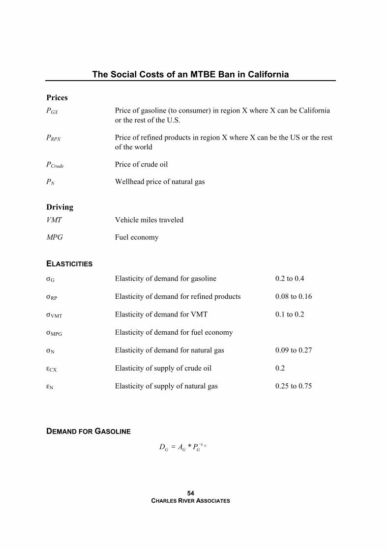
The Social Costs of an MTBE Ban in California
54 CHARLES RIVER ASSOCIATES
Prices
PGX Price of gasoline (to consumer) in region X where X can be California or the rest of the U.S.
PRPX Price of refined products in region X where X can be the US or the rest of the world
PCrude Price of crude oil
PN Wellhead price of natural gas
Driving
VMT Vehicle miles traveled
MPG Fuel economy
ELASTICITIES
σG Elasticity of demand for gasoline 0.2 to 0.4
σRP Elasticity of demand for refined products 0.08 to 0.16
σVMT Elasticity of demand for VMT 0.1 to 0.2
σMPG Elasticity of demand for fuel economy
σN Elasticity of demand for natural gas 0.09 to 0.27
εCX Elasticity of supply of crude oil 0.2
εN Elasticity of supply of natural gas 0.25 to 0.75
DEMAND FOR GASOLINE
GGGG PAD σ−= *
The Social Costs of an MTBE Ban in California
55 CHARLES RIVER ASSOCIATES
Gasoline demand is the product of two variables, miles driven (VMT) and gallons consumed per mile (1/MPG). Consumers make short run decisions about driving in response to fuel prices (car pooling, vacation trips, weekend travel, discretionary shopping) and in the long run the fuel economy of new cars, and ultimately the fleet, reflects a balancing of the costs of introducing fuel saving technologies and changes in the mix of vehicles toward smaller and more fuel efficient models, against the resulting savings in fuel consumption. VMT falls in response to higher gasoline prices and fuel economy (expressed in mpg) increases in response to higher gasoline prices, so that the two elasticities of demand are opposite in sign. Therefore, we can express
G VMT MPGσ σ σ= −
We distinguish between demand for gasoline in California DGCal and demand for gasoline in the rest of the US, DGXCal. Demand for other refined products is denoted DRPUS and total demand for petroleum products in the U.S. is DGCal + DGXCal + DRPUS. We denote demand for refined products outside the US as DRPNUS.
In general, demand for gasoline and refined products is a function of the world oil price plus the appropriate refiners margin, written as Pcrude + RMproduct, region. For simplicity, RMproduct,
region is assumed to be fixed, equivalent to assuming constant marginal refining costs.
EFFECTS OF MTBE ON GASOLINE DEMAND IN CALIFORNIA
The increase in refining cost, including the value of lost fuel economy, increases the price of gasoline in California. The per-gallon cost of producing a replacement for MTBE is added to the refiner’s margin for gasoline in California. We include the calculated value of the loss in fuel economy in the cost of producing the MTBE replacement.
The quantity of gasoline demand in California is shifted outward by the two additive factors of the net loss in volume due to removal of MTBE and the reduction in fuel economy. We define MTBEShift to be the sum of the effects of replacing MTBE volume and the change in fuel economy. It is calculated by multiplying the percentage loss of volume and change in fuel economy by baseline gasoline consumption in California. Thus, in the MTBE ban, the demand for gasoline in California is represented by
( )GCal CrudeMTBEBan GcalMTBEBanD p RM MTBEShift+ +
where RMGcalMTBEBan = RM0 + Fuelcst equals the absolute increase in cost of refining plus the value of lost fuel economy.
The Social Costs of an MTBE Ban in California
56 CHARLES RIVER ASSOCIATES
WORLD OIL MARKET
The supply of crude oil in the U.S. is SCUS and supply of crude oil in the rest of the world is SCXUS. Crude supply is a function of the price of crude oil, Pcrude.
The market clearing equilibrium condition that must be satisfied by Pcrude is
DGCal + DGXCal + DRPUS + DRPNUS = SCUS + SCXUS.
The model is benchmarked to year 2000 forecasts from the EIA Annual Energy Outlook 2001, and then solved with the shifts in demand and supply associated with the MTBE ban to estimate impacts of the demand on supply, demand and prices.
NATURAL GAS SUPPLY AND DEMAND
NNNN PAD σ−= *
* NN N NS B P ε=
Natural gas supply is a function of the wellhead price of natural gas, PN. The market clearing equilibrium that must be satisfied by PN is:
DNUS + DNCanada = SNUS + SNCanada
The Social Costs of an MTBE Ban in California
57 CHARLES RIVER ASSOCIATES
DATA
The following table provides the data used to benchmark the oil supply and demand model, elasticity assumptions, and values for MTBE ban costs and shift factors.
2000 Data
U.S. Natural Gas
Demand 22.24 Tcf
Production 18.72 Tcf
Imports 3.51 Tcf
Canada Natural Gas
Demand 3.1 Tcf
Production 6.61 Tcf
Crude Oil Production
U.S. 9.16 mmbd
Rest of World 67.48 mmbd
Demand for Refined Products
California Gasoline 14,490 mgal/year
Rest of U.S. Gasoline 114,895 mgal/year
Other U.S. Refined Products 11.05 mmbd.
Rest of World Refined Products 56.50 mmbd.
World Oil Supply 76.65 mmbd
U.S. Oil Consumption 19.48 mmbd
Prices
California Gasoline 1.64 $/gal
World Oil Price 27.59 $/bbl
Natural Gas Wellhead Price 3.28 $/mmbtu
Sources: EIA AEO 2001, NPC 1999
Ethanol Non-Oxy
Refiner Cost ($/gallon) 0.055 0.049
Change in Fuel Economy -0.4% 0.8%
Petroleum Volume Offset 5.8% 11.5%
Natural Gas Volume Increase 11.5% 11.5%
The Social Costs of an MTBE Ban in California
58 CHARLES RIVER ASSOCIATES
ESTIMATION OF CONSUMER SURPLUS LOSS
Consumer surplus in the California gasoline market
The MTBE ban causes the following impacts to the effective price of California gasoline:
1. An additive increase in the refiner’s margin equal to the change in refining cost (including the fuel economy penalty)
2. An additive increase in the price of gasoline equal to the increase in the world crude oil price
These changes alter the limits of integration used for calculating consumer surplus. The change in fuel economy alters gasoline consumption, but we assume that welfare is proportional to driving, not gasoline consumption, and do not include any welfare gain from the greater gasoline consumption required to provide the same VMT after the MTBE ban.
Consumer surplus in other products
Consumer surplus in other refined product markets, including gasoline consumed in the rest of the country and all other refined products, is affected only by the change in the world crude oil price.
Cost of producing crude oil
The increase in real resource cost of producing crude oil domestically is determined by the increase in the world crude oil price.
Cost of oil imports
The real resource cost of increased oil imports is the increase in the world oil price times the equilibrium quantity of imports after the MTBE ban. Other costs of increased oil imports are accounted for in consumer surplus losses in refined product consumption and cost increases in crude oil production attributable to higher oil prices.
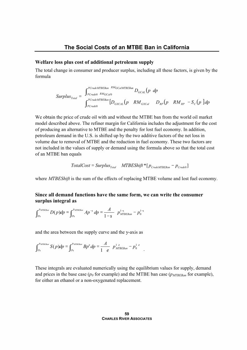
The Social Costs of an MTBE Ban in California
59 CHARLES RIVER ASSOCIATES
Welfare loss plus cost of additional petroleum supply
The total change in consumer and producer surplus, including all these factors, is given by the formula
( )
( ) ( ) ( )[ ]dppSRMpDRMpD
dppDSurplus
anCrudeMTBEBp
Crudep CRPRPGXCalGXCAL
nGCalMTBEBaRManCrudeMTBEBp
GCalRMCrudep GCAL
Total
∫
∫−+++
+=
+
+
0
00
We obtain the price of crude oil with and without the MTBE ban from the world oil market model described above. The refiner margin for California includes the adjustment for the cost of producing an alternative to MTBE and the penalty for lost fuel economy. In addition, petroleum demand in the U.S. is shifted up by the two additive factors of the net loss in volume due to removal of MTBE and the reduction in fuel economy. These two factors are not included in the values of supply or demand using the formula above so that the total cost of an MTBE ban equals
0[ ]Total CrudeMTBEBan CrudeTotalCost Surplus MTBEShift p p= + ∗ −
where MTBEShift is the sum of the effects of replacing MTBE volume and lost fuel economy.
Since all demand functions have the same form, we can write the consumer surplus integral as
0 0
1 10( )
1MTBEBan MTBEBanp p
MTBEBanp p
AD p dp Ap dp p pσ σ σ
σ− − − = = − −∫ ∫
and the area between the supply curve and the y-axis as
0 0
1 10( )
1MTBEBan MTBEBanp p
MTBEBanp p
AS p dp Bp dp p pε ε ε
ε+ + = = − +∫ ∫ .
These integrals are evaluated numerically using the equilibrium values for supply, demand and prices in the base case (p0 for example) and the MTBE ban case (pMTBEBan for example), for either an ethanol or a non-oxygenated replacement.
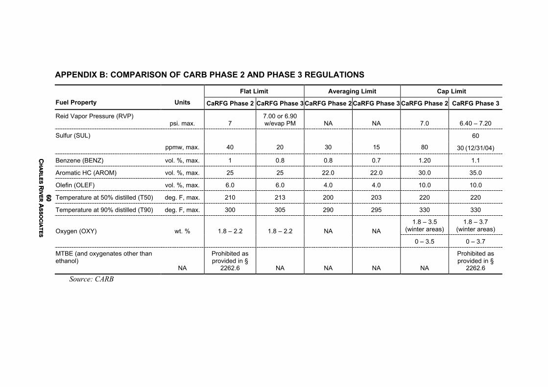
60C
HA
RL
ES
RIV
ER
AS
SO
CIA
TE
S60
CH
AR
LE
S R
IVE
R A
SS
OC
IAT
ES
APPENDIX B: COMPARISON OF CARB PHASE 2 AND PHASE 3 REGULATIONS
Flat Limit Averaging Limit Cap Limit Fuel Property
Units CaRFG Phase 2 CaRFG Phase 3 CaRFG Phase 2 CaRFG Phase 3 CaRFG Phase 2 CaRFG Phase 3
Reid Vapor Pressure (RVP) psi. max. 7
7.00 or 6.90 w/evap PM NA NA 7.0 6.40 – 7.20
60 Sulfur (SUL)
ppmw, max. 40 20 30 15 80 30 (12/31/04)
Benzene (BENZ) vol. %, max. 1 0.8 0.8 0.7 1.20 1.1
Aromatic HC (AROM) vol. %, max. 25 25 22.0 22.0 30.0 35.0
Olefin (OLEF) vol. %, max. 6.0 6.0 4.0 4.0 10.0 10.0
Temperature at 50% distilled (T50) deg. F, max. 210 213 200 203 220 220
Temperature at 90% distilled (T90) deg. F, max. 300 305 290 295 330 330
1.8 – 3.5 (winter areas)
1.8 – 3.7 (winter areas) Oxygen (OXY) wt. % 1.8 – 2.2 1.8 – 2.2 NA NA
0 – 3.5 0 – 3.7
MTBE (and oxygenates other than ethanol)
NA
Prohibited as provided in §
2262.6 NA NA NA NA
Prohibited as provided in §
2262.6
Source: CARB
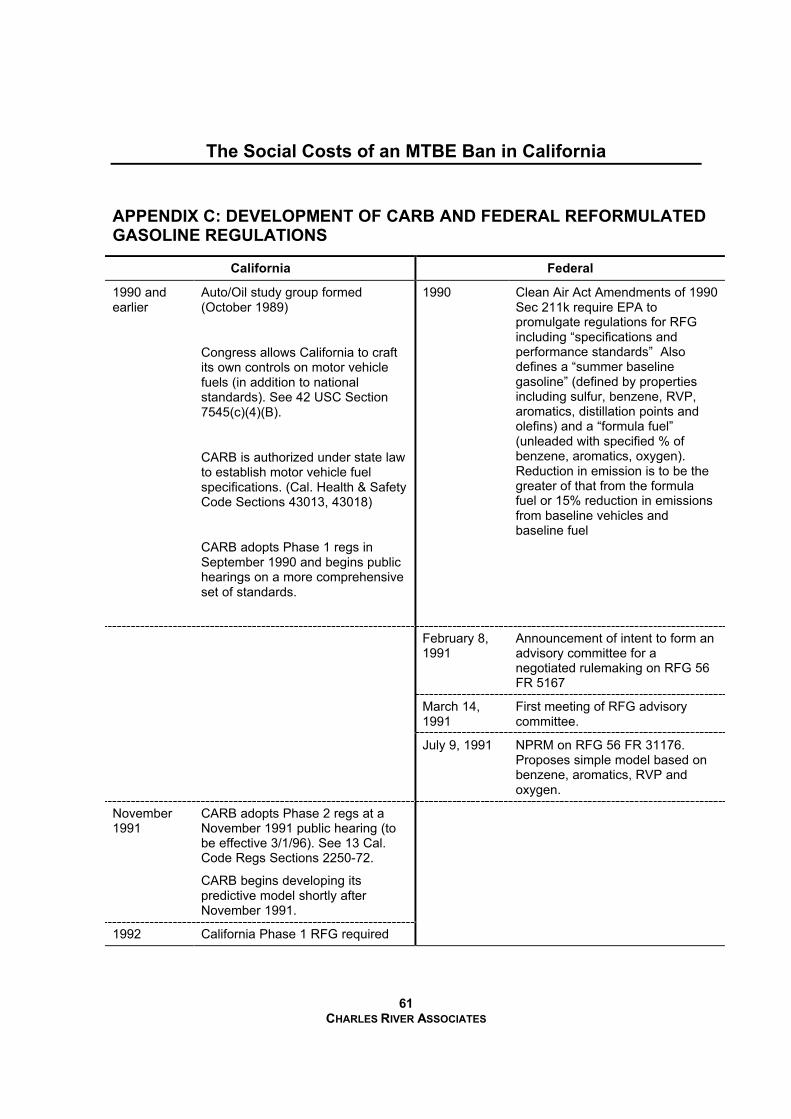
The Social Costs of an MTBE Ban in California
61 CHARLES RIVER ASSOCIATES
APPENDIX C: DEVELOPMENT OF CARB AND FEDERAL REFORMULATED GASOLINE REGULATIONS
California Federal
1990 and earlier
Auto/Oil study group formed (October 1989)
Congress allows California to craft its own controls on motor vehicle fuels (in addition to national standards). See 42 USC Section 7545(c)(4)(B).
CARB is authorized under state law to establish motor vehicle fuel specifications. (Cal. Health & Safety Code Sections 43013, 43018)
CARB adopts Phase 1 regs in September 1990 and begins public hearings on a more comprehensive set of standards.
1990 Clean Air Act Amendments of 1990 Sec 211k require EPA to promulgate regulations for RFG including “specifications and performance standards” Also defines a “summer baseline gasoline” (defined by properties including sulfur, benzene, RVP, aromatics, distillation points and olefins) and a “formula fuel” (unleaded with specified % of benzene, aromatics, oxygen). Reduction in emission is to be the greater of that from the formula fuel or 15% reduction in emissions from baseline vehicles and baseline fuel
February 8, 1991
Announcement of intent to form an advisory committee for a negotiated rulemaking on RFG 56 FR 5167
March 14, 1991
First meeting of RFG advisory committee.
July 9, 1991 NPRM on RFG 56 FR 31176. Proposes simple model based on benzene, aromatics, RVP and oxygen.
November 1991
CARB adopts Phase 2 regs at a November 1991 public hearing (to be effective 3/1/96). See 13 Cal. Code Regs Sections 2250-72.
CARB begins developing its predictive model shortly after November 1991.
1992 California Phase 1 RFG required
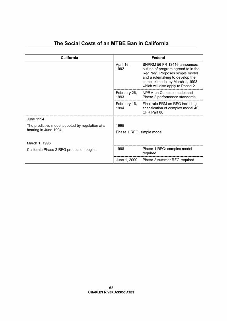
The Social Costs of an MTBE Ban in California
62 CHARLES RIVER ASSOCIATES
California Federal
April 16, 1992
SNPRM 56 FR 13416 announces outline of program agreed to in the Reg Neg. Proposes simple model and a rulemaking to develop the complex model by March 1, 1993 which will also apply to Phase 2.
February 26, 1993
NPRM on Complex model and Phase 2 performance standards.
February 16, 1994
Final rule FRM on RFG including specification of complex model 40 CFR Part 80
June 1994
The predictive model adopted by regulation at a hearing in June 1994.
1995
Phase 1 RFG: simple model
1998 Phase 1 RFG: complex model required
March 1, 1996
California Phase 2 RFG production begins
June 1, 2000 Phase 2 summer RFG required
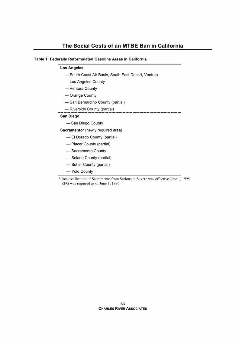
The Social Costs of an MTBE Ban in California
63 CHARLES RIVER ASSOCIATES
Table 1: Federally Reformulated Gasoline Areas in California
Los Angeles
— South Coast Air Basin, South East Desert, Ventura
— Los Angeles County
— Ventura County
— Orange County
— San Bernardino County (partial)
— Riverside County (partial)
San Diego
— San Diego County
Sacramento* (newly required area)
— El Dorado County (partial)
— Placer County (partial)
— Sacramento County
— Solano County (partial)
— Sutter County (partial)
— Yolo County
* Reclassification of Sacramento from Serious to Severe was effective June 1, 1995. RFG was required as of June 1, 1996.
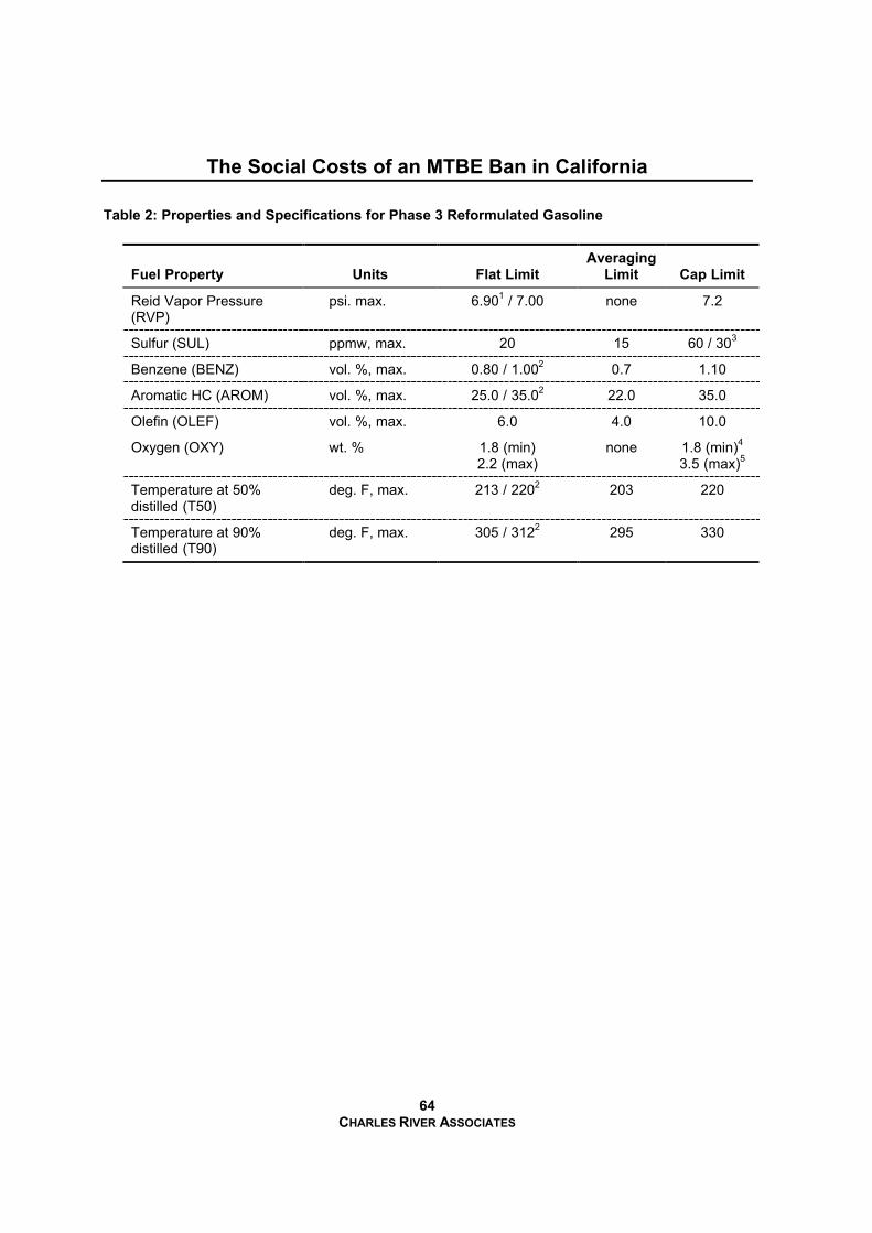
The Social Costs of an MTBE Ban in California
64 CHARLES RIVER ASSOCIATES
Table 2: Properties and Specifications for Phase 3 Reformulated Gasoline
Fuel Property
Units
Flat Limit
Averaging Limit
Cap Limit
Reid Vapor Pressure (RVP)
psi. max. 6.901 / 7.00 none 7.2
Sulfur (SUL) ppmw, max. 20 15 60 / 303
Benzene (BENZ) vol. %, max. 0.80 / 1.002 0.7 1.10
Aromatic HC (AROM) vol. %, max. 25.0 / 35.02 22.0 35.0
Olefin (OLEF) vol. %, max. 6.0 4.0 10.0
Oxygen (OXY) wt. % 1.8 (min) 2.2 (max)
none 1.8 (min)4 3.5 (max)5
Temperature at 50% distilled (T50)
deg. F, max. 213 / 2202 203 220
Temperature at 90% distilled (T90)
deg. F, max. 305 / 3122 295 330
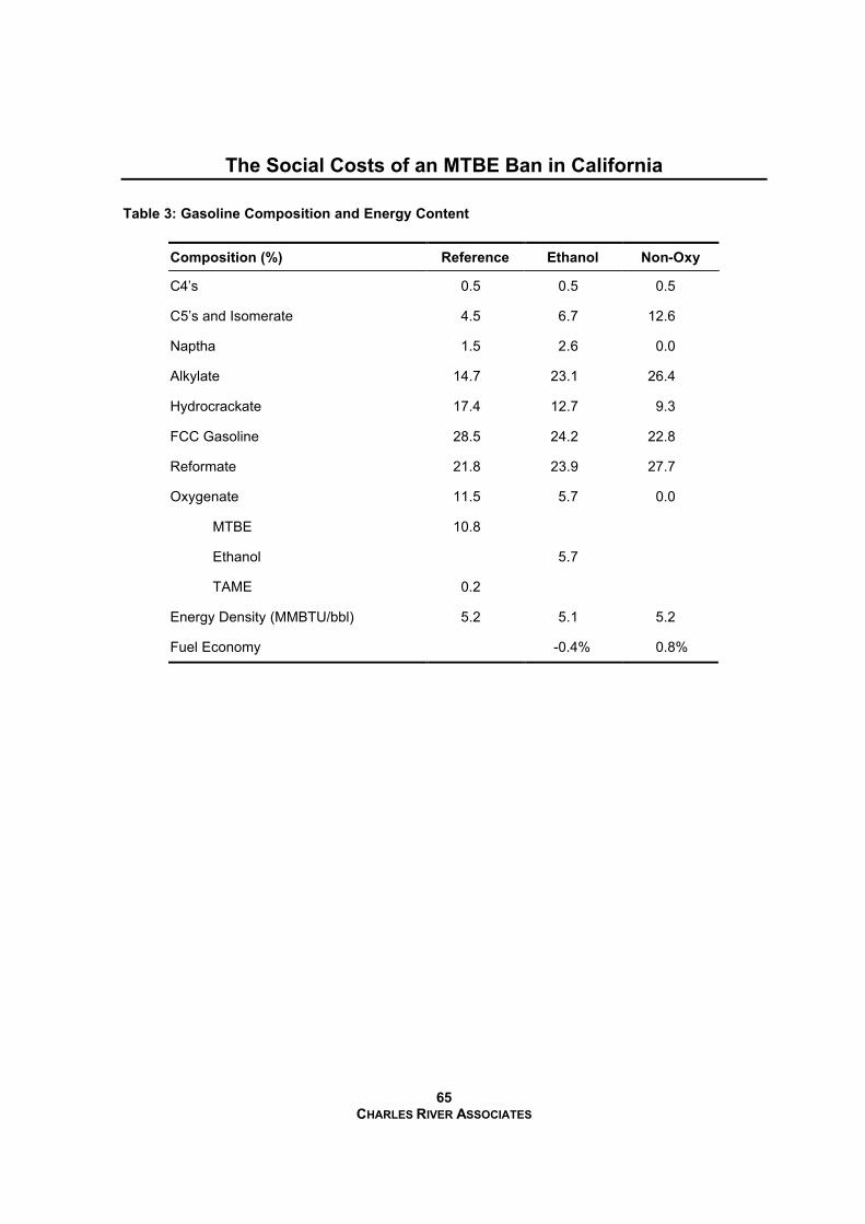
The Social Costs of an MTBE Ban in California
65 CHARLES RIVER ASSOCIATES
Table 3: Gasoline Composition and Energy Content
Composition (%) Reference Ethanol Non-Oxy
C4’s 0.5 0.5 0.5
C5’s and Isomerate 4.5 6.7 12.6
Naptha 1.5 2.6 0.0
Alkylate 14.7 23.1 26.4
Hydrocrackate 17.4 12.7 9.3
FCC Gasoline 28.5 24.2 22.8
Reformate 21.8 23.9 27.7
Oxygenate 11.5 5.7 0.0
MTBE 10.8
Ethanol 5.7
TAME 0.2
Energy Density (MMBTU/bbl) 5.2 5.1 5.2
Fuel Economy -0.4% 0.8%
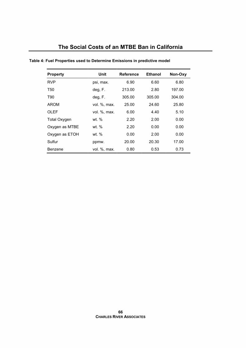
The Social Costs of an MTBE Ban in California
66 CHARLES RIVER ASSOCIATES
Table 4: Fuel Properties used to Determine Emissions in predictive model
Property Unit Reference Ethanol Non-Oxy
RVP psi, max. 6.90 6.60 6.80
T50 deg, F. 213.00 2.80 197.00
T90 deg, F. 305.00 305.00 304.00
AROM vol. %, max. 25.00 24.60 25.80
OLEF vol. %, max. 6.00 4.40 5.10
Total Oxygen wt. % 2.20 2.00 0.00
Oxygen as MTBE wt. % 2.20 0.00 0.00
Oxygen as ETOH wt. % 0.00 2.00 0.00
Sulfur ppmw. 20.00 20.30 17.00
Benzene vol. %, max. 0.80 0.53 0.73
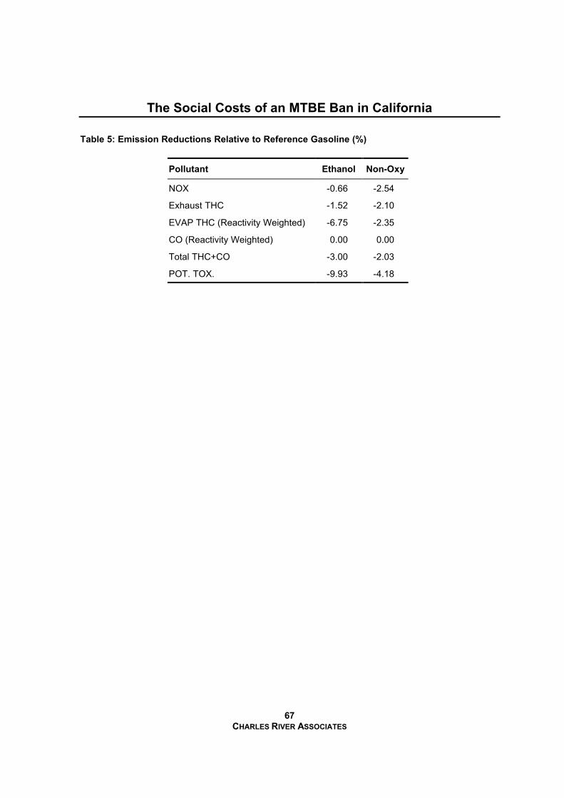
The Social Costs of an MTBE Ban in California
67 CHARLES RIVER ASSOCIATES
Table 5: Emission Reductions Relative to Reference Gasoline (%)
Pollutant Ethanol Non-Oxy
NOX -0.66 -2.54
Exhaust THC -1.52 -2.10
EVAP THC (Reactivity Weighted) -6.75 -2.35
CO (Reactivity Weighted) 0.00 0.00
Total THC+CO -3.00 -2.03
POT. TOX. -9.93 -4.18
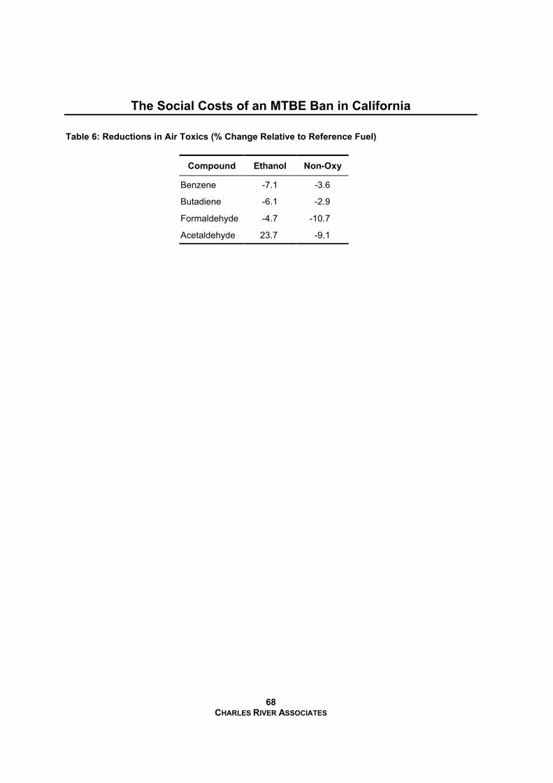
The Social Costs of an MTBE Ban in California
68 CHARLES RIVER ASSOCIATES
Table 6: Reductions in Air Toxics (% Change Relative to Reference Fuel)
Compound Ethanol Non-Oxy
Benzene -7.1 -3.6
Butadiene -6.1 -2.9
Formaldehyde -4.7 -10.7
Acetaldehyde 23.7 -9.1
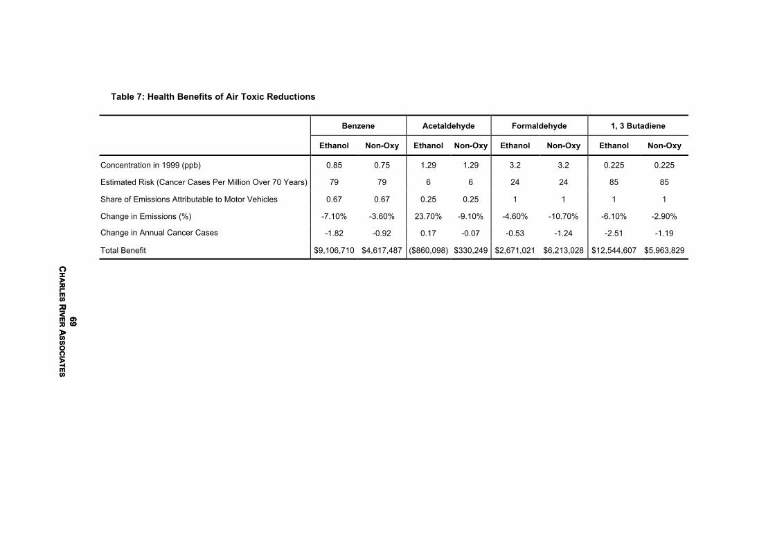
69C
HA
RL
ES
RIV
ER
AS
SO
CIA
TE
S69
CH
AR
LE
S R
IVE
R A
SS
OC
IAT
ES
Table 7: Health Benefits of Air Toxic Reductions
Benzene Acetaldehyde Formaldehyde 1, 3 Butadiene
Ethanol Non-Oxy Ethanol Non-Oxy Ethanol Non-Oxy Ethanol Non-Oxy
Concentration in 1999 (ppb) 0.85 0.75 1.29 1.29 3.2 3.2 0.225 0.225
Estimated Risk (Cancer Cases Per Million Over 70 Years) 79 79 6 6 24 24 85 85
Share of Emissions Attributable to Motor Vehicles 0.67 0.67 0.25 0.25 1 1 1 1
Change in Emissions (%) -7.10% -3.60% 23.70% -9.10% -4.60% -10.70% -6.10% -2.90%
Change in Annual Cancer Cases -1.82 -0.92 0.17 -0.07 -0.53 -1.24 -2.51 -1.19
Total Benefit $9,106,710 $4,617,487 ($860,098) $330,249 $2,671,021 $6,213,028 $12,544,607 $5,963,829
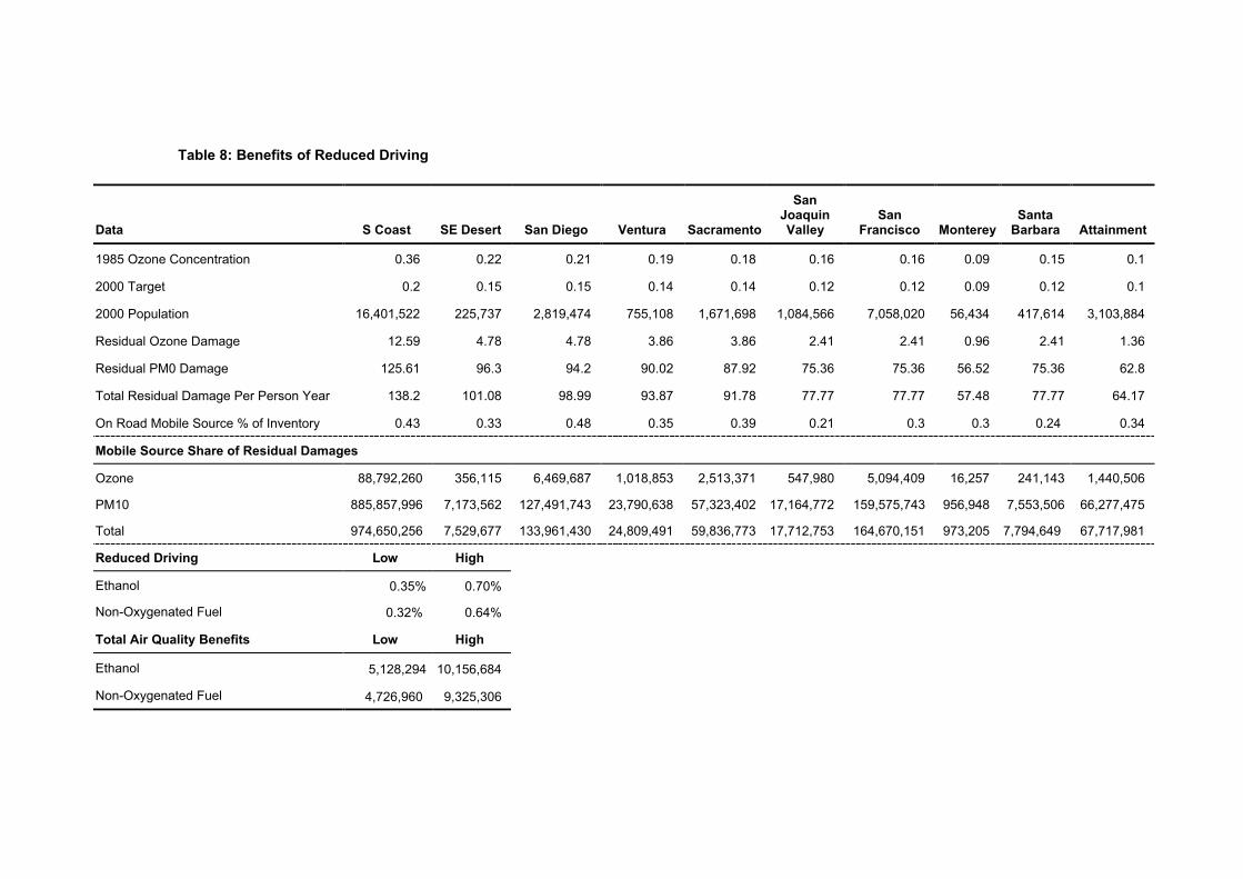
Table 8: Benefits of Reduced Driving
Data
S Coast
SE Desert
San Diego
Ventura
Sacramento
San Joaquin Valley
San
Francisco
Monterey
Santa
Barbara
Attainment
1985 Ozone Concentration 0.36 0.22 0.21 0.19 0.18 0.16 0.16 0.09 0.15 0.1
2000 Target 0.2 0.15 0.15 0.14 0.14 0.12 0.12 0.09 0.12 0.1
2000 Population 16,401,522 225,737 2,819,474 755,108 1,671,698 1,084,566 7,058,020 56,434 417,614 3,103,884
Residual Ozone Damage 12.59 4.78 4.78 3.86 3.86 2.41 2.41 0.96 2.41 1.36
Residual PM0 Damage 125.61 96.3 94.2 90.02 87.92 75.36 75.36 56.52 75.36 62.8
Total Residual Damage Per Person Year 138.2 101.08 98.99 93.87 91.78 77.77 77.77 57.48 77.77 64.17
On Road Mobile Source % of Inventory 0.43 0.33 0.48 0.35 0.39 0.21 0.3 0.3 0.24 0.34
Mobile Source Share of Residual Damages
Ozone 88,792,260 356,115 6,469,687 1,018,853 2,513,371 547,980 5,094,409 16,257 241,143 1,440,506
PM10 885,857,996 7,173,562 127,491,743 23,790,638 57,323,402 17,164,772 159,575,743 956,948 7,553,506 66,277,475
Total 974,650,256 7,529,677 133,961,430 24,809,491 59,836,773 17,712,753 164,670,151 973,205 7,794,649 67,717,981
Reduced Driving Low High
Ethanol 0.35% 0.70%
Non-Oxygenated Fuel 0.32% 0.64%
Total Air Quality Benefits Low High
Ethanol 5,128,294 10,156,684
Non-Oxygenated Fuel 4,726,960 9,325,306
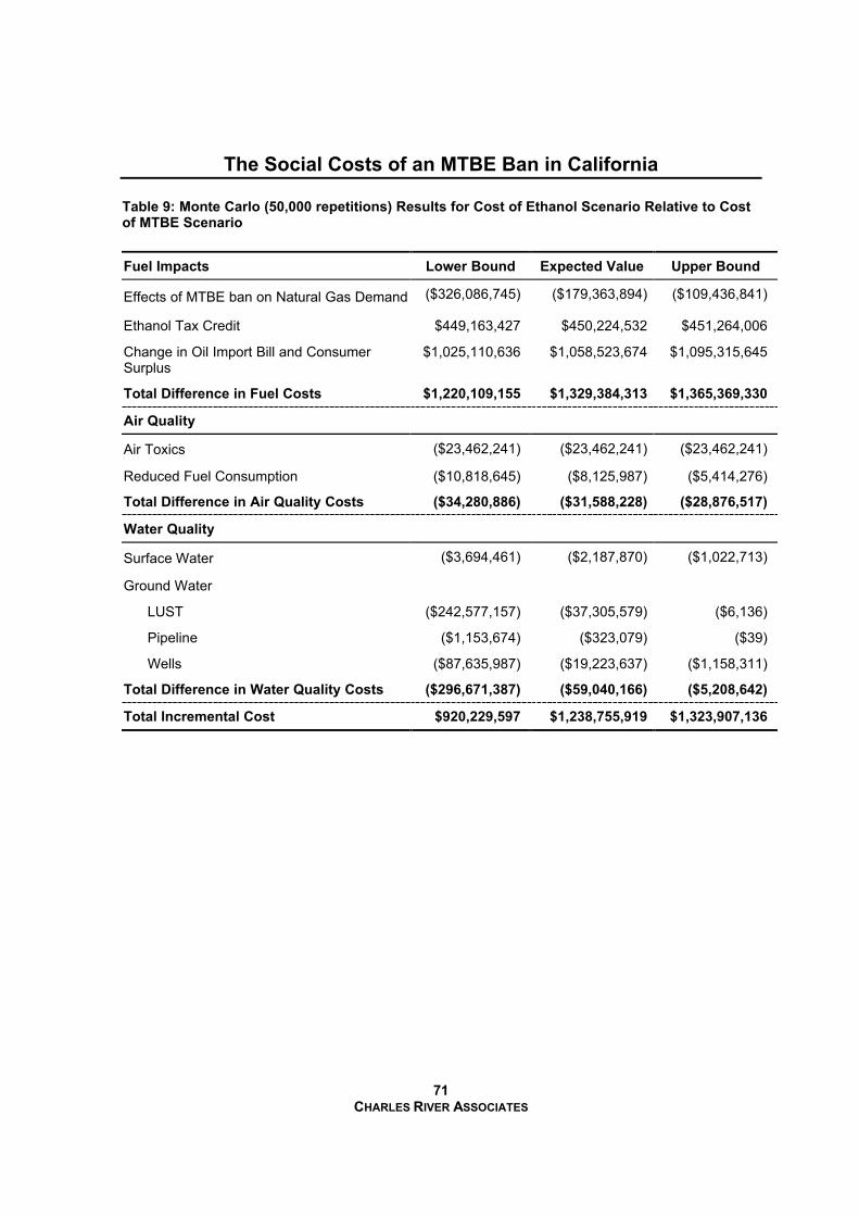
The Social Costs of an MTBE Ban in California
71 CHARLES RIVER ASSOCIATES
Table 9: Monte Carlo (50,000 repetitions) Results for Cost of Ethanol Scenario Relative to Cost of MTBE Scenario
Fuel Impacts Lower Bound Expected Value Upper Bound
Effects of MTBE ban on Natural Gas Demand ($326,086,745) ($179,363,894) ($109,436,841)
Ethanol Tax Credit $449,163,427 $450,224,532 $451,264,006
Change in Oil Import Bill and Consumer Surplus
$1,025,110,636 $1,058,523,674 $1,095,315,645
Total Difference in Fuel Costs $1,220,109,155 $1,329,384,313 $1,365,369,330
Air Quality
Air Toxics ($23,462,241) ($23,462,241) ($23,462,241)
Reduced Fuel Consumption ($10,818,645) ($8,125,987) ($5,414,276)
Total Difference in Air Quality Costs ($34,280,886) ($31,588,228) ($28,876,517)
Water Quality
Surface Water ($3,694,461) ($2,187,870) ($1,022,713)
Ground Water
LUST ($242,577,157) ($37,305,579) ($6,136)
Pipeline ($1,153,674) ($323,079) ($39)
Wells ($87,635,987) ($19,223,637) ($1,158,311)
Total Difference in Water Quality Costs ($296,671,387) ($59,040,166) ($5,208,642)
Total Incremental Cost $920,229,597 $1,238,755,919 $1,323,907,136
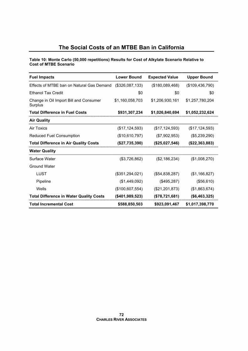
The Social Costs of an MTBE Ban in California
72 CHARLES RIVER ASSOCIATES
Table 10: Monte Carlo (50,000 repetitions) Results for Cost of Alkylate Scenario Relative to Cost of MTBE Scenario
Fuel Impacts Lower Bound Expected Value Upper Bound
Effects of MTBE ban on Natural Gas Demand ($326,087,133) ($180,089,468) ($109,436,790)
Ethanol Tax Credit $0 $0 $0
Change in Oil Import Bill and Consumer Surplus
$1,160,058,703 $1,206,930,161 $1,257,780,204
Total Difference in Fuel Costs $931,307,234 $1,026,840,694 $1,052,232,624
Air Quality
Air Toxics ($17,124,593) ($17,124,593) ($17,124,593)
Reduced Fuel Consumption ($10,610,797) ($7,902,953) ($5,239,290)
Total Difference in Air Quality Costs ($27,735,390) ($25,027,546) ($22,363,883)
Water Quality
Surface Water ($3,726,862) ($2,186,234) ($1,008,270)
Ground Water
LUST ($351,294,021) ($54,838,287) ($1,166,827)
Pipeline ($1,449,092) ($495,287) ($56,610)
Wells ($100,607,554) ($21,201,873) ($1,863,674)
Total Difference in Water Quality Costs ($401,989,523) ($78,721,681) ($6,463,325)
Total Incremental Cost $588,850,503 $923,091,467 $1,017,398,770
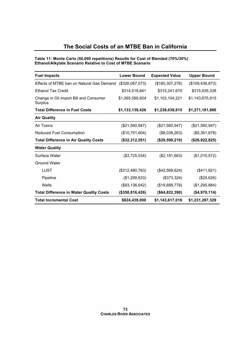
The Social Costs of an MTBE Ban in California
73 CHARLES RIVER ASSOCIATES
Table 11: Monte Carlo (50,000 repetitions) Results for Cost of Blended (70%/30%) Ethanol/Alkylate Scenario Relative to Cost of MTBE Scenario
Fuel Impacts Lower Bound Expected Value Upper Bound
Effects of MTBE ban on Natural Gas Demand ($326,087,073) ($180,307,276) ($109,436,873)
Ethanol Tax Credit $314,518,841 $315,241,670 $315,935,338
Change in Oil Import Bill and Consumer Surplus
$1,065,590,924 $1,103,104,221 $1,143,675,915
Total Difference in Fuel Costs $1,133,139,426 $1,238,038,615 $1,271,181,886
Air Quality
Air Toxics ($21,560,947) ($21,560,947) ($21,560,947)
Reduced Fuel Consumption ($10,751,604) ($8,038,263) ($5,361,878)
Total Difference in Air Quality Costs ($32,312,551) ($29,599,210) ($26,922,825)
Water Quality
Surface Water ($3,725,534) ($2,191,663) ($1,010,572)
Ground Water
LUST ($312,480,763) ($42,568,624) ($411,821)
Pipeline ($1,299,833) ($373,324) ($25,626)
Wells ($93,136,642) ($19,688,778) ($1,295,884)
Total Difference in Water Quality Costs ($358,816,426) ($64,822,390) ($4,970,114)
Total Incremental Cost $824,439,000 $1,143,617,016 $1,231,287,329
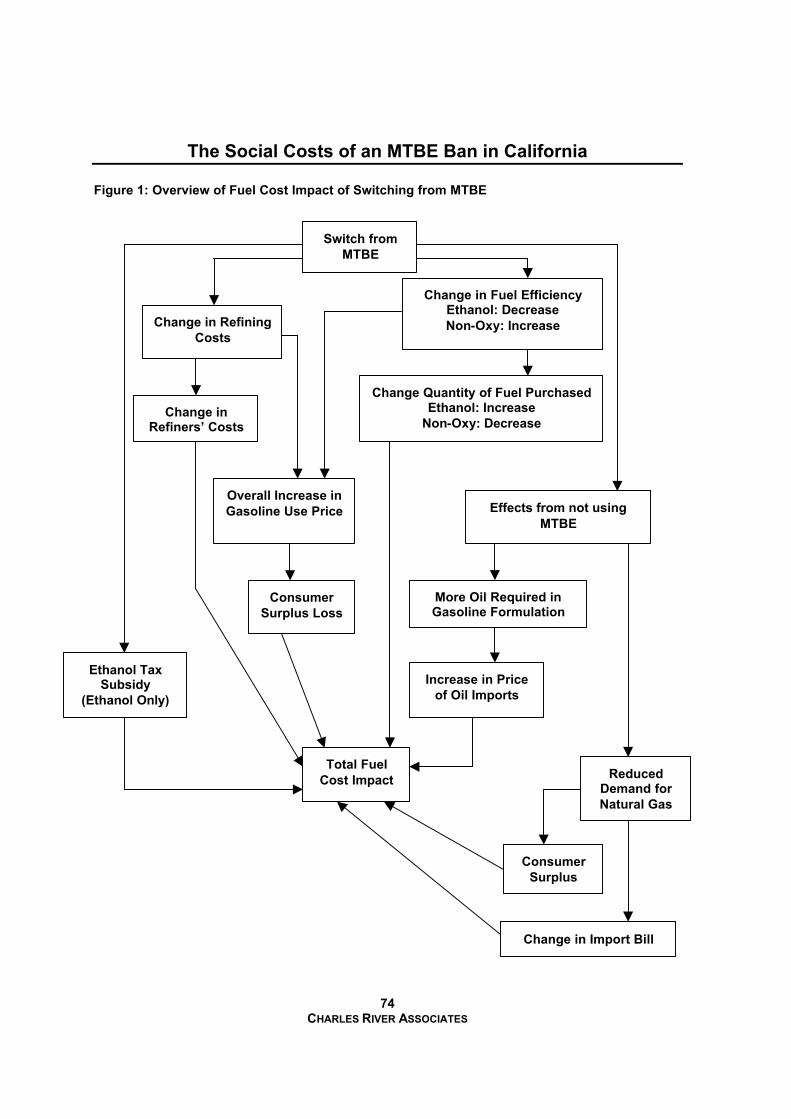
The Social Costs of an MTBE Ban in California
74 CHARLES RIVER ASSOCIATES
Figure 1: Overview of Fuel Cost Impact of Switching from MTBE
Change Quantity of Fuel Purchased Ethanol: Increase
Non-Oxy: Decrease
Change in Fuel Efficiency Ethanol: Decrease Non-Oxy: Increase
Total Fuel Cost Impact
Change in Refiners’ Costs
Change in Refining Costs
Switch from MTBE
Overall Increase in Gasoline Use Price
Consumer Surplus Loss
Ethanol Tax Subsidy
(Ethanol Only)
Effects from not using MTBE
More Oil Required in Gasoline Formulation
Consumer Surplus
Reduced Demand for Natural Gas
Change in Import Bill
Increase in Price of Oil Imports
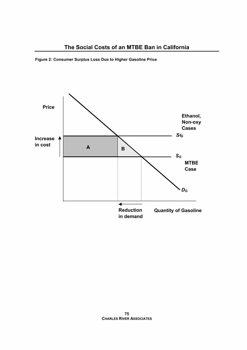
The Social Costs of an MTBE Ban in California
75 CHARLES RIVER ASSOCIATES
Figure 2: Consumer Surplus Loss Due to Higher Gasoline Price
A B
Quantity of Gasoline
Increase in cost
Reduction in demand
MTBE Case
Ethanol, Non-oxy Cases
Price
DG
SG
S′G
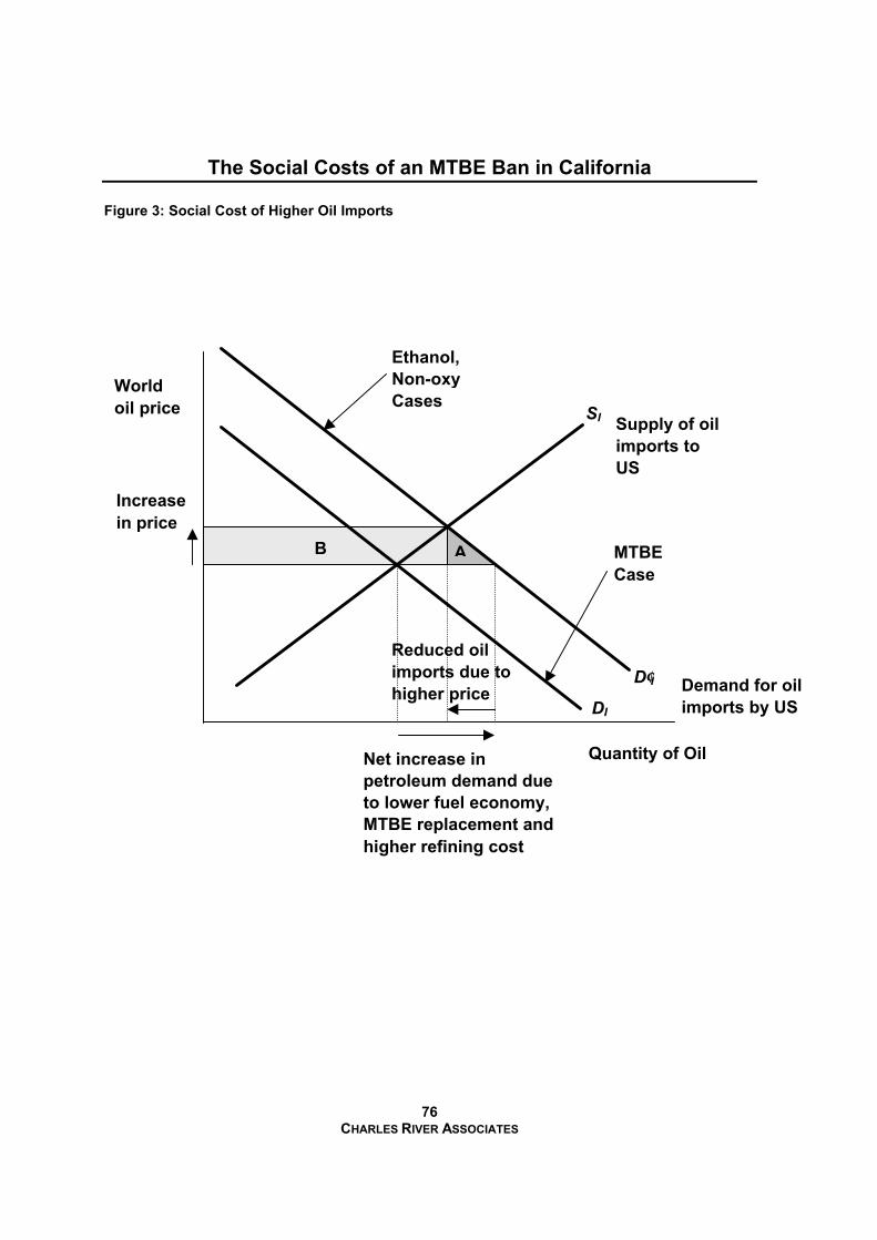
The Social Costs of an MTBE Ban in California
76 CHARLES RIVER ASSOCIATES
Figure 3: Social Cost of Higher Oil Imports
Quantity of Oil
Increase in price
Reduced oil imports due to higher price
MTBE Case
Ethanol, Non-oxy Cases
Net increase in petroleum demand due to lower fuel economy, MTBE replacement and higher refining cost
World oil price
Supply of oil imports to US
Demand for oil imports by US
B A
SI
D′I
DI
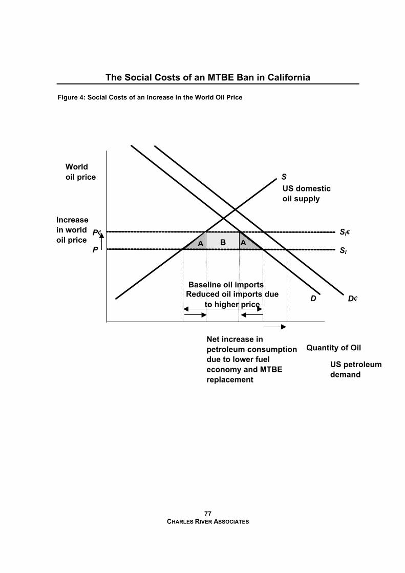
The Social Costs of an MTBE Ban in California
77 CHARLES RIVER ASSOCIATES
US petroleum demand
Figure 4: Social Costs of an Increase in the World Oil Price
Quantity of Oil
Increase in world oil price
Reduced oil imports due to higher price
Net increase in petroleum consumption due to lower fuel economy and MTBE replacement
World oil price
US domestic oil supply
B A P′
D
P A
D′
S
SI
SI′
Baseline oil imports
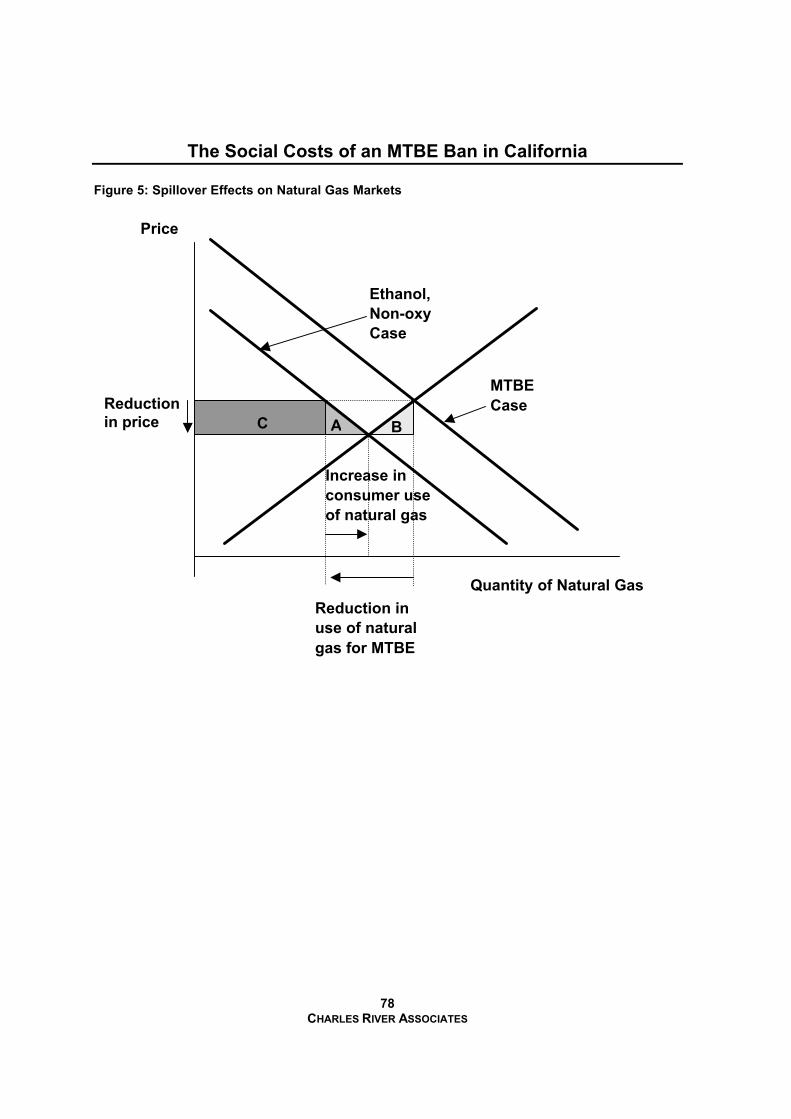
The Social Costs of an MTBE Ban in California
78 CHARLES RIVER ASSOCIATES
Figure 5: Spillover Effects on Natural Gas Markets
Price
Quantity of Natural Gas Reduction in use of natural gas for MTBE
A Reduction in price
MTBE Case
Ethanol, Non-oxy Case
Increase in consumer use of natural gas
B C
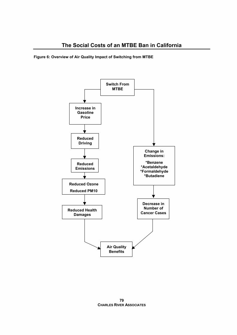
The Social Costs of an MTBE Ban in California
79 CHARLES RIVER ASSOCIATES
Figure 6: Overview of Air Quality Impact of Switching from MTBE
Increase in Gasoline
Price
Reduced Driving
Reduced Emissions
Reduced Ozone
Reduced PM10
Decrease in Number of
Cancer Cases
Switch From MTBE
Air Quality Benefits
Change in Emissions:
*Benzene *Acetaldehyde *Formaldehyde
*Butadiene
Reduced Health Damages
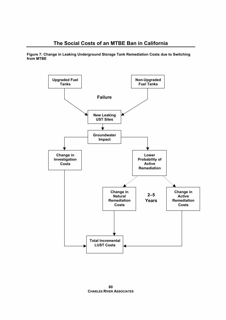
The Social Costs of an MTBE Ban in California
80 CHARLES RIVER ASSOCIATES
Figure 7: Change in Leaking Underground Storage Tank Remediation Costs due to Switching from MTBE
Upgraded Fuel Tanks
Change in Active
Remediation Costs
Change in Natural
Remediation Costs
Change in Investigation
Costs
Groundwater Impact
New Leaking UST Sites
Non-Upgraded Fuel Tanks
Failure
2–5 Years
Total Incremental LUST Costs
Lower Probability of
Active Remediation
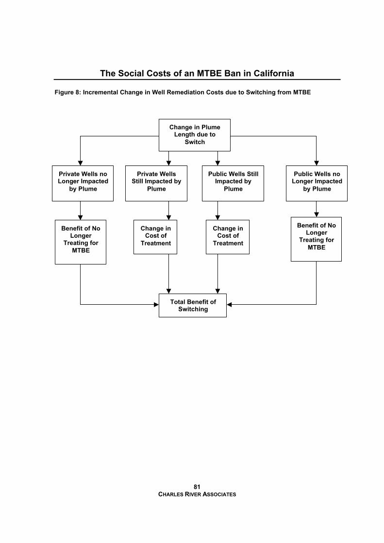
The Social Costs of an MTBE Ban in California
81 CHARLES RIVER ASSOCIATES
Figure 8: Incremental Change in Well Remediation Costs due to Switching from MTBE
Total Benefit of Switching
Change in Cost of
Treatment
Benefit of No Longer
Treating for MTBE
Change in Plume Length due to
Switch
Private Wells no Longer Impacted
by Plume
Public Wells no Longer Impacted
by Plume
Private Wells Still Impacted by
Plume
Public Wells Still Impacted by
Plume
Change in Cost of
Treatment
Benefit of No Longer
Treating for MTBE
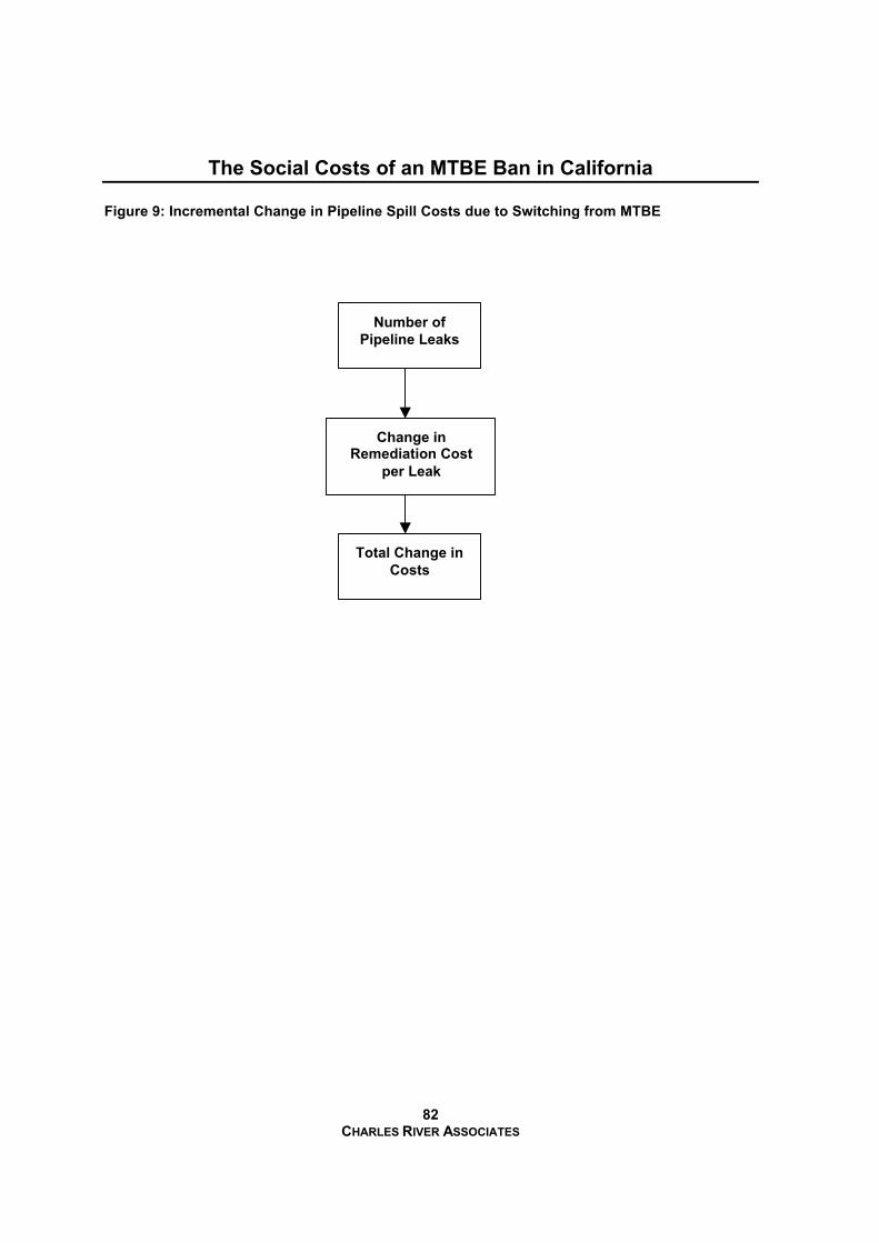
The Social Costs of an MTBE Ban in California
82 CHARLES RIVER ASSOCIATES
Figure 9: Incremental Change in Pipeline Spill Costs due to Switching from MTBE
Number of Pipeline Leaks
Change in Remediation Cost
per Leak
Total Change in Costs
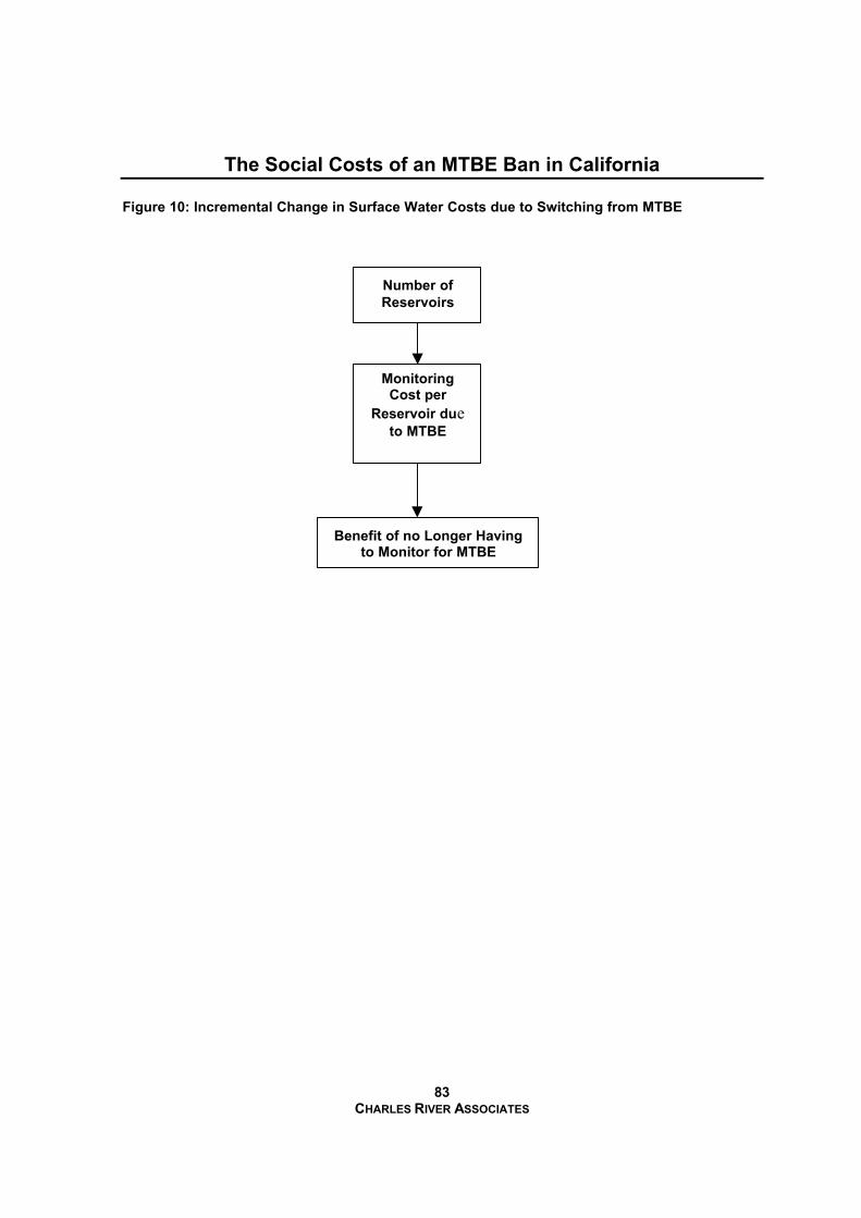
The Social Costs of an MTBE Ban in California
83 CHARLES RIVER ASSOCIATES
Figure 10: Incremental Change in Surface Water Costs due to Switching from MTBE
Number of Reservoirs
Monitoring Cost per
Reservoir due to MTBE
Benefit of no Longer Having to Monitor for MTBE