Physica A 397 (2014) 1–16

Contents lists available at ScienceDirect

Physica A

journal homepage: www.elsevier.com/locate/physa

The Sherrington–Kirkpatrick spin glass model in the presenceof a random field with a joint Gaussian probability densityfunction for the exchange interactions and random fieldsIoannis A. Hadjiagapiou ∗

Section of Solid State Physics, Department of Physics, University of Athens, Panepistimioupolis, GR 15784 Zografos, Athens, Greece

h i g h l i g h t s

• Sherrington–Kirkpatrick spin glass.• Replica trick.• Randommagnetic field.• Joint Gaussian probability density function.

a r t i c l e i n f o

Article history:Received 25 July 2013Received in revised form 30 October 2013Available online 9 December 2013

Keywords:Ising modelSpin glassFrustrationReplica methodRandom fieldGaussian probability density

a b s t r a c t

The magnetic systems with disorder form an important class of systems, which areunder intensive studies, since they reflect real systems. Such a class of systems is thespin glass one, which combines randomness and frustration. The Sherrington–KirkpatrickIsing spin glass with random couplings in the presence of a random magnetic field isinvestigated in detail within the framework of the replica method. The two randomvariables (exchange integral interaction and random magnetic field) are drawn from ajoint Gaussian probability density function characterized by a correlation coefficient ρ.The thermodynamic properties and phase diagrams are studied with respect to the naturalparameters of both random components of the system contained in the probability density.The de Almeida–Thouless line is explored as a function of temperature, ρ and other systemparameters. The entropy for zero temperature aswell as for non zero temperatures is partlynegative or positive, acquiring positive branches as h0 increases.

© 2013 Elsevier B.V. All rights reserved.

1. Introduction

The critical properties of magnetic systems with quenched disorder have been a topic of growing interest in statisticalphysics over the last years and still attracts considerable attention in spite of their long history, since it has been establishedthat the introduction of randomness can cause important effects on their thermodynamic behavior in comparison to the pureones; the type of the phase transition as well as the universality class may change [1–3]. In two-dimensions an infinitesimalamount of disorder converts a second-order phase transition (SOPT) into a first-order phase transition (FOPT), whereas inthree-dimensions it is converted to an FOPT onlywhen disorder exceeds a threshold. Randomness is encountered in the formof vacancies, variable or diluted bonds, impurities [4,5], random fields [6–13] and spin glasses [13–19]. In addition, the studyof disordered systems is a necessity because homogeneous systems are, in general, an idealization, whereas real materialscontain impurities, nonmagnetic atoms or vacancies randomly distributed within the system consisting of magnetic atoms,

∗ Tel.: +30 2107276771; fax: +30 2107276711.E-mail address: ihatziag@phys.uoa.gr.

0378-4371/$ – see front matter© 2013 Elsevier B.V. All rights reserved.http://dx.doi.org/10.1016/j.physa.2013.12.002

2 I.A. Hadjiagapiou / Physica A 397 (2014) 1–16

or variable bonds in magnitude and/or in sign; such systems have attracted wide interest and have been studied intensivelytheoretically, numerically and experimentally, since it is a matter of great urgency to develop an understanding of the roleof these non ideal effects. However, to facilitate their study, these are modeled by relying on pure-system models modifiedaccordingly, e.g. Ising, Potts, Baxter–Wu, etc.

An important manifestation of disorder is the presence of random magnetic fields acting on each spin of the magneticsystem under consideration in an otherwise free of defects lattice, whose pure version is modeled according to a currentone, e.g. the Ising model; the system now in the presence of such fields is called random field Ising model (RFIM) [6–13].Associatedwith this model are the notions of lower critical dimension, tricritical points, scaling laws, crossover phenomena,higher order critical points and random field probability distribution function (PDF). RFIM had been the standard vehicle forstudying the effects of quenched randomness on phase diagrams and critical properties of lattice spin systems and had beenstudied for many years since the seminal work of Imry andMa [11]. The RFIM Hamiltonian, in the case of constant exchangeintegral, is

H = −J⟨i,j⟩

SiSj −

i

hiSi, Si = ±1. (1)

This Hamiltonian describes the competition between the long-range order (expressed by the first summation) and therandom ordering fields. We also consider that J > 0 so that the ground state is ferromagnetic in absence of random fields.The RFIMmodel, despite its simple definition and apparent simplicity, together with the richness of the physical propertiesemerging from its study, hasmotivated a significant number of investigations; however, these properties have proved to be asource ofmuch controversy, primarily due to the lack of a reliable theoretical foundation. Still, substantial efforts to elucidatethe basic problems of the RFIM continue to attract considerable attention, because of its direct relevance to a number ofsignificant physical problems. The presence of random fields requires two averaging procedures, the usual thermal average,denoted by angular brackets ⟨. . .⟩, and disorder average over the random fields denoted by ⟨. . .⟩r for the respective PDF,which is usually a version of the bimodal, trimodal or Gaussian distributions. The most frequently used PDF for randomfields is either the bimodal or the single Gaussian; the former is,

P(hi) = pδ(hi − h0) + qδ(hi + h0) (2)

where p is the fraction of lattice sites having a magnetic field h0, while the rest sites have a field (−h0) with site probabilityq such that p + q = 1; the usual choice was p = q =

12 , symmetric case. The latter PDF is,

P(hi) =1

(2πσ 2)1/2exp

−

h2i

2σ 2

(3)

with zero mean and standard deviation σ .One of the main issues was the experimental realization of random fields. Fishman and Aharony [20] showed that the

randomly quenched exchange interactions Ising antiferromagnet in a uniform field H are equivalent to a ferromagnet in arandom field with the strength of the random field linearly proportional to the induced magnetization. This identificationgave new impetus to the study of the RFIM, the investigation gained further interest and was intensified resulting in a largenumber of publications (theoretical, numerical, Monte Carlo simulations and experimental) in the last thirty years. Althoughmuch effort had been invested towards this direction, the only well-established conclusion drawn was the existence ofa phase transition for d ≥ 3 (d space dimension), that is, the critical lower dimension dl is 2 after a long controversialdiscussion [11,21], while many other issues are still unanswered; among them is the order of the phase transition (firstor second order), the universality class and the dependence of these points on the form of the random field PDF. Galam,via MFA, has shown that the Ising antiferromagnets in a uniform field with either a general random site exchange or sitedilution have the same multicritical space as the random-field Ising model with bimodal PDF [22]. The study of RFIM hasalso highlighted another feature of the model, that of tricriticality and its dependence on the assumed distribution functionof the random fields. A very controversial issue has arisen concerning the effect of the random-field probability distributionfunction on the equilibrium phase diagram of the RFIM. The choice of the random field distribution can lead to a continuousferromagnetic/paramagnetic (FM/PM) boundary as in the single Gaussian PDF, whereas for the bimodal one this boundaryis divided into two parts, an SOPT branch for high temperatures and an FOPT branch for low temperatures separated bya tricritical point (TCP) at kT t

c /(zJ) = 2/3 and htc/(zJ) = (kT t

c /(zJ)) × arg tanh(1/√3) ≃ 0.439 [12], where z is the

coordination number and k is the Boltzmann constant, such that for T < T tc and h > ht

c the transition to the FM phase is offirst order for p =

12 . However, this behavior is not fully elucidated since in the case of the three-dimensional RFIM, the high

temperature series expansions by Gofman et al. [23] yielded only continuous transitions for both probability distributions,whereas according to Houghton et al. [24] both distributions predicted the existence of a TCP, with ht

c = 0.28 ± 0.01 andT tc = 0.49 ± 0.03 for the bimodal and σ t

c = 0.36 ± 0.01 and T tc = 0.36 ± 0.04 for the single Gaussian. In the Monte Carlo

studies for d = 3, Machta et al. [25], using single Gaussian distribution, could not reach a definite conclusion concerning thenature of the transition, since for some realizations of randomness the magnetization histogramwas two-peaked (implyingan SOPT) whereas for other ones three-peaked, implying an FOPT; Middleton and Fisher [26], using a similar distributionfor T = 0, suggested an SOPT with a small order parameter exponent β = 0.017(5). Malakis and Fytas [27], by applying the

I.A. Hadjiagapiou / Physica A 397 (2014) 1–16 3

critical minimum-energy subspace scheme in conjunction with the Wang–Landau and broad-histogram methods for cubiclattices, proved that the specific heat and susceptibility are non-self-averaging using the bimodal distribution.

Another notable manifestation of randomness is the spin glass (SG) phase exhibited by many systems under certainconditions. These are random magnetic systems in which the interactions between the spins are in conflict to each other,a phenomenon known as frustration, a result of strong frozen-in structural disorder according to which no single spinconfiguration is favored by all interactions, quenched randomness. Moreover, SG is an emergent phase of matter in randommagnetic systems and thus a lot of studies on disordered systems concern that phase, where themagnetic and non-magneticcomponents, making up the material, are randomly distributed in space; the disorder is present in the Hamiltonian in theform of random couplings between two constituent spins, which vary, in general, in their values and signs according to aPDF P(Jij) chosen suitably [13–19]. The competing interactions are ferromagnetic and antiferromagnetic. Conventional SGsare dilute magnetic alloys such as AuFe or CuMn. The main objective is to understand better, at a theoretical level, whatare the microscopic mechanisms leading to such a behavior and how to describe them. Many studies, mainly using themean-field analysis, have been successful in elucidating various concepts for understanding SGs. One of the current issuesin SGs is their nature in finite dimensions below the upper critical dimension. Unfortunately, for finite dimensions, thecalculations often rely on numerical simulations, because there are a few ways to analytically study SGs. Long equilibrationtimes for their numerical simulations are needed and average over many realizations of random systems to make error barssmall enough. It is thus difficult to gain a conclusive understanding on the nature of them in finite dimensions. Establishingreliable analytical theories of SGs have been one of the most challenging problems for years. Theoretical physicists havedevelopedmathematically heuristic tools based onwhat is called the ‘‘replica trick’’. Another successful analysis to elucidatetheir properties is the use of gauge symmetry, by which one can obtain the exact value of the internal energy, evaluate theupper bound for the specific heat, and obtain some correlation inequalities in a subspace known as the Nishimori line [28].Since the Nishimori line is also invariant under renormalization group transformations, the intersection of the Nishimoriline and the FM/PM transition line must be a fixed point. The so-called Nishimori point corresponds to a new universalityclass belonging precisely to the family of strong disorder fixed points. Moreover, Kaneyoshi has also applied the effectivefield theory to the SGs [29].

In the parameter plane spanned by temperature and external magnetic field the high temperature phase is separatedfrom the spin glass one by the so called de Almeida–Thouless line (AT-line); consequently, the determination of the AT-lineis a matter of great urgency in the theoretical analysis of the SGs model. The equilibrium properties of mean field SGs arecalculated by using the two available different approaches. The first one is the replica method starting with n replicas of thesystem under consideration. The free energy can be determined by the saddle point method. The main feature of the replicamethod is that the mathematically problematic limit n → 0 is usually taken at the end. In this framework, the AT-lineis determined by the local stability of the replica symmetric saddle point. In the other method, the cavity one, one spin isadded to a system of N spins and a stochastic stability of the thermodynamic limit N → ∞ is used to derive self-consistentequations for the order parameters. In the latter procedure, the AT-line is obtained by investigating the correlations betweentwo spins which vanish in the thermal limit for a pure state of a mean field system [30–37].

An early attempt in the theory of SGs was put forward by Edwards and Anderson (EA) [30], based on Ising model withthe disorder in the exchange integral between nearest neighbors; they managed to demonstrate the existence of the spinglass phase within the mean field theory in conjunction with the replica trick; they also identified two features for a spinglass theory, frustration and disorder. As their main result was the introduction of a new type of ‘‘order’’ parameter, whichdescribes the long-time correlations q = ⟨⟨S2i ⟩T ⟩J = 0, where ⟨⟩J means configuration averaging over the distributionsP(Jij) for all spin pairs (ij) and ⟨⟩T means thermal averaging. A simple mean field approximation leads to q(T ) = 0 belowa characteristic temperature Tf and to a sharp second order phase transition at Tf . Their model was a generalization of theIsing model (Ising spin-glass, ISG) but with a non constant exchange integral interaction, namely,

H = −

⟨i,j⟩

JijSiSj, Si = ±1 (4)

where ⟨i, j⟩ implies summation over nearest neighbors, Jij is the bilinear exchange interaction between nearest-neighborpairs, randomly quenched variables, identically and independently distributed according to the single Gaussian probabilitydistribution function

P(Jij) = [(2π)1/2J]−1 exp−J2ij/(2J

2)

(5)

with zero mean value and variance J2. The disorder is quenched, in that Jij, initially, are chosen randomly but then fixed forall thermodynamic processes. The ISG together with the RFIM constitute two of the most-studied subjects in the area of thedisordered magnetic systems. The EA model is far too difficult to be analyzed theoretically in detail, thus Sherrington andKirkpatrick (SK) [31] introduced in 1975 a simplified version of this model by replacing the pair interaction by a long-rangeone, in that, each particle interacts with the remaining ones, so that the Hamiltonian (4) is replaced by

H = −12

(ij)

JijSiSj, Si = ±1 (6)

4 I.A. Hadjiagapiou / Physica A 397 (2014) 1–16

where (ij) implies summation over all pairs of spins; the bilinear spin interactions Jij are randomly quenched variables,specified by a symmetric matrix {Jij} and are distributed according to the probability distribution function

P(Jij) = [(2π)1/2J]−1 exp−(Jij − J0)2/(2J2)

(7)

with J and J0 scaled by,

J =J/N1/2, J0 =J0/N (8)

bothJ andJ0 are intensive quantities, so that in the SK model each spin interacts with each other one via weak interactionof the order N−1/2. The presence of N (the total number of spins in the system) is necessary to ensure that the respectivethermodynamic quantities are extensive. This simple model captures the basic ingredients of spin glass physics, namely,quenched randomness and frustration, and was solved ‘‘exactly’’ at the mean field level. The fluctuations around the SKsaddle point are described by an ( n(n−1)

2 ∗n(n−1)

2 ) matrix and its eigenvalues have been determined in Ref. [36]. Thetemperature dependence of these eigenvalues shows that the replica symmetric saddle point loses its stability at the phaseboundary of the SG phase. The SKmodel, since its inception, is still alive and attractive presenting several challenging issues;it presents a continuous phase transition in which the spin glass phase has the free energy landscape composed by manyalmost degenerated thermodynamic states separated by infinitely high barriers. Its formalismhas gone far beyond the area ofdisorderedmagnetic systems being employed inmany other complex systems, like neural networks, optimization problemsas well as in stock markets and in wireless network communications [38]. Many experimental observations seem to be ingood agreement with the predictions of this model. An important suggestion concerning the behavior of various physicalparameters in the SG phase is the so-called Parisi–Toulouse (PaT) hypothesis, or projection hypothesis, for the SK model,according to which the entropy and the EA order parameter q are field independent

S(T , h) = S(T ), q(T , h) = q(T )

,

whereas magnetization is temperature independentm(T , h) = m(h)

, where h is an external magnetic field; Monte Carlo

results show strong evidence that entropy is independent of the applied field, [39–43].In addition to the SK model other infinite-range spin glass models have been proposed, including Blume–Emery–Capel,

Potts, spin-S (S > 1/2) and vector spin glass models [14,18,19]. New phases, characterized by different classes of orderparameters, have emerged, opening many controversial problems from both theoretical and experimental points of view.

The paper is organized as follows. In the next section, we discuss the limiting procedure between the canonical partitionfunction and the Helmholtz free energy, the replica approach and suggest the joint Gaussian PDF with correlation functionρ. In Section 3, we introduce the current model with the random field and calculate the respective free energy functional aswell as the magnetization and the Edwards–Anderson parameter. In Section 4 we present the numerical results, the phasediagram and other thermodynamic quantities and we close with the conclusions and discussions in Section 5.

2. The free energy and replica approach

As in every problem in equilibrium statistical physics the central issue is the calculation of the free energy per particlefrom the respective one of the N-particle system F(β,N) in the thermodynamic limit, namely

f (β) = limN→∞

1NF(β,N) (9)

where−βF(β,N) = ln Z(β,N), Z(β,N) is the canonical partition function. However, after the introduction of randomness,as in the case of spin glasses, its influence on the system has to be considered, so that the relation (9) converts into,

− βf (β) = limN→∞

1N

ln Z(β,N)

r

(10)

where. . .r represents the thermal average as well as the one with respect to the randomness, thus the calculation of the

free energy per particle is transferred to the calculation ofln Z(β,N)

r .

The eventual aim is to calculate the various observables, but to achieve this we calculate initially the Helmholtz freeenergy F ; the calculation of the partition function is a very hard task, resulting the need for a new procedure to make thecalculation feasible; as far as the function needed is the logarithm of the partition function and not the partition functionitself, the following formula can be applied,

ln Z = limn→0

Zn− 1n

(11)

implying that we have considered n replicas of the initial system, which are not interacting, and Zn=n

α=1 Zα , where α

is the replica identifier and instead of averaging ln Z we average Zn. Considering this expression forln Z

, the relation (10)

converts into

− βf (β) = limn→0

limN→∞

1Nn

Znr− 1

(12)

I.A. Hadjiagapiou / Physica A 397 (2014) 1–16 5

the order of the limits is irrelevant [32], although the thermodynamic one precedes that of n → 0 in order to apply thesteepest descent method; the replicated partition function for integer values of n assumes the form

Zn(β) =

{Sα

i =±1}

exp

−β

nα=1

H{Sα

i }

. (13)

Sherrington and Kirkpatrick managed to derive an expression for the respective free energy, by calculating initially thefree energy functional with respect to the two parameters mα and qαγ dependent on replicas, introduced through theHubbard–Stratonovich transformation, with α and γ characterizing the replicas and α = γ , among other parameters;by considering the replica symmetry hypothesis (RS), that ismα = m and qαγ = q for every α and γ , and using the analyticcontinuation n → 0 succeeded in calculating the system free energy, namely

βF = N

−

J2β2

4(1 − q)2 +

J0m2β

2−

1(2π)1/2

dze−z2/2 ln

2 cosh(H(z))

(14)

where H(z) = βJq1/2z + βJ0m, m = ⟨⟨Si⟩T ⟩J and q = ⟨⟨Si⟩2T ⟩J , in conjunction with the exponential identity(Hubbard–Stratonovich transformation)

eλσ22 =

λ

2π

1/2 ∞

−∞

e−λx22 +λσ xdx. (15)

The SK model was solved by means of the replica method and, consequently, it was originally thought that it was exactlysolvable, although Sherrington and Kirkpatrick were aware that it suffers from a serious drawback, in that, it possessesa negative entropy at zero temperature, specifically S(T = 0 K) = −Nk/2π . SK model was the subject of a largenumber of publications and cannot be considered as a trivial one in the mean field sense. Though rather unrealistic, itseems to describe some spin glass properties correctly. The SK model for Ising spins with quenched random bonds isthe simplest representative of a class of long-ranged models all successfully describing the interesting phenomena of spinglasses. In addition to this success in physical questions, the research on these models has been fruitful and stimulating inoptimization problems, in understanding the neural networks and communications. The zero-temperature entropy anomaly(s(T = 0) < 0), appearing in the SKmodel, has been shown to be associated with the hypothesis of the replica symmetry ofthe two order parameters,m and q. The correct low-temperature solution, resulting by breaking the replica symmetry of SK,was proposed by Parisi [34], and consists of a continuous order parameter function (an infinite number of order parameters)associated with many low-energy states, a procedure which is usually called the replica-symmetry breaking (RSB). Parisiwas the first who found a satisfactory solution of the SK model in the SG regime. Curiously, the simplest one-step RSB(1S-RSB) procedure improves, in part, this anomaly, in the sense that the zero temperature entropy per particle becomesless negative, from s(0)/(NkB) ≃ −0.16 within the RS it rises to s(0)/(NkB) ≃ −0.01 within the 1S-RSB, a significantimprovement. The complementary approach by Thouless, Anderson and Palmer (TAP), for investigating the spin glassmodel,does not perform the bond average, and permits a treatment of problems depending on specific configurations [35]. For otherquestions which are expected to be independent of the special configuration, such as all macroscopic physical quantities,self averaging occurs. This is due to the fact that the random interactionmatrices have well-known asymptotic properties inthe thermodynamic limit. The situation is in principle similar to the central limit theorem in probability theory, where largenumbers of random variables also permit the calculation of macroscopic quantities which hold for nearly every realizationof the random variables. Thus the investigation of one or some representative systems is sufficient and the bond average isnot needed. The TAP equations have been well established for more than two decades and several alternative derivationsare known. Nevertheless the TAP approach is still a field of current interest. This is due to the importance of the approachto numerous interesting problems. Moreover it is suspected that not all aspects of this approach have yet been worked out.Furthermore, a transition in the presence of an external magnetic field, known as the Almeida–Thouless (AT) line [36,37], isfound in the solution of the SK model: such a line separates a low-temperature region, characterized by RSB, from a high-temperature one, where a simple one-parameter solution, RS solution, is stable. Numerical simulations are very hard tocarry out for short-range ISGs on a cubic lattice, due to large thermalization times; as a consequence, no conclusive resultsin three-dimensional systems are available. However, in four dimensions the critical temperature is much higher, makingthermalization easier; in this case, many works claim to have observed some mean-field features.

Reentrant spin-glass (RSG) transition is a well-known phenomenon of spin glasses. The RSG transition is found nearthe phase boundary between the SG phase and the FM phase. As the temperature decreases from a higher temperature,magnetization once increases and then disappears at a lower temperature. Finally, the SGphase is realized. The phenomenonwas first considered as a phase transition between an FM phase and a SG phase. However, neutron diffraction studies haverevealed that the SG phase is characterized by FM clusters. Now the RSG transition is believed to be a reentry from anFM phase to a frozen state with FM clusters. The mechanism responsible for this reentrant transition has not yet beenresolved. Two ideas have been proposed for describing the RSG transition: (i) an infinite-range Ising bond model, and(ii) a phenomenological random field concept. The essential point of that conception is that the system is decomposed

6 I.A. Hadjiagapiou / Physica A 397 (2014) 1–16

into an FM part and a part with frustrated spins (SG part). At low temperatures, the spins of the SG part yield randomeffective fields to the spins of the FM part. Nevertheless, no theoretical evidence has yet been presented for this idea ina microscopic point of view. In the last two decades, computer simulations have been performed extensively to solvethe RSG transition in various models such as short-range bond models [18,10,11], short-range site models [12,20], and aRuderman–Kittel–Kasuya–Yoshida model [21,22].

Although the aforementioned types of randomness inmagnetic systems consist a significant branch of statistical physics,very few investigations have considered them together [44], but even then the considered probability density function forthe randombonds and random fieldswere considered as distinct and their joint probability density functionwas simply theirproduct so that the one type of randomness does not influence the other one directly and in fact these are two independentrandom variables. There are systems described by ISG in the presence of random fields, such as proton and deuteron glasses,mixtures of hydrogen-bonded ferroelectric and antiferroelectrics [45,46]. The diluted antiferromagnets, such as FexZn1−xF2,under the influence of a uniform magnetic field form the realization of an RFIM [47]. For x ≤ 0.24 it becomes an ISG,whereas for x ≥ 0.40 it is an RFIM. For 0.24 ≤ x ≤ 0.40 both behaviors appear, RFIM or ISG for small or large magneticfields, respectively. Also, the compound CdCr1.7Ir0.3S4 in a magnetic field exhibits all the characteristic features of SGs [48]as well as LiHoxEr1−xF4 for various values of x [49].

In the current investigation this restriction concerning the discreteness of the PDFs is lifted by considering a pure jointGaussian probability density function for Jij and hi as

P(Jij, hi) =N1/2

2π1J(1 − ρ2)1/2exp

−

12(1 − ρ2)

N

(Jij − J0/N)2

J2

− 2ρN1/2 (Jij − J0/N)(hi − h0)

1J+

(hi − h0)2

∆2

(16)

where ρ is the correlation function (or, simply, correlation) of the two random variables Jij, hi with ρ =

Cov(Jij, hi)/(J∆), Cov(Jij, hi) their covariance; h0, ∆2 are the mean value of the random field and its variance, respectively.This joint PDF shall be used for the study of the SK spin glass model in the presence of a random field.

3. The Sherrington–Kirkpatrick spin glass model in the presence of a random field—replica formalism

The Sherrington–Kirkpatrick infinite-range model of spin glasses for Ising spins Si = ±1, i = 1, 2, . . . ,N , with randompair interactions (specified by a symmetricmatrix {Jij}) in the presence of a random field {hi} is described by the Hamiltonian

H = −12

(i,j)

JijSiSj −Ni=1

hiSi (17)

where the first sum runs over all pairs of spins and indicated by (i, j). The exchange interactions {Jij} and random fields{hi} are quenched random variables drawn from the joint Gaussian PDF (16). The analysis of this model shall be relied onthe MFA as in Ref. [31]; although this direction of study, in the most cases, for ordinary systems (i.e., ferromagnetic, etc.)is very simple and practically trivial, this does not happen to be for the SG case; for the latter case this study is highly nontrivial even for the simplest SG, the ISG, thus motivating intensive research activity in this direction, deriving a plethora ofpublications and new ideas.

Considering, now, a realization of the bonds and random fields ({Jij}, {hi}), the respective free energy F({Jij}, {hi}) resultsas an average over both disorders, in addition to the thermal one,

⟨F({Jij}, {hi})⟩J,h =

(ij)

i

P(Jij, hi)F{Jij}, {hi}

dJijdhi (18)

so that the free energy per particle f assumes the form with respect to the partition function,

− βf (β) = limn→0

limN→∞

1Nn

ZnJ,h

− 1

. (19)

Within the framework of the replica method, the average partition functionZnJ,h

over both disorders for integer n is

calculated to beZnJ,h

=

{Sα=±1}

exp

(β∆)2

2

Ni=1

n

α=1

Sαi

2

+(βJ)2

2N

(i,j)

n

α=1

Sαi S

αj

2

+β2ρJ∆√N

Ni=1

n

α=1

Sαi

(k,l)

n

α=1

Sαk S

αl

+ βh0

Ni=1

n

α=1

Sαi

+

βJ0N

(i,j)

n

α=1

Sαi S

αj

(20)

I.A. Hadjiagapiou / Physica A 397 (2014) 1–16 7

where α characterizes the replica and i the lattice site. The above expression can be linearized in the spins by introducingthe replica matrix {qαβ} as well as the auxiliary quantity {mα}, then by reordering and dropping out terms that disappearin the thermodynamic limit (N → ∞) by using the so-called Hubbard–Stratonovich transformation (15) (exponentialtransformation) one finds

ZnJ,h

= exp

β2∆2nN

2+

β2J2nN4

∞

−∞

αγ

β2J2N2π

1/2

dqαγ

α

βJ0N2π

1/2

dmα

×

κ

νN2π

1/2

dmκ

δ

νN2π

1/2

dmδ

λ

νNπ

1/2

dmλ

×

ε

νN2π

1/2

dmε

i∞

−i∞

η

iνNπ

1/2

dmη

× exp

−N

(βJ)2

4

(αγ )

q2αγ +βJ02

nα=1

m2α +

ν

2

nκ=1

m2κ + ν

nδ=1

mδ

nλ=1

m2λ

+ − iνn

ε=1

mε

nη=1

m2η

Tr{Sα} exp

NZn

{qαγ }, {mα}

(21)

where ν = β2ρ1J/2 and

Zn{qαγ }, {mα}

=

(β∆)2

2

(α,γ )

SαSγ+ βh0

nα=1

Sα+

(βJ)2

2

(αγ )

qαγ SαSγ

+ βJ0n

α=1

mαSα+ ν

nκ=1

mκSκ− iν

nε=1

mεSε. (22)

The respective integrals in (21) were evaluated by the steepest descent method, since the exponential argument isproportional to N . In expressions (21) and (22), the site indices (i or j) are absent on the spins since all of the sites areequivalent, thus the resulting N can be extracted out simplifying the calculation of the thermodynamic limit (N → ∞) and(αγ ) indicates a distinct pair of replicas with α = γ . The trace in (21) is over the n replicas at a single spin site. The twolimits, the thermodynamic one (N → ∞) and the analytic continuation (n → 0), can be interchanged [32]; in order tocalculate the free energy per particle from the expressions (19)–(22), the two limits are performed consecutively; first weconsider the thermodynamic limit yielding

− βf (β) =

βJ2

2

+(β∆)2

2− lim

n→0

1n

βJ2

2(αγ )

q2αγ +

βJ0 + ν

2

α

m2α + (1 − i)ν

α

mα

γ

m2γ

+ limn→0

1nln Tr exp

(β∆)2

2

(αγ )

SαSγ+ βh0

α

Sα+

(βJ)2

2

(αγ )

SαSγ qαγ

+ (βJ0 + ν)

α

mαSα− iν

α

mαSα

. (23)

In order to perform the analytic continuation n → 0, we invoke the RS hypothesis, namely, qαγ = q andmα = m for every αand γ , then taking the limit n → 0 the free energy in (23) assumes the form, in conjunction with the Hubbard–Stratonovichtransformation (15)

βf (β) = −

βJ2

2

(1 − q)2 +2βJ0 + β2ρ1J

4m2

−1

√2π

∞

−∞

dz e−z2/2 ln

2cosh(A(z)) cos(B) + i sinh(A(z)) sin(B)

(24)

where A(z) = βh0 + m

J0 +

12βρ1J

+ z(qJ2 + ∆2)1/2

and B = −β2ρ1Jm/2. The expression for A(z) and B contain the

interdependence of both disorders. Eq. (24) converts into the one found by Sherrington and Kirkpatrick [31] in the absence

8 I.A. Hadjiagapiou / Physica A 397 (2014) 1–16

of random fields, i.e., for h0 = 0, ∆ = 0. The free energy for the system resulting from (24) as a function of the temperatureand the PDF’s parameters is

f (β) = −βJ2

4(1 − q)2 +

2J0 + βρ1J4

m2−

kT

2√2π

∞

−∞

dz e−z2/2 ln4cosh2 A − sin2 B

. (25)

The former expression constitutes the principal quantity of the current investigation. The logarithmic function in (25) isnot singular, since the functions cosh(A(z)) and sin(B) do not intersect each other, so the integrand is well-defined. Thequantities q,m are given self-consistently by the extremum conditions (saddle-point conditions), ∂(βf )

∂q = 0 and ∂(βf )∂m = 0

from (25), so that the two principal quantitiesm and q satisfy the simultaneous equations

m =1

2J0 + βρ1J1

2√2π

∞

−∞

e−z2/2 (2J0 + βρ1J) sinh(2A(z)) + βρ1J sin(2B)cosh2(A(z)) − sin2 B

dz

q =1

4√2π

∞

−∞

e−z2/2 sinh2(2A(z)) − sin2(2B)

cosh2(A(z)) − sin2 B2 dz (26)

which become identical to those found by Sherrington and Kirkpatrick [31] in case the random fields are absent. Bothdenominators in (26) do not vanish for the same reason as in a previous paragraph.

Initially, we shall focus our attention on the so called Parisi–Toulouse (PaT) hypothesis to explore what occurs in the lowtemperature SG phase [14,39–43]; consequently, the integrand in (25) is expanded for small values of the arguments (smallh0), [14,39–43], namely

− βf =(βJ)2

4(1 − q)2 − β

2J0 + βρ1J4

m2+ ln 2

+12

2 ln cos B +

α21 + α2

2

cos2 B−

2 sin2 B + 16 cos4 B

(α41 + 3α4

2 + 6α21α

22)

(27)

where α1 = β(h0 + (2J0 + βρ1J)m/2), α2 = β(∆2+ qJ2)1/2. Considering the extremum ∂(−βf )

∂q = 0 we get

q =(1 + 2 sin2 B)(α2

1 + β2∆2) − sin2(2B)/4cos4 B − (1 + 2 sin2 B)β2J2

(28)

the respective equation for the magnetizationm, resulting from the extremum condition ∂(−βf )∂m = 0, is

(βJ0 + w)m = −w tan(v/2) +α1(βJ0 + w)

cos2(v/2)+

w sin(v)

2α21 + α2

2

cos4(v/2)

−w sin(v)

62 + sin2 Bcos6(v/2)

(α41 + 3α4

2 + 6α21α

22) −

βJ0 + w

31 + 2 sin2 Bcos4(v/2)

(α31 + 3α1α

22) (29)

where w = β2ρ∆/2 and v = β2ρ1m. However, since the explicit formulae in (28) and (29) seem to be too lengthy, weresort to consider the special case with ρ = 0 (constraint); in this case Eqs. (28) and (29) become

q = β2 (h0 + mJ0)2 + ∆2

1 − β2J2(30)

m = β(h0 + mJ0)

1 −

β2

3

(h0 + mJ0)2 + 3

∆2

+ qJ2

. (31)

Introducing Eq. (30) into (31), yields

m = β(h0 + mJ0)

1 −

β2

3

(h0 + mJ0)2 + 3

∆2

+ β2J2(h0 + mJ0)2 + ∆2

1 − β2J2

(32)

or

m = β(h0 + mJ0)

1 −

β2

3(h0 + mJ0)2 + 3∆2

+ 2β2J2(h0 + mJ0)2

1 − β2J2

. (33)

In the absence of an external magnetic field and for J0 = 0 the transition temperature to the spin glass phase is Tf = J (seeRef. [14]), introducing this into (33) yields

m =h0 + mJ0

T

1 −

13T 2

(h0 + mJ0)2T 2

+ 2 T 2f

+ 3∆2T 2

T 2 − T 2f

T > Tf (34)

I.A. Hadjiagapiou / Physica A 397 (2014) 1–16 9

implying that magnetizationm is a nonanalytic function of h0 at T = Tf . The respective equation for q is

q =(h0 + mJ0)2 + ∆2

T 2 − T 2f

T > Tf . (35)

In addition, for T = Tf , we find by expanding both Eqs. (26)

m =h0

Tf

1 +

2 h20

3 T 2f

−h0

Tf√2

1 +

2 h20

3 T 2f

+∆2

2 h20

q =h0

Tf√2

1 +

2 h20

3 T 2f

+∆2

2 h20

−

h20 + ∆2

T 2f

T = Tf . (36)

Eqs. (34)–(36) constitute a generalization of the so called Parisi–Toulouse (PaT) hypothesis (or projection hypothesis) inthe presence of an external random magnetic field and for ∆ = 0 both equations convert into the respective ones inRefs. [14,39–42]. However, for T < Tf the Parisi–Toulouse hypothesis, [39–42], guesses that

mh0

= 1 −

34

2/3

h4/30 +

76h20 T < Tf . (37)

4. Numerical results. Phase diagrams

In order to simplify the calculations to follow we use as measure the standard deviation J of the exchange integral inEq. (16) by setting from now on J = 1.

Taking the derivative with respect tom of the first relation in (26) and softening to zero the magnetizationm, we find

2J0T 2+ ρ1T

2J0(J0T + ρ∆)=

1√2π

∞

−∞

e−z2/2

cosh2 H(z)dz (38)

where H(z) = βh0 + z

q + ∆2

1/2, from which the value for J0 is calculated, since the temperature T is known a priori,

J0 =12

T1 − q

−ρ∆

T+

T

1 − q

2

+

ρ∆

T

2

=12

J (SK)0 −

ρ∆

T+

J (SK)0

2+

ρ∆

T

2 (39)

the positive root is chosen, since the negative one leads to a negative J0 and J0 > J (SK)0 . For h0 = ∆ = ρ = 0, the

Sherrington–Kirkpatrick result is recovered, J (SK)0 =

T(1−q) . From this equation one can calculate analytically its high as well

as low temperature behavior, including that for zero temperature (T = 0 K).For the zero temperature, one finds

J0(T = 0) ≡ J00 =

π

2

1 + ∆2 exp

h20

2(1 + ∆2)

(40)

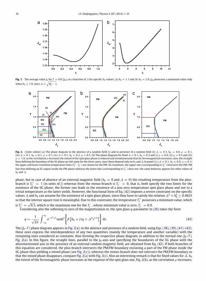
which, considered as a function of ∆, for a specific h0-value, possesses a minimum value at ∆ =

h20 − 1; this minimum is

present only for h0 ≥ 1 and its plots appear in Fig. 1. The low temperature region one has1J0

=1J00

+2T

π(1 + ∆2)2. (41)

In order to facilitate the evaluation of the phase diagram (the temperature T with respect to J0) initially we focus on theboundary between the PM (m = 0, q = 0) and SG (m = 0, q = 0) phases, which is achieved by expanding the free energy(25) in powers of q under the constraint m = 0 [14,50–52]; in this expansion the coefficient of q2-term is set equal to zeroin order to determine the respective transition temperature Tf between the aforementioned phases, yielding

Tf =

1 ±

1 − 16(∆2

+ h20)1/2

2

1/2

(42)

being J0-independent,dTfdJ0

= 0, thus representing a straight line in (J0–T )-plane. However, as it is clear from (42) thetransition temperature Tf possesses two branches, the plus-one and the minus-one; both temperatures lead to a spin glass

10 I.A. Hadjiagapiou / Physica A 397 (2014) 1–16

a b

Fig. 1. The average value J0 for T = 0 K (J00) as a function of ∆ for specific h0-values, (a) h0 = 1.1 and (b) h0 = 2.0. J00 possesses a minimum value only

when h0 ≥ 1.0, since ∆ =

h20 − 1.

a b c

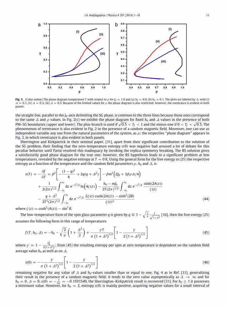
Fig. 2. (Color online) (a) The phase diagram in the absence of a random field (i) and in presence of a random field (ii) ∆ = 0.1, h0 = 0.0, ρ = 0.1,(iii) ∆ = 0.1, h0 = 0.1, ρ = 0.1, (iv) ∆ = 0.1, h0 = 0.2, ρ = 0.5. (b) The phase diagram for fixed ∆ = 0.1, h0 = 0.2 and (i) ρ = 0.0, (ii) ρ = 0.5 and (iii)ρ = 1.0; as the correlation ρ increases the extent of the spin glass phase is reduced and simultaneously that for ferromagnetism increases; also, the straightlines defining the boundary of the SG phase are the same for the three cases, since these depend only on h0 and∆. In panel (c), (∆ = 0.1, h0 = 0.0, ρ = 0.1)the upper and lower transition temperature lines (T+

f , T−

f ) are shown for the PM–SG transition; the upper one (corresponding to T+

f ) intersects the PM–FMline thus defining an SG region inside the FM-phase whereas the lower line (corresponding to T−

f ) does not; the same behavior appears for other values ofh0 and ∆.

phase, but in case of absence of an external magnetic field (h0 = 0 and ∆ = 0) the resulting temperature from the plus-branch is T+

f = 1 (in units of J) whereas from the minus-branch is T−

f = 0, that is, both specify the two limits for theexistence of the SG phase; the former one leads to the existence of a non zero temperature spin glass phase and not to atrivial temperature as the latter yields. However, the functional form of Eq. (42) imposes a severe constraint on the specificvalues ∆ and h0 can assume for the existence of a spin glass phase, since they have to satisfy the relation ∆2

+ h20 ≤ 0.0625

so that the interior square root is meaningful. Due to this constraint, the temperature T+

f possesses aminimum value, whichis T+

f =√0.5, which is the maximum one for the T−

f , whose minimum value is zero, T−

f = 0.0.Considering also the softening to zero of the magnetizationm, the spin glass q-parameter in (26) takes the form

q =1

√2π

∞

−∞

e−z2/2 tanh2

βh0 + z(q + ∆2)1/2

dz. (43)

The (J0–T ) phase diagram appears in Fig. 2(a), in the absence and presence of a random field, using Eqs. (38), (39), (41)–(43);these ones express the interdependence of any two quantities (mainly the temperature and another variable) with theremaining ones considered as constants, thus forming the respective phase diagram, in addition to the normal one (J0–T ),Fig. 2(a). In this figure, the straight lines, parallel to the J0-axis and specifying the boundaries of the SG phase with theaforementioned axis in the presence of an external random magnetic field, are obtained from Eq. (42). If both branches ofthis equation are considered, the plus-branch intersects the PM/FM boundary enclaving a part of the FM phase inside theSG phase thus yielding a mixed phase (see Fig. 2(c)), whereas the minus-branch does not intersect the PM/FM boundary sothat themixed phase disappears, compare Fig. 2(a) with Fig. 2(c). Also an interesting remark is that for fixed values for∆, h0the extent of the ferromagnetic phase increases at the expense of the spin glass one, Fig. 2(b), as the correlation ρ increases;

I.A. Hadjiagapiou / Physica A 397 (2014) 1–16 11

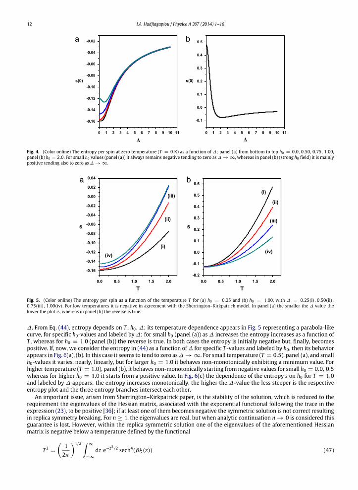
a b

Fig. 3. (Color online) The phase diagram temperature T with respect to ρ for J0 = 1.0 and (a) h0 = 0.0, (b) h0 = 0.1. The plots are labeled by ∆, with (i)∆ = 0.1, (ii) ∆ = 0.3, (iii) ∆ = 0.5. Because of the limited values for ρ the phase diagram is also restricted; however, the reentrance is evident in bothpanels.

the straight line, parallel to the J0-axis delimiting the SG phase, is common to the three lines because these ones correspondto the same ∆ and ρ values. In Fig. 2(c) we exhibit the phase diagram for fixed h0 and ∆ values in the presence of bothPM–SG boundaries (upper and lower). The plus-branch is used if

√0.5 < Tf < 1 and the minus-one if 0 < Tf <

√0.5. The

phenomenon of reentrance is also evident in Fig. 2 in the presence of a random magnetic field. Moreover, one can use asindependent variable any one from the natural parameters of the system, as ρ; the respective ‘‘phase diagram’’ appears inFig. 3, in which reentrance is also evident in both panels.

Sherrington and Kirkpatrick in their seminal paper, [31], apart from their significant contribution to the solution ofthe SG problem, their finding that the zero-temperature entropy s(0) was negative had aroused a lot of debate for thispeculiar behavior until Parisi resolved this inadequacy by invoking the replica symmetry breaking. The RS solution givesa satisfactorily good phase diagram for the true one; however, the RS hypothesis leads to a significant problem at lowtemperatures, revealed by the negative entropy at T = 0 K. Using the general form for the free energy in (25) the respectiveentropy as a function of the temperature and the random field parameters ρ, h0 and ∆, is

s(T ) = −∂ f∂T

= β2

−

(1 − q)2

4+ 2q(q + ∆2)

− βm2

2J0 + 3βρ∆/4

+

12(2π)1/2

∞

−∞

dz e−z2/2 ln4ζ (z)

−

h0 − mJ02T (2π)1/2

∞

−∞

dz e−z2/2 sinh(2A(z))ζ (z)

−q + ∆2

2T 2(2π)1/2

∞

−∞

dz e−z2/2 2ζ (z) cosh(2A(z)) − sinh2(2B)ζ (z)2

(44)

where ζ (z) = cosh2(A(z)) − sin2 B.

The low-temperature form of the spin glass parameter q is given by q ∼= 1 −

2π

T√1+∆2

[16], then the free energy (25)

assumes the following form in this range of temperatures

f (T , h0, ∆) = −h0 −

2π

1 +

∆2

2

+

γ T

π1 + ∆2

1/21 −

γ

21 + ∆2

1/2

(45)

where γ = 1 −h20

2(1+∆2); from (45) the resulting entropy per spin at zero temperature is dependent on the random field

average value h0 as well as on ∆,

s(0) = −γ

π1 + ∆2

1/21 −

γ

21 + ∆2

1/2

(46)

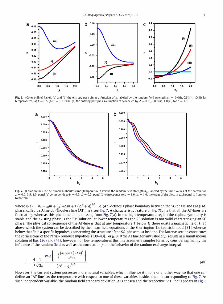
remaining negative for any value of ∆ and h0-values smaller than or equal to one, Fig. 4 as in Ref. [31], generalizingtheir result in the presence of a random magnetic field; it tends to the zero value asymptotically as ∆ → ∞ and forh0 = 0, ∆ = 0, s(0) = −

12π = −0.1591549, the Sherrington–Kirkpatrick result is recovered [31]. For h0 ≥ 1 it possesses

a minimum value. However, for h0 = 2, entropy s(0) is mainly positive, acquiring negative values for a small interval of

12 I.A. Hadjiagapiou / Physica A 397 (2014) 1–16

a b

Fig. 4. (Color online) The entropy per spin at zero temperature (T = 0 K) as a function of ∆; panel (a) from bottom to top h0 = 0.0, 0.50, 0.75, 1.00,panel (b) h0 = 2.0. For small h0 values (panel (a)) it always remains negative tending to zero as ∆ → ∞, whereas in panel (b) (strong h0 field) it is mainlypositive tending also to zero as ∆ → ∞.

a b

Fig. 5. (Color online) The entropy per spin as a function of the temperature T for (a) h0 = 0.25 and (b) h0 = 1.00, with ∆ = 0.25(i), 0.50(ii),0.75(iii), 1.00(iv). For low temperatures it is negative in agreement with the Sherrington–Kirkpatrick model. In panel (a) the smaller the ∆ value thelower the plot is, whereas in panel (b) the reverse is true.

∆. From Eq. (44), entropy depends on T , h0, ∆; its temperature dependence appears in Fig. 5 representing a parabola-likecurve, for specific h0-values and labeled by ∆; for small h0 (panel (a)) as ∆ increases the entropy increases as a function ofT , whereas for h0 = 1.0 (panel (b)) the reverse is true. In both cases the entropy is initially negative but, finally, becomespositive. If, now, we consider the entropy in (44) as a function of ∆ for specific T -values and labeled by h0, then its behaviorappears in Fig. 6(a), (b). In this case it seems to tend to zero as∆ → ∞. For small temperature (T = 0.5), panel (a), and smallh0-values it varies, nearly, linearly, but for larger h0 = 1.0 it behaves non-monotonically exhibiting a minimum value. Forhigher temperature (T = 1.0), panel (b), it behaves non-monotonically starting from negative values for small h0 = 0.0, 0.5whereas for higher h0 = 1.0 it starts from a positive value. In Fig. 6(c) the dependence of the entropy s on h0 for T = 1.0and labeled by ∆ appears; the entropy increases monotonically, the higher the ∆-value the less steeper is the respectiveentropy plot and the three entropy branches intersect each other.

An important issue, arisen from Sherrington–Kirkpatrick paper, is the stability of the solution, which is reduced to therequirement the eigenvalues of the Hessian matrix, associated with the exponential functional following the trace in theexpression (23), to be positive [36]; if at least one of them becomes negative the symmetric solution is not correct resultingin replica symmetry breaking. For n ≥ 1, the eigenvalues are real, but when analytic continuation n → 0 is considered thisguarantee is lost. However, within the replica symmetric solution one of the eigenvalues of the aforementioned Hessianmatrix is negative below a temperature defined by the functional

T 2=

12π

1/2 ∞

−∞

dz e−z2/2 sech4(βξ(z)) (47)

I.A. Hadjiagapiou / Physica A 397 (2014) 1–16 13

a b c

Fig. 6. (Color online) Panels (a) and (b) the entropy per spin as a function of ∆ labeled by the random field strength h0 = 0.0(i), 0.5(ii), 1.0(iii) fortemperatures, (a) T = 0.5, (b) T = 1.0. Panel (c) the entropy per spin as a function of h0 labeled by ∆ = 0.0(i), 0.5(ii), 1.0(iii) for T = 1.0.

a b

Fig. 7. (Color online) The de Almeida–Thouless line (temperature T versus the random field strength h0), labeled by the same values of the correlationρ = 0.0, 0.5, 1.0; panel (a) corresponds to J0 = 0.5, ∆ = 0.5; panel (b) corresponds to J0 = 1.0, ∆ = 1.0; the order of the plots in each panel is from topto bottom.

where ξ(z) = h0 + J0m +12βρ1m + z

∆2

+ q1/2. Eq. (47) defines a phase boundary between the SG phase and PM (FM)

phase, called de Almeida–Thouless line (AT line), see Fig. 7. A characteristic feature of Fig. 7(b) is that all the AT-lines arefluctuating, whereas this phenomenon is missing from Fig. 7(a). In the high temperature region the replica symmetry isstable and the existing phase is the PM solution; at lower temperatures the RS solution is not valid characterizing an SGphase. The physical consequence of the AT-line is that at any temperature T below Tf there exists a magnetic field Hc(T )above which the system can be described by the mean-field equations of the Sherrington–Kirkpatrick model [31], whereasbelow that field a specific hypothesis concerning the structure of the SG-phasemust be done. The latter assertion constitutesthe cornerstone of the Parisi–Toulouse hypothesis [39–43]. For J0 = 0 theAT line, for any value ofρ, results as a simultaneoussolution of Eqs. (26) and (47); however, for low temperatures this line assumes a simpler form, by considering mainly theinfluence of the random field as well as the correlation ρ on the behavior of the random exchange integral

T =43

1√2π

exp

−

12

h0+J0m+

12 ρ1m

2∆2+q

∆2 + q

1/2 . (48)

However, the current system possesses more natural variables, which influence it in one or another way, so that one candefine an ‘‘AT line’’ as the temperature with respect to one of these variables besides the one corresponding to Fig. 7. Assuch independent variable, the random field standard deviation ∆ is chosen and the respective ‘‘AT line’’ appears in Fig. 8

14 I.A. Hadjiagapiou / Physica A 397 (2014) 1–16

a b

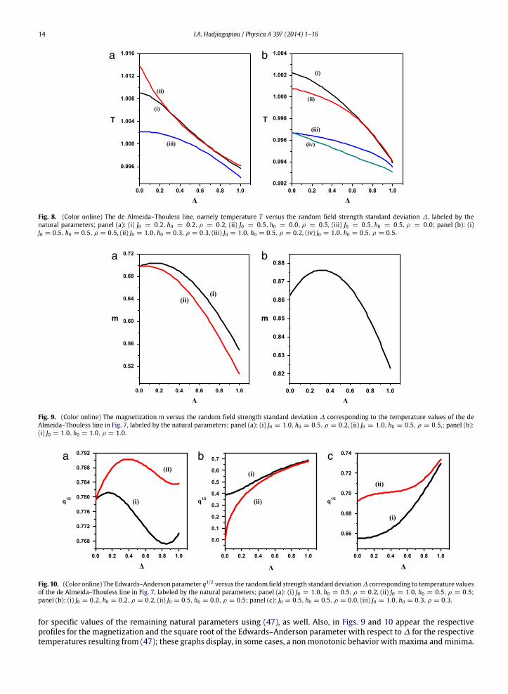
Fig. 8. (Color online) The de Almeida–Thouless line, namely temperature T versus the random field strength standard deviation ∆, labeled by thenatural parameters; panel (a): (i) J0 = 0.2, h0 = 0.2, ρ = 0.2, (ii) J0 = 0.5, h0 = 0.0, ρ = 0.5, (iii) J0 = 0.5, h0 = 0.5, ρ = 0.0; panel (b): (i)J0 = 0.5, h0 = 0.5, ρ = 0.5, (ii) J0 = 1.0, h0 = 0.3, ρ = 0.3, (iii) J0 = 1.0, h0 = 0.5, ρ = 0.2, (iv) J0 = 1.0, h0 = 0.5, ρ = 0.5.

a b

Fig. 9. (Color online) The magnetization m versus the random field strength standard deviation ∆ corresponding to the temperature values of the deAlmeida–Thouless line in Fig. 7, labeled by the natural parameters; panel (a): (i) J0 = 1.0, h0 = 0.5, ρ = 0.2, (ii) J0 = 1.0, h0 = 0.5, ρ = 0.5,; panel (b):(i) J0 = 1.0, h0 = 1.0, ρ = 1.0.

a b c

Fig. 10. (Color online) The Edwards–Anderson parameter q1/2 versus the random field strength standard deviation∆ corresponding to temperature valuesof the de Almeida–Thouless line in Fig. 7, labeled by the natural parameters; panel (a): (i) J0 = 1.0, h0 = 0.5, ρ = 0.2, (ii) J0 = 1.0, h0 = 0.5, ρ = 0.5;panel (b): (i) J0 = 0.2, h0 = 0.2, ρ = 0.2, (ii) J0 = 0.5, h0 = 0.0, ρ = 0.5; panel (c): J0 = 0.5, h0 = 0.5, ρ = 0.0, (iii) J0 = 1.0, h0 = 0.3, ρ = 0.3.

for specific values of the remaining natural parameters using (47), as well. Also, in Figs. 9 and 10 appear the respectiveprofiles for the magnetization and the square root of the Edwards–Anderson parameter with respect to ∆ for the respectivetemperatures resulting from (47); these graphs display, in some cases, a nonmonotonic behavior withmaxima andminima.

I.A. Hadjiagapiou / Physica A 397 (2014) 1–16 15

a b c

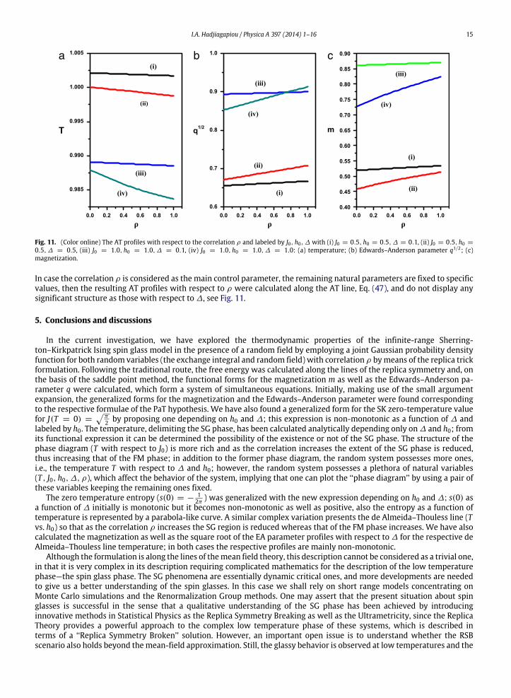
Fig. 11. (Color online) The AT profiles with respect to the correlation ρ and labeled by J0, h0, ∆ with (i) J0 = 0.5, h0 = 0.5, ∆ = 0.1, (ii) J0 = 0.5, h0 =

0.5, ∆ = 0.5, (iii) J0 = 1.0, h0 = 1.0, ∆ = 0.1, (iv) J0 = 1.0, h0 = 1.0, ∆ = 1.0: (a) temperature; (b) Edwards–Anderson parameter q1/2; (c)magnetization.

In case the correlation ρ is considered as the main control parameter, the remaining natural parameters are fixed to specificvalues, then the resulting AT profiles with respect to ρ were calculated along the AT line, Eq. (47), and do not display anysignificant structure as those with respect to ∆, see Fig. 11.

5. Conclusions and discussions

In the current investigation, we have explored the thermodynamic properties of the infinite-range Sherring-ton–Kirkpatrick Ising spin glass model in the presence of a random field by employing a joint Gaussian probability densityfunction for both random variables (the exchange integral and random field) with correlation ρ bymeans of the replica trickformulation. Following the traditional route, the free energy was calculated along the lines of the replica symmetry and, onthe basis of the saddle point method, the functional forms for the magnetization m as well as the Edwards–Anderson pa-rameter q were calculated, which form a system of simultaneous equations. Initially, making use of the small argumentexpansion, the generalized forms for the magnetization and the Edwards–Anderson parameter were found correspondingto the respective formulae of the PaT hypothesis. We have also found a generalized form for the SK zero-temperature valuefor J(T = 0) =

π2 by proposing one depending on h0 and ∆; this expression is non-monotonic as a function of ∆ and

labeled by h0. The temperature, delimiting the SG phase, has been calculated analytically depending only on ∆ and h0; fromits functional expression it can be determined the possibility of the existence or not of the SG phase. The structure of thephase diagram (T with respect to J0) is more rich and as the correlation increases the extent of the SG phase is reduced,thus increasing that of the FM phase; in addition to the former phase diagram, the random system possesses more ones,i.e., the temperature T with respect to ∆ and h0; however, the random system possesses a plethora of natural variables(T , J0, h0, ∆, ρ), which affect the behavior of the system, implying that one can plot the ‘‘phase diagram’’ by using a pair ofthese variables keeping the remaining ones fixed.

The zero temperature entropy (s(0) = −12π ) was generalized with the new expression depending on h0 and ∆; s(0) as

a function of ∆ initially is monotonic but it becomes non-monotonic as well as positive, also the entropy as a function oftemperature is represented by a parabola-like curve. A similar complex variation presents the de Almeida–Thouless line (Tvs. h0) so that as the correlation ρ increases the SG region is reduced whereas that of the FM phase increases. We have alsocalculated the magnetization as well as the square root of the EA parameter profiles with respect to ∆ for the respective deAlmeida–Thouless line temperature; in both cases the respective profiles are mainly non-monotonic.

Although the formulation is along the lines of themean field theory, this description cannot be considered as a trivial one,in that it is very complex in its description requiring complicated mathematics for the description of the low temperaturephase—the spin glass phase. The SG phenomena are essentially dynamic critical ones, and more developments are neededto give us a better understanding of the spin glasses. In this case we shall rely on short range models concentrating onMonte Carlo simulations and the Renormalization Group methods. One may assert that the present situation about spinglasses is successful in the sense that a qualitative understanding of the SG phase has been achieved by introducinginnovative methods in Statistical Physics as the Replica Symmetry Breaking as well as the Ultrametricity, since the ReplicaTheory provides a powerful approach to the complex low temperature phase of these systems, which is described interms of a ‘‘Replica Symmetry Broken’’ solution. However, an important open issue is to understand whether the RSBscenario also holds beyond themean-field approximation. Still, the glassy behavior is observed at low temperatures and the

16 I.A. Hadjiagapiou / Physica A 397 (2014) 1–16

phenomenology much resembles the one of some mean-field spin glass models. For this reason, concepts and techniquesfrom spin glasses have been widely applied to investigate glassy behavior in these systems.

The current investigation shall be extended towards the Replica Symmetry Breaking formulation.

Acknowledgment

This research was supported by the Special Account for Research Grants of the University of Athens (EΛKE) under GrantNo. 70/4/4096.

References

[1] R.B. Stinchcombe, in: C. Domb, J.L. Lebowitz (Eds.), Phase Transitions and Critical Phenomena, Vol. 7, Academic Press, London, 1983.[2] Vik.S. Dotsenko, Vl.S. Dotsenko, Adv. Phys. 32 (1983) 129.[3] Y. Imry, M. Wortis, Phys. Rev. B 19 (1979) 3580.[4] I.A. Hadjiagapiou, A. Malakis, S.S. Martinos, Physica A 387 (2008) 2256.[5] I.A. Hadjiagapiou, Physica A 390 (2011) 1279.[6] I.A. Hadjiagapiou, Physica A 389 (2010) 3945. 392 (2013) 1063.[7] N.G. Fytas, V. Martín-Mayor, Phys. Rev. Lett. 110 (2013) 227201.[8] N.G. Fytas, P.E. Theodorakis, I. Georgiou, Eur. Phys. J. B 85 (2012) 349.[9] K. Bannora, G. Ismail, W. Hassan, Chin. Phys. B 20 (2011) 067501.

[10] D.S. Fisher, G.M. Grinstein, A. Khurana, Phys. Today 41 (12) (1988) 56.[11] Y. Imry, S.-K. Ma, Phys. Rev. Lett. 35 (1975) 1399.[12] A. Aharony, Phys. Rev. B 18 (1978) 3318.[13] H. Nishimori, G. Ortiz, Elements of Phase Transitions and Critical Phenomena, Oxford University Press, Oxford, 2011.[14] K. Binder, A.P. Young, Rev. Modern Phys. 58 (1986) 801.[15] K. Binder, Festkörperprobleme XVII (1977) 55.[16] H. Nishimori, Statistical Physics of Spin Glasses and Information Processing, Oxford University Press, Oxford, 2001.[17] M. Mezard, G. Parisi, M.A. Virasoro, Spin Glasse Theory and Beyond, World Scientific, Singapore, 1987.[18] K.H. Fischer, J.A. Hertz, Spin Glasses, Cambridge University Press, London, 1991.[19] I.Ya. Korenblit, E.F. Shender, Sov. Phys. Usp. 32 (1989) 139.[20] S. Fishman, A. Aharony, J. Phys. C 12 (1979) L729.[21] J.Z. Imbrie, Phys. Rev. Lett. 53 (1984) 1747.[22] S. Galam, Phys. Rev. B 31 (1985) 7274.[23] M. Gofman, J. Adler, A. Aharony, A.B. Harris, M. Schwartz, Phys. Rev. Lett. 71 (1993) 2841; Phys. Rev. B 53 (1996) 6362.[24] A. Houghton, A. Khurana, F.J. Seco, Phys. Rev. B 34 (1986) 1700.[25] J. Machta, M.E.J. Newman, L.B. Chayes, Phys. Rev. E 62 (2000) 8782.[26] A.A. Middleton, D.S. Fisher, Phys. Rev. B 65 (2002) 134411.[27] A. Malakis, N.G. Fytas, Phys. Rev. E 73 (2006) 016109; Eur. Phys. J. B 50 (2006) 39.[28] H. Nishimori, Progr. Theoret. Phys. 66 (1981) 1169; J. Phys. Soc. Japan 80 (2011) 023002.[29] T. Kaneyoshi, J. Phys. C 9 (1976) L289.[30] S.F. Edwards, P.W. Anderson, J. Phys. F: Met. Phys. 5 (1975) 965.[31] D. Sherrington, S. Kirkpatrick, Phys. Rev. Lett. 35 (1975) 1792; Phys. Rev. B 17 (1978) 4384.[32] J.L. van Hemmen, R.G. Palmer, J. Phys. A 12 (1979) 563.[33] K. Wada, H. Takayama, Progr. Theoret. Phys. 64 (1980) 327.[34] G. Parisi, Phys. Rev. Lett. 43 (1979) 1754; J. Phys. A 13 (1980) 1101, 1887.[35] D.J. Thouless, P.W. Anderson, R.G. Palmer, Phil. Mag. 35 (1977) 593.[36] J.R.L. de Almeida, D.J. Thouless, J. Phys. A 11 (1978) 983.[37] F.L. Toninelli, Europhys. Lett. 60 (2002) 764.[38] H. Kato, M. Okada, S. Miyoshi, J. Phys. Soc. Japan 82 (2013) 074802.[39] G. Parisi, G. Toulouse, J. Physique Lett. 41 (1980) L-361.[40] J. Vannimenus, G. Toulouse, G. Parisi, J. Physique 42 (1981) 565.[41] P. Monod, H. Bouchiat, J. Physique Lett. 43 (1982) L-45.[42] K.H. Fischer, Phys. Status Solidi B 116 (1983) 357.[43] S.-K. Ma, M. Payne, Phys. Rev. B 24 (1981) 3984.[44] R.F. Soares, F.D. Nobre, J.R.L. de Almeida, Phys. Rev. B 50 (1994) 6151;

E. Nogueira Jr., F.D. Nobre, F.A. da Costa, S. Coutinho, Phys. Rev. E 57 (1998) 5079;J.M. de Araújo, F.D. Nobre, F.A. da Costa, Phys. Rev. E 61 (2000) 2232.

[45] R. Pirc, B. Tadic, R. Blinc, Phys. Rev. B 36 (1987) 8607; Physica A 185 (1992) 322.[46] D.-H. Kim, J.-J. Kim, Ferroelectrics 268 (2002) 263; Phys. Rev. B 66 (2002) 054432.[47] A.P. Young (Ed.), Spin Glasses, World Scientific, Singapore, 1997.[48] F. Lefloch, J. Hammann, M. Ocio, E. Vincent, Physica B 203 (1994) 63.[49] J.O. Piatek, B. Dalla Piazza, N. Nikseresht, T. Tsyrulin, I. Zivković, K.W. Krämer, M. Laver, K. Prokes, S. Matas, N.B. Christensen, H.M. Rønnow, Phys. Rev.

B 88 (2013) 014408.[50] M. Suzuki, Progr. Theoret. Phys. 58 (1977) 1151.[51] S. Nabu, S. Naya, Progr. Theoret. Phys. 63 (1980) 1098.[52] S. Nabu, Progr. Theoret. Phys. 63 (1980) 1474.