the seventeen provers of the worldfreek/comparison/comparison.pdf · the seventeen provers of the...
TRANSCRIPT

The Seventeen Provers of the World
Compiled by Freek Wiedijk(and with a Foreword by Dana Scott)
Radboud University Nijmegen
Abstract. We compare the styles of several proof assistants for math-ematics. We present Pythagoras’ proof of the irrationality of
√2 both
informal and formalized in (1) HOL, (2) Mizar, (3) PVS, (4) Coq, (5) Ot-ter/Ivy, (6) Isabelle/Isar, (7) Alfa/Agda, (8) ACL2, (9) PhoX, (10) IMPS,(11) Metamath, (12) Theorema, (13) Lego, (14) Nuprl, (15) Ωmega, (16)B method, (17) Minlog.
proof assistant author of proof page
informal Henk Barendregt 171 HOL John Harrison, Konrad Slind, Rob Arthan 182 Mizar Andrzej Trybulec 273 PVS Bart Jacobs, John Rushby 314 Coq Laurent Thery, Pierre Letouzey, Georges Gonthier 355 Otter/Ivy Michael Beeson, William McCune 446 Isabelle/Isar Markus Wenzel, Larry Paulson 497 Alfa/Agda Thierry Coquand 588 ACL2 Ruben Gamboa 639 PhoX Christophe Raffalli, Paul Roziere 76
10 IMPS William Farmer 8211 Metamath Norman Megill 9812 Theorema Wolfgang Windsteiger, Bruno Buchberger, Markus
Rozenkranz 10613 Lego Conor McBride 11814 Nuprl Paul Jackson 12715 Ωmega Christoph Benzmuller, Armin Fiedler, Andreas
Meier, Martin Pollet, Jorg Siekmann 13916 B method Dominique Cansell 15417 Minlog Helmut Schwichtenberg 163
Foreword
by Dana S. Scott <[email protected]>University Professor EmeritusCarnegie Mellon UniversityPittsburgh, Pennsylvania, USA
Our compiler, Freek Wiedijk, whom everyone interested in machine-aided de-duction will thank for this thought-provoking collection, set his correspondentsthe problem of proving the irrationality of the square root of 2. That is a nice,straight-forward question. Let’s think about it geometrically – and intuitively.
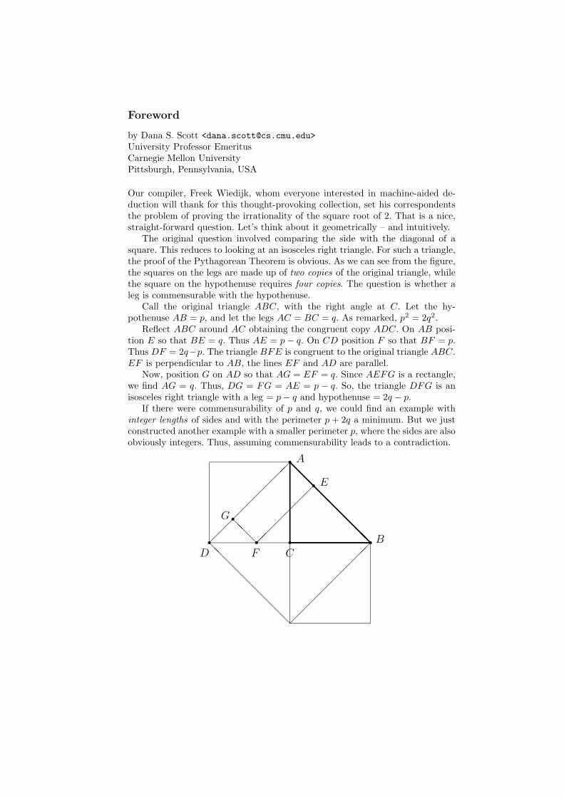
The original question involved comparing the side with the diagonal of asquare. This reduces to looking at an isosceles right triangle. For such a triangle,the proof of the Pythagorean Theorem is obvious. As we can see from the figure,the squares on the legs are made up of two copies of the original triangle, whilethe square on the hypothenuse requires four copies. The question is whether aleg is commensurable with the hypothenuse.
Call the original triangle ABC, with the right angle at C. Let the hy-pothenuse AB = p, and let the legs AC = BC = q. As remarked, p2 = 2q2.
Reflect ABC around AC obtaining the congruent copy ADC. On AB posi-tion E so that BE = q. Thus AE = p − q. On CD position F so that BF = p.Thus DF = 2q−p. The triangle BFE is congruent to the original triangle ABC.EF is perpendicular to AB, the lines EF and AD are parallel.
Now, position G on AD so that AG = EF = q. Since AEFG is a rectangle,we find AG = q. Thus, DG = FG = AE = p − q. So, the triangle DFG is anisosceles right triangle with a leg = p − q and hypothenuse = 2q − p.
If there were commensurability of p and q, we could find an example withinteger lengths of sides and with the perimeter p + 2q a minimum. But we justconstructed another example with a smaller perimeter p, where the sides are alsoobviously integers. Thus, assuming commensurability leads to a contradiction.
r A
r Br
C
r
D
r E
r
F
rG
¡¡¡¡¡¡¡¡¡
@@
@@
@@
@@@¡¡¡¡¡¡¡¡¡
¡¡
¡¡
¡¡¡@
@@
@@
@@
@@
@@@
@@
@@
@@
@@@
Foreword 3
As one of the contributors remarks, this reduction of (p, q) to (p − q, 2q − p)is very, very easy to accomplish with algebra – and the observation avoids thelemmas about even and odd numbers in finishing the required proof. But, whatdoes this really mean? As I have often told students, “Algebra is smarter thanyou are!” By which I mean that the laws of algebra allow us to make many stepswhich combine information and hide tracks after simplifications, especially bycancellation. Results can be surprising, as we know from, say, the technique ofgenerating functions.
In the case of the isosceles right triangle (from the diagonal of the square),an illumination about meaning can be obtained best from thinking about theEuclidean Algorithm. For a pair of commensurable magnitudes (a, b), the find-ing of “the greatest common measure” can be accomplished by setting up asequence of pairs, starting with (a, b), and where the next pair is obtained fromthe preceding one by subtracting the smaller magnitude from the larger – and byreplacing the larger by this difference. When, finally, equal pairs are found, thisis the desired greatest common measure. (And, yes, I know this can be speededup by use of the Division Algorithm.)
In our case we would have: (p, q), (p−q, q), (p−q, 2q−p), . . . . If we do somecalculation with ratios (as the ancient Greeks knew how to do), we remark thatthe Pythagorean Theorem gives us first p/q = 2q/p. (Look at the triangles tosee this: all isosceles right triangles are similar!) From this follows (p − q)/q =(2q − p)/p. Now switch extremes to conclude that p/q = (2q − p)/(p − q). Thisshows that the third term of our run of the Euclidean Algorithm gives a pairwith the same ratio (when the larger is compared with the smaller) as for theinitial pair. In any run of the Euclidean Algorithm, if a ratio ever repeats, thenthe algorithm never finishes. Why? Because the pattern of larger and smallerquantities is going to repeat and, thus, no equals will be found. Hence, themagnitudes of the original pair are incommensurable. Indeed, Exodus knew thata/b = c/d could be defined by saying that the two runs of the algorithm startingwith (a, b)and(c, d), respectively, have the same patterns of larger and smaller.
In later centuries it was recognized that the Euclidean Algorithm is directlyconnected with the (simple) continued fraction expansion. Moreover, as Lagrangeshowed, the infinite, eventually periodic, simple continued fractions give exactlythe positive irrational roots of quadratic equations (with integer coefficients).Perhaps, then, it might have been a more interesting challenge to prove theLagrange Theorem itself, but probably fewer groups would have responded.
Alas, I have never spent any extended time with the provers/checkers repre-sented in this collection. I did invest many profitable hours in using the equa-tional theorem prover, Waldmeister: it is small, yet very effective on manyproblems involving equational deductions. Unfortunately, some theorem proversbased on first-order logic do not really incorporate all the techniques of equa-tional provers, so with certain problems time and/or space may run out beforefinding a proof. It is imperative that implementers of these systems now takeadvantage of specialized algorithms if ever mathematicians are going to becomeinterested in using a machine-based method.
4 Dana Scott
We can also see clearly from the examples in this collection that the notationsfor input and output have to be made more human readable. Several systems dogenerate LaTeX output for the discovered proofs, but perhaps additional thoughtabout formatting output might be valuable. The Theorema Project (system 12in the present list) made readablity of proofs a prime requirement, and theirreport shows their success. However, the objective Prof. Bruno Buchberger setoriginally for the project was to produce a tool for pedagogic use, not research.Thus, the power of their system does not yet reach what, say, the HOL-basedsystems surveyed in this report have. Also, the question of the discovery of aproof is different from checking a proffered proof. Hence, any features that makea system interactive – and many in this collection have such – do help in findingproofs through experimentation.
Over about a decade I developed undergraduate courses using Mathemat-ica. One effort was directed at Discrete Mathematics, and my colleague, KlausSutner, at Carnegie Mellon has expanded that effort several fold with excellentsuccess. Most of my own thought went into a course on Projective Geometry,basically an introduction to plane algebraic curves over the complex field. WhatI found via the use of computer algebra was that theorems can be proved byasking for simplifications and interaction between equations. Technically, I usednot just commutative algebra but also an implementation of the algebra of par-tial differential operators acting on multivariate polynomials. The details are notimportant, as the point was that the user of Mathematica had to enter the rightquestions and control the choices of appropriate cases (say, after a factoriza-tion of a polynomial) in order to reach the desired conclusions. In other words,though there was automatic verification and generation of algebraic facts, thereis not a deductive facility built into Mathematica. And I wish there were! Somevery good progress has been made in the system, however, in simplifications oflogical formulae involving the equations and inequalities over the real field. Butwelcome as this is, it is not general-purpose logical deduction.
Computer algebra systems have become very powerful and are used bothfor applications (say, in computer-aided design of complicated surfaces) and inresearch (say, in group theory, for example). But we have to note that thougheffective, proofs are not generated. The user of the system has to believe that thesystem is doing the simplifications correctly. Usually we are able to accept resultson faith, and we are happy to see what is discovered, but, strictly speaking, aproof is lacking. For a wide-ranging discussion of such issues, the reader mayconsult “A Skeptic’s Approach to Combining HOL and Maple” by John Harrisonand Laurent Thery, which appeared in Journal of Automated Reasoning, vol. 21(1998), pp. 279–294. (This is also to be found on John Harrison’s WWW page.)
So we have here is a dilemma to be faced by implementors of proof systems.On the one hand, interaction and experimentation can be considerably speededup by using automatic simplification of logical and algebraic expressions – andone can hope even by rules that the user specifies himself. Alternately, newmethods for large-scale Boolean satisfaction algorithms might be employed. Onthe other hand, for verification (either by humans or by another part of the
Foreword 5
system), checkable proofs have to be generated and archived. Computers are sofast now that hundreds of pages of steps of simplifications can be recorded evenfor simple problems. Hence, we are faced with the questions, “What really is aproof?” and “How much detail is needed?” Several different answers are offeredby the systems surveyed here. But, is there a canonical answer that will satisfythe test of time – and be relevant as new systems are put forward in the future?And don’t forget that probabilistic proof procedures (say, for checking whethera large number is prime) also involve the question of what constitutes a proof.
Large searches present another vexing block for understanding what a systemhas accomplished. The original attack by computer on the Four Color Conjec-ture is a case in point. As discussed in the introduction by Wiedijk, objectionshave now been eliminated by showing that the method for generating the nec-essary cases is correct, even though the total run of the program is not humanlysurveyable. On the other hand, as noted, work by Hales to eliminate criticismsof his solution to Kepler’s Conjecture, though making progress, still continues.Of course, there will always be people who will say such computer calculation,no matter how well designed – and with verified design principles – do not re-ally give us proofs. They may even say, “How do you know that there was notsome quantum-mechanical glitch that threw the computer off?” Running theprogram again with the same results will not be convincing either. But, what Ithink will silence the nay-sayers is the development of whole suites of general-purpose programs for solving new problems. Not to criticize the work on FourColor Conjecture or on Kepler’s Conjecture, but it often seems that a big ef-fort is put into solving one single problem, and that’s it. When proof assistantsconstitute a research tool that (suitably minded) mathematicians use daily forwork, then there will be recognition and acceptance. This has already happenedfor computer-algebra systems and for chip-design verification systems. I remainoptimistic that we will sooner and not later see real progress with solid mathe-matics proof systems.
But human imagination can always outstrip the capabilities of machines.To bring this point home in a very clear way, I think that the two delightfulbooks by Roger B. Nelson, Proofs Without Words: Exercises in Visual Thinking(1993) and Proofs Without Words II: More Exercises in Visual Thinking (2000),published by The Mathematical Association of America, can give a deep fund ofexamples and questions about how proofs can be formalized. In the books thereare, of course, many of the proofs of the Pythagorean Theorem, probably themost proved theorem in mathematics. Two I especially like involve facts aboutsimilar triangles: see proof VI on p. 8 of the first volume, and XI on p. 7 of thesecond. Proofs like these involve augmenting the original figure by what are oftencalled “auxiliary lines”. I particularly hated this method of proof in geometrywhen I first saw it in school. The teacher would introduce these constructions ina way like a magician pulling a rabbit out of a hat. It did not seem fair to makea hard problem easy, because there was little made obvious about where thesehelpers came from. After a while, I learned to do this stuff myself, and then Iliked it. But training machines to do this is another question.
6 Dana Scott
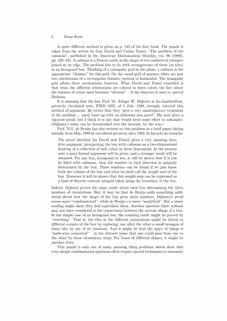
A quite different method is given on p. 142 of the first book. The puzzle istaken from the article by Guy David and Carlos Tomei, “The problem of thecalissons”, published in the American Mathematical Monthly, vol. 96 (1989),pp. 429–431. A calisson is a French candy in the shape of two equilateral trianglesjoined at an edge. The problem has to do with arrangements of these (as tiles)in an hexagonal box. Thinking of a triangular grid in the plane, a calisson is theappropriate “domino” for this grid. On the usual grid of squares, there are justtwo orientations of a rectangular domino: vertical or horizontal. The triangulargrid allows three orientations, however. What David and Tomei remarked isthat when the different orientations are colored in three colors, the fact aboutthe balance of colors used becomes “obvious” – if the observer is used to opticalillusions.
It is amusing that the late Prof. Dr. Edsger W. Dijkstra in his handwritten,privately circulated note, EWD 1055, of 5 July, 1989, strongly rejected thismethod of argument. He writes that they “give a very unsatisfactory treatmentof the problem ... [and] come up with an elaborate non proof.” His note gives arigorous proof, but I think it is one that would need some effort to automate.(Dijkstra’s notes can be downloaded over the internet, by the way.)
Prof. N.G. de Bruijn has also written on this problem in a brief paper datinginitially from May, 1989 he circulated privately after 1994. In his note he remarks:
The proof sketched [by David and Tomei] gives a very amusing intu-itive argument, interpreting the box with calissons as a two-dimensionaldrawing of a collection of unit cubes in three dimensions. In the presentnote a more formal argument will be given, and a stronger result will beobtained. For any box, hexagonal or not, it will be shown that if it canbe filled with calissons, then the number in each direction is uniquelydetermined by the box. These numbers can be found if we just knowboth the volume of the box and what we shall call the weight sum of thebox. Moreover it will be shown that this weight sum can be expressed asa kind of discrete contour integral taken along the boundary of the box.
Indeed, Dijkstra proves the same result about each box determining the threenumbers of orientations. But, it may be that de Bruijn adds something addi-tional about how the shape of the box gives these numbers. Dijkstra’s proofseems more “combinatorial”, while de Bruijn’s is more “analytical”. But a closerreading might show they had equivalent ideas. Another question these authorsmay not have considered is the connections between the various tilings of a box.In the simple case of an hexagonal box, the counting result might be proved by“rewriting”. That is, the tiles in the different orientations might be driven todifferent corners of the box by replacing, one after the other a small hexagon ofthree tiles by one of its rotations. And it might be that the space of tilings is“path-wise connected” – in the discrete sense that one could pass from one tothe other by these elementary steps. For boxes of different shapes, it might beanother story.
This puzzle is only one of many amusing tiling problems which show thateven simple combinatorial questions often require special techniques to automate
Foreword 7
owing to the large number of possible configurations to be considered, as manyauthors have remarked. In many cases, the solutions do not depend on generaltheorems but require searches crafted solely for the particular problem. Theproblem of the calissons may be an example in between; if so, it might be moreinteresting to study than those requiring “brute force”. And all such examplesmake us again ask: “What is a (good) proof?”
Note added 22 May 2005.
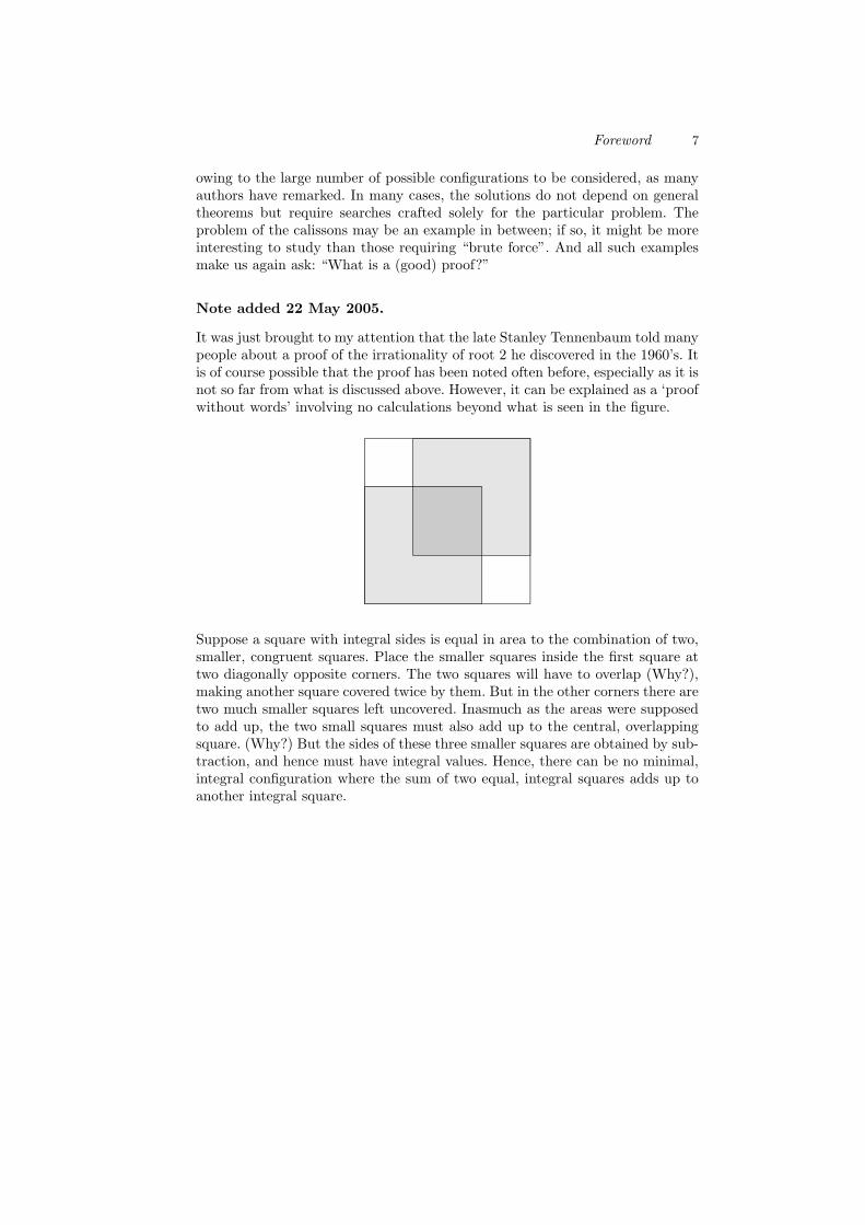
It was just brought to my attention that the late Stanley Tennenbaum told manypeople about a proof of the irrationality of root 2 he discovered in the 1960’s. Itis of course possible that the proof has been noted often before, especially as it isnot so far from what is discussed above. However, it can be explained as a ‘proofwithout words’ involving no calculations beyond what is seen in the figure.
Suppose a square with integral sides is equal in area to the combination of two,smaller, congruent squares. Place the smaller squares inside the first square attwo diagonally opposite corners. The two squares will have to overlap (Why?),making another square covered twice by them. But in the other corners there aretwo much smaller squares left uncovered. Inasmuch as the areas were supposedto add up, the two small squares must also add up to the central, overlappingsquare. (Why?) But the sides of these three smaller squares are obtained by sub-traction, and hence must have integral values. Hence, there can be no minimal,integral configuration where the sum of two equal, integral squares adds up toanother integral square.
I want HOL Light to be both a cute little toy
and a macho heavyweight industrial prover.
— JOHN HARRISON
Introduction
by Freek Wiedijk <[email protected]>
Some years ago during lunch, Henk Barendregt told me about a book (Algorith-mics by David Harel) that compared programming languages by showing thesame little program in each language that was treated. Then I thought: I coulddo that for proof assistants! And so I mailed various people in the proof assistantcommunity and started the collection that is now in front of you.
In the QED manifesto a future is sketched in which all mathematics is rou-tinely developed and checked using proof assistants. In the comparison that youare now reading all systems have been included that one should look at whenone is serious about trying to bring this QED utopia closer. That means thatthose systems are included that satisfy two criteria:
– They are designed for the formalization of mathematics, or, if not designedspecifically for that, have been seriously used for this purpose in the past.
– They are special at something. These are the systems that in at least onedimension are better than all the other systems in the collection. They arethe leaders in the field.
I called those systems the provers of the world.Some of the people that I asked for a formalization replied to my mail by
saying something like, ‘Why should we do all this work for you? If you want aformalization, you go make it yourself!’ But then I guessed that if the trivialproof that I was asking them for is not quite trivial in their system, then theirsystem is not really suited for mathematics in the first place, so it then fails myfirst criterion, and it should not be included.
The formalizations are included in this collection in the order that I receivedthem. In particular, I got the HOL and Mizar formalizations back on the sameday that I sent my request (‘Nice idea! Here it is!’) However, I did not sendall requests immediately: originally I only had nine systems. But then peoplepointed out systems that I had overlooked, and I thought of a few more myselftoo. So the collection grew.
I did not want to write any of the formalizations myself, as I wanted theformalizations to be ‘native’ to the system. I am a Coq/Mizar user, so my for-malizations would have been too ‘Coq-like’ or ‘Mizar-like’ to do justice to theother systems (and even a Coq formalization by me would probably be too‘Mizar-like’, while a Mizar formalization would be too ‘Coq-like’.)
Introduction 9
I had to select what proof to take for this comparison of formalizations. Thereare two canonical proofs that are always used to show non-mathematicians whatmathematical proof is:
– The proof that there are infinitely many prime numbers.– The proof of the irrationality of the square root of two.
From those two I selected the second, because it involves the real numbers. It isa lot of work to formalize the real numbers, so it is interesting which systemshave done that work, and how it has turned out. In fact, not all systems in thiscollection have the real numbers available. In those systems the statement thatwas formalized was not so much the irrationality of the square root of two:
√2 6∈ Q
as well just the key lemma that if a square is twice another square, then bothare zero:
m2 = 2n2 ⇐⇒ m = n = 0
I did not ask for a formalization of any specific proof. That might have givenan unjustified bias to some of the systems. Instead, I just wrote about ‘thestandard proof by Euclid’.1 With this I did not mean to refer to any actualhistorical proof of the theorem, I just used these words to refer to the theorem.I really intended everyone to take the proof that they thought to be the mostappropriate. However, I did ask for a proof that was ‘typical’ for the system,that would show off how the system was meant to be used.
At first I just created a LATEX document out of all the files that I got, butthen I decided that it would be nice to have a small description of the systems togo with the formalizations. For this reason I compiled a ‘questionnaire’, a list ofquestions about the systems. I then did not try to write answers myself, but gotthem from the same people who gave me the formalizations. This means thatthe answers vary in style. Hopefully they still provide useful information aboutthe systems.
The comparison is very much document-centric. It does not primarily focuson the interface of the systems, but instead focuses on what the result of proofformalization looks like. Also, it does not focus on what the result can be madeto look like, but instead on what the proof looks like when the user of the systeminteracts with it while creating it. It tries to show ‘the real stuff’ and not onlythe nice presentations that some systems can make out of it.
Most formalizations needed a few lemmas that ‘really should have been inthe standard library of the system’. We show these lemmas together with theformalized proof: we really try to show everything that is needed to check theformalization on top of the standard library of the system.
1 In fact the theorem does not originate with Euclid but stems from the Pythagoreantradition. Euclid did not even put it explicitly in his Elements (he probably wouldhave viewed it as a trivial consequence of his X.9), although it was later added to itby others.
10 Freek Wiedijk
One of the main aims of this comparison is comparing the appearance ofproofs in the various systems. In particular, it is interesting how close that man-ages to get to non-formalized mathematics. For this reason there is also an‘informal’ presentation of the proof included, as Section 0. On pp. 39–40 of the4th edition of Hardy and Wright’s An Introduction to the Theory of Numbers,one finds a proof of the irrationality of
√2 (presented for humans instead of for
computers):
Theorem 43 (Pythagoras’ theorem).√
2 is irrational.The traditional proof ascribed to Pythagoras runs as follows. If
√2 is
rational, then the equationa2 = 2b2 (4.3.1)
is soluble in integers a, b with (a, b) = 1. Hence a2 is even, and thereforea is even. If a = 2c, then 4c2 = 2b2, 2c2 = b2, and b is also even, contraryto the hypothesis that (a, b) = 1. 2
Ideally, a computer should be able to take this text as input and check it for itscorrectness. We clearly are not yet there. One of the reasons for this is that thisversion of the proof does not have enough detail. Therefore, Henk Barendregtwrote a very detailed informal version of the proof as Section 0. Again, ideallya proof assistant should be able to just check Henk’s text, instead of the more‘computer programming language’ like scripts that one needs for the currentproof assistants.
There are various proofs of the irrationality of√
2. The simplest proof reasonsabout numbers being even and odd.2 However, some people did not just formalizethe irrationality of
√2, but generalized it to the irrationality of
√p for arbitrary
prime numbers p. (Sometimes I even had to press them to specialize this to theirrationality of
√2 at the end of their formalization.)
Conor McBride pointed out to me that if one proves the irrationality of√
pthen there are two different properties of p that one can take as a assumptionabout p. The p can be assumed to be irreducible (p has just divisors 1 anditself), or it can be assumed to be prime (if p divides a product, it alwaysdivides one of its factors).3 Conor observed that proving the irrationality of
√p
where the assumption about p is that it is prime, is actually easier than provingthe irrationality of
√2, as the hard part will then be to prove that 2 is prime.
Rob Arthan told me that a nicer generalization than showing the irrationalityof
√p for prime p, is to show that if n is an integer and
√n is not, then this√
n is in fact irrational. According to him at a very detailed level this is evenslightly easier to prove than the irrationality of prime numbers.
I had some discussion with Michael Beeson about whether the proof of theirrationality of
√2 necessarily involves an inductive argument. Michael convinced
2 This becomes especially easy when a binary representation for the integers is used.3 In ring theory one talks about ‘irreducible elements’ and ‘prime ideals’, and this is
the terminology that we follow here. In number theory a ‘prime number’ is gener-ally defined with the property of being ‘an irreducible element’, but of course bothproperties characterize prime numbers there.
Introduction 11
me in the end that it is reasonable to take the lemma that every fraction canbe put in lowest terms (which itself generally also is proved with induction) asbackground knowledge, and that therefore the irrationality proof can be givenwithout an inductive argument. The Hardy & Wright proof seems to show thatthis also is how mathematicians think about it.
Each section in this document follows the same structure. They are all di-vided into four subsections. The third subsection is the main thing: it is theformalization, typeset as closely as possible as it appears in the files that peoplesent me. However, that subsection sometimes is quite long and incomprehensi-ble. For clarity I wanted to highlight the syntax of statements, and the syntaxof definitions. For this reason, I took the final statement that was proved, andsome sample definitions from the formalization or system library, and put themin the first and second subsections. Therefore, those first two subsections arenot part of the formalization, but excerpts from the third subsection. The fourthsubsection, finally, is the description of the system in the form of answers to thequestionnaire.
One of the main reasons for doing the comparison between provers is that Ifind it striking how different they can be. Seeing HOL, Mizar, Otter, ACL2 andMetamath next to each other, I feel that they hardly seem to have something incommon. When one only knows a few systems, it is tempting to think that allproof assistants necessarily have to be like that. The point of this comparison isthat this turns out not to be the case.
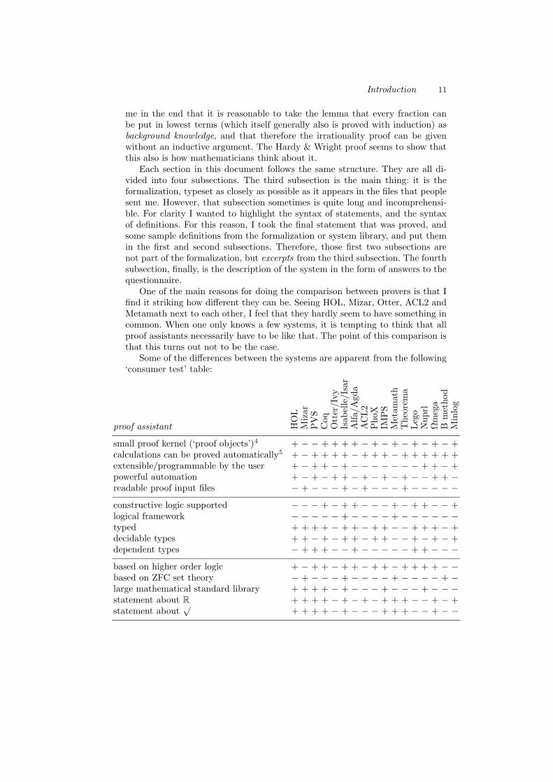
Some of the differences between the systems are apparent from the following‘consumer test’ table:
proof assistant HO
LM
izar
PV
SC
oq
Ott
er/I
vy
Isab
elle
/Isa
rA
lfa/
Agd
aA
CL2
PhoX
IMP
SM
etam
ath
Theo
rem
aLeg
oN
uprl
Ωm
ega
Bm
ethod
Min
log
small proof kernel (‘proof objects’)4 + − − + + + + − + − + − + − + − +calculations can be proved automatically5 + − + + + + − + + + − + + + + + +extensible/programmable by the user + − + + − + − − − − − − − + + − +powerful automation + − + − + + − + − + − + − − + + −readable proof input files − + − − − + − + − − − + − − − − −constructive logic supported − − − + − + + − − − + − + + − − +logical framework − − − − − + − − − − + − − − − − −typed + + + + − + + − + + − − + + + − +decidable types + + − + − + + − + + − − + − + − +dependent types − + + + − − + − − − − − + + − − −based on higher order logic + − + + − + + − + + − + + + + − −based on ZFC set theory − + − − − + − − − − + − − − − + −large mathematical standard library + + + + − + − − − + − − − + − − −statement about R + + + + − + − + − + + + − − + − +statement about
√+ + + + − + − − − + + + − − + − −
12 Freek Wiedijk
Some of the properties shown in this table (like ‘powerful automation’ and ‘largelibrary’) are rather subjective, but we still hope that the table gives some indica-tion about the variation between the systems. For instance, some people believethat ‘ZF style’ set theory is only a theoretical vehicle, and cannot be used to dorealistic proofs. But this table shows that four of the systems are in fact able toformalize a lot of real mathematics on such a set theoretical foundation!
The systems in this comparison are all potential candidates for realization of aQED manifesto-like future. However, in this comparison only very small proofs inthese systems are shown. Recently some very large proofs have been formalized,and in this introduction we would like to show a little bit of that as well. Theseformalizations were all finished at the end of 2004 and the beginning of 2005.
Prime Number Theorem. This formalization was written by Jeremy Avigadof Carnegie Mellon University, with the help of Kevin Donnelly, David Grayand Paul Raff when they were students there. The system that they usedwas Isabelle (see Section 6 on page 49). The size of the formalization was:
1,021,313 bytes = 0.97 megabytes29,753 lines
43 files
Bob Solovay has challenged the proof assistant community to do a formal-ization of the analytic proof of the Prime Number Theorem. (He claims thatproof assistant technology will not be up to this challenge for decades.6)This challenge is still open, as the proof of the Prime Number Theoremthat Jeremy Avigad formalized was the ‘elementary’ proof by Atle Selberg.The files of this formalization also contain a proof of the Law of QuadraticReciprocity.
The statement that was proved in the formalization was:
lemma PrimeNumberTheorem:
"(%x. pi x * ln (real x) / (real x)) ----> 1";
which would in normal mathematical notation be written as:
limx→∞
π(x) ln(x)
x= 1
In this statement the function π(x) appears, which in the formalization wasdefined by:
consts
pi :: "nat => real"
defs
pi_def: "pi(x) == real(card(y. y<=x & y:prime))"
4 This is also called the de Bruijn criterion.5 This is also called the Poincare principle.6 Others who are more optimistic about this asked me to add this footnote in which
I encourage the formalization community to prove Bob Solovay wrong.
Introduction 13
meaning that the π(x) function counts the number of primes below x.
Four Color Theorem. This formalization was written by Georges Gonthierof Microsoft Research in Cambridge, UK, in collaboration with BenjaminWerner of the Ecole Polytechnique in Paris. The system that he used wasCoq (see Section 4 on page 35). The size of the formalization was:
2,621,072 bytes = 2.50 megabytes60,103 lines
132 files
About one third of this was generated automatically from files that werealready part of the original Four Color Theorem proof:
918,650 bytes = 0.88 megabytes21,049 lines
65 files
The proof of the Four Color Theorem caused quite a stir when it was foundback in the seventies of the previous century. It did not just involve clevermathematics: an essential part of the proof was the execution of a computerprogram that for a long time searched through endlessly many possibilities.At that time it was one of very few proofs that had that property, butnowadays this kind of proof is more common. Still, many mathematicians donot consider such a proof to have the same status as a ‘normal’ mathematicalproof. It is felt that one cannot be as sure about the correctness of a (large)computer program, as one can be about a mathematical proof that one canfollow in one’s own mind.
What Georges Gonthier has done is to take away this objection for theFour Color Theorem proof, by formally proving the computer programs ofthis proof to be correct. However he did not stop there, but also formalized allthe graph theory that was part of the proof. In fact, that latter part turnedout to be the majority of the work. So the mathematicians are wrong: it isactually easier to verify the correctness of the program than to verify thecorrectness of the pen-and-paper mathematics.
The statement that was proved in the formalization was:
Variable R : real_model.
Theorem four_color : (m : (map R))
(simple_map m) -> (map_colorable (4) m).
This statement contains notions simple_map and map_colorable whichneed explanation. Here are some of the relevant Coq definitions leading upto these notions, to give some impression of what the statement actuallymeans:
Inductive point : Type := Point : (x, y : R) point.
14 Freek Wiedijk
Definition region : Type := point -> Prop.
Definition map : Type := point -> region.
Record proper_map [m : map] : Prop := ProperMap
map_sym : (z1, z2 : point) (m z1 z2) -> (m z2 z1);
map_trans : (z1, z2 : point) (m z1 z2) -> (subregion (m z2) (m z1))
.
Record simple_map [m : map] : Prop := SimpleMap
simple_map_proper :> (proper_map m);
map_open : (z : point) (open (m z));
map_connected : (z : point) (connected (m z))
.
Record coloring [m, k : map] : Prop := Coloring
coloring_proper :> (proper_map k);
coloring_inmap : (subregion (inmap k) (inmap m));
coloring_covers : (covers m k);
coloring_adj : (z1, z2 : point) (k z1 z2) -> (adjacent m z1 z2) -> (m z1 z2)
.
Definition map_colorable [nc : nat; m : map] : Prop :=
(EXT k | (coloring m k) & (size_at_most nc k)).
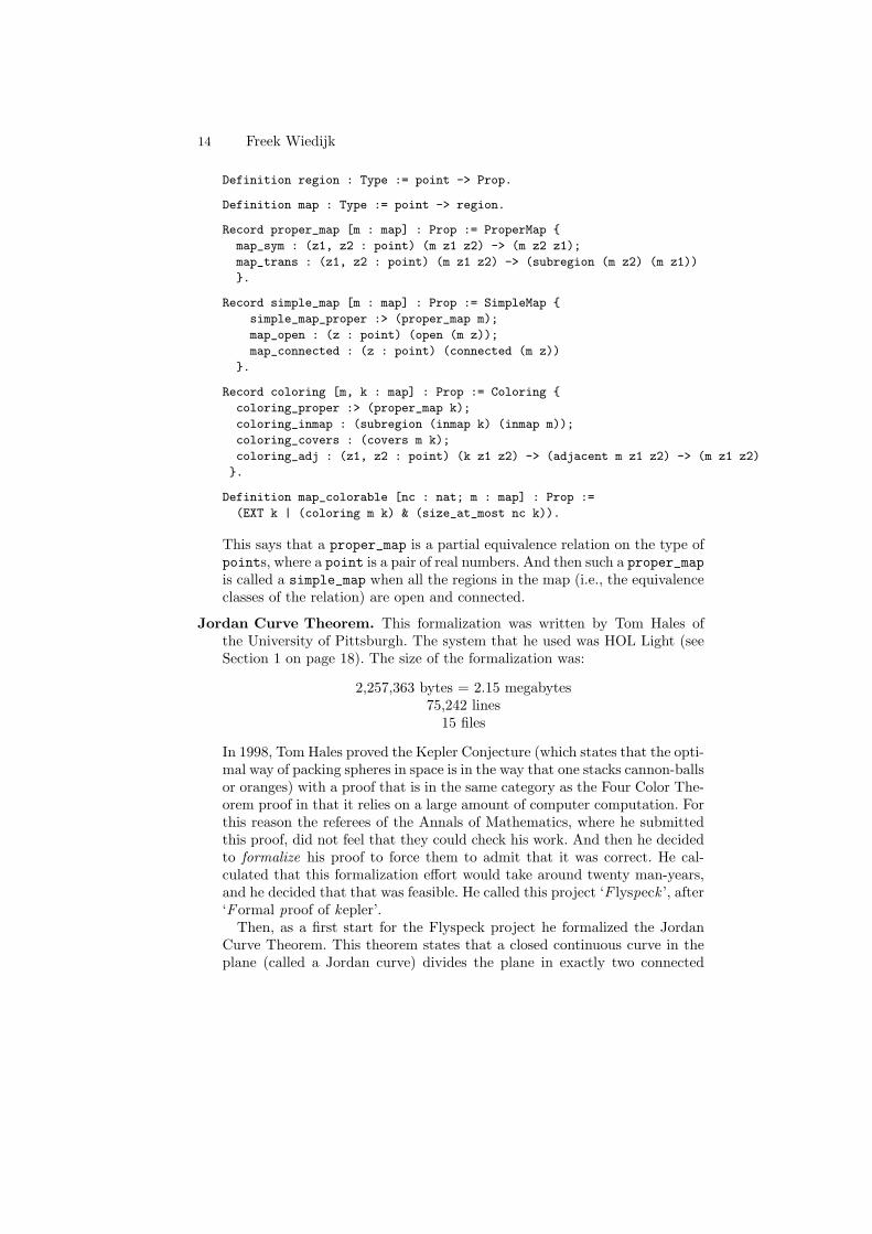
This says that a proper_map is a partial equivalence relation on the type ofpoints, where a point is a pair of real numbers. And then such a proper_mapis called a simple_map when all the regions in the map (i.e., the equivalenceclasses of the relation) are open and connected.
Jordan Curve Theorem. This formalization was written by Tom Hales ofthe University of Pittsburgh. The system that he used was HOL Light (seeSection 1 on page 18). The size of the formalization was:
2,257,363 bytes = 2.15 megabytes75,242 lines
15 files
In 1998, Tom Hales proved the Kepler Conjecture (which states that the opti-mal way of packing spheres in space is in the way that one stacks cannon-ballsor oranges) with a proof that is in the same category as the Four Color The-orem proof in that it relies on a large amount of computer computation. Forthis reason the referees of the Annals of Mathematics, where he submittedthis proof, did not feel that they could check his work. And then he decidedto formalize his proof to force them to admit that it was correct. He cal-culated that this formalization effort would take around twenty man-years,and he decided that that was feasible. He called this project ‘F lyspeck ’, after‘Formal proof of kepler’.
Then, as a first start for the Flyspeck project he formalized the JordanCurve Theorem. This theorem states that a closed continuous curve in theplane (called a Jordan curve) divides the plane in exactly two connected
Introduction 15
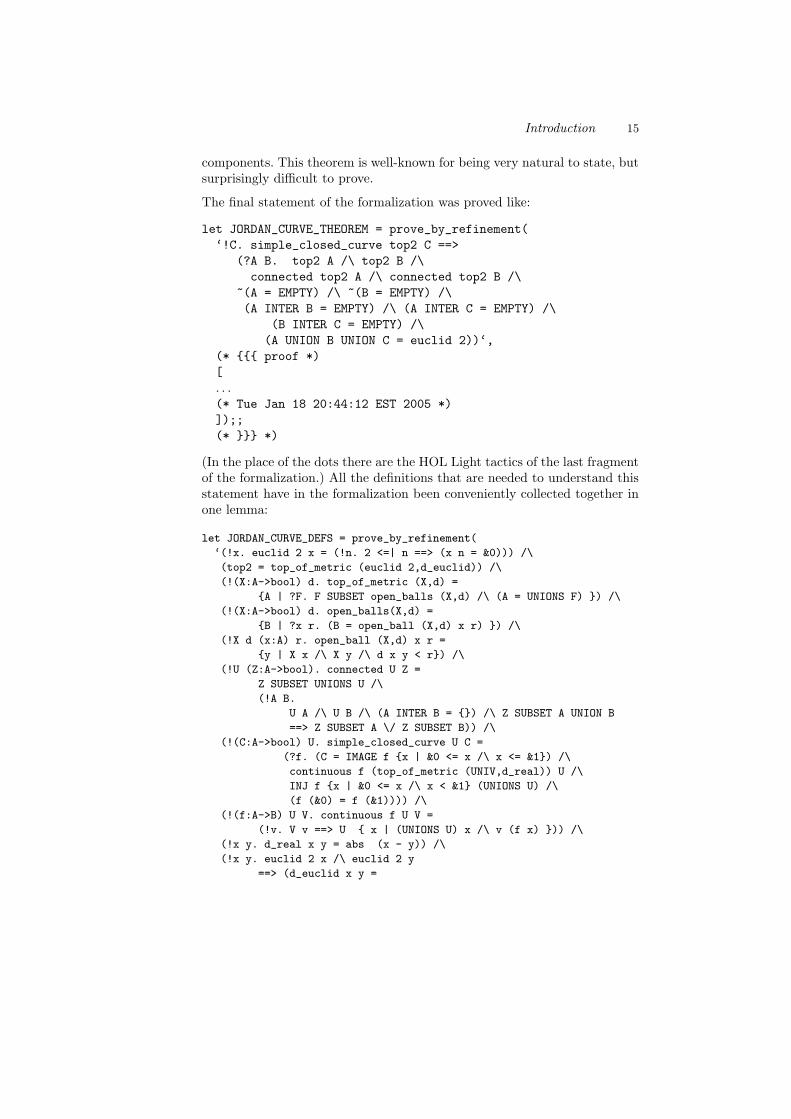
components. This theorem is well-known for being very natural to state, butsurprisingly difficult to prove.
The final statement of the formalization was proved like:
let JORDAN_CURVE_THEOREM = prove_by_refinement(
‘!C. simple_closed_curve top2 C ==>
(?A B. top2 A /\ top2 B /\
connected top2 A /\ connected top2 B /\
~(A = EMPTY) /\ ~(B = EMPTY) /\
(A INTER B = EMPTY) /\ (A INTER C = EMPTY) /\
(B INTER C = EMPTY) /\
(A UNION B UNION C = euclid 2))‘,
(* proof *)
[
. . .(* Tue Jan 18 20:44:12 EST 2005 *)
]);;
(* *)
(In the place of the dots there are the HOL Light tactics of the last fragmentof the formalization.) All the definitions that are needed to understand thisstatement have in the formalization been conveniently collected together inone lemma:
let JORDAN_CURVE_DEFS = prove_by_refinement(
‘(!x. euclid 2 x = (!n. 2 <=| n ==> (x n = &0))) /\
(top2 = top_of_metric (euclid 2,d_euclid)) /\
(!(X:A->bool) d. top_of_metric (X,d) =
A | ?F. F SUBSET open_balls (X,d) /\ (A = UNIONS F) ) /\
(!(X:A->bool) d. open_balls(X,d) =
B | ?x r. (B = open_ball (X,d) x r) ) /\
(!X d (x:A) r. open_ball (X,d) x r =
y | X x /\ X y /\ d x y < r) /\
(!U (Z:A->bool). connected U Z =
Z SUBSET UNIONS U /\
(!A B.
U A /\ U B /\ (A INTER B = ) /\ Z SUBSET A UNION B
==> Z SUBSET A \/ Z SUBSET B)) /\
(!(C:A->bool) U. simple_closed_curve U C =
(?f. (C = IMAGE f x | &0 <= x /\ x <= &1) /\
continuous f (top_of_metric (UNIV,d_real)) U /\
INJ f x | &0 <= x /\ x < &1 (UNIONS U) /\
(f (&0) = f (&1)))) /\
(!(f:A->B) U V. continuous f U V =
(!v. V v ==> U x | (UNIONS U) x /\ v (f x) )) /\
(!x y. d_real x y = abs (x - y)) /\
(!x y. euclid 2 x /\ euclid 2 y
==> (d_euclid x y =

16 Freek Wiedijk
sqrt (sum (0,2) (\i. (x i - y i) * (x i - y i)))))‘,
. . . );;
(All the other notions that occur in these statements are defined in thestandard HOL Light library.)
These three formalizations show that the field of proof assistants is in rapiddevelopment. Theorems that for a long time have seemed to be out of reach ofproof checking technology are now getting their proofs formalized! It is there-fore very exciting to dream about what it will be like when the QED utopia isfinally realized in all its glory. Personally I am convinced that this will happen,eventually. And hopefully this collection of samples from all the provers of theworld will play a small part in bringing this future nearer.
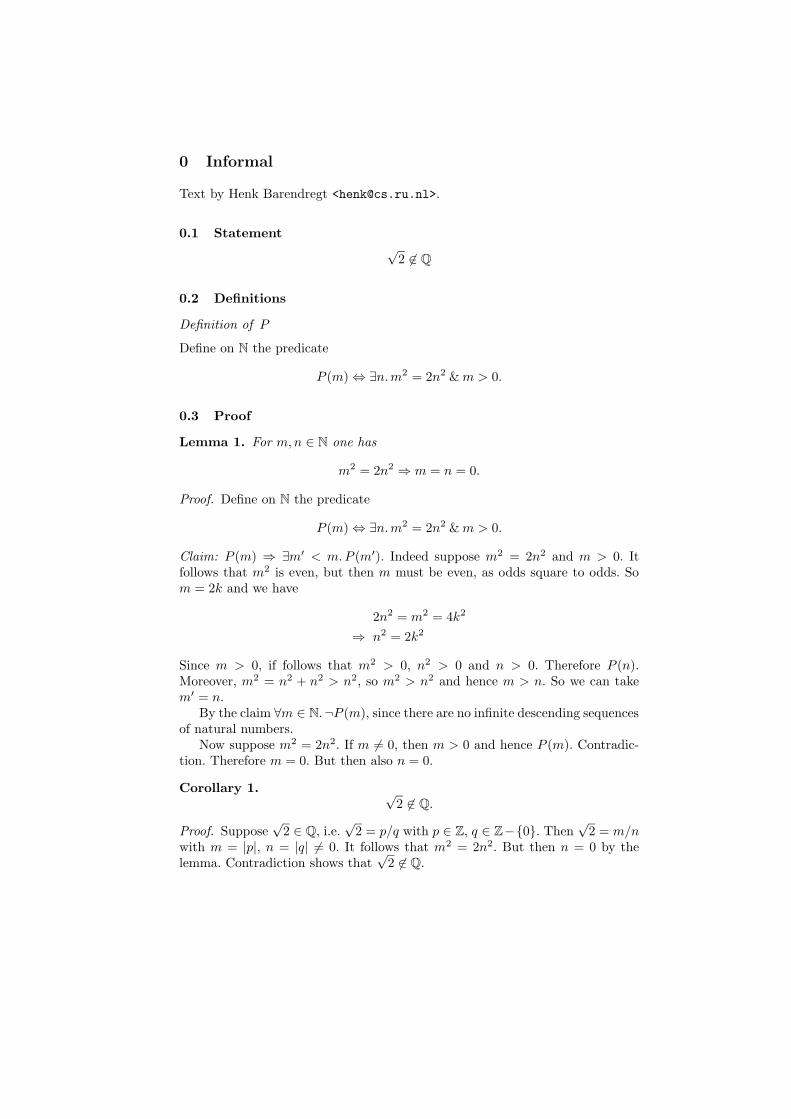
0 Informal
Text by Henk Barendregt <[email protected]>.
0.1 Statement√
2 6∈ Q
0.2 Definitions
Definition of P
Define on N the predicate
P (m) ⇔ ∃n.m2 = 2n2 & m > 0.
0.3 Proof
Lemma 1. For m,n ∈ N one has
m2 = 2n2 ⇒ m = n = 0.
Proof. Define on N the predicate
P (m) ⇔ ∃n.m2 = 2n2 & m > 0.
Claim: P (m) ⇒ ∃m′ < m.P (m′). Indeed suppose m2 = 2n2 and m > 0. Itfollows that m2 is even, but then m must be even, as odds square to odds. Som = 2k and we have
2n2 = m2 = 4k2
⇒ n2 = 2k2
Since m > 0, if follows that m2 > 0, n2 > 0 and n > 0. Therefore P (n).Moreover, m2 = n2 + n2 > n2, so m2 > n2 and hence m > n. So we can takem′ = n.
By the claim ∀m ∈ N.¬P (m), since there are no infinite descending sequencesof natural numbers.
Now suppose m2 = 2n2. If m 6= 0, then m > 0 and hence P (m). Contradic-tion. Therefore m = 0. But then also n = 0.
Corollary 1. √2 6∈ Q.
Proof. Suppose√
2 ∈ Q, i.e.√
2 = p/q with p ∈ Z, q ∈ Z−0. Then√
2 = m/nwith m = |p|, n = |q| 6= 0. It follows that m2 = 2n2. But then n = 0 by thelemma. Contradiction shows that
√2 6∈ Q.
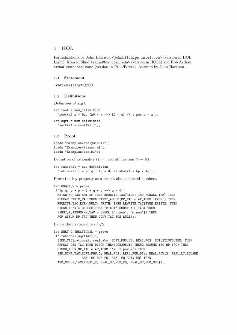
1 HOL
Formalizations by John Harrison <[email protected]> (version in HOLLight), Konrad Slind <[email protected]> (version in HOL4) and Rob Arthan<[email protected]> (version in ProofPower). Answers by John Harrison.
1.1 Statement
~rational(sqrt(&2))
1.2 Definitions
Definition of sqrt
let root = new_definition
‘root(n) x = @u. (&0 < x ==> &0 < u) /\ u pow n = x‘;;
let sqrt = new_definition
‘sqrt(x) = root(2) x‘;;
1.3 Proof
loads "Examples/analysis.ml";;
loads "Examples/transc.ml";;
loads "Examples/sos.ml";;
Definition of rationality (& = natural injection N → R).
let rational = new_definition
‘rational(r) = ?p q. ~(q = 0) /\ abs(r) = &p / &q‘;;
Prove the key property as a lemma about natural numbers.
let NSQRT_2 = prove
(‘!p q. p * p = 2 * q * q ==> q = 0‘,
MATCH_MP_TAC num_WF THEN REWRITE_TAC[RIGHT_IMP_FORALL_THM] THEN
REPEAT STRIP_TAC THEN FIRST_ASSUM(MP_TAC o AP_TERM ‘EVEN‘) THEN
REWRITE_TAC[EVEN_MULT; ARITH] THEN REWRITE_TAC[EVEN_EXISTS] THEN
DISCH_THEN(X_CHOOSE_THEN ‘m:num‘ SUBST_ALL_TAC) THEN
FIRST_X_ASSUM(MP_TAC o SPECL [‘q:num‘; ‘m:num‘]) THEN
POP_ASSUM MP_TAC THEN CONV_TAC SOS_RULE);;
Hence the irrationality of√
2.
let SQRT_2_IRRATIONAL = prove
(‘~rational(sqrt(&2))‘,
SIMP_TAC[rational; real_abs; SQRT_POS_LE; REAL_POS; NOT_EXISTS_THM] THEN
REPEAT GEN_TAC THEN DISCH_THEN(CONJUNCTS_THEN2 ASSUME_TAC MP_TAC) THEN
DISCH_THEN(MP_TAC o AP_TERM ‘\x. x pow 2‘) THEN
ASM_SIMP_TAC[SQRT_POW_2; REAL_POS; REAL_POW_DIV; REAL_POW_2; REAL_LT_SQUARE;
REAL_OF_NUM_EQ; REAL_EQ_RDIV_EQ] THEN
ASM_MESON_TAC[NSQRT_2; REAL_OF_NUM_EQ; REAL_OF_NUM_MUL]);;
HOL 19
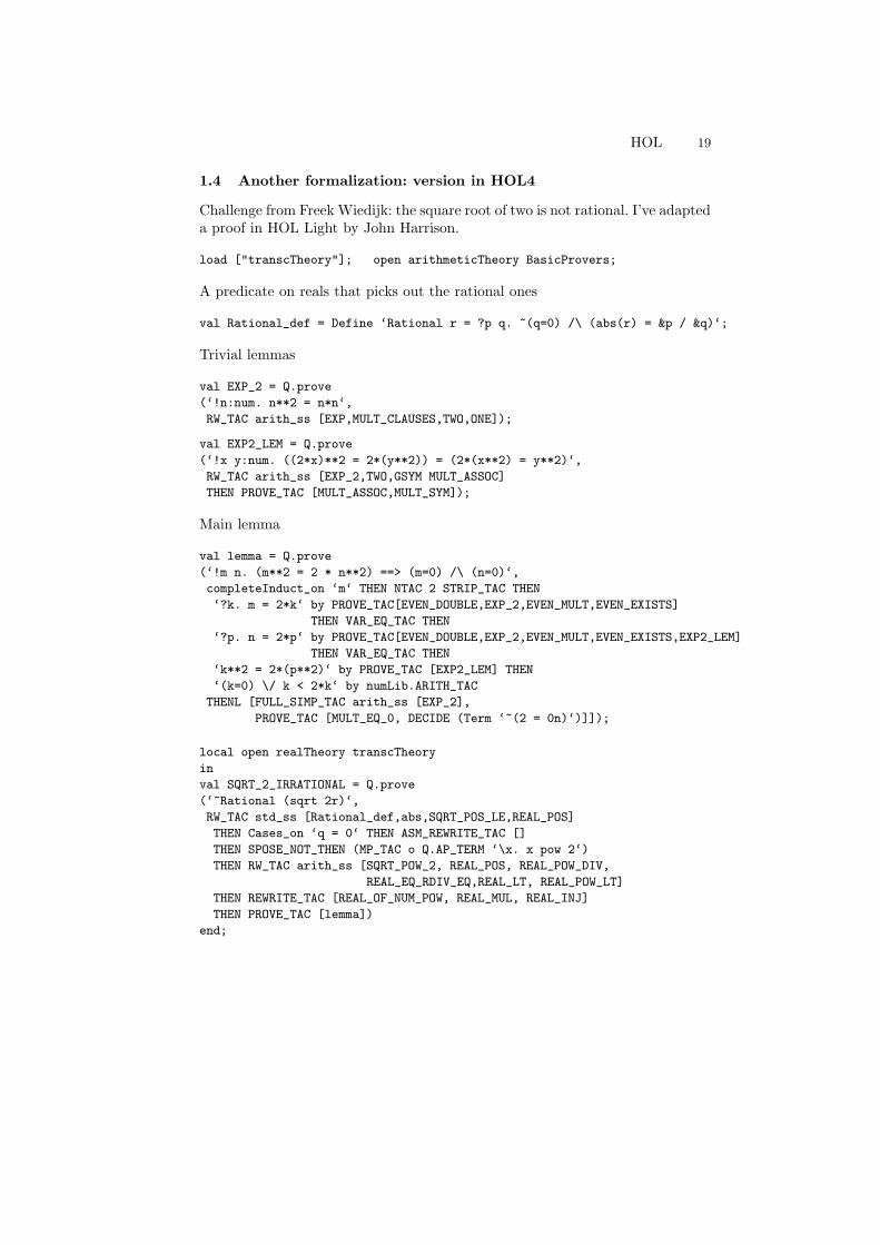
1.4 Another formalization: version in HOL4
Challenge from Freek Wiedijk: the square root of two is not rational. I’ve adapteda proof in HOL Light by John Harrison.
load ["transcTheory"]; open arithmeticTheory BasicProvers;
A predicate on reals that picks out the rational ones
val Rational_def = Define ‘Rational r = ?p q. ~(q=0) /\ (abs(r) = &p / &q)‘;
Trivial lemmas
val EXP_2 = Q.prove
(‘!n:num. n**2 = n*n‘,
RW_TAC arith_ss [EXP,MULT_CLAUSES,TWO,ONE]);
val EXP2_LEM = Q.prove
(‘!x y:num. ((2*x)**2 = 2*(y**2)) = (2*(x**2) = y**2)‘,
RW_TAC arith_ss [EXP_2,TWO,GSYM MULT_ASSOC]
THEN PROVE_TAC [MULT_ASSOC,MULT_SYM]);
Main lemma
val lemma = Q.prove
(‘!m n. (m**2 = 2 * n**2) ==> (m=0) /\ (n=0)‘,
completeInduct_on ‘m‘ THEN NTAC 2 STRIP_TAC THEN
‘?k. m = 2*k‘ by PROVE_TAC[EVEN_DOUBLE,EXP_2,EVEN_MULT,EVEN_EXISTS]
THEN VAR_EQ_TAC THEN
‘?p. n = 2*p‘ by PROVE_TAC[EVEN_DOUBLE,EXP_2,EVEN_MULT,EVEN_EXISTS,EXP2_LEM]
THEN VAR_EQ_TAC THEN
‘k**2 = 2*(p**2)‘ by PROVE_TAC [EXP2_LEM] THEN
‘(k=0) \/ k < 2*k‘ by numLib.ARITH_TAC
THENL [FULL_SIMP_TAC arith_ss [EXP_2],
PROVE_TAC [MULT_EQ_0, DECIDE (Term ‘~(2 = 0n)‘)]]);
local open realTheory transcTheory
in
val SQRT_2_IRRATIONAL = Q.prove
(‘~Rational (sqrt 2r)‘,
RW_TAC std_ss [Rational_def,abs,SQRT_POS_LE,REAL_POS]
THEN Cases_on ‘q = 0‘ THEN ASM_REWRITE_TAC []
THEN SPOSE_NOT_THEN (MP_TAC o Q.AP_TERM ‘\x. x pow 2‘)
THEN RW_TAC arith_ss [SQRT_POW_2, REAL_POS, REAL_POW_DIV,
REAL_EQ_RDIV_EQ,REAL_LT, REAL_POW_LT]
THEN REWRITE_TAC [REAL_OF_NUM_POW, REAL_MUL, REAL_INJ]
THEN PROVE_TAC [lemma])
end;
20 John Harrison, Konrad Slind, Rob Arthan
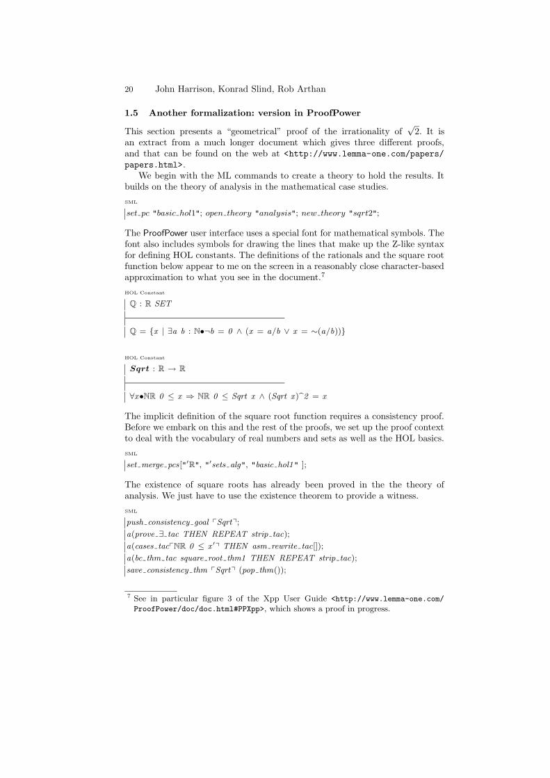
1.5 Another formalization: version in ProofPower
This section presents a “geometrical” proof of the irrationality of√
2. It isan extract from a much longer document which gives three different proofs,and that can be found on the web at <http://www.lemma-one.com/papers/
papers.html>.We begin with the ML commands to create a theory to hold the results. It
builds on the theory of analysis in the mathematical case studies.
SML
set pc "basic hol1"; open theory "analysis"; new theory "sqrt2";
The ProofPower user interface uses a special font for mathematical symbols. Thefont also includes symbols for drawing the lines that make up the Z-like syntaxfor defining HOL constants. The definitions of the rationals and the square rootfunction below appear to me on the screen in a reasonably close character-basedapproximation to what you see in the document.7
HOL Constant
Q : R SET
Q = x | ∃a b : N•¬b = 0 ∧ (x = a/b ∨ x = ∼(a/b))
HOL Constant
Sqrt : R → R
∀x•NR 0 ≤ x ⇒ NR 0 ≤ Sqrt x ∧ (Sqrt x )b2 = x
The implicit definition of the square root function requires a consistency proof.Before we embark on this and the rest of the proofs, we set up the proof contextto deal with the vocabulary of real numbers and sets as well as the HOL basics.
SML
set merge pcs["′R", "′sets alg", "basic hol1" ];
The existence of square roots has already been proved in the the theory ofanalysis. We just have to use the existence theorem to provide a witness.
SML
push consistency goal pSqrtq;
a(prove ∃ tac THEN REPEAT strip tac);
a(cases tacpNR 0 ≤ x ′q THEN asm rewrite tac[]);
a(bc thm tac square root thm1 THEN REPEAT strip tac);
save consistency thm pSqrtq (pop thm());
7 See in particular figure 3 of the Xpp User Guide <http://www.lemma-one.com/
ProofPower/doc/doc.html#PPXpp>, which shows a proof in progress.
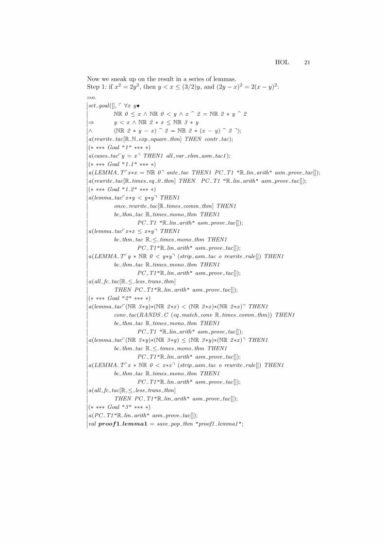
HOL 21
Now we sneak up on the result in a series of lemmas.Step 1: if x2 = 2y2, then y < x ≤ (3/2)y, and (2y − x)2 = 2(x − y)2:
SML
set goal([], p ∀x y•NR 0 ≤ x ∧ NR 0 < y ∧ x b 2 = NR 2 ∗ y b 2
⇒ y < x ∧ NR 2 ∗ x ≤ NR 3 ∗ y
∧ (NR 2 ∗ y − x ) b 2 = NR 2 ∗ (x − y) b 2 q);
a(rewrite tac[R N exp square thm] THEN contr tac);
(∗ ∗∗∗ Goal "1" ∗∗∗ ∗)a(cases tacpy = xq THEN1 all var elim asm tac1 );
(∗ ∗∗∗ Goal "1 .1" ∗∗∗ ∗)a(LEMMA Tpx∗x = NR 0q ante tac THEN1 PC T1 "R lin arith" asm prove tac[]);
a(rewrite tac[R times eq 0 thm] THEN PC T1 "R lin arith" asm prove tac[]);
(∗ ∗∗∗ Goal "1 .2" ∗∗∗ ∗)a(lemma tacpx∗y < y∗yq THEN1
once rewrite tac[R times comm thm] THEN1
bc thm tac R times mono thm THEN1
PC T1 "R lin arith" asm prove tac[]);
a(lemma tacpx∗x ≤ x∗yq THEN1
bc thm tac R ≤ times mono thm THEN1
PC T1"R lin arith" asm prove tac[]);
a(LEMMA Tpy ∗ NR 0 < y∗yq (strip asm tac o rewrite rule[]) THEN1
bc thm tac R times mono thm THEN1
PC T1"R lin arith" asm prove tac[]);
a(all fc tac[R ≤ less trans thm]
THEN PC T1"R lin arith" asm prove tac[]);
(∗ ∗∗∗ Goal "2" ∗∗∗ ∗)a(lemma tacp(NR 3∗y)∗(NR 2∗x ) < (NR 2∗x )∗(NR 2∗x )q THEN1
conv tac(RANDS C (eq match conv R times comm thm)) THEN1
bc thm tac R times mono thm THEN1
PC T1 "R lin arith" asm prove tac[]);
a(lemma tacp(NR 3∗y)∗(NR 3∗y) ≤ (NR 3∗y)∗(NR 2∗x )q THEN1
bc thm tac R ≤ times mono thm THEN1
PC T1"R lin arith" asm prove tac[]);
a(LEMMA Tpx ∗ NR 0 < x∗xq (strip asm tac o rewrite rule[]) THEN1
bc thm tac R times mono thm THEN1
PC T1"R lin arith" asm prove tac[]);
a(all fc tac[R ≤ less trans thm]
THEN PC T1"R lin arith" asm prove tac[]);
(∗ ∗∗∗ Goal "3" ∗∗∗ ∗)a(PC T1"R lin arith" asm prove tac[]);
val proof1 lemma1 = save pop thm "proof1 lemma1";
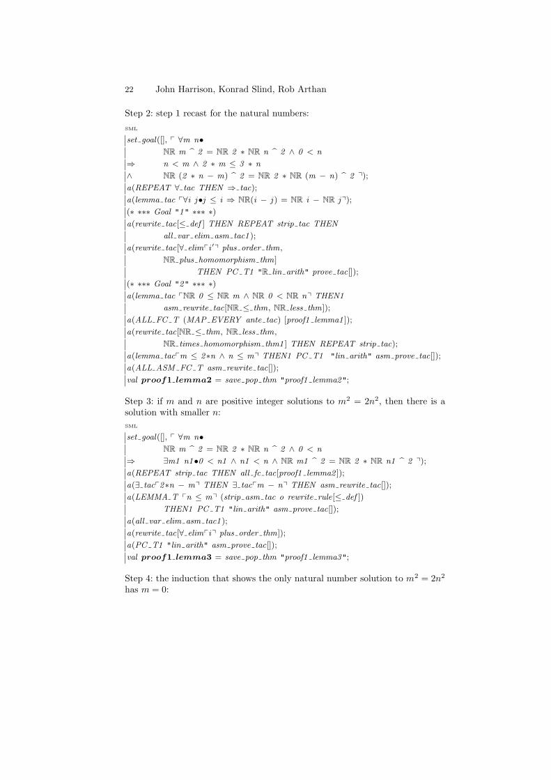
22 John Harrison, Konrad Slind, Rob Arthan
Step 2: step 1 recast for the natural numbers:
SML
set goal([], p ∀m n•NR m b 2 = NR 2 ∗ NR n b 2 ∧ 0 < n
⇒ n < m ∧ 2 ∗ m ≤ 3 ∗ n
∧ NR (2 ∗ n − m) b 2 = NR 2 ∗ NR (m − n) b 2 q);
a(REPEAT ∀ tac THEN ⇒ tac);
a(lemma tac p∀i j•j ≤ i ⇒ NR(i − j ) = NR i − NR jq);
(∗ ∗∗∗ Goal "1" ∗∗∗ ∗)a(rewrite tac[≤ def ] THEN REPEAT strip tac THEN
all var elim asm tac1 );
a(rewrite tac[∀ elimpi ′q plus order thm,
NR plus homomorphism thm]
THEN PC T1 "R lin arith" prove tac[]);
(∗ ∗∗∗ Goal "2" ∗∗∗ ∗)a(lemma tac pNR 0 ≤ NR m ∧ NR 0 < NR nq THEN1
asm rewrite tac[NR ≤ thm, NR less thm]);
a(ALL FC T (MAP EVERY ante tac) [proof1 lemma1 ]);
a(rewrite tac[NR ≤ thm, NR less thm,
NR times homomorphism thm1 ] THEN REPEAT strip tac);
a(lemma tacpm ≤ 2∗n ∧ n ≤ mq THEN1 PC T1 "lin arith" asm prove tac[]);
a(ALL ASM FC T asm rewrite tac[]);
val proof1 lemma2 = save pop thm "proof1 lemma2";
Step 3: if m and n are positive integer solutions to m2 = 2n2, then there is asolution with smaller n:
SML
set goal([], p ∀m n•NR m b 2 = NR 2 ∗ NR n b 2 ∧ 0 < n
⇒ ∃m1 n1•0 < n1 ∧ n1 < n ∧ NR m1 b 2 = NR 2 ∗ NR n1 b 2 q);
a(REPEAT strip tac THEN all fc tac[proof1 lemma2 ]);
a(∃ tacp2∗n − mq THEN ∃ tacpm − nq THEN asm rewrite tac[]);
a(LEMMA T pn ≤ mq (strip asm tac o rewrite rule[≤ def ])
THEN1 PC T1 "lin arith" asm prove tac[]);
a(all var elim asm tac1 );
a(rewrite tac[∀ elimpiq plus order thm]);
a(PC T1 "lin arith" asm prove tac[]);
val proof1 lemma3 = save pop thm "proof1 lemma3";
Step 4: the induction that shows the only natural number solution to m2 = 2n2
has m = 0:
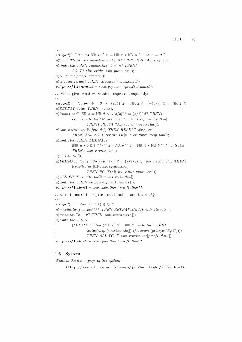
HOL 23
SML
set goal([], p ∀n m• NR m b 2 = NR 2 ∗ NR n b 2 ⇒ n = 0 q);
a(∀ tac THEN cov induction tacpn:Nq THEN REPEAT strip tac);
a(contr tac THEN lemma tac p0 < nq THEN1
PC T1 "lin arith" asm prove tac[]);
a(all fc tac[proof1 lemma3 ]);
a(all asm fc tac[] THEN all var elim asm tac1 );
val proof1 lemma4 = save pop thm "proof1 lemma4";
. . . which gives what we wanted, expressed explicitly:SML
set goal([], p ∀a b• ¬b = 0 ⇒ ¬(a/b)b2 = NR 2 ∧ ¬(∼(a/b)b2 ) = NR 2 q);
a(REPEAT ∀ tac THEN ⇒ tac);
a(lemma tacp¬NR b = NR 0 ∧ ∼(a/b)b2 = (a/b)b2q THEN1
asm rewrite tac[NR one one thm, R N exp square thm]
THEN1 PC T1 "R lin arith" prove tac[]);
a(asm rewrite tac[R frac def ] THEN REPEAT strip tac
THEN ALL FC T rewrite tac[R over times recip thm]);
a(contr tac THEN LEMMA Tp
(NR a ∗ NR b −1 ) b 2 ∗ NR b b 2 = NR 2 ∗ NR b b 2q ante tac
THEN1 asm rewrite tac[]);
a(rewrite tac[]);
a(LEMMA Tp∀x y z :R•(x∗y)b2∗zb2 = (x∗z∗y)b2q rewrite thm tac THEN1
(rewrite tac[R N exp square thm]
THEN PC T1"R lin arith" prove tac[]));
a(ALL FC T rewrite tac[R times recip thm]);
a(contr tac THEN all fc tac[proof1 lemma4 ]);
val proof1 thm1 = save pop thm "proof1 thm1";
. . . or in terms of the square root function and the set Q.SML
set goal([], p ¬Sqrt (NR 2 ) ∈ Q q);
a(rewrite tac[get specpQq] THEN REPEAT UNTIL is ∨ strip tac);
a(cases tac pb = 0q THEN asm rewrite tac[]);
a(contr tac THEN
(LEMMA T pSqrt(NR 2 )b2 = NR 2q ante tac THEN1
bc tac(map (rewrite rule[]) (fc canon (get specpSqrtq))))
THEN ALL FC T asm rewrite tac[proof1 thm1 ]);
val proof1 thm2 = save pop thm "proof1 thm2";
1.6 System
What is the home page of the system?
<http://www.cl.cam.ac.uk/users/jrh/hol-light/index.html>
24 John Harrison, Konrad Slind, Rob Arthan
What are the books about the system? There are no books specifically about theHOL Light system, but it has much in common with ‘HOL88’, described in thefollowing book:
Michael J. C. Gordon and Thomas F. Melham, Introduction to HOL: atheorem proving environment for higher order logic , Cambridge Univer-sity Press, 1993.
and there is a preliminary user manual on the above Web page.
What is the logic of the system? Classical higher-order logic with axioms ofinfinity, extensionality and choice, based on simply typed lambda-calculus withpolymorphic type variables. HOL Light’s core axiomatization is close to the usualdefinition of the internal logic of a topos, and so is intuitionistic in style, butonce the Axiom of Choice in the form of Hilbert’s ε is added, the logic becomesclassical.
What is the implementation architecture of the system? HOL Light follows theLCF approach. The system is built around a ‘logical core’ of primitive inferencerules. Using an abstract type of theorems ensures that theorems can only beconstructed by applying these inference rules. However, these can be composedin arbitrarily sophisticated ways by additional layers of programming.
What does working with the system look like? One normally works inside theread-eval-print loop of the implementation language, Objective CAML. However,since the system is fully programmable, other means of interaction can be, andhave been, written on top.
What is special about the system compared to other systems? HOL Light is prob-ably the system that represents the LCF ideal in its purest form. The primitiverules of the logic are very simple, with the entire logical core including supportfunctions consisting of only 433 lines of OCaml (excluding comments and blanklines). Yet from this foundation some quite powerful decision procedures andnon-trivial mathematical theories are developed, and the system has been usedfor some substantial formal verification projects in industry.
What are other versions of the system?
– HOL88, hol90 and hol98:<http://www.cl.cam.ac.uk/Research/HVG/HOL/HOL.html#getting>
– HOL4:<http://hol.sourceforge.net/>
– ProofPower:<http://www.lemma-one.com/ProofPower/index/index.html>
HOL 25
Who are the people behind the system? HOL Light was almost entirely writtenby John Harrison. However, it builds on earlier versions of HOL, notably theoriginal work by Gordon and Melham and the improved implementation byKonrad Slind, not to mention the earlier work on Edinburgh and CambridgeLCF.
What are the main user communities of the system? HOL Light was originallyan experimental ‘reference’ version of HOL and little active effort was made todevelop a large user community, though it has been used quite extensively insideIntel to formally verify floating-point algorithms. Recently it has attracted moreusers based on its role in the Flyspeck project to formalize the proof by Halesof Kepler’s conjecture:
<http://www.math.pitt.edu/~thales/flyspeck/>
What large mathematical formalizations have been done in the system?
– Analysis: Construction of the real numbers, real analysis up to fundamentaltheorem of calculus, complex numbers up to the fundamental theorem ofalgebra, multivariate calculus up to inverse function theorem.
– Topology: Elementary topological notions, classic theorems about Euclideanspace including Brouwer’s fixpoint theorem and the Jordan curve theorem.
– Logic: classic metatheorems of first order logic (compactness, Lowenheim-Skolem etc.), Tarski’s theorem on the undefinability of truth, Godel’s firstincompleteness theorem.
– Number theory: Basic results on primality and divisibility, weak prime num-ber theorem, Bertrand’s theorem, proof that exponentiation is diophantine.
In addition, many large formal verification proofs, and some of these have usednon-trivial mathematics including series expansions for transcendentals, resultsfrom diophantine approximation and certification of primality, as well as manygeneral results about floating-point rounding.
What representation of the formalization has been put in this paper? A tacticscript in the form of interpreted OCaml source code.
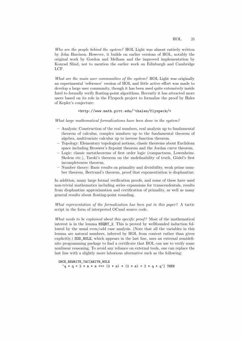
What needs to be explained about this specific proof? Most of the mathematicalinterest is in the lemma NSQRT_2. This is proved by wellfounded induction fol-lowed by the usual even/odd case analysis. (Note that all the variables in thislemma are natural numbers, inferred by HOL from context rather than givenexplicitly.) SOS_RULE, which appears in the last line, uses an external semidefi-nite programming package to find a certificate that HOL can use to verify somenonlinear reasoning. To avoid any reliance on external tools, one can replace thelast line with a slightly more laborious alternative such as the following:
ONCE_REWRITE_TAC[ARITH_RULE
‘q * q = 2 * m * m <=> (2 * m) * (2 * m) = 2 * q * q‘] THEN
26 John Harrison, Konrad Slind, Rob Arthan
ASM_REWRITE_TAC[ARITH_RULE ‘(q < 2 * m ==> m = 0) <=> 2 * m <= q‘] THEN
DISCH_THEN(MP_TAC o MATCH_MP LE_MULT2 o W CONJ) THEN
ASM_REWRITE_TAC[ARITH_RULE ‘2 * x <= x <=> x = 0‘; MULT_EQ_0]);;
The final result is a reduction of the main theorem to that lemma on naturalnumbers using straightforward but rather tedious simplification with a suite ofbasic properties such as 0 ≤ x ⇒ (
√x)2 = x and 0 < z ⇒ (x = y/z ⇔ x · z = y).
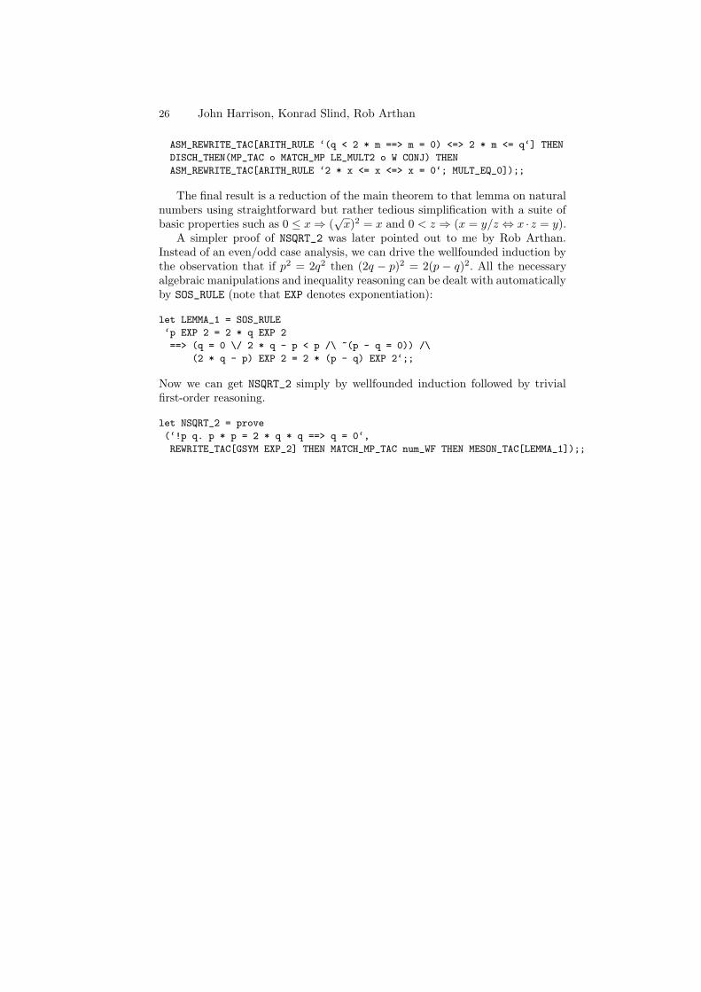
A simpler proof of NSQRT_2 was later pointed out to me by Rob Arthan.Instead of an even/odd case analysis, we can drive the wellfounded induction bythe observation that if p2 = 2q2 then (2q − p)2 = 2(p − q)2. All the necessaryalgebraic manipulations and inequality reasoning can be dealt with automaticallyby SOS_RULE (note that EXP denotes exponentiation):
let LEMMA_1 = SOS_RULE
‘p EXP 2 = 2 * q EXP 2
==> (q = 0 \/ 2 * q - p < p /\ ~(p - q = 0)) /\
(2 * q - p) EXP 2 = 2 * (p - q) EXP 2‘;;
Now we can get NSQRT_2 simply by wellfounded induction followed by trivialfirst-order reasoning.
let NSQRT_2 = prove
(‘!p q. p * p = 2 * q * q ==> q = 0‘,
REWRITE_TAC[GSYM EXP_2] THEN MATCH_MP_TAC num_WF THEN MESON_TAC[LEMMA_1]);;
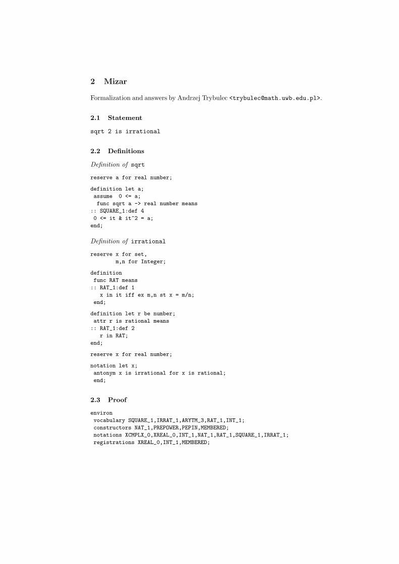
2 Mizar
Formalization and answers by Andrzej Trybulec <[email protected]>.
2.1 Statement
sqrt 2 is irrational
2.2 Definitions
Definition of sqrt
reserve a for real number;
definition let a;
assume 0 <= a;
func sqrt a -> real number means
:: SQUARE_1:def 4
0 <= it & it^2 = a;
end;
Definition of irrational
reserve x for set,
m,n for Integer;
definition
func RAT means
:: RAT_1:def 1
x in it iff ex m,n st x = m/n;
end;
definition let r be number;
attr r is rational means
:: RAT_1:def 2
r in RAT;
end;
reserve x for real number;
notation let x;
antonym x is irrational for x is rational;
end;
2.3 Proof
environ
vocabulary SQUARE_1,IRRAT_1,ARYTM_3,RAT_1,INT_1;
constructors NAT_1,PREPOWER,PEPIN,MEMBERED;
notations XCMPLX_0,XREAL_0,INT_1,NAT_1,RAT_1,SQUARE_1,IRRAT_1;
registrations XREAL_0,INT_1,MEMBERED;
28 Andrzej Trybulec
theorems INT_1,SQUARE_1,REAL_2,INT_2,XCMPLX_1,NAT_1,RAT_1,NEWTON;
requirements ARITHM,REAL,NUMERALS,SUBSET;
begin
theorem
sqrt 2 is irrational
proof
assume sqrt 2 is rational;
then consider i being Integer, n being Nat such that
W1: n<>0 and
W2: sqrt 2=i/n and
W3: for i1 being Integer, n1 being Nat st n1<>0 & sqrt 2=i1/n1 holds n<=n1
by RAT_1:25;
A5: i=sqrt 2*n by W1,XCMPLX_1:88,W2;
C: sqrt 2>=0 & n>0 by W1,NAT_1:19,SQUARE_1:93;
then i>=0 by A5,REAL_2:121;
then reconsider m = i as Nat by INT_1:16;
A6: m*m = n*n*(sqrt 2*sqrt 2) by A5
.= n*n*(sqrt 2)^2 by SQUARE_1:def 3
.= 2*(n*n) by SQUARE_1:def 4;
then 2 divides m*m by NAT_1:def 3;
then 2 divides m by INT_2:44,NEWTON:98;
then consider m1 being Nat such that
W4: m=2*m1 by NAT_1:def 3;
m1*m1*2*2 = m1*(m1*2)*2
.= 2*(n*n) by W4,A6,XCMPLX_1:4;
then 2*(m1*m1) = n*n by XCMPLX_1:5;
then 2 divides n*n by NAT_1:def 3;
then 2 divides n by INT_2:44,NEWTON:98;
then consider n1 being Nat such that
W5: n=2*n1 by NAT_1:def 3;
A10: m1/n1 = sqrt 2 by W4,W5,XCMPLX_1:92,W2;
A11: n1>0 by W5,C,REAL_2:123;
then 2*n1>1*n1 by REAL_2:199;
hence contradiction by A10,W5,A11,W3;
end;
2.4 System
What is the home page of the system?
<http://mizar.org/>
What are the books about the system?
– Bonarska, E., An Introduction to PC Mizar, Fondation Philippe le Hodey,Brussels, 1990.
– Muzalewski, M., An Outline of PC Mizar, Fondation Philippe le Hodey,Brussels, 1993.
– Nakamura, Y. et al., Mizar Lecture Notes (4-th Edition, Mizar Version6.1.12), Shinshu University, Nagano, 2002.
Mizar 29
What is the logic of the system? Mizar is based on classical logic and theJaskowski system of natural deduction (composite logic). It is a formal systemof general applicability, which as such has little in common with any set theory.However, its huge library of formalized mathematical data, Mizar MathematicalLibrary, is based on the Tarski-Grothendieck set theory.
What is the implementation architecture of the system? It is the standard wayof writing compilers – a multipass system consisting of: tokenizer, parser and aseparated grammatical analyzer, as well as logical modules: checker, schematizerand reasoner. The system is coded in Pascal and is currently available for severalplatforms: Microsoft Windows, Intel-based Linux, Solaris and FreeBSD, and alsoDarwin/Mac OS X on PowerPC.
What does working with the system look like? One may call it a ‘lazy interaction’:the article is written in plain ASCII and is processed as whole by the verifier.The best writing technique is the stepwise refinement, where one starts with aproof plan and then fills the gaps reported by the verifier.
What is special about the system compared to other systems? It is easy to use andvery close to the mathematical vernacular. Around 1989 we started the system-atic collection of Mizar articles. Today the Mizar Mathematical Library containsthe impressive number of 900 articles with almost 40000 theorems (about 65 MBof formalized texts).
What are other versions of the system? A very small part of the Mizar language,called Mizar MSE (or sometimes Baby Mizar), has been implemented separately.It can hardly be used for formalizing mathematics, but it has proved to be quiteuseful for teaching and learning logic.
Who are the people behind the system? Andrzej Trybulec is the author of theMizar language, he is also the head of the team implementing the Mizar verifier:
– Grzegorz Bancerek– Czeslaw Bylinski– Adam Grabowski– Artur Kornilowicz– Robert Milewski– Adam Naumowicz– Andrzej Trybulec– Josef Urban
Adam Grabowski is the head of the Library Committee of the Association ofMizar Users (SUM) and is in charge of the Mizar Mathematical Library (MML).
30 Andrzej Trybulec
What are the main user communities of the system? The most active user com-munities are concentrated at University of Bialystok, Poland and Shinshu Uni-versity, Japan. However, more than 160 authors from 10 countries have con-tributed their articles to the Mizar library since its establishing in 1989. Re-cently, we also observe the revival of the (once numerous) community who useMizar for teaching purposes.
What large mathematical formalizations have been done in the system? Thegreatest challenge was the formalizing of the book ‘A Compendium of ContinuousLattices’ by G. Gierz, K. H. Hofmann, K. Keimel, J. D. Lawson, M. Mislove, andD. S. Scott. So far, about 60 per cent of the book’s theory has been covered in theMizar library by 16 Mizar authors. There are also several successful developmentsaimed at formalizing well-known theorems, e.g. Alexander’s Lemma, the BanachFixed Point Theorem for compact spaces, the Brouwer Fixed Point Theorem, theBirkhoff Variety Theorem for manysorted algebras, Fermat’s Little Theorem, theFundamental Theorem of Algebra, the Fundamental Theorem of Arithmetic, theGoedel Completeness Theorem, the Hahn-Banach Theorem for complex and realspaces, the Jordan Curve Theorem for special polygons, the Reflection Theorem,and many others.
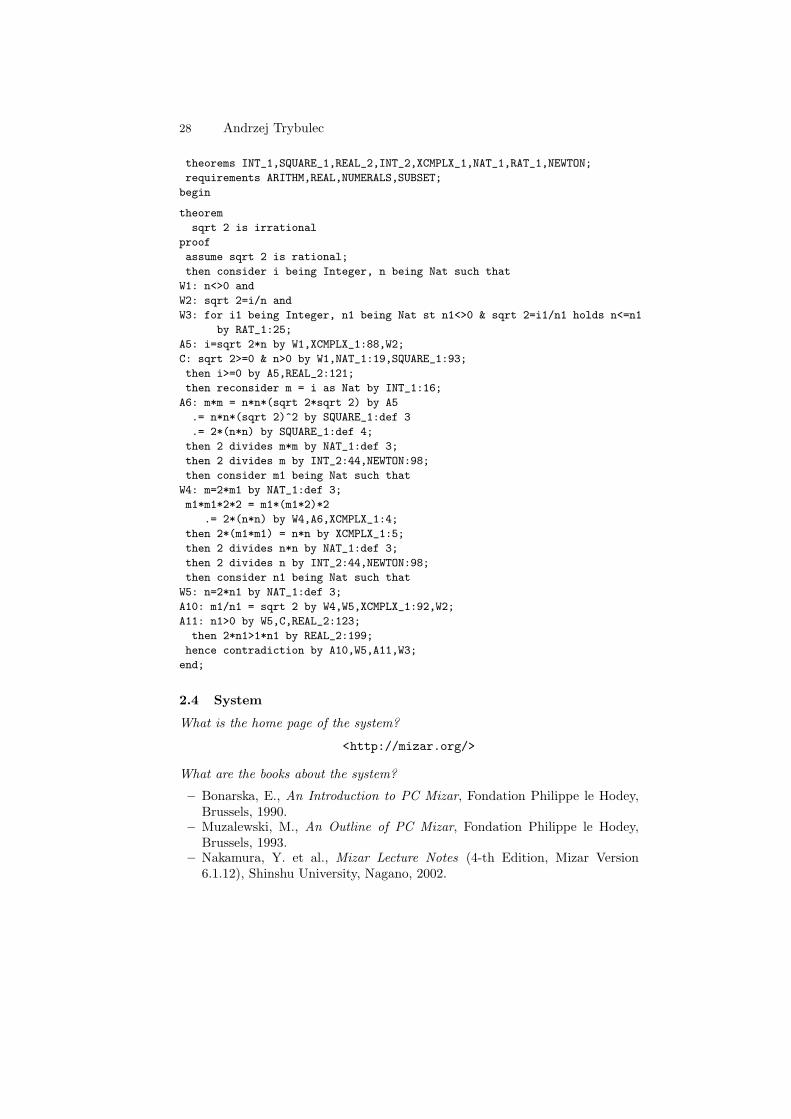
What representation of the formalization has been put in this paper? It is theMizar script, as prepared by the author and checked by the system.
What needs to be explained about this specific proof? The actual proof in Mizarwould now be as follows:
sqtr 2 is irrational by IRRAT_1:1, INT_2:44;
The presented proof is an adjusted version of the proof that the square root ofany prime number is irrational (IRRAT_1:1). So, this is what the proof wouldhave looked like if Freek Wiedijk had not submitted the IRRAT_1 article to theMML in 1999.
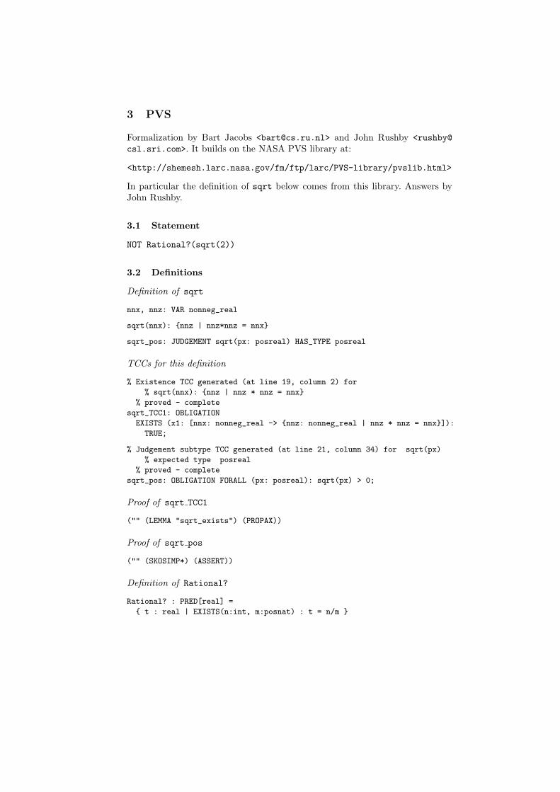
3 PVS
Formalization by Bart Jacobs <[email protected]> and John Rushby <rushby@
csl.sri.com>. It builds on the NASA PVS library at:
<http://shemesh.larc.nasa.gov/fm/ftp/larc/PVS-library/pvslib.html>
In particular the definition of sqrt below comes from this library. Answers byJohn Rushby.
3.1 Statement
NOT Rational?(sqrt(2))
3.2 Definitions
Definition of sqrt
nnx, nnz: VAR nonneg_real
sqrt(nnx): nnz | nnz*nnz = nnx
sqrt_pos: JUDGEMENT sqrt(px: posreal) HAS_TYPE posreal
TCCs for this definition
% Existence TCC generated (at line 19, column 2) for
% sqrt(nnx): nnz | nnz * nnz = nnx
% proved - complete
sqrt_TCC1: OBLIGATION
EXISTS (x1: [nnx: nonneg_real -> nnz: nonneg_real | nnz * nnz = nnx]):
TRUE;
% Judgement subtype TCC generated (at line 21, column 34) for sqrt(px)
% expected type posreal
% proved - complete
sqrt_pos: OBLIGATION FORALL (px: posreal): sqrt(px) > 0;
Proof of sqrt TCC1
("" (LEMMA "sqrt_exists") (PROPAX))
Proof of sqrt pos
("" (SKOSIMP*) (ASSERT))
Definition of Rational?
Rational? : PRED[real] =
t : real | EXISTS(n:int, m:posnat) : t = n/m
32 Bart Jacobs, John Rushby
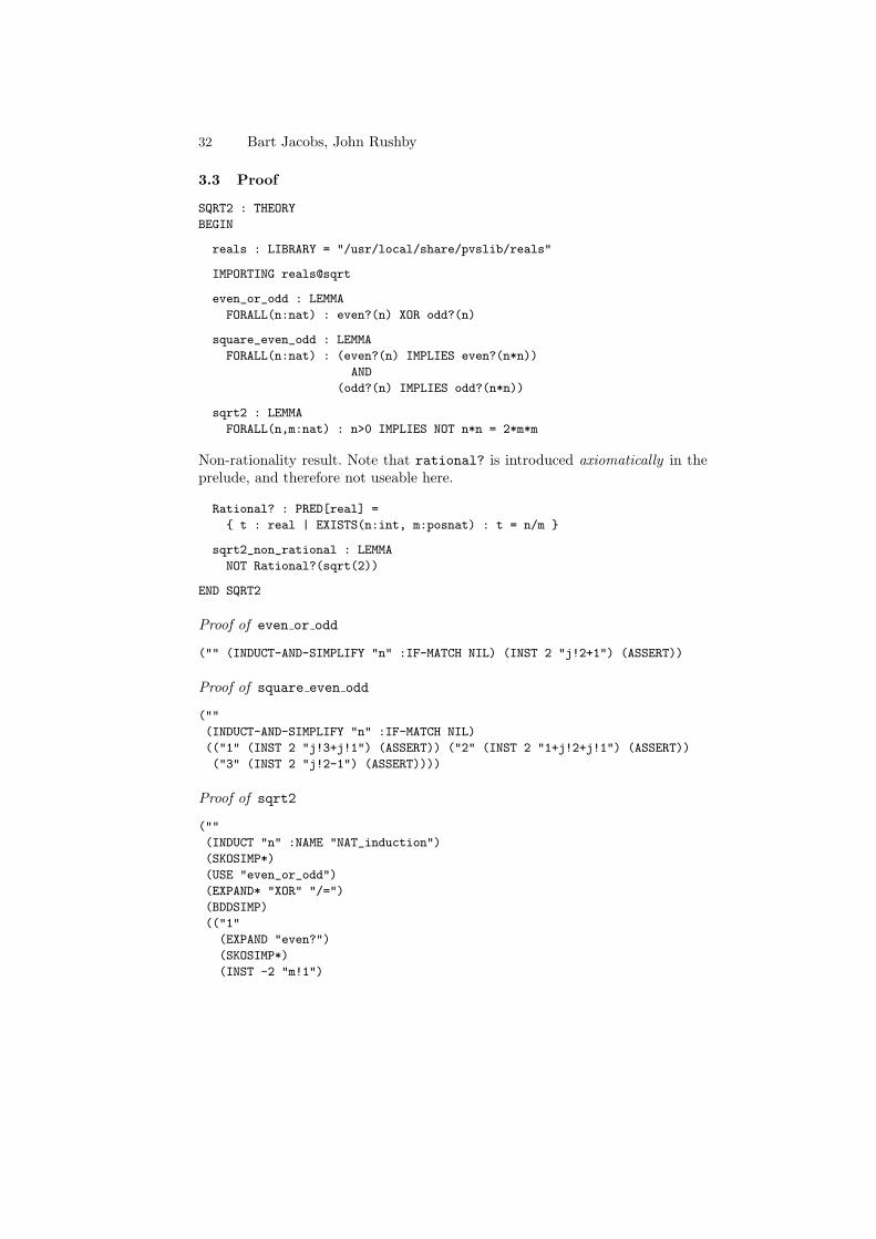
3.3 Proof
SQRT2 : THEORY
BEGIN
reals : LIBRARY = "/usr/local/share/pvslib/reals"
IMPORTING reals@sqrt
even_or_odd : LEMMA
FORALL(n:nat) : even?(n) XOR odd?(n)
square_even_odd : LEMMA
FORALL(n:nat) : (even?(n) IMPLIES even?(n*n))
AND
(odd?(n) IMPLIES odd?(n*n))
sqrt2 : LEMMA
FORALL(n,m:nat) : n>0 IMPLIES NOT n*n = 2*m*m
Non-rationality result. Note that rational? is introduced axiomatically in theprelude, and therefore not useable here.
Rational? : PRED[real] =
t : real | EXISTS(n:int, m:posnat) : t = n/m
sqrt2_non_rational : LEMMA
NOT Rational?(sqrt(2))
END SQRT2
Proof of even or odd
("" (INDUCT-AND-SIMPLIFY "n" :IF-MATCH NIL) (INST 2 "j!2+1") (ASSERT))
Proof of square even odd
(""
(INDUCT-AND-SIMPLIFY "n" :IF-MATCH NIL)
(("1" (INST 2 "j!3+j!1") (ASSERT)) ("2" (INST 2 "1+j!2+j!1") (ASSERT))
("3" (INST 2 "j!2-1") (ASSERT))))
Proof of sqrt2
(""
(INDUCT "n" :NAME "NAT_induction")
(SKOSIMP*)
(USE "even_or_odd")
(EXPAND* "XOR" "/=")
(BDDSIMP)
(("1"
(EXPAND "even?")
(SKOSIMP*)
(INST -2 "m!1")
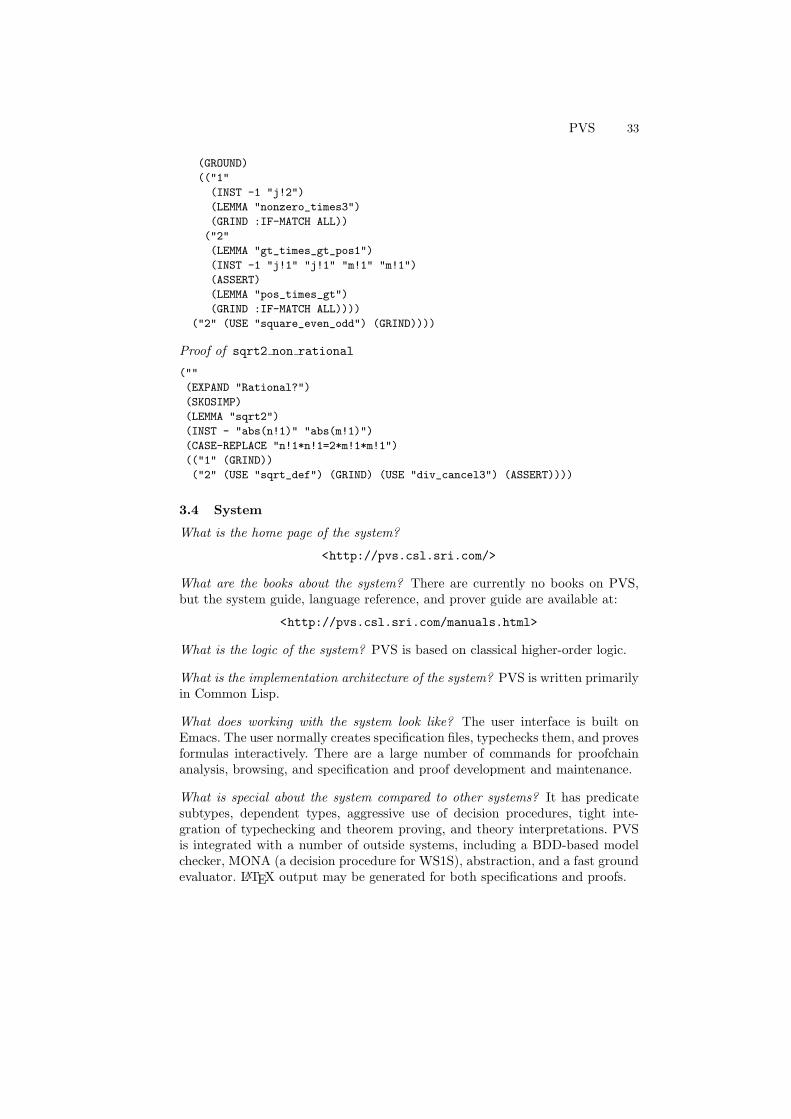
PVS 33
(GROUND)
(("1"
(INST -1 "j!2")
(LEMMA "nonzero_times3")
(GRIND :IF-MATCH ALL))
("2"
(LEMMA "gt_times_gt_pos1")
(INST -1 "j!1" "j!1" "m!1" "m!1")
(ASSERT)
(LEMMA "pos_times_gt")
(GRIND :IF-MATCH ALL))))
("2" (USE "square_even_odd") (GRIND))))
Proof of sqrt2 non rational
(""
(EXPAND "Rational?")
(SKOSIMP)
(LEMMA "sqrt2")
(INST - "abs(n!1)" "abs(m!1)")
(CASE-REPLACE "n!1*n!1=2*m!1*m!1")
(("1" (GRIND))
("2" (USE "sqrt_def") (GRIND) (USE "div_cancel3") (ASSERT))))
3.4 System
What is the home page of the system?
<http://pvs.csl.sri.com/>
What are the books about the system? There are currently no books on PVS,but the system guide, language reference, and prover guide are available at:
<http://pvs.csl.sri.com/manuals.html>
What is the logic of the system? PVS is based on classical higher-order logic.
What is the implementation architecture of the system? PVS is written primarilyin Common Lisp.
What does working with the system look like? The user interface is built onEmacs. The user normally creates specification files, typechecks them, and provesformulas interactively. There are a large number of commands for proofchainanalysis, browsing, and specification and proof development and maintenance.
What is special about the system compared to other systems? It has predicatesubtypes, dependent types, aggressive use of decision procedures, tight inte-gration of typechecking and theorem proving, and theory interpretations. PVSis integrated with a number of outside systems, including a BDD-based modelchecker, MONA (a decision procedure for WS1S), abstraction, and a fast groundevaluator. LATEX output may be generated for both specifications and proofs.
34 Bart Jacobs, John Rushby
What are other versions of the system? The first version of PVS was introducedin 1993. Version 3.0 will be released shortly.
Who are the people behind the system? The formal methods group at SRI:
<http://www.csl.sri.com/programs/formalmethods/>
What are the main user communities of the system? It’s used worldwide in bothacademia and industry – see:
<http://pvs.csl.sri.com/users.html>
What large mathematical formalizations have been done in the system? There isan analysis library, finite sets, domain theory, program semantics, graph theory,set theory, etc.
What representation of the formalization has been put in this paper? This isone of many possible representations in PVS, as functions may be defined ax-iomatically, constructively, or, as in this case, by putting it into the types. Thisparticular representation builds on the definition of sqrt in the reals library atNASA.
What needs to be explained about this specific proof? The TCCs (type-correctnessconditions) are proof obligations generated by the PVS typechecker. Judgementsprovide additional information to the typechecker, so that further TCCs areminimized; in this case after the judgement the typechecker knows that thesqrt of a positive number is positive.
The cited formulas ge_times_ge_pos and nonzero_times3 are from the PVS‘prelude’ (a built-in library of several hundred proven properties outside thescope of PVS decision procedures).
These proofs are the result of an interaction with the PVS prover, whichbuilds a sequent-based proof tree based on commands provided by the user.
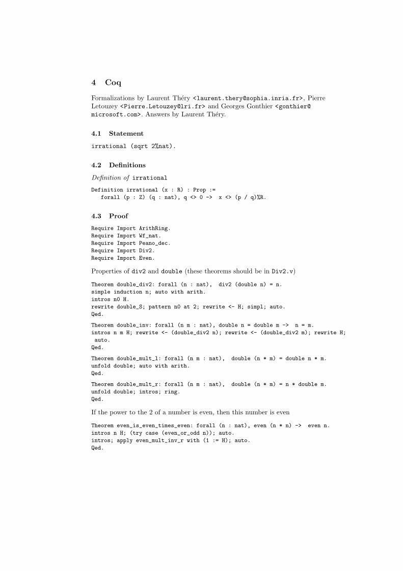
4 Coq
Formalizations by Laurent Thery <[email protected]>, PierreLetouzey <[email protected]> and Georges Gonthier <[email protected]>. Answers by Laurent Thery.
4.1 Statement
irrational (sqrt 2%nat).
4.2 Definitions
Definition of irrational
Definition irrational (x : R) : Prop :=
forall (p : Z) (q : nat), q <> 0 -> x <> (p / q)%R.
4.3 Proof
Require Import ArithRing.
Require Import Wf_nat.
Require Import Peano_dec.
Require Import Div2.
Require Import Even.
Properties of div2 and double (these theorems should be in Div2.v)
Theorem double_div2: forall (n : nat), div2 (double n) = n.
simple induction n; auto with arith.
intros n0 H.
rewrite double_S; pattern n0 at 2; rewrite <- H; simpl; auto.
Qed.
Theorem double_inv: forall (n m : nat), double n = double m -> n = m.
intros n m H; rewrite <- (double_div2 n); rewrite <- (double_div2 m); rewrite H;
auto.
Qed.
Theorem double_mult_l: forall (n m : nat), double (n * m) = double n * m.
unfold double; auto with arith.
Qed.
Theorem double_mult_r: forall (n m : nat), double (n * m) = n * double m.
unfold double; intros; ring.
Qed.
If the power to the 2 of a number is even, then this number is even
Theorem even_is_even_times_even: forall (n : nat), even (n * n) -> even n.
intros n H; (try case (even_or_odd n)); auto.
intros; apply even_mult_inv_r with (1 := H); auto.
Qed.
36 Laurent Thery, Pierre Letouzey, Georges Gonthier
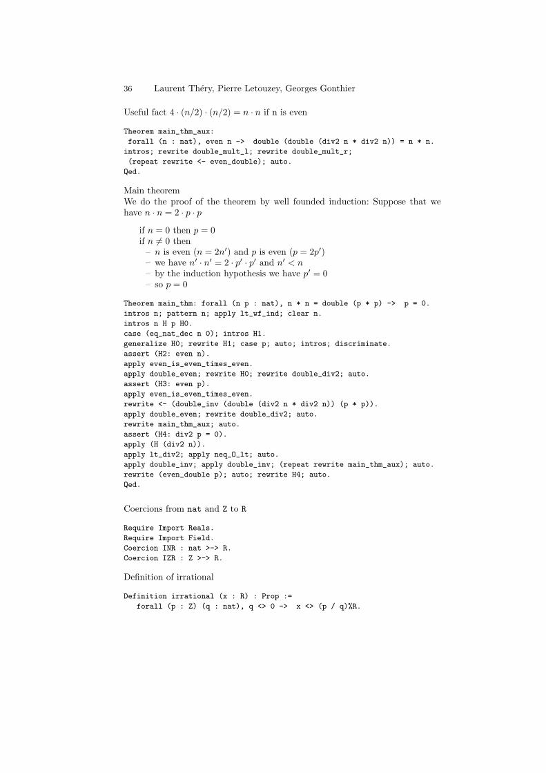
Useful fact 4 · (n/2) · (n/2) = n · n if n is even
Theorem main_thm_aux:
forall (n : nat), even n -> double (double (div2 n * div2 n)) = n * n.
intros; rewrite double_mult_l; rewrite double_mult_r;
(repeat rewrite <- even_double); auto.
Qed.
Main theoremWe do the proof of the theorem by well founded induction: Suppose that wehave n · n = 2 · p · p
if n = 0 then p = 0if n 6= 0 then
– n is even (n = 2n′) and p is even (p = 2p′)– we have n′ · n′ = 2 · p′ · p′ and n′ < n– by the induction hypothesis we have p′ = 0– so p = 0
Theorem main_thm: forall (n p : nat), n * n = double (p * p) -> p = 0.
intros n; pattern n; apply lt_wf_ind; clear n.
intros n H p H0.
case (eq_nat_dec n 0); intros H1.
generalize H0; rewrite H1; case p; auto; intros; discriminate.
assert (H2: even n).
apply even_is_even_times_even.
apply double_even; rewrite H0; rewrite double_div2; auto.
assert (H3: even p).
apply even_is_even_times_even.
rewrite <- (double_inv (double (div2 n * div2 n)) (p * p)).
apply double_even; rewrite double_div2; auto.
rewrite main_thm_aux; auto.
assert (H4: div2 p = 0).
apply (H (div2 n)).
apply lt_div2; apply neq_O_lt; auto.
apply double_inv; apply double_inv; (repeat rewrite main_thm_aux); auto.
rewrite (even_double p); auto; rewrite H4; auto.
Qed.
Coercions from nat and Z to R
Require Import Reals.
Require Import Field.
Coercion INR : nat >-> R.
Coercion IZR : Z >-> R.
Definition of irrational
Definition irrational (x : R) : Prop :=
forall (p : Z) (q : nat), q <> 0 -> x <> (p / q)%R.
Coq 37
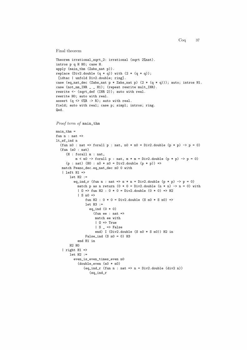
Final theorem
Theorem irrational_sqrt_2: irrational (sqrt 2%nat).
intros p q H H0; case H.
apply (main_thm (Zabs_nat p)).
replace (Div2.double (q * q)) with (2 * (q * q));
[idtac | unfold Div2.double; ring].
case (eq_nat_dec (Zabs_nat p * Zabs_nat p) (2 * (q * q))); auto; intros H1.
case (not_nm_INR _ _ H1); (repeat rewrite mult_INR).
rewrite <- (sqrt_def (INR 2)); auto with real.
rewrite H0; auto with real.
assert (q <> 0%R :> R); auto with real.
field; auto with real; case p; simpl; intros; ring.
Qed.
Proof term of main_thm
main_thm =
fun n : nat =>
lt_wf_ind n
(fun n0 : nat => forall p : nat, n0 * n0 = Div2.double (p * p) -> p = 0)
(fun (n0 : nat)
(H : forall m : nat,
m < n0 -> forall p : nat, m * m = Div2.double (p * p) -> p = 0)
(p : nat) (H0 : n0 * n0 = Div2.double (p * p)) =>
match Peano_dec.eq_nat_dec n0 0 with
| left H1 =>
let H2 :=
eq_ind_r (fun n : nat => n * n = Div2.double (p * p) -> p = 0)
match p as n return (0 * 0 = Div2.double (n * n) -> n = 0) with
| O => fun H2 : 0 * 0 = Div2.double (0 * 0) => H2
| S n0 =>
fun H2 : 0 * 0 = Div2.double (S n0 * S n0) =>
let H3 :=
eq_ind (0 * 0)
(fun ee : nat =>
match ee with
| O => True
| S _ => False
end) I (Div2.double (S n0 * S n0)) H2 in
False_ind (S n0 = 0) H3
end H1 in
H2 H0
| right H1 =>
let H2 :=
even_is_even_times_even n0
(double_even (n0 * n0)
(eq_ind_r (fun n : nat => n = Div2.double (div2 n))
(eq_ind_r
38 Laurent Thery, Pierre Letouzey, Georges Gonthier
(fun n : nat => Div2.double (p * p) = Div2.double n)
(refl_equal (Div2.double (p * p)))
(double_div2 (p * p))) H0)) in
let H3 :=
even_is_even_times_even p
(eq_ind (Div2.double (div2 n0 * div2 n0))
(fun n : nat => even n)
(double_even (Div2.double (div2 n0 * div2 n0))
(eq_ind_r
(fun n : nat =>
Div2.double (div2 n0 * div2 n0) = Div2.double n)
(refl_equal (Div2.double (div2 n0 * div2 n0)))
(double_div2 (div2 n0 * div2 n0))))
(p * p)
(double_inv (Div2.double (div2 n0 * div2 n0))
(p * p)
(eq_ind_r (fun n : nat => n = Div2.double (p * p)) H0
(main_thm_aux n0 H2)))) in
let H4 :=
H (div2 n0) (lt_div2 n0 (neq_O_lt n0 (sym_not_eq H1)))
(div2 p)
(double_inv (div2 n0 * div2 n0) (Div2.double (div2 p * div2 p))
(double_inv (Div2.double (div2 n0 * div2 n0))
(Div2.double (Div2.double (div2 p * div2 p)))
(eq_ind_r
(fun n : nat =>
n =
Div2.double
(Div2.double (Div2.double (div2 p * div2 p))))
(eq_ind_r (fun n : nat => n0 * n0 = Div2.double n) H0
(main_thm_aux p H3)) (main_thm_aux n0 H2)))) in
eq_ind_r (fun p0 : nat => p0 = 0)
(eq_ind_r (fun n1 : nat => Div2.double n1 = 0) (refl_equal 0) H4)
(even_double p H3)
end)
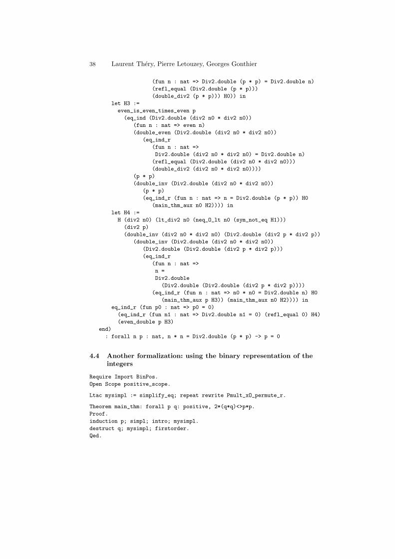
: forall n p : nat, n * n = Div2.double (p * p) -> p = 0
4.4 Another formalization: using the binary representation of theintegers
Require Import BinPos.
Open Scope positive_scope.
Ltac mysimpl := simplify_eq; repeat rewrite Pmult_xO_permute_r.
Theorem main_thm: forall p q: positive, 2*(q*q)<>p*p.
Proof.
induction p; simpl; intro; mysimpl.
destruct q; mysimpl; firstorder.
Qed.
Coq 39
Require Import Reals Field.
Open Scope R_scope.
(* IPR: Injection from Positive to Reals *)
(* Should be in the standard library, close to INR and IZR *)
Definition IPR (p:positive):= (INR (nat_of_P p)).
Coercion IPR : positive >-> R.
Lemma mult_IPR : forall p q, IPR (p * q) = (IPR p * IPR q)%R.
unfold IPR; intros; rewrite nat_of_P_mult_morphism; auto with real.
Qed.
Lemma IPR_eq : forall p q, IPR p = IPR q -> p = q.
unfold IPR; intros; apply nat_of_P_inj; auto with real.
Qed.
Lemma IPR_nonzero : forall p, IPR p <> 0.
unfold IPR; auto with real.
Qed.
Hint Resolve IPR_eq IPR_nonzero.
(* End of IPR *)
Ltac myfield := field; rewrite <- mult_IPR; auto.
Lemma main_thm_pos_rat : forall (p q:positive), 2 <> (p/q)*(p/q).
Proof.
red; intros.
assert (2*(q*q)=p*p).
rewrite H; myfield.
clear H; change 2 with (IPR 2) in H0.
apply main_thm with p q; auto.
repeat rewrite <- mult_IPR in H0; auto.
Qed.
Coercion IZR : Z >-> R.
Lemma main_thm_rat : forall (p:Z)(q:positive), 2 <> (p/q)*(p/q).
Proof.
destruct p; simpl; intros.
replace (0 / q * (0 / q)) with 0.
discrR.
field; rewrite <- mult_IPR; auto.
exact (main_thm_pos_rat p q).
replace (INR (nat_of_P p)) with (IPR p); auto.
replace (- p / q * (- p / q)) with ((p/q)*(p/q)); try myfield.
exact (main_thm_pos_rat p q).
Qed.
Definition irrational (x:R) : Prop := forall (p:Z)(q:positive), x <> (p/q).
Lemma Sqrt2_irr : irrational (sqrt 2).
Proof.
red; intros p q H.
assert (H1: 2 = sqrt 2 * sqrt 2).
symmetry; apply sqrt_sqrt; auto with real.

40 Laurent Thery, Pierre Letouzey, Georges Gonthier
rewrite H in H1; apply main_thm_rat with p q; auto.
Qed.
4.5 Another formalization: Coq in the style of Georges Gonthier
Section Sqrt2.
Variable R : real_model.
Coercion Local fracR := (fracr R).
Theorem sqrt2_irrational : ~(EX f : frac | ‘f = sqrt 2‘).
Proof.
Move=> [f Df]; Step [Hf22 H2f2]: ‘(mulf f f) = F2‘.
Apply: (eqr_trans (fracr_mul ? ? ?)); Apply: eqr_trans (fracrz R (Znat 2)).
By Apply: eqr_trans (square_sqrt (ltrW (ltr02 R))); Apply mulr_morphism.
Step Df2: (eqf F2 (mulf f f)) By Apply/andP; Split; Apply/(fracr_leqPx R ? ?).
Move: f Df2 Hf22 H2f2 Df => [d m]; Rewrite: /eqf /= -eqz_leq; Move/eqP.
Rewrite: scalez_mul -scalez_scale scalez_mul mulzC -1 Zposlock /= -lock.
Step []: (Zpos (S d)) = (scalez d (Znat 1)).
By Apply esym; Apply: eqP; Rewrite scalez_pos; Elim d.
Step [n []]: (EX n | (mulz (Zpos n) (Zpos n)) = (mulz m m)).
Case: m => [n | n]; LeftBy Exists n.
By Exists (S n); Rewrite: -1 (Zneg n)oppz_opp mulz_oppl -mulz_oppr.
Pose i := (addn (S d) n); Move: (leqnn i) m; Rewrite: 1/i.
Elim: i n d => // [i Hrec] n d Hi Dn2; Move/esym: Dn2 Hi.
Rewrite: -nodd_double_half double_addnn !zpos_addn; Move/half: n (odd n) => n.
Case; [Move/((congr oddz) ? ?) | Move/((congr halfz) ? ?)].
By Rewrite: !mulz_addr oddz_add mulzC !mulz_addr oddz_add !oddz_double.
Rewrite: add0n addnC -addnA add0z mulz_addr !halfz_double mulzC mulz_addr.
Case: n => [|n] Dn2 Hi; LeftBy Rewrite: !mulz_nat in Dn2.
Apply: Hrec Dn2; Apply: (leq_trans 3!i) Hi; Apply: leq_addl.
Qed.
End Sqrt2.
4.6 System
What is the home page of the system?
<http://pauillac.inria.fr/coq/>
What are the books about the system? The Coq’Art book
Yves Bertot and Pierre Casteran, Interactive Theorem Proving and Pro-gram Development, Coq’Art: The Calculus of Inductive Constructions,Texts in Theoretical Computer Science. An EATCS Series, 2004, 469pp., ISBN 3-540-20854-2.
provides a pragmatic introduction to the development of proofs and certifiedprograms using Coq. Its web page is:
Coq 41
<http://www.labri.fr/Perso/~casteran/CoqArt/>
Otherwise a reference manual and a tutorial are available at:
<http://pauillac.inria.fr/coq/doc/main.html>
<http://pauillac.inria.fr/coq/doc/tutorial.html>
What is the logic of the system? Coq is based on the Calculus of InductiveConstruction, a lambda calculus with a rich type system with dependent types.
What is the implementation architecture of the system? The system is writtenin ocaml (a dialect of ML). Following Curry-Howard’s isomorphism, the kernelof the system is a type-checking algorithm that checks the correctness of proofs.
What does working with the system look like? The system has a specificationlanguage called Gallina. It allows the user to write its own specification by devel-oping theories. Theories are built from axioms, hypotheses, parameters, lemmas,theorems and definitions of constants, functions, predicates and sets. Proofs areconstructed interactively using the usual LCF tactics approach.
User may interact with the system using the standard shell window but thereare also three available graphical user-interfaces:
– CoqIde an integrated gtk-based user interface– Proof General <http://zermelo.dcs.ed.ac.uk/~proofgen/> an Emacs-
based interface– Pcoq <http://www-sop.inria.fr/lemme/pcoq/> a java-based interface
What is special about the system compared to other systems? First of all, the logicof Coq is very expressive allowing to define rich mathematical objects. Second,Coq manipulates explicit proof objects. A consequence is that the integrity of thesystem only relies on the correct implementation of a typechecking algorithm.Finally, a program extractor synthesizes computer programs obeying their formalspecifications written as logical assertions in the language.
What are other versions of the system? There is only one supported implemen-tation of the system. The current version is 8.0.
Who are the people behind the system? The main developers of the system arefrom the Logical group at INRIA France (<http://logical.inria.fr/>).
What are the main user communities of the system? The main user communitiesare in France (INRIA, LIX, ENS, LRI) and in Holland (Nijmegen).
42 Laurent Thery, Pierre Letouzey, Georges Gonthier
What large mathematical formalizations have been done in the system? The usercontributions are listed at the following address:
http://pauillac.inria.fr/coq/contribs-eng.html.
Here are some relevant ones:
– A proof of the four colour theorem by Georges Gonthier, in collaborationwith Benjamin Werner
– Constructive Category Theory by Amokrane Saıbi– Rational Numbers represented as Stern-Brocot Trees by Milad Niqui– Elements of Constructive Geometry, Group Theory, and Domain Theory by
Gilles Kahn– High School Geometry and Oriented Angles of Vectors in the Plane by
Frederique Guilhot– Basics notions of algebra by Loıc Pottier– Fundamental Theorem of Algebra by Herman Geuvers, Freek Wiedijk, Jan
Zwanenburg, Randy Pollack, Henk Barendregt– Proof of Buchberger’s algorithm by Laurent Thery, Henrik Persson– Rem Theorem in Baire space by Henk Barendregt– Real analysis by Micaela Mayero (standard library)– A Proof of the Three Gap Theorem (Steinhaus Conjecture) by Micaela
Mayero
What representation of the formalization has been put in this paper? What ispresented is the exact script one has to feed Coq with so it accepts the finaltheorem.
After the script a proof term of one of the lemmas is shown.
What needs to be explained about this specific proof? In this proof we havedecided to use as much as possible the notions that were already present inthe system. The predicates even and odd are mutually defined in the theoryEven. The function div2 and double are defined in Div2. The key point of themain proof (main thm) is the application of the well founded induction lt wf ind(second line of the script) whose statement is:
∀p, P . (∀n. (∀m.m < n → (P m)) → (Pn)) → (P p)
The reals are defined in the standard library Reals.
What needs to be explained about the second proof? The second formalization hasbeen inspired by the Minlog entry (page 163). It takes advantage of the positivedatatype of Coq, that encodes strictly positive numbers in a binary way. Thisallows to easily check whether a number is even or not, and also to stick tonormal induction instead of well-founded induction.
Coq 43
What needs to be explained about the third proof? This formalization uses afew basic libraries of the Colour Theorem proof, including a construction of theclassic reals, which has been extended with a definition of the square root (notshown). The type frac is the representation of the rational numbers used in theconstruction of the real numbers.
The proof script uses the extended Coq v7 tactics developed for the FourColour Theorem proof. It is self-contained: the first four lines reduce the problemfrom R to Q, the next two from Q Z, the next five from Z to N, the next twolines set up an induction on the size of the fraction, which is completed in thelast six lines.
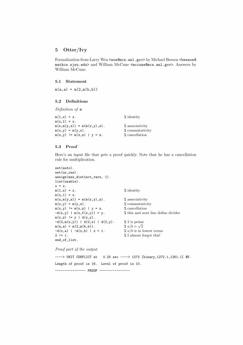
5 Otter/Ivy
Formalization from Larry Wos <[email protected]> by Michael Beeson <beeson@
mathcs.sjsu.edu> and William McCune <[email protected]>. Answers byWilliam McCune.
5.1 Statement
m(a,a) = m(2,m(b,b))
5.2 Definitions
Definition of m
m(1,x) = x. % identitym(x,1) = x.
m(x,m(y,z)) = m(m(x,y),z). % associativitym(x,y) = m(y,x). % commutativitym(x,y) != m(x,z) | y = z. % cancellation
5.3 Proof
Here’s an input file that gets a proof quickly. Note that he has a cancellationrule for multiplication.
set(auto).
set(ur_res).
assign(max_distinct_vars, 1).
list(usable).
x = x.
m(1,x) = x. % identitym(x,1) = x.
m(x,m(y,z)) = m(m(x,y),z). % associativitym(x,y) = m(y,x). % commutativitym(x,y) != m(x,z) | y = z. % cancellation-d(x,y) | m(x,f(x,y)) = y. % this and next line define dividesm(x,z) != y | d(x,y).
-d(2,m(x,y)) | d(2,x) | d(2,y). % 2 is primem(a,a) = m(2,m(b,b)). % a/b =
√2
-d(x,a) | -d(x,b) | x = 1. % a/b is in lowest terms2 != 1. % I almost forgot this!end_of_list.
Proof part of the output
----> UNIT CONFLICT at 0.25 sec ----> 1273 [binary,1272.1,1261.1] $F.
Length of proof is 16. Level of proof is 10.
---------------- PROOF ----------------
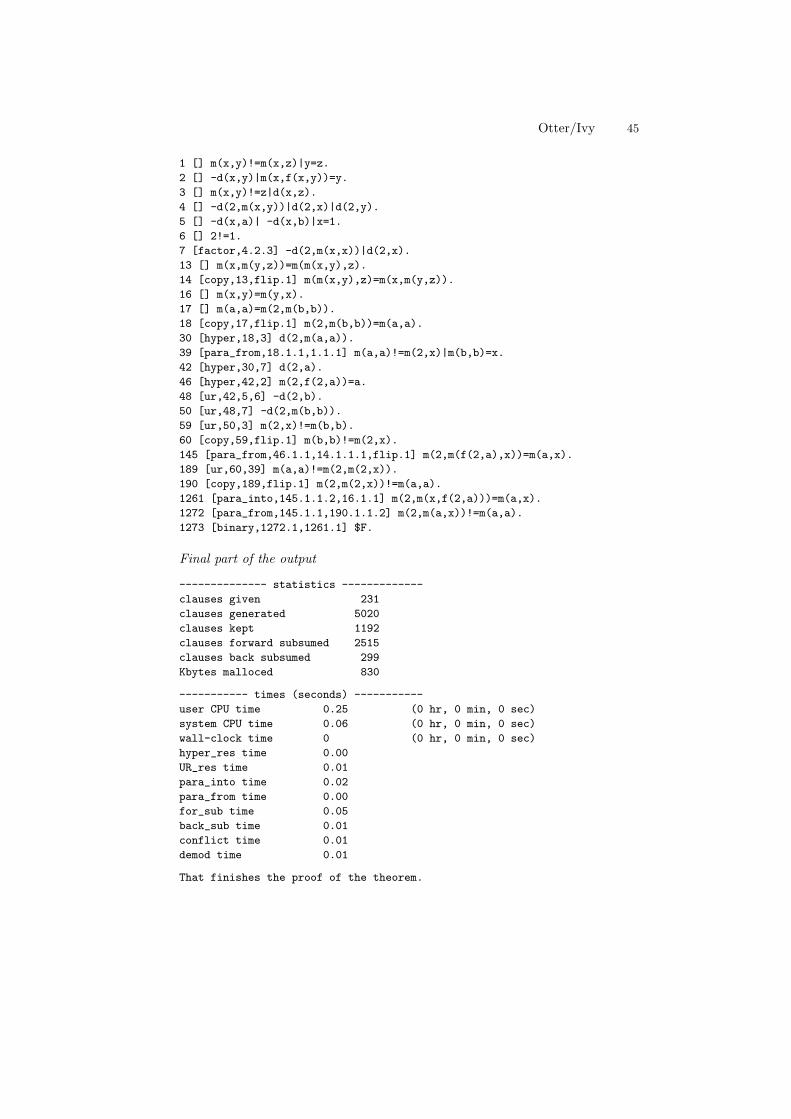
Otter/Ivy 45
1 [] m(x,y)!=m(x,z)|y=z.
2 [] -d(x,y)|m(x,f(x,y))=y.
3 [] m(x,y)!=z|d(x,z).
4 [] -d(2,m(x,y))|d(2,x)|d(2,y).
5 [] -d(x,a)| -d(x,b)|x=1.
6 [] 2!=1.
7 [factor,4.2.3] -d(2,m(x,x))|d(2,x).
13 [] m(x,m(y,z))=m(m(x,y),z).
14 [copy,13,flip.1] m(m(x,y),z)=m(x,m(y,z)).
16 [] m(x,y)=m(y,x).
17 [] m(a,a)=m(2,m(b,b)).
18 [copy,17,flip.1] m(2,m(b,b))=m(a,a).
30 [hyper,18,3] d(2,m(a,a)).
39 [para_from,18.1.1,1.1.1] m(a,a)!=m(2,x)|m(b,b)=x.
42 [hyper,30,7] d(2,a).
46 [hyper,42,2] m(2,f(2,a))=a.
48 [ur,42,5,6] -d(2,b).
50 [ur,48,7] -d(2,m(b,b)).
59 [ur,50,3] m(2,x)!=m(b,b).
60 [copy,59,flip.1] m(b,b)!=m(2,x).
145 [para_from,46.1.1,14.1.1.1,flip.1] m(2,m(f(2,a),x))=m(a,x).
189 [ur,60,39] m(a,a)!=m(2,m(2,x)).
190 [copy,189,flip.1] m(2,m(2,x))!=m(a,a).
1261 [para_into,145.1.1.2,16.1.1] m(2,m(x,f(2,a)))=m(a,x).
1272 [para_from,145.1.1,190.1.1.2] m(2,m(a,x))!=m(a,a).
1273 [binary,1272.1,1261.1] $F.
Final part of the output
-------------- statistics -------------
clauses given 231
clauses generated 5020
clauses kept 1192
clauses forward subsumed 2515
clauses back subsumed 299
Kbytes malloced 830
----------- times (seconds) -----------
user CPU time 0.25 (0 hr, 0 min, 0 sec)
system CPU time 0.06 (0 hr, 0 min, 0 sec)
wall-clock time 0 (0 hr, 0 min, 0 sec)
hyper_res time 0.00
UR_res time 0.01
para_into time 0.02
para_from time 0.00
for_sub time 0.05
back_sub time 0.01
conflict time 0.01
demod time 0.01
That finishes the proof of the theorem.
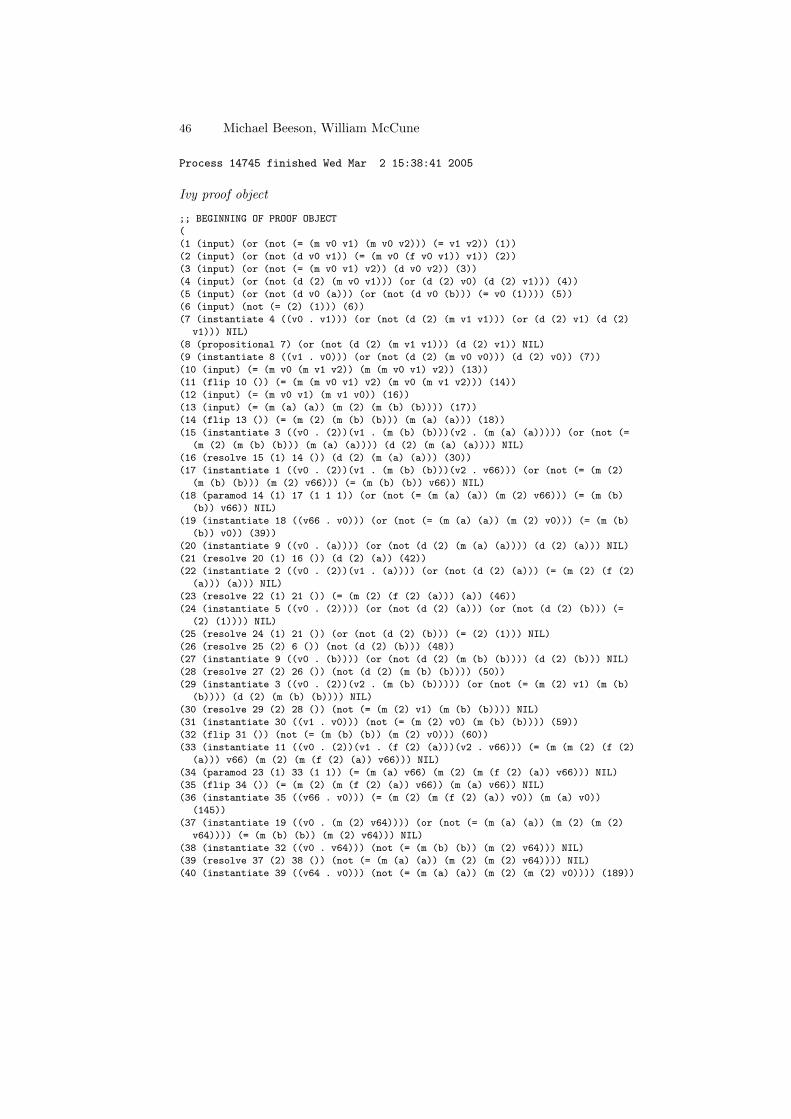
46 Michael Beeson, William McCune
Process 14745 finished Wed Mar 2 15:38:41 2005
Ivy proof object
;; BEGINNING OF PROOF OBJECT
(
(1 (input) (or (not (= (m v0 v1) (m v0 v2))) (= v1 v2)) (1))
(2 (input) (or (not (d v0 v1)) (= (m v0 (f v0 v1)) v1)) (2))
(3 (input) (or (not (= (m v0 v1) v2)) (d v0 v2)) (3))
(4 (input) (or (not (d (2) (m v0 v1))) (or (d (2) v0) (d (2) v1))) (4))
(5 (input) (or (not (d v0 (a))) (or (not (d v0 (b))) (= v0 (1)))) (5))
(6 (input) (not (= (2) (1))) (6))
(7 (instantiate 4 ((v0 . v1))) (or (not (d (2) (m v1 v1))) (or (d (2) v1) (d (2)
v1))) NIL)
(8 (propositional 7) (or (not (d (2) (m v1 v1))) (d (2) v1)) NIL)
(9 (instantiate 8 ((v1 . v0))) (or (not (d (2) (m v0 v0))) (d (2) v0)) (7))
(10 (input) (= (m v0 (m v1 v2)) (m (m v0 v1) v2)) (13))
(11 (flip 10 ()) (= (m (m v0 v1) v2) (m v0 (m v1 v2))) (14))
(12 (input) (= (m v0 v1) (m v1 v0)) (16))
(13 (input) (= (m (a) (a)) (m (2) (m (b) (b)))) (17))
(14 (flip 13 ()) (= (m (2) (m (b) (b))) (m (a) (a))) (18))
(15 (instantiate 3 ((v0 . (2))(v1 . (m (b) (b)))(v2 . (m (a) (a))))) (or (not (=
(m (2) (m (b) (b))) (m (a) (a)))) (d (2) (m (a) (a)))) NIL)
(16 (resolve 15 (1) 14 ()) (d (2) (m (a) (a))) (30))
(17 (instantiate 1 ((v0 . (2))(v1 . (m (b) (b)))(v2 . v66))) (or (not (= (m (2)
(m (b) (b))) (m (2) v66))) (= (m (b) (b)) v66)) NIL)
(18 (paramod 14 (1) 17 (1 1 1)) (or (not (= (m (a) (a)) (m (2) v66))) (= (m (b)
(b)) v66)) NIL)
(19 (instantiate 18 ((v66 . v0))) (or (not (= (m (a) (a)) (m (2) v0))) (= (m (b)
(b)) v0)) (39))
(20 (instantiate 9 ((v0 . (a)))) (or (not (d (2) (m (a) (a)))) (d (2) (a))) NIL)
(21 (resolve 20 (1) 16 ()) (d (2) (a)) (42))
(22 (instantiate 2 ((v0 . (2))(v1 . (a)))) (or (not (d (2) (a))) (= (m (2) (f (2)
(a))) (a))) NIL)
(23 (resolve 22 (1) 21 ()) (= (m (2) (f (2) (a))) (a)) (46))
(24 (instantiate 5 ((v0 . (2)))) (or (not (d (2) (a))) (or (not (d (2) (b))) (=
(2) (1)))) NIL)
(25 (resolve 24 (1) 21 ()) (or (not (d (2) (b))) (= (2) (1))) NIL)
(26 (resolve 25 (2) 6 ()) (not (d (2) (b))) (48))
(27 (instantiate 9 ((v0 . (b)))) (or (not (d (2) (m (b) (b)))) (d (2) (b))) NIL)
(28 (resolve 27 (2) 26 ()) (not (d (2) (m (b) (b)))) (50))
(29 (instantiate 3 ((v0 . (2))(v2 . (m (b) (b))))) (or (not (= (m (2) v1) (m (b)
(b)))) (d (2) (m (b) (b)))) NIL)
(30 (resolve 29 (2) 28 ()) (not (= (m (2) v1) (m (b) (b)))) NIL)
(31 (instantiate 30 ((v1 . v0))) (not (= (m (2) v0) (m (b) (b)))) (59))
(32 (flip 31 ()) (not (= (m (b) (b)) (m (2) v0))) (60))
(33 (instantiate 11 ((v0 . (2))(v1 . (f (2) (a)))(v2 . v66))) (= (m (m (2) (f (2)
(a))) v66) (m (2) (m (f (2) (a)) v66))) NIL)
(34 (paramod 23 (1) 33 (1 1)) (= (m (a) v66) (m (2) (m (f (2) (a)) v66))) NIL)
(35 (flip 34 ()) (= (m (2) (m (f (2) (a)) v66)) (m (a) v66)) NIL)
(36 (instantiate 35 ((v66 . v0))) (= (m (2) (m (f (2) (a)) v0)) (m (a) v0))
(145))
(37 (instantiate 19 ((v0 . (m (2) v64)))) (or (not (= (m (a) (a)) (m (2) (m (2)
v64)))) (= (m (b) (b)) (m (2) v64))) NIL)
(38 (instantiate 32 ((v0 . v64))) (not (= (m (b) (b)) (m (2) v64))) NIL)
(39 (resolve 37 (2) 38 ()) (not (= (m (a) (a)) (m (2) (m (2) v64)))) NIL)
(40 (instantiate 39 ((v64 . v0))) (not (= (m (a) (a)) (m (2) (m (2) v0)))) (189))
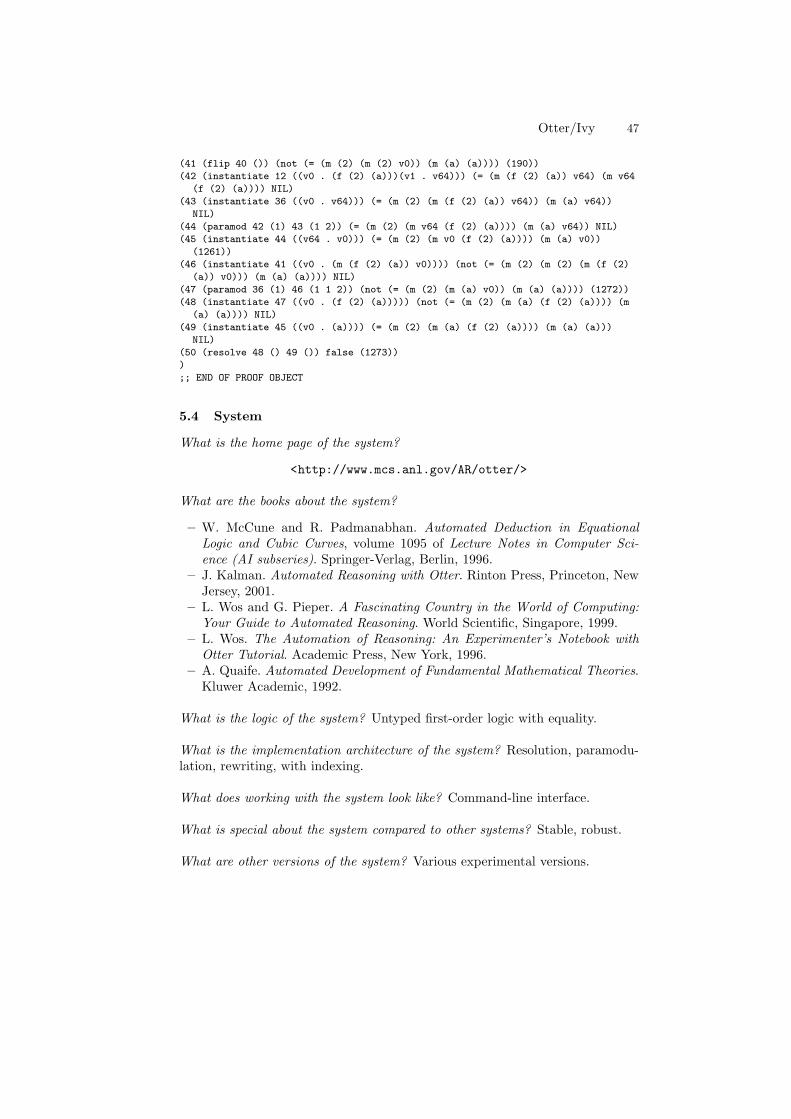
Otter/Ivy 47
(41 (flip 40 ()) (not (= (m (2) (m (2) v0)) (m (a) (a)))) (190))
(42 (instantiate 12 ((v0 . (f (2) (a)))(v1 . v64))) (= (m (f (2) (a)) v64) (m v64
(f (2) (a)))) NIL)
(43 (instantiate 36 ((v0 . v64))) (= (m (2) (m (f (2) (a)) v64)) (m (a) v64))
NIL)
(44 (paramod 42 (1) 43 (1 2)) (= (m (2) (m v64 (f (2) (a)))) (m (a) v64)) NIL)
(45 (instantiate 44 ((v64 . v0))) (= (m (2) (m v0 (f (2) (a)))) (m (a) v0))
(1261))
(46 (instantiate 41 ((v0 . (m (f (2) (a)) v0)))) (not (= (m (2) (m (2) (m (f (2)
(a)) v0))) (m (a) (a)))) NIL)
(47 (paramod 36 (1) 46 (1 1 2)) (not (= (m (2) (m (a) v0)) (m (a) (a)))) (1272))
(48 (instantiate 47 ((v0 . (f (2) (a))))) (not (= (m (2) (m (a) (f (2) (a)))) (m
(a) (a)))) NIL)
(49 (instantiate 45 ((v0 . (a)))) (= (m (2) (m (a) (f (2) (a)))) (m (a) (a)))
NIL)
(50 (resolve 48 () 49 ()) false (1273))
)
;; END OF PROOF OBJECT
5.4 System
What is the home page of the system?
<http://www.mcs.anl.gov/AR/otter/>
What are the books about the system?
– W. McCune and R. Padmanabhan. Automated Deduction in EquationalLogic and Cubic Curves, volume 1095 of Lecture Notes in Computer Sci-ence (AI subseries). Springer-Verlag, Berlin, 1996.
– J. Kalman. Automated Reasoning with Otter. Rinton Press, Princeton, NewJersey, 2001.
– L. Wos and G. Pieper. A Fascinating Country in the World of Computing:Your Guide to Automated Reasoning. World Scientific, Singapore, 1999.
– L. Wos. The Automation of Reasoning: An Experimenter’s Notebook withOtter Tutorial. Academic Press, New York, 1996.
– A. Quaife. Automated Development of Fundamental Mathematical Theories.Kluwer Academic, 1992.
What is the logic of the system? Untyped first-order logic with equality.
What is the implementation architecture of the system? Resolution, paramodu-lation, rewriting, with indexing.
What does working with the system look like? Command-line interface.
What is special about the system compared to other systems? Stable, robust.
What are other versions of the system? Various experimental versions.
48 Michael Beeson, William McCune
Who are the people behind the system? William McCune, Larry Wos, RobertVeroff, Ross Overbeek, Rusty Lusk.
What are the main user communities of the system? Mathematicians, logicians.
What large mathematical formalizations have been done in the system? Otterusers don’t ordinarily work in ‘large’ theories. However, large set theory projectshave been done with Otter by Art Quaife and Johan Belinfante.
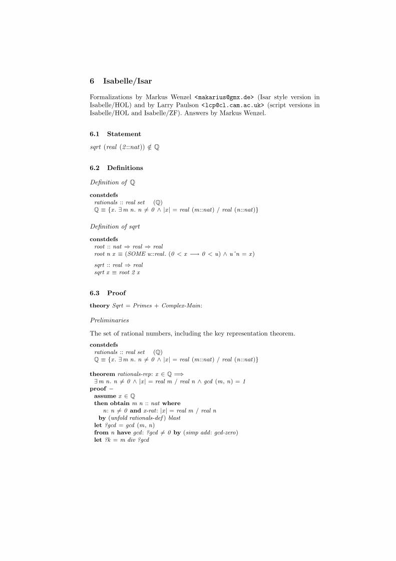
6 Isabelle/Isar
Formalizations by Markus Wenzel <[email protected]> (Isar style version inIsabelle/HOL) and by Larry Paulson <[email protected]> (script versions inIsabelle/HOL and Isabelle/ZF). Answers by Markus Wenzel.
6.1 Statement
sqrt (real (2 ::nat)) /∈ Q
6.2 Definitions
Definition of Q
constdefs
rationals :: real set (Q)Q ≡ x . ∃m n. n 6= 0 ∧ |x | = real (m::nat) / real (n::nat)
Definition of sqrt
constdefs
root :: nat ⇒ real ⇒ realroot n x ≡ (SOME u::real . (0 < x −→ 0 < u) ∧ uˆn = x )
sqrt :: real ⇒ realsqrt x ≡ root 2 x
6.3 Proof
theory Sqrt = Primes + Complex-Main:
Preliminaries
The set of rational numbers, including the key representation theorem.
constdefs
rationals :: real set (Q)Q ≡ x . ∃m n. n 6= 0 ∧ |x | = real (m::nat) / real (n::nat)
theorem rationals-rep: x ∈ Q =⇒∃m n. n 6= 0 ∧ |x | = real m / real n ∧ gcd (m, n) = 1
proof −assume x ∈ Q
then obtain m n :: nat where
n: n 6= 0 and x-rat : |x | = real m / real nby (unfold rationals-def ) blast
let ?gcd = gcd (m, n)from n have gcd : ?gcd 6= 0 by (simp add : gcd-zero)let ?k = m div ?gcd
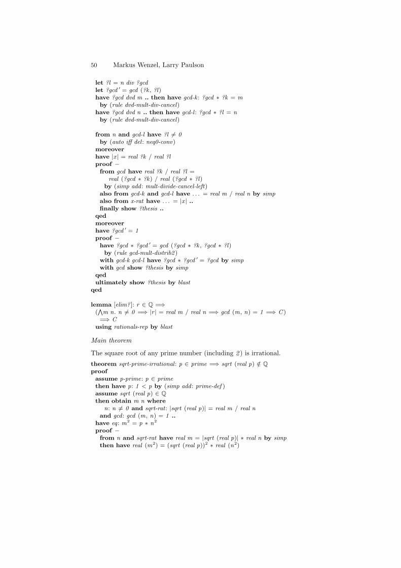
50 Markus Wenzel, Larry Paulson
let ?l = n div ?gcdlet ?gcd ′ = gcd (?k , ?l)have ?gcd dvd m .. then have gcd-k : ?gcd ∗ ?k = mby (rule dvd-mult-div-cancel)
have ?gcd dvd n .. then have gcd-l : ?gcd ∗ ?l = nby (rule dvd-mult-div-cancel)
from n and gcd-l have ?l 6= 0by (auto iff del : neq0-conv)
moreover
have |x | = real ?k / real ?lproof −from gcd have real ?k / real ?l =
real (?gcd ∗ ?k) / real (?gcd ∗ ?l)by (simp add : mult-divide-cancel-left)
also from gcd-k and gcd-l have . . . = real m / real n by simpalso from x-rat have . . . = |x | ..
finally show ?thesis ..
qed
moreover
have ?gcd ′ = 1proof −have ?gcd ∗ ?gcd ′ = gcd (?gcd ∗ ?k , ?gcd ∗ ?l)by (rule gcd-mult-distrib2 )
with gcd-k gcd-l have ?gcd ∗ ?gcd ′ = ?gcd by simpwith gcd show ?thesis by simp
qed
ultimately show ?thesis by blastqed
lemma [elim? ]: r ∈ Q =⇒(V
m n. n 6= 0 =⇒ |r | = real m / real n =⇒ gcd (m, n) = 1 =⇒ C )=⇒ C
using rationals-rep by blast
Main theorem
The square root of any prime number (including 2 ) is irrational.
theorem sqrt-prime-irrational : p ∈ prime =⇒ sqrt (real p) /∈ Q
proof
assume p-prime: p ∈ primethen have p: 1 < p by (simp add : prime-def )assume sqrt (real p) ∈ Q
then obtain m n where
n: n 6= 0 and sqrt-rat : |sqrt (real p)| = real m / real nand gcd : gcd (m, n) = 1 ..
have eq : m2 = p ∗ n2
proof −from n and sqrt-rat have real m = |sqrt (real p)| ∗ real n by simpthen have real (m2) = (sqrt (real p))2 ∗ real (n2)
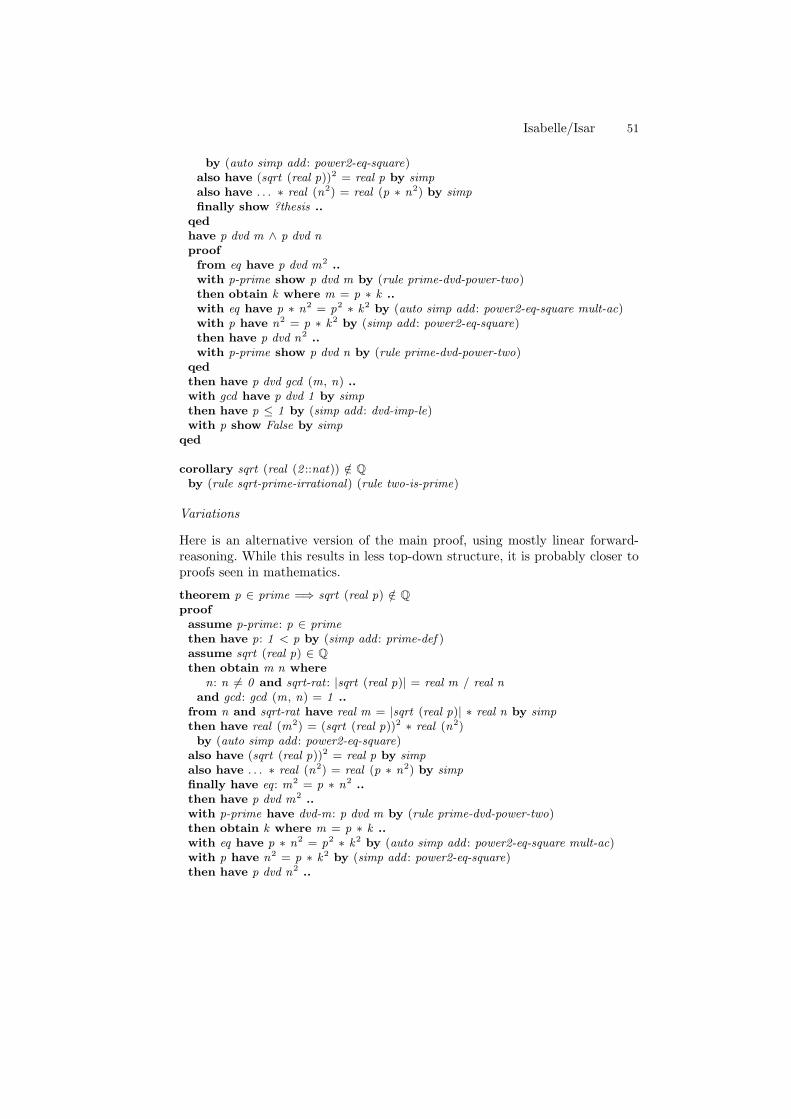
Isabelle/Isar 51
by (auto simp add : power2-eq-square)also have (sqrt (real p))2 = real p by simpalso have . . . ∗ real (n2) = real (p ∗ n2) by simpfinally show ?thesis ..
qed
have p dvd m ∧ p dvd nproof
from eq have p dvd m2 ..
with p-prime show p dvd m by (rule prime-dvd-power-two)then obtain k where m = p ∗ k ..
with eq have p ∗ n2 = p2 ∗ k2 by (auto simp add : power2-eq-square mult-ac)with p have n2 = p ∗ k2 by (simp add : power2-eq-square)then have p dvd n2 ..
with p-prime show p dvd n by (rule prime-dvd-power-two)qed
then have p dvd gcd (m, n) ..
with gcd have p dvd 1 by simpthen have p ≤ 1 by (simp add : dvd-imp-le)with p show False by simp
qed
corollary sqrt (real (2 ::nat)) /∈ Q
by (rule sqrt-prime-irrational) (rule two-is-prime)
Variations
Here is an alternative version of the main proof, using mostly linear forward-reasoning. While this results in less top-down structure, it is probably closer toproofs seen in mathematics.
theorem p ∈ prime =⇒ sqrt (real p) /∈ Q
proof
assume p-prime: p ∈ primethen have p: 1 < p by (simp add : prime-def )assume sqrt (real p) ∈ Q
then obtain m n where
n: n 6= 0 and sqrt-rat : |sqrt (real p)| = real m / real nand gcd : gcd (m, n) = 1 ..
from n and sqrt-rat have real m = |sqrt (real p)| ∗ real n by simpthen have real (m2) = (sqrt (real p))2 ∗ real (n2)by (auto simp add : power2-eq-square)
also have (sqrt (real p))2 = real p by simpalso have . . . ∗ real (n2) = real (p ∗ n2) by simpfinally have eq : m2 = p ∗ n2 ..
then have p dvd m2 ..
with p-prime have dvd-m: p dvd m by (rule prime-dvd-power-two)then obtain k where m = p ∗ k ..
with eq have p ∗ n2 = p2 ∗ k2 by (auto simp add : power2-eq-square mult-ac)with p have n2 = p ∗ k2 by (simp add : power2-eq-square)then have p dvd n2 ..
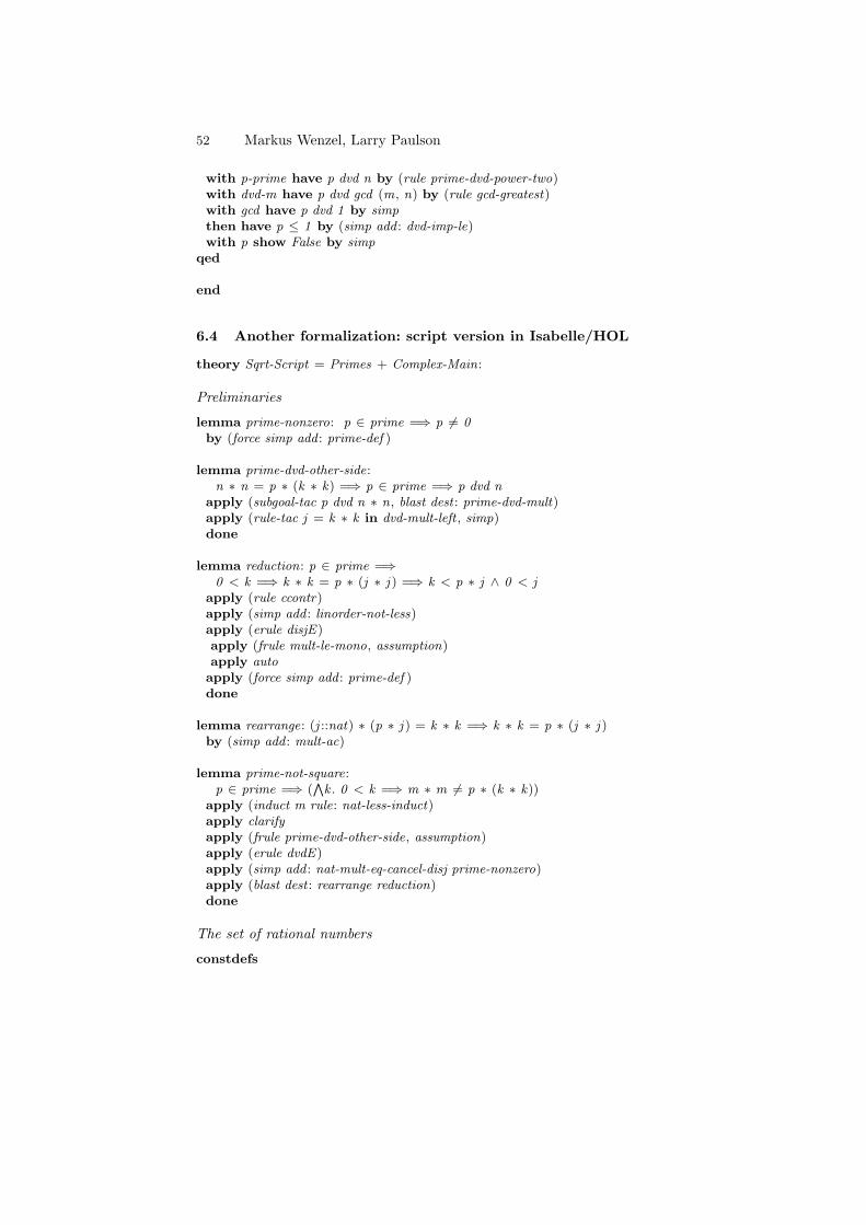
52 Markus Wenzel, Larry Paulson
with p-prime have p dvd n by (rule prime-dvd-power-two)with dvd-m have p dvd gcd (m, n) by (rule gcd-greatest)with gcd have p dvd 1 by simpthen have p ≤ 1 by (simp add : dvd-imp-le)with p show False by simp
qed
end
6.4 Another formalization: script version in Isabelle/HOL
theory Sqrt-Script = Primes + Complex-Main:
Preliminaries
lemma prime-nonzero: p ∈ prime =⇒ p 6= 0by (force simp add : prime-def )
lemma prime-dvd-other-side:n ∗ n = p ∗ (k ∗ k) =⇒ p ∈ prime =⇒ p dvd n
apply (subgoal-tac p dvd n ∗ n, blast dest : prime-dvd-mult)apply (rule-tac j = k ∗ k in dvd-mult-left , simp)done
lemma reduction: p ∈ prime =⇒0 < k =⇒ k ∗ k = p ∗ (j ∗ j ) =⇒ k < p ∗ j ∧ 0 < j
apply (rule ccontr)apply (simp add : linorder-not-less)apply (erule disjE)apply (frule mult-le-mono, assumption)apply autoapply (force simp add : prime-def )done
lemma rearrange: (j ::nat) ∗ (p ∗ j ) = k ∗ k =⇒ k ∗ k = p ∗ (j ∗ j )by (simp add : mult-ac)
lemma prime-not-square:p ∈ prime =⇒ (
Vk . 0 < k =⇒ m ∗ m 6= p ∗ (k ∗ k))
apply (induct m rule: nat-less-induct)apply clarifyapply (frule prime-dvd-other-side, assumption)apply (erule dvdE)apply (simp add : nat-mult-eq-cancel-disj prime-nonzero)apply (blast dest : rearrange reduction)done
The set of rational numbers
constdefs
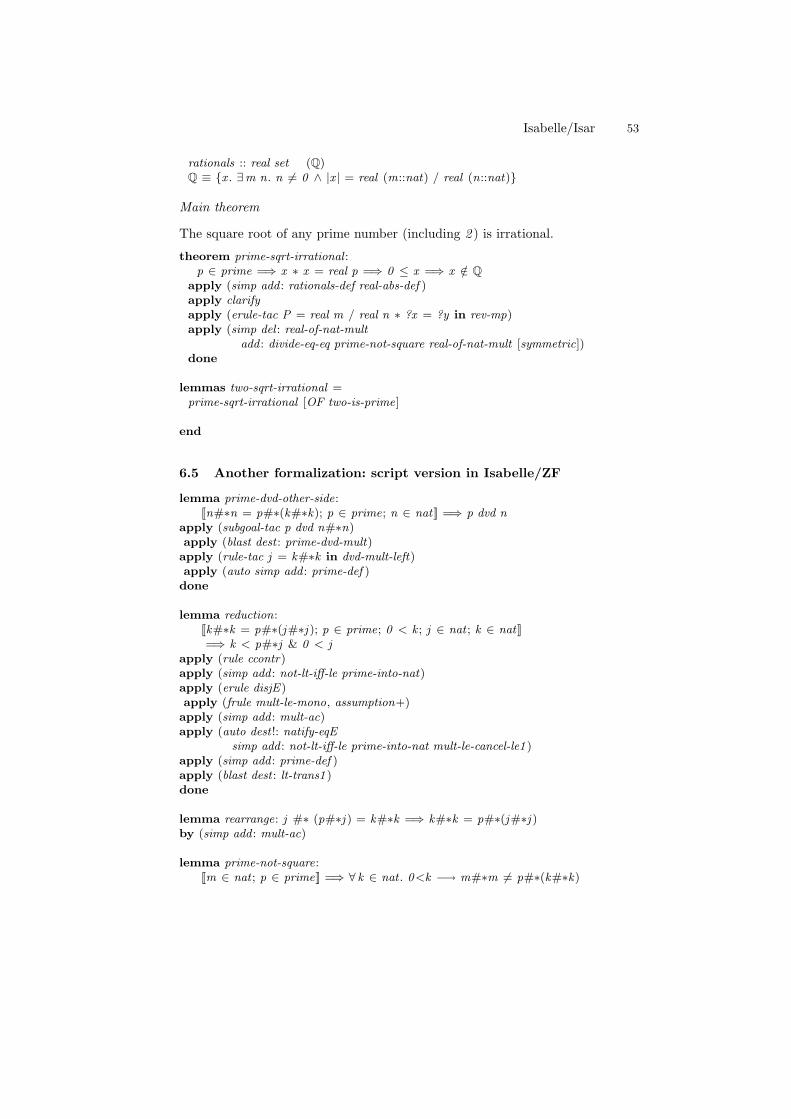
Isabelle/Isar 53
rationals :: real set (Q)Q ≡ x . ∃m n. n 6= 0 ∧ |x | = real (m::nat) / real (n::nat)
Main theorem
The square root of any prime number (including 2 ) is irrational.
theorem prime-sqrt-irrational :p ∈ prime =⇒ x ∗ x = real p =⇒ 0 ≤ x =⇒ x /∈ Q
apply (simp add : rationals-def real-abs-def )apply clarifyapply (erule-tac P = real m / real n ∗ ?x = ?y in rev-mp)apply (simp del : real-of-nat-mult
add : divide-eq-eq prime-not-square real-of-nat-mult [symmetric])done
lemmas two-sqrt-irrational =prime-sqrt-irrational [OF two-is-prime]
end
6.5 Another formalization: script version in Isabelle/ZF
lemma prime-dvd-other-side:[[n#∗n = p#∗(k#∗k); p ∈ prime; n ∈ nat ]] =⇒ p dvd n
apply (subgoal-tac p dvd n#∗n)apply (blast dest : prime-dvd-mult)apply (rule-tac j = k#∗k in dvd-mult-left)apply (auto simp add : prime-def )done
lemma reduction:[[k#∗k = p#∗(j#∗j ); p ∈ prime; 0 < k ; j ∈ nat ; k ∈ nat ]]=⇒ k < p#∗j & 0 < j
apply (rule ccontr)apply (simp add : not-lt-iff-le prime-into-nat)apply (erule disjE)apply (frule mult-le-mono, assumption+)apply (simp add : mult-ac)apply (auto dest !: natify-eqE
simp add : not-lt-iff-le prime-into-nat mult-le-cancel-le1 )apply (simp add : prime-def )apply (blast dest : lt-trans1 )done
lemma rearrange: j #∗ (p#∗j ) = k#∗k =⇒ k#∗k = p#∗(j#∗j )by (simp add : mult-ac)
lemma prime-not-square:[[m ∈ nat ; p ∈ prime]] =⇒ ∀ k ∈ nat . 0<k −→ m#∗m 6= p#∗(k#∗k)
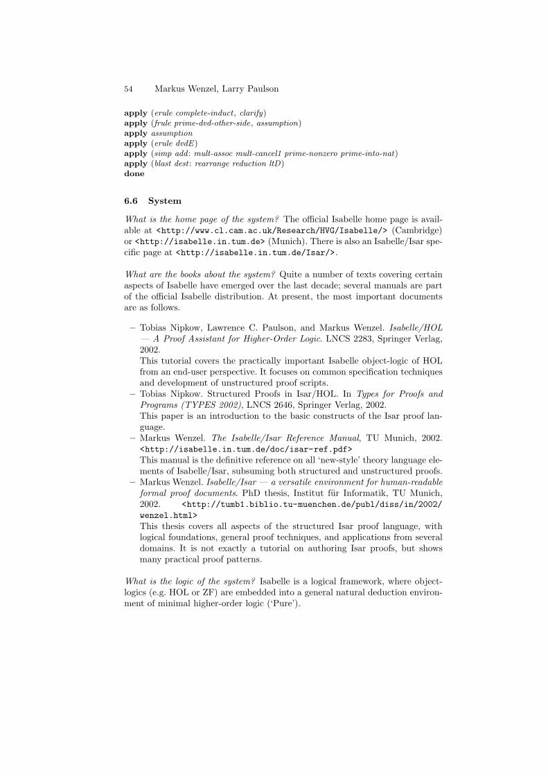
54 Markus Wenzel, Larry Paulson
apply (erule complete-induct , clarify)apply (frule prime-dvd-other-side, assumption)apply assumptionapply (erule dvdE)apply (simp add : mult-assoc mult-cancel1 prime-nonzero prime-into-nat)apply (blast dest : rearrange reduction ltD)done
6.6 System
What is the home page of the system? The official Isabelle home page is avail-able at <http://www.cl.cam.ac.uk/Research/HVG/Isabelle/> (Cambridge)or <http://isabelle.in.tum.de> (Munich). There is also an Isabelle/Isar spe-cific page at <http://isabelle.in.tum.de/Isar/>.
What are the books about the system? Quite a number of texts covering certainaspects of Isabelle have emerged over the last decade; several manuals are partof the official Isabelle distribution. At present, the most important documentsare as follows.
– Tobias Nipkow, Lawrence C. Paulson, and Markus Wenzel. Isabelle/HOL— A Proof Assistant for Higher-Order Logic. LNCS 2283, Springer Verlag,2002.This tutorial covers the practically important Isabelle object-logic of HOLfrom an end-user perspective. It focuses on common specification techniquesand development of unstructured proof scripts.
– Tobias Nipkow. Structured Proofs in Isar/HOL. In Types for Proofs andPrograms (TYPES 2002), LNCS 2646, Springer Verlag, 2002.This paper is an introduction to the basic constructs of the Isar proof lan-guage.
– Markus Wenzel. The Isabelle/Isar Reference Manual, TU Munich, 2002.<http://isabelle.in.tum.de/doc/isar-ref.pdf>
This manual is the definitive reference on all ‘new-style’ theory language ele-ments of Isabelle/Isar, subsuming both structured and unstructured proofs.
– Markus Wenzel. Isabelle/Isar — a versatile environment for human-readableformal proof documents. PhD thesis, Institut fur Informatik, TU Munich,2002. <http://tumb1.biblio.tu-muenchen.de/publ/diss/in/2002/
wenzel.html>
This thesis covers all aspects of the structured Isar proof language, withlogical foundations, general proof techniques, and applications from severaldomains. It is not exactly a tutorial on authoring Isar proofs, but showsmany practical proof patterns.
What is the logic of the system? Isabelle is a logical framework, where object-logics (e.g. HOL or ZF) are embedded into a general natural deduction environ-ment of minimal higher-order logic (‘Pure’).
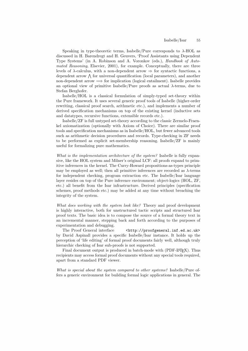
Isabelle/Isar 55
Speaking in type-theoretic terms, Isabelle/Pure corresponds to λ-HOL asdiscussed in H. Barendregt and H. Geuvers, ‘Proof Assistants using DependentType Systems’ (in A. Robinson and A. Voronkov (eds.), Handbook of Auto-mated Reasoning, Elsevier, 2001), for example. Conceptually, there are threelevels of λ-calculus, with a non-dependent arrow ⇒ for syntactic functions, adependent arrow
∧
for universal quantification (local parameters), and anothernon-dependent arrow =⇒ for implication (logical entailment). Isabelle providesan optional view of primitive Isabelle/Pure proofs as actual λ-terms, due toStefan Berghofer.
Isabelle/HOL is a classical formulation of simply-typed set-theory withinthe Pure framework. It uses several generic proof tools of Isabelle (higher-orderrewriting, classical proof search, arithmetic etc.), and implements a number ofderived specification mechanisms on top of the existing kernel (inductive setsand datatypes, recursive functions, extensible records etc.).
Isabelle/ZF is full untyped set-theory according to the classic Zermelo-Fraen-kel axiomatization (optionally with Axiom of Choice). There are similar prooftools and specification mechanisms as in Isabelle/HOL, but fewer advanced toolssuch as arithmetic decision procedures and records. Type-checking in ZF needsto be performed as explicit set-membership reasoning. Isabelle/ZF is mainlyuseful for formalizing pure mathematics.
What is the implementation architecture of the system? Isabelle is fully expan-sive, like the HOL system and Milner’s original LCF: all proofs expand to prim-itive inferences in the kernel. The Curry-Howard propositions-as-types principlemay be employed as well; then all primitive inferences are recorded as λ-termsfor independent checking, program extraction etc. The Isabelle/Isar languagelayer resides on top of the Pure inference environment; object-logics (HOL, ZF,etc.) all benefit from the Isar infrastructure. Derived principles (specificationschemes, proof methods etc.) may be added at any time without breaching theintegrity of the system.
What does working with the system look like? Theory and proof developmentis highly interactive, both for unstructured tactic scripts and structured Isarproof texts. The basic idea is to compose the source of a formal theory text inan incremental manner, stepping back and forth according to the purposes ofexperimentation and debugging.
The Proof General interface <http://proofgeneral.inf.ed.ac.uk>
by David Aspinall provides a specific Isabelle/Isar instance. It holds up theperception of ‘life editing’ of formal proof documents fairly well, although trulyhierarchic checking of Isar sub-proofs is not supported.
Final document output is produced in batch-mode with (PDF-LATEX). Thusrecipients may access formal proof documents without any special tools required,apart from a standard PDF viewer.
What is special about the system compared to other systems? Isabelle/Pure of-fers a generic environment for building formal logic applications in general. The
56 Markus Wenzel, Larry Paulson
Isabelle/Isar layer provides a rich infrastructure for high-level proof schemes,with a special focus on human-readable formal proof documents. Structuredand unstructured proofs may be freely intermixed within Isabelle/Isar theorydevelopments. The Isabelle distribution includes Isabelle/HOL as an end-userenvironment with many proven applications in mathematical modeling and ver-ification. There is also a document preparation system for turning the Isabelletheory sources into high-quality typeset output (as a side-effect of formal pro-cessing).
What are other versions of the system? There is essentially just one main trunkof Isabelle development, which evolves over time in a linear fashion (Isabelle2002,Isabelle2003, Isabelle2004 etc.).
Who are the people behind the system? The key players are Lawrence C. Paulson(Cambridge), Tobias Nipkow (Munich), and Markus Wenzel (Munich). StefanBerghofer (Munich) and Gerwin Klein (Munich and Sydney) have made substan-tial contributions. Many other people have participated in Isabelle development.
What are the main user communities of the system? Researchers and students ofcomputer-science and mathematics worldwide. A significant number of Isabelleusers are from outside of the original sites of Cambridge or Munich.
What large mathematical formalizations have been done in the system? A mas-sive body of Isabelle applications have emerged over the years. The largest oneis the Java formalization of the projects Bali <http://isabelle.in.tum.de/bali/> and VerifiCard <http://isabelle.in.tum.de/verificard/>, whichwere later combined into a unified whole <http://www.in.tum.de/~nipkow/
Jinja/> (as described by Gerwin Klein and Tobias Nipkow in ‘A Machine-Checked Model for a Java-Like Language, Virtual Machine and Compiler’, tobe published in TOPLAS ). Some properly ‘mathematical’ ones are part of thestandard library, such as <http://isabelle.in.tum.de/library/HOL/
HOL-Algebra/document.pdf> or <HOL-Complex/HahnBanach/document.pdf>.The largest of these is the formalization of Godel’s proof of the relative con-sistency of the axiom of choice, <http://isabelle.in.tum.de/library/ZF/Constructible/document.pdf>.
The Archive of Formal Proofs <http://afp.sourceforge.net/> is a collec-tion of proof libraries, examples, and larger scientific developments, mechanicallychecked in Isabelle. It is organized in the way of a scientific journal. Submissionsare refereed.
What representation of the formalization has been put in this paper? The for-malization follows common mathematical practice; both HOL and ZF providean adequate background theory for standard mathematics.
Isabelle/Isar 57
What needs to be explained about this specific proof? Isabelle/Isar proof textsare meant to be self-explanatory, at least well-written ones. The present examplehas been conducted realistically in the sense that any ‘omissions’ of the existingbackground library are included in full. The main proofs have been laid outto represent the logical structure of the argument adequately, without havingexcessive formal detail clutter the text. The general style of writing is up to theauthor; the Isar proof language is very flexible in that respect.
The Isabelle/HOL and Isabelle/ZF variants given in tactical style representthe typical manner of unstructured proof composition in Isabelle. The unstruc-tured Isabelle/HOL proof uses the same background library as the structuredIsar text.
The formalizations of the irrationality of√
2 from this section can be found inthe Isabelle2004 distribution as:
src/HOL/Complex/ex/Sqrt.thy
src/HOL/Complex/ex/Sqrt_Script.thy
src/ZF/ex/Primes.thy
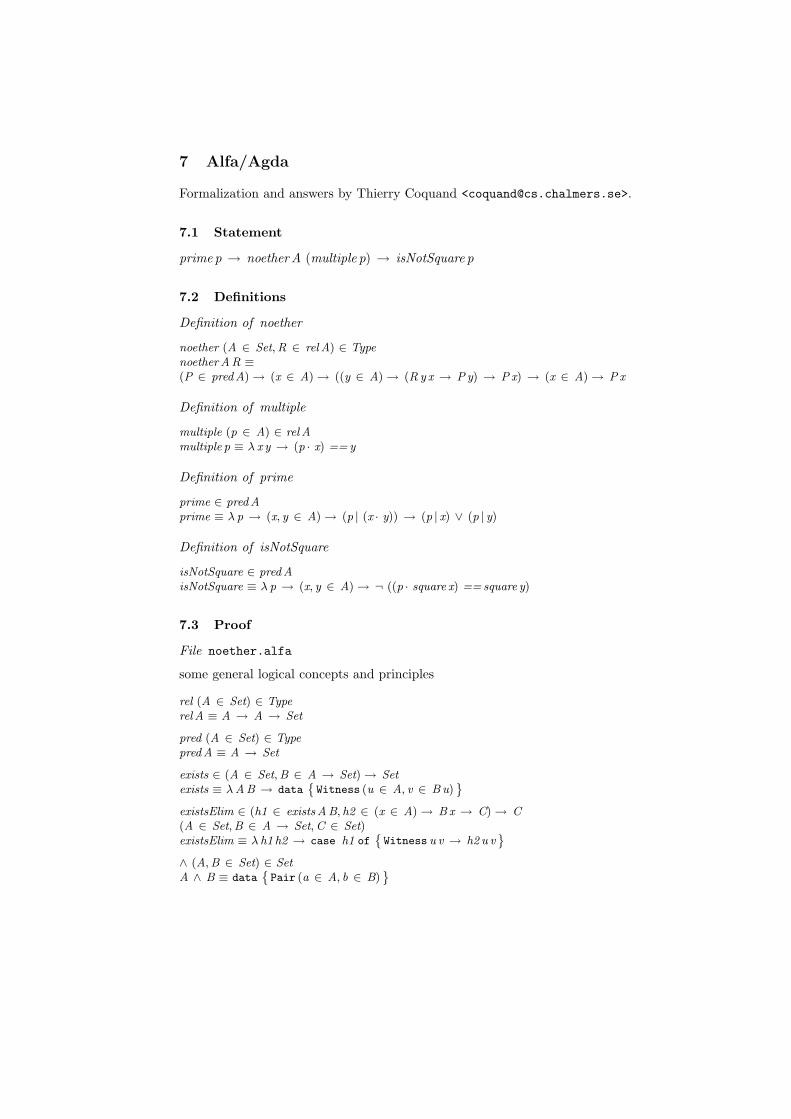
7 Alfa/Agda
Formalization and answers by Thierry Coquand <[email protected]>.
7.1 Statement
prime p → noetherA (multiple p) → isNotSquare p
7.2 Definitions
Definition of noether
noether (A ∈ Set,R ∈ rel A) ∈ TypenoetherAR ≡(P ∈ predA) → (x ∈ A) → ((y ∈ A) → (Ry x → Py) → Px) → (x ∈ A) → Px
Definition of multiple
multiple (p ∈ A) ∈ rel Amultiple p ≡ λ x y → (p · x) ==y
Definition of prime
prime ∈ predAprime ≡ λ p → (x, y ∈ A) → (p | (x · y)) → (p | x) ∨ (p | y)
Definition of isNotSquare
isNotSquare ∈ predAisNotSquare ≡ λ p → (x, y ∈ A) → ¬ ((p · square x) ==square y)
7.3 Proof
File noether.alfa
some general logical concepts and principles
rel (A ∈ Set) ∈ Typerel A ≡ A → A → Set
pred (A ∈ Set) ∈ TypepredA ≡ A → Set
exists ∈ (A ∈ Set,B ∈ A → Set) → Setexists ≡ λAB → data
˘Witness (u ∈ A, v ∈ Bu)
¯
existsElim ∈ (h1 ∈ existsAB, h2 ∈ (x ∈ A) → Bx → C) → C(A ∈ Set,B ∈ A → Set,C ∈ Set)existsElim ≡ λ h1 h2 → case h1 of
˘Witness u v → h2 u v
¯
∧ (A,B ∈ Set) ∈ SetA ∧ B ≡ data
˘Pair (a ∈ A, b ∈ B)
¯
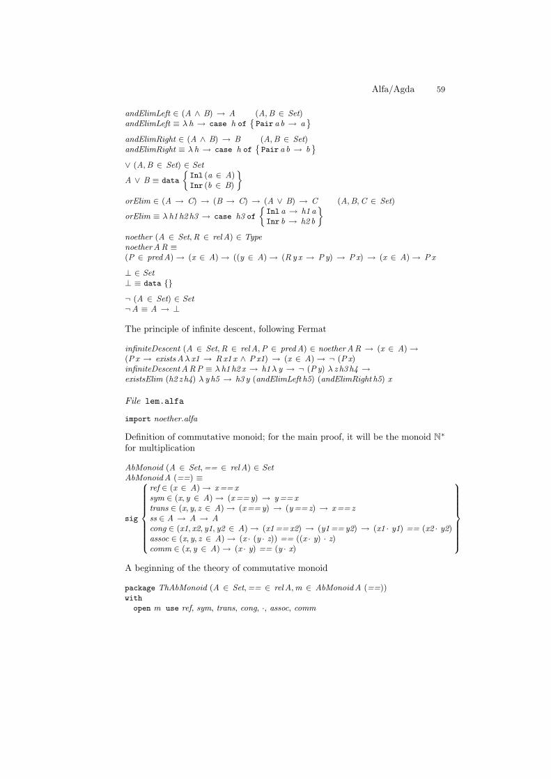
Alfa/Agda 59
andElimLeft ∈ (A ∧ B) → A (A,B ∈ Set)andElimLeft ≡ λ h → case h of
˘Pair a b → a
¯
andElimRight ∈ (A ∧ B) → B (A,B ∈ Set)andElimRight ≡ λ h → case h of
˘Pair a b → b
¯
∨ (A,B ∈ Set) ∈ Set
A ∨ B ≡ data
Inl (a ∈ A)Inr (b ∈ B)
ff
orElim ∈ (A → C) → (B → C) → (A ∨ B) → C (A,B,C ∈ Set)
orElim ≡ λ h1 h2 h3 → case h3 of
Inl a → h1 aInr b → h2 b
ff
noether (A ∈ Set,R ∈ rel A) ∈ TypenoetherAR ≡(P ∈ predA) → (x ∈ A) → ((y ∈ A) → (Ry x → Py) → Px) → (x ∈ A) → Px
⊥ ∈ Set⊥ ≡ data
¬ (A ∈ Set) ∈ Set¬A ≡ A → ⊥
The principle of infinite descent, following Fermat
infiniteDescent (A ∈ Set,R ∈ rel A,P ∈ predA) ∈ noetherAR → (x ∈ A) →(Px → existsAλ x1 → Rx1 x ∧ Px1) → (x ∈ A) → ¬ (Px)infiniteDescentARP ≡ λ h1 h2 x → h1λ y → ¬ (Py) λ z h3 h4 →existsElim (h2 z h4) λ y h5 → h3 y (andElimLeft h5) (andElimRight h5) x
File lem.alfa
import noether.alfa
Definition of commutative monoid; for the main proof, it will be the monoid N∗
for multiplication
AbMonoid (A ∈ Set,== ∈ rel A) ∈ SetAbMonoidA (==) ≡
sig
8>>>>>>>><>>>>>>>>:
ref ∈ (x ∈ A) → x==xsym ∈ (x, y ∈ A) → (x==y) → y==xtrans ∈ (x, y, z ∈ A) → (x==y) → (y== z) → x== zss ∈ A → A → Acong ∈ (x1, x2, y1, y2 ∈ A) → (x1==x2) → (y1==y2) → (x1 · y1) == (x2 · y2)assoc ∈ (x, y, z ∈ A) → (x · (y · z)) == ((x · y) · z)comm ∈ (x, y ∈ A) → (x · y) == (y · x)
9>>>>>>>>=>>>>>>>>;
A beginning of the theory of commutative monoid
package ThAbMonoid (A ∈ Set,== ∈ rel A,m ∈ AbMonoidA (==))with
open m use ref, sym, trans, cong, ·, assoc, comm
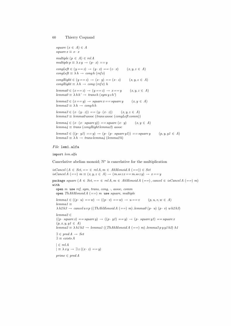
60 Thierry Coquand
square (x ∈ A) ∈ Asquare x ≡ x · x
multiple (p ∈ A) ∈ rel Amultiple p ≡ λ x y → (p · x) ==y
congLeft ∈ (y== z) → (y · x) == (z · x) (x, y, z ∈ A)congLeft ≡ λ h → cong h (ref x)
congRight ∈ (y== z) → (x · y) == (x · z) (x, y, z ∈ A)congRight ≡ λ h → cong (ref x) h
lemma0 ∈ (x== z) → (y== z) → x==y (x, y, z ∈ A)lemma0 ≡ λ h h’ → trans h (symy z h’)
lemma2 ∈ (x==y) → square x== square y (x, y ∈ A)lemma2 ≡ λ h → cong h h
lemma3 ∈ (x · (y · z)) == (y · (x · z)) (x, y, z ∈ A)lemma3 ≡ lemma0 assoc (trans assoc (congLeft comm))
lemma4 ∈ (x · (x · square y)) ==square (x · y) (x, y ∈ A)lemma4 ≡ trans (congRight lemma3) assoc
lemma5 ∈ ((p · y1) ==y) → (p · (p · square y1)) ==square y (p, y, y1 ∈ A)lemma5 ≡ λ h → trans lemma4 (lemma2 h)
File lem1.alfa
import lem.alfa
Cancelative abelian monoid; N∗ is cancelative for the multiplication
isCancel (A ∈ Set,== ∈ rel A,m ∈ AbMonoidA (==)) ∈ SetisCancel A (==) m ≡ (x, y, z ∈ A) → (m.ss z x==m.ss z y) → x==y
package square (A ∈ Set,== ∈ rel A,m ∈ AbMonoidA (==) , cancel ∈ isCancel A (==) m)with
open m use ref, sym, trans, cong, ·, assoc, commopen ThAbMonoidA (==) m use square, multiple
lemma1 ∈ ((p · u) ==w) → ((p · v) ==w) → u==v (p, u, v,w ∈ A)lemma1 ≡λ h2 h3 → cancel u v p ((ThAbMonoidA (==) m) .lemma0 (p · u) (p · v) wh2 h3)
lemma2 ∈((p · square x) ==square y) → ((p · y1) ==y) → (p · square y1) ==square x(p, x, y, y1 ∈ A)lemma2 ≡ λ h1 h2 → lemma1 ((ThAbMonoidA (==) m) .lemma5 p y y1 h2) h1
∃ ∈ predA → Set∃ ≡ existsA
| ∈ rel A| ≡ λ x y → ∃ z ((x · z) ==y)
prime ∈ predA
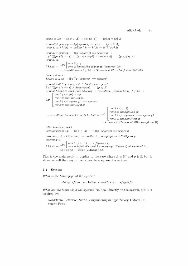
Alfa/Agda 61
prime ≡ λ p → (x, y ∈ A) → (p | (x · y)) → (p | x) ∨ (p | y)
lemma3 ∈ prime p → (p | square x) → p | x (p, x ∈ A)lemma3 ≡ λ h1 h2 → orElimλ h → hλ h → h (h1 x x h2)
lemma4 ∈ prime p → ((p · square x) ==square y) →∃ y1 (((p · y1) ==y) ∧ ((p · square y1) ==square x)) (p, x, y ∈ A)lemma4 ≡
λ h1 h2 → let
»rem ∈ p | yrem ≡ lemma3 h1 (Witness (square x) h2)
in existsElim remλ y1 h3 → Witness y1 (Pair h3 (lemma2 h2 h3))
Square ∈ rel ASquare ≡ λ p x → ∃ y ((p · square x) ==square y)
lemma5 (h2 ∈ prime p, x ∈ A, h3 ∈ Square p x) ∈∃ x1 (((p · x1) ==x) ∧ Square p x1) (p ∈ A)lemma5 h2 x h3 ≡ existsElim h3λ y h4 → existsElim (lemma4 h2 h4) λ y1 h5 →
let
2664
rem1 ∈ (p · y1) ==yrem1 ≡ andElimLeft h5rem2 ∈ (p · square y1) ==square xrem2 ≡ andElimRight h5
in existsElim (lemma4 h2 rem2) λ x1 h6 → let
2664
rem3 ∈ (p · x1) ==xrem3 ≡ andElimLeft h6rem4 ∈ (p · square x1) ==square y1rem4 ≡ andElimRight h6
in Witness x1 (Pair rem3 (Witness y1 rem4))
isNotSquare ∈ predAisNotSquare ≡ λ p → (x, y ∈ A) → ¬ ((p · square x) ==square y)
theorem (p ∈ A) ∈ prime p → noetherA (multiple p) → isNotSquare ptheoremp ≡
λ h1 h2 → let
»rem ∈ (x ∈ A) → ¬ (Square p x)rem ≡ infiniteDescentA (multiple p) (Square p) h2 (lemma5 h1)
inλ x y h3 → rem x (Witness y h3)
This is the main result; it applies to the case where A is N∗ and p is 2, but itshows as well that any prime cannot be a square of a rational
7.4 System
What is the home page of the system?
<http://www.cs.chalmers.se/~catarina/agda/>
What are the books about the system? No book directly on the system, but it isinspired by:
Nordstrom, Petersson, Smith, Programming in Type Theory, Oxford Uni-versity Press.
62 Thierry Coquand
What is the logic of the system? Described in Per Martin-Lof, ‘An intuitionistictheory of types’, 1972. It can be found in:
G. Sambin and J. Smith (eds.), 25 years of constructive type theory,Oxford University Press.
This is extended by general data type declaration and case notation.
What is the implementation architecture of the system? Described in <http:
//www.cs.chalmers.se/~catarina/agda/>.
What does working with the system look like? It feels like programming in a func-tional language with dependent types. The construction of the proof/programcan be done interactively with place-holders/meta-variables. Actually the syntaxis very close to the functional language Cayenne, designed by Lennart Augusts-son, <http://www.cs.chalmers.se/~augustss/cayenne/>.
What is special about the system compared to other systems? Identification ofproofs and functional programs with dependent types + meta-variables.
What are other versions of the system? A first version (1990) was written byThierry Coquand (caml) and Lennart Augustsson (C). Then (1992) version LenaMagnusson (SML) and Johan Nordlander (C).
Alfa is the interface of the system. It has been written by Thomas Hall-gren. There is also an Emacs interface, following ideas of Dan Synek, written byCatarina Coquand,
Who are the people behind the system? The meta-variable idea comes from BengtNordstrom, refined later by Thierry Coquand and Lena Magnusson. The previousversion Half was designed by Thierry Coquand (gofer) and Dan Synek (C). Theactual version is designed by Catarina Coquand (haskell).
What are the main user communities of the system? Peter Hancock and AntonSetzer.
What large mathematical formalizations have been done in the system? Localicversion of Hahn-Banach was done by Jan Cederquist in Half.
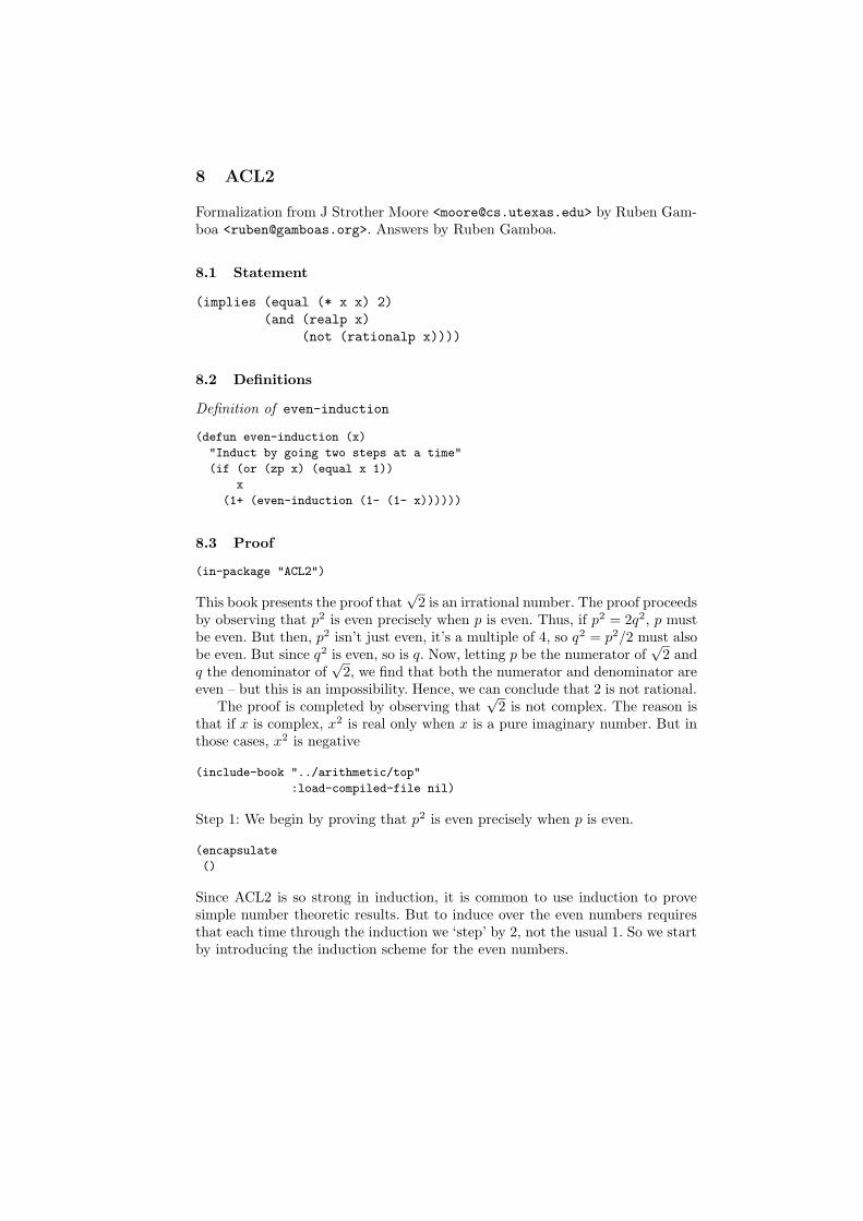
8 ACL2
Formalization from J Strother Moore <[email protected]> by Ruben Gam-boa <[email protected]>. Answers by Ruben Gamboa.
8.1 Statement
(implies (equal (* x x) 2)
(and (realp x)
(not (rationalp x))))
8.2 Definitions
Definition of even-induction
(defun even-induction (x)
"Induct by going two steps at a time"
(if (or (zp x) (equal x 1))
x
(1+ (even-induction (1- (1- x))))))
8.3 Proof
(in-package "ACL2")
This book presents the proof that√
2 is an irrational number. The proof proceedsby observing that p2 is even precisely when p is even. Thus, if p2 = 2q2, p mustbe even. But then, p2 isn’t just even, it’s a multiple of 4, so q2 = p2/2 must alsobe even. But since q2 is even, so is q. Now, letting p be the numerator of
√2 and
q the denominator of√
2, we find that both the numerator and denominator areeven – but this is an impossibility. Hence, we can conclude that 2 is not rational.
The proof is completed by observing that√
2 is not complex. The reason isthat if x is complex, x2 is real only when x is a pure imaginary number. But inthose cases, x2 is negative
(include-book "../arithmetic/top"
:load-compiled-file nil)
Step 1: We begin by proving that p2 is even precisely when p is even.
(encapsulate
()
Since ACL2 is so strong in induction, it is common to use induction to provesimple number theoretic results. But to induce over the even numbers requiresthat each time through the induction we ‘step’ by 2, not the usual 1. So we startby introducing the induction scheme for the even numbers.
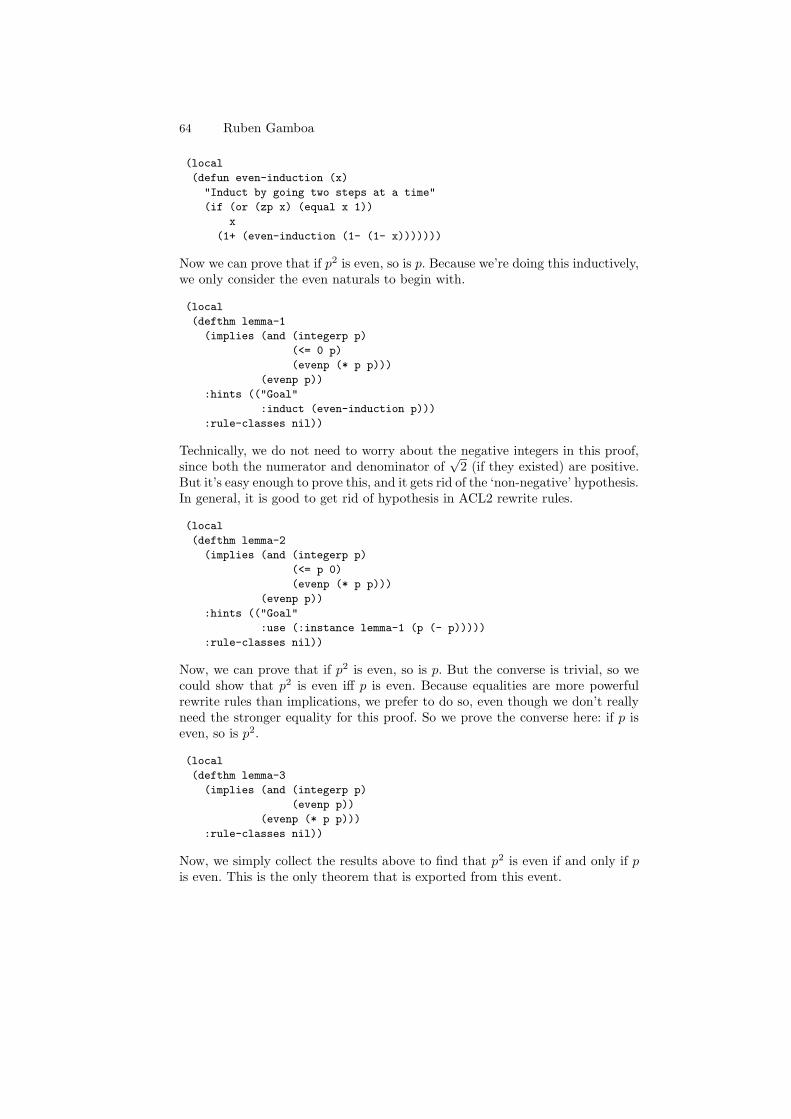
64 Ruben Gamboa
(local
(defun even-induction (x)
"Induct by going two steps at a time"
(if (or (zp x) (equal x 1))
x
(1+ (even-induction (1- (1- x)))))))
Now we can prove that if p2 is even, so is p. Because we’re doing this inductively,we only consider the even naturals to begin with.
(local
(defthm lemma-1
(implies (and (integerp p)
(<= 0 p)
(evenp (* p p)))
(evenp p))
:hints (("Goal"
:induct (even-induction p)))
:rule-classes nil))
Technically, we do not need to worry about the negative integers in this proof,since both the numerator and denominator of
√2 (if they existed) are positive.
But it’s easy enough to prove this, and it gets rid of the ‘non-negative’ hypothesis.In general, it is good to get rid of hypothesis in ACL2 rewrite rules.
(local
(defthm lemma-2
(implies (and (integerp p)
(<= p 0)
(evenp (* p p)))
(evenp p))
:hints (("Goal"
:use (:instance lemma-1 (p (- p)))))
:rule-classes nil))
Now, we can prove that if p2 is even, so is p. But the converse is trivial, so wecould show that p2 is even iff p is even. Because equalities are more powerfulrewrite rules than implications, we prefer to do so, even though we don’t reallyneed the stronger equality for this proof. So we prove the converse here: if p iseven, so is p2.
(local
(defthm lemma-3
(implies (and (integerp p)
(evenp p))
(evenp (* p p)))
:rule-classes nil))
Now, we simply collect the results above to find that p2 is even if and only if pis even. This is the only theorem that is exported from this event.
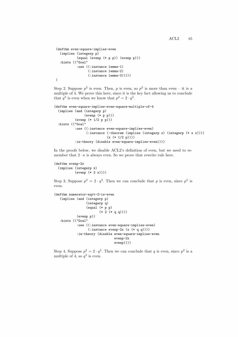
ACL2 65
(defthm even-square-implies-even
(implies (integerp p)
(equal (evenp (* p p)) (evenp p)))
:hints (("Goal"
:use ((:instance lemma-1)
(:instance lemma-2)
(:instance lemma-3)))))
)
Step 2. Suppose p2 is even. Then, p is even, so p2 is more than even – it is amultiple of 4. We prove this here, since it is the key fact allowing us to concludethat q2 is even when we know that p2 = 2 · q2.
(defthm even-square-implies-even-square-multiple-of-4
(implies (and (integerp p)
(evenp (* p p)))
(evenp (* 1/2 p p)))
:hints (("Goal"
:use ((:instance even-square-implies-even)
(:instance (:theorem (implies (integerp x) (integerp (* x x))))
(x (* 1/2 p))))
:in-theory (disable even-square-implies-even))))
In the proofs below, we disable ACL2’s definition of even, but we need to re-member that 2 · n is always even. So we prove that rewrite rule here.
(defthm evenp-2x
(implies (integerp x)
(evenp (* 2 x))))
Step 3. Suppose p2 = 2 · q2. Then we can conclude that p is even, since p2 iseven.
(defthm numerator-sqrt-2-is-even
(implies (and (integerp p)
(integerp q)
(equal (* p p)
(* 2 (* q q))))
(evenp p))
:hints (("Goal"
:use ((:instance even-square-implies-even)
(:instance evenp-2x (x (* q q))))
:in-theory (disable even-square-implies-even
evenp-2x
evenp))))
Step 4. Suppose p2 = 2 · q2. Then we can conclude that q is even, since p2 is amultiple of 4, so q2 is even.
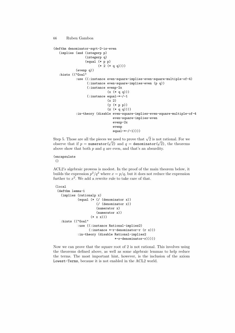
66 Ruben Gamboa
(defthm denominator-sqrt-2-is-even
(implies (and (integerp p)
(integerp q)
(equal (* p p)
(* 2 (* q q))))
(evenp q))
:hints (("Goal"
:use ((:instance even-square-implies-even-square-multiple-of-4)
(:instance even-square-implies-even (p q))
(:instance evenp-2x
(x (* q q)))
(:instance equal-*-/-1
(x 2)
(y (* p p))
(z (* q q))))
:in-theory (disable even-square-implies-even-square-multiple-of-4
even-square-implies-even
evenp-2x
evenp
equal-*-/-1))))
Step 5. Those are all the pieces we need to prove that√
2 is not rational. For weobserve that if p = numerator(
√2) and q = denominator(
√2), the theorems
above show that both p and q are even, and that’s an absurdity.
(encapsulate
()
ACL2’s algebraic prowess is modest. In the proof of the main theorem below, itbuilds the expression p2/q2 where x = p/q, but it does not reduce the expressionfurther to x2. We add a rewrite rule to take care of that.
(local
(defthm lemma-1
(implies (rationalp x)
(equal (* (/ (denominator x))
(/ (denominator x))
(numerator x)
(numerator x))
(* x x)))
:hints (("Goal"
:use ((:instance Rational-implies2)
(:instance *-r-denominator-r (r x)))
:in-theory (disable Rational-implies2
*-r-denominator-r)))))
Now we can prove that the square root of 2 is not rational. This involves usingthe theorems defined above, as well as some algebraic lemmas to help reducethe terms. The most important hint, however, is the inclusion of the axiomLowest-Terms, because it is not enabled in the ACL2 world.
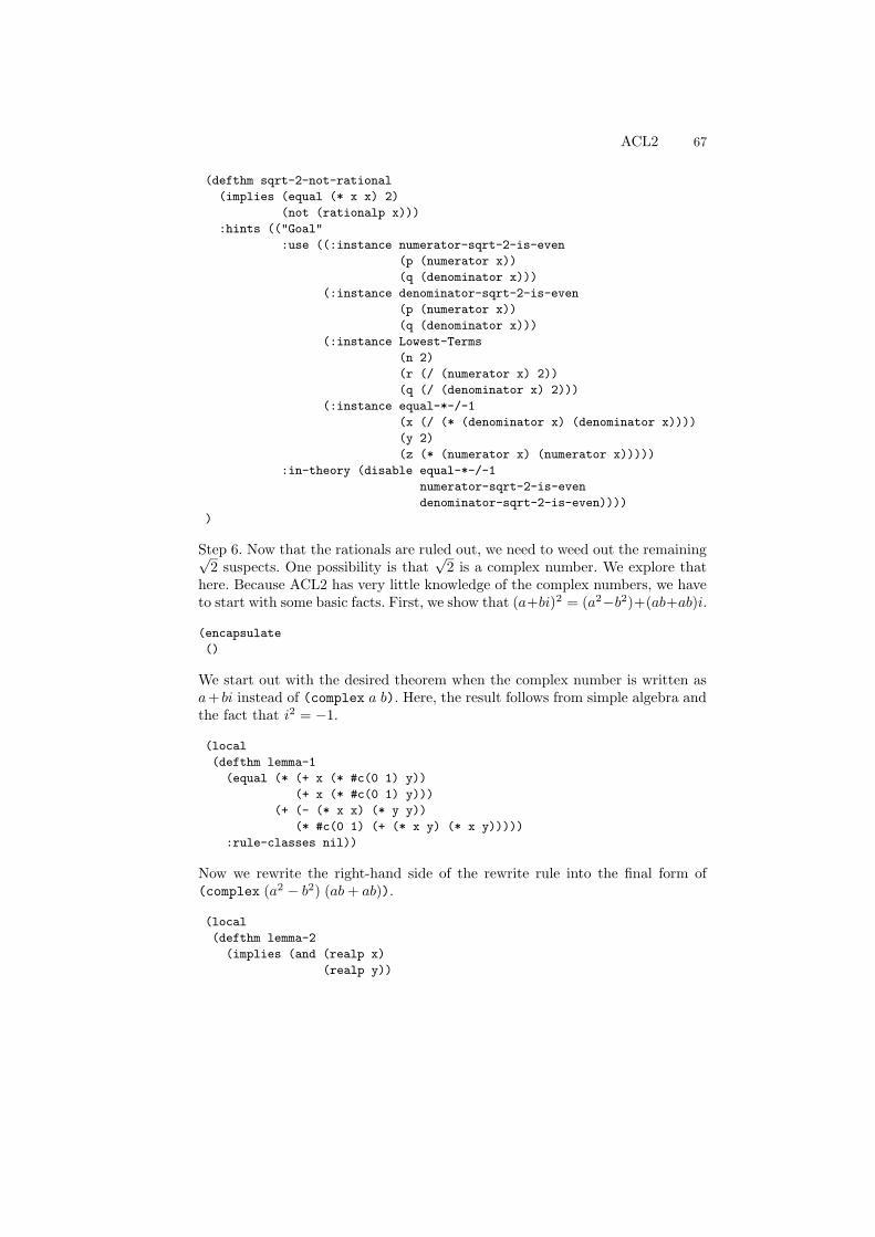
ACL2 67
(defthm sqrt-2-not-rational
(implies (equal (* x x) 2)
(not (rationalp x)))
:hints (("Goal"
:use ((:instance numerator-sqrt-2-is-even
(p (numerator x))
(q (denominator x)))
(:instance denominator-sqrt-2-is-even
(p (numerator x))
(q (denominator x)))
(:instance Lowest-Terms
(n 2)
(r (/ (numerator x) 2))
(q (/ (denominator x) 2)))
(:instance equal-*-/-1
(x (/ (* (denominator x) (denominator x))))
(y 2)
(z (* (numerator x) (numerator x)))))
:in-theory (disable equal-*-/-1
numerator-sqrt-2-is-even
denominator-sqrt-2-is-even))))
)
Step 6. Now that the rationals are ruled out, we need to weed out the remaining√2 suspects. One possibility is that
√2 is a complex number. We explore that
here. Because ACL2 has very little knowledge of the complex numbers, we haveto start with some basic facts. First, we show that (a+bi)2 = (a2−b2)+(ab+ab)i.
(encapsulate
()
We start out with the desired theorem when the complex number is written asa+ bi instead of (complex a b). Here, the result follows from simple algebra andthe fact that i2 = −1.
(local
(defthm lemma-1
(equal (* (+ x (* #c(0 1) y))
(+ x (* #c(0 1) y)))
(+ (- (* x x) (* y y))
(* #c(0 1) (+ (* x y) (* x y)))))
:rule-classes nil))
Now we rewrite the right-hand side of the rewrite rule into the final form of(complex (a2 − b2) (ab + ab)).
(local
(defthm lemma-2
(implies (and (realp x)
(realp y))
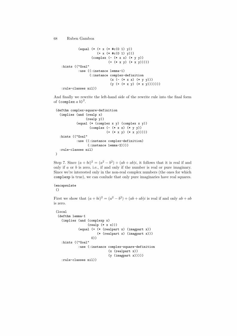
68 Ruben Gamboa
(equal (* (+ x (* #c(0 1) y))
(+ x (* #c(0 1) y)))
(complex (- (* x x) (* y y))
(+ (* x y) (* x y)))))
:hints (("Goal"
:use ((:instance lemma-1)
(:instance complex-definition
(x (- (* x x) (* y y)))
(y (+ (* x y) (* x y)))))))
:rule-classes nil))
And finally we rewrite the left-hand side of the rewrite rule into the final formof (complex a b)2.
(defthm complex-square-definition
(implies (and (realp x)
(realp y))
(equal (* (complex x y) (complex x y))
(complex (- (* x x) (* y y))
(+ (* x y) (* x y)))))
:hints (("Goal"
:use ((:instance complex-definition)
(:instance lemma-2))))
:rule-classes nil)
)
Step 7. Since (a + bi)2 = (a2 − b2) + (ab + ab)i, it follows that it is real if andonly if a or b is zero, i.e., if and only if the number is real or pure imaginary.Since we’re interested only in the non-real complex numbers (the ones for whichcomplexp is true), we can conlude that only pure imaginaries have real squares.
(encapsulate
()
First we show that (a + bi)2 = (a2 − b2) + (ab + ab)i is real if and only ab + abis zero.
(local
(defthm lemma-1
(implies (and (complexp x)
(realp (* x x)))
(equal (+ (* (realpart x) (imagpart x))
(* (realpart x) (imagpart x)))
0))
:hints (("Goal"
:use (:instance complex-square-definition
(x (realpart x))
(y (imagpart x)))))
:rule-classes nil))
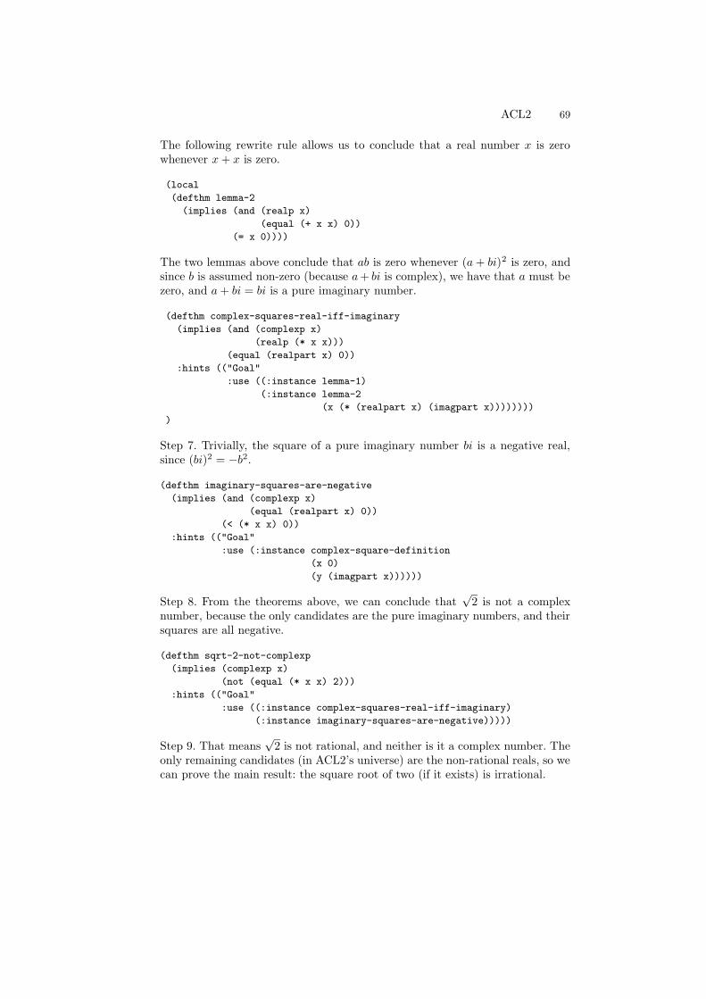
ACL2 69
The following rewrite rule allows us to conclude that a real number x is zerowhenever x + x is zero.
(local
(defthm lemma-2
(implies (and (realp x)
(equal (+ x x) 0))
(= x 0))))
The two lemmas above conclude that ab is zero whenever (a + bi)2 is zero, andsince b is assumed non-zero (because a + bi is complex), we have that a must bezero, and a + bi = bi is a pure imaginary number.
(defthm complex-squares-real-iff-imaginary
(implies (and (complexp x)
(realp (* x x)))
(equal (realpart x) 0))
:hints (("Goal"
:use ((:instance lemma-1)
(:instance lemma-2
(x (* (realpart x) (imagpart x))))))))
)
Step 7. Trivially, the square of a pure imaginary number bi is a negative real,since (bi)2 = −b2.
(defthm imaginary-squares-are-negative
(implies (and (complexp x)
(equal (realpart x) 0))
(< (* x x) 0))
:hints (("Goal"
:use (:instance complex-square-definition
(x 0)
(y (imagpart x))))))
Step 8. From the theorems above, we can conclude that√
2 is not a complexnumber, because the only candidates are the pure imaginary numbers, and theirsquares are all negative.
(defthm sqrt-2-not-complexp
(implies (complexp x)
(not (equal (* x x) 2)))
:hints (("Goal"
:use ((:instance complex-squares-real-iff-imaginary)
(:instance imaginary-squares-are-negative)))))
Step 9. That means√
2 is not rational, and neither is it a complex number. Theonly remaining candidates (in ACL2’s universe) are the non-rational reals, so wecan prove the main result: the square root of two (if it exists) is irrational.

70 Ruben Gamboa
(defthm irrational-sqrt-2
(implies (equal (* x x) 2)
(and (realp x)
(not (rationalp x))))
:hints (("Goal"
:cases ((rationalp x) (complexp x)))))
Step 10. Next, it would be nice to show that√
2 actually exists! See the booknonstd/nsa/sqrt.lisp for a proof of that, using non-standard analysis.
Output of lemma-1 of even-square-implies-even
ACL2(r) !>>>(LOCAL (DEFTHM LEMMA-1
(IMPLIES (AND (INTEGERP P)
(<= 0 P)
(EVENP (* P P)))
(EVENP P))
:HINTS
(("Goal" :INDUCT (EVEN-INDUCTION P)))
:RULE-CLASSES NIL))
[Note: A hint was supplied for our processing of the goal above.
Thanks!]
Name the formula above *1.
We have been told to use induction. One induction scheme is suggested
by the induction hint.
We will induct according to a scheme suggested by (EVEN-INDUCTION P).
If we let (:P P) denote *1 above then the induction scheme we’ll use
is
(AND (IMPLIES (AND (NOT (OR (ZP P) (EQUAL P 1)))
(:P (+ -1 -1 P)))
(:P P))
(IMPLIES (OR (ZP P) (EQUAL P 1))
(:P P))).
This induction is justified by the same argument used to admit EVEN-
INDUCTION, namely, the measure (ACL2-COUNT P) is decreasing according
to the relation E0-ORD-< (which is known to be well-founded on the
domain recognized by E0-ORDINALP). When applied to the goal at hand
the above induction scheme produces the following two nontautological
subgoals.
Subgoal *1/2
(IMPLIES (AND (NOT (OR (ZP P) (EQUAL P 1)))
(IMPLIES (AND (INTEGERP (+ -1 -1 P))
(<= 0 (+ -1 -1 P))
(EVENP (* (+ -1 -1 P) (+ -1 -1 P))))
(EVENP (+ -1 -1 P))))
(IMPLIES (AND (INTEGERP P)
(<= 0 P)
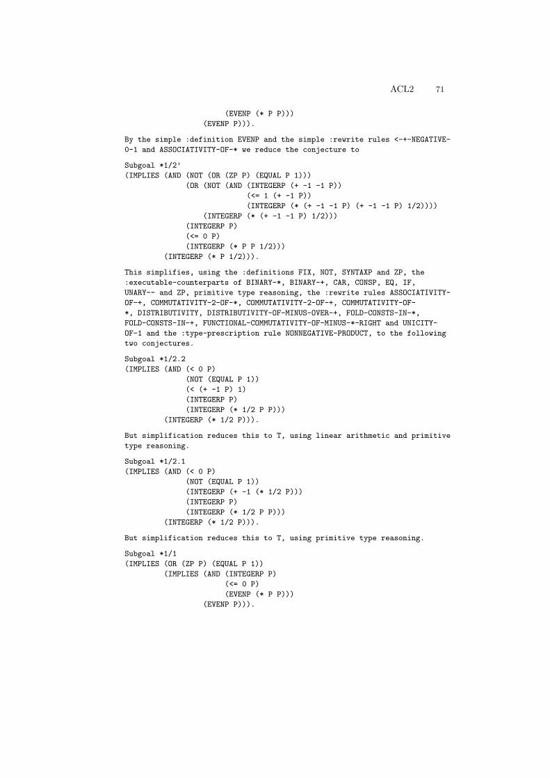
ACL2 71
(EVENP (* P P)))
(EVENP P))).
By the simple :definition EVENP and the simple :rewrite rules <-+-NEGATIVE-
0-1 and ASSOCIATIVITY-OF-* we reduce the conjecture to
Subgoal *1/2’
(IMPLIES (AND (NOT (OR (ZP P) (EQUAL P 1)))
(OR (NOT (AND (INTEGERP (+ -1 -1 P))
(<= 1 (+ -1 P))
(INTEGERP (* (+ -1 -1 P) (+ -1 -1 P) 1/2))))
(INTEGERP (* (+ -1 -1 P) 1/2)))
(INTEGERP P)
(<= 0 P)
(INTEGERP (* P P 1/2)))
(INTEGERP (* P 1/2))).
This simplifies, using the :definitions FIX, NOT, SYNTAXP and ZP, the
:executable-counterparts of BINARY-*, BINARY-+, CAR, CONSP, EQ, IF,
UNARY-- and ZP, primitive type reasoning, the :rewrite rules ASSOCIATIVITY-
OF-+, COMMUTATIVITY-2-OF-*, COMMUTATIVITY-2-OF-+, COMMUTATIVITY-OF-
*, DISTRIBUTIVITY, DISTRIBUTIVITY-OF-MINUS-OVER-+, FOLD-CONSTS-IN-*,
FOLD-CONSTS-IN-+, FUNCTIONAL-COMMUTATIVITY-OF-MINUS-*-RIGHT and UNICITY-
OF-1 and the :type-prescription rule NONNEGATIVE-PRODUCT, to the following
two conjectures.
Subgoal *1/2.2
(IMPLIES (AND (< 0 P)
(NOT (EQUAL P 1))
(< (+ -1 P) 1)
(INTEGERP P)
(INTEGERP (* 1/2 P P)))
(INTEGERP (* 1/2 P))).
But simplification reduces this to T, using linear arithmetic and primitive
type reasoning.
Subgoal *1/2.1
(IMPLIES (AND (< 0 P)
(NOT (EQUAL P 1))
(INTEGERP (+ -1 (* 1/2 P)))
(INTEGERP P)
(INTEGERP (* 1/2 P P)))
(INTEGERP (* 1/2 P))).
But simplification reduces this to T, using primitive type reasoning.
Subgoal *1/1
(IMPLIES (OR (ZP P) (EQUAL P 1))
(IMPLIES (AND (INTEGERP P)
(<= 0 P)
(EVENP (* P P)))
(EVENP P))).
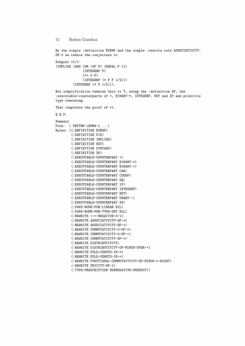
72 Ruben Gamboa
By the simple :definition EVENP and the simple :rewrite rule ASSOCIATIVITY-
OF-* we reduce the conjecture to
Subgoal *1/1’
(IMPLIES (AND (OR (ZP P) (EQUAL P 1))
(INTEGERP P)
(<= 0 P)
(INTEGERP (* P P 1/2)))
(INTEGERP (* P 1/2))).
But simplification reduces this to T, using the :definition ZP, the
:executable-counterparts of <, BINARY-*, INTEGERP, NOT and ZP and primitive
type reasoning.
That completes the proof of *1.
Q.E.D.
Summary
Form: ( DEFTHM LEMMA-1 ...)
Rules: ((:DEFINITION EVENP)
(:DEFINITION FIX)
(:DEFINITION IMPLIES)
(:DEFINITION NOT)
(:DEFINITION SYNTAXP)
(:DEFINITION ZP)
(:EXECUTABLE-COUNTERPART <)
(:EXECUTABLE-COUNTERPART BINARY-*)
(:EXECUTABLE-COUNTERPART BINARY-+)
(:EXECUTABLE-COUNTERPART CAR)
(:EXECUTABLE-COUNTERPART CONSP)
(:EXECUTABLE-COUNTERPART EQ)
(:EXECUTABLE-COUNTERPART IF)
(:EXECUTABLE-COUNTERPART INTEGERP)
(:EXECUTABLE-COUNTERPART NOT)
(:EXECUTABLE-COUNTERPART UNARY--)
(:EXECUTABLE-COUNTERPART ZP)
(:FAKE-RUNE-FOR-LINEAR NIL)
(:FAKE-RUNE-FOR-TYPE-SET NIL)
(:REWRITE <-+-NEGATIVE-0-1)
(:REWRITE ASSOCIATIVITY-OF-*)
(:REWRITE ASSOCIATIVITY-OF-+)
(:REWRITE COMMUTATIVITY-2-OF-*)
(:REWRITE COMMUTATIVITY-2-OF-+)
(:REWRITE COMMUTATIVITY-OF-*)
(:REWRITE DISTRIBUTIVITY)
(:REWRITE DISTRIBUTIVITY-OF-MINUS-OVER-+)
(:REWRITE FOLD-CONSTS-IN-*)
(:REWRITE FOLD-CONSTS-IN-+)
(:REWRITE FUNCTIONAL-COMMUTATIVITY-OF-MINUS-*-RIGHT)
(:REWRITE UNICITY-OF-1)
(:TYPE-PRESCRIPTION NONNEGATIVE-PRODUCT))
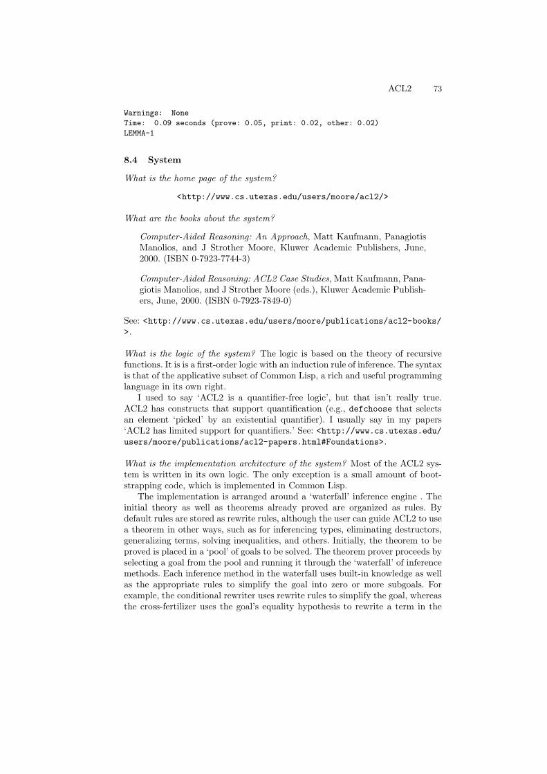
ACL2 73
Warnings: None
Time: 0.09 seconds (prove: 0.05, print: 0.02, other: 0.02)
LEMMA-1
8.4 System
What is the home page of the system?
<http://www.cs.utexas.edu/users/moore/acl2/>
What are the books about the system?
Computer-Aided Reasoning: An Approach, Matt Kaufmann, PanagiotisManolios, and J Strother Moore, Kluwer Academic Publishers, June,2000. (ISBN 0-7923-7744-3)
Computer-Aided Reasoning: ACL2 Case Studies, Matt Kaufmann, Pana-giotis Manolios, and J Strother Moore (eds.), Kluwer Academic Publish-ers, June, 2000. (ISBN 0-7923-7849-0)
See: <http://www.cs.utexas.edu/users/moore/publications/acl2-books/>.
What is the logic of the system? The logic is based on the theory of recursivefunctions. It is is a first-order logic with an induction rule of inference. The syntaxis that of the applicative subset of Common Lisp, a rich and useful programminglanguage in its own right.
I used to say ‘ACL2 is a quantifier-free logic’, but that isn’t really true.ACL2 has constructs that support quantification (e.g., defchoose that selectsan element ‘picked’ by an existential quantifier). I usually say in my papers‘ACL2 has limited support for quantifiers.’ See: <http://www.cs.utexas.edu/users/moore/publications/acl2-papers.html#Foundations>.
What is the implementation architecture of the system? Most of the ACL2 sys-tem is written in its own logic. The only exception is a small amount of boot-strapping code, which is implemented in Common Lisp.
The implementation is arranged around a ‘waterfall’ inference engine . Theinitial theory as well as theorems already proved are organized as rules. Bydefault rules are stored as rewrite rules, although the user can guide ACL2 to usea theorem in other ways, such as for inferencing types, eliminating destructors,generalizing terms, solving inequalities, and others. Initially, the theorem to beproved is placed in a ‘pool’ of goals to be solved. The theorem prover proceeds byselecting a goal from the pool and running it through the ‘waterfall’ of inferencemethods. Each inference method in the waterfall uses built-in knowledge as wellas the appropriate rules to simplify the goal into zero or more subgoals. Forexample, the conditional rewriter uses rewrite rules to simplify the goal, whereasthe cross-fertilizer uses the goal’s equality hypothesis to rewrite a term in the
74 Ruben Gamboa
goal, the generalizer uses generalization rules to prepare a theorem for induction,and the induction engine converts a goal into base and induction subgoals. If aninference method in the pool is successful, it removes the original goal from thepool and replaces it with the resulting subgoals. Note in particular that oncean inference method in the waterfall succeeds, none of the other methods areapplied to that goal.
What does working with the system look like? The user interacts with ACL2by submitting definitions and theorems. ACL2 responds with English text andformulas as its proof attempts progress. The user observes the output from failingproofs and typically formulates lemmas to submit to the system, generally in theform of rewrite rules (though many other rule types are supported), to ‘teach’ACL2 additional facts about the function symbols that have been introduced.Alternatively, the user may see a failed proof and decide to give ACL2 a hint(such as enabling or disabling certain rules, specifically requesting that a giveninstance of a rule be used in the proof, or suggesting a helpful induction scheme)to help it find the proof. The ultimate goal is to use ACL2 to ‘certify’ a collectionof ‘books’, each of which is a collection of ‘events’ (typically definitions andtheorems).
What is special about the system compared to other systems? ACL2 is being usedin at least two industrial settings on relatively large and difficult applications.Its prover heuristics are state-of-the-art for so-called inductive theorem provers,but perhaps more important is its robust engineering and extensive hyperlinkeddocumentation.
A compelling feature is that it is built around a real programming language.This makes it possible to develop a theory in ACL2 and execute it. This allowsthe user to debug the theory, as might be needed when formalizing a new systemfrom scratch. For example, after formalizing a microprocessor or a virtual ma-chine, it is possible to directly execute (i.e., simulate) a run of the microprocessoror VM, making it easier to find errors created in the modeling step before the(necessarily doomed) verification effort per se gets under way.
What are other versions of the system? Nqthm (aka the Boyer-Moore theoremprover) is a predecessor of ACL2 that uses a simpler, but very similar logic toACL2. Nqthm pioneered many of the techniques used in ACL2, such as thewaterfall design and the automatic discovery of induction schemes.
ACL2(r) is a variant of ACL2 that offers support for reasoning about theirrational real and complex numbers. It modifies the ACL2 logic by introducingnotions from non-standard analysis.
Who are the people behind the system? The authors are Matt Kaufmann andJ Moore, but Bob Boyer was also instrumental in the early development ofACL2. Many people have contributed to the improvement of ACL2, as de-scribed in the release notes <http://www.cs.utexas.edu/users/moore/acl2/v2-6/RELEASE-NOTES.html> and acknowledgments: <http://www.cs.utexas.edu/users/moore/acl2/v2-6/ACKNOWLEDGMENTS.html>.
ACL2 75
What are the main user communities of the system? There is a very active usercommunity in the University of Texas. In addition, there are active users inacademia all over the world, in Wyoming, Georgia, and Cadiz Spain. ACL2 hasalso found use in industrial settings, where it has been used to model, simulate,and verify various circuits and microprocessors. For example, it is in use at AMD,IBM, and Rockwell-Collins. Many people in the ACL2 community meet on oc-casion at ACL2 workshops. See: <http://www.cs.utexas.edu/users/moore/acl2/workshops.html>.
What large mathematical formalizations have been done in the system? ACL2has been used to prove a diverse set of results. For example, there are proofsconcerning the validity of micro-processor implementations of floating-point mul-tipliers and dividers, as well as transcendental functions like the floating-pointsquare root. There are ACL2 proofs verifying pipeline machines, parallel algo-rithms, and program translators. There are ACL2 formalizations of finite set the-ory, graph theory, and the Knuth-Bendix theorem. Other proofs include pieces ofreal analysis, such as the fundamental theorem of calculus, and Taylor’s theorem.
The results above merely scratch the surface. For a more complete list,see the ACL2 home page. See: <http://www.cs.utexas.edu/users/moore/
publications/acl2-papers.html>.
What representation of the formalization has been put in this paper? The rep-resentation of the proof is direct. The proof is based on the ACL2(r) variant ofACL2, although ACL2(r) is not needed until the last theorem, which uses thepredicate realp. ACL2(r) has built-in types for reals, rationals, integers, andcomplex numbers, and these are the only types used in the proof.
What needs to be explained about this specific proof? The last theorem is validonly in ACL2(r) and not ACL2. I.e., the predicate
(realp x)
does not exist in ACL2, since ACL2 only supports the rationals. ACL2(r) doessupport the reals, so the final statement is actually a theorem of ACL2(r) andnot ACL2. In plain old ACL2, you can prove the stronger result
[forall x] (not (equal (* x x) 2))
where the [forall x] is implied.
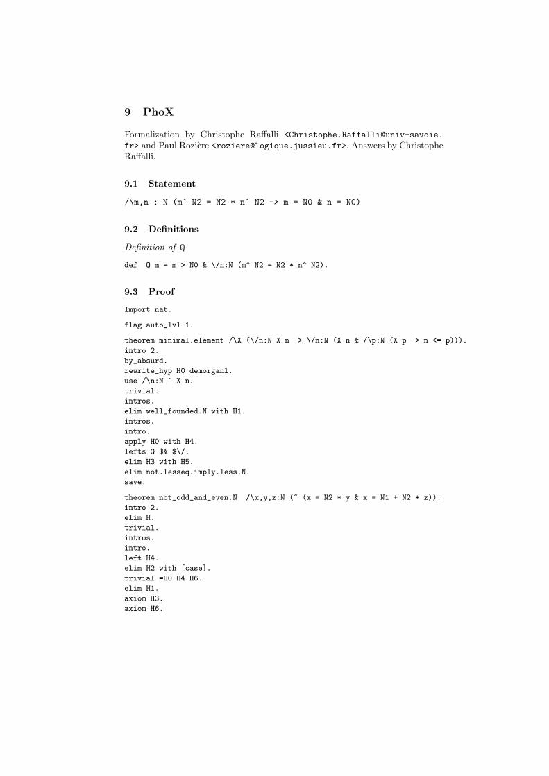
9 PhoX
Formalization by Christophe Raffalli <Christophe.Raffalli@univ-savoie.
fr> and Paul Roziere <[email protected]>. Answers by ChristopheRaffalli.
9.1 Statement
/\m,n : N (m^ N2 = N2 * n^ N2 -> m = N0 & n = N0)
9.2 Definitions
Definition of Q
def Q m = m > N0 & \/n:N (m^ N2 = N2 * n^ N2).
9.3 Proof
Import nat.
flag auto_lvl 1.
theorem minimal.element /\X (\/n:N X n -> \/n:N (X n & /\p:N (X p -> n <= p))).
intro 2.
by_absurd.
rewrite_hyp H0 demorganl.
use /\n:N ~ X n.
trivial.
intros.
elim well_founded.N with H1.
intros.
intro.
apply H0 with H4.
lefts G $& $\/.
elim H3 with H5.
elim not.lesseq.imply.less.N.
save.
theorem not_odd_and_even.N /\x,y,z:N (~ (x = N2 * y & x = N1 + N2 * z)).
intro 2.
elim H.
trivial.
intros.
intro.
left H4.
elim H2 with [case].
trivial =H0 H4 H6.
elim H1.
axiom H3.
axiom H6.
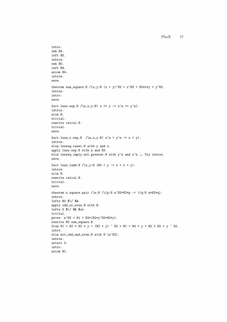
PhoX 77
intro.
rmh H4.
left H5.
intros.
rmh H5.
left H4.
axiom H4.
intros.
save.
theorem sum_square.N /\x,y:N (x + y)^N2 = x^N2 + N2*x*y + y^N2.
intros.
intro.
save.
fact less.exp.N /\n,x,y:N( x <= y -> x^n <= y^n).
intros.
elim H.
trivial.
rewrite calcul.N.
trivial.
save.
fact less_r.exp.N /\n,x,y:N( x^n < y^n -> x < y).
intros.
elim lesseq.case1.N with y and x.
apply less.exp.N with n and H3.
elim lesseq.imply.not.greater.N with y^n and x^n ;; Try intros.
save.
fact less.ladd.N /\x,y:N (N0 < y -> x < x + y).
intros.
elim H.
rewrite calcul.N.
trivial.
save.
theorem n.square.pair /\n:N (\/p:N n^N2=N2*p -> \/q:N n=N2*q).
intros.
lefts H0 $\/ $&.
apply odd_or_even.N with H.
lefts G $\/ $& $or.
trivial.
prove n^N2 = N1 + N2*(N2*y^N2+N2*y).
rewrite H3 sum_square.N.
from N1 + N2 * N2 * y + (N2 * y) ^ N2 = N1 + N4 * y + N2 * N2 * y ^ N2.
intro.
elim not_odd_and_even.N with N (n^N2).
intros.
select 3.
intro.
axiom H1.
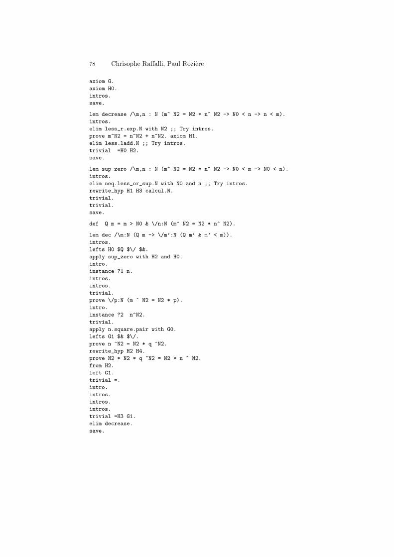
78 Chrisophe Raffalli, Paul Roziere
axiom G.
axiom H0.
intros.
save.
lem decrease /\m,n : N (m^ N2 = N2 * n^ N2 -> N0 < n -> n < m).
intros.
elim less_r.exp.N with N2 ;; Try intros.
prove m^N2 = n^N2 + n^N2. axiom H1.
elim less.ladd.N ;; Try intros.
trivial =H0 H2.
save.
lem sup_zero /\m,n : N (m^ N2 = N2 * n^ N2 -> N0 < m -> N0 < n).
intros.
elim neq.less_or_sup.N with N0 and n ;; Try intros.
rewrite_hyp H1 H3 calcul.N.
trivial.
trivial.
save.
def Q m = m > N0 & \/n:N (m^ N2 = N2 * n^ N2).
lem dec /\m:N (Q m -> \/m’:N (Q m’ & m’ < m)).
intros.
lefts H0 $Q $\/ $&.
apply sup_zero with H2 and H0.
intro.
instance ?1 n.
intros.
intros.
trivial.
prove \/p:N (m ^ N2 = N2 * p).
intro.
instance ?2 n^N2.
trivial.
apply n.square.pair with G0.
lefts G1 $& $\/.
prove n ^N2 = N2 * q ^N2.
rewrite_hyp H2 H4.
prove N2 * N2 * q ^N2 = N2 * n ^ N2.
from H2.
left G1.
trivial =.
intro.
intros.
intros.
intros.
trivial =H3 G1.
elim decrease.
save.
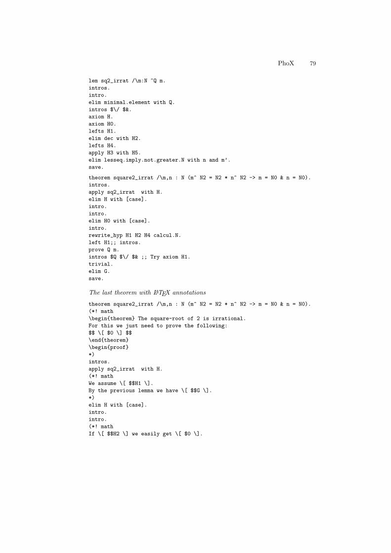
PhoX 79
lem sq2_irrat /\m:N ~Q m.
intros.
intro.
elim minimal.element with Q.
intros $\/ $&.
axiom H.
axiom H0.
lefts H1.
elim dec with H2.
lefts H4.
apply H3 with H5.
elim lesseq.imply.not.greater.N with n and m’.
save.
theorem square2_irrat /\m,n : N (m^ N2 = N2 * n^ N2 -> m = N0 & n = N0).
intros.
apply sq2_irrat with H.
elim H with [case].
intro.
intro.
elim H0 with [case].
intro.
rewrite_hyp H1 H2 H4 calcul.N.
left H1;; intros.
prove Q m.
intros $Q $\/ $& ;; Try axiom H1.
trivial.
elim G.
save.
The last theorem with LATEX annotations
theorem square2_irrat /\m,n : N (m^ N2 = N2 * n^ N2 -> m = N0 & n = N0).
(*! math
\begintheorem The square-root of 2 is irrational.
For this we just need to prove the following:
$$ \[ $0 \] $$
\endtheorem
\beginproof
*)
intros.
apply sq2_irrat with H.
(*! math
We assume \[ $$H1 \].
By the previous lemma we have \[ $$G \].
*)
elim H with [case].
intro.
intro.
(*! math
If \[ $$H2 \] we easily get \[ $0 \].
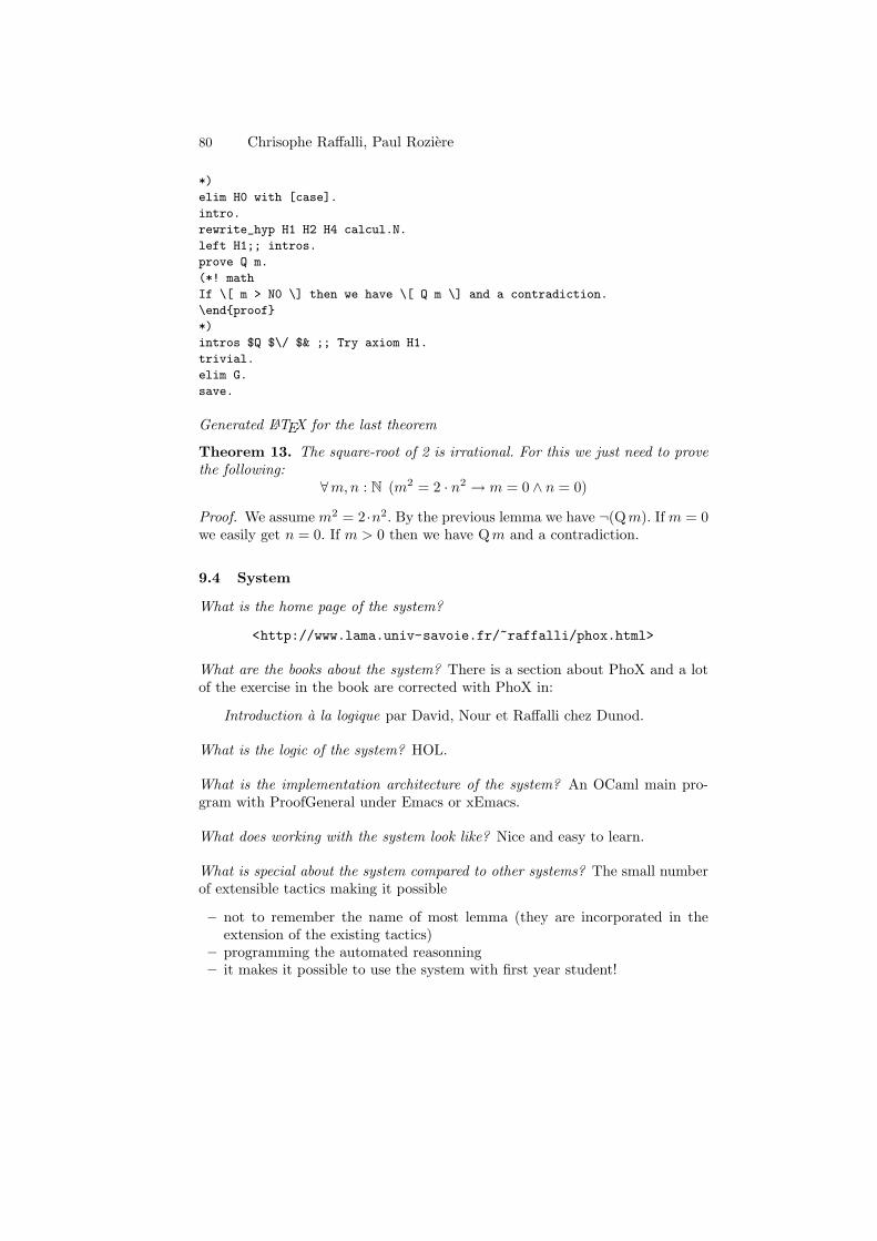
80 Chrisophe Raffalli, Paul Roziere
*)
elim H0 with [case].
intro.
rewrite_hyp H1 H2 H4 calcul.N.
left H1;; intros.
prove Q m.
(*! math
If \[ m > N0 \] then we have \[ Q m \] and a contradiction.
\endproof
*)
intros $Q $\/ $& ;; Try axiom H1.
trivial.
elim G.
save.
Generated LATEX for the last theorem
Theorem 13. The square-root of 2 is irrational. For this we just need to provethe following:
∀m,n : N (m2 = 2 · n2 → m = 0 ∧ n = 0)
Proof. We assume m2 = 2 ·n2. By the previous lemma we have ¬(Q m). If m = 0we easily get n = 0. If m > 0 then we have Qm and a contradiction.
9.4 System
What is the home page of the system?
<http://www.lama.univ-savoie.fr/~raffalli/phox.html>
What are the books about the system? There is a section about PhoX and a lotof the exercise in the book are corrected with PhoX in:
Introduction a la logique par David, Nour et Raffalli chez Dunod.
What is the logic of the system? HOL.
What is the implementation architecture of the system? An OCaml main pro-gram with ProofGeneral under Emacs or xEmacs.
What does working with the system look like? Nice and easy to learn.
What is special about the system compared to other systems? The small numberof extensible tactics making it possible
– not to remember the name of most lemma (they are incorporated in theextension of the existing tactics)
– programming the automated reasonning– it makes it possible to use the system with first year student!
PhoX 81
What are other versions of the system? None.
Who are the people behind the system? Mostly Christophe Raffalli, but also PaulRoziere (Paris VII) for some examples and part of the documentation.
What are the main user communities of the system? Math students from firstyear to PhD.
What large mathematical formalizations have been done in the system? Verylarge none, but interesting piece like arithmetic, Zorn and Zermelo from AC,Ramsey infinite theorem (n-uplet and k colors).
What representation of the formalization has been put in this paper? Tacticscript, plus example of annotation and generated latex.
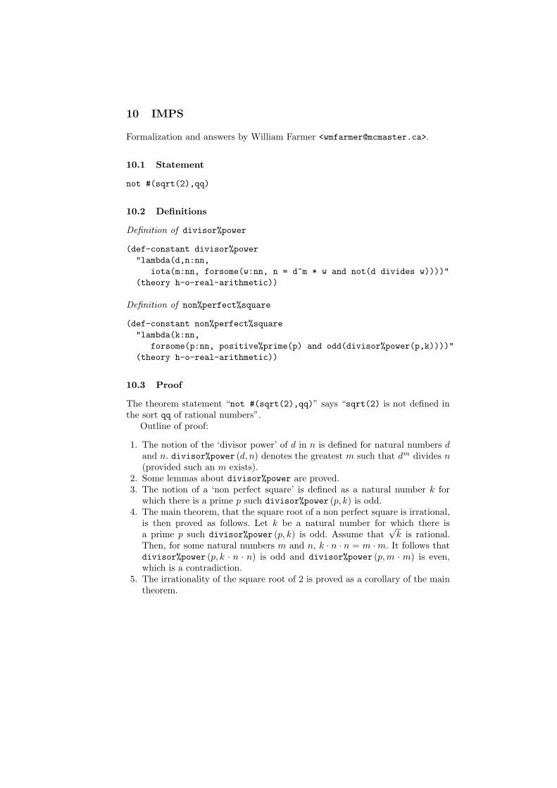
10 IMPS
Formalization and answers by William Farmer <[email protected]>.
10.1 Statement
not #(sqrt(2),qq)
10.2 Definitions
Definition of divisor%power
(def-constant divisor%power
"lambda(d,n:nn,
iota(m:nn, forsome(w:nn, n = d^m * w and not(d divides w))))"
(theory h-o-real-arithmetic))
Definition of non%perfect%square
(def-constant non%perfect%square
"lambda(k:nn,
forsome(p:nn, positive%prime(p) and odd(divisor%power(p,k))))"
(theory h-o-real-arithmetic))
10.3 Proof
The theorem statement “not #(sqrt(2),qq)” says “sqrt(2) is not defined inthe sort qq of rational numbers”.
Outline of proof:
1. The notion of the ‘divisor power’ of d in n is defined for natural numbers dand n. divisor%power (d, n) denotes the greatest m such that dm divides n(provided such an m exists).
2. Some lemmas about divisor%power are proved.3. The notion of a ‘non perfect square’ is defined as a natural number k for
which there is a prime p such divisor%power (p, k) is odd.4. The main theorem, that the square root of a non perfect square is irrational,
is then proved as follows. Let k be a natural number for which there isa prime p such divisor%power (p, k) is odd. Assume that
√k is rational.
Then, for some natural numbers m and n, k · n · n = m · m. It follows thatdivisor%power (p, k · n · n) is odd and divisor%power (p,m · m) is even,which is a contradiction.
5. The irrationality of the square root of 2 is proved as a corollary of the maintheorem.
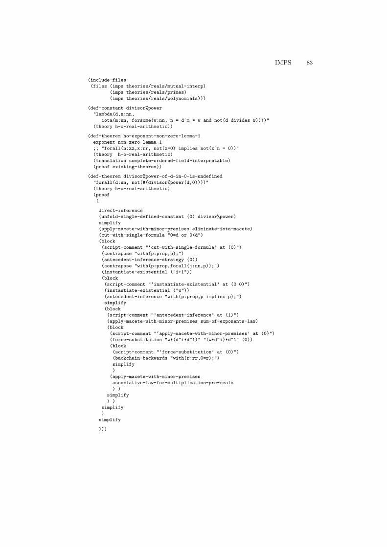
IMPS 83
(include-files
(files (imps theories/reals/mutual-interp)
(imps theories/reals/primes)
(imps theories/reals/polynomials)))
(def-constant divisor%power
"lambda(d,n:nn,
iota(m:nn, forsome(w:nn, n = d^m * w and not(d divides w))))"
(theory h-o-real-arithmetic))
(def-theorem ho-exponent-non-zero-lemma-1
exponent-non-zero-lemma-1
;; "forall(n:zz,x:rr, not(x=0) implies not(x^n = 0))"
(theory h-o-real-arithmetic)
(translation complete-ordered-field-interpretable)
(proof existing-theorem))
(def-theorem divisor%power-of-d-in-0-is-undefined
"forall(d:nn, not(#(divisor%power(d,0))))"
(theory h-o-real-arithmetic)
(proof
(
direct-inference
(unfold-single-defined-constant (0) divisor%power)
simplify
(apply-macete-with-minor-premises eliminate-iota-macete)
(cut-with-single-formula "0=d or 0<d")
(block
(script-comment "‘cut-with-single-formula’ at (0)")
(contrapose "with(p:prop,p);")
(antecedent-inference-strategy (0))
(contrapose "with(p:prop,forall(j:nn,p));")
(instantiate-existential ("i+1"))
(block
(script-comment "‘instantiate-existential’ at (0 0)")
(instantiate-existential ("w"))
(antecedent-inference "with(p:prop,p implies p);")
simplify
(block
(script-comment "‘antecedent-inference’ at (1)")
(apply-macete-with-minor-premises sum-of-exponents-law)
(block
(script-comment "‘apply-macete-with-minor-premises’ at (0)")
(force-substitution "w*(d^i*d^1)" "(w*d^i)*d^1" (0))
(block
(script-comment "‘force-substitution’ at (0)")
(backchain-backwards "with(r:rr,0=r);")
simplify
)
(apply-macete-with-minor-premises
associative-law-for-multiplication-pre-reals
) )
simplify
) )
simplify
)
simplify
)))
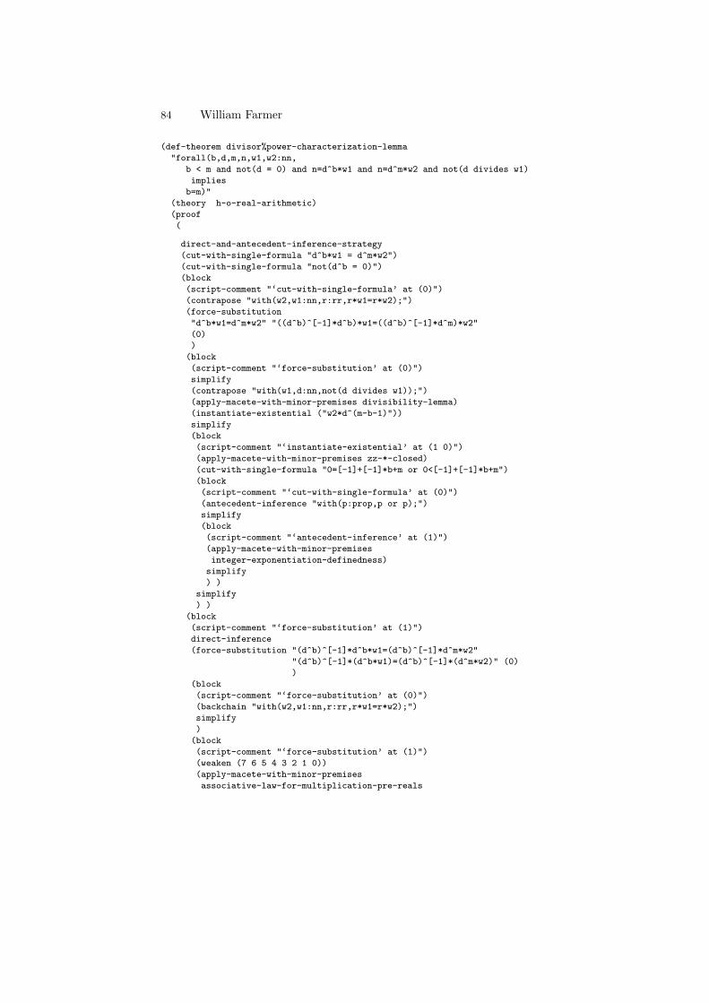
84 William Farmer
(def-theorem divisor%power-characterization-lemma
"forall(b,d,m,n,w1,w2:nn,
b < m and not(d = 0) and n=d^b*w1 and n=d^m*w2 and not(d divides w1)
implies
b=m)"
(theory h-o-real-arithmetic)
(proof
(
direct-and-antecedent-inference-strategy
(cut-with-single-formula "d^b*w1 = d^m*w2")
(cut-with-single-formula "not(d^b = 0)")
(block
(script-comment "‘cut-with-single-formula’ at (0)")
(contrapose "with(w2,w1:nn,r:rr,r*w1=r*w2);")
(force-substitution
"d^b*w1=d^m*w2" "((d^b)^[-1]*d^b)*w1=((d^b)^[-1]*d^m)*w2"
(0)
)
(block
(script-comment "‘force-substitution’ at (0)")
simplify
(contrapose "with(w1,d:nn,not(d divides w1));")
(apply-macete-with-minor-premises divisibility-lemma)
(instantiate-existential ("w2*d^(m-b-1)"))
simplify
(block
(script-comment "‘instantiate-existential’ at (1 0)")
(apply-macete-with-minor-premises zz-*-closed)
(cut-with-single-formula "0=[-1]+[-1]*b+m or 0<[-1]+[-1]*b+m")
(block
(script-comment "‘cut-with-single-formula’ at (0)")
(antecedent-inference "with(p:prop,p or p);")
simplify
(block
(script-comment "‘antecedent-inference’ at (1)")
(apply-macete-with-minor-premises
integer-exponentiation-definedness)
simplify
) )
simplify
) )
(block
(script-comment "‘force-substitution’ at (1)")
direct-inference
(force-substitution "(d^b)^[-1]*d^b*w1=(d^b)^[-1]*d^m*w2"
"(d^b)^[-1]*(d^b*w1)=(d^b)^[-1]*(d^m*w2)" (0)
)
(block
(script-comment "‘force-substitution’ at (0)")
(backchain "with(w2,w1:nn,r:rr,r*w1=r*w2);")
simplify
)
(block
(script-comment "‘force-substitution’ at (1)")
(weaken (7 6 5 4 3 2 1 0))
(apply-macete-with-minor-premises
associative-law-for-multiplication-pre-reals
IMPS 85
) ) ) )
(apply-macete-with-minor-premises ho-exponent-non-zero-lemma-1)
)))
(def-theorem divisor%power-characterization
"forall(d,n,m:nn,
not(d = 0)
implies
(m = divisor%power(d,n)
iff
forsome(w:nn, n = d^m * w and not(d divides w))))"
reverse
(theory h-o-real-arithmetic)
(proof
(
(unfold-single-defined-constant (0) divisor%power)
(apply-macete-with-minor-premises eliminate-iota-macete)
direct-and-antecedent-inference-strategy
(cut-with-single-formula "b<m or b=m or b>m")
(block
(script-comment "‘cut-with-single-formula’ at (0)")
(antecedent-inference "with(p:prop,p or p or p);")
(block
(script-comment "‘antecedent-inference’ at (0)")
(apply-macete-with-minor-premises
divisor%power-characterization-lemma)
auto-instantiate-existential
)
(block
(script-comment "‘antecedent-inference’ at (2)")
(force-substitution "b=m" "m=b" (0))
(block
(script-comment "‘force-substitution’ at (0)")
(apply-macete-with-minor-premises
divisor%power-characterization-lemma)
auto-instantiate-existential
(incorporate-antecedent "with(m,b:nn,b>m);")
(unfold-single-defined-constant (0) >)
)
simplify
) )
simplify
)))
(def-theorem divisor%power-is-almost-total-aux
"forall(d:nn,
2<=d
implies
forall(n:zz, 1<=n implies lambda(n1:zz, #(divisor%power(d,n1)))(n)))"
(theory h-o-real-arithmetic)
(proof
(
(apply-macete-with-minor-premises complete-induction-schema)
simplify
direct-and-antecedent-inference-strategy
(cut-with-single-formula "d divides m or not(d divides m)")
86 William Farmer
(block
(script-comment "‘cut-with-single-formula’ at (0)")
(antecedent-inference "with(p:prop,p or p);")
(block
(script-comment "‘antecedent-inference’ at (0)")
(incorporate-antecedent "with(m:zz,d:nn,d divides m);")
(apply-macete-with-minor-premises divisibility-lemma)
direct-and-antecedent-inference-strategy
(backchain "with(r:rr,m:zz,m=r);")
(cut-with-single-formula "1<=k and k<m")
(block
(script-comment "‘cut-with-single-formula’ at (0)")
(instantiate-universal-antecedent "with(p:prop,forall(k:zz,p));" ("k"))
(incorporate-antecedent "with(n:nn,#(n));")
(force-substitution "#(divisor%power(d,k))"
"forsome(m1:nn, m1=divisor%power(d,k))" (0)
)
(block
(script-comment "‘force-substitution’ at (0)")
(force-substitution "#(divisor%power(d,k*d))"
"forsome(m2:nn, m2=divisor%power(d,k*d))" (0)
)
(block
(script-comment "‘force-substitution’ at (0)")
(apply-macete-with-minor-premises divisor%power-characterization)
direct-and-antecedent-inference-strategy
(instantiate-existential ("m1+1"))
auto-instantiate-existential
(backchain "with(w,m1,d:nn,k:zz,k=d^m1*w);")
(force-substitution "d^m1*w*d" "d^m1*d*w" (0))
simplify
(block
(script-comment "‘force-substitution’ at (1)")
(force-substitution "d^m1*w*d" "d^m1*(w*d)" (0))
(block
(script-comment "‘force-substitution’ at (0)")
(apply-macete-locally-with-minor-premises
commutative-law-for-multiplication-pre-reals (0) "w*d"
)
(apply-macete-with-minor-premises
associative-law-for-multiplication-pre-reals
) )
(apply-macete-with-minor-premises
associative-law-for-multiplication-pre-reals
) ) )
simplify
)
simplify
)
(block
(script-comment "‘cut-with-single-formula’ at (1)")
direct-inference
(block
(script-comment "‘direct-inference’ at (0)")
(cut-with-single-formula "0<k or 0=k or k<0")
(block
(script-comment "‘cut-with-single-formula’ at (0)")
IMPS 87
(antecedent-inference "with(p:prop,p or p or p);")
simplify
(block
(script-comment "‘antecedent-inference’ at (1)")
(contrapose "with(d:nn,k,m:zz,m=k*d);")
simplify
)
(block
(script-comment "‘antecedent-inference’ at (2)")
(cut-with-single-formula "k*d<0")
(block
(script-comment "‘cut-with-single-formula’ at (0)")
(contrapose "with(r:rr,m:zz,m=r);")
simplify
)
(block
(script-comment "‘cut-with-single-formula’ at (1)")
(force-substitution "k*d" "d*k" (0))
(block
(script-comment "‘force-substitution’ at (0)")
(apply-macete-with-minor-premises
strict-negativity-for-products
)
simplify
)
simplify
) ) )
simplify
)
(block
(script-comment "‘direct-inference’ at (1)")
(backchain "with(r:rr,m:zz,m=r);")
(force-substitution "k*d" "d*k" (0))
simplify
simplify
) ) )
(block
(script-comment "‘antecedent-inference’ at (1 1 (1 . 0))")
(force-substitution "#(divisor%power(d,m))"
"forsome(m1:nn, m1=divisor%power(d,m))" (0)
)
(block
(script-comment "‘force-substitution’ at (0)")
(apply-macete-with-minor-premises divisor%power-characterization)
(instantiate-existential ("0"))
(instantiate-existential ("m"))
simplify
)
(block
(script-comment "‘force-substitution’ at nil")
(weaken (3 2 1 0))
simplify
) ) )
simplify
)))
(def-theorem divisor%power-is-almost-total
88 William Farmer
"forall(d,n:nn, 2 <= d and 1 <= n implies #(divisor%power(d,n)))"
(theory h-o-real-arithmetic)
(proof
(
direct-and-antecedent-inference-strategy
(instantiate-theorem divisor%power-is-almost-total-aux ("d"))
(incorporate-antecedent "with(p:prop,forall(n:zz,p));")
simplify
)))
(def-theorem divisor%power-sum-law
"forall(p,a,b:nn,
positive%prime(p) and 1 <= a and 1 <= b
implies
divisor%power(p,a*b) = divisor%power(p,a) + divisor%power(p,b))"
(theory h-o-real-arithmetic)
(proof
(
direct-and-antecedent-inference-strategy
(cut-with-single-formula "2<=p")
(block
(script-comment "‘cut-with-single-formula’ at (0)")
(cut-with-single-formula
"#(divisor%power(p,a)) and #(divisor%power(p,b))")
(block
(script-comment "‘cut-with-single-formula’ at (0)")
(antecedent-inference "with(p:prop,p and p);")
(cut-with-single-formula
"forsome(m1:nn,m1=divisor%power(p,a)) and
forsome(m2:nn,m2=divisor%power(p,b))"
)
(block
(script-comment "‘cut-with-single-formula’ at (0)")
(antecedent-inference-strategy (0))
(backchain-backwards "with(a,p,m1:nn,m1=divisor%power(p,a));")
(backchain-backwards "with(b,p,m2:nn,m2=divisor%power(p,b));")
(incorporate-antecedent "with(a,p,m1:nn,m1=divisor%power(p,a));")
(incorporate-antecedent "with(n,m2:nn,m2=n);")
(apply-macete-with-minor-premises divisor%power-characterization)
direct-and-antecedent-inference-strategy
(cut-with-single-formula "a*b=p^(m1+m2)*w*w_$0")
(block
(script-comment "‘cut-with-single-formula’ at (0)")
(cut-with-single-formula "not(p divides w*w_$0)")
(block
(script-comment "‘cut-with-single-formula’ at (0)")
(cut-with-single-formula
"forsome(w:nn, a*b = p^(m1+m2) * w and not(p divides w))"
)
(block
(script-comment "‘cut-with-single-formula’ at (0)")
(incorporate-antecedent "with(p:prop,forsome(w:nn,p));")
(apply-macete-with-minor-premises
rev%divisor%power-characterization
)
direct-inference
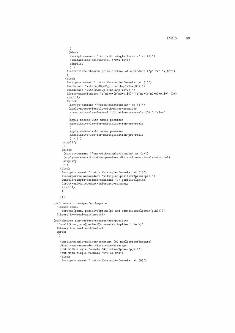
IMPS 89
)
(block
(script-comment "‘cut-with-single-formula’ at (1)")
(instantiate-existential ("w*w_$0"))
simplify
) )
(instantiate-theorem prime-divisor-of-a-product ("p" "w" "w_$0"))
)
(block
(script-comment "‘cut-with-single-formula’ at (1)")
(backchain "with(w_$0,m2,p,b:nn,b=p^m2*w_$0);")
(backchain "with(w,m1,p,a:nn,a=p^m1*w);")
(force-substitution "p^m1*w*(p^m2*w_$0)" "p^m1*(p^m2*w)*w_$0" (0))
simplify
(block
(script-comment "‘force-substitution’ at (1)")
(apply-macete-locally-with-minor-premises
commutative-law-for-multiplication-pre-reals (0) "p^m2*w"
)
(apply-macete-with-minor-premises
associative-law-for-multiplication-pre-reals
)
(apply-macete-with-minor-premises
associative-law-for-multiplication-pre-reals
) ) ) )
simplify
)
(block
(script-comment "‘cut-with-single-formula’ at (1)")
(apply-macete-with-minor-premises divisor%power-is-almost-total)
simplify
) )
(block
(script-comment "‘cut-with-single-formula’ at (1)")
(incorporate-antecedent "with(p:nn,positive%prime(p));")
(unfold-single-defined-constant (0) positive%prime)
direct-and-antecedent-inference-strategy
simplify
)
)))
(def-constant non%perfect%square
"lambda(k:nn,
forsome(p:nn, positive%prime(p) and odd(divisor%power(p,k))))"
(theory h-o-real-arithmetic))
(def-theorem non-perfect-squares-are-positive
"forall(k:nn, non%perfect%square(k) implies 1 <= k)"
(theory h-o-real-arithmetic)
(proof
(
(unfold-single-defined-constant (0) non%perfect%square)
direct-and-antecedent-inference-strategy
(cut-with-single-formula "#(divisor%power(p,k))")
(cut-with-single-formula "0=k or 0<k")
(block
(script-comment "‘cut-with-single-formula’ at (0)")
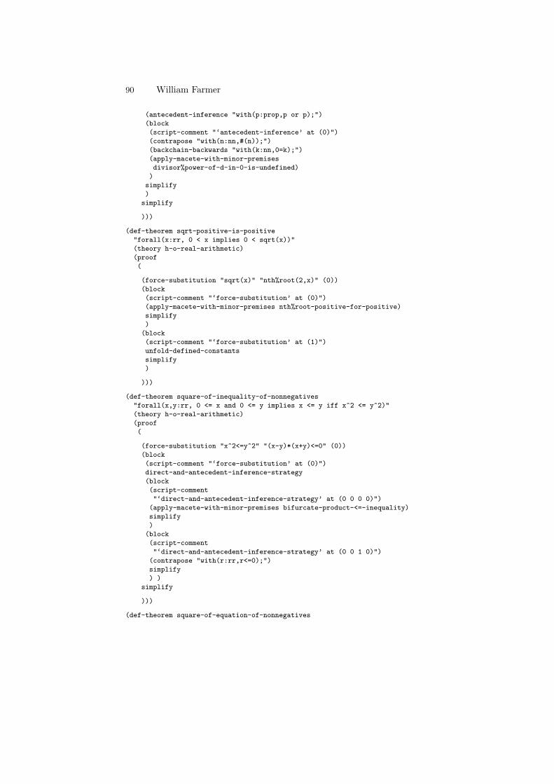
90 William Farmer
(antecedent-inference "with(p:prop,p or p);")
(block
(script-comment "‘antecedent-inference’ at (0)")
(contrapose "with(n:nn,#(n));")
(backchain-backwards "with(k:nn,0=k);")
(apply-macete-with-minor-premises
divisor%power-of-d-in-0-is-undefined)
)
simplify
)
simplify
)))
(def-theorem sqrt-positive-is-positive
"forall(x:rr, 0 < x implies 0 < sqrt(x))"
(theory h-o-real-arithmetic)
(proof
(
(force-substitution "sqrt(x)" "nth%root(2,x)" (0))
(block
(script-comment "‘force-substitution’ at (0)")
(apply-macete-with-minor-premises nth%root-positive-for-positive)
simplify
)
(block
(script-comment "‘force-substitution’ at (1)")
unfold-defined-constants
simplify
)
)))
(def-theorem square-of-inequality-of-nonnegatives
"forall(x,y:rr, 0 <= x and 0 <= y implies x <= y iff x^2 <= y^2)"
(theory h-o-real-arithmetic)
(proof
(
(force-substitution "x^2<=y^2" "(x-y)*(x+y)<=0" (0))
(block
(script-comment "‘force-substitution’ at (0)")
direct-and-antecedent-inference-strategy
(block
(script-comment
"‘direct-and-antecedent-inference-strategy’ at (0 0 0 0)")
(apply-macete-with-minor-premises bifurcate-product-<=-inequality)
simplify
)
(block
(script-comment
"‘direct-and-antecedent-inference-strategy’ at (0 0 1 0)")
(contrapose "with(r:rr,r<=0);")
simplify
) )
simplify
)))
(def-theorem square-of-equation-of-nonnegatives
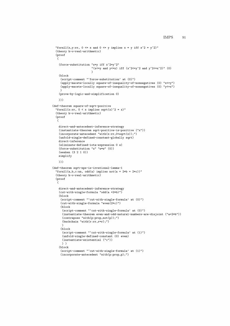
IMPS 91
"forall(x,y:rr, 0 <= x and 0 <= y implies x = y iff x^2 = y^2)"
(theory h-o-real-arithmetic)
(proof
(
(force-substitution "x=y iff x^2=y^2"
"(x<=y and y<=x) iff (x^2<=y^2 and y^2<=x^2)" (0)
)
(block
(script-comment "‘force-substitution’ at (0)")
(apply-macete-locally square-of-inequality-of-nonnegatives (0) "x<=y")
(apply-macete-locally square-of-inequality-of-nonnegatives (0) "y<=x")
)
(prove-by-logic-and-simplification 0)
)))
(def-theorem square-of-sqrt-positive
"forall(x:rr, 0 < x implies sqrt(x)^2 = x)"
(theory h-o-real-arithmetic)
(proof
(
direct-and-antecedent-inference-strategy
(instantiate-theorem sqrt-positive-is-positive ("x"))
(incorporate-antecedent "with(x:rr,0<sqrt(x));")
(unfold-single-defined-constant-globally sqrt)
direct-inference
(eliminate-defined-iota-expression 0 w)
(force-substitution "x" "w*w" (0))
(weaken (3 2 1 0))
simplify
)))
(def-theorem sqrt-nps-is-irrational-lemma-1
"forall(a,b,c:nn, odd(a) implies not(a + 2*b = 2*c))"
(theory h-o-real-arithmetic)
(proof
(
direct-and-antecedent-inference-strategy
(cut-with-single-formula "odd(a +2*b)")
(block
(script-comment "‘cut-with-single-formula’ at (0)")
(cut-with-single-formula "even(2*c)")
(block
(script-comment "‘cut-with-single-formula’ at (0)")
(instantiate-theorem even-and-odd-natural-numbers-are-disjoint ("a+2*b"))
(contrapose "with(p:prop,not(p));")
(backchain "with(r:rr,r=r);")
)
(block
(script-comment "‘cut-with-single-formula’ at (1)")
(unfold-single-defined-constant (0) even)
(instantiate-existential ("c"))
) )
(block
(script-comment "‘cut-with-single-formula’ at (1)")
(incorporate-antecedent "with(p:prop,p);")
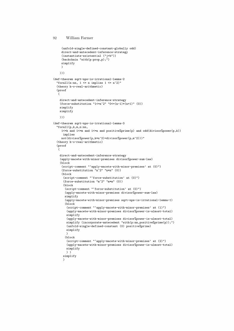
92 William Farmer
(unfold-single-defined-constant-globally odd)
direct-and-antecedent-inference-strategy
(instantiate-existential ("j+b"))
(backchain "with(p:prop,p);")
simplify
)
)))
(def-theorem sqrt-nps-is-irrational-lemma-2
"forall(n:nn, 1 <= n implies 1 <= n^2)"
(theory h-o-real-arithmetic)
(proof
(
direct-and-antecedent-inference-strategy
(force-substitution "1<=n^2" "0<=(n-1)*(n+1)" (0))
simplify
simplify
)))
(def-theorem sqrt-nps-is-irrational-lemma-3
"forall(p,k,m,n:nn,
1<=k and 1<=m and 1<=n and positive%prime(p) and odd(divisor%power(p,k))
implies
not(divisor%power(p,k*n^2)=divisor%power(p,m^2)))"
(theory h-o-real-arithmetic)
(proof
(
direct-and-antecedent-inference-strategy
(apply-macete-with-minor-premises divisor%power-sum-law)
(block
(script-comment "‘apply-macete-with-minor-premises’ at (0)")
(force-substitution "n^2" "n*n" (0))
(block
(script-comment "‘force-substitution’ at (0)")
(force-substitution "m^2" "m*m" (0))
(block
(script-comment "‘force-substitution’ at (0)")
(apply-macete-with-minor-premises divisor%power-sum-law)
simplify
(apply-macete-with-minor-premises sqrt-nps-is-irrational-lemma-1)
(block
(script-comment "‘apply-macete-with-minor-premises’ at (1)")
(apply-macete-with-minor-premises divisor%power-is-almost-total)
simplify
(apply-macete-with-minor-premises divisor%power-is-almost-total)
simplify (incorporate-antecedent "with(p:nn,positive%prime(p));")
(unfold-single-defined-constant (0) positive%prime)
simplify
)
(block
(script-comment "‘apply-macete-with-minor-premises’ at (2)")
(apply-macete-with-minor-premises divisor%power-is-almost-total)
simplify
) )
simplify
)
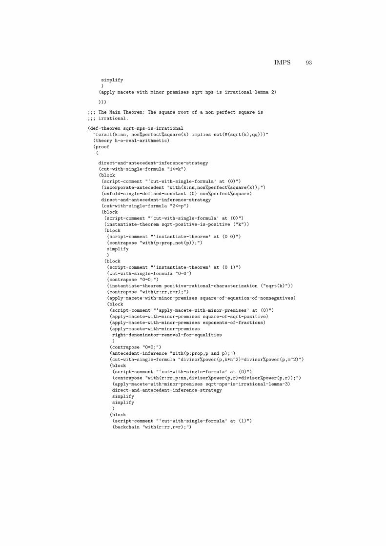
IMPS 93
simplify
)
(apply-macete-with-minor-premises sqrt-nps-is-irrational-lemma-2)
)))
;;; The Main Theorem: The square root of a non perfect square is
;;; irrational.
(def-theorem sqrt-nps-is-irrational
"forall(k:nn, non%perfect%square(k) implies not(#(sqrt(k),qq)))"
(theory h-o-real-arithmetic)
(proof
(
direct-and-antecedent-inference-strategy
(cut-with-single-formula "1<=k")
(block
(script-comment "‘cut-with-single-formula’ at (0)")
(incorporate-antecedent "with(k:nn,non%perfect%square(k));")
(unfold-single-defined-constant (0) non%perfect%square)
direct-and-antecedent-inference-strategy
(cut-with-single-formula "2<=p")
(block
(script-comment "‘cut-with-single-formula’ at (0)")
(instantiate-theorem sqrt-positive-is-positive ("k"))
(block
(script-comment "‘instantiate-theorem’ at (0 0)")
(contrapose "with(p:prop,not(p));")
simplify
)
(block
(script-comment "‘instantiate-theorem’ at (0 1)")
(cut-with-single-formula "0=0")
(contrapose "0=0;")
(instantiate-theorem positive-rational-characterization ("sqrt(k)"))
(contrapose "with(r:rr,r=r);")
(apply-macete-with-minor-premises square-of-equation-of-nonnegatives)
(block
(script-comment "‘apply-macete-with-minor-premises’ at (0)")
(apply-macete-with-minor-premises square-of-sqrt-positive)
(apply-macete-with-minor-premises exponents-of-fractions)
(apply-macete-with-minor-premises
right-denominator-removal-for-equalities
)
(contrapose "0=0;")
(antecedent-inference "with(p:prop,p and p);")
(cut-with-single-formula "divisor%power(p,k*n^2)=divisor%power(p,m^2)")
(block
(script-comment "‘cut-with-single-formula’ at (0)")
(contrapose "with(r:rr,p:nn,divisor%power(p,r)=divisor%power(p,r));")
(apply-macete-with-minor-premises sqrt-nps-is-irrational-lemma-3)
direct-and-antecedent-inference-strategy
simplify
simplify
)
(block
(script-comment "‘cut-with-single-formula’ at (1)")
(backchain "with(r:rr,r=r);")
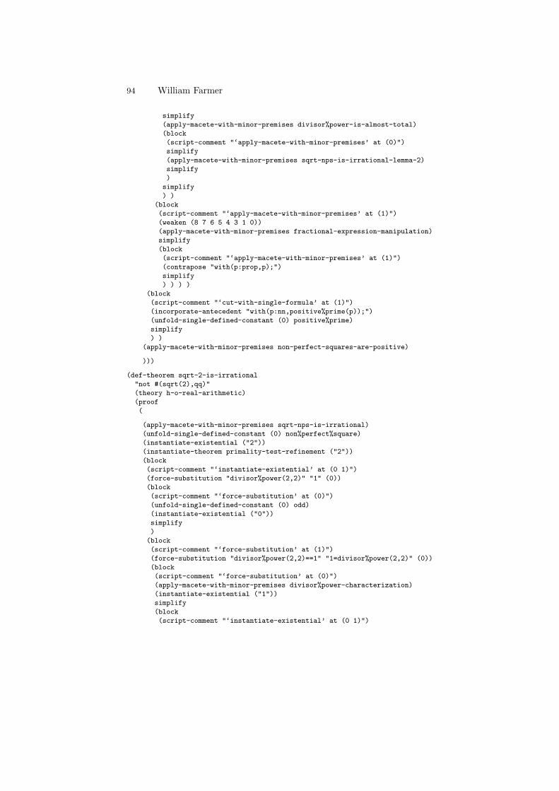
94 William Farmer
simplify
(apply-macete-with-minor-premises divisor%power-is-almost-total)
(block
(script-comment "‘apply-macete-with-minor-premises’ at (0)")
simplify
(apply-macete-with-minor-premises sqrt-nps-is-irrational-lemma-2)
simplify
)
simplify
) )
(block
(script-comment "‘apply-macete-with-minor-premises’ at (1)")
(weaken (8 7 6 5 4 3 1 0))
(apply-macete-with-minor-premises fractional-expression-manipulation)
simplify
(block
(script-comment "‘apply-macete-with-minor-premises’ at (1)")
(contrapose "with(p:prop,p);")
simplify
) ) ) )
(block
(script-comment "‘cut-with-single-formula’ at (1)")
(incorporate-antecedent "with(p:nn,positive%prime(p));")
(unfold-single-defined-constant (0) positive%prime)
simplify
) )
(apply-macete-with-minor-premises non-perfect-squares-are-positive)
)))
(def-theorem sqrt-2-is-irrational
"not #(sqrt(2),qq)"
(theory h-o-real-arithmetic)
(proof
(
(apply-macete-with-minor-premises sqrt-nps-is-irrational)
(unfold-single-defined-constant (0) non%perfect%square)
(instantiate-existential ("2"))
(instantiate-theorem primality-test-refinement ("2"))
(block
(script-comment "‘instantiate-existential’ at (0 1)")
(force-substitution "divisor%power(2,2)" "1" (0))
(block
(script-comment "‘force-substitution’ at (0)")
(unfold-single-defined-constant (0) odd)
(instantiate-existential ("0"))
simplify
)
(block
(script-comment "‘force-substitution’ at (1)")
(force-substitution "divisor%power(2,2)==1" "1=divisor%power(2,2)" (0))
(block
(script-comment "‘force-substitution’ at (0)")
(apply-macete-with-minor-premises divisor%power-characterization)
(instantiate-existential ("1"))
simplify
(block
(script-comment "‘instantiate-existential’ at (0 1)")
IMPS 95
(unfold-single-defined-constant (0) divides)
simplify
) )
simplify
) )
)))
10.4 System
What is the home page of the system?
http://imps.mcmaster.ca/
What are the books about the system? The best references for IMPS are:
J. D. Guttman, and F. J. Thayer, ‘IMPS: An Interactive MathematicalProof System’, Journal of Automated Reasoning, 11:213-248, 1993.
W. M. Farmer, J. D. Guttman, and F. J. Thayer, The IMPS User’sManual, Technical Report M-93B138, 289 pp., The MITRE Corporation,November 1993. Available at <http://imps.mcmaster.ca/manual/> or<http://imps.mcmaster.ca/doc/manual.pdf>.
What is the logic of the system? The logic of IMPS is LUTINS, a version ofChurch’s simple theory of types that admits undefined terms, partial functions,and subtypes. The following three papers collectively present the logic:
W. M. Farmer, ‘A Partial Functions Version of Church’s Simple Theoryof Types’, Journal of Symbolic Logic, 55:1269-1291, 1990.
W. M. Farmer, ‘A Simple Type Theory with Partial Functions and Sub-types’, Annals of Pure and Applied Logic, 64:211-240, 1993.
W. M. Farmer, ‘Theory Interpretation in Simple Type Theory’, in: J.Heering et al., eds., Higher-Order Algebra, Logic, and Term Rewrit-ing, Lecture Notes in Computer Science, vol. 816, pp. 96-123, Springer-Verlag, 1994.
What is the implementation architecture of the system? A running IMPS systemis composed of two intercommunicating processes: a Common Lisp IMPS processand an XEmacs user interface process. IMPS was originally written in the Tprogramming language. The original T code is executed in Common Lisp usinga partial macro/emulation of T.
What does working with the system look like? A running IMPS system consists ofan XEmacs window for interacting with IMPS and an Xdvi window for viewingexpressions and proofs. There are XEmacs buffers that show the Common Lispread-eval-print loop, the current deduction graph, the current subgoals, and theIMPS theory files in use.
96 William Farmer
What is special about the system compared to other systems? IMPS has severalunique characteristics:
– The logic admits undefined terms and partial functions but formulas arealways true or false. (References: See LUTINS papers above.)
– Proofs are a blend of computation and deduction. There are two main com-putation devices: (1) The IMPS simplifier performs automatic simplificationusing rewrite rules, algebraic simplification, and definedness checking. (2)The IMPS macete mechanism semiautomatically applies theorems to sub-goals. (References: See IMPS references above.)
– Mathematics is organized using the little theories version of the axiomaticmethod. In the little theories approach, reasoning is distributed over a net-work of theories linked by theory interpretations. The interpretations serve asconduits for passing information (in the form of theorems, definitions, etc.)from one theory to another. (References: W. M. Farmer, J. D. Guttman,and F. J. Thayer, ‘Little Theories’, in: D. Kapur, ed., Automated Deduc-tion – CADE-11, Lecture Notes in Computer Science, Vol. 607, pp. 567-581,Springer-Verlag, 1992.)
– A partial function may be defined by recursion as the least fixed point ofa monotone functional. A list of partial functions can be defined by mu-tual recursion via a list of monotone functions. (Reference: W. M. Farmer,‘A Scheme for Defining Partial Higher-Order Functions by Recursion’, in:A. Butterfield, ed., 3rd Irish Workshop on Formal Methods, 13 pp., elec-tronic Workshops in Computing, Springer-Verlag, <http://ewic.org.uk/ewic/workshop/view.cfm/IWFM-99>, 1999.)
– The IMPS logic LUTINS includes a definite description operator (instead ofa choice operator as found in other systems). Definite descriptions are quiteuseful for defining functions and other mathematical objects. (Reference: SeeIMPS User’s Manual above.)
– Proofs are represented as deduction graphs. Deduction graphs may containcycles and parallel attempts to solve a subgoal. (Reference: See IMPS User’sManual above.)
– IMPS employs a unique, pragmatic style of proof script for storing deductiongraphs, building tactics, and reusing parts of a deduction graph construction.(Reference: W. M. Farmer, J. D. Guttman, M. E. Nadel, and F. J. Thayer,‘Proof script pragmatics in IMPS’, in: A. Bundy, ed., Automated Deduction– CADE-12, Lecture Notes in Computer Science, Vol. 814, pp. 356 -370,Springer-Verlag, 1994.)
What are other versions of the system? Version 2.0 is currently the only sup-ported version of IMPS.
Who are the people behind the system? The developers of IMPS are WilliamM. Farmer (McMaster), Joshua D. Guttman (MITRE), and F. Javier Thayer(MITRE).
IMPS 97
What are the main user communities of the system? The two main user com-munities of IMPS are researchers at The MITRE Corporation and students atMcMaster University.
What large mathematical formalizations have been done in the system? TheIMPS theory library contains a large amount and variety of basic mathematicsincluding formalizations of the real number system and objects like sets andsequences; theories of abstract mathematical structures such as groups and met-ric spaces; and theories to support specific applications of IMPS in computerscience. Some example theorems proved in IMPS are:
– Banach contractive mapping fixed point theorem– Knaster fixed point theorem– Fundamental theorem of calculus– Fundamental counting theorem for group theory– Fundamental theorem of arithmetic
What representation of the formalization has been put in this paper? A formal-ization in IMPS consists of one or more IMPS library files. Each file containsa list of ‘def-forms’ for defining and modifying IMPS objects and for loadingsections of the IMPS library as well as individual library files. There are about30 kinds of def-forms. For example, there are def-forms for creating theories andinterpretations, installing definitions and theorems, and specifying the parse andprint syntax of formal symbols.
A user can create an IMPS library file by simply typing the desired def-forms.In practice, however, a user will usually add a def-form to a library file as follows.The user will select a location in the file and then select the desired kind of def-form to place there from a menu. The IMPS user interface will place a templateof the selected def-form at the selected location in the file. Finally, the user willfill in the template as desired. The def-form for installing a theorem containsa proof script, which is a list of proof command and control statements that,when executed, will create a proof in the form of an IMPS deduction graph. Theproof script in a theorem def-form is normally generated automatically from adeduction graph that the user has created interactively.
What needs to be explained about this specific proof?
– divisor%power is defined using iota, the IMPS definite description opera-tor.
– sqrt and divisor%power are strictly partial functions.– The irrationality of the square root of a non perfect square is expressed as a
sort definedness statement.– Some theorems from the theory complete-ordered-field are used in the
theory h-o-real-arithmetic via an interpretation from complete-or-
dered-field to h-o-real-arithmetic.
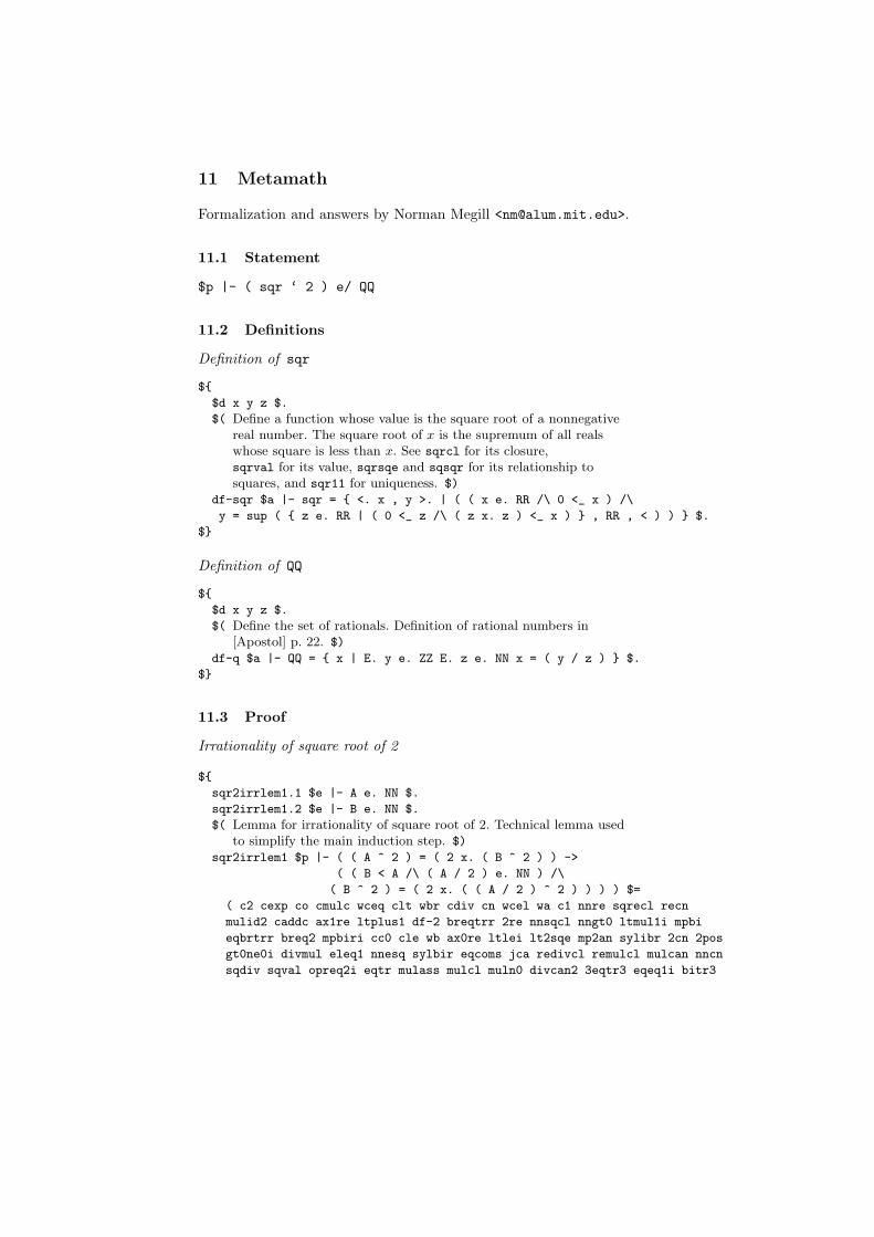
11 Metamath
Formalization and answers by Norman Megill <[email protected]>.
11.1 Statement
$p |- ( sqr ‘ 2 ) e/ QQ
11.2 Definitions
Definition of sqr
$
$d x y z $.
$( Define a function whose value is the square root of a nonnegativereal number. The square root of x is the supremum of all realswhose square is less than x. See sqrcl for its closure,sqrval for its value, sqrsqe and sqsqr for its relationship tosquares, and sqr11 for uniqueness. $)
df-sqr $a |- sqr = <. x , y >. | ( ( x e. RR /\ 0 <_ x ) /\
y = sup ( z e. RR | ( 0 <_ z /\ ( z x. z ) <_ x ) , RR , < ) ) $.
$
Definition of QQ
$
$d x y z $.
$( Define the set of rationals. Definition of rational numbers in[Apostol] p. 22. $)
df-q $a |- QQ = x | E. y e. ZZ E. z e. NN x = ( y / z ) $.
$
11.3 Proof
Irrationality of square root of 2
$
sqr2irrlem1.1 $e |- A e. NN $.
sqr2irrlem1.2 $e |- B e. NN $.
$( Lemma for irrationality of square root of 2. Technical lemma usedto simplify the main induction step. $)
sqr2irrlem1 $p |- ( ( A ^ 2 ) = ( 2 x. ( B ^ 2 ) ) ->
( ( B < A /\ ( A / 2 ) e. NN ) /\
( B ^ 2 ) = ( 2 x. ( ( A / 2 ) ^ 2 ) ) ) ) $=
( c2 cexp co cmulc wceq clt wbr cdiv cn wcel wa c1 nnre sqrecl recn
mulid2 caddc ax1re ltplus1 df-2 breqtrr 2re nnsqcl nngt0 ltmul1i mpbi
eqbrtrr breq2 mpbiri cc0 cle wb ax0re ltlei lt2sqe mp2an sylibr 2cn 2pos
gt0ne0i divmul eleq1 nnesq sylbir eqcoms jca redivcl remulcl mulcan nncn
sqdiv sqval opreq2i eqtr mulass mulcl muln0 divcan2 3eqtr3 eqeq1i bitr3
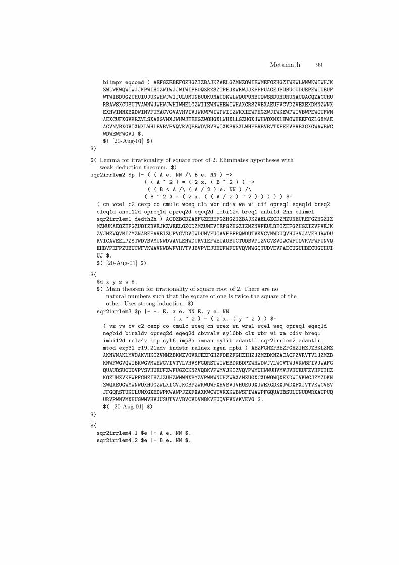
Metamath 99
biimpr eqcomd ) AEFGZEBEFGZHGZIZBAJKZAELGZMNZOWIEWMEFGZHGZIWKWLWNWKWIWHJK
ZWLWKWQWIWJJKPWIHGZWIWJJWIWIBBDQZRZSZTPEJKWRWJJKPPPUAGEJPUBUCUDUEPEWIUBUF
WTWIBDUGZUHUIUJUKWHWJWIJULUMUNBUOKUNAUOKWLWQUPUNBUQWSBDUHURUNAUQACQZACUHU
RBAWSXCUSUTVAWNWJWHWJWHIWHELGZWIIZWNWHEWIWHAXCRSZVBXAEUFVCVDZVEXEXDMNZWNX
EXHWIMNXBXDWIMVFUMACVGVAVHVIVJWKWPWIWPWIIZWKXIEWPHGZWJIWKEWPWIVBWPEWOUFWM
AEXCUFXGVKRZVLSXAXGVMXJWHWJEEHGZWOHGXLWHXLLGZHGXJWHWOXMXLHWOWHEEFGZLGXMAE
ACVNVBXGVOXNXLWHLEVBVPVQVRVQEEWOVBVBWOXKSVSXLWHEEVBVBVTXFEEVBVBXGXGWAWBWC
WDWEWFWGVJ $.
$( [20-Aug-01] $)
$
$( Lemma for irrationality of square root of 2. Eliminates hypotheses withweak deduction theorem. $)
sqr2irrlem2 $p |- ( ( A e. NN /\ B e. NN ) ->
( ( A ^ 2 ) = ( 2 x. ( B ^ 2 ) ) ->
( ( B < A /\ ( A / 2 ) e. NN ) /\
( B ^ 2 ) = ( 2 x. ( ( A / 2 ) ^ 2 ) ) ) ) ) $=
( cn wcel c2 cexp co cmulc wceq clt wbr cdiv wa wi cif opreq1 eqeq1d breq2
eleq1d anbi12d opreq1d opreq2d eqeq2d imbi12d breq1 anbi1d 2nn elimel
sqr2irrlem1 dedth2h ) ACDZBCDZAEFGZEBEFGZHGZIZBAJKZAELGZCDZMZUNEUREFGZHGZIZ
MZNUKAEOZEFGZUOIZBVEJKZVEELGZCDZMZUNEVIEFGZHGZIZMZNVFEULBEOZEFGZHGZIZVPVEJK
ZVJMZVQVMIZMZNABEEAVEIZUPVGVDVOWDUMVFUOAVEEFPQWDUTVKVCVNWDUQVHUSVJAVEBJRWDU
RVICAVEELPZSTWDVBVMUNWDVAVLEHWDURVIEFWEUAUBUCTUDBVPIZVGVSVOWCWFUOVRVFWFUNVQ
EHBVPEFPZUBUCWFVKWAVNWBWFVHVTVJBVPVEJUEUFWFUNVQVMWGQTUDVEVPAECUGUHBECUGUHUI
UJ $.
$( [20-Aug-01] $)
$
$d x y z w $.
$( Main theorem for irrationality of square root of 2. There are nonatural numbers such that the square of one is twice the square of theother. Uses strong induction. $)
sqr2irrlem3 $p |- -. E. x e. NN E. y e. NN
( x ^ 2 ) = ( 2 x. ( y ^ 2 ) ) $=
( vz vw cv c2 cexp co cmulc wceq cn wrex wn wral wcel weq opreq1 eqeq1d
negbid biraldv opreq2d eqeq2d cbvralv syl6bb clt wbr wi wa cdiv breq1
imbi12d rcla4v imp syl6 imp3a imnan sylib adantll sqr2irrlem2 adantlr
mtod exp31 r19.21adv indstr ralnex rgen mpbi ) AEZFGHZFBEZFGHZIHZJZBKLZMZ
AKNVNAKLMVOAKVHKOZVMMZBKNZVOVRCEZFGHZFDEZFGHZIHZJZMZDKNZACACPZVRVTVLJZMZB
KNWFWGVQWIBKWGVMWHWGVIVTVLVHVSFGQRSTWIWEBDKBDPZWHWDWJVLWCVTWJVKWBFIVJWAFG
QUAUBSUCUDVPVSVHUEUFZWFUGZCKNZVQBKVPWMVJKOZVQVPWMUHWNUHVMVJVHUEUFZVHFUIHZ
KOZUHZVKFWPFGHZIHZJZUHZWMWNXBMZVPWMWNUHZWRXAMZUGXCXDWOWQXEXDWOVKWCJZMZDKN
ZWQXEUGWMWNWOXHUGZWLXICVJKCBPZWKWOWFXHVSVJVHUEUJXJWEXGDKXJWDXFXJVTVKWCVSV
JFGQRSTUKULUMXGXEDWPKWAWPJZXFXAXKWCWTVKXKWBWSFIWAWPFGQUAUBSULUNUOWRXAUPUQ
URVPWNVMXBUGWMVHVJUSUTVAVBVCVDVMBKVEUQVFVNAKVEVG $.
$( [20-Aug-01] $)
$
$
sqr2irrlem4.1 $e |- A e. NN $.
sqr2irrlem4.2 $e |- B e. NN $.

100 Norman Megill
$( Lemma for irrationality of square root of 2. $)
sqr2irrlem4 $p |- ( ( sqr ‘ 2 ) = ( A / B ) <->
( A ^ 2 ) = ( 2 x. ( B ^ 2 ) ) ) $=
( c2 cexp co cmulc wceq csqr cfv cdiv nncn nnne0 sqdiv eqcomi nnsqcl 2cn
divcan4 eqeq12i nnre sqrecl recn 2re remulcl div11 eqcom 3bitr3 cc0 cle
wbr wb ax0re 2pos ltlei redivcl sqege0 sqr11 mp2an bitr4 nngt0 divgt0i
sqrsqe ax-mp eqeq2i bitr2 ) AEFGZEBEFGZHGZIZEJKZABLGZEFGZJKZIZVKVLIVJEVMI
ZVOVGVHLGZVIVHLGZIVMEIVJVPVQVMVREVMVQABACMBDMBDNZOPVHEVHBDQZMZRVHVTNZSTVG
VIVHVGAACUAZUBUCVIEVHUDVHVTUAUEUCWAWBUFVMEUGUHUIEUJUKUIVMUJUKVOVPULUIEUMU
DUNUOVLABWCBDUAZVSUPZUQEVMUDVLWEUBURUSUTVNVLVKUIVLUJUKVNVLIUIVLUMWEABWCWD
ACVABDVAVBUOVLWEVCVDVEVF $.
$( [20-Aug-01] $)
$
$( Lemma for irrationality of square root of 2. Eliminates hypotheses withweak deduction theorem. $)
sqr2irrlem5 $p |- ( ( A e. NN /\ B e. NN ) -> ( ( sqr ‘ 2 ) = ( A / B )
<-> ( A ^ 2 ) = ( 2 x. ( B ^ 2 ) ) ) ) $=
( cn wcel c2 csqr cfv cdiv co wceq cexp cmulc wb cif opreq1 eqeq2d eqeq1d
bibi12d opreq2 opreq2d 2nn elimel sqr2irrlem4 dedth2h ) ACDZBCDZEFGZABHIZJZ
AEKIZEBEKIZLIZJZMUGUEAENZBHIZJZUNEKIZULJZMUGUNUFBENZHIZJZUQEUSEKIZLIZJZMABE
EAUNJZUIUPUMURVEUHUOUGAUNBHOPVEUJUQULAUNEKOQRBUSJZUPVAURVDVFUOUTUGBUSUNHSPV
FULVCUQVFUKVBELBUSEKOTPRUNUSAECUAUBBECUAUBUCUD $.
$( [20-Aug-01] $)
$
$d x y $.
$( The square root of 2 is irrational. $)
sqr2irr $p |- ( sqr ‘ 2 ) e/ QQ $=
( vx vy c2 csqr cfv cq wnel wcel wn cv cdiv co wceq cn wrex cz cexp
cmulc sqr2irrlem3 sqr2irrlem5 bi2rexa mtbir cc0 clt wbr wa wi wb nngt0t
adantr cr ax0re ltmuldivt mp3an1 nnret zret syl2an mpd ancoms 2re 2pos
sqrgt0i breq2 mpbii syl5bir cc nncnt mulzer2t syl breq1d adantl sylibd
exp r19.23adv anc2li elnnz syl6ibr impac r19.22i2 mto elq df-nel mpbir )
CDEZFGWDFHZIWEWDAJZBJZKLZMZBNOZAPOZWKWJANOZWLWFCQLCWGCQLRLMZBNOANOABSWIWM
ABNNWFWGTUAUBWJWJAPNWFPHZWJWFNHZWNWJWNUCWFUDUEZUFWOWNWJWPWNWIWPBNWNWGNHZW
IWPUGWNWQUFZWIUCWGRLZWFUDUEZWPWRWTUCWHUDUEZWIWQWNWTXAUHZWQWNUFUCWGUDUEZXB
WQXCWNWGUIUJWGUKHZWFUKHZXCXBUGZWQWNUCUKHXDXEXFULUCWGWFUMUNWGUOWFUPUQURUSW
IUCWDUDUEXACUTVAVBWDWHUCUDVCVDVEWQWTWPUHWNWQWSUCWFUDWQWGVFHWSUCMWGVGWGVHV
IVJVKVLVMVNVOWFVPVQVRVSVTABWDWAUBWDFWBWC $.
$( [8-Jan-02] $)
$
Steps in the proof of the last theorem
51 mtbir.1=sqr2irrlem3 $p |- -. E. x e. NN E. y e. NN ( x ^ 2 ) = (
2 x. ( y ^ 2 ) )
60 bi2rexa.1=sqr2irrlem5 $p |- ( ( x e. NN /\ y e. NN ) -> ( ( sqr ‘
2 ) = ( x / y ) <-> ( x ^ 2 ) = ( 2 x. ( y ^ 2 ) ) ) )
61 mtbir.2=bi2rexa $p |- ( E. x e. NN E. y e. NN ( sqr ‘ 2 ) = (
x / y ) <-> E. x e. NN E. y e. NN ( x ^ 2 ) = ( 2 x. ( y ^ 2 ) ) )
62 mto.1=mtbir $p |- -. E. x e. NN E. y e. NN ( sqr ‘ 2 ) = (
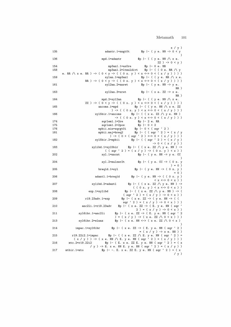
Metamath 101
x / y )
135 adantr.1=nngt0t $p |- ( y e. NN -> 0 < y
)
136 mpd.1=adantr $p |- ( ( y e. NN /\ x e.
ZZ ) -> 0 < y )
154 mp3an1.1=ax0re $p |- 0 e. RR
158 mp3an1.2=ltmuldivt $p |- ( ( 0 e. RR /\ y
e. RR /\ x e. RR ) -> ( 0 < y -> ( ( 0 x. y ) < x <-> 0 < ( x / y ) ) ) )
159 sylan.1=mp3an1 $p |- ( ( y e. RR /\ x e.
RR ) -> ( 0 < y -> ( ( 0 x. y ) < x <-> 0 < ( x / y ) ) ) )
161 syl2an.2=nnret $p |- ( y e. NN -> y e.
RR )
163 syl2an.3=zret $p |- ( x e. ZZ -> x e.
RR )
164 mpd.2=syl2an $p |- ( ( y e. NN /\ x e.
ZZ ) -> ( 0 < y -> ( ( 0 x. y ) < x <-> 0 < ( x / y ) ) ) )
165 ancoms.1=mpd $p |- ( ( y e. NN /\ x e. ZZ
) -> ( ( 0 x. y ) < x <-> 0 < ( x / y ) ) )
166 syl5bir.1=ancoms $p |- ( ( x e. ZZ /\ y e. NN )
-> ( ( 0 x. y ) < x <-> 0 < ( x / y ) ) )
174 sqrlem1.1=2re $p |- 2 e. RR
175 sqrlem1.2=2pos $p |- 0 < 2
176 mpbii.min=sqrgt0i $p |- 0 < ( sqr ‘ 2 )
181 mpbii.maj=breq2 $p |- ( ( sqr ‘ 2 ) = ( x / y
) -> ( 0 < ( sqr ‘ 2 ) <-> 0 < ( x / y ) ) )
182 syl5bir.2=mpbii $p |- ( ( sqr ‘ 2 ) = ( x / y )
-> 0 < ( x / y ) )
183 sylibd.1=syl5bir $p |- ( ( x e. ZZ /\ y e. NN ) ->
( ( sqr ‘ 2 ) = ( x / y ) -> ( 0 x. y ) < x ) )
202 syl.1=nncnt $p |- ( y e. NN -> y e. CC
)
204 syl.2=mulzer2t $p |- ( y e. CC -> ( 0 x. y
) = 0 )
205 breq1d.1=syl $p |- ( y e. NN -> ( 0 x. y )
= 0 )
206 adantl.1=breq1d $p |- ( y e. NN -> ( ( 0 x. y )
< x <-> 0 < x ) )
207 sylibd.2=adantl $p |- ( ( x e. ZZ /\ y e. NN ) ->
( ( 0 x. y ) < x <-> 0 < x ) )
208 exp.1=sylibd $p |- ( ( x e. ZZ /\ y e. NN ) -> (
( sqr ‘ 2 ) = ( x / y ) -> 0 < x ) )
209 r19.23adv.1=exp $p |- ( x e. ZZ -> ( y e. NN -> ( (
sqr ‘ 2 ) = ( x / y ) -> 0 < x ) ) )
210 anc2li.1=r19.23adv $p |- ( x e. ZZ -> ( E. y e. NN ( sqr ‘
2 ) = ( x / y ) -> 0 < x ) )
211 syl6ibr.1=anc2li $p |- ( x e. ZZ -> ( E. y e. NN ( sqr ‘ 2
) = ( x / y ) -> ( x e. ZZ /\ 0 < x ) ) )
213 syl6ibr.2=elnnz $p |- ( x e. NN <-> ( x e. ZZ /\ 0 < x )
)
214 impac.1=syl6ibr $p |- ( x e. ZZ -> ( E. y e. NN ( sqr ‘ 2 )
= ( x / y ) -> x e. NN ) )
215 r19.22i2.1=impac $p |- ( ( x e. ZZ /\ E. y e. NN ( sqr ‘ 2 ) =
( x / y ) ) -> ( x e. NN /\ E. y e. NN ( sqr ‘ 2 ) = ( x / y ) ) )
216 mto.2=r19.22i2 $p |- ( E. x e. ZZ E. y e. NN ( sqr ‘ 2 ) = ( x
/ y ) -> E. x e. NN E. y e. NN ( sqr ‘ 2 ) = ( x / y ) )
217 mtbir.1=mto $p |- -. E. x e. ZZ E. y e. NN ( sqr ‘ 2 ) = ( x
/ y )
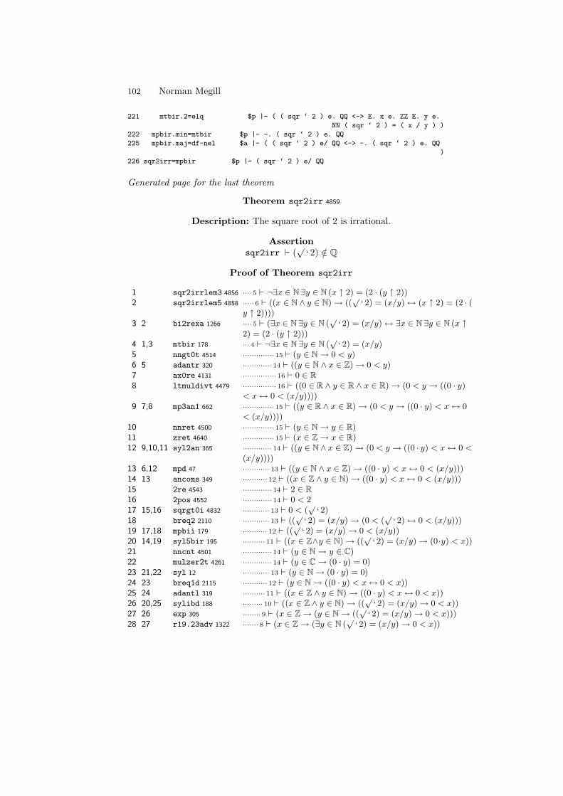
102 Norman Megill
221 mtbir.2=elq $p |- ( ( sqr ‘ 2 ) e. QQ <-> E. x e. ZZ E. y e.
NN ( sqr ‘ 2 ) = ( x / y ) )
222 mpbir.min=mtbir $p |- -. ( sqr ‘ 2 ) e. QQ
225 mpbir.maj=df-nel $a |- ( ( sqr ‘ 2 ) e/ QQ <-> -. ( sqr ‘ 2 ) e. QQ
)
226 sqr2irr=mpbir $p |- ( sqr ‘ 2 ) e/ QQ
Generated page for the last theorem
Theorem sqr2irr 4859
Description: The square root of 2 is irrational.
Assertionsqr2irr ` (
√‘ 2) /∈ Q
Proof of Theorem sqr2irr
1 sqr2irrlem3 4856 ···· 5 ` ¬∃x ∈ N∃y ∈ N (x ↑ 2) = (2 · (y ↑ 2))2 sqr2irrlem5 4858 ····· 6 ` ((x ∈ N ∧ y ∈ N) → ((
√‘ 2) = (x/y) ↔ (x ↑ 2) = (2 · (
y ↑ 2))))3 2 bi2rexa 1266 ···· 5 ` (∃x ∈ N∃y ∈ N (
√‘ 2) = (x/y) ↔ ∃x ∈ N∃y ∈ N (x ↑
2) = (2 · (y ↑ 2)))4 1,3 mtbir 178 ··· 4 ` ¬∃x ∈ N∃y ∈ N (
√‘ 2) = (x/y)
5 nngt0t 4514 ·············· 15 ` (y ∈ N → 0 < y)6 5 adantr 320 ············· 14 ` ((y ∈ N ∧ x ∈ Z) → 0 < y)7 ax0re 4131 ··············· 16 ` 0 ∈ R
8 ltmuldivt 4479 ··············· 16 ` ((0 ∈ R ∧ y ∈ R ∧ x ∈ R) → (0 < y → ((0 · y)< x ↔ 0 < (x/y))))
9 7,8 mp3an1 662 ·············· 15 ` ((y ∈ R ∧ x ∈ R) → (0 < y → ((0 · y) < x ↔ 0< (x/y))))
10 nnret 4500 ·············· 15 ` (y ∈ N → y ∈ R)11 zret 4640 ·············· 15 ` (x ∈ Z → x ∈ R)12 9,10,11 syl2an 365 ············· 14 ` ((y ∈ N∧ x ∈ Z) → (0 < y → ((0 · y) < x ↔ 0 <
(x/y))))13 6,12 mpd 47 ············ 13 ` ((y ∈ N ∧ x ∈ Z) → ((0 · y) < x ↔ 0 < (x/y)))14 13 ancoms 349 ··········· 12 ` ((x ∈ Z ∧ y ∈ N) → ((0 · y) < x ↔ 0 < (x/y)))15 2re 4543 ············· 14 ` 2 ∈ R
16 2pos 4552 ············· 14 ` 0 < 217 15,16 sqrgt0i 4832 ············ 13 ` 0 < (
√‘ 2)
18 breq2 2110 ············ 13 ` ((√
‘ 2) = (x/y) → (0 < (√
‘ 2) ↔ 0 < (x/y)))19 17,18 mpbii 179 ··········· 12 ` ((
√‘ 2) = (x/y) → 0 < (x/y))
20 14,19 syl5bir 195 ·········· 11 ` ((x ∈ Z∧y ∈ N) → ((√
‘ 2) = (x/y) → (0·y) < x))21 nncnt 4501 ············· 14 ` (y ∈ N → y ∈ C)22 mulzer2t 4261 ············· 14 ` (y ∈ C → (0 · y) = 0)23 21,22 syl 12 ············ 13 ` (y ∈ N → (0 · y) = 0)24 23 breq1d 2115 ··········· 12 ` (y ∈ N → ((0 · y) < x ↔ 0 < x))25 24 adantl 319 ·········· 11 ` ((x ∈ Z ∧ y ∈ N) → ((0 · y) < x ↔ 0 < x))26 20,25 sylibd 188 ········· 10 ` ((x ∈ Z ∧ y ∈ N) → ((
√‘ 2) = (x/y) → 0 < x))
27 26 exp 305 ········ 9 ` (x ∈ Z → (y ∈ N → ((√
‘ 2) = (x/y) → 0 < x)))28 27 r19.23adv 1322 ······· 8 ` (x ∈ Z → (∃y ∈ N (
√‘ 2) = (x/y) → 0 < x))
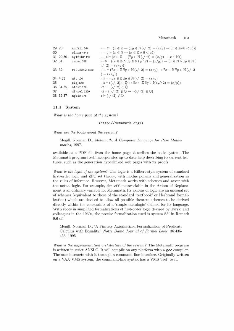
Metamath 103
29 28 anc2li 264 ······ 7 ` (x ∈ Z → (∃y ∈ N (√
‘ 2) = (x/y) → (x ∈ Z∧0 < x)))30 elnnz 4645 ······ 7 ` (x ∈ N ↔ (x ∈ Z ∧ 0 < x))31 29,30 syl6ibr 197 ····· 6 ` (x ∈ Z → (∃y ∈ N (
√‘ 2) = (x/y) → x ∈ N))
32 31 impac 318 ···· 5 ` ((x ∈ Z ∧ ∃y ∈ N (√
‘ 2) = (x/y)) → (x ∈ N ∧ ∃y ∈ N (√‘ 2) = (x/y)))
33 32 r19.22i2 1310 ··· 4 ` (∃x ∈ Z ∃y ∈ N (√
‘ 2) = (x/y) → ∃x ∈ N∃y ∈ N (√
‘ 2) = (x/y))
34 4,33 mto 100 ·· 3 ` ¬∃x ∈ Z ∃y ∈ N (√
‘ 2) = (x/y)35 elq 4705 ·· 3 ` ((
√‘ 2) ∈ Q ↔ ∃x ∈ Z ∃y ∈ N (
√‘ 2) = (x/y))
36 34,35 mtbir 178 · 2 ` ¬(√
‘ 2) ∈ Q
37 df-nel 1229 · 2 ` ((√
‘ 2) /∈ Q ↔ ¬(√
‘ 2) ∈ Q)38 36,37 mpbir 176 1 ` (
√‘ 2) /∈ Q
11.4 System
What is the home page of the system?
<http://metamath.org/>
What are the books about the system?
Megill, Norman D., Metamath, A Computer Language for Pure Mathe-matics, 1997.
available as a PDF file from the home page, describes the basic system. TheMetamath program itself incorporates up-to-date help describing its current fea-tures, such as the generation hyperlinked web pages with its proofs.
What is the logic of the system? The logic is a Hilbert-style system of standardfirst-order logic and ZFC set theory, with modus ponens and generalization asthe rules of inference. However, Metamath works with schemes and never withthe actual logic. For example, the wff metavariable in the Axiom of Replace-ment is an ordinary variable for Metamath. Its axioms of logic are an unusual setof schemes (equivalent to those of the standard ‘textbook’ or Herbrand formal-ization) which are devised to allow all possible theorem schemes to be deriveddirectly within the constraints of a ‘simple metalogic’ defined for its language.With roots in simplified formalizations of first-order logic devised by Tarski andcolleagues in the 1960s, the precise formalization used is system S3′ in Remark9.6 of:
Megill, Norman D., ‘A Finitely Axiomatized Formalization of PredicateCalculus with Equality,’ Notre Dame Journal of Formal Logic, 36:435-453, 1995.
What is the implementation architecture of the system? The Metamath programis written in strict ANSI C. It will compile on any platform with a gcc compiler.The user interacts with it through a command-line interface. Originally writtenon a VAX VMS system, the command-line syntax has a VMS ‘feel’ to it.
104 Norman Megill
What does working with the system look like? Except possibly for simple theo-rems in propositional logic, it is not a system for the casual user to build proofswith. On the one hand, its command-line interface is reasonably user-friendly,with extensive help and clear and detailed error messages. On the other hand,many small theorems or lemmas are needed to build up a framework suitable,for example, for proving the irrationality of the square root of 2. Although herethis was proved with half a dozen lemmas on top of previously proved results,over 2000 lemmas are ultimately involved in proving it all the way back to theZFC axioms. An intimate familiarity with the database is needed to build newproofs efficiently.
Once a theorem is proved, there are extensive tools for displaying and ana-lyzing its proof. For example, there is a command to trace back the axioms thatwere involved in proving a given theorem, so it is easy to determine whether saythe Axiom of Choice was used. Mechanically following any proof is trivial, sincethe metalogical rules of inference are so simple.
What is special about the system compared to other systems?
1. It is a proof verifier, not an automated prover. The proof verification is fast;the verification of the construction of real numbers (thousands of lemmas)takes a couple of seconds on a modern computer.
2. The proof verification engine makes no assumptions about the underlyinglogic; instead all axioms, including those of propositional calculus, are placedin the database. Weaker systems of logic, such as intuitionistic or quantumlogic, can be handled with different sets of axioms.
3. There is no explicit deduction theorem and it is rarely used even implicitly. Inset theory, an interesting use of the Axiom of Extensionality provides nearlythe same power, but without the exponential explosion of Hilbert-style stepsthat results from an application of the standard deduction theorem.
4. The core verification algorithm is very simple, being essentially nothing morethan substitution of expressions for variables, enhanced with checking forconflicts of variables that should be distinct.
What are other versions of the system? A demo Java applet, ‘Metamath Soli-taire,’ incorporates Metamath’s ZFC axiom system (as well as a few other sys-tems of logic). In this version, a unification algorithm lets the user know exactlywhat possibilities are available at any point in a proof, making it impossible tomake a ‘mistake.’ The applet is not practical for larger proofs.
In its present form, Metamath treats definitions as additional axioms addedto the system, and an unsound definition can result in inconsistency. Raph Levienis developing a new language called Ghilbert (ghilbert.org) that has its roots inMetamath but guarantees the soundness of definitions and provides features use-ful for collaborative work. He has written translators from Metamath to Ghilbertand vice-versa. One of his long-term goals is an HOL to Ghilbert translator.
Who are the people behind the system? Norman Megill.
Metamath 105
What are the main user communities of the system? The only users who havebuilt significant proofs are its author and Raph Levien. Several users have con-tributed shorter proofs of some propositional calculus theorems.
The ‘consumers’ of the system are the visitors to its web pages, where theproofs are displayed. The site, in existence since 1997, currently has around10000 visitors per year.
What large mathematical formalizations have been done in the system? Thelargest projects have been the construction of real and complex numbers, thedevelopment of Hilbert space from this foundation, and as a separate databasea large collection of theorems of quantum logic (orthomodular lattices).
The Hilbert space and quantum logic projects were used to verify a number ofnew results in these fields that have resulted in several papers. The papers presenttheir proofs in the traditional informal fashion; the Metamath verifications weredone simply to provide confidence that no errors were made in the proofs.
What representation of the formalization has been put in this paper? The axiomsof classical first-order logic and ZFC set theory.
What needs to be explained about this specific proof? In the source code, theuser places the assertion to be proved but omits the proof. The user builds theproof within the program in an interactive fashion, which is then written to thesource by the program. The native format of the proofs is a reverse-Polish list ofprevious assertions that are unified to construct the proof, and they can be storedor converted to that representation if desired, but they tend to be very long. Theones shown here are in a compressed format that is not human-readable but isefficient in terms of storage space.
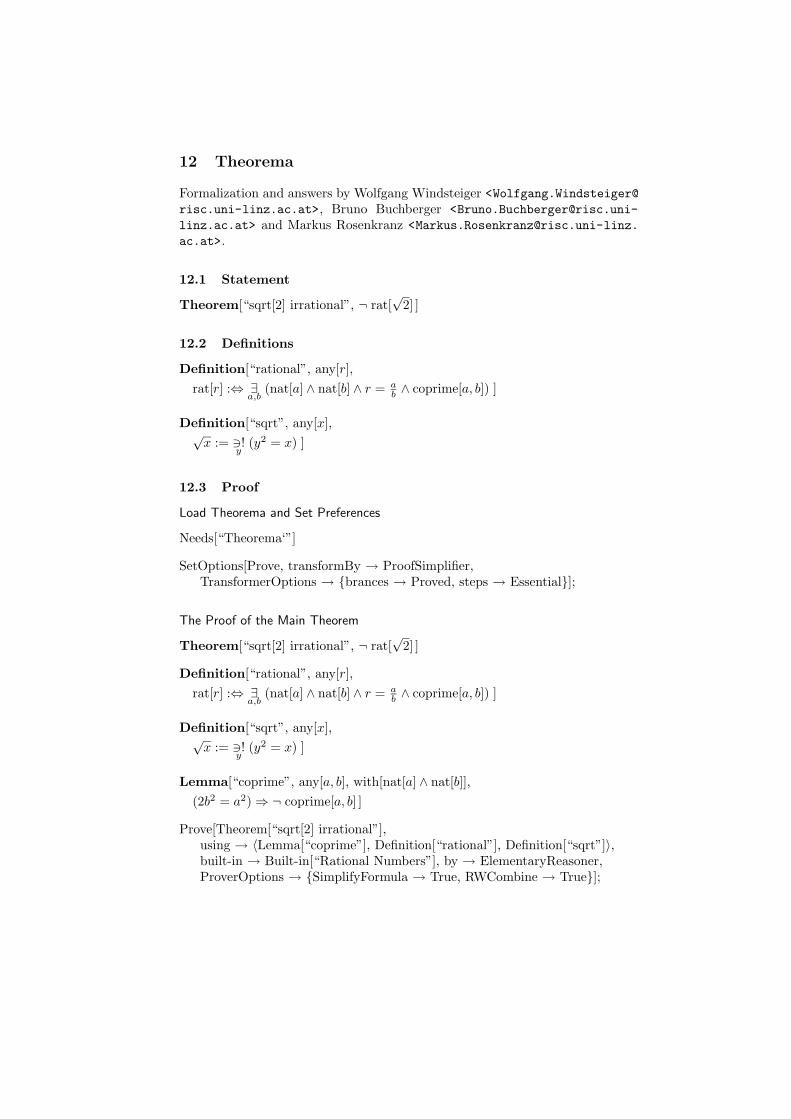
12 Theorema
Formalization and answers by Wolfgang Windsteiger <[email protected]>, Bruno Buchberger <[email protected]
linz.ac.at> and Markus Rosenkranz <[email protected].
ac.at>.
12.1 Statement
Theorem[“sqrt[2] irrational”, ¬ rat[√
2] ]
12.2 Definitions
Definition[“rational”, any[r],
rat[r] :⇔ ∃a,b
(nat[a] ∧ nat[b] ∧ r = ab∧ coprime[a, b]) ]
Definition[“sqrt”, any[x],√
x := 3!y
(y2 = x) ]
12.3 Proof
Load Theorema and Set Preferences
Needs[“Theorema‘”]
SetOptions[Prove, transformBy → ProofSimplifier,TransformerOptions → brances → Proved, steps → Essential];
The Proof of the Main Theorem
Theorem[“sqrt[2] irrational”, ¬ rat[√
2] ]
Definition[“rational”, any[r],
rat[r] :⇔ ∃a,b
(nat[a] ∧ nat[b] ∧ r = ab∧ coprime[a, b]) ]
Definition[“sqrt”, any[x],√
x := 3!y
(y2 = x) ]
Lemma[“coprime”, any[a, b], with[nat[a] ∧ nat[b]],
(2b2 = a2) ⇒ ¬ coprime[a, b] ]
Prove[Theorem[“sqrt[2] irrational”],using → 〈Lemma[“coprime”], Definition[“rational”], Definition[“sqrt”]〉,built-in → Built-in[“Rational Numbers”], by → ElementaryReasoner,ProverOptions → SimplifyFormula → True, RWCombine → True];
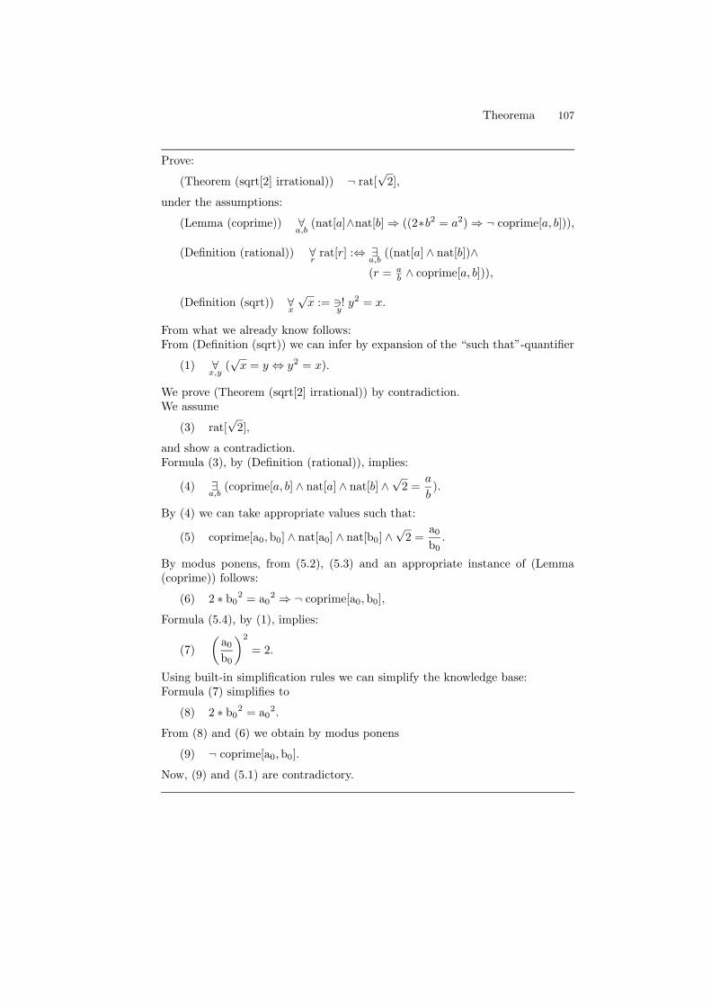
Theorema 107
Prove:
(Theorem (sqrt[2] irrational)) ¬ rat[√
2],
under the assumptions:
(Lemma (coprime)) ∀a,b
(nat[a]∧nat[b] ⇒ ((2∗b2 = a2) ⇒ ¬ coprime[a, b])),
(Definition (rational)) ∀r
rat[r] :⇔ ∃a,b
((nat[a] ∧ nat[b])∧(r = a
b∧ coprime[a, b])),
(Definition (sqrt)) ∀x
√x := 3!
yy2 = x.
From what we already know follows:From (Definition (sqrt)) we can infer by expansion of the “such that”-quantifier
(1) ∀x,y
(√
x = y ⇔ y2 = x).
We prove (Theorem (sqrt[2] irrational)) by contradiction.We assume
(3) rat[√
2],
and show a contradiction.Formula (3), by (Definition (rational)), implies:
(4) ∃a,b
(coprime[a, b] ∧ nat[a] ∧ nat[b] ∧√
2 =a
b).
By (4) we can take appropriate values such that:
(5) coprime[a0,b0] ∧ nat[a0] ∧ nat[b0] ∧√
2 =a0
b0.
By modus ponens, from (5.2), (5.3) and an appropriate instance of (Lemma(coprime)) follows:
(6) 2 ∗ b02 = a0
2 ⇒ ¬ coprime[a0,b0],
Formula (5.4), by (1), implies:
(7)
(
a0
b0
)2
= 2.
Using built-in simplification rules we can simplify the knowledge base:Formula (7) simplifies to
(8) 2 ∗ b02 = a0
2.
From (8) and (6) we obtain by modus ponens
(9) ¬ coprime[a0,b0].
Now, (9) and (5.1) are contradictory.
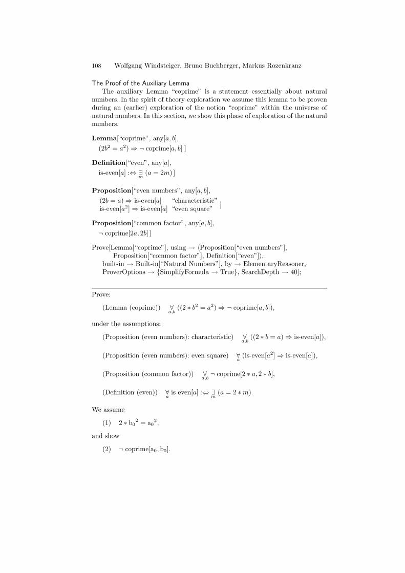
108 Wolfgang Windsteiger, Bruno Buchberger, Markus Rozenkranz
The Proof of the Auxiliary Lemma
The auxiliary Lemma “coprime” is a statement essentially about naturalnumbers. In the spirit of theory exploration we assume this lemma to be provenduring an (earlier) exploration of the notion “coprime” within the universe ofnatural numbers. In this section, we show this phase of exploration of the naturalnumbers.
Lemma[“coprime”, any[a, b],
(2b2 = a2) ⇒ ¬ coprime[a, b] ]
Definition[“even”, any[a],
is-even[a] :⇔ ∃m
(a = 2m) ]
Proposition[“even numbers”, any[a, b],
(2b = a) ⇒ is-even[a] “characteristic”is-even[a2] ⇒ is-even[a] “even square”
]
Proposition[“common factor”, any[a, b],
¬ coprime[2a, 2b] ]
Prove[Lemma[“coprime”], using → 〈Proposition[“even numbers”],Proposition[“common factor”], Definition[“even”]〉,
built-in → Built-in[“Natural Numbers”], by → ElementaryReasoner,ProverOptions → SimplifyFormula → True, SearchDepth → 40];
Prove:
(Lemma (coprime)) ∀a,b
((2 ∗ b2 = a2) ⇒ ¬ coprime[a, b]),
under the assumptions:
(Proposition (even numbers): characteristic) ∀a,b
((2 ∗ b = a) ⇒ is-even[a]),
(Proposition (even numbers): even square) ∀a
(is-even[a2] ⇒ is-even[a]),
(Proposition (common factor)) ∀a,b
¬ coprime[2 ∗ a, 2 ∗ b],
(Definition (even)) ∀a
is-even[a] :⇔ ∃m
(a = 2 ∗ m).
We assume
(1) 2 ∗ b02 = a0
2,
and show
(2) ¬ coprime[a0,b0].
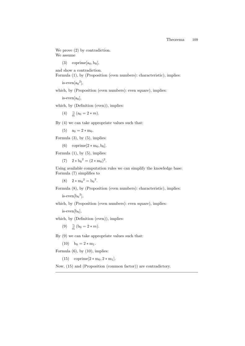
Theorema 109
We prove (2) by contradiction.We assume
(3) coprime[a0,b0],
and show a contradiction.Formula (1), by (Proposition (even numbers): characteristic), implies:
is-even[a02],
which, by (Proposition (even numbers): even square), implies:
is-even[a0],
which, by (Definition (even)), implies:
(4) ∃m
(a0 = 2 ∗ m).
By (4) we can take appropriate values such that:
(5) a0 = 2 ∗ m0.
Formula (3), by (5), implies:
(6) coprime[2 ∗ m0,b0].
Formula (1), by (5), implies:
(7) 2 ∗ b02 = (2 ∗ m0)
2.
Using available computation rules we can simplify the knowledge base:Formula (7) simplifies to
(8) 2 ∗ m02 = b0
2.
Formula (8), by (Proposition (even numbers): characteristic), implies:
is-even[b02],
which, by (Proposition (even numbers): even square), implies:
is-even[b0],
which, by (Definition (even)), implies:
(9) ∃m
(b0 = 2 ∗ m).
By (9) we can take appropriate values such that:
(10) b0 = 2 ∗ m1.
Formula (6), by (10), implies:
(15) coprime[2 ∗ m0, 2 ∗ m1].
Now, (15) and (Proposition (common factor)) are contradictory.
110 Wolfgang Windsteiger, Bruno Buchberger, Markus Rozenkranz
12.4 System
What is the home page of the system?
<http://www.theorema.org/>
What are the books about the system? The essential theoretical ideas involved inthe Theorema system can be found already in [5]. A comprehensive descriptionof the basic design of a computer-system based on these ideas is then given in[1]. For a more elaborate exposition and for concrete design principles of thecurrent Theorema system, we refer to the survey papers [[3,4]].
Most of the system components are described in all detail in journal papers,conference proceedings articles, or technical reports. All downloadable materialcan be found on the Theorema homepage.
What is the logic of the system? The logic frame of Theorema is higher orderpredicate logic, which is extended by the language construct “sequence vari-ables”. Sequence variables are variables for which an arbitrary finite number ofterms can be substituted. Sequence variables are a convenient construct for theformulation of algorithms in terms of pattern matching within logic. Thus, theTheorema language is also particularly suited for expressing logic algorithms liketheorem provers etc. A logical study of sequence variables is given in [6].
In fact, the Theorema system is a (growing) collection of various generalpurpose and special theorem provers. The general purpose provers (like the firstorder predicate logic natural deduction prover) are valid only for special frag-ments of predicate logic (e.g. first order predicate logic). The special proversare valid only under the additional assumption that special knowledge is avail-able that characterizes the underlying special theory. For example, the (variousversions) of the induction prover assume that, for certain functions, an induc-tion principle holds; the geometry prover based on the Grobner bases methodassumes that the universe of discourse is the field of complex numbers and thebasic properties of complex numbers are available; the set theory prover assumesthat the axioms and basic properties of set theory are valid. We do not yet havea prover for a general version of higher order logic. Of course, this approachto building a theorem proving system supposes that the correctness of specialtheorem provers is (automatically) proved w.r.t. to more general provers. So far,this research program is only partially carried out. For example, Grobner basestheory is proved correct in a fairly formal way. A complete formal proof withinTheorema is planned for the near future.
What is the implementation architecture of the system? All Theorema ‘reason-ers’ (provers, solvers, and simplifiers) are written in the programming languageof Mathematica. Theorema does not use the Mathematica algorithm library orany implicit mathematical knowledge presupposed in Mathematica algorithms.The Theorema language is a version of higher order predicate logic. The cur-rently available reasoners comprise general purpose reasoners (several methodsfor proving in first order predicate logic, a prover for equational reasoning, or
Theorema 111
a general simplification prover based on equality rewriting) and special purposereasoners (like Collins’ decision procedure for the theory of real closed fields, aspecial prover for geometry based on algebraic techniques like Grobner bases, orthe simplification prover for number domains used in the proofs shown in Sec-tion 12.3) that are valid only in particular theories. Various external provers likee.g. Otter can be accessed through Theorema by translating Theorema formulaeto the specific input format for these provers and getting the results back. Rea-soners available in Mathematica can also be accessed by Theorema upon explicitrequest by the user. The Theorema language includes a programming languageas a natural sub-language.
Theorema provers have a modular structure, i.e. every Theorema prover iscomposed from smaller units, so-called ‘special prover modules’. These provermodules are separate units, and can therefore be combined in arbitrary way. Inthe current status, the access to special prover modules is restricted to the sys-tem developers, but a mechanism for users to compose their own provers fromavailable special prover modules is planned for future versions of the system.Theorema uses a general proof search procedure that maintains a global proofobject. The proof object has a tree-structure where each node in the tree rep-resents a proof situation made up basically from the proof goal and the currentassumptions. In each step, the proof search procedure tries to apply a specialprover module in order to simplify the current proof situation. A special provermodule can be applied to a proof situation if one of its inference rules can beapplied to the proof situation. Inference rules in the prover modules are im-plemented as Mathematica programs that take a proof situation as parameterand return a new proof situation. Applicability of an inference rule is tested bypattern matching on the parameters of the Mathematica program against thecurrent proof situation. When applying a special prover module to a proof situa-tion the proof search procedure inserts the result of the first applicable rule as anew node into the global proof object. The proof search continues until a trivialproof situation (e.g. the goal is identical to one of the assumptions) appears onone branch of the tree, in which case the proof succeeds, or until the maximalsearch depth is exceeded on all branches, in which case the proof attempt fails.
What does working with the system look like? The current version of Theoremais implemented as an extension package to Mathematica, thus, the standardway of working with Theorema is an interactive user-system-dialog in the well-known Mathematica notebook FrontEnd. The Mathematica notebook FrontEndsupports configurable two-dimensional mathematical notation both in input andoutput. The examples in Section 12.3 demonstrate a typical Theorema session.Two categories of commands are available for the user:
Organization of Knowledge: The Theorema Formal Text Language allowsthe user to enter arbitrary definitions, axioms, propositions, algorithms, etc.to the system and combine such formulae into theories in a nested way sothat hierarchies of mathematical knowledge bases (theories) can be built up.All formulae may receive key words and labels for easy reference. Labels,
112 Wolfgang Windsteiger, Bruno Buchberger, Markus Rozenkranz
however, carry no logical meaning. Declaration of free variables and condi-tions on these variables are specified using the keywords ‘any’ and ‘with’.The individual formulae can be entered in a two-dimensional syntax veryclose to how formulae are written in mathematical textbooks. The actualinput of arbitrary two-dimensional notation and special mathematical sym-bols is supported by the standard Mathematica notebook FrontEnd throughinput palettes and keyboard shortcuts. The input of Theorema-specific no-tation, like e.g. a formal text entity containing labelled formulae as used inProposition “even numbers”, is taken care of by additional input palettes.The definitions, theorems, lemmata, and propositions as they display in Sec-tion 12.3 illustrate some of the features of the Formal Text Language.Note that the Theorema language also supports several notational variantsfor mathematical syntax in order to accommodate to the preferences of theuser. As an example, we used the standard form of the existential quantifier
∃a,b
(nat[a] ∧ nat[b] ∧ r =a
b∧ coprime[a, b])
in Definition “rational” as given in Section 12.2. Supported notational vari-ants, which would all be interpreted by all Theorema provers in exactly thesame way, are:
∃nat[a],nat[b]
(r =a
b∧ coprime[a, b]),
∃nat[a,b]
(r =a
b∧ coprime[a, b]), or
∃a,b
nat[a]∧nat[b](r =
a
b∧ coprime[a, b]).
Mathematical Activities: Mathematical knowledge can then be processedin various ways using the Theorema User Language. Currently, the UserLanguage supports ‘proving’, ‘solving’, and ‘simplifying’, see the commandsProve[...] in Section 12.3 for typical examples. These examples also ex-hibit, how knowledge specified in the Formal Text Language can be referredto in the User Language. Note also, that the keywords such as ‘any’ or ‘with’are processed when formulae are passed to a prover: Compare the formulaeas they are echoed at the beginning of the proof to how they appear in theFormal Text Language.Proofs (or traces of solving or simplifying) are generated completely auto-matically and display very much in the form as they would be written inmathematical textbooks including intermediate explanatory text in naturallanguage. Alternatively, Theorema also offers an interactive mode, whereuser-interaction during proof generation is supported. Mathematical formu-lae are displayed in two-dimensional syntax. The proofs appear in the The-orema system almost exactly as they are typeset in Section 12.3.However, some of the features of the Theorema user interface cannot bemodelled in the style of this paper:
Theorema 113
– Proof branches are organized in hierarchically nested cells, which can beopened or closed by double-clicking the cell bracket on the right marginof the window. This allows the user to hide (or display) certain parts ofa proof easily by mouse-click.
– Formula labels are active elements, such that clicking a formula referencein the running text shows the full formula in a separate pop-up window.
– Goal formulae, assumptions, labels, and explanatory text use differentcolors.
Also, there are means in Theorema to design and implement one’s own syntaxincluding the design of new mathematical symbols of arbitrary complexity(‘logicographic symbols’).
What is special about the system compared to other systems?
– Theorema is both a logic language and a programming language. This meansthat, for example, within the same language and system, a formula thatdescribes an algorithm can be proved correct and can then be executed onconcrete input.
– The three fundamental mathematical activities proving, solving, and simpli-fying can be done in one uniform language and logic frame.
– Theorema is a multi-method system: instead of using one uniform proofmethod for all of mathematics Theorema provides sophisticated special prov-ers for certain mathematical theories. These special provers are partly basedon powerful computer algebra methods, which were the research focus of theworking group in earlier years.
– Theorema has an attractive two-dimensional, extensible syntax.– Most of the Theorema provers generate proofs in a natural, human-readable
style with intermediate explanatory text and various tools that help to getvarious (contracted and expanded) views of proofs.
– Theorema has various structuring mechanisms for large mathematical knowl-edge bases, notably the recursive ‘Theory’ construct and a functor construct,which is similar to but more general than the functor construct of SML.
What are other versions of the system? There are no other versions of the system.The current version is free for download from the Theorema webpage under“software”.
Who are the people behind the system? The development of Theorema has beeninitiated by Bruno Buchberger, who also implemented first prototypes in the mid1990’s and directs the project since then in cooperation with Tudor Jebelean andWolfgang Windsteiger. Current senior Theorema researchers are, in addition,Temur Kutsia, Florina Piroi, and Markus Rosenkranz. Former Theorema PhDstudents, who contributed to the system, are Daniela Vasaru-Dupre, MirceaMarin, Koji Nakagawa, Judit Robu, and Elena Tomuta. For a complete (andalways up-to-date) listing of persons involved in the Theorema project we referto the Theorema webpage.
114 Wolfgang Windsteiger, Bruno Buchberger, Markus Rozenkranz
What are the main user communities of the system? There is a small communityof alpha testers, mainly math researchers and math teachers. A major didacticcase study in undergraduate math education at the Johannes Kepler Universityof Linz and the Polytechnic University Hagenberg is under way.
What large mathematical formalizations have been done in the system? Elemen-tary analysis (with the typical epsilon/delta proofs), equivalence relations andpartitions based on set theory, polynomial interpolation, the theory of lists withverified list algorithms like sorting, and the automated synthesis of the Grobnerbases algorithm.
What representation of the formalization has been put in this paper? The for-malization in Section 12.3 should be self-explanatory. In fact, it is a main designprinciple of Theorema that formalizations using the Theorema language con-structs should be self-explanatory and easy to read. The theorem is formulatedas a statement over the positive real numbers. The first part shown in Sec-tion 12.3 contains the main proof that reduces the problem over the positivereals to a lemma over the natural numbers. Section 12.3 shows the second partthat contains the proof of the auxiliary lemma over the naturals.
What needs to be explained about this specific proof? In the proof of the maintheorem, we assume that all variables range over the positive real numbers, i.e. allformulae in the knowledge base should be true statements in the domain ofpositive real numbers.
The proof of the theorem as shown in Section 12.3 is generated completelyautomatically within Theorema. The only user-interactions required are
– to choose an appropriate prover from the Theorema prover library (in theexample the “Elementary Reasoner”),
– to specify appropriate prover options for the chosen prover, and– to provide the auxiliary Lemma “coprime” necessary in the proof.
In the spirit of the layered approach of Theorema, the auxiliary lemma can thenbe proved in a separate proving session as shown in Section 12.3. Again, auxiliaryknowledge needed in this proof (in the example the Propositions “even numbers”and “common factor”) can be proved in separate phases of exploring a theory.However, we do not present the proofs of these propositions here, because wheninvestigating the irrationality of
√2 one would usually consider these proposi-
tions to be known properties of natural numbers. Phases of theory explorationcan be structured bottom-up or top-down just like human mathematicians buildup hierarchically structured mathematical knowledge.
Typically, different phases of theory exploration are characterized by usingdifferent proving techniques. In the case of automated theory exploration usingTheorema this means that switching from one exploration phase to anotherwould be reflected in changing the prover that is used in the Prove-calls. In thisexample, in fact, we use the Elementary Reasoner in both phases, but we allow
Theorema 115
the prover to access different portions of built-in computational knowledge ineither phase.
The special feature of the Elementary Reasoner used for generating the proofsshown in Section 12.3 is the smooth integration of ‘proving’ and ‘simplifying’(‘computing’) within one system. ‘Simplifying’, here, means ‘simplifying expres-sions (to canonical form) based on the algorithmic semantics of the language’.The algorithmic semantics of the Theorema language consists of computationrules for the algorithmic part of the language8, i.e. finite sets, finite tuples,quantifiers with a finite range, and basic arithmetic on numbers. Sets, tuples,and quantifiers are represented as special data structures and the operations onthese entities are implemented in the Theorema language semantics using theprogramming language of Mathematica. Only for arithmetic on natural num-bers, integers, and rational numbers the Theorema semantics may access thearithmetic rules from the underlying Mathematica system.
In the example, the option built-in→Built-in["Rational Numbers"] al-lows the Elementary Reasoner explicitly to use built-in computation rules foroperations on rational numbers. Arithmetic on numbers is, in fact, the onlycase, where Theorema silently relies on the mathematical algorithm library avail-able from Mathematica9. On explicit user request, however, the interface allowsthis prover to even access special simplification algorithms from Mathemat-ica when performing computational simplification. Specifying the prover optionSimplifyFormula→True (default value is False) tells the prover to post-processany formula obtained from a computation by Mathematica’s FullSimplify func-tion. FullSimplify is a black-box simplifier for Mathematica expressions, whichuses powerful simplification rules, in particular for arithmetic expressions. More-over, the prover performs additional simplification of equalities involving arith-metic expressions, such that certain equalities are turned into equalities thatare more likely to be usable for rewriting. In our context, the correctness ofthe built-in simplifier is based exclusively on the field axioms (for proofs overthe reals) and the ring axioms (for proofs over the naturals10), respectively. Inother words, the ‘hidden knowledge’ used by the simplifier are only the field orring axioms10, respectively. All other knowledge, e.g. Lemma “coprime”, Propo-sition “even numbers”, and Proposition “common factor”, must be mentionedexplicitly in the call of the prover.
A combination of these capabilities is used in the main proof when simplifyingformula
(7)
(
a0
b0
)2
= 2
to
8 In contrast, the semantics of the non-algorithmic part of the language is coded intoinference rules that make up the Theorema special prover modules.
9 Apart from that, Mathematica is used just as a programming environment!10 To be precise: the simplifier for the naturals uses the ring axioms without the axiom
ensuring the existence of additive inverses.
116 Wolfgang Windsteiger, Bruno Buchberger, Markus Rozenkranz
(8) 2b02 = a0
2
and in the proof of the auxiliary lemma when simplifying
(7) 2b02 = (2m0)
2
to
(8) 2m02 = b0
2.
Definition “sqrt” uses a convenient language construct available in Theorema:The ‘the-unique’-quantifier 3!
yPy denotes ‘the unique y satisfying Py’. The ex-
pression f [x] := 3!y
Px,y is a means to express an implicit definition for the
function f , for which, of course, we need to verify ∀x∃!y
Px,y beforehand. In the
concrete example of Definition “sqrt”, we assume that ∀x∃!y
y2 = x holds over the
positive real numbers. Based on this convention the prover applies an inferencerule for the ‘the-unique’-quantifier in order to rewrite Definition “sqrt” in themain proof into
(2) ∀x,y
(√
x = y ⇔ y2 = x).
All other steps in the proofs are basic predicate logic and therefore require nofurther explanation.
References
1. B. Buchberger. Symbolic Computation: Computer Algebra and Logic. In K. Schulz,editor, FroCoS: Frontiers of Combined Systems, 1996.
2. B. Buchberger. Algorithm Supported Mathematical Theory Exploration. In B.Buchberger and John Campbell, editors, Proceedings of AISC 2004 (7th Inter-national Conference on Artificial Intelligence and Symbolic Computation, volume3249 of Springer Lecture Notes in Artificial Intelligence, RISC, Johannes KeplerUniversity, Austria, September 22-24 2004. Springer Berlin Heidelberg. ISSN 0302-9743, ISBN 3-540-23212-5.
3. B. Buchberger, C. Dupre, T. Jebelean, F. Kriftner, K. Nakagawa, D. Vasaru, andW. Windsteiger. The Theorema Project: A Progress Report. In M. Kerber andM. Kohlhase, editors, Symbolic Computation and Automated Reasoning (Proceed-ings of CALCULEMUS 2000, Symposium on the Integration of Symbolic Computa-tion and Mechanized Reasoning), pages 98–113. St. Andrews, Scotland, Copyright:A.K. Peters, Natick, Massachusetts, 6-7 August 2000.
4. B. Buchberger, T. Jebelean, F. Kriftner, M. Marin, E. Tomuta, and D. Vasaru. ASurvey of the Theorema project. In W. Kuechlin, editor, Proceedings of ISSAC’97(International Symposium on Symbolic and Algebraic Computation, Maui, Hawaii,July 21-23, 1997), ACM Press 1997, pages 384–391, 1997.
5. B. Buchberger and F. Lichtenberger. Mathematik fur Informatiker I. SpringerVerlag, 2nd edition, 1981.
Theorema 117
6. T. Kutsia and B. Buchberger. Predicate Logic with Sequence Variables and Se-quence Function Symbols. In Andrea Asperti, Grzegorz Bancerek, and AndrzejTrybulec, editors, Proceedings of the 3rd International Conference on Mathemati-cal Knowledge Management, MKM’04, volume 3119 of Lecture Notes in ComputerScience, pages 205–219, Bialowieza, Poland, Sep 19–21 2004. Springer Verlag.
13 Lego
Formalization by Conor McBride <[email protected]>. Answers by ConorMcBride and Robert Pollack <[email protected]>.
13.1 Statement
b|nata|nat(Eq (times two (times a a)) (times b b))->
(Eq a zero /\ Eq b zero)
13.2 Definitions
Definition of Prime
[Prime = [p:nat]
a|NATb,x|NatPhi|Prop
q:Eq (times p x) (times a b)
phiL:a’:nat
(Eq a (times p a’))->(Eq x (times a’ b))->Phi
phiR:b’:nat
(Eq b (times p b’))->(Eq x (times a b’))->Phi
Phi
];
13.3 Proof
Conor’s proof that 2 has no rational root.
This proof is accepted by LEGO version 1.3.1 with its standard library.
Make lib_nat; (* loading basic logic, nat, plus, times etc *)
(* note, plus and times are defined by recursion on their first arg *)
Alternative eliminators for nat
LEGO’s induction tactic figures out which induction principle to use by lookingat the type of the variable on which we’re doing induction. Consequently, we canpersuade the tactic to use an alternative induction principle if we alias the type.
Nat_elim is just the case analysis principle for natural numbers—the sameas the induction principle except that there’s no inductive hypothesis in the stepcase. It’s intended to be used in combination with. . .
. . . NAT_elim, which performs no case analysis but says you can have aninductive hypothesis for any smaller value, where y is smaller than suc (plus
x y). This is ‘well-founded induction’ for the < relation, but expressed moreconcretely.
The effect is very similar to that of ‘Case’ and ‘Fix’ in Coq.
Lego 119
[Nat = nat];
[NAT = Nat];
(* case analysis: just a weakening of induction *)
Goal Nat_elim : Phi:nat->Type
phiz:Phi zero
phis:n:NatPhi (suc n)
n:NatPhi n;
intros ___;
Expand Nat; Induction n;
Immed;
intros; Immed;
Save;
(* suc-plus guarded induction: the usual proof *)
Goal NAT_elim :
Phi:nat->Type
phi:n:Nat
ih:x,y|Nat(Eq n (suc (plus x y)))->Phi y
Phi n
n:NATPhi n;
intros Phi phi n’;
(* claim that we can build the hypothesis collector for each n *)
Claim n:natx,y|Nat(Eq n (suc (plus x y)))->Phi y;
(* use phi on the claimed collector *)
Refine phi n’ (?+1 n’);
(* now build the collector by one-step induction *)
Induction n;
Qnify; (* nothing to collect for zero *)
intros n nhyp;
Induction x; (* case analysis on the slack *)
Qnify;
Refine phi; (* if the bound is tight, use phi to *)
Immed; (* generate the new member of the collection *)
Qnify;
Refine nhyp; (* otherwise, we’ve already collected it *)
Immed;
Save;
Equational laws governing plus and times: some of these are doubtless in thelibrary, but it takes longer to remember their names than to prove them again.
Goal plusZero : x:natEq (plus x zero) x;
Induction x;
Refine Eq_refl;
intros;
Refine Eq_resp suc;
Immed;
Save;
120 Conor McBride
Goal plusSuc : x,y:natEq (plus x (suc y)) (suc (plus x y));
Induction x;
intros; Refine Eq_refl;
intros;
Refine Eq_resp suc;
Immed;
Save;
Goal plusAssoc : x,y,z:natEq (plus (plus x y) z) (plus x (plus y z));
Induction x;
intros; Refine Eq_refl;
intros;
Refine Eq_resp suc;
Immed;
Save;
Goal plusComm : x,y:natEq (plus x y) (plus y x);
Induction y;
Refine plusZero;
intros y yh x;
Refine Eq_trans (plusSuc x y);
Refine Eq_resp suc;
Immed;
Save;
Goal plusCommA : x,y,z:natEq (plus x (plus y z)) (plus y (plus x z));
intros;
Refine Eq_trans ? (plusAssoc ???);
Refine Eq_trans (Eq_sym (plusAssoc ???));
Refine Eq_resp ([w:nat]plus w z);
Refine plusComm;
Save;
Goal timesZero : x:natEq (times x zero) zero;
Induction x;
Refine Eq_refl;
intros;
Immed;
Save;
Goal timesSuc : x,y:natEq (times x (suc y)) (plus x (times x y));
Induction x;
intros; Refine Eq_refl;
intros x xh y;
Equiv Eq (suc (plus y (times x (suc y)))) ?;
Equiv Eq ? (suc (plus x (plus y (times x y))));
Refine Eq_resp;
Qrepl xh y;
Refine plusCommA;
Save;
Goal timesComm : x,y:natEq (times x y) (times y x);
Induction y;
Lego 121
Refine timesZero;
intros y yh x;
Refine Eq_trans (timesSuc ??);
Refine Eq_resp (plus x);
Immed;
Save;
Goal timesDistL : x,y,z:natEq (times (plus x y) z)
(plus (times x z) (times y z));
Induction x;
intros; Refine Eq_refl;
intros x xh y z;
Refine Eq_trans (Eq_resp (plus z) (xh y z));
Refine Eq_sym (plusAssoc ???);
Save;
Goal timesAssoc : x,y,z:natEq (times (times x y) z) (times x (times y z));
Induction x;
intros; Refine Eq_refl;
intros x xh y z;
Refine Eq_trans (timesDistL ???);
Refine Eq_resp (plus (times y z));
Immed;
Save;
Inversion principles for equations governing plus and times: these aren’t in thelibrary, at least not in this form.
[Phi|Type]; (* Inversion principles are polymorphic in any goal *)
Goal plusCancelL : y,z|natphi:q’:Eq y zPhix|nat
q:Eq (plus x y) (plus x z)Phi;
intros ___;
Induction x;
intros;
Refine phi q;
intros x xh; Qnify;
Refine xh;
Immed;
Save;
Goal timesToZero : a,b|Nat
phiL:(Eq a zero)->Phi
phiR:(Eq b zero)->Phi
tz:Eq (times a b) zero
Phi;
Induction a;
intros; Refine phiL (Eq_refl ?);
intros a;
Induction b;
intros; Refine phiR (Eq_refl ?);
Qnify;
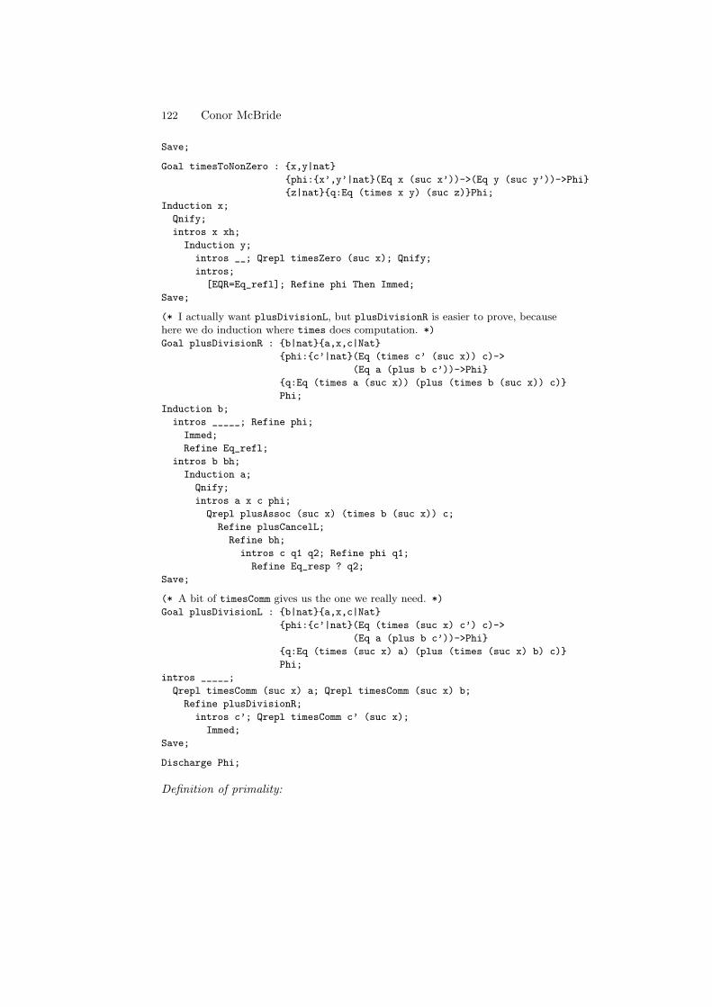
122 Conor McBride
Save;
Goal timesToNonZero : x,y|nat
phi:x’,y’|nat(Eq x (suc x’))->(Eq y (suc y’))->Phi
z|natq:Eq (times x y) (suc z)Phi;
Induction x;
Qnify;
intros x xh;
Induction y;
intros __; Qrepl timesZero (suc x); Qnify;
intros;
[EQR=Eq_refl]; Refine phi Then Immed;
Save;
(* I actually want plusDivisionL, but plusDivisionR is easier to prove, becausehere we do induction where times does computation. *)
Goal plusDivisionR : b|nata,x,c|Nat
phi:c’|nat(Eq (times c’ (suc x)) c)->
(Eq a (plus b c’))->Phi
q:Eq (times a (suc x)) (plus (times b (suc x)) c)
Phi;
Induction b;
intros _____; Refine phi;
Immed;
Refine Eq_refl;
intros b bh;
Induction a;
Qnify;
intros a x c phi;
Qrepl plusAssoc (suc x) (times b (suc x)) c;
Refine plusCancelL;
Refine bh;
intros c q1 q2; Refine phi q1;
Refine Eq_resp ? q2;
Save;
(* A bit of timesComm gives us the one we really need. *)
Goal plusDivisionL : b|nata,x,c|Nat
phi:c’|nat(Eq (times (suc x) c’) c)->
(Eq a (plus b c’))->Phi
q:Eq (times (suc x) a) (plus (times (suc x) b) c)
Phi;
intros _____;
Qrepl timesComm (suc x) a; Qrepl timesComm (suc x) b;
Refine plusDivisionR;
intros c’; Qrepl timesComm c’ (suc x);
Immed;
Save;
Discharge Phi;
Definition of primality:
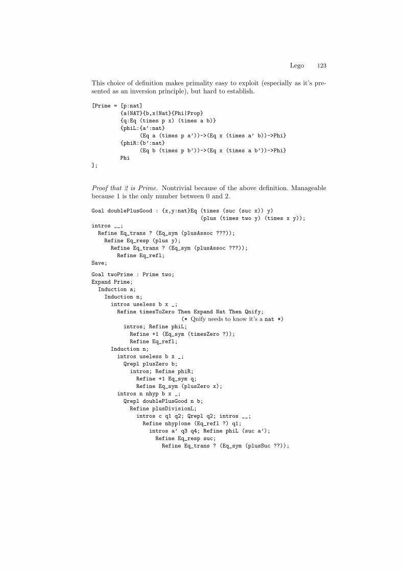
Lego 123
This choice of definition makes primality easy to exploit (especially as it’s pre-sented as an inversion principle), but hard to establish.
[Prime = [p:nat]
a|NATb,x|NatPhi|Prop
q:Eq (times p x) (times a b)
phiL:a’:nat
(Eq a (times p a’))->(Eq x (times a’ b))->Phi
phiR:b’:nat
(Eq b (times p b’))->(Eq x (times a b’))->Phi
Phi
];
Proof that 2 is Prime. Nontrivial because of the above definition. Manageablebecause 1 is the only number between 0 and 2.
Goal doublePlusGood : x,y:natEq (times (suc (suc x)) y)
(plus (times two y) (times x y));
intros __;
Refine Eq_trans ? (Eq_sym (plusAssoc ???));
Refine Eq_resp (plus y);
Refine Eq_trans ? (Eq_sym (plusAssoc ???));
Refine Eq_refl;
Save;
Goal twoPrime : Prime two;
Expand Prime;
Induction a;
Induction n;
intros useless b x _;
Refine timesToZero Then Expand Nat Then Qnify;
(* Qnify needs to know it’s a nat *)
intros; Refine phiL;
Refine +1 (Eq_sym (timesZero ?));
Refine Eq_refl;
Induction n;
intros useless b x _;
Qrepl plusZero b;
intros; Refine phiR;
Refine +1 Eq_sym q;
Refine Eq_sym (plusZero x);
intros n nhyp b x _;
Qrepl doublePlusGood n b;
Refine plusDivisionL;
intros c q1 q2; Qrepl q2; intros __;
Refine nhyp|one (Eq_refl ?) q1;
intros a’ q3 q4; Refine phiL (suc a’);
Refine Eq_resp suc;
Refine Eq_trans ? (Eq_sym (plusSuc ??));
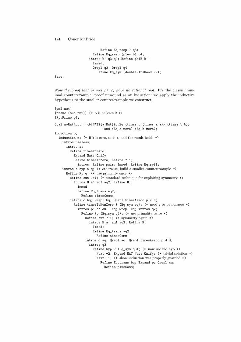
124 Conor McBride
Refine Eq_resp ? q3;
Refine Eq_resp (plus b) q4;
intros b’ q3 q4; Refine phiR b’;
Immed;
Qrepl q3; Qrepl q4;
Refine Eq_sym (doublePlusGood ??);
Save;
Now the proof that primes (≥ 2) have no rational root. It’s the classic ‘min-imal counterexample’ proof unwound as an induction: we apply the inductivehypothesis to the smaller counterexample we construct.
[pm2:nat]
[p=suc (suc pm2)] (* p is at least 2 *)
[Pp:Prime p];
Goal noRatRoot : b|NATa|Natq:Eq (times p (times a a)) (times b b)
and (Eq a zero) (Eq b zero);
Induction b;
Induction n; (* if b is zero, so is a, and the result holds *)
intros useless;
intros a;
Refine timesToZero;
Expand Nat; Qnify;
Refine timesToZero; Refine ?+1;
intros; Refine pair; Immed; Refine Eq_refl;
intros b hyp a q; (* otherwise, build a smaller counterexample *)
Refine Pp q; (* use primality once *)
Refine cut ?+1; (* standard technique for exploiting symmetry *)
intros H a’ aq1 aq2; Refine H;
Immed;
Refine Eq_trans aq2;
Refine timesComm;
intros c bq; Qrepl bq; Qrepl timesAssoc p c c;
Refine timesToNonZero ? (Eq_sym bq); (* need c to be nonzero *)
intros p’ c’ dull cq; Qrepl cq; intros q2;
Refine Pp (Eq_sym q2); (* use primality twice *)
Refine cut ?+1; (* symmetry again *)
intros H a’ aq1 aq2; Refine H;
Immed;
Refine Eq_trans aq2;
Refine timesComm;
intros d aq; Qrepl aq; Qrepl timesAssoc p d d;
intros q3;
Refine hyp ? (Eq_sym q3); (* now use ind hyp *)
Next +2; Expand NAT Nat; Qnify; (* trivial solution *)
Next +1; (* show induction was properly guarded *)
Refine Eq_trans bq; Expand p; Qrepl cq;
Refine plusComm;
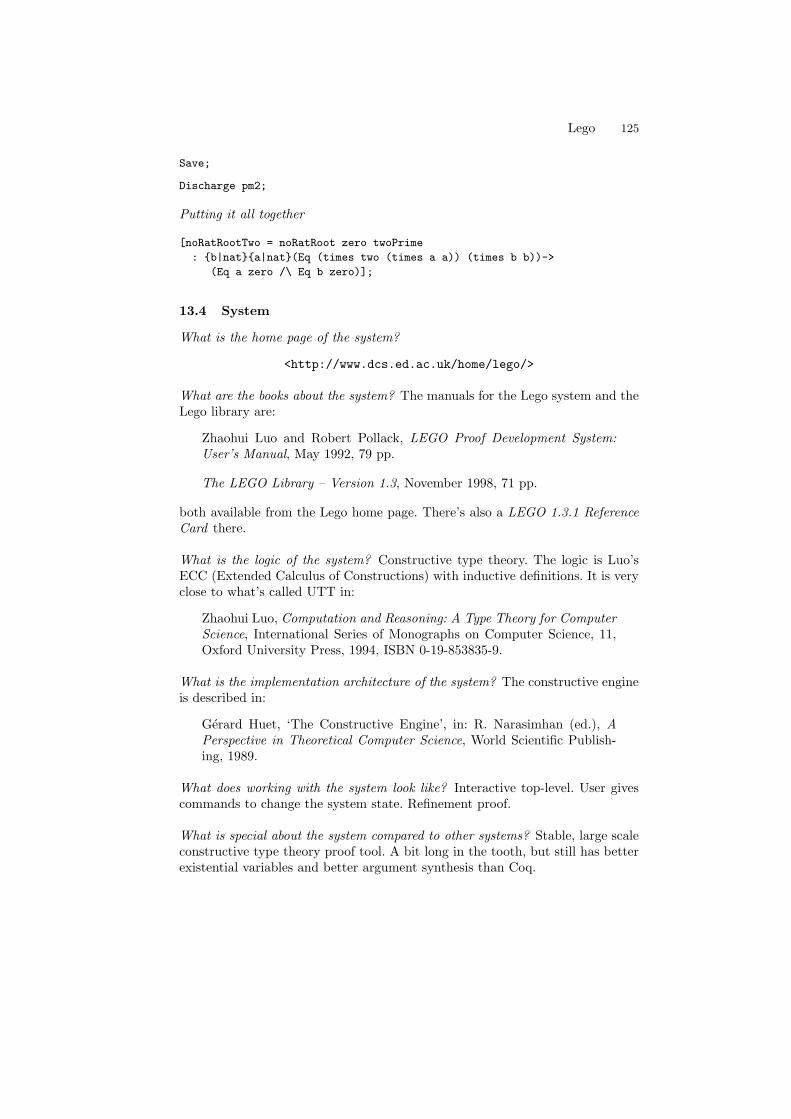
Lego 125
Save;
Discharge pm2;
Putting it all together
[noRatRootTwo = noRatRoot zero twoPrime
: b|nata|nat(Eq (times two (times a a)) (times b b))->
(Eq a zero /\ Eq b zero)];
13.4 System
What is the home page of the system?
<http://www.dcs.ed.ac.uk/home/lego/>
What are the books about the system? The manuals for the Lego system and theLego library are:
Zhaohui Luo and Robert Pollack, LEGO Proof Development System:User’s Manual, May 1992, 79 pp.
The LEGO Library – Version 1.3, November 1998, 71 pp.
both available from the Lego home page. There’s also a LEGO 1.3.1 ReferenceCard there.
What is the logic of the system? Constructive type theory. The logic is Luo’sECC (Extended Calculus of Constructions) with inductive definitions. It is veryclose to what’s called UTT in:
Zhaohui Luo, Computation and Reasoning: A Type Theory for ComputerScience, International Series of Monographs on Computer Science, 11,Oxford University Press, 1994, ISBN 0-19-853835-9.
What is the implementation architecture of the system? The constructive engineis described in:
Gerard Huet, ‘The Constructive Engine’, in: R. Narasimhan (ed.), APerspective in Theoretical Computer Science, World Scientific Publish-ing, 1989.
What does working with the system look like? Interactive top-level. User givescommands to change the system state. Refinement proof.
What is special about the system compared to other systems? Stable, large scaleconstructive type theory proof tool. A bit long in the tooth, but still has betterexistential variables and better argument synthesis than Coq.
126 Conor McBride
What are other versions of the system? Anthony Bailey’s has made a coercivesubtyping version of Lego. Conor McBride has modified Lego into a system calledOleg.
Who are the people behind the system? Robert Pollack, Zhaohui Luo, many otherworkers.
What are the main user communities of the system? Researchers and students:many MSc and PhD theses. The main universities involved were: Edinburgh(PhD’s: me, James McKinna, Thorsten Altenkirch, Thomas Schreiber, MartinHoffman, Conor McBride, maybe more). At KUN there was Mark Ruys. At Mu-nich LMU there was Bernhard Reus. At Manchester there was Anthony Bailey.At Ulm there was Bernhard Reuss.
What large mathematical formalizations have been done in the system? The metatheory of PTS, as described in:
Robert Pollack, The Theory of LEGO: a proof checker for the ExtendedCalculus of Constructions, PhD thesis, University of Edinburgh, 1994,x+143 pp.
What representation of the formalization has been put in this paper? Script filewith Lego input. The explanations originally were comments in the script.
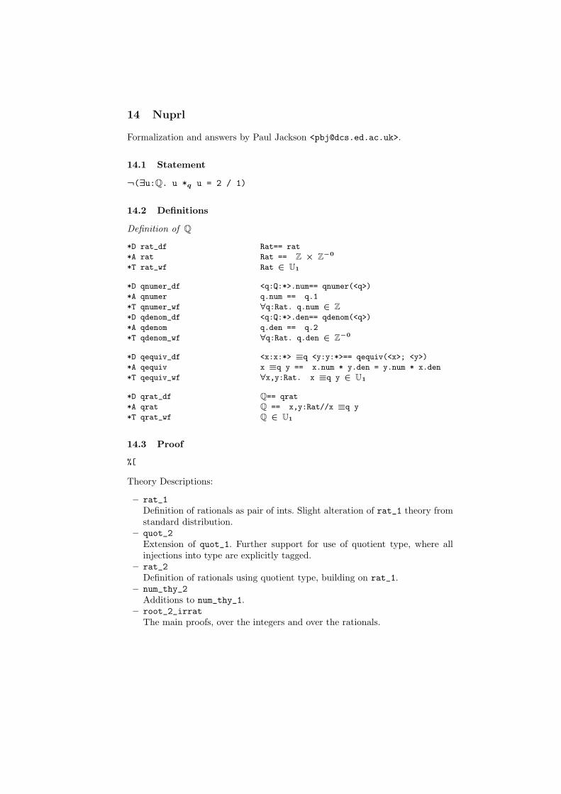
14 Nuprl
Formalization and answers by Paul Jackson <[email protected]>.
14.1 Statement
¬(∃u:Q. u *q u = 2 / 1)
14.2 Definitions
Definition of Q
*D rat_df Rat== rat
*A rat Rat == Z × Z−0
*T rat_wf Rat ∈ U1
*D qnumer_df <q:Q:*>.num== qnumer(<q>)
*A qnumer q.num == q.1
*T qnumer_wf ∀q:Rat. q.num ∈ Z
*D qdenom_df <q:Q:*>.den== qdenom(<q>)
*A qdenom q.den == q.2
*T qdenom_wf ∀q:Rat. q.den ∈ Z−0
*D qequiv_df <x:x:*> ≡q <y:y:*>== qequiv(<x>; <y>)
*A qequiv x ≡q y == x.num * y.den = y.num * x.den
*T qequiv_wf ∀x,y:Rat. x ≡q y ∈ U1
*D qrat_df Q== qrat
*A qrat Q == x,y:Rat//x ≡q y
*T qrat_wf Q ∈ U1
14.3 Proof
%[
Theory Descriptions:
– rat_1
Definition of rationals as pair of ints. Slight alteration of rat_1 theory fromstandard distribution.
– quot_2
Extension of quot_1. Further support for use of quotient type, where allinjections into type are explicitly tagged.
– rat_2
Definition of rationals using quotient type, building on rat_1.– num_thy_2
Additions to num_thy_1.– root_2_irrat
The main proofs, over the integers and over the rationals.

128 Paul Jackson
]%
set_theory_filenames wdir ["rat_1"] ;;
set_theory_filenames wdir ["quot_2"] ;;
set_theory_filenames wdir ["rat_2"] ;;
set_theory_filenames wdir ["num_thy_2"] ;;
set_theory_filenames wdir ["root_2_irrat"] ;;
set_theory_ancestors "rat_1" ["STD"];;
set_theory_ancestors "quot_2" ["STD"];;
set_theory_ancestors "num_thy_2" ["STD"];;
set_theory_ancestors "rat_2" ["rat_1";"quot_2"];;
set_theory_ancestors "root_2_irrat" ["rat_2";"num_thy_2"];;
File root 2 irrat.prl:
*C root_2_irrat_begin ************ ROOT_2_IRRAT ************
*T qrat_irreduc_witness ∀u:Q. ↓(∃n:Z. ∃d:Z−0. u = n / d ∧ CoPrime(n,d))
*T exists_zero_one_elim ∀P:N2 → P. (∃i:N2. P[i]) ⇐⇒ P[0] ∨ P[1]
*T two_div_square ∀n:Z. 2 | n * n ⇒ 2 | n
*T root_2_irrat_over_int ¬(∃m,n:Z. CoPrime(m,n) ∧ m * m = 2 * n * n)
*T root_2_irrat ¬(∃u:Q. u *q u = 2 / 1)
*C root_2_irrat_end **************************************
Proof of qrat irreduc witness:
` ∀u:Q. ↓(∃n:Z. ∃d:Z−0. u = n / d ∈ Q ∧ CoPrime(n,d))
|
BY (D 0 THENM InstLemma ‘qrat_witness‘ [due]
| THENM D 2 THENM D 0 THENM ExRepD ...a)
|
1. u: Q
2. n: Z
3. d: Z−0
4. u = n / d ∈ Q
` ∃n:Z. ∃d:Z−0. u = n / d ∈ Q ∧ CoPrime(n,d)
|
BY % Facts to help type-checking %
|
| (Assert dgcd(n;d) 6= 0e THENA
| (D 0 THENM Sel (-1) (FLemma ‘gcd_zero_result‘ [5]) ...))
| THEN
| (Assert dd ÷ gcd(n;d) 6= 0e THENA
| (Backchain ‘‘div_zero_a gcd_is_divisor_2‘‘ ...))
|
5. gcd(n;d) 6= 0
6. d ÷ gcd(n;d) 6= 0
|
BY (Inst [dn ÷ gcd(n;d)e;dd ÷ gcd(n;d)e] 0 ...a)
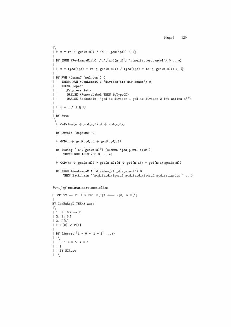
Nuprl 129
|\| ` u = (n ÷ gcd(n;d)) / (d ÷ gcd(n;d)) ∈ Q
| |
| BY (RWH (RevLemmaWithC [‘n’,dgcd(n;d)e] ‘numq_factor_cancel‘) 0 ...a)
| |
| ` u = (gcd(n;d) * (n ÷ gcd(n;d))) / (gcd(n;d) * (d ÷ gcd(n;d))) ∈ Q
| |
| BY RWH (LemmaC ‘mul_com‘) 0
| | THENM RWH (GenLemmaC 1 ‘divides_iff_div_exact‘) 0
| | THENA Repeat
| | (Progress Auto
| | ORELSE (RemoveLabel THEN EqTypeCD)
| | ORELSE Backchain ‘‘gcd_is_divisor_1 gcd_is_divisor_2 int_entire_a‘‘)
| |
| ` u = n / d ∈ Q
| |
| BY Auto
\` CoPrime(n ÷ gcd(n;d),d ÷ gcd(n;d))
|
BY Unfold ‘coprime‘ 0
|
` GCD(n ÷ gcd(n;d);d ÷ gcd(n;d);1)
|
BY (Using [‘n’,dgcd(n;d)e] (BLemma ‘gcd_p_mul_elim‘)
| THENM RWH IntSimpC 0 ...a)
|
` GCD((n ÷ gcd(n;d)) * gcd(n;d);(d ÷ gcd(n;d)) * gcd(n;d);gcd(n;d))
|
BY (RWH (GenLemmaC 1 ‘divides_iff_div_exact‘) 0
THEN Backchain ‘‘gcd_is_divisor_1 gcd_is_divisor_2 gcd_sat_gcd_p‘‘ ...)
Proof of exists zero one elim:
` ∀P:N2 → P. (∃i:N2. P[i]) ⇐⇒ P[0] ∨ P[1]
|
BY GenExRepD THENA Auto
|\| 1. P: N2 → P
| 2. i: N2
| 3. P[i]
| ` P[0] ∨ P[1]
| |
| BY (Assert di = 0 ∨ i = 1e ...a)
| |\| | ` i = 0 ∨ i = 1
| | |
| | BY SIAuto
| \
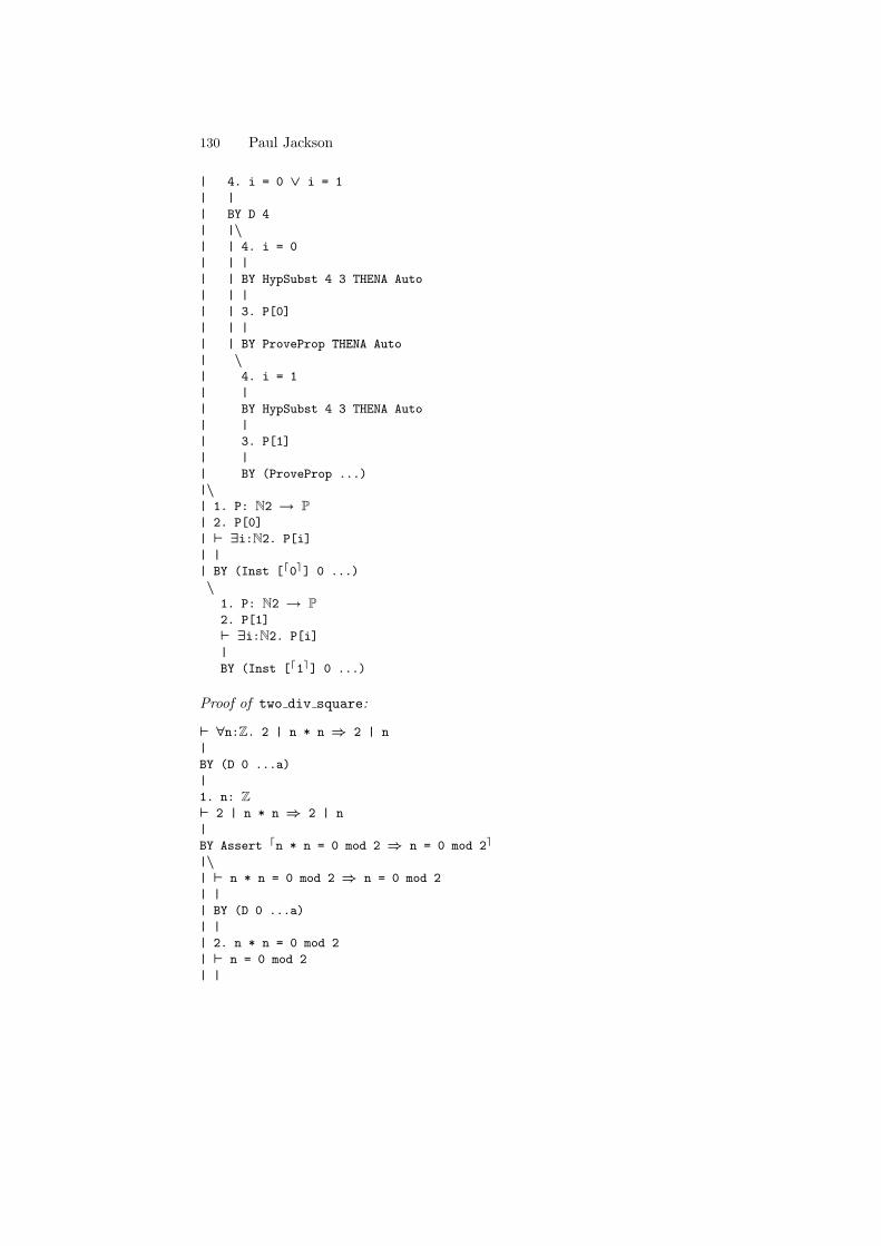
130 Paul Jackson
| 4. i = 0 ∨ i = 1
| |
| BY D 4
| |\| | 4. i = 0
| | |
| | BY HypSubst 4 3 THENA Auto
| | |
| | 3. P[0]
| | |
| | BY ProveProp THENA Auto
| \| 4. i = 1
| |
| BY HypSubst 4 3 THENA Auto
| |
| 3. P[1]
| |
| BY (ProveProp ...)
|\| 1. P: N2 → P
| 2. P[0]
| ` ∃i:N2. P[i]
| |
| BY (Inst [d0e] 0 ...)
\1. P: N2 → P
2. P[1]
` ∃i:N2. P[i]
|
BY (Inst [d1e] 0 ...)
Proof of two div square:
` ∀n:Z. 2 | n * n ⇒ 2 | n
|
BY (D 0 ...a)
|
1. n: Z
` 2 | n * n ⇒ 2 | n
|
BY Assert dn * n = 0 mod 2 ⇒ n = 0 mod 2e
|\| ` n * n = 0 mod 2 ⇒ n = 0 mod 2
| |
| BY (D 0 ...a)
| |
| 2. n * n = 0 mod 2
| ` n = 0 mod 2
| |
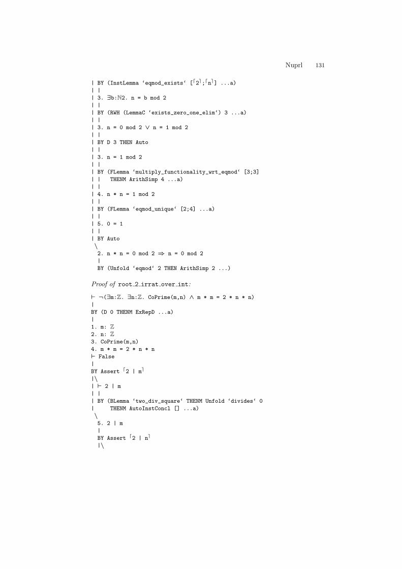
Nuprl 131
| BY (InstLemma ‘eqmod_exists‘ [d2e;dne] ...a)
| |
| 3. ∃b:N2. n = b mod 2
| |
| BY (RWH (LemmaC ‘exists_zero_one_elim‘) 3 ...a)
| |
| 3. n = 0 mod 2 ∨ n = 1 mod 2
| |
| BY D 3 THEN Auto
| |
| 3. n = 1 mod 2
| |
| BY (FLemma ‘multiply_functionality_wrt_eqmod‘ [3;3]
| | THENM ArithSimp 4 ...a)
| |
| 4. n * n = 1 mod 2
| |
| BY (FLemma ‘eqmod_unique‘ [2;4] ...a)
| |
| 5. 0 = 1
| |
| BY Auto
\2. n * n = 0 mod 2 ⇒ n = 0 mod 2
|
BY (Unfold ‘eqmod‘ 2 THEN ArithSimp 2 ...)
Proof of root 2 irrat over int:
` ¬(∃m:Z. ∃n:Z. CoPrime(m,n) ∧ m * m = 2 * n * n)
|
BY (D 0 THENM ExRepD ...a)
|
1. m: Z
2. n: Z
3. CoPrime(m,n)
4. m * m = 2 * n * n
` False
|
BY Assert d2 | me
|\| ` 2 | m
| |
| BY (BLemma ‘two_div_square‘ THENM Unfold ‘divides‘ 0
| THENM AutoInstConcl [] ...a)
\5. 2 | m
|
BY Assert d2 | ne
|\
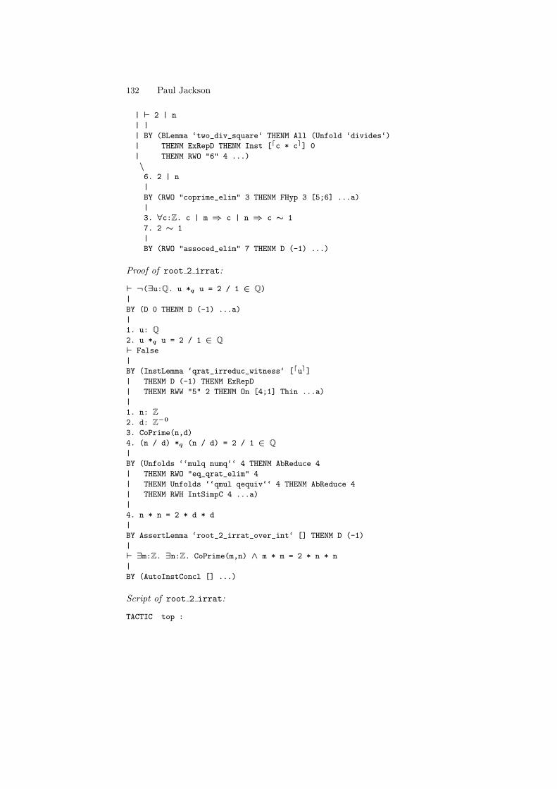
132 Paul Jackson
| ` 2 | n
| |
| BY (BLemma ‘two_div_square‘ THENM All (Unfold ‘divides‘)
| THENM ExRepD THENM Inst [dc * ce] 0
| THENM RWO "6" 4 ...)
\6. 2 | n
|
BY (RWO "coprime_elim" 3 THENM FHyp 3 [5;6] ...a)
|
3. ∀c:Z. c | m ⇒ c | n ⇒ c ∼ 1
7. 2 ∼ 1
|
BY (RWO "assoced_elim" 7 THENM D (-1) ...)
Proof of root 2 irrat:
` ¬(∃u:Q. u *q u = 2 / 1 ∈ Q)
|
BY (D 0 THENM D (-1) ...a)
|
1. u: Q
2. u *q u = 2 / 1 ∈ Q
` False
|
BY (InstLemma ‘qrat_irreduc_witness‘ [due]
| THENM D (-1) THENM ExRepD
| THENM RWW "5" 2 THENM On [4;1] Thin ...a)
|
1. n: Z
2. d: Z−0
3. CoPrime(n,d)
4. (n / d) *q (n / d) = 2 / 1 ∈ Q
|
BY (Unfolds ‘‘mulq numq‘‘ 4 THENM AbReduce 4
| THENM RWO "eq_qrat_elim" 4
| THENM Unfolds ‘‘qmul qequiv‘‘ 4 THENM AbReduce 4
| THENM RWH IntSimpC 4 ...a)
|
4. n * n = 2 * d * d
|
BY AssertLemma ‘root_2_irrat_over_int‘ [] THENM D (-1)
|
` ∃m:Z. ∃n:Z. CoPrime(m,n) ∧ m * m = 2 * n * n
|
BY (AutoInstConcl [] ...)
Script of root 2 irrat:
TACTIC top :
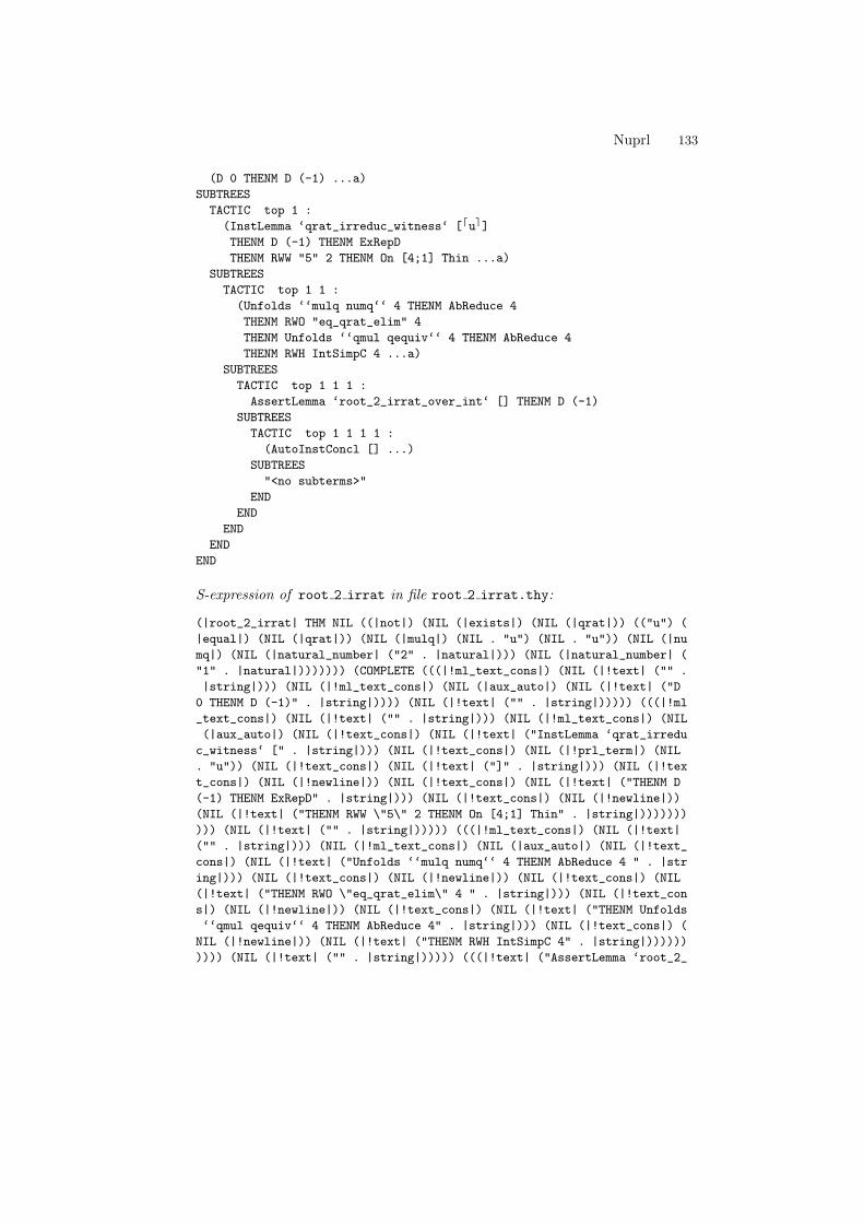
Nuprl 133
(D 0 THENM D (-1) ...a)
SUBTREES
TACTIC top 1 :
(InstLemma ‘qrat_irreduc_witness‘ [due]
THENM D (-1) THENM ExRepD
THENM RWW "5" 2 THENM On [4;1] Thin ...a)
SUBTREES
TACTIC top 1 1 :
(Unfolds ‘‘mulq numq‘‘ 4 THENM AbReduce 4
THENM RWO "eq_qrat_elim" 4
THENM Unfolds ‘‘qmul qequiv‘‘ 4 THENM AbReduce 4
THENM RWH IntSimpC 4 ...a)
SUBTREES
TACTIC top 1 1 1 :
AssertLemma ‘root_2_irrat_over_int‘ [] THENM D (-1)
SUBTREES
TACTIC top 1 1 1 1 :
(AutoInstConcl [] ...)
SUBTREES
"<no subterms>"
END
END
END
END
END
S-expression of root 2 irrat in file root 2 irrat.thy:
(|root_2_irrat| THM NIL ((|not|) (NIL (|exists|) (NIL (|qrat|)) (("u") (
|equal|) (NIL (|qrat|)) (NIL (|mulq|) (NIL . "u") (NIL . "u")) (NIL (|nu
mq|) (NIL (|natural_number| ("2" . |natural|))) (NIL (|natural_number| (
"1" . |natural|))))))) (COMPLETE (((|!ml_text_cons|) (NIL (|!text| ("" .
|string|))) (NIL (|!ml_text_cons|) (NIL (|aux_auto|) (NIL (|!text| ("D
0 THENM D (-1)" . |string|)))) (NIL (|!text| ("" . |string|))))) (((|!ml
_text_cons|) (NIL (|!text| ("" . |string|))) (NIL (|!ml_text_cons|) (NIL
(|aux_auto|) (NIL (|!text_cons|) (NIL (|!text| ("InstLemma ‘qrat_irredu
c_witness‘ [" . |string|))) (NIL (|!text_cons|) (NIL (|!prl_term|) (NIL
. "u")) (NIL (|!text_cons|) (NIL (|!text| ("]" . |string|))) (NIL (|!tex
t_cons|) (NIL (|!newline|)) (NIL (|!text_cons|) (NIL (|!text| ("THENM D
(-1) THENM ExRepD" . |string|))) (NIL (|!text_cons|) (NIL (|!newline|))
(NIL (|!text| ("THENM RWW \"5\" 2 THENM On [4;1] Thin" . |string|)))))))
))) (NIL (|!text| ("" . |string|))))) (((|!ml_text_cons|) (NIL (|!text|
("" . |string|))) (NIL (|!ml_text_cons|) (NIL (|aux_auto|) (NIL (|!text_
cons|) (NIL (|!text| ("Unfolds ‘‘mulq numq‘‘ 4 THENM AbReduce 4 " . |str
ing|))) (NIL (|!text_cons|) (NIL (|!newline|)) (NIL (|!text_cons|) (NIL
(|!text| ("THENM RWO \"eq_qrat_elim\" 4 " . |string|))) (NIL (|!text_con
s|) (NIL (|!newline|)) (NIL (|!text_cons|) (NIL (|!text| ("THENM Unfolds
‘‘qmul qequiv‘‘ 4 THENM AbReduce 4" . |string|))) (NIL (|!text_cons|) (
NIL (|!newline|)) (NIL (|!text| ("THENM RWH IntSimpC 4" . |string|))))))
)))) (NIL (|!text| ("" . |string|))))) (((|!text| ("AssertLemma ‘root_2_
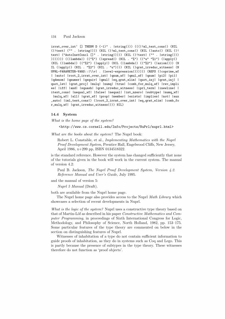
134 Paul Jackson
irrat_over_int‘ [] THENM D (-1)" . |string|))) (((|!ml_text_cons|) (NIL
(|!text| ("" . |string|))) (NIL (|!ml_text_cons|) (NIL (|auto|) (NIL (|!
text| ("AutoInstConcl []" . |string|)))) (NIL (|!text| ("" . |string|)))
))))))) ((|lambda|) (("%") (|spread|) (NIL . "%") (("u" "%1") (|apply|)
(NIL (|lambda|) (("%2") (|apply|) (NIL (|lambda|) (("%2") (|axiom|))) (N
IL (|apply|) (NIL . "%2") (NIL . "u")))) (NIL (|qrat_irreduc_witness| (N
UPRL-PARAMETER-VARS::|\\v| . |level-expression|)))))) (REFS (|coprime_wf
| |auto| |root_2_irrat_over_int| |qnum_wf| |qmul_wf| |qnum| |pi2| |pi1|
|qdenom| |qnumer| |qequiv| |qmul| |eq_qrat_elim| |quot_inj| |qrat_inj| |
quot_let| |qrat_proj| |mulq| |numq| |true| |comb_for_mulq_wf| |rev_impli
es| |iff| |and| |squash| |qrat_irreduc_witness| |iprl_term| |inewline| |
itext_cons| |nequal_wf| |false| |nequal| |int_nzero| |subtype| |numq_wf|
|mulq_wf| |all| |qrat_wf| |prop| |member| |exists| |implies| |not| |aux
_auto| |iml_text_cons|) (|root_2_irrat_over_int| |eq_qrat_elim| |comb_fo
r_mulq_wf| |qrat_irreduc_witness|))) NIL)
14.4 System
What is the home page of the system?
<http://www.cs.cornell.edu/Info/Projects/NuPrl/nuprl.html>
What are the books about the system? The Nuprl book:
Robert L. Constable, et al., Implementing Mathematics with the NuprlProof Development System, Prentice Hall, Engelwood Cliffs, New Jersey,April 1986, x+299 pp, ISBN 0134518322.
is the standard reference. However the system has changed sufficiently that noneof the tutorials given in the book will work in the current system. The manualof version 4.2:
Paul B. Jackson, The Nuprl Proof Development System, Version 4.2.Reference Manual and User’s Guide, July 1995.
and the manual of version 5:
Nuprl 5 Manual (Draft).
both are available from the Nuprl home page.The Nuprl home page also provides access to the Nuprl Math Library which
showcases a selection of recent developments in Nuprl.
What is the logic of the system? Nuprl uses a constructive type theory based onthat of Martin-Lof as described in his paper Constructive Mathematics and Com-puter Programming, in proceedings of Sixth International Congress for Logic,Methodology, and Philosophy of Science, North Holland, 1982, pp. 153–175.Some particular features of the type theory are commented on below in thesection on distinguishing features of Nuprl.
Witnesses of inhabitation of a type do not contain sufficient information toguide proofs of inhabitation, as they do in systems such as Coq and Lego. Thisis partly because the presence of subtypes in the type theory. These witnessestherefore do not function as ‘proof objects’.
Nuprl 135
What is the implementation architecture of the system? Nuprl has an LCF archi-tecture based on an abstract data type of proofs. This proof datatype maintainsthe structure of both incomplete and complete proofs, down to the level of primi-tive inferences if desired. The implementation of the datatype is not as small as inHOL or Isabelle. For example, it has primitive rules for arithmetic simplificationand deciding linear arithmetic problems.
Nuprl has an extensive tactic collection covering operations such as type-checking, rewriting, forward and backward chaining, arithmetic reasoning andinequality reasoning. Tactics are written in Edinburgh ML.
Nuprl 4.2 is implemented in Common Lisp and the 1979 Edinburgh ML.
What does working with the system look like? Proofs are developed interactivelyby running tactics in a proof tree editor. With this editor, one focuses on onenode of the proof tree at a time. The editor presents the user with the full sequentfor the node, together with, if any, the tactic run on that node and the childrenproof nodes generated by the tactic. The Nuprl Math Library presents proofsusing views similar to those generated by this proof tree editor.
All Nuprl expressions are entered using a structure editor and presented onthe screen and in print using syntax chosen for brevity and clarity. There are norequirements that display syntax be parsable. The structure editor is also usedfor the ML tactics: for example, the ... notation is used in display forms forinvocations of Nuprl’s typechecking and basic-reasoning tactic.
With Nuprl 4.2 one typically has
– 1 scrollable library window, listing loaded theorems, definitions, displayforms, comments, and ML objects.
– 1 ML top loop window– For each proof (many proofs can be open simultaneously)
1 proof tree editor window as described above.The proof refinement window is read only.
– To enter main goals of theorems, or enter tactics when developing proofs, onepops up temporary ‘term editor’ windows which permit structure editing.Term editor windows are also used for displaying and editing definitions anddisplay forms, and for the ML top loop (one needs to be able to enter Nuprlterm arguments to tactics).
Proofs are saved to files in the form of proof scripts, recording the tactics usedto generate the proofs.
Definitions, theorems, ML code and comments are grouped together in the-ories. Each theory is saved in a single .thy file using Lisp S-expression syntax.This syntax is verbose and low-level, and users rarely view or edit these filesdirectly with a text editor.
What is special about the system compared to other systems?
– The type theory includes less-common subtype and quotient type type con-structors, and, since 1995, very-dependent function types, where the type of
136 Paul Jackson
the value of the function on some argument can depend on its value on otherarguments smaller in some well-founded order.
– Having subtypes defined by arbitrary predicates makes type checking un-decidable, and all type checking is done by proof. This contrasts with PVSwhere a type-checking algorithm automates all simpler type-checking tasks.Caching of type-checking obligations improves the efficiency of type-checkingby proof.
– The computation language is untyped, enabling the expression of polymor-phic functions without dummy type arguments and the definition of generalrecursive functions with the Y combinator.
– Structure editors are used for all interaction with the system. This permitsthe use of rich syntaxes for terms, proofs and theories that don’t have tobe mechanically parsable. Any ambiguities in syntax are easily resolved byinteraction with the editors.
– Proofs are edited and viewed as proof trees, rather than, for example, goalstacks.
What are other versions of the system? The proofs described here have beencarried out in Nuprl 4.2 which dates from about 1995. There are more recentversions of Nuprl (Nuprl 5, MetaPrl) with significant developments in the userinterface, type theory, and performance, but the level of automation in theseversions is mostly not much different from that shown above. Further detailscan be found from the Nuprl home page.
The Nuprl Math Library pages accessible from the home page illustrate on-going work in producing readable presentations of formal mathematics.
Who are the people behind the system? The principal people involved in thedesign and implementation of Nuprl 4 were Bob Constable, Stuart Allen, RichardEaton, Jason Hickey, Doug Howe and Paul Jackson. Many others were involvedin previous versions.
What are the main user communities of the system? The main users of Nuprlare virtually all existing or former members of the Nuprl group at Cornell.
What large mathematical formalizations have been done in the system? Specificdevelopments, roughly ordered from more purely mathematical to more appliedinclude:
– Constructive real analysis: the intermediate value theorem (Howe, Chirimar1991, Forester 1993)
– Computational abstract algebra: multivariate polynomial arithmetic, uniquefactorisation domains (Jackson 1995)
– Girard’s paradox (Howe 1987)– Metatheory of propositional logics (Caldwell, Gent, Underwood 1990-2001)– Computational metatheory (Howe 1988)– Extracting constructive content from classical proofs: Higman’s Lemma
(Murthy 1991)
Nuprl 137
– Automata theory, Turing machines (Bickford, Constable, Kreitz, Nogin,Naumov, Jackson, Uribe 1986-2001)
See the Nuprl home pages (both publications and Math Library pages) for fullcitations and further details.
What representation of the formalization has been put in this paper? Proofs areshown above in one of the formats commonly used for full proofs. For brevity,each sequent in the tree is shown only with those hypotheses and conclusionformulae and types that have changed from ancestor sequents in the tree.
Proofs are saved to files in the form of proof scripts. As an example, the proofsection shows the usual display of the proof script for root 2 irrat. This is howscripts are displayed interactively when one wants to edit directly an existingscript. The ‘top 1 2 3’ addresses are automatically filled in. These aren’t savedwhen scripts are saved.
What needs to be explained about this specific proof? The proof follows thetraditional approach that is ascribed to Pythagoras and that Lamport chosefor his 1993 DEC SRC report How to Write a Proof.
This Nuprl V4.2 development relies on slight modifications and extensions ofstandard V4.2 theories concerning number theory and the rationals. In particu-lar, whereas the standard theory stops with a definition of the rationals as pairsof integers, here we take here the extra step of using Nuprl’s quotient type toconstruct a more abstract and elegant rational type:
rat:
Rat == Z × Z−0
qequiv:
x ≡q y == x.num * y.den = y.num * x.den
qrat:
Q == x,y:Rat//x ≡q y
For constructivity reasons, elements of quotient types in Nuprl are single repre-sentatives of equivalence classes rather than the equivalence classes themselves.When functions are typed with Q rather than Rat, the type theory requires thefunctions to respect the standard equality on rationals. For example, the typinglemma for the function Q is:
mulq_wf:
∀u:Q. ∀v:Q. u *q v ∈ Q
Any proof of this typing lemma must not only show that the function returnsan element of Q for arguments in Q, but also that it returns equivalent rationalsfor equivalent arguments.
The proofs presented above are revisions of the proofs as originally entered:steps have been combined to reduce the lengths of the proofs and emphasizethe main steps of the proofs. For comparison, the two div square proof has notbeen revised.
138 Paul Jackson
The proof of qrat irreduc witness is complicated by the fact that NuprlV4.2’s tactics don’t handle subtypes as well as, for example, PVS. Integer division(the ÷ operation) is only well-formed for non-zero second arguments, and thetactics need explicit help from the user to prove this.
The ↓ operator in
qrat_irreduc_witness:
∀u:Q. ↓(∃n:Z. ∃d:Z−0. u = n / d ∈ Q ∧ CoPrime(n,d))
is called squash. The type ↓T is a singleton type if T is inhabited, otherwise it isan empty type. The lemma is slightly simpler to prove with the squash operationincluded than without. Without, the proof must exhibit a function, implicitly orexplicitly, that computes the same numerator n and denominator d for any pairof equal rational numbers u. In other words, the proof must involve computingcanonical forms of rational numbers and showing these forms are unique.
The full Nuprl theory and ML files for this work are available online at<http://www.dcs.ed.ac.uk/home/pbj/nuprl>.
The Nuprl Math Library contains an alternate proof of the irrationality of√
2produced by Stuart Allen. This alternate proof does not involve the rationals,but does show the irrationality of square roots of arbitrary primes.
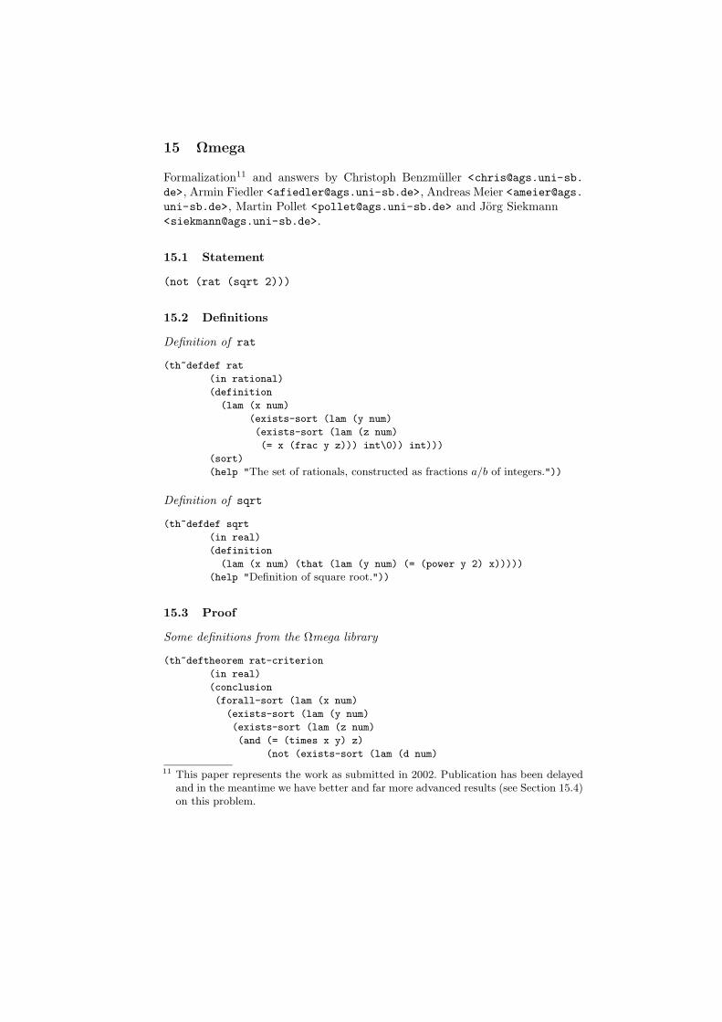
15 Ωmega
Formalization11 and answers by Christoph Benzmuller <[email protected].
de>, Armin Fiedler <[email protected]>, Andreas Meier <[email protected]>, Martin Pollet <[email protected]> and Jorg Siekmann<[email protected]>.
15.1 Statement
(not (rat (sqrt 2)))
15.2 Definitions
Definition of rat
(th~defdef rat
(in rational)
(definition
(lam (x num)
(exists-sort (lam (y num)
(exists-sort (lam (z num)
(= x (frac y z))) int\0)) int)))
(sort)
(help "The set of rationals, constructed as fractions a/b of integers."))
Definition of sqrt
(th~defdef sqrt
(in real)
(definition
(lam (x num) (that (lam (y num) (= (power y 2) x)))))
(help "Definition of square root."))
15.3 Proof
Some definitions from the Ωmega library
(th~deftheorem rat-criterion
(in real)
(conclusion
(forall-sort (lam (x num)
(exists-sort (lam (y num)
(exists-sort (lam (z num)
(and (= (times x y) z)
(not (exists-sort (lam (d num)
11 This paper represents the work as submitted in 2002. Publication has been delayedand in the meantime we have better and far more advanced results (see Section 15.4)on this problem.

140 C. Benzmuller, A. Fiedler, A. Meier, M. Pollet, J. Siekmann
(common-divisor y z d))
int))))
int))
int))
rat))
(help "x rational implies there exist integers y, z which have no commondivisor and furthermore z = x · y."))
(th~deftheorem even-on-integers
(in real)
(conclusion
(forall-sort (lam (x num)
(equiv (evenp x)
(exists-sort (lam (y num)
(= x (times 2 y))) int))) int))
(help "An integer x is even, iff an integer y exists so that x = 2y."))
(th~deftheorem square-even
(in real)
(conclusion
(forall-sort (lam (x num)
(equiv (evenp (power x 2)) (evenp x)))
int))
(help "x is even, iff x2 is even."))
(th~deftheorem even-common-divisor
(in real)
(conclusion
(forall-sort (lam (x num)
(forall-sort (lam (y num)
(implies (and (evenp x) (evenp y))
(common-divisor x y 2)))
int))
int))
(help "If x and y are even, then they have ’2’ as a common divisor."))
(th~deftheorem power-int-closed
(in real)
(conclusion
(forall-sort (lam (x num)
(forall-sort (lam (y num)
(int (power y x)))
int))
int))
(termdecl)
(help "The set of integers is closed under power."))
(th~defproblem sqrt2-not-rat
(in real)
(conclusion (not (rat (sqrt 2))))
(help "√
2 is not a rational number."))
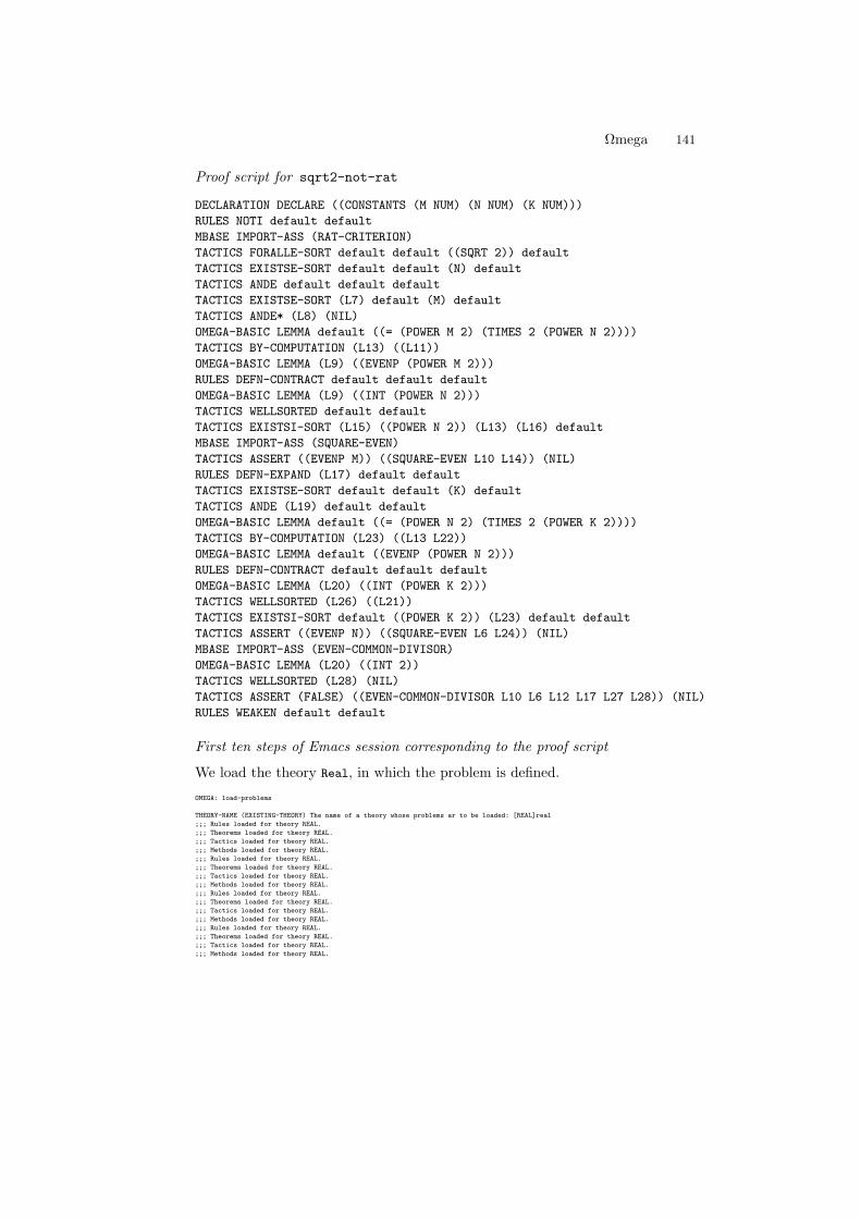
Ωmega 141
Proof script for sqrt2-not-rat
DECLARATION DECLARE ((CONSTANTS (M NUM) (N NUM) (K NUM)))
RULES NOTI default default
MBASE IMPORT-ASS (RAT-CRITERION)
TACTICS FORALLE-SORT default default ((SQRT 2)) default
TACTICS EXISTSE-SORT default default (N) default
TACTICS ANDE default default default
TACTICS EXISTSE-SORT (L7) default (M) default
TACTICS ANDE* (L8) (NIL)
OMEGA-BASIC LEMMA default ((= (POWER M 2) (TIMES 2 (POWER N 2))))
TACTICS BY-COMPUTATION (L13) ((L11))
OMEGA-BASIC LEMMA (L9) ((EVENP (POWER M 2)))
RULES DEFN-CONTRACT default default default
OMEGA-BASIC LEMMA (L9) ((INT (POWER N 2)))
TACTICS WELLSORTED default default
TACTICS EXISTSI-SORT (L15) ((POWER N 2)) (L13) (L16) default
MBASE IMPORT-ASS (SQUARE-EVEN)
TACTICS ASSERT ((EVENP M)) ((SQUARE-EVEN L10 L14)) (NIL)
RULES DEFN-EXPAND (L17) default default
TACTICS EXISTSE-SORT default default (K) default
TACTICS ANDE (L19) default default
OMEGA-BASIC LEMMA default ((= (POWER N 2) (TIMES 2 (POWER K 2))))
TACTICS BY-COMPUTATION (L23) ((L13 L22))
OMEGA-BASIC LEMMA default ((EVENP (POWER N 2)))
RULES DEFN-CONTRACT default default default
OMEGA-BASIC LEMMA (L20) ((INT (POWER K 2)))
TACTICS WELLSORTED (L26) ((L21))
TACTICS EXISTSI-SORT default ((POWER K 2)) (L23) default default
TACTICS ASSERT ((EVENP N)) ((SQUARE-EVEN L6 L24)) (NIL)
MBASE IMPORT-ASS (EVEN-COMMON-DIVISOR)
OMEGA-BASIC LEMMA (L20) ((INT 2))
TACTICS WELLSORTED (L28) (NIL)
TACTICS ASSERT (FALSE) ((EVEN-COMMON-DIVISOR L10 L6 L12 L17 L27 L28)) (NIL)
RULES WEAKEN default default
First ten steps of Emacs session corresponding to the proof script
We load the theory Real, in which the problem is defined.
OMEGA: load-problems
THEORY-NAME (EXISTING-THEORY) The name of a theory whose problems ar to be loaded: [REAL]real
;;; Rules loaded for theory REAL.
;;; Theorems loaded for theory REAL.
;;; Tactics loaded for theory REAL.
;;; Methods loaded for theory REAL.
;;; Rules loaded for theory REAL.
;;; Theorems loaded for theory REAL.
;;; Tactics loaded for theory REAL.
;;; Methods loaded for theory REAL.
;;; Rules loaded for theory REAL.
;;; Theorems loaded for theory REAL.
;;; Tactics loaded for theory REAL.
;;; Methods loaded for theory REAL.
;;; Rules loaded for theory REAL.
;;; Theorems loaded for theory REAL.
;;; Tactics loaded for theory REAL.
;;; Methods loaded for theory REAL.
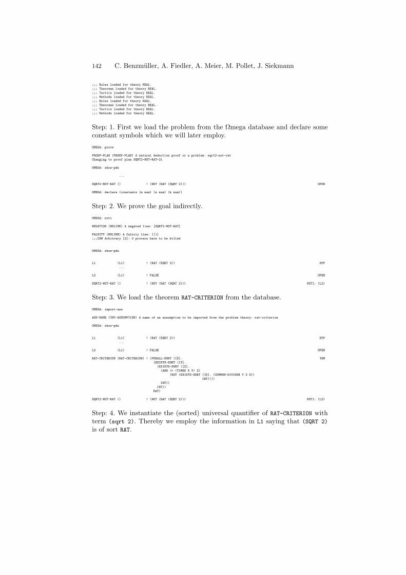
142 C. Benzmuller, A. Fiedler, A. Meier, M. Pollet, J. Siekmann
;;; Rules loaded for theory REAL.
;;; Theorems loaded for theory REAL.
;;; Tactics loaded for theory REAL.
;;; Methods loaded for theory REAL.
;;; Rules loaded for theory REAL.
;;; Theorems loaded for theory REAL.
;;; Tactics loaded for theory REAL.
;;; Methods loaded for theory REAL.
Step: 1. First we load the problem from the Ωmega database and declare someconstant symbols which we will later employ.
OMEGA: prove
PROOF-PLAN (PROOF-PLAN) A natural deduction proof or a problem: sqrt2-not-rat
Changing to proof plan SQRT2-NOT-RAT-21
OMEGA: show-pds
...
SQRT2-NOT-RAT () ! (NOT (RAT (SQRT 2))) OPEN
OMEGA: declare (constants (m num) (n num) (k num))
Step: 2. We prove the goal indirectly.
OMEGA: noti
NEGATION (NDLINE) A negated line: [SQRT2-NOT-RAT]
FALSITY (NDLINE) A falsity line: [()]
;;;CSM Arbitrary [2]: 0 provers have to be killed
OMEGA: show-pds
L1 (L1) ! (RAT (SQRT 2)) HYP
...
L2 (L1) ! FALSE OPEN
SQRT2-NOT-RAT () ! (NOT (RAT (SQRT 2))) NOTI: (L2)
Step: 3. We load the theorem RAT-CRITERION from the database.
OMEGA: import-ass
ASS-NAME (THY-ASSUMPTION) A name of an assumption to be imported from the problem theory: rat-criterion
OMEGA: show-pds
L1 (L1) ! (RAT (SQRT 2)) HYP
...
L2 (L1) ! FALSE OPEN
RAT-CRITERION (RAT-CRITERION) ! (FORALL-SORT ([X]. THM
(EXISTS-SORT ([Y].
(EXISTS-SORT ([Z].
(AND (= (TIMES X Y) Z)
(NOT (EXISTS-SORT ([D]. (COMMON-DIVISOR Y Z D))
INT))))
INT))
INT))
RAT)
SQRT2-NOT-RAT () ! (NOT (RAT (SQRT 2))) NOTI: (L2)
Step: 4. We instantiate the (sorted) universal quantifier of RAT-CRITERION withterm (sqrt 2). Thereby we employ the information in L1 saying that (SQRT 2)
is of sort RAT.
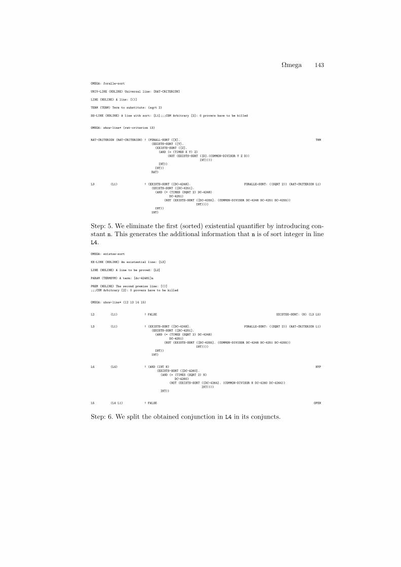
Ωmega 143
OMEGA: foralle-sort
UNIV-LINE (NDLINE) Universal line: [RAT-CRITERION]
LINE (NDLINE) A line: [()]
TERM (TERM) Term to substitute: (sqrt 2)
SO-LINE (NDLINE) A line with sort: [L1];;;CSM Arbitrary [2]: 0 provers have to be killed
OMEGA: show-line* (rat-criterion l3)
RAT-CRITERION (RAT-CRITERION) ! (FORALL-SORT ([X]. THM
(EXISTS-SORT ([Y].
(EXISTS-SORT ([Z].
(AND (= (TIMES X Y) Z)
(NOT (EXISTS-SORT ([D].(COMMON-DIVISOR Y Z D))
INT))))
INT))
INT))
RAT)
L3 (L1) ! (EXISTS-SORT ([DC-4248]. FORALLE-SORT: ((SQRT 2)) (RAT-CRITERION L1)
(EXISTS-SORT ([DC-4251].
(AND (= (TIMES (SQRT 2) DC-4248)
DC-4251)
(NOT (EXISTS-SORT ([DC-4255]. (COMMON-DIVISOR DC-4248 DC-4251 DC-4255))
INT))))
INT))
INT)
Step: 5. We eliminate the first (sorted) existential quantifier by introducing con-stant n. This generates the additional information that n is of sort integer in lineL4.
OMEGA: existse-sort
EX-LINE (NDLINE) An existential line: [L3]
LINE (NDLINE) A line to be proved: [L2]
PARAM (TERMSYM) A term: [dc-42481]n
PREM (NDLINE) The second premise line: [()]
;;;CSM Arbitrary [2]: 0 provers have to be killed
OMEGA: show-line* (l2 l3 l4 l5)
L2 (L1) ! FALSE EXISTSE-SORT: (N) (L3 L5)
L3 (L1) ! (EXISTS-SORT ([DC-4248]. FORALLE-SORT: ((SQRT 2)) (RAT-CRITERION L1)
(EXISTS-SORT ([DC-4251].
(AND (= (TIMES (SQRT 2) DC-4248)
DC-4251)
(NOT (EXISTS-SORT ([DC-4255]. (COMMON-DIVISOR DC-4248 DC-4251 DC-4255))
INT))))
INT))
INT)
L4 (L4) ! (AND (INT N) HYP
(EXISTS-SORT ([DC-4260].
(AND (= (TIMES (SQRT 2) N)
DC-4260)
(NOT (EXISTS-SORT ([DC-4264]. (COMMON-DIVISOR N DC-4260 DC-4264))
INT))))
INT))
L5 (L4 L1) ! FALSE OPEN
Step: 6. We split the obtained conjunction in L4 in its conjuncts.
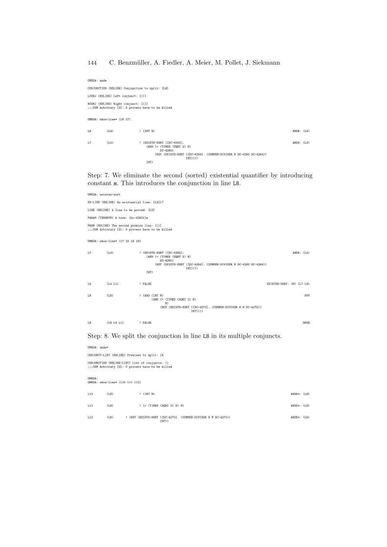
144 C. Benzmuller, A. Fiedler, A. Meier, M. Pollet, J. Siekmann
OMEGA: ande
CONJUNCTION (NDLINE) Conjunction to split: [L4]
LCONJ (NDLINE) Left conjunct: [()]
RCONJ (NDLINE) Right conjunct: [()]
;;;CSM Arbitrary [2]: 0 provers have to be killed
OMEGA: show-line* (l6 l7)
L6 (L4) ! (INT N) ANDE: (L4)
L7 (L4) ! (EXISTS-SORT ([DC-4260]. ANDE: (L4)
(AND (= (TIMES (SQRT 2) N)
DC-4260)
(NOT (EXISTS-SORT ([DC-4264]. (COMMON-DIVISOR N DC-4260 DC-4264))
INT))))
INT)
Step: 7. We eliminate the second (sorted) existential quantifier by introducingconstant m. This introduces the conjunction in line L8.
OMEGA: existse-sort
EX-LINE (NDLINE) An existential line: [L3]l7
LINE (NDLINE) A line to be proved: [L5]
PARAM (TERMSYM) A term: [dc-42601]m
PREM (NDLINE) The second premise line: [()]
;;;CSM Arbitrary [2]: 0 provers have to be killed
OMEGA: show-line* (l7 l5 l8 l9)
L7 (L4) ! (EXISTS-SORT ([DC-4260]. ANDE: (L4)
(AND (= (TIMES (SQRT 2) N)
DC-4260)
(NOT (EXISTS-SORT ([DC-4264]. (COMMON-DIVISOR N DC-4260 DC-4264))
INT))))
INT)
L5 (L4 L1) ! FALSE EXISTSE-SORT: (M) (L7 L9)
L8 (L8) ! (AND (INT M) HYP
(AND (= (TIMES (SQRT 2) N)
M)
(NOT (EXISTS-SORT ([DC-4270]. (COMMON-DIVISOR N M DC-4270))
INT))))
L9 (L8 L4 L1) ! FALSE OPEN
Step: 8. We split the conjunction in line L8 in its multiple conjuncts.
OMEGA: ande*
CONJUNCT-LIST (NDLINE) Premises to split: l8
CONJUNCTION (NDLINE-LIST) List of conjuncts: ()
;;;CSM Arbitrary [2]: 0 provers have to be killed
OMEGA:
OMEGA: show-line* (l10 l11 l12)
L10 (L8) ! (INT M) ANDE*: (L8)
L11 (L8) ! (= (TIMES (SQRT 2) N) M) ANDE*: (L8)
L12 (L8) ! (NOT (EXISTS-SORT ([DC-4270]. (COMMON-DIVISOR N M DC-4270)) ANDE*: (L8)
INT))
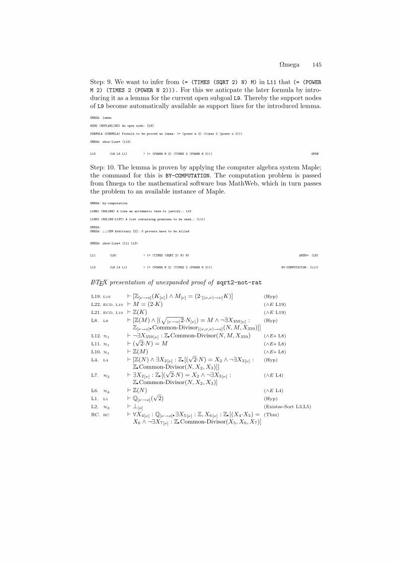
Ωmega 145
Step: 9. We want to infer from (= (TIMES (SQRT 2) N) M) in L11 that (= (POWER
M 2) (TIMES 2 (POWER N 2))). For this we anticpate the later formula by intro-ducing it as a lemma for the current open subgoal L9. Thereby the support nodesof L9 become automatically available as support lines for the introduced lemma.
OMEGA: lemma
NODE (NDPLANLINE) An open node: [L9]
FORMULA (FORMULA) Formula to be proved as lemma: (= (power m 2) (times 2 (power n 2)))
OMEGA: show-line* (l13)
L13 (L8 L4 L1) ! (= (POWER M 2) (TIMES 2 (POWER N 2))) OPEN
Step: 10. The lemma is proven by applying the computer algebra system Maple;the command for this is BY-COMPUTATION. The computation problem is passedfrom Ωmega to the mathematical software bus MathWeb, which in turn passesthe problem to an available instance of Maple.
OMEGA: by-computation
LINE1 (NDLINE) A line an arithmetic term to justify.: l13
LINE2 (NDLINE-LIST) A list containing premises to be used.: (l11)
OMEGA:
OMEGA: ;;;CSM Arbitrary [2]: 0 provers have to be killed
OMEGA: show-line* (l11 l13)
L11 (L8) ! (= (TIMES (SQRT 2) N) M) ANDE*: (L8)
L13 (L8 L4 L1) ! (= (POWER M 2) (TIMES 2 (POWER N 2))) BY-COMPUTATION: (L11)
LATEX presentation of unexpanded proof of sqrt2-not-rat
L19. L19 ` [Z[ν→o](K[ν]) ∧ M[ν] = (2·[(ν,ν)→ν]K)] (Hyp)
L22. ECD, L19 ` M = (2·K) (∧E L19)
L21. ECD, L19 ` Z(K) (∧E L19)
L8. L8 ` [Z(M) ∧ [(p
[ν→ν]2·N[ν]) = M ∧ ¬∃X359[ν] :Z[ν→o] Common-Divisor[(ν,ν,ν)→o](N, M, X359)]]
(Hyp)
L12. H1 ` ¬∃X359[ν] : Z Common-Divisor(N, M, X359) (∧E∗ L8)
L11. H1 ` (√
2·N) = M (∧E∗ L8)
L10. H1 ` Z(M) (∧E∗ L8)
L4. L4 ` [Z(N) ∧ ∃X2[ν] : Z [(√
2·N) = X2 ∧ ¬∃X3[ν] :Z Common-Divisor(N, X2, X3)]]
(Hyp)
L7. H2 ` ∃X2[ν] : Z [(√
2·N) = X2 ∧ ¬∃X3[ν] :Z Common-Divisor(N, X2, X3)]
(∧E L4)
L6. H2 ` Z(N) (∧E L4)
L1. L1 ` Q[ν→o](√
2) (Hyp)
L2. H3 ` ⊥[o] (Existse-Sort L3,L5)
RC. RC ` ∀X4[ν] : Q[ν→o] ∃X5[ν] : Z, X6[ν] : Z [(X4·X5) =X6 ∧ ¬∃X7[ν] : Z Common-Divisor(X5, X6, X7)]
(Thm)
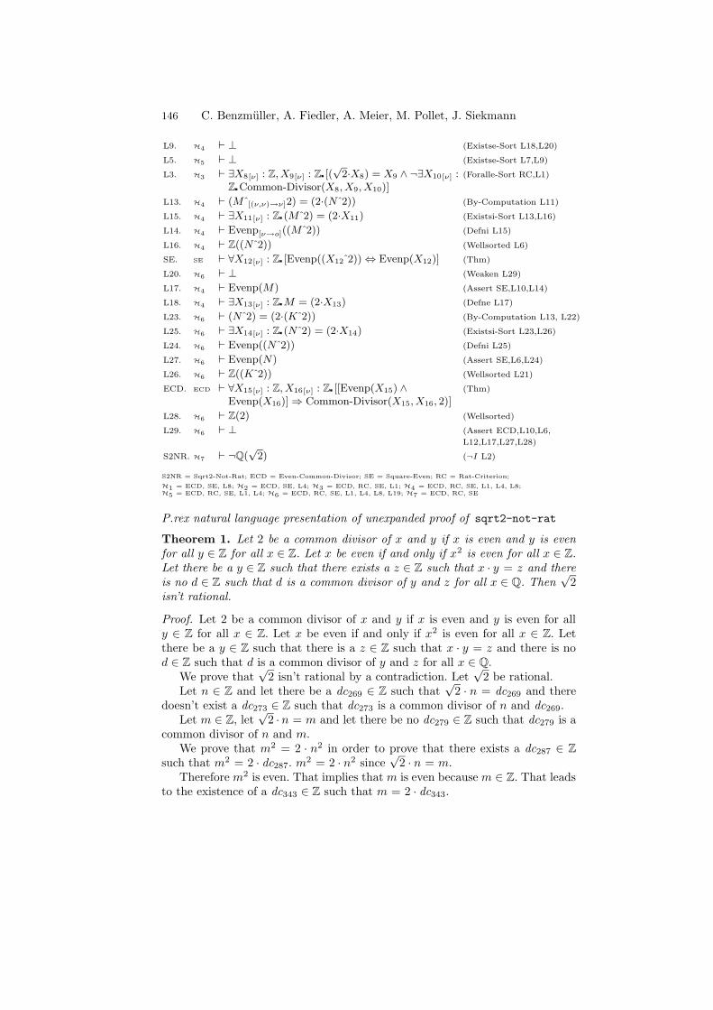
146 C. Benzmuller, A. Fiedler, A. Meier, M. Pollet, J. Siekmann
L9. H4 ` ⊥ (Existse-Sort L18,L20)
L5. H5 ` ⊥ (Existse-Sort L7,L9)
L3. H3 ` ∃X8[ν] : Z, X9[ν] : Z [(√
2·X8) = X9 ∧ ¬∃X10[ν] :Z Common-Divisor(X8, X9, X10)]
(Foralle-Sort RC,L1)
L13. H4 ` (M [(ν,ν)→ν]2) = (2·(N 2)) (By-Computation L11)
L15. H4 ` ∃X11[ν] : Z (M 2) = (2·X11) (Existsi-Sort L13,L16)
L14. H4 ` Evenp[ν→o]((M 2)) (Defni L15)
L16. H4 ` Z((N 2)) (Wellsorted L6)
SE. SE ` ∀X12[ν] : Z [Evenp((X12 2)) ⇔ Evenp(X12)] (Thm)
L20. H6 ` ⊥ (Weaken L29)
L17. H4 ` Evenp(M) (Assert SE,L10,L14)
L18. H4 ` ∃X13[ν] : Z M = (2·X13) (Defne L17)
L23. H6 ` (N 2) = (2·(K 2)) (By-Computation L13, L22)
L25. H6 ` ∃X14[ν] : Z (N 2) = (2·X14) (Existsi-Sort L23,L26)
L24. H6 ` Evenp((N 2)) (Defni L25)
L27. H6 ` Evenp(N) (Assert SE,L6,L24)
L26. H6 ` Z((K 2)) (Wellsorted L21)
ECD. ECD ` ∀X15[ν] : Z, X16[ν] : Z [[Evenp(X15) ∧Evenp(X16)] ⇒ Common-Divisor(X15, X16, 2)]
(Thm)
L28. H6 ` Z(2) (Wellsorted)
L29. H6 ` ⊥ (Assert ECD,L10,L6,
L12,L17,L27,L28)
S2NR. H7 ` ¬Q(√
2) (¬I L2)
S2NR = Sqrt2-Not-Rat; ECD = Even-Common-Divisor; SE = Square-Even; RC = Rat-Criterion;
H1 = ECD, SE, L8; H2 = ECD, SE, L4; H3 = ECD, RC, SE, L1; H4 = ECD, RC, SE, L1, L4, L8;
H5 = ECD, RC, SE, L1, L4; H6 = ECD, RC, SE, L1, L4, L8, L19; H7 = ECD, RC, SE
P.rex natural language presentation of unexpanded proof of sqrt2-not-rat
Theorem 1. Let 2 be a common divisor of x and y if x is even and y is evenfor all y ∈ Z for all x ∈ Z. Let x be even if and only if x2 is even for all x ∈ Z.Let there be a y ∈ Z such that there exists a z ∈ Z such that x · y = z and thereis no d ∈ Z such that d is a common divisor of y and z for all x ∈ Q. Then
√2
isn’t rational.
Proof. Let 2 be a common divisor of x and y if x is even and y is even for ally ∈ Z for all x ∈ Z. Let x be even if and only if x2 is even for all x ∈ Z. Letthere be a y ∈ Z such that there is a z ∈ Z such that x · y = z and there is nod ∈ Z such that d is a common divisor of y and z for all x ∈ Q.
We prove that√
2 isn’t rational by a contradiction. Let√
2 be rational.Let n ∈ Z and let there be a dc269 ∈ Z such that
√2 · n = dc269 and there
doesn’t exist a dc273 ∈ Z such that dc273 is a common divisor of n and dc269.Let m ∈ Z, let
√2 · n = m and let there be no dc279 ∈ Z such that dc279 is a
common divisor of n and m.We prove that m2 = 2 · n2 in order to prove that there exists a dc287 ∈ Z
such that m2 = 2 · dc287. m2 = 2 · n2 since√
2 · n = m.Therefore m2 is even. That implies that m is even because m ∈ Z. That leads
to the existence of a dc343 ∈ Z such that m = 2 · dc343.
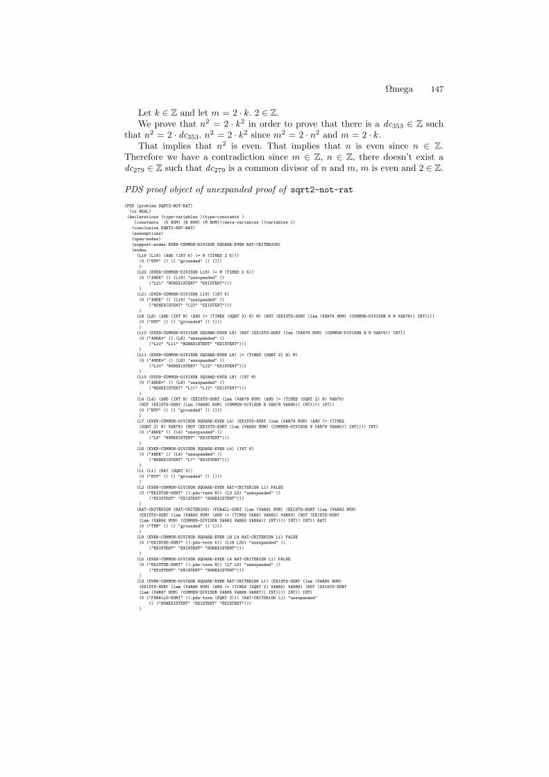
Ωmega 147
Let k ∈ Z and let m = 2 · k. 2 ∈ Z.We prove that n2 = 2 · k2 in order to prove that there is a dc353 ∈ Z such
that n2 = 2 · dc353. n2 = 2 · k2 since m2 = 2 · n2 and m = 2 · k.That implies that n2 is even. That implies that n is even since n ∈ Z.
Therefore we have a contradiction since m ∈ Z, n ∈ Z, there doesn’t exist adc279 ∈ Z such that dc279 is a common divisor of n and m, m is even and 2 ∈ Z.
PDS proof object of unexpanded proof of sqrt2-not-rat
(PDS (problem SQRT2-NOT-RAT)
(in REAL)
(declarations (type-variables )(type-constants )
(constants (K NUM) (N NUM) (M NUM))(meta-variables )(variables ))
(conclusion SQRT2-NOT-RAT)
(assumptions)
(open-nodes)
(support-nodes EVEN-COMMON-DIVISOR SQUARE-EVEN RAT-CRITERION)
(nodes
(L19 (L19) (AND (INT K) (= M (TIMES 2 K)))
(0 ("HYP" () () "grounded" () ()))
)
(L22 (EVEN-COMMON-DIVISOR L19) (= M (TIMES 2 K))
(0 ("ANDE" () (L19) "unexpanded" ()
("L21" "NONEXISTENT" "EXISTENT")))
)
(L21 (EVEN-COMMON-DIVISOR L19) (INT K)
(0 ("ANDE" () (L19) "unexpanded" ()
("NONEXISTENT" "L22" "EXISTENT")))
)
(L8 (L8) (AND (INT M) (AND (= (TIMES (SQRT 2) N) M) (NOT (EXISTS-SORT (lam (VAR76 NUM) (COMMON-DIVISOR N M VAR76)) INT))))
(0 ("HYP" () () "grounded" () ()))
)
(L12 (EVEN-COMMON-DIVISOR SQUARE-EVEN L8) (NOT (EXISTS-SORT (lam (VAR76 NUM) (COMMON-DIVISOR N M VAR76)) INT))
(0 ("ANDE*" () (L8) "unexpanded" ()
("L10" "L11" "NONEXISTENT" "EXISTENT")))
)
(L11 (EVEN-COMMON-DIVISOR SQUARE-EVEN L8) (= (TIMES (SQRT 2) N) M)
(0 ("ANDE*" () (L8) "unexpanded" ()
("L10" "NONEXISTENT" "L12" "EXISTENT")))
)
(L10 (EVEN-COMMON-DIVISOR SQUARE-EVEN L8) (INT M)
(0 ("ANDE*" () (L8) "unexpanded" ()
("NONEXISTENT" "L11" "L12" "EXISTENT")))
)
(L4 (L4) (AND (INT N) (EXISTS-SORT (lam (VAR79 NUM) (AND (= (TIMES (SQRT 2) N) VAR79)
(NOT (EXISTS-SORT (lam (VAR80 NUM) (COMMON-DIVISOR N VAR79 VAR80)) INT)))) INT))
(0 ("HYP" () () "grounded" () ()))
)
(L7 (EVEN-COMMON-DIVISOR SQUARE-EVEN L4) (EXISTS-SORT (lam (VAR79 NUM) (AND (= (TIMES
(SQRT 2) N) VAR79) (NOT (EXISTS-SORT (lam (VAR80 NUM) (COMMON-DIVISOR N VAR79 VAR80)) INT)))) INT)
(0 ("ANDE" () (L4) "unexpanded" ()
("L6" "NONEXISTENT" "EXISTENT")))
)
(L6 (EVEN-COMMON-DIVISOR SQUARE-EVEN L4) (INT N)
(0 ("ANDE" () (L4) "unexpanded" ()
("NONEXISTENT" "L7" "EXISTENT")))
)
(L1 (L1) (RAT (SQRT 2))
(0 ("HYP" () () "grounded" () ()))
)
(L2 (EVEN-COMMON-DIVISOR SQUARE-EVEN RAT-CRITERION L1) FALSE
(0 ("EXISTSE-SORT" ((:pds-term N)) (L3 L5) "unexpanded" ()
("EXISTENT" "EXISTENT" "NONEXISTENT")))
)
(RAT-CRITERION (RAT-CRITERION) (FORALL-SORT (lam (VAR81 NUM) (EXISTS-SORT (lam (VAR82 NUM)
(EXISTS-SORT (lam (VAR83 NUM) (AND (= (TIMES VAR81 VAR82) VAR83) (NOT (EXISTS-SORT
(lam (VAR84 NUM) (COMMON-DIVISOR VAR82 VAR83 VAR84)) INT)))) INT)) INT)) RAT)
(0 ("THM" () () "grounded" () ()))
)
(L9 (EVEN-COMMON-DIVISOR SQUARE-EVEN L8 L4 RAT-CRITERION L1) FALSE
(0 ("EXISTSE-SORT" ((:pds-term K)) (L18 L20) "unexpanded" ()
("EXISTENT" "EXISTENT" "NONEXISTENT")))
)
(L5 (EVEN-COMMON-DIVISOR SQUARE-EVEN L4 RAT-CRITERION L1) FALSE
(0 ("EXISTSE-SORT" ((:pds-term M)) (L7 L9) "unexpanded" ()
("EXISTENT" "EXISTENT" "NONEXISTENT")))
)
(L3 (EVEN-COMMON-DIVISOR SQUARE-EVEN RAT-CRITERION L1) (EXISTS-SORT (lam (VAR85 NUM)
(EXISTS-SORT (lam (VAR86 NUM) (AND (= (TIMES (SQRT 2) VAR85) VAR86) (NOT (EXISTS-SORT
(lam (VAR87 NUM) (COMMON-DIVISOR VAR85 VAR86 VAR87)) INT)))) INT)) INT)
(0 ("FORALLE-SORT" ((:pds-term (SQRT 2))) (RAT-CRITERION L1) "unexpanded"
() ("NONEXISTENT" "EXISTENT" "EXISTENT")))
)
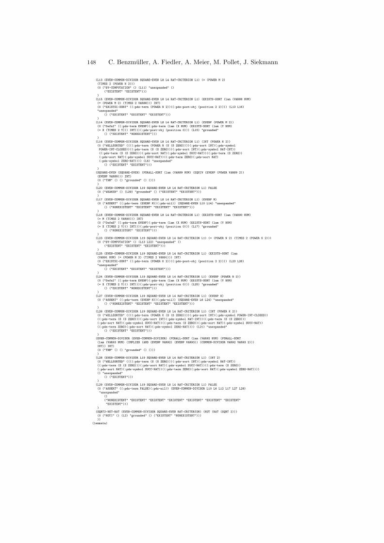
148 C. Benzmuller, A. Fiedler, A. Meier, M. Pollet, J. Siekmann
(L13 (EVEN-COMMON-DIVISOR SQUARE-EVEN L8 L4 RAT-CRITERION L1) (= (POWER M 2)
(TIMES 2 (POWER N 2)))
(0 ("BY-COMPUTATION" () (L11) "unexpanded" ()
("EXISTENT" "EXISTENT")))
)
(L15 (EVEN-COMMON-DIVISOR SQUARE-EVEN L8 L4 RAT-CRITERION L1) (EXISTS-SORT (lam (VAR88 NUM)
(= (POWER M 2) (TIMES 2 VAR88))) INT)
(0 ("EXISTSI-SORT" ((:pds-term (POWER N 2))((:pds-post-obj (position 2 2)))) (L13 L16)
"unexpanded"
() ("EXISTENT" "EXISTENT" "EXISTENT")))
)
(L14 (EVEN-COMMON-DIVISOR SQUARE-EVEN L8 L4 RAT-CRITERION L1) (EVENP (POWER M 2))
(0 ("DefnI" ((:pds-term EVENP)(:pds-term (lam (X NUM) (EXISTS-SORT (lam (Y NUM)
(= X (TIMES 2 Y))) INT)))(:pds-post-obj (position 0))) (L15) "grounded"
() ("EXISTENT" "NONEXISTENT")))
)
(L16 (EVEN-COMMON-DIVISOR SQUARE-EVEN L8 L4 RAT-CRITERION L1) (INT (POWER N 2))
(0 ("WELLSORTED" ((((:pds-term (POWER N (S (S ZERO))))(:pds-sort INT)(:pds-symbol
POWER-INT-CLOSED))((:pds-term (S (S ZERO)))(:pds-sort INT)(:pds-symbol NAT-INT))
((:pds-term (S (S ZERO)))(:pds-sort NAT)(:pds-symbol SUCC-NAT))((:pds-term (S ZERO))
(:pds-sort NAT)(:pds-symbol SUCC-NAT))((:pds-term ZERO)(:pds-sort NAT)
(:pds-symbol ZERO-NAT)))) (L6) "unexpanded"
() ("EXISTENT" "EXISTENT")))
)
(SQUARE-EVEN (SQUARE-EVEN) (FORALL-SORT (lam (VAR89 NUM) (EQUIV (EVENP (POWER VAR89 2))
(EVENP VAR89))) INT)
(0 ("THM" () () "grounded" () ()))
)
(L20 (EVEN-COMMON-DIVISOR L19 SQUARE-EVEN L8 L4 RAT-CRITERION L1) FALSE
(0 ("WEAKEN" () (L29) "grounded" () ("EXISTENT" "EXISTENT")))
)
(L17 (EVEN-COMMON-DIVISOR SQUARE-EVEN L8 L4 RAT-CRITERION L1) (EVENP M)
(0 ("ASSERT" ((:pds-term (EVENP M))(:pds-nil)) (SQUARE-EVEN L10 L14) "unexpanded"
() ("NONEXISTENT" "EXISTENT" "EXISTENT" "EXISTENT")))
)
(L18 (EVEN-COMMON-DIVISOR SQUARE-EVEN L8 L4 RAT-CRITERION L1) (EXISTS-SORT (lam (VAR90 NUM)
(= M (TIMES 2 VAR90))) INT)
(0 ("DefnE" ((:pds-term EVENP)(:pds-term (lam (X NUM) (EXISTS-SORT (lam (Y NUM)
(= X (TIMES 2 Y))) INT)))(:pds-post-obj (position 0))) (L17) "grounded"
() ("NONEXISTENT" "EXISTENT")))
)
(L23 (EVEN-COMMON-DIVISOR L19 SQUARE-EVEN L8 L4 RAT-CRITERION L1) (= (POWER N 2) (TIMES 2 (POWER K 2)))
(0 ("BY-COMPUTATION" () (L13 L22) "unexpanded" ()
("EXISTENT" "EXISTENT" "EXISTENT")))
)
(L25 (EVEN-COMMON-DIVISOR L19 SQUARE-EVEN L8 L4 RAT-CRITERION L1) (EXISTS-SORT (lam
(VAR91 NUM) (= (POWER N 2) (TIMES 2 VAR91))) INT)
(0 ("EXISTSI-SORT" ((:pds-term (POWER K 2))((:pds-post-obj (position 2 2)))) (L23 L26)
"unexpanded"
() ("EXISTENT" "EXISTENT" "EXISTENT")))
)
(L24 (EVEN-COMMON-DIVISOR L19 SQUARE-EVEN L8 L4 RAT-CRITERION L1) (EVENP (POWER N 2))
(0 ("DefnI" ((:pds-term EVENP)(:pds-term (lam (X NUM) (EXISTS-SORT (lam (Y NUM)
(= X (TIMES 2 Y))) INT)))(:pds-post-obj (position 0))) (L25) "grounded"
() ("EXISTENT" "NONEXISTENT")))
)
(L27 (EVEN-COMMON-DIVISOR L19 SQUARE-EVEN L8 L4 RAT-CRITERION L1) (EVENP N)
(0 ("ASSERT" ((:pds-term (EVENP N))(:pds-nil)) (SQUARE-EVEN L6 L24) "unexpanded"
() ("NONEXISTENT" "EXISTENT" "EXISTENT" "EXISTENT")))
)
(L26 (EVEN-COMMON-DIVISOR L19 SQUARE-EVEN L8 L4 RAT-CRITERION L1) (INT (POWER K 2))
(0 ("WELLSORTED" ((((:pds-term (POWER K (S (S ZERO))))(:pds-sort INT)(:pds-symbol POWER-INT-CLOSED))
((:pds-term (S (S ZERO)))(:pds-sort INT)(:pds-symbol NAT-INT))((:pds-term (S (S ZERO)))
(:pds-sort NAT)(:pds-symbol SUCC-NAT))((:pds-term (S ZERO))(:pds-sort NAT)(:pds-symbol SUCC-NAT))
((:pds-term ZERO)(:pds-sort NAT)(:pds-symbol ZERO-NAT)))) (L21) "unexpanded"
() ("EXISTENT" "EXISTENT")))
)
(EVEN-COMMON-DIVISOR (EVEN-COMMON-DIVISOR) (FORALL-SORT (lam (VAR92 NUM) (FORALL-SORT
(lam (VAR93 NUM) (IMPLIES (AND (EVENP VAR92) (EVENP VAR93)) (COMMON-DIVISOR VAR92 VAR93 2)))
INT)) INT)
(0 ("THM" () () "grounded" () ()))
)
(L28 (EVEN-COMMON-DIVISOR L19 SQUARE-EVEN L8 L4 RAT-CRITERION L1) (INT 2)
(0 ("WELLSORTED" ((((:pds-term (S (S ZERO)))(:pds-sort INT)(:pds-symbol NAT-INT))
((:pds-term (S (S ZERO)))(:pds-sort NAT)(:pds-symbol SUCC-NAT))((:pds-term (S ZERO))
(:pds-sort NAT)(:pds-symbol SUCC-NAT))((:pds-term ZERO)(:pds-sort NAT)(:pds-symbol ZERO-NAT))))
() "unexpanded"
() ("EXISTENT")))
)
(L29 (EVEN-COMMON-DIVISOR L19 SQUARE-EVEN L8 L4 RAT-CRITERION L1) FALSE
(0 ("ASSERT" ((:pds-term FALSE)(:pds-nil)) (EVEN-COMMON-DIVISOR L10 L6 L12 L17 L27 L28)
"unexpanded"
()
("NONEXISTENT" "EXISTENT" "EXISTENT" "EXISTENT" "EXISTENT" "EXISTENT" "EXISTENT"
"EXISTENT")))
)
(SQRT2-NOT-RAT (EVEN-COMMON-DIVISOR SQUARE-EVEN RAT-CRITERION) (NOT (RAT (SQRT 2)))
(0 ("NOTI" () (L2) "grounded" () ("EXISTENT" "NONEXISTENT")))
))
(lemmata)
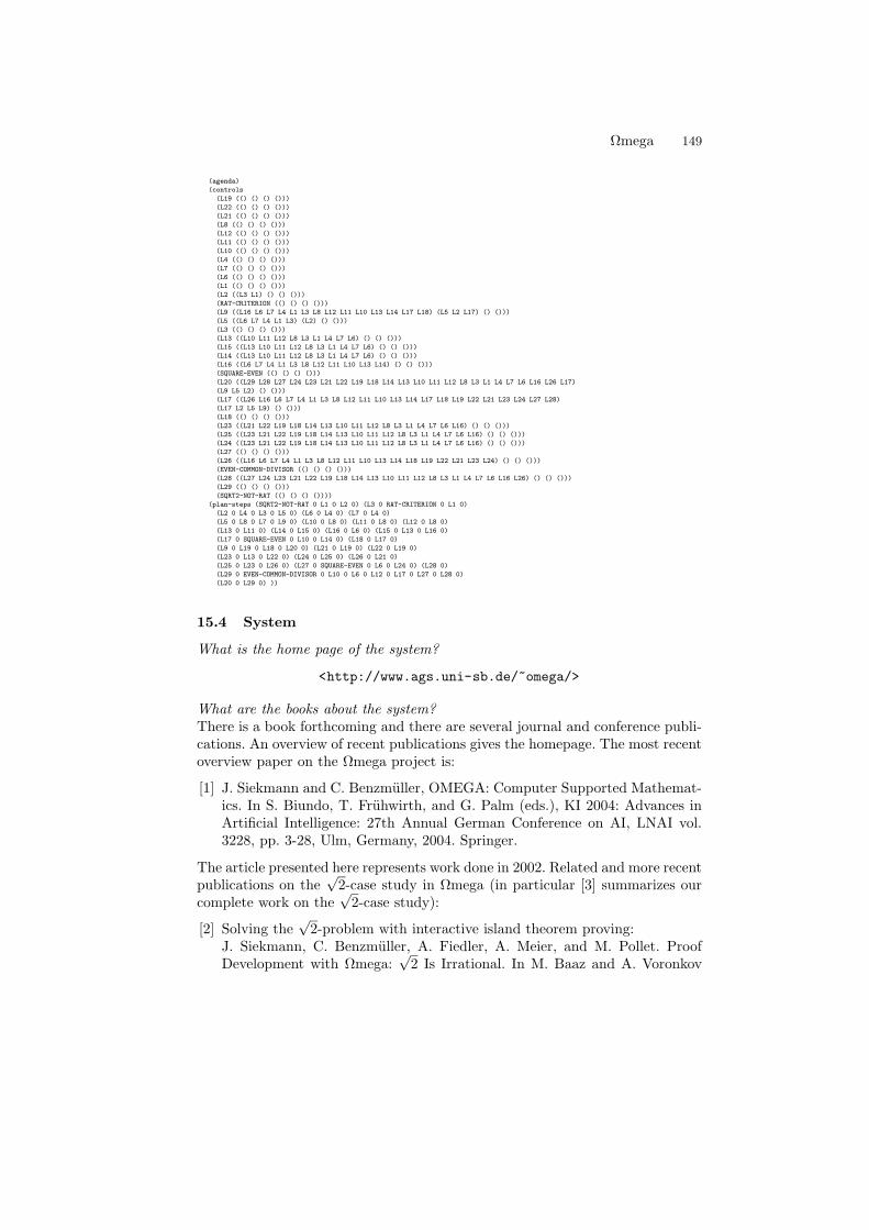
Ωmega 149
(agenda)
(controls
(L19 (() () () ()))
(L22 (() () () ()))
(L21 (() () () ()))
(L8 (() () () ()))
(L12 (() () () ()))
(L11 (() () () ()))
(L10 (() () () ()))
(L4 (() () () ()))
(L7 (() () () ()))
(L6 (() () () ()))
(L1 (() () () ()))
(L2 ((L3 L1) () () ()))
(RAT-CRITERION (() () () ()))
(L9 ((L16 L6 L7 L4 L1 L3 L8 L12 L11 L10 L13 L14 L17 L18) (L5 L2 L17) () ()))
(L5 ((L6 L7 L4 L1 L3) (L2) () ()))
(L3 (() () () ()))
(L13 ((L10 L11 L12 L8 L3 L1 L4 L7 L6) () () ()))
(L15 ((L13 L10 L11 L12 L8 L3 L1 L4 L7 L6) () () ()))
(L14 ((L13 L10 L11 L12 L8 L3 L1 L4 L7 L6) () () ()))
(L16 ((L6 L7 L4 L1 L3 L8 L12 L11 L10 L13 L14) () () ()))
(SQUARE-EVEN (() () () ()))
(L20 ((L29 L28 L27 L24 L23 L21 L22 L19 L18 L14 L13 L10 L11 L12 L8 L3 L1 L4 L7 L6 L16 L26 L17)
(L9 L5 L2) () ()))
(L17 ((L26 L16 L6 L7 L4 L1 L3 L8 L12 L11 L10 L13 L14 L17 L18 L19 L22 L21 L23 L24 L27 L28)
(L17 L2 L5 L9) () ()))
(L18 (() () () ()))
(L23 ((L21 L22 L19 L18 L14 L13 L10 L11 L12 L8 L3 L1 L4 L7 L6 L16) () () ()))
(L25 ((L23 L21 L22 L19 L18 L14 L13 L10 L11 L12 L8 L3 L1 L4 L7 L6 L16) () () ()))
(L24 ((L23 L21 L22 L19 L18 L14 L13 L10 L11 L12 L8 L3 L1 L4 L7 L6 L16) () () ()))
(L27 (() () () ()))
(L26 ((L16 L6 L7 L4 L1 L3 L8 L12 L11 L10 L13 L14 L18 L19 L22 L21 L23 L24) () () ()))
(EVEN-COMMON-DIVISOR (() () () ()))
(L28 ((L27 L24 L23 L21 L22 L19 L18 L14 L13 L10 L11 L12 L8 L3 L1 L4 L7 L6 L16 L26) () () ()))
(L29 (() () () ()))
(SQRT2-NOT-RAT (() () () ())))
(plan-steps (SQRT2-NOT-RAT 0 L1 0 L2 0) (L3 0 RAT-CRITERION 0 L1 0)
(L2 0 L4 0 L3 0 L5 0) (L6 0 L4 0) (L7 0 L4 0)
(L5 0 L8 0 L7 0 L9 0) (L10 0 L8 0) (L11 0 L8 0) (L12 0 L8 0)
(L13 0 L11 0) (L14 0 L15 0) (L16 0 L6 0) (L15 0 L13 0 L16 0)
(L17 0 SQUARE-EVEN 0 L10 0 L14 0) (L18 0 L17 0)
(L9 0 L19 0 L18 0 L20 0) (L21 0 L19 0) (L22 0 L19 0)
(L23 0 L13 0 L22 0) (L24 0 L25 0) (L26 0 L21 0)
(L25 0 L23 0 L26 0) (L27 0 SQUARE-EVEN 0 L6 0 L24 0) (L28 0)
(L29 0 EVEN-COMMON-DIVISOR 0 L10 0 L6 0 L12 0 L17 0 L27 0 L28 0)
(L20 0 L29 0) ))
15.4 System
What is the home page of the system?
<http://www.ags.uni-sb.de/~omega/>
What are the books about the system?There is a book forthcoming and there are several journal and conference publi-cations. An overview of recent publications gives the homepage. The most recentoverview paper on the Ωmega project is:
[1] J. Siekmann and C. Benzmuller, OMEGA: Computer Supported Mathemat-ics. In S. Biundo, T. Fruhwirth, and G. Palm (eds.), KI 2004: Advances inArtificial Intelligence: 27th Annual German Conference on AI, LNAI vol.3228, pp. 3-28, Ulm, Germany, 2004. Springer.
The article presented here represents work done in 2002. Related and more recentpublications on the
√2-case study in Ωmega (in particular [3] summarizes our
complete work on the√
2-case study):
[2] Solving the√
2-problem with interactive island theorem proving:J. Siekmann, C. Benzmuller, A. Fiedler, A. Meier, and M. Pollet. ProofDevelopment with Ωmega:
√2 Is Irrational. In M. Baaz and A. Voronkov
150 C. Benzmuller, A. Fiedler, A. Meier, M. Pollet, J. Siekmann
(eds.), Logic for Programming, Artificial Intelligence, and Reasoning — 9thInternational Conference, LPAR 2002 , number 2514 in LNAI, pp. 367-387,Tbilisi, Georgia, Springer Verlag, 2002.
[3] Solving the√
2-problem (and its generalization) fully automatically withproof planning:J. Siekmann, C. Benzmuller, A. Fiedler, A. Meier, I. Normann, and M. Pollet.Proof Development with Ωmega: The Irrationality of
√2. In F. Kamareddine
(ed.), Thirty Five Years of Automating Mathematics, pp. 271-314, KluwerAcademic Publishers, 2003.
What is the logic of the system?Ωmega employs a higher-order logic based on Church’s simply typed λ-calculus(with prefix-polymorphism). Furthermore, there is a simple sort mechanism inΩmega.
What is the implementation architecture of the system?Ωmega consists of several distributed modules that are connected via the Math-Web mathematical software bus. Different modules are written in different pro-gramming languages (e.g. the Ωmega kernel and the proof planner are writtenin Lisp, the graphical user interface is written in Oz).
What does working with the system look like?There are different modes for the proof search:
1. Interactive Proof Construction with Tactics, Methods, and Calculus Rules.This is the level of proof construction displayed in this paper. Essentially itis like any other interactive, tactic-based theorem prover and definitely notthe level we expect real mathematics to be represented. In fact, the wholepurpose of the Ωmega project is to show that there is a substantially betterway to prove theorems, namely at the proof planning level.
2. Interactive Island Proof Planning.In this mode, the user presents “islands”, that is, intermediate statementsin the potential proof sequence. The system then closes the gaps by proofplanning. See [2] for a report about an island proof of the
√2 problem.
3. Automated Proof Planning.In the best of all worlds the system finds a proof fully automatically by ahierarchical expansion of a high-level proof plan into a low-level logic proof.See [3] for a fully automated solution to the
√2 problem, where we also
introduce and automatically prove its generalization: the irrationality of i√
kfor any i, k ∈ N.
4. Calling External Reasoners via MathWeb.This is important for the
√2 problem as well. Some gaps (subproblems) are
closed by a computer algebra system, simple gaps in an island proof areclosed by (fast and simple) first- and higher-order theorem provers and theproof planner also uses a constraint solver as an external subsystem.
5. Combinations of the above.
Ωmega 151
What is special about the system compared to other systems? The Ωmega systemis a representative system in the new paradigm of proof planning and combinesinteractive and automated proof construction in mathematical domains.
The main purpose of the Ωmega project is to show that computer-supportedmathematics and proving can be done at a more advanced and human-orientedlevel of abstraction as typically found in a mathematical paper or textbook.However, it can be used also just like any other interactive tactic-based system,as this article shows.
Ωmega’s inference mechanism so far has been based on a higher-order naturaldeduction (ND) variant of a sorted version of Church’s simply typed λ-calculus.The user can interactively construct proofs directly at the calculus level or at themore abstract level of tactics (as shown in this article) or proof planning withmethods. Proof construction can be supported by already proven assertions andlemmata and also by calls to external systems to simplify or solve subproblems. Arecent issue in the project is to replace Ωmega’s ND calculus by a more human-oriented, sound and complete base framework that better and more directlysupports reasoning at the logic and assertion level.
At the core of Ωmega is the proof plan data structure PDS in which proofs andproof plans are represented at various levels of granularity and abstraction. Theproof plans are classified with respect to a taxonomy of mathematical theories,which are currently being replaced by the mathematical data base MBase. Theuser of Ωmega, or the proof planner Multi, or the suggestion mechanism Ω-Antsmodify the PDS during proof development. They can invoke external reasoningsystems whose results are included in the PDS after appropriate transformation.After expansion of these high level proofs to the underlying ND calculus, thePDS can be checked by Ωmega’s proof checker. User interaction is supported bythe graphical user interface LΩUI and the translation into natural language bythe proof explainer P.rex.
Several first-order ATPs are connected to Ωmega via Tramp, which is a prooftransformation system that transforms resolution-style proofs into assertion levelND proofs.
What are other versions of the system?The most recent version is Ωmega 3.6.
Who are the people behind the system?The list of Ωmega group members and affiliated researchers includes (many RAswork in Ωmega related research projects and only a few directly on the kernelof the system):
Serge Autexier, Christoph Benzmuller, Chad Brown, Mark Buckley, LassaadCheikhrouhou, Dominik Dietrich, Armin Fiedler, Andreas Franke, Helmut Ho-racek, Mateja Jamnik (now at Cambridge University, Cambridge, UK), ManfredKerber (now at University of Birmingham, Birmingham, UK), Michael Kohlhase(now at International University Bremen, Bremen, Germany), Henri Lesourd,Andreas Meier, Erica Melis, Martin Pollet, Marvin Schiller, Jorg Siekmann,Volker Sorge (now at University of Birmingham, Birmingham, UK), Carsten

152 C. Benzmuller, A. Fiedler, A. Meier, M. Pollet, J. Siekmann
Ullrich, Quoc Bao Vo (now at RMIT University, Melbourne, Australia), MarcWagner, Claus-Peter Wirth, Jurgen Zimmer.
What are the main user communities of the system?The Ωmega system is employed at: Saarland University and the DFKI (AG Siek-mann), the University of Birmingham (Manfred Kerber and Volker Sorge), Inter-national University Bremen (Michael Kohlhase), Cambridge University (MatejaJamnik), University of Edinburgh (Jurgen Zimmer).
What large mathematical formalizations have been done in the system?The Ωmega system has been used in several other case studies, which illustratein particular the interplay of the various components, such as proof planningsupported by heterogeneous external reasoning systems. Publication referencesto these case studies are available in [1] (see above).
A typical example for a class of problems that cannot be solved by traditionalautomated theorem provers is the class of ε–δ–proofs. This class was originallyproposed as a challenge by Woody Bledsoe and it comprises theorems such asLIM+ and LIM*, where LIM+ states that the limit of the sum of two functionsequals the sum of their limits and LIM* makes the corresponding statement formultiplication. The difficulty of this domain arises from the need for arithmeticcomputation in order to find a suitable instantiation of free (existential) variables(such as a δ depending on an ε). Crucial for the success of Ωmega’s proof planningis the integration of suitable experts for these tasks: the arithmetic computationis done by the computer algebra system Maple, and an appropriate instantiationfor δ is computed by the constraint solver Cosie. We have been able to solve allchallenge problems suggested by Bledsoe and many more theorems in this classtaken from a standard textbook on real analysis.
Another class of problems we tackled with proof planning is concerned withresidue classes. In this domain we show theorems such as: “the residue classstructure (Int5, +) is associative”, “it has a unit element”, and similar properties,where Int5 is the set of all congruence classes modulo 5 (i.e. 05, 15, 25, 35, 45)and + is the addition on residue classes. We have also investigated whether twogiven structures are isomorphic or not and altogether we have proven more than10,000 theorems of this kind. Although the problems in the residue class domainare still within the range of difficulty a traditional automated theorem provercould handle, it was nevertheless an interesting case study for proof planning,since multi-strategy proof planning generated substantially different proofs basedon entirely different proof ideas.
Another important proof technique is Cantor’s diagonalization technique andwe also developed methods and strategies for this class. Important theoremswe have been able to prove are the undecidability of the halting problem andCantor’s theorem (cardinality of the set of subsets), the non-countability of thereals in the interval [0, 1] and of the set of total functions, and similar theorems.
Finally, a good candidate for a standard proof technique are completenessproofs for refinements of resolution, where the theorem is usually first shownat the ground level using the excess-literal-number technique and then ground
Ωmega 153
completeness is lifted to the predicate calculus. We have done this for manyrefinements of resolution with Ωmega.
What representation of the formalization has been put in this paper?The problem has been formalized in POST syntax. The formalization employedknowledge provided in Ωmega’s hierarchically structured knowledge base. How-ever, because of the prerequisites posted for this volume, only the tactic-levelproof is shown. This (logic) level of representation is important not least of all forthe final proof checker. However, cognitively and practically far more importantis the proof plan level of abstraction for a human-oriented mode of representation(see [2] and [3] above).
What needs to be explained about this specific proof?Our aim was to follow our own (logic-level) proof sketch on a blackboard asclosely as possible with the system. We replayed this proof idea in the systemby partly employing interactive theorem proving in an island style, i.e., we an-ticipated some islands (some intermediate proof goals) and closed the gaps withthe help of tactics and external reasoning systems. The results of the externalsystem applications, such as the Otter proofs, have been translated and inte-grated into the central Ωmega proof object. This proof object can be verifiedby an independent proof checker after expansion to base calculus level (natu-ral deduction). The only tactic that can not be fully expanded and checked yetis by-computation, i.e. the computations contributed by the computer algebrasystem Maple. The translation of computer algebra proofs into natural deductionis an interesting problem on its own and we have work in progress.
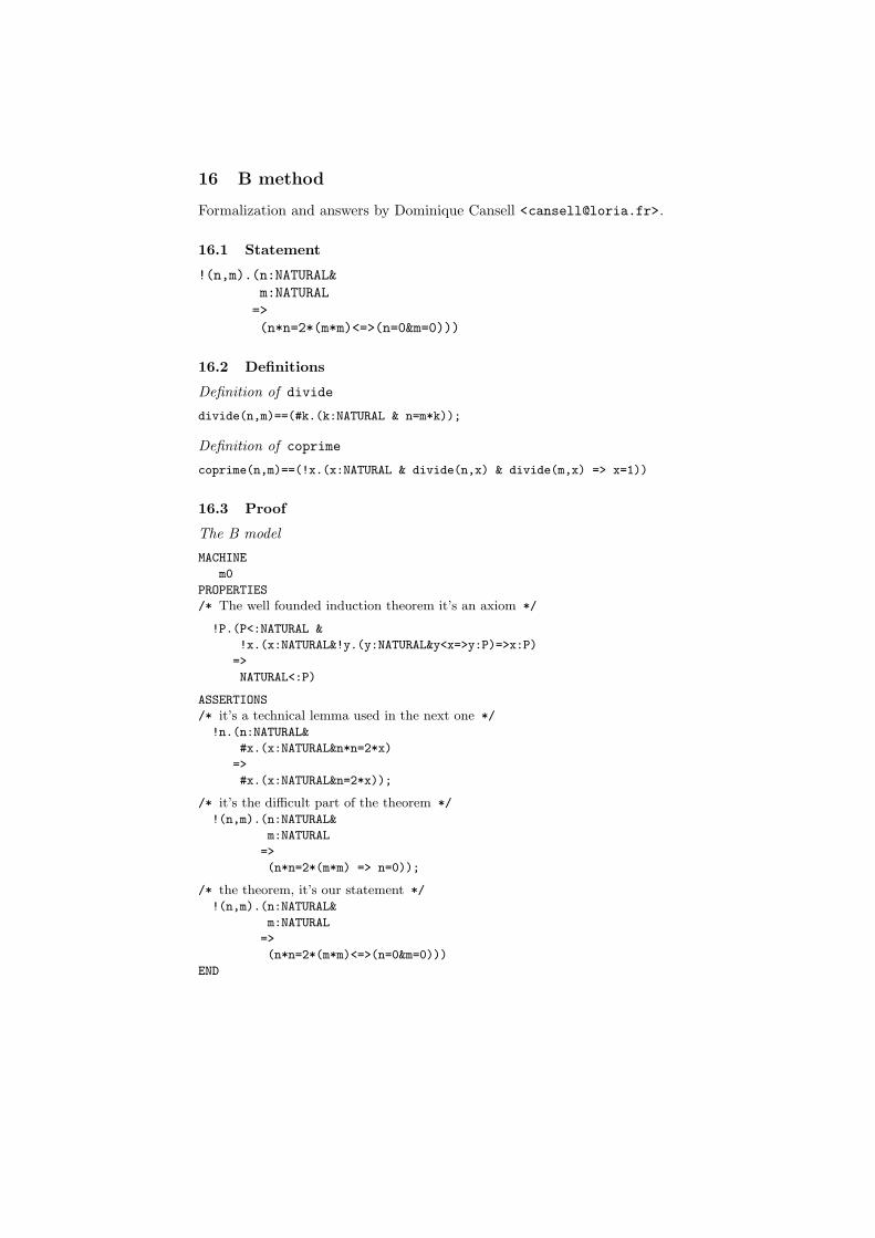
16 B method
Formalization and answers by Dominique Cansell <[email protected]>.
16.1 Statement
!(n,m).(n:NATURAL&
m:NATURAL
=>
(n*n=2*(m*m)<=>(n=0&m=0)))
16.2 Definitions
Definition of divide
divide(n,m)==(#k.(k:NATURAL & n=m*k));
Definition of coprime
coprime(n,m)==(!x.(x:NATURAL & divide(n,x) & divide(m,x) => x=1))
16.3 Proof
The B model
MACHINE
m0
PROPERTIES
/* The well founded induction theorem it’s an axiom */
!P.(P<:NATURAL &
!x.(x:NATURAL&!y.(y:NATURAL&y<x=>y:P)=>x:P)
=>
NATURAL<:P)
ASSERTIONS
/* it’s a technical lemma used in the next one */
!n.(n:NATURAL&
#x.(x:NATURAL&n*n=2*x)
=>
#x.(x:NATURAL&n=2*x));
/* it’s the difficult part of the theorem */
!(n,m).(n:NATURAL&
m:NATURAL
=>
(n*n=2*(m*m) => n=0));
/* the theorem, it’s our statement */
!(n,m).(n:NATURAL&
m:NATURAL
=>
(n*n=2*(m*m)<=>(n=0&m=0)))
END
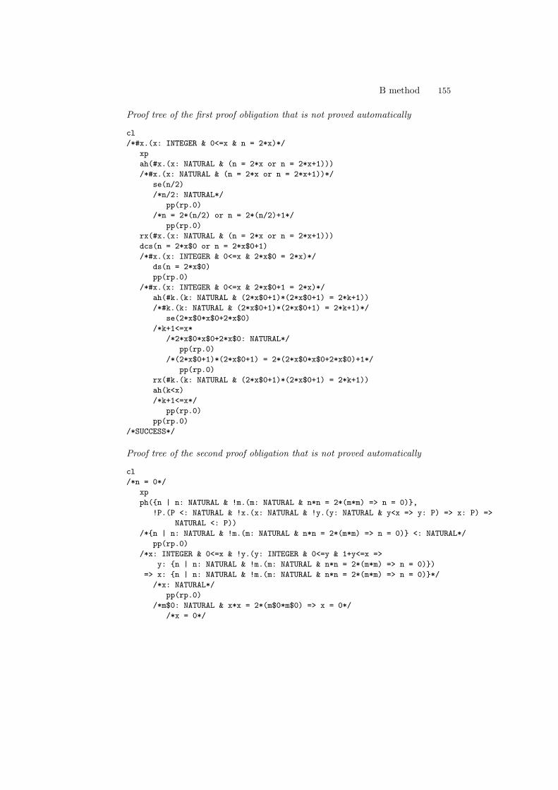
B method 155
Proof tree of the first proof obligation that is not proved automatically
cl
/*#x.(x: INTEGER & 0<=x & n = 2*x)*/
xp
ah(#x.(x: NATURAL & (n = 2*x or n = 2*x+1)))
/*#x.(x: NATURAL & (n = 2*x or n = 2*x+1))*/
se(n/2)
/*n/2: NATURAL*/
pp(rp.0)
/*n = 2*(n/2) or n = 2*(n/2)+1*/
pp(rp.0)
rx(#x.(x: NATURAL & (n = 2*x or n = 2*x+1)))
dcs(n = 2*x$0 or n = 2*x$0+1)
/*#x.(x: INTEGER & 0<=x & 2*x$0 = 2*x)*/
ds(n = 2*x$0)
pp(rp.0)
/*#x.(x: INTEGER & 0<=x & 2*x$0+1 = 2*x)*/
ah(#k.(k: NATURAL & (2*x$0+1)*(2*x$0+1) = 2*k+1))
/*#k.(k: NATURAL & (2*x$0+1)*(2*x$0+1) = 2*k+1)*/
se(2*x$0*x$0+2*x$0)
/*k+1<=x*
/*2*x$0*x$0+2*x$0: NATURAL*/
pp(rp.0)
/*(2*x$0+1)*(2*x$0+1) = 2*(2*x$0*x$0+2*x$0)+1*/
pp(rp.0)
rx(#k.(k: NATURAL & (2*x$0+1)*(2*x$0+1) = 2*k+1))
ah(k<x)
/*k+1<=x*/
pp(rp.0)
pp(rp.0)
/*SUCCESS*/
Proof tree of the second proof obligation that is not proved automatically
cl
/*n = 0*/
xp
ph(n | n: NATURAL & !m.(m: NATURAL & n*n = 2*(m*m) => n = 0),
!P.(P <: NATURAL & !x.(x: NATURAL & !y.(y: NATURAL & y<x => y: P) => x: P) =>
NATURAL <: P))
/*n | n: NATURAL & !m.(m: NATURAL & n*n = 2*(m*m) => n = 0) <: NATURAL*/
pp(rp.0)
/*x: INTEGER & 0<=x & !y.(y: INTEGER & 0<=y & 1+y<=x =>
y: n | n: NATURAL & !m.(m: NATURAL & n*n = 2*(m*m) => n = 0))
=> x: n | n: NATURAL & !m.(m: NATURAL & n*n = 2*(m*m) => n = 0)*/
/*x: NATURAL*/
pp(rp.0)
/*m$0: NATURAL & x*x = 2*(m$0*m$0) => x = 0*/
/*x = 0*/
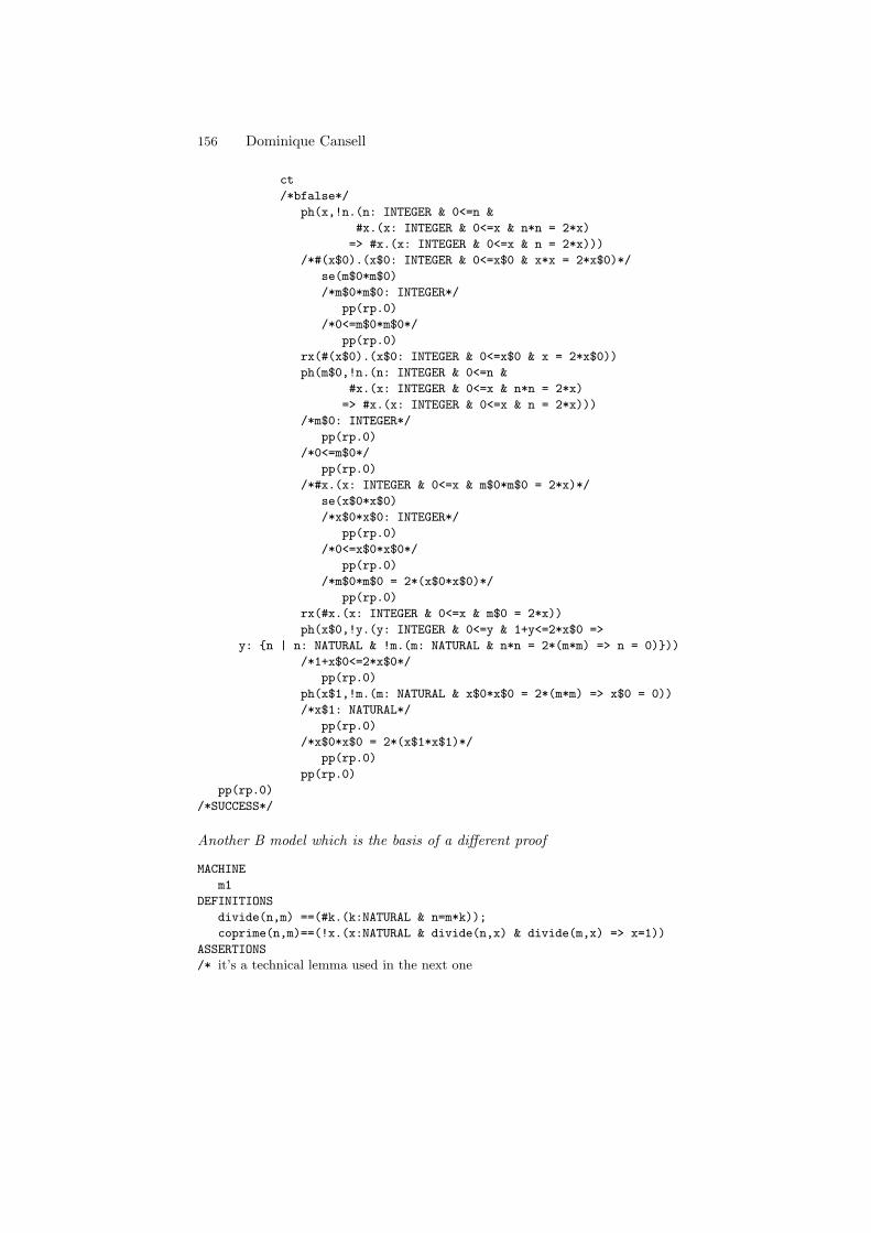
156 Dominique Cansell
ct
/*bfalse*/
ph(x,!n.(n: INTEGER & 0<=n &
#x.(x: INTEGER & 0<=x & n*n = 2*x)
=> #x.(x: INTEGER & 0<=x & n = 2*x)))
/*#(x$0).(x$0: INTEGER & 0<=x$0 & x*x = 2*x$0)*/
se(m$0*m$0)
/*m$0*m$0: INTEGER*/
pp(rp.0)
/*0<=m$0*m$0*/
pp(rp.0)
rx(#(x$0).(x$0: INTEGER & 0<=x$0 & x = 2*x$0))
ph(m$0,!n.(n: INTEGER & 0<=n &
#x.(x: INTEGER & 0<=x & n*n = 2*x)
=> #x.(x: INTEGER & 0<=x & n = 2*x)))
/*m$0: INTEGER*/
pp(rp.0)
/*0<=m$0*/
pp(rp.0)
/*#x.(x: INTEGER & 0<=x & m$0*m$0 = 2*x)*/
se(x$0*x$0)
/*x$0*x$0: INTEGER*/
pp(rp.0)
/*0<=x$0*x$0*/
pp(rp.0)
/*m$0*m$0 = 2*(x$0*x$0)*/
pp(rp.0)
rx(#x.(x: INTEGER & 0<=x & m$0 = 2*x))
ph(x$0,!y.(y: INTEGER & 0<=y & 1+y<=2*x$0 =>
y: n | n: NATURAL & !m.(m: NATURAL & n*n = 2*(m*m) => n = 0)))
/*1+x$0<=2*x$0*/
pp(rp.0)
ph(x$1,!m.(m: NATURAL & x$0*x$0 = 2*(m*m) => x$0 = 0))
/*x$1: NATURAL*/
pp(rp.0)
/*x$0*x$0 = 2*(x$1*x$1)*/
pp(rp.0)
pp(rp.0)
pp(rp.0)
/*SUCCESS*/
Another B model which is the basis of a different proof
MACHINE
m1
DEFINITIONS
divide(n,m) ==(#k.(k:NATURAL & n=m*k));
coprime(n,m)==(!x.(x:NATURAL & divide(n,x) & divide(m,x) => x=1))
ASSERTIONS
/* it’s a technical lemma used in the next one
B method 157
it’s the same as the previous one using divide */
!n.(n:NATURAL&
divide(n*n,2)
=>
divide(n,2));
/* The statement */
not(#(n,m).(n:NATURAL & m:NATURAL1 & n*n=2*(m*m) & coprime(n,m)))
END
16.4 System
What is the home page of the system?
<http://www-lsr.imag.fr/B/>
<http://www.b4free.com/>
<http://www.loria.fr/~cansell/cnp.html>
What are the books about the system?
J.-R. Abrial. The B Book - Assigning Programs to Meanings, CambridgeUniversity Press, 1996, ISBN 0-521-49619-5.
What is the logic of the system? First order logic and set theory. So we can havehigher order logic because we can quantify on all subset of a given set like forthe well founded induction theorem. Integers and Naturals are predefined.
What is the implementation architecture of the system? All tools of B4free arewritten in Logic-Solver. It is a language which looks like Prolog (inference rulesand rewrite rules with tactics). Click’n’Prove is written in xemacs. The xemacspart drives only B4free. Proofs are managed by B4free.
What does working with the system look like? The proof obligation generatorgenerates small proof obligations. Disjunction in hypotheses and conjunction ingoals are splitted.
A first automatic prover can be used to discharged proof obligation. This firstprover is rules based. To validate this prover a predicate prover was developed.This last prover is very powerful in set theory. It was added to the tool AtelierB and can be used for interactive proofs.
What is special about the system compared to other systems? With B we canprove theorems but we can also develop, using refinement, many models of a sys-tem. The proof accompany all the development. The proofs are invariant proofsand refinement proofs. We can add variables, invariants and events (which modifyvariables). Assertions are proved with properties (on constants) and invariants.
158 Dominique Cansell
What are other versions of the system? The proof presented here was createdusing the tools:
– B4free– Click’n’Prove
There are two other tools for the B method:
– Atelier B (ClearSy) <http://www.atelierb.societe.com/>B4free is an restricted version of Atelier B.
– B tool kit <http://www.b-core.com/btoolkit.html>
Who are the people behind the system? Jean-Raymond Abrial, ChristopheMetayer, Laurent Voisin and Dominique Cansell.
What are the main user communities of the system? Many industrials use (orhave used) the B method and associated tools like Atelier B: Gec-Alstom, Matra-Transport (now Siemens), RATP, Gemplus, Peugeot, . . .
B4free is now used by many researchers in formal method and refinementand used to teach the B method.
What large mathematical formalizations have been done in the system? Set the-ory until Zermelo theorem (every set can be well ordered with the choice axiom).
The most important is the development of systems like:
– embedded system of METEOR which is the success story– sequential and recursive progams– producer and consumer protocol: PCI– byte code verifier of the Java card– distributed algorithms: IEEE 1394 leader election protocol and spanning tree
detection– pointer programs: Schorr & Waite: a garbage collector, Michael & Scott: the
non blocking concurrent queue algorithm– large system: access control, a press– . . .
What needs to be explained about this specific proof?
The model. The B method is a modeling language developed by Jean-RaymondAbrial. One can model a (close) system starting from an abstract model andadding new details using refinement. Variables and events which transform vari-ables are defined in a model. Proofs (invariant and refinement) accompany allthe development. B4free is a free and limited (not provers) version of AtelierB. Atelier B is a commercial set of tools for the B method (typechecker, proofobligation generator, automatic and interactive provers). Atelier B was devel-oped and used to model the embedded system of METEOR (line 14 of Paris’ssubway).
B method 159
Click’n’Prove is a proactive interface for B4free especially for the interactiveprover.
For the “square root of two is not rational” challenge we have defined a modelwithout variables and events. We have only modeled, in set theory, the wellfounded induction theorem in the PROPERTIES clause and a list of assertions.Assertions can be proved only using properties (of constants) and the invariant(empty in our case). Properties correspond to axioms and assertions look liketheorems or lemmas (we can use the previous assertions to prove the next one).
In set theory we can define easily the well founded induction theorem withthis following property:
∀P ·
P ⊆ N ∧∀x · (x ∈ N ∧ ∀y · ( y ∈ N ∧ y < x ⇒ y ∈ P ) ⇒ x ∈ P )
⇒N ⊆ P
It’s our single axiom (we have already proved it in another development).Then we have define a first lemma which is used two times to prove the
difficult part of the theorem. This lemma express that if the square of a naturalnumber (here n) is even then the given natural number (n) is even too.
∀n ·
n ∈ N ∧∃x · (x ∈ N ∧ n × n = 2 × x)
⇒∃x · (x ∈ N ∧ n = 2 × x)
Then we can define the difficult part of the theorem which is the following
∀(n,m) · (n ∈ N ∧ m ∈ N ⇒ (n × n = 2 × m × m ⇒ n = 0))
We have proved this lemma using the well founded induction theorem. We haveinstantiated P with this following set:
n | n ∈ N ∧ ∀m · (m ∈ N ∧ n × n = 2 × (m × m) ⇒ n = 0)
Then after proving this lemma it’s very easy to prove the given theorem.
∀(n,m) · (n ∈ N ∧ m ∈ N) ⇒ (n × n = 2 × m × m ⇔ n = 0 ∧ m = 0)
In the system one then writes this B model in an ASCII form (! for ∀, # for ∃, <:for ⊆, . . .). This is the “B machine” which is shown at the start of Section 16.3on page 154.
Proof obligations. This machine provides five proof obligations (PO) because thelast assertion is splitted in three PO (n∗n = 2∗ (m∗m) ⇒ n = 0) which is thesecond assertion, (n∗n = 2∗(m∗m) ⇒ m = 0) and (n = 0 ∧ m = 0 ⇒ n∗n =2 ∗ (m ∗m)). Two of these tree PO (the first and the last one) are automaticallyproved by the B prover (force 0) and the second one is automatically proved bythe B prover (force 1). The other PO need some interactions.
160 Dominique Cansell
Proof. We explain the proofs with the three proof trees of the interactive proofs.These proof trees are provided automatically by the tool. [mk] and [zm] arebuttons which are very helpful to replay a script (all command between two[mk]) or to hide a part of the proof tree (button [zm] for zoom). After each [zm]
the current goal is displayed in a comment and after each [mk] an interactivecommand is displayed. Using Atelier B a user might type all the command butnow with the Click’n’Prove interface this command is displayed after one click(most often), a mouse selection (for a witness or a parameter) followed by aclick and sometimes type a parameter (using select & paste and/or using thekeyboard followed by a click. For a better explanation, please, see the demo onthis following web page <http://www.loria.fr/~cansell/demo.html>.
Next is the first proof tree. It finishes with SUCCESS. We have added somecomments to explain all interactions which are not provided by a single click.When pp(rp.0) (or pp(rp.1), pr) is displayed then the current goal is provedby an automatic prover. The two first commands cl (it’s a technical commandwhich can be removed) and xp (for expert mode, a beginner mode exists) areprovided automatically by the tool. dcs(a or b) launches a proof by case (casea then b)
[mk] cl
[zm] /*#x.(x: INTEGER & 0<=x & n = 2*x)*/
[mk] xp
[mk] ah(#x.(x: NATURAL & (n = 2*x or n = 2*x+1)))
It’s the first interaction; we have type the text inside ah(.) only. We have addedthis new hypothesis which expresses that n is odd or even.
We need to prove it.
[zm] /*#x.(x: NATURAL & (n = 2*x or n = 2*x+1))*/
[mk] se(n/2)
For our second interaction we have suggested n/2 as a witness for the existential.
[zm] /*n/2: NATURAL*/
[mk] pp(rp.0)
[zm] /*n = 2*(n/2) or n = 2*(n/2)+1*/
[mk] pp(rp.0)
[mk] rx(#x.(x: NATURAL & (n = 2*x or n = 2*x+1)))
[mk] dcs(n = 2*x$0 or n = 2*x$0+1)
[zm] /*#x.(x: INTEGER & 0<=x & 2*x$0 = 2*x)*/
[mk] pp(rp.0) /* if it’s not ok try ds(n = 2*x$0) before */
[zm] /*#x.(x: INTEGER & 0<=x & 2*x$0+1 = 2*x)*/
[mk] ah(#k.(k: NATURAL & (2*x$0+1)*(2*x$0+1) = 2*k+1))
It is our third interaction; we have added a new hypothesis. The square of(2*x$0+1) is odd. x$0 is a fresh variable which is provided by rx(#x.(x:
NATURAL & (n = 2*x or n = 2*x+1))) (remove existential).
[zm] /*#k.(k: NATURAL & (2*x$0+1)*(2*x$0+1) = 2*k+1)*/
[mk] se(2*x$0*x$0+2*x$0)
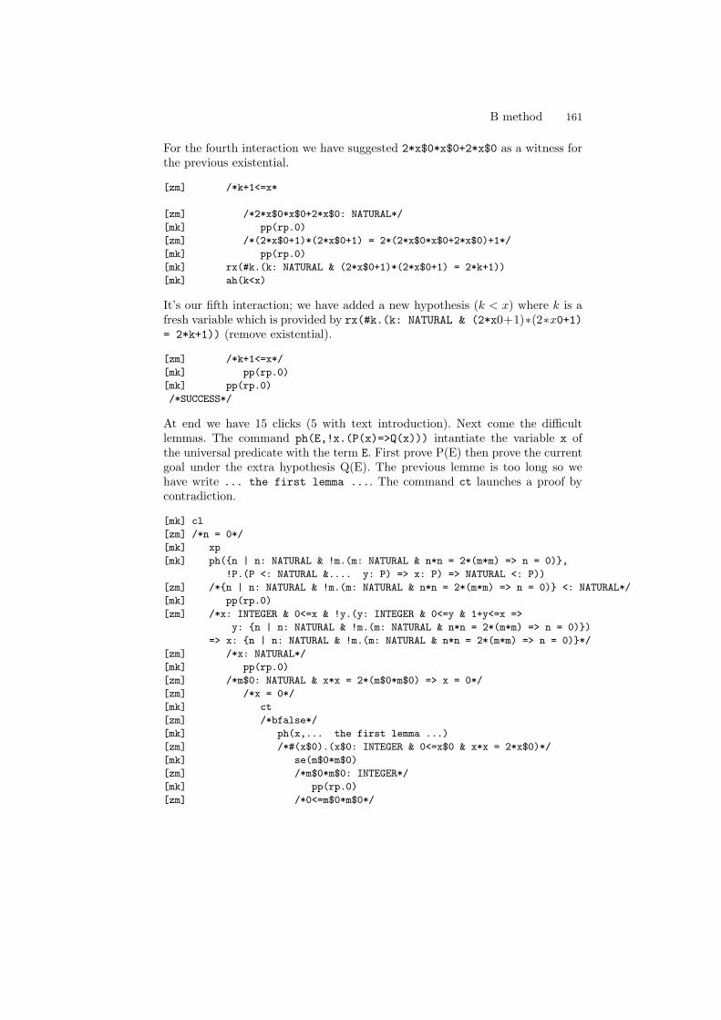
B method 161
For the fourth interaction we have suggested 2*x$0*x$0+2*x$0 as a witness forthe previous existential.
[zm] /*k+1<=x*
[zm] /*2*x$0*x$0+2*x$0: NATURAL*/
[mk] pp(rp.0)
[zm] /*(2*x$0+1)*(2*x$0+1) = 2*(2*x$0*x$0+2*x$0)+1*/
[mk] pp(rp.0)
[mk] rx(#k.(k: NATURAL & (2*x$0+1)*(2*x$0+1) = 2*k+1))
[mk] ah(k<x)
It’s our fifth interaction; we have added a new hypothesis (k < x) where k is afresh variable which is provided by rx(#k.(k: NATURAL & (2*x0+1)∗(2∗x0+1)= 2*k+1)) (remove existential).
[zm] /*k+1<=x*/
[mk] pp(rp.0)
[mk] pp(rp.0)
/*SUCCESS*/
At end we have 15 clicks (5 with text introduction). Next come the difficultlemmas. The command ph(E,!x.(P(x)=>Q(x))) intantiate the variable x ofthe universal predicate with the term E. First prove P(E) then prove the currentgoal under the extra hypothesis Q(E). The previous lemme is too long so wehave write ... the first lemma .... The command ct launches a proof bycontradiction.
[mk] cl
[zm] /*n = 0*/
[mk] xp
[mk] ph(n | n: NATURAL & !m.(m: NATURAL & n*n = 2*(m*m) => n = 0),
!P.(P <: NATURAL &.... y: P) => x: P) => NATURAL <: P))
[zm] /*n | n: NATURAL & !m.(m: NATURAL & n*n = 2*(m*m) => n = 0) <: NATURAL*/
[mk] pp(rp.0)
[zm] /*x: INTEGER & 0<=x & !y.(y: INTEGER & 0<=y & 1+y<=x =>
y: n | n: NATURAL & !m.(m: NATURAL & n*n = 2*(m*m) => n = 0))
=> x: n | n: NATURAL & !m.(m: NATURAL & n*n = 2*(m*m) => n = 0)*/
[zm] /*x: NATURAL*/
[mk] pp(rp.0)
[zm] /*m$0: NATURAL & x*x = 2*(m$0*m$0) => x = 0*/
[zm] /*x = 0*/
[mk] ct
[zm] /*bfalse*/
[mk] ph(x,... the first lemma ...)
[zm] /*#(x$0).(x$0: INTEGER & 0<=x$0 & x*x = 2*x$0)*/
[mk] se(m$0*m$0)
[zm] /*m$0*m$0: INTEGER*/
[mk] pp(rp.0)
[zm] /*0<=m$0*m$0*/
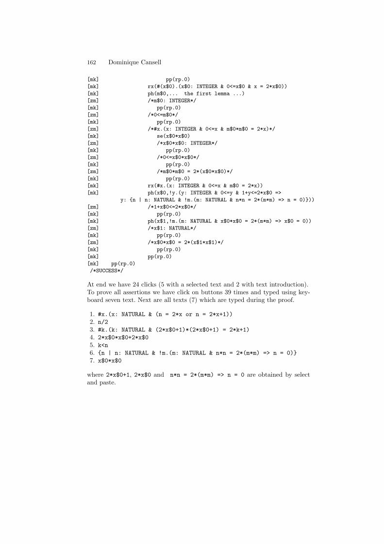
162 Dominique Cansell
[mk] pp(rp.0)
[mk] rx(#(x$0).(x$0: INTEGER & 0<=x$0 & x = 2*x$0))
[mk] ph(m$0,... the first lemma ...)
[zm] /*m$0: INTEGER*/
[mk] pp(rp.0)
[zm] /*0<=m$0*/
[mk] pp(rp.0)
[zm] /*#x.(x: INTEGER & 0<=x & m$0*m$0 = 2*x)*/
[mk] se(x$0*x$0)
[zm] /*x$0*x$0: INTEGER*/
[mk] pp(rp.0)
[zm] /*0<=x$0*x$0*/
[mk] pp(rp.0)
[zm] /*m$0*m$0 = 2*(x$0*x$0)*/
[mk] pp(rp.0)
[mk] rx(#x.(x: INTEGER & 0<=x & m$0 = 2*x))
[mk] ph(x$0,!y.(y: INTEGER & 0<=y & 1+y<=2*x$0 =>
y: n | n: NATURAL & !m.(m: NATURAL & n*n = 2*(m*m) => n = 0)))
[zm] /*1+x$0<=2*x$0*/
[mk] pp(rp.0)
[mk] ph(x$1,!m.(m: NATURAL & x$0*x$0 = 2*(m*m) => x$0 = 0))
[zm] /*x$1: NATURAL*/
[mk] pp(rp.0)
[zm] /*x$0*x$0 = 2*(x$1*x$1)*/
[mk] pp(rp.0)
[mk] pp(rp.0)
[mk] pp(rp.0)
/*SUCCESS*/
At end we have 24 clicks (5 with a selected text and 2 with text introduction).To prove all assertions we have click on buttons 39 times and typed using key-board seven text. Next are all texts (7) which are typed during the proof.
1. #x.(x: NATURAL & (n = 2*x or n = 2*x+1))
2. n/2
3. #k.(k: NATURAL & (2*x$0+1)*(2*x$0+1) = 2*k+1)
4. 2*x$0*x$0+2*x$0
5. k<n
6. n | n: NATURAL & !m.(m: NATURAL & n*n = 2*(m*m) => n = 0)
7. x$0*x$0
where 2*x$0+1, 2*x$0 and n*n = 2*(m*m) => n = 0 are obtained by selectand paste.
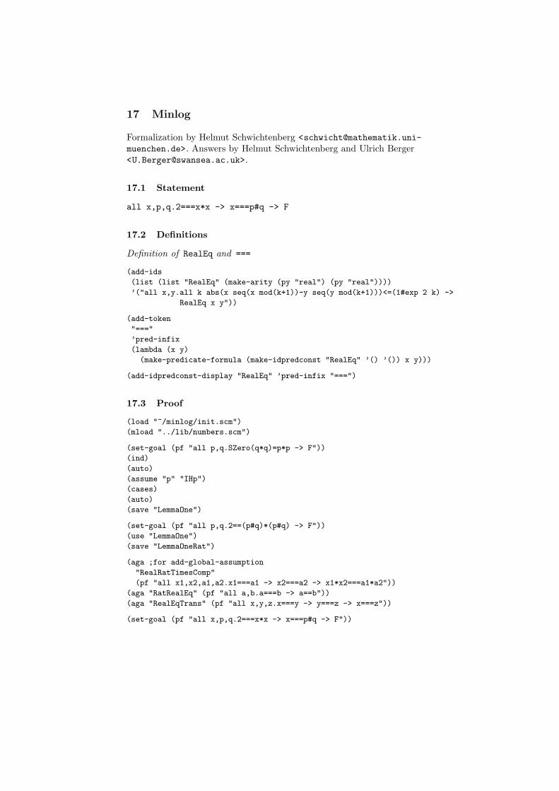
17 Minlog
Formalization by Helmut Schwichtenberg <[email protected]
muenchen.de>. Answers by Helmut Schwichtenberg and Ulrich Berger<[email protected]>.
17.1 Statement
all x,p,q.2===x*x -> x===p#q -> F
17.2 Definitions
Definition of RealEq and ===
(add-ids
(list (list "RealEq" (make-arity (py "real") (py "real"))))
’("all x,y.all k abs(x seq(x mod(k+1))-y seq(y mod(k+1)))<=(1#exp 2 k) ->
RealEq x y"))
(add-token
"==="
’pred-infix
(lambda (x y)
(make-predicate-formula (make-idpredconst "RealEq" ’() ’()) x y)))
(add-idpredconst-display "RealEq" ’pred-infix "===")
17.3 Proof
(load "~/minlog/init.scm")
(mload "../lib/numbers.scm")
(set-goal (pf "all p,q.SZero(q*q)=p*p -> F"))
(ind)
(auto)
(assume "p" "IHp")
(cases)
(auto)
(save "LemmaOne")
(set-goal (pf "all p,q.2==(p#q)*(p#q) -> F"))
(use "LemmaOne")
(save "LemmaOneRat")
(aga ;for add-global-assumption
"RealRatTimesComp"
(pf "all x1,x2,a1,a2.x1===a1 -> x2===a2 -> x1*x2===a1*a2"))
(aga "RatRealEq" (pf "all a,b.a===b -> a==b"))
(aga "RealEqTrans" (pf "all x,y,z.x===y -> y===z -> x===z"))
(set-goal (pf "all x,p,q.2===x*x -> x===p#q -> F"))
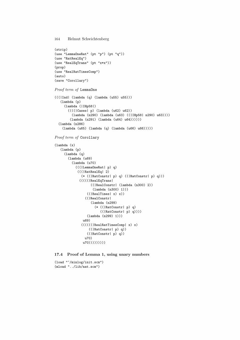
164 Helmut Schwichtenberg
(strip)
(use "LemmaOneRat" (pt "p") (pt "q"))
(use "RatRealEq")
(use "RealEqTrans" (pt "x*x"))
(prop)
(use "RealRatTimesComp")
(auto)
(save "Corollary")
Proof term of LemmaOne
(((|Ind| (lambda (q) (lambda (u55) u55)))
(lambda (p)
(lambda (|IHp58|)
((((|Cases| p) (lambda (u62) u62))
(lambda (n290) (lambda (u63) ((|IHp58| n290) u63))))
(lambda (n291) (lambda (u64) u64))))))
(lambda (n286)
(lambda (u65) (lambda (q) (lambda (u66) u66)))))
Proof term of Corollary
(lambda (x)
(lambda (p)
(lambda (q)
(lambda (u69)
(lambda (u70)
(((|LemmaOneRat| p) q)
(((|RatRealEq| 2)
(* ((|RatConstr| p) q) ((|RatConstr| p) q)))
(((((|RealEqTrans|
((|RealConstr| (lambda (n300) 2))
(lambda (n300) 1)))
((|RealTimes| x) x))
((|RealConstr|
(lambda (n299)
(* ((|RatConstr| p) q)
((|RatConstr| p) q))))
(lambda (n299) 1)))
u69)
((((((|RealRatTimesComp| x) x)
((|RatConstr| p) q))
((|RatConstr| p) q))
u70)
u70)))))))))
17.4 Proof of Lemma 1, using unary numbers
(load "~/minlog/init.scm")
(mload "../lib/nat.scm")
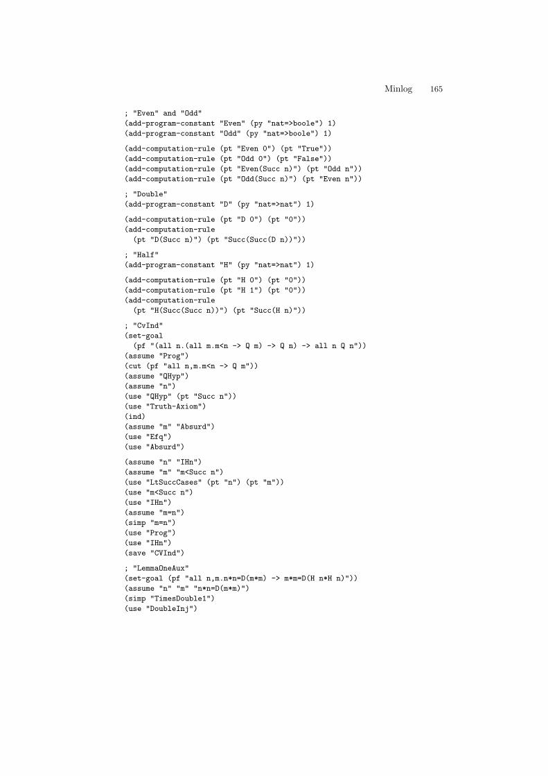
Minlog 165
; "Even" and "Odd"
(add-program-constant "Even" (py "nat=>boole") 1)
(add-program-constant "Odd" (py "nat=>boole") 1)
(add-computation-rule (pt "Even 0") (pt "True"))
(add-computation-rule (pt "Odd 0") (pt "False"))
(add-computation-rule (pt "Even(Succ n)") (pt "Odd n"))
(add-computation-rule (pt "Odd(Succ n)") (pt "Even n"))
; "Double"
(add-program-constant "D" (py "nat=>nat") 1)
(add-computation-rule (pt "D 0") (pt "0"))
(add-computation-rule
(pt "D(Succ n)") (pt "Succ(Succ(D n))"))
; "Half"
(add-program-constant "H" (py "nat=>nat") 1)
(add-computation-rule (pt "H 0") (pt "0"))
(add-computation-rule (pt "H 1") (pt "0"))
(add-computation-rule
(pt "H(Succ(Succ n))") (pt "Succ(H n)"))
; "CvInd"
(set-goal
(pf "(all n.(all m.m<n -> Q m) -> Q n) -> all n Q n"))
(assume "Prog")
(cut (pf "all n,m.m<n -> Q m"))
(assume "QHyp")
(assume "n")
(use "QHyp" (pt "Succ n"))
(use "Truth-Axiom")
(ind)
(assume "m" "Absurd")
(use "Efq")
(use "Absurd")
(assume "n" "IHn")
(assume "m" "m<Succ n")
(use "LtSuccCases" (pt "n") (pt "m"))
(use "m<Succ n")
(use "IHn")
(assume "m=n")
(simp "m=n")
(use "Prog")
(use "IHn")
(save "CVInd")
; "LemmaOneAux"
(set-goal (pf "all n,m.n*n=D(m*m) -> m*m=D(H n*H n)"))
(assume "n" "m" "n*n=D(m*m)")
(simp "TimesDouble1")
(use "DoubleInj")
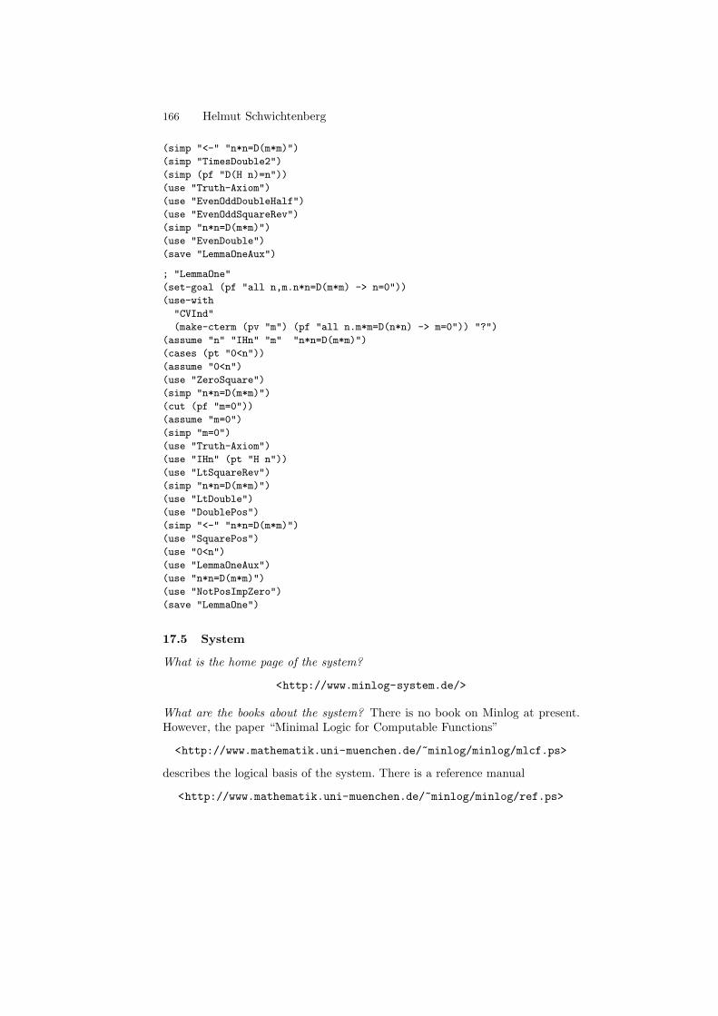
166 Helmut Schwichtenberg
(simp "<-" "n*n=D(m*m)")
(simp "TimesDouble2")
(simp (pf "D(H n)=n"))
(use "Truth-Axiom")
(use "EvenOddDoubleHalf")
(use "EvenOddSquareRev")
(simp "n*n=D(m*m)")
(use "EvenDouble")
(save "LemmaOneAux")
; "LemmaOne"
(set-goal (pf "all n,m.n*n=D(m*m) -> n=0"))
(use-with
"CVInd"
(make-cterm (pv "m") (pf "all n.m*m=D(n*n) -> m=0")) "?")
(assume "n" "IHn" "m" "n*n=D(m*m)")
(cases (pt "0<n"))
(assume "0<n")
(use "ZeroSquare")
(simp "n*n=D(m*m)")
(cut (pf "m=0"))
(assume "m=0")
(simp "m=0")
(use "Truth-Axiom")
(use "IHn" (pt "H n"))
(use "LtSquareRev")
(simp "n*n=D(m*m)")
(use "LtDouble")
(use "DoublePos")
(simp "<-" "n*n=D(m*m)")
(use "SquarePos")
(use "0<n")
(use "LemmaOneAux")
(use "n*n=D(m*m)")
(use "NotPosImpZero")
(save "LemmaOne")
17.5 System
What is the home page of the system?
<http://www.minlog-system.de/>
What are the books about the system? There is no book on Minlog at present.However, the paper “Minimal Logic for Computable Functions”
<http://www.mathematik.uni-muenchen.de/~minlog/minlog/mlcf.ps>
describes the logical basis of the system. There is a reference manual
<http://www.mathematik.uni-muenchen.de/~minlog/minlog/ref.ps>
Minlog 167
and a tutorial (by Laura Crosilla)
<http://www.mathematik.uni-muenchen.de/~minlog/minlog/tutor.ps>
What is the logic of the system? Minimal logic, hence (via ex-falso-quodlibetand stability axioms) also intuitionistic and classical logic are included. Quan-tification over higher order functionals (of any finite type) is possible. There arealso (parametric) type variables and predicate variables, but they are seen asplace-holders for concrete types and comprehension terms, i.e., they are (im-plicitly) universally quantified (this is sometimes called ML-polymorphism). Tokeep the system predicative and moreover proof-theoretically weak (i.e., conser-vative over Heyting arithmetic), quantification over type and predicate variablesis not allowed. Inductive data types and inductive definitions with their usualintroduction and elimination rules are present. Of course, the latter in generalincreases the proof-theoretic strength.
What is the implementation architecture of the system? The system is writ-ten in Scheme (a Lisp dialect). Types, terms, formulas and proofs are separateentities. Terms and (following the Curry-Howard correspondence) also proofs areseen as λ-terms. There is a simple proof checking algorithm, which guaranteesthe correctness of a generated proof object.
What does working with the system look like? The standard LCF tactic styleis used. David Aspinall’s “Proof General” interface has also been adapted (byStefan Schimanski).
What is special about the system compared to other systems? The intended modelconsists of the partial continuous functionals (in the Scott-Ersov sense), so par-tiality is built in from the outset. Program extraction can be done from con-structive as well as from classical proofs; the latter uses a refined form of HarveyFriedman’s A-translation. A proof that an extracted program realizes its speci-fication can be machine generated.
Function (or better: program) constants (again of any finite type) have user-defined computation and rewrite rules associated with them. Using Scheme’sevaluation, terms are normalized (“normalization by evaluation”) w.r.t. all stan-dard conversion rules (β, η, recursion, user-defined computation and rewriterules), and terms with the same normal form are identified. This feature canshorten proofs drastically, as seen in the example above. Rewrite rules are tobe viewed as part of the proof object, but, in the current version of Minlog,are not kept as part of the proof term. The system supports working in proof-theoretically weak theories, in order to have control over the complexity of ex-tracted programs (this is work in progress).
What are other versions of the system? There is only one supported version.The current one is 4.0.
Who are the people behind the system? The Munich (LMU) logic group, and theSwansea logic group.
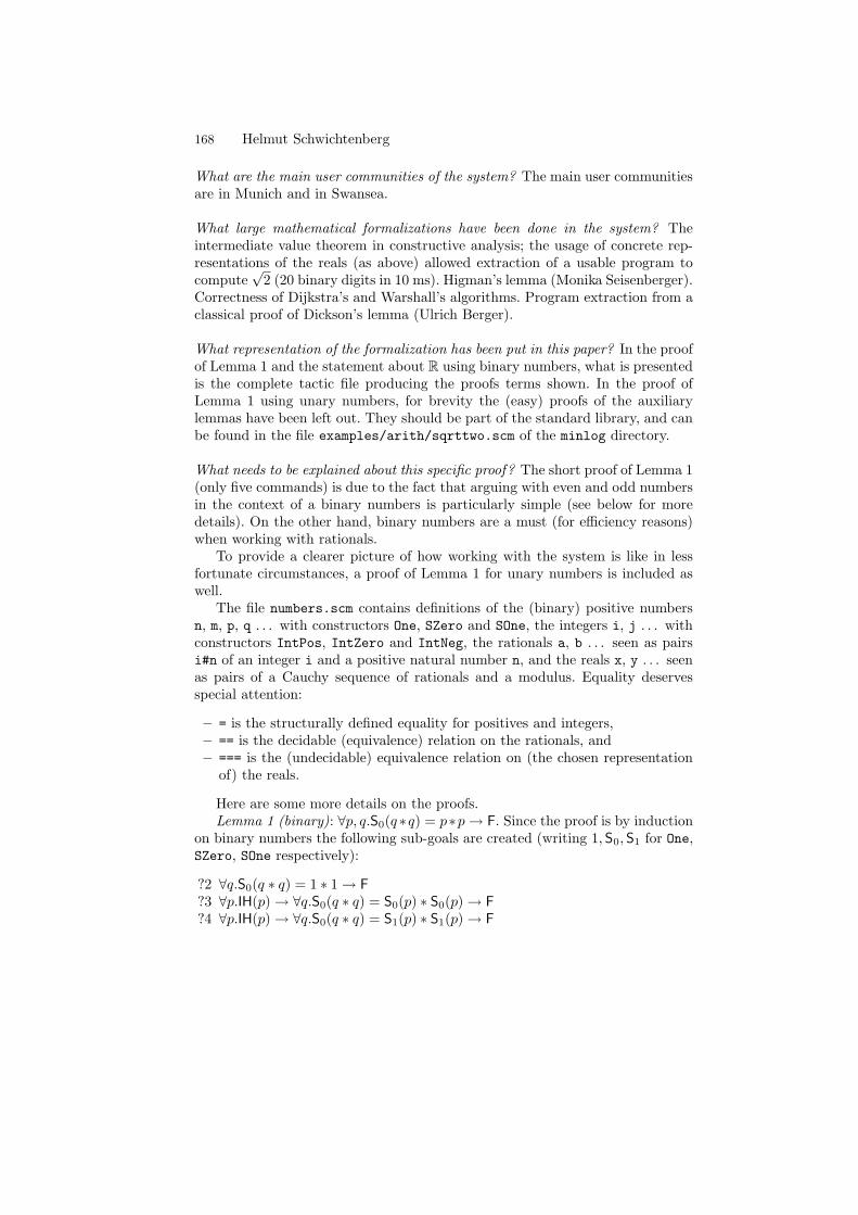
168 Helmut Schwichtenberg
What are the main user communities of the system? The main user communitiesare in Munich and in Swansea.
What large mathematical formalizations have been done in the system? Theintermediate value theorem in constructive analysis; the usage of concrete rep-resentations of the reals (as above) allowed extraction of a usable program tocompute
√2 (20 binary digits in 10 ms). Higman’s lemma (Monika Seisenberger).
Correctness of Dijkstra’s and Warshall’s algorithms. Program extraction from aclassical proof of Dickson’s lemma (Ulrich Berger).
What representation of the formalization has been put in this paper? In the proofof Lemma 1 and the statement about R using binary numbers, what is presentedis the complete tactic file producing the proofs terms shown. In the proof ofLemma 1 using unary numbers, for brevity the (easy) proofs of the auxiliarylemmas have been left out. They should be part of the standard library, and canbe found in the file examples/arith/sqrttwo.scm of the minlog directory.
What needs to be explained about this specific proof? The short proof of Lemma 1(only five commands) is due to the fact that arguing with even and odd numbersin the context of a binary numbers is particularly simple (see below for moredetails). On the other hand, binary numbers are a must (for efficiency reasons)when working with rationals.
To provide a clearer picture of how working with the system is like in lessfortunate circumstances, a proof of Lemma 1 for unary numbers is included aswell.
The file numbers.scm contains definitions of the (binary) positive numbersn, m, p, q . . . with constructors One, SZero and SOne, the integers i, j . . . withconstructors IntPos, IntZero and IntNeg, the rationals a, b . . . seen as pairsi#n of an integer i and a positive natural number n, and the reals x, y . . . seenas pairs of a Cauchy sequence of rationals and a modulus. Equality deservesspecial attention:
– = is the structurally defined equality for positives and integers,– == is the decidable (equivalence) relation on the rationals, and– === is the (undecidable) equivalence relation on (the chosen representation
of) the reals.
Here are some more details on the proofs.Lemma 1 (binary): ∀p, q.S0(q ∗q) = p∗p → F. Since the proof is by induction
on binary numbers the following sub-goals are created (writing 1,S0,S1 for One,SZero, SOne respectively):
?2 ∀q.S0(q ∗ q) = 1 ∗ 1 → F
?3 ∀p.IH(p) → ∀q.S0(q ∗ q) = S0(p) ∗ S0(p) → F
?4 ∀p.IH(p) → ∀q.S0(q ∗ q) = S1(p) ∗ S1(p) → F
Minlog 169
where IH(p) ≡ ∀q.S0(q ∗ q) = p ∗ p → F.Goal ?2 is solved by normalizing 1 ∗ 1 to 1 and hence S0(q ∗ q) = 1 ∗ 1
to F. Similarly, in goal ?4 the premise S0(q ∗ q) = S1(p) ∗ S1(p) normalizesto F since S1(p) ∗ S1(p) normalizes to a term of the form S1( ). The premiseS0(q ∗ q) = S0(p) ∗ S0(p) of goal ?3 normalizes to q ∗ q = S0(p ∗ p). Consider thepossible forms of q: 1, S0(r), or S1(r). In the first and last case q∗q normalizes toa term of the form S1( ) hence the equation normalizes to F. In the second casethe equation normalizes to S0(q ∗ q) = p ∗ p which implies F by the inductionhypothesis. The system does all this fully automatically, except for the caseanalysis on q.
Lemma 1 Rat : ∀p, q.2 == p
q∗ p
q→ F. Up to normalization this is identical to
Lemma 1, since 2 == p
q∗ p
qnormalizes to S0(q ∗ q) = p ∗ p.
Global assumption on equalities on the rationals and the reals. Here the factis used that the rationals are coerced into the reals.
Lemma 1 (unary). The 12th command, (use "IHn" (pt "H n")), reducesthe goal m = 0 with the help of the induction hypothesis ∀m.m < n → ∀k.m ∗m = D(k ∗ k) → m = 0. The argument (pt "H n") is not –as one might think–used to instantiate the first universal quantifier, ∀m, but the second one, ∀k,which is the only quantifier left uninstantiated after matching the goal with thehead of the induction hypothesis.