the science of dbms: query optimization
TRANSCRIPT

(c) 2015 Independent SAP Technical User GroupAnnual Conference, 2015
- ISUG TECH 2015- ISUG TECH 2015ConferenceConference
: The Science of DBMS Query Optimization : The Science of DBMS Query Optimization , Jeff Tallman SAP ASE Product Management , Jeff Tallman SAP ASE Product Management

2Annual Conference, 2015 (c) 2015 Independent SAP Technical User Group
AgendaAgendaIntro & Optimization Basics
q Basic optimization cost factorsq Procedure Cache (ASE)
Query Processing & Optimizationq Internals of QPq Impact of LOP-treeq Understanding optimization vs. execution
Optimization Costingq Histograms & column densitiesq IN() & OR clausesq Out of range histogramsq Joins & Multi-column densities
Controlling optimizationq Sp_chgattribute ‘opt concurrency threshold’q Sp_modifystatsq Resource Granularity

3Annual Conference, 2015 (c) 2015 Independent SAP Technical User Group
Some CaveatsSome CaveatsQuery Optimization is very vendor proprietary/confidential
q You can buy books on generic optimization techniques….q …but DBMS vendors hire PhD’s to develop implementations
ü Query performance often depends on how good the optimization is
ü This is a key difference between OpenSource and COTS DBMS packages
The strength of the query optimizer is largely due to the $$$ vested in skills of highly educated staffing
As a result, this session will NOT explain the secrets of ASE’s optimizerq However, it will explain how it works, what influences it, what
resources it uses, etc.q Additionally, most modern optimizers all use the same lava
tree modelü Query optimization is based on an upside down tree with
data spewing out the top

4Annual Conference, 2015 (c) 2015 Independent SAP Technical User Group
Goal of This SessionGoal of This SessionThe goal of this session
q Help you understand the intricacies of query optimization
q Use that knowledge to write queries that can be optimized better
q Understand how/when additional index statistics might be necessary
q Understand how to influence optimizationü Other than the usual index forcing, AQP plan clauses,
etc.q Differentiate when the optimizer is messing up…or your
SQL didAssumptions for this session
q You understand optimization basics (histograms, selectivity, etc.)
q You understand basic optimization diagnostics (set option show)ü Not so much the output as the fact the commands
exist

5Annual Conference, 2015 (c) 2015 Independent SAP Technical User Group
Rules Based OptimizationRules Based OptimizationRules based optimization
q Index selection and join order processing are based on specific rules
q For example:ü Index selection is based on the index whose leading columns
are most covered by query predicatesü Join order is based on left to right ordering in FROM clause
designates driving tables/join orderThe good, bad & ugly
q Very good for extremely volatile data in which histogram statistics are often stale/impossible
q Good for insert intensive monotonic sequences in which new values are out of range of histograms
q Not so good…in fact sometimes ugly…on data that has any sort of skew with highly repetitive values
q The really ugly part is if the SQL coders don’t know the “rules”

6Annual Conference, 2015 (c) 2015 Independent SAP Technical User Group
Cost Based OptimizationCost Based OptimizationUsed by all mainstream DBMS’s
q Oracle, IBM DB2 UDB, MS SQL, ASEAttempts to find the cheapest method to perform query
q Uses some factoring of IO, CPU and memoryq Formula for cost varies among DBMS’s
The key to costing is index/column histogramsq In a sense, histograms attempt to report the relative skew of
the data being queriedq The optimizer’s goal is to find the cheapest access path
considering the data skewq If it wasn’t for the histogram reporting the skew…a rules
based optimization would be the only choice

7Annual Conference, 2015 (c) 2015 Independent SAP Technical User Group
Simple Cost Factors (1)Simple Cost Factors (1)Physical IO
q This is pretty obvious – disks are slow.q But we also need to predict how many writes (and then
re-reads) we may need to do for intermediate resultsLogical IO
q This is where PhD’s are madeq Remember, at query optimization time, we don’t know
what pages we are after….q However, we need to determine how many LIOs we
expect based onü How much of a table is already in cacheü How often we may revisit the same pages for multiple
rows

8Annual Conference, 2015 (c) 2015 Independent SAP Technical User Group
Simple Cost Factors (2)Simple Cost Factors (2)Memory
q Besides LIO, memory can be used to cache query intermediate results such as subquery results, hash tables for HJ, etc.
q In addition, memory can be used to avoid writes – e.g. in memory sorts for order by, sort merge joins, etc.
CPUq Again, fairly basic – but every LIO requires CPU
ü We need to do the data comparison for non-index key predicates
ü Again, though, we really don’t know how fast the CPU is that we are on…and how awful the data comparisons will be
We might apply some fuzzy logic on LIKE ‘%pattern%’ on large varchars or something….but …..
q Also, basic – sorts require CPU as wellü Distinct processing, Order by processing, etc.

9Annual Conference, 2015 (c) 2015 Independent SAP Technical User Group
Procedure Cache & OptimizationProcedure Cache & OptimizationOptimization • one of the consumers of proc cache
q Index statistics are loaded into proc cache for each query optimizationü Visible with set option show long
q Temporary work plans are created in proc cacheq Reported via set statistics resource onq Total consumption not a lot (rule of thumb = #engines * 2MB for OLTP)
Two big problemsq There is no ‘sharing’ of index statistics in proc cacheq Index statistics don’t stay in cache
ü As soon as query optimization for that query is finished, the proc buffers are deallocated.
ü This means a TON of logical IOs on sysstatistics Unless you use a lot of fully prepared statements or stored procedures
ü Hence you really want to ensure you have a dedicated systables cache
q This is largely due to historical aspectsü Remember, in 1984, 1MB of memory was a lotü Today, sum of the index statistics are likely 256MB or less

10Annual Conference, 2015 (c) 2015 Independent SAP Technical User Group
Loading Stats & Proc Cache UsageLoading Stats & Proc Cache UsageCreating Initial Statistics for table aqi_locations l .....Done creating Initial Statistics for table aqi_locations l
Creating Initial Statistics for table aqi_samples s .....Done creating Initial Statistics for table aqi_samples s
Creating Initial Statistics for index aqi_locations_PK .....Done creating Initial Statistics for index aqi_locations_PK
…Phase 2b initialization of OptBlock0 ...
... phase 2b done.Start merging statistics for table aqi_locations l ..... Done merging statistics for table aqi_locations l Start merging statistics for table aqi_samples s ..... Done merging statistics for table aqi_samples s
…
Total estimated I/O cost for statement 1 (at line 1): 33926.
Parse and Compile Time 0.Adaptive Server cpu time: 0 ms.Statement: 1 Compile time resource usage: (est worker processes=0 proccache=126),
Execution time resource usage: (worker processes=0 auxsdesc=0 plansize=14 proccache=23 proccache hwm=28 tempdb hwm=2)
Private buffer count: 48,Private HWM buffer count: 48
use demo_dbgoset statement_cache offset switch on 3604set option show longset statistics time, io, resource, plancost onset showplan ongoselect l.city, l.county, s.sample_date, s.air_tempfrom aqi_locations l, aqi_samples swhere l.location_id=s.location_id and s.sample_date = 'July 1 2000 12:00:00:000PM' and l.state='PA' and s.weather='Overcast' and s.air_temp = 90goset switch off 3604set option show offset statistics time, io, resource, plancost offset showplan offgo
Loading stats
Compile time proc cache usage for stats & work plans
126 proc pages * 2k memory page = 252KB

(c) 2015 Independent SAP Technical User GroupAnnual Conference, 2015
QUERY PROCESSING & QUERY PROCESSING & OPTIMIZATIONOPTIMIZATION
Internals, LOP Trees & Execution

12Annual Conference, 2015 (c) 2015 Independent SAP Technical User Group
QP PhasesQP PhasesReceive bufferSQL ParsingQuery Normalization
q Resolves object id’sq Replaces system
functions/functions with literals with literal values
q Rearranges AND/OR according to precedence
Pre-Processingq Transforms subqueriesq Rearranges aggregatesq Creates Logical Operators
(LOP)Query OptimizationQuery Execution
TDSLANG ƒ select * from table where due_dt =getdate() and recv_date is null
SELECT � {column list}FROM � table COND1 � due_dt <=getdate()COND2 (AND) r recv_date is null
SELECT � {column id’s & datatypes}FROM � objid=123456COND1 � col_id=3 (dt) >= (dt) ‘Jan 1 2015’COND2 (AND) � col_id=4 (dt) IS NULL
Receive Buffer
SQL Parsing
Normalization
Pre-Processing
Query Optimization
Query Execution
Focus

13Annual Conference, 2015 (c) 2015 Independent SAP Technical User Group
Some Notes on WaitEventsSome Notes on WaitEventsBelieve it or not….
q Until execution phase, all the rest counts as ‘awaiting command’ in sp_who or WaitEvent ID=250 in monProcessWaits
q It kinda makes sense….until query is executing…it isn’t executing…
q ….but parsing, compiling & optimization all can use considerable CPU timeü Sooo…that is why set statistics time on reports
compile time separatelySooo…if ‘awaiting command’ a lot….
q See if packets received are increasingq Switch to fully prepared statements or procs via RPC
calls

14Annual Conference, 2015 (c) 2015 Independent SAP Technical User Group
Optimization Starts with LOP TreeOptimization Starts with LOP TreeDuring pre-processing phase, a LOP tree is created
q A high level tree that represents the logical operations representing the relations between the entities
q Often, the LOP tree is the first place where optimization starts to go wrong….due to bad query formation by developers
Use ‘set option show on’ to see lop treeq It will be near the very top of the outputq You will need trace 3604 enabled
During execution, a physical operator (Pop) is usedq Lop � Joinq Pop � NLJoin

15Annual Conference, 2015 (c) 2015 Independent SAP Technical User Group
Example QueryExample Queryuse demo_dbgoset option show onset switch on 3604set statistics plancost, time, resource, io onset showplan onset statement_cache off -- avoid rerunning goofy plans from previous runset nodata on -- don’t return results (avoids network time/scrolling of large results)goselect l.county, avg(s.air_temp) from aqi_locations l, aqi_samples s where l.location_id=s.location_id and s.sample_date between 'July 1 2000 00:01am' and 'July 31 2000 23:59:59' and state='PA' group by l.countygoset option show offset switch off 3604set statistics plancost, time, resource, io offset showplan off--set statement_cache offgo

16Annual Conference, 2015 (c) 2015 Independent SAP Technical User Group
Example LOP TreeExample LOP Tree1> select l.county, avg(s.air_temp)2> from aqi_locations l,3> aqi_samples s4> where l.location_id=s.location_id5> and s.sample_date between 'July 1 2000 00:01am' and 'July 31 2000 23:59:59'6> and state='PA'7> group by l.countyThe Lop tree:( project
( group( join
( scan aqi_locations)
( scan aqi_samples)
)
)
)

17Annual Conference, 2015 (c) 2015 Independent SAP Technical User Group
LOP Tree & OptBlocksLOP Tree & OptBlocksEach LOP tree level becomes an Optblock
q Outermost block (0) is one below (project)
q Each block will generally have a relational operator
ü Join, group, scalar, etc.ü Scan is only considered an
operator if the query only has one entity and no other operators
Optimizer will determine an optimal plan for that block
q ASE set option show will print optimization for each optblock
q The optblock list is also printed at the top
The Lop tree:( project
( group( join
( scan aqi_locations)
( scan aqi_samples)
)
)
)
OptBlock1OptBlock0

18Annual Conference, 2015 (c) 2015 Independent SAP Technical User Group
Example OptBlockExample OptBlockThe Lop tree:…
OptBlock1 The Lop tree:( join
( scan aqi_locations)( scan aqi_samples)
)Generic Tables: ( Gtt1( aqi_locations l ) Gtt2( aqi_samples s ) Gti3( aqi_locations_PK ) …Generic Columns: ( Gc0(aqi_locations l ,Rid) Gc1(aqi_locations l ,state) Gc2(aqi_locations l ,location_id) …Predicates: ( { aqi_samples s.sample_date} >= "Jul 1 2000 12:01AM" tc:{5} …Transitive Closures: ( Tc0 = { Gc0(aqi_locations l ,Rid)} …
OptBlock0 The Lop tree:( pseudoscan)Generic Tables: ( Gtg0 ) Generic Columns: ( Gc8(Gtg0 ,_gcelement_8) Gc9(Gtg0 ,_gcelement_9) Gc10(Gtg0 ,_gcelement_10) … Predicates: ( ) Transitive Closures: ( Tc7 = { Gc8(Gtg0 ,_gcelement_8) Gc12(Gtg0 ,_virtualagg) …

19Annual Conference, 2015 (c) 2015 Independent SAP Technical User Group
I f you have any doubtsI f you have any doubtsI f your index is being considered….
q It will be listed in Generic Tables with Gttiü Format is <tablelist>, <indexlist>
q Example:ü Generic Tables: ( Gtt1( aqi_locations l ) Gtt2( aqi_samples
s ) Gti3( aqi_locations_PK ) Gti4( city_state_idx ) Gti5( county_state_idx ) Gti6( aqi_samples_PK ) Gti7( aqi_weather_date_idx ) )
I f your where clause is being considered…q It will be listed in Predicatesq Example:
ü Predicates: ( { aqi_samples s.sample_date} >= "Jul 1 2000 12:01AM" tc:{5} { aqi_samples s.sample_date} <= "Jul 31 2000 11:59PM" tc:{5} { aqi_locations l.state} = 'PA' tc:{1} )

20Annual Conference, 2015 (c) 2015 Independent SAP Technical User Group
To find optimization detailsTo find optimization detailsLook for optblock begin/end section markers in output
q Begin **************************************************************************
**** BEGIN: Search Space Traversal for OptBlock1 **************************************************************************
****
q End **************************************************************************
**** DONE: Search Space Traversal for OptBlock1 **************************************************************************
****
Any section could be fairly lengthyq The key is to find the optblock where you think the
problem is….

21Annual Conference, 2015 (c) 2015 Independent SAP Technical User Group
The LOP role …a tale of two queriesThe LOP role …a tale of two queries
select * into tempdb..my_objects from sybsystemprocs..sysobjects
create index type_date_idx on tempdb..my_objects (type, crdate)
declare @type char(2)select @type='P'select @type, max(crdate)from tempdb..my_objectswhere type=@type
declare @type char(2)select @type='P'select type, max(crdate)from tempdb..my_objectswhere type=@typegroup by type
The setup: “Good” Query: “Bad” Query:

22Annual Conference, 2015 (c) 2015 Independent SAP Technical User Group
The showplans…and final IO costsThe showplans…and final IO costsQUERY PLAN FOR STATEMENT 2 (at line 9).Optimized using Serial Mode
STEP 1 The type of query is SELECT.
2 operator(s) under root
|ROOT:EMIT Operator (VA = 2) | | |SCALAR AGGREGATE Operator (VA = 1) | | Evaluate Ungrouped MAXIMUM AGGREGATE. | | Scanning only up to the first qualifying row. | | | | |SCAN Operator (VA = 0) | | | FROM TABLE | | | my_objects | | | Index : type_date_idx | | | Backward scan. | | | Positioning by key. | | | Index contains all needed columns. Base table will not be read. | | | Keys are: | | | type ASC | | | Using I/O Size 4 Kbytes for index leaf pages. | | | With LRU Buffer Replacement Strategy for index leaf pages.
Total estimated I/O cost for statement 2 (at line 9): 54.…Table: my_objects scan count 1, logical reads: (regular=2 apf=0 total=2),
physical reads: (regular=0 apf=0 total=0), apf IOs used=0Total actual I/O cost for this command: 4.
“Good” Query Plan & Cost:QUERY PLAN FOR STATEMENT 2 (at line 9).Optimized using Serial Mode
STEP 1 The type of query is SELECT.
3 operator(s) under root
|ROOT:EMIT Operator (VA = 3) | | |RESTRICT Operator (VA = 2)(0)(0)(0)(4)(0) | | | | |GROUP SORTED Operator (VA = 1) | | | Evaluate Grouped MAXIMUM AGGREGATE. | | | | | | |SCAN Operator (VA = 0) | | | | FROM TABLE | | | | my_objects | | | | Index : type_date_idx | | | | Forward Scan. | | | | Positioning by key. | | | | Index contains all needed columns. Base table will not be read. | | | | Keys are: | | | | type ASC | | | | Using I/O Size 4 Kbytes for index leaf pages. | | | | With LRU Buffer Replacement Strategy for index leaf pages.
Total estimated I/O cost for statement 2 (at line 9): 360.…Table: my_objects scan count 1, logical reads: (regular=4 apf=0 total=4),
physical reads: (regular=0 apf=0 total=0), apf IOs used=0Total actual I/O cost for this command: 8.
“Bad” Query Plan & Cost:

23Annual Conference, 2015 (c) 2015 Independent SAP Technical User Group
A first clue…the plancostA first clue…the plancost==================== Lava Operator Tree ==================== Emit (VA = 2) r:1 er:1 cpu: 0 / ScalarAgg Max (VA = 1) r:1 er:1 cpu: 0 / IndexScan type_date_idx (VA = 0) r:1 er:1 l:2 el:2 p:0 ep:2 ============================================================
“Good” Query LOP Plancost:==================== Lava Operator Tree ==================== Emit (VA = 3) r:1 er:6 cpu: 0 / Restrict (0)(0)(0)(4)(0) (VA = 2) r:1 er:6 / GroupSorted Grouping (VA = 1) r:1 er:6 / IndexScan type_date_idx (VA = 0) r:647 er:598 l:4 el:4 p:0 ep:4 ============================================================
“Bad” Query LOP Plancost:

24Annual Conference, 2015 (c) 2015 Independent SAP Technical User Group
The actual LOP treesThe actual LOP treesThe Lop tree:( project
( scalar( scan my_objects)
)
)
OptBlock1 The Lop tree:( scan my_objects)
OptBlock0 The Lop tree:( pseudoscan)
“Good” Query LOP tree:The Lop tree:( project
( group( scan my_objects)
)
)
OptBlock1 The Lop tree:( scan my_objects)
OptBlock0 The Lop tree:( pseudoscan)
“Bad” Query LOP Plancost:

25Annual Conference, 2015 (c) 2015 Independent SAP Technical User Group
The LessonThe LessonThe LOP can influence optimization and final costs
q Try to use operators that are lighter weight (e.g. scalar vs. group by)
q In this case, we knew the @type up front….ü Re-selecting it in the ‘group by’ variant is
duplicative/redundantü Literals, @vars are scalars whereas group by is a
vectorExecution can play a role as well
q We saw in this example, in the scalar variant that the optimizer can limit the rows to be scanned
| |SCALAR AGGREGATE Operator (VA = 1) | | Evaluate Ungrouped MAXIMUM AGGREGATE. | | Scanning only up to the first qualifying row.
q Execution can also short-circuit based in certain situations
q Oft times some confuse this with optimization

26Annual Conference, 2015 (c) 2015 Independent SAP Technical User Group
Optimization vs. Execution (1)Optimization vs. Execution (1)Optimizer gets a lot of blame for things it is not involved inExample:
q Customer on SCN whines about table scan due to optimizer ‘bug’ on the following example query
Select * from sysobjects Where id=8 OR 1=2
q Customer “thinks” optimizer should simply use the index
What do you think the real problem is and why???

27Annual Conference, 2015 (c) 2015 Independent SAP Technical User Group
Let’s start simple (1)Let’s start simple (1)1> select count(*) from sysobjects plan '(t_scan sysobjects)'QUERY PLAN FOR STATEMENT 1 (at line 1).Optimized using Serial ModeOptimized using the Abstract Plan in the PLAN clause. STEP 1 The type of query is SELECT.
2 operator(s) under root |ROOT:EMIT Operator (VA = 2) | | |SCALAR AGGREGATE Operator (VA = 1) | | Evaluate Ungrouped COUNT AGGREGATE. | | | | |SCAN Operator (VA = 0) | | | FROM TABLE | | | sysobjects | | | Table Scan. | | | Forward Scan. | | | Positioning at start of table. | | | Using I/O Size 32 Kbytes for data pages. | | | With LRU Buffer Replacement Strategy for data pages.Total estimated I/O cost for statement 1 (at line 1): 414.Parse and Compile Time 0.Adaptive Server cpu time: 0 ms. ----------- 702
Let’s force a table scan just to see how many LIO’s it takes

28Annual Conference, 2015 (c) 2015 Independent SAP Technical User Group
Let’s start simple (2)Let’s start simple (2)Statement: 1 Compile time resource usage: (est worker processes=0 proccache=57),
Execution time resource usage: (worker processes=0 auxsdesc=0 plansize=6 proccache=7 proccache hwm=7 tempdb hwm=0)
==================== Lava Operator Tree ==================== Emit (VA = 2) r:1 er:1 cpu: 0 / ScalarAgg Count (VA = 1) r:1 er:1 cpu: 0 /TableScansysobjects(VA = 0)r:702 er:702l:26 el:26p:0 ep:4
============================================================Table: sysobjects scan count 1, logical reads: (regular=26 apf=0 total=26), physical reads: (regular=0 apf=0 total=0), apf IOs used=0Total actual I/O cost for this command: 52.Total writes for this command: 0
Execution Time 0.Adaptive Server cpu time: 0 ms. Adaptive Server elapsed time: 0 ms.
The answer is 26…remember that

29Annual Conference, 2015 (c) 2015 Independent SAP Technical User Group
A simple false expression (1)A simple false expression (1)1> select * from sysobjects where 1=2QUERY PLAN FOR STATEMENT 1 (at line 1).Optimized using Serial Mode
STEP 1 The type of query is SELECT.
2 operator(s) under root
|ROOT:EMIT Operator (VA = 2) | | |RESTRICT Operator (VA = 1)(4)(0)(0)(0)(0) | | | | |SCAN Operator (VA = 0) | | | FROM TABLE | | | sysobjects | | | Table Scan. | | | Forward Scan. | | | Positioning at start of table. | | | Using I/O Size 4 Kbytes for data pages. | | | With LRU Buffer Replacement Strategy for data pages.
Total estimated I/O cost for statement 1 (at line 1): 237.
Parse and Compile Time 0.Adaptive Server cpu time: 0 ms.
We are still going to do an table scan….

30Annual Conference, 2015 (c) 2015 Independent SAP Technical User Group
A simple false expression (2)A simple false expression (2)Statement: 1 Compile time resource usage: (est worker processes=0 proccache=69),
Execution time resource usage: (worker processes=0 auxsdesc=0 plansize=14 proccache=15 proccache hwm=15 tempdb hwm=0)
==================== Lava Operator Tree ==================== Emit (VA = 2) r:0 er:702 cpu: 0 / Restrict (4)(0)(0)(0)(0) (VA = 1) r:0 er:702/TableScansysobjects(VA = 0)r:0 er:702l:0 el:1p:0 ep:1
============================================================Table: sysobjects scan count 0, logical reads: (regular=0 apf=0 total=0), physical reads: (regular=0 apf=0 total=0), apf IOs used=0Total actual I/O cost for this command: 0.Total writes for this command: 0
Execution Time 0.Adaptive Server cpu time: 0 ms. Adaptive Server elapsed time: 0 ms.(0 rows affected)
What happened to our 26 IO’s???

31Annual Conference, 2015 (c) 2015 Independent SAP Technical User Group
Digging a Bit Deeper (1)Digging a Bit Deeper (1)1> select * from sysobjects where 1=22> The Lop tree:( project
( scan sysobjects)
)
OptBlock0 The Lop tree:( scan sysobjects)
Generic Tables: ( Gtt0( sysobjects ) ) Generic Columns: …Predicates: ( 1=2) Transitive Closures: …
We do see the expression…but notice there is no index listed in Generic Tables…
….and notice that the predicate listed doesn’t have a condition number (tc{#})…

32Annual Conference, 2015 (c) 2015 Independent SAP Technical User Group
Digging a Bit Deeper (2)Digging a Bit Deeper (2)****************************************************************************** BEGIN: Search Space Traversal for OptBlock0 ******************************************************************************
Scan plans selected for this optblock:
Statistics for rows returned to client...Estimated rows :702 Estimated row width :239.5Estimated client cost is :132.95
Estimating selectivity for table 'sysobjects' Table scan cost is 702 rows, 21 pages, Cost adjusted for Fastfirstrow goal, Adjustment ratio0.001424501 Adjusted Table scan cost is 1 rows, 21 pages,
The table (Datarows) has 702 rows, 21 pages,Data Page Cluster Ratio 0.9999900 Search argument selectivity is 1. using table prefetch (size 32K I/O) Large IO selected: The number of leaf pages qualified is > MIN_PREFETCH pages in data cache 'default data cache' (cacheid 0) with LRU replacementOptBlock0 Eqc{0} -> Pops added:
( PopTabScan sysobjects ) cost:237.6 T(L1,P0.9999995,C2106) O(L1,P0.9999995,C2106) order: none
The best plan found in OptBlock0 :
( PopTabScan cost:237.6 T(L1,P0.9999995,C2106) O(L1,P0.9999995,C2106) props: [{}] Gtt0( sysobjects ) ) cost:237.6 T(L1,P0.9999995,C2106) O(L1,P0.9999995,C2106) order: none
Hmmm….no indexes looked at…

33Annual Conference, 2015 (c) 2015 Independent SAP Technical User Group
Let’s Try Something Close (1)Let’s Try Something Close (1)1> select * from sysobjects where id=8 and 1=2QUERY PLAN FOR STATEMENT 1 (at line 1).Optimized using Serial Mode STEP 1 The type of query is SELECT.
2 operator(s) under root |ROOT:EMIT Operator (VA = 2) | | |RESTRICT Operator (VA = 1)(4)(0)(0)(0)(0) | | | | |SCAN Operator (VA = 0) | | | FROM TABLE | | | sysobjects | | | Using Clustered Index. | | | Index : csysobjects | | | Forward Scan. | | | Positioning by key. | | | Keys are: | | | id ASC | | | Using I/O Size 4 Kbytes for index leaf pages. | | | With LRU Buffer Replacement Strategy for index leaf pages. | | | Using I/O Size 4 Kbytes for data pages. | | | With LRU Buffer Replacement Strategy for data pages.Total estimated I/O cost for statement 1 (at line 1): 81.Parse and Compile Time 0.Adaptive Server cpu time: 0 ms.
Heyyy!!!! We used an index…even with a FALSE expression….

34Annual Conference, 2015 (c) 2015 Independent SAP Technical User Group
Let’s Try Something Close (2)Let’s Try Something Close (2)Statement: 1 Compile time resource usage: (est worker processes=0 proccache=69),
Execution time resource usage: (worker processes=0 auxsdesc=0 plansize=14 proccache=17 proccache hwm=17 tempdb hwm=0)==================== Lava Operator Tree ==================== Emit (VA = 2) r:0 er:71 cpu: 0 / Restrict (4)(0)(0)(0)(0) (VA = 1) r:0 er:71
/IndexScancsysobjects(VA = 0)r:0 er:71l:0 el:3p:0 ep:3
============================================================Table: sysobjects scan count 0, logical reads: (regular=0 apf=0 total=0), physical reads: (regular=0 apf=0 total=0), apf IOs used=0Total actual I/O cost for this command: 0.Total writes for this command: 0
Execution Time 0.Adaptive Server cpu time: 0 ms. Adaptive Server elapsed time: 0 ms.(0 rows affected)
…but we *STILL* didn’t do any LIO’s….how is that???

35Annual Conference, 2015 (c) 2015 Independent SAP Technical User Group
Let’s Try Something Close (3)Let’s Try Something Close (3)1> select * from sysobjects where id=8 and 1=22> 3> The Lop tree:( project
( scan sysobjects)
)
OptBlock0 The Lop tree:( scan sysobjects)
Generic Tables: ( Gtt0( sysobjects ) Gti1( csysobjects ) ) Generic Columns: …Predicates: ( { sysobjects.id } = 8 tc:{25} 1=2) Transitive Closures: …
…We now have an index to look at as well as a predicate with a tc{#}….it applies to the condition before the label.

36Annual Conference, 2015 (c) 2015 Independent SAP Technical User Group
Let’s Try Something Close (4)Let’s Try Something Close (4)****************************************************************************** BEGIN: Search Space Traversal for OptBlock0 ******************************************************************************
Scan plans selected for this optblock:
Statistics for rows returned to client...Estimated rows :70.2 Estimated row width :239.5Estimated client cost is :14.7343
Scan on table sysobjects skipped because table scan less than concurrency thresholdScan on table sysobjects skipped because table scan less than concurrency threshold
Beginning selection of qualifying indexes for table 'sysobjects',
Estimating selectivity of index 'sysobjects.csysobjects', indid 3 id = 8 Estimated selectivity for id, selectivity = 0.1, scan selectivity 0.001424501, filter selectivity 0.001424501 restricted selectivity 0.1 Cost adjusted for Fastfirstrow goal, Adjustment ratio 0.01424501 unique index with all keys, one row scans 1 rows, 1 pages Adjustment ratio 0.01424501 applied gives 0.01424501 rows, 1 pages Data Row Cluster Ratio 0.06314244 Index Page Cluster Ratio 0.99999 Data Page Cluster Ratio 0.2469512 using no index prefetch (size 4K I/O) in index cache 'default data cache' (cacheid 0) with LRU replacement
Yep, we evaluated the index

37Annual Conference, 2015 (c) 2015 Independent SAP Technical User Group
Let’s Try Something Close (5)Let’s Try Something Close (5)****************************************************************************** BEGIN: Search Space Traversal for OptBlock0 ******************************************************************************
…
using no table prefetch (size 4K I/O) in data cache 'default data cache' (cacheid 0) with LRU replacement Data Page LIO for 'csysobjects' on table 'sysobjects' = 1OptBlock0 Eqc{0} -> Pops added:
( PopRidJoin ( PopIndScan csysobjects sysobjects ) ) cost:81.39999 T(L3,P3,C4) O(L1,P1,C3) order: none
The best plan found in OptBlock0 :
( PopRidJoin cost:81.39999 T(L3,P3,C4) O(L1,P1,C3) props: [{}] ( PopIndScan cost:54.09999 T(L2,P2,C1) O(L2,P2,C1) props: [{}] Gti1( csysobjects ) Gtt0( sysobjects ) ) cost:54.09999 T(L2,P2,C1) O(L2,P2,C1) order: none
) cost:81.39999 T(L3,P3,C4) O(L1,P1,C3) order: none
****************************************************************************** DONE: Search Space Traversal for OptBlock0 ******************************************************************************
…and that was about it….so we go with the index

38Annual Conference, 2015 (c) 2015 Independent SAP Technical User Group
Understanding what happenedUnderstanding what happenedQuery optimizer optimizes…not executes
q Expression evaluation happens during execution timeq Soooo….. 1=2 is not even looked at by optimizer
ü Both are literals and optimizer skips this as a literal expression that cannot be optimized
Query execution can ‘short circuit’q Obviously false expressionsq N-ary Nested Loop Joinsq …

39Annual Conference, 2015 (c) 2015 Independent SAP Technical User Group
Soo….What about Our Query?Soo….What about Our Query?Our Example:
Select * from sysobjects Where id=8 OR 1=2
What happensq Optimizer evaluates index on id=8q Optimizer sees OR clause
ü …opposite side of OR clause is unoptimizable expression which could be *anything* (e.g. an unindexed param like type=‘U’)
ü Since it could be anything OR clause means table scanq Since we have to table scan the OR’d condition….
ü No sense in using the index for id=8…we will just hit those rows on the way by doing the OR clause

40Annual Conference, 2015 (c) 2015 Independent SAP Technical User Group
Why did I bring that up???Why did I bring that up???Have you ever done this in a stored proc???
Select…. from tableA, … where … and (((@var1=1) and (colA=‘value’)) or ((@var1=2) and (colB=‘value)) )
Or worse yet… Select…. from tableA, … where … and (((@var1=1) and (colA=‘value’)) or ((@var1=2) and (colB=‘value)) )
I have….ooops….

41Annual Conference, 2015 (c) 2015 Independent SAP Technical User Group
A more complicated exampleA more complicated exampleINSERT INTO #temp (...)SELECT DISTINCT ...FROM
MYDBNAME..TABLE_A A, MYDBNAME..TABLE_B B, MYDBNAME..TABLE_C C, MYDBNAME..TABLE_D D, MYDBNAME..TABLE_E E, MYDBNAME..TABLE_F F, MYDBNAME..TABLE_G G, MYDBNAME..TABLE_H H
WHEREA.COLUMN_1 = @VARIABLE_1
AND A.COLUMN_2 = @VARIABLE_2AND A.COLUMN_3 = IsNull(@VARIABLE_3,A.COLUMN_3)AND A.COLUMN_4 = IsNull(@VARIABLE_4,A.COLUMN_4)AND A.COLUMN_5 = IsNull(@VARIABLE_5,A.COLUMN_5)...AND A.COLUMN_6 BETWEEN @VARIABLE_6 AND @VARIABLE_7...ORDER BY ...
Customer is trying to avoid writing IF/ELSE logic for different conditions/variables being passed in…if @VAR3-5 are set, the intent would be that they would be used as SARGs….but if not set, then the predicate is a no-op as column is compared to itself….
42Annual Conference, 2015 (c) 2015 Independent SAP Technical User Group
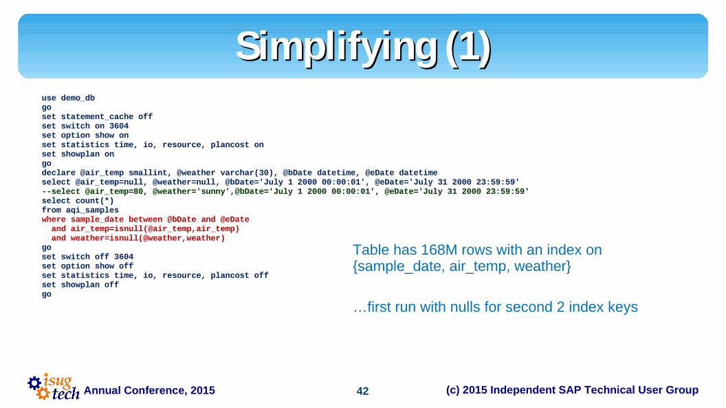
Simplifying (1)Simplifying (1)use demo_dbgoset statement_cache offset switch on 3604set option show onset statistics time, io, resource, plancost onset showplan ongodeclare @air_temp smallint, @weather varchar(30), @bDate datetime, @eDate datetimeselect @air_temp=null, @weather=null, @bDate='July 1 2000 00:00:01', @eDate='July 31 2000 23:59:59'--select @air_temp=80, @weather='sunny',@bDate='July 1 2000 00:00:01', @eDate='July 31 2000 23:59:59'select count(*)from aqi_sampleswhere sample_date between @bDate and @eDate and air_temp=isnull(@air_temp,air_temp) and weather=isnull(@weather,weather)goset switch off 3604set option show offset statistics time, io, resource, plancost offset showplan offgo
Table has 168M rows with an index on {sample_date, air_temp, weather}
…first run with nulls for second 2 index keys

43Annual Conference, 2015 (c) 2015 Independent SAP Technical User Group
Simplifying (2)Simplifying (2)The Lop tree:( project
( scalar( scan aqi_samples)
))
OptBlock1 The Lop tree:( scan aqi_samples)
Generic Tables: ( Gtt1( aqi_samples ) Gti2( aqi_samples_PK ) Gti3( aqi_weather_date_idx ) ) Generic Columns: …Predicates: ( { aqi_samples.sample_date} >= "Jan 1 1900 12:00AM" tc:{3} { aqi_samples.sample_date} <= "Jan 1 1900 12:00AM" tc:{3} ) Transitive Closures: …
OptBlock0 The Lop tree:( pseudoscan)
Generic Tables: ( Gta0 ) Generic Columns: …Predicates: ( ) Transitive Closures: …
The between clause is only one passed to optimizer…not much of a surprise as with the NULLs, we are expecting no-ops on air_temp and weather.
Note that since we don’t know the value of @vars at compile time, we use default date here

44Annual Conference, 2015 (c) 2015 Independent SAP Technical User Group
Simplifying (3)Simplifying (3)Total estimated I/O cost for statement 3 (at line 4): 17133977.
==================== Lava Operator Tree ==================== Emit (VA = 3) r:1 er:1 cpu: 0 / ScalarAgg Count (VA = 2) r:1 er:1 cpu: 400 / Restrict (0)(0)(0)(11)(0) (VA = 1) r:1.303e+006 er:4.202e+007/IndexScanaqi_weather_date(VA = 0)r:1.303e+006 er:4.202e+007l:1969 el:63590p:251 ep:8005
============================================================Table: aqi_samples scan count 1, logical reads: (regular=1969 apf=0 total=1969), physical reads: (regular=8 apf=243 total=251), apf IOs used=243Total actual I/O cost for this command: 10213.Total writes for this command: 0
Execution Time 4.Adaptive Server cpu time: 417 ms. Adaptive Server elapsed time: 417 ms.
Our total IO estimate is 17M+….Our estimated rows (from IndexScan) are off by 30x….which is bad…

45Annual Conference, 2015 (c) 2015 Independent SAP Technical User Group
Simplifying – Rerun (1)Simplifying – Rerun (1)use demo_dbgoset statement_cache offset switch on 3604set option show onset statistics time, io, resource, plancost onset showplan ongodeclare @air_temp smallint, @weather varchar(30), @bDate datetime, @eDate datetime--select @air_temp=null, @weather=null, @bDate='July 1 2000 00:00:01', @eDate='July 31 2000 23:59:59'select @air_temp=80, @weather='sunny',@bDate='July 1 2000 00:00:01', @eDate='July 31 2000 23:59:59'select count(*)from aqi_sampleswhere sample_date between @bDate and @eDate and air_temp=isnull(@air_temp,air_temp) and weather=isnull(@weather,weather)goset switch off 3604set option show offset statistics time, io, resource, plancost offset showplan offgo
Table has 168M rows with an index on {sample_date, air_temp, weather}
…second run with values for second 2 index keys

46Annual Conference, 2015 (c) 2015 Independent SAP Technical User Group
Simplifying - Rerun (2)Simplifying - Rerun (2)The Lop tree:( project
( scalar( scan aqi_samples)
)
)
OptBlock1 The Lop tree:( scan aqi_samples)
Generic Tables: ( Gtt1( aqi_samples ) Gti2( aqi_samples_PK ) Gti3( aqi_weather_date_idx ) ) Generic Columns: …Predicates: ( { aqi_samples.sample_date} >= "Jan 1 1900 12:00AM" tc:{3} { aqi_samples.sample_date} <= "Jan 1 1900 12:00AM" tc:{3} ) Transitive Closures: …
OptBlock0 The Lop tree:( pseudoscan)
Generic Tables: ( Gta0 ) Generic Columns: …Predicates: ( ) Transitive Closures: …
The between clause is still the only one passed to optimizer… which means this fails as a coding style

47Annual Conference, 2015 (c) 2015 Independent SAP Technical User Group
Simplifying - Rerun (3)Simplifying - Rerun (3)Total estimated I/O cost for statement 3 (at line 4): 17133977.
==================== Lava Operator Tree ==================== Emit (VA = 3) r:1 er:1 cpu: 0 / ScalarAgg Count (VA = 2) r:1 er:1 cpu: 300 / Restrict (0)(0)(0)(11)(0) (VA = 1) r:0 er:4.202e+007/IndexScanaqi_weather_date(VA = 0)r:1.303e+006 er:4.202e+007l:1969 el:63590p:0 ep:8005
============================================================Table: aqi_samples scan count 1, logical reads: (regular=1969 apf=0 total=1969), physical reads: (regular=0 apf=0 total=0), apf IOs used=0Total actual I/O cost for this command: 3938.Total writes for this command: 0
Execution Time 3.Adaptive Server cpu time: 309 ms. Adaptive Server elapsed time: 309 ms.
We get the same estimates for total IO (17M) and in the bottom node, but the Restrict filters out non-qualifying rows – so we get 0….and finish 100ms faster…the faster execution might make developer think it worked. However, we do the same amount of work (1969 LIOs) so the faster exec is just likely the reduction in ScalarAgg (which it is) due to fewer rows to count.

48Annual Conference, 2015 (c) 2015 Independent SAP Technical User Group
Simplifying – Correct (1)Simplifying – Correct (1)use demo_dbgoset statement_cache offset switch on 3604set option show onset statistics time, io, resource, plancost onset showplan ongodeclare @air_temp smallint, @weather varchar(30), @bDate datetime, @eDate datetime--select @air_temp=null, @weather=null, @bDate='July 1 2000 00:00:01', @eDate='July 31 2000 23:59:59'select @air_temp=80, @weather='sunny',@bDate='July 1 2000 00:00:01', @eDate='July 31 2000 23:59:59'select count(*)from aqi_sampleswhere sample_date between @bDate and @eDate and air_temp=@air_temp and weather=@weathergoset switch off 3604set option show offset statistics time, io, resource, plancost offset showplan offgo
Table has 168M rows with an index on {sample_date, air_temp, weather}
…third run with the way it should be…

49Annual Conference, 2015 (c) 2015 Independent SAP Technical User Group
Simplifying - Correct (2)Simplifying - Correct (2)The Lop tree:( project
( scalar( scan aqi_samples)
)
)
OptBlock1 The Lop tree:( scan aqi_samples)
Generic Tables: ( Gtt1( aqi_samples ) Gti2( aqi_samples_PK ) Gti3( aqi_weather_date_idx ) ) Generic Columns: …Predicates: ( { aqi_samples.sample_date} >= "Jan 1 1900 12:00AM" tc:{3} { aqi_samples.sample_date} <= "Jan 1 1900 12:00AM" tc:{3}
{ aqi_samples.air_temp} = 0 tc:{2} { aqi_samples.weather} = ' tc:{1} ) Transitive Closures: …
OptBlock0 The Lop tree:( pseudoscan)
Generic Tables: ( Gta0 ) Generic Columns: …Predicates: ( ) Transitive Closures: …
We now have all 3 predicates…since we still have @vars with unknown values, we substitute a 0 for int/smallint and ‘ (empty string) for varchar/char

50Annual Conference, 2015 (c) 2015 Independent SAP Technical User Group
Simplifying - Correct (3)Simplifying - Correct (3)Total estimated I/O cost for statement 3 (at line 4): 227844.
==================== Lava Operator Tree ==================== Emit (VA = 2) r:1 er:1 cpu: 0 / ScalarAgg Count (VA = 1) r:1 er:1 cpu: 0/IndexScanaqi_weather_date(VA = 0)r:0 er:450006l:306 el:1307p:0 ep:165
============================================================Table: aqi_samples scan count 1, logical reads: (regular=306 apf=0 total=306), physical reads: (regular=0 apf=0 total=0), apf IOs used=0Total actual I/O cost for this command: 612.Total writes for this command: 0
Execution Time 0.Adaptive Server cpu time: 1 ms. Adaptive Server elapsed time: 1 ms.
Total estimated IO is 228K (vs. 17M) and estimated rowcount is TONS less…still off, but likely due to data skew and not knowing values of @vars…. And we only do 300 LIO vs. 1969….and we finish 300x faster

51Annual Conference, 2015 (c) 2015 Independent SAP Technical User Group
Index Keys: The QueryIndex Keys: The QuerySELECT SUM( T_00 ."MBGBTR" ) FROM "COEP" T_00
INNER JOIN "COBK" T_01 ON T_01 ."KOKRS" = ? AND T_01 ."BELNR" = T_00 ."BELNR"
WHERE T_00 ."MANDT" = ? AND T_00 ."LEDNR" = ? AND T_00 ."OBJNR" = ? AND ( T_00 ."KSTAR" BETWEEN ? AND ? OR T_00 ."KSTAR" IN ( ? , ? , ? , ? ) ) AND T_01 ."AWTYP" = ? /* R3:ZVDESR121:558 T:COEP M:400 */
index_name index_keys index_description,COEP~0 MANDT, KOKRS, BELNR, BUZEI nonclustered, uniqueCOEP~1 MANDT, LEDNR, OBJNR, GJAHR, WRTTP, VERSN, KSTAR, HRKFT, PERIO,
VRGNG, PAROB, USPOB, VBUND, PARGB, BEKNZ, TWAER nonclusteredCOEP~Z02 MANDT, KOKRS, BUKRS, OBJNR nonclusteredCOEP_BDLS0 MANDT, LOGSYSO nonclusteredCOEP~4 MANDT, TIMESTMP, OBJNR nonclusteredCOEP~Z03 MANDT, LEDNR, OBJNR, KSTAR nonclusteredCOEP~Z05 MANDT, OBJNR, KSTAR, GJAHR, PERIO, PAROB1, WRTTP nonclusteredCOEP~Zt1 MANDT, LEDNR, OBJNR, KSTAR nonclustered

52Annual Conference, 2015 (c) 2015 Independent SAP Technical User Group
Index Keys – Bad Index AccessIndex Keys – Bad Index Access |ROOT:EMIT Operator (VA = 5) | | |SCALAR AGGREGATE Operator (VA = 4) | | Evaluate Ungrouped SUM OR AVERAGE AGGREGATE. | | | | |NESTED LOOP JOIN Operator (VA = 3) (Join Type: Inner Join) | | | | | | |RESTRICT Operator (VA = 1)(0)(0)(0)(4)(0) | | | | | | | | |SCAN Operator (VA = 0) | | | | | FROM TABLE | | | | | COEP | | | | | T_00 | | | | | Index : COEP~4 | | | | | Forward Scan. | | | | | Positioning by key. | | | | | Keys are: | | | | | MANDT ASC | | | | | Using I/O Size 128 Kbytes for index leaf pages. | | | | | With LRU Buffer Replacement Strategy for index leaf pages. | | | | | Using I/O Size 128 Kbytes for data pages. | | | | | With LRU Buffer Replacement Strategy for data pages. | | | | | | |SCAN Operator (VA = 2) | | | | FROM TABLE | | | | COBK | | | | T_01 | | | | Index : COBK~Zt1 | | | | Forward Scan. | | | | Positioning at index start. | | | | Index contains all needed columns. Base table will not be read. | | | | Using I/O Size 16 Kbytes for index leaf pages. | | | | With LRU Buffer Replacement Strategy for index leaf pages.

(c) 2015 Independent SAP Technical User GroupAnnual Conference, 2015
OPTIMIZATION COSTING OPTIMIZATION COSTING (PART 1)(PART 1)
Histograms, Column Densities, IN(), Out of Range Histograms…

54Annual Conference, 2015 (c) 2015 Independent SAP Technical User Group
HistogramsHistogramsThe key to cost-based optimization
q Really is a distribution of data skew
ü If data was evenly distributed, we wouldn’t need histograms at all
q Mostly used for range scansq Can be used for equisargs if
data highly skewed..as most is
The basicsq Frequency cells q Range cells
Statistics for column: "type"Last update of column statistics: Feb 15 2015 9:18:32:850PM
Range cell density: 0.0053191489361702 Total density: 0.4216274332277049 Range selectivity: default used (0.33) In between selectivity: default used (0.25) Unique range values: 0.0053191489361702 Unique total values: 0.2000000000000000 Average column width: default used (2.00) Rows scanned: 188.0000000000000000 Statistics version: 4
Histogram for column: "type"Column datatype: char(2)Requested step count: 20Actual step count: 9Sampling Percent: 0Tuning Factor: 20Out of range Histogram Adjustment is DEFAULT. Low Domain Hashing.
Step Weight Value
1 0.00000000 <= "EJ" 2 0.00531915 < "P " 3 0.10638298 = "P " 4 0.00000000 < "S " 5 0.30319148 = "S " 6 0.00000000 < "U " 7 0.56382978 = "U " 8 0.00000000 < "V " 9 0.02127660 = "V "
Range Cells
Frequency Cells

55Annual Conference, 2015 (c) 2015 Independent SAP Technical User Group
How Many Steps Do We NeedHow Many Steps Do We NeedFewer = better for resource usage and time to find steps
More = better for optimization accuracyq Ideally, you want most range scans to be in a single cell
ü Multiple cells means aggregating stats…may be accurate, but takes longer
ü For example, for datetime, columns see if cells cover the common query range (week, month, year, ….)
Hard to near impossible to control to semantic boundaries
q Increase stats may be better for estimates with high skew

56Annual Conference, 2015 (c) 2015 Independent SAP Technical User Group
Example Date HistogramExample Date HistogramHistogram for column: "sample_date"Column datatype: datetimeRequested step count: 100Actual step count: 103Sampling Percent: 0Tuning Factor: 20Out of range Histogram Adjustment is DEFAULT. Sticky step count. Sticky hashing.
Step Weight Value
1 0.00000000 <= "Jan 1 1993 11:59:59:996AM" 2 0.01017933 <= "Feb 13 1993 12:00:00:000PM" 3 0.00763450 <= "Mar 18 1993 12:00:00:000PM" 4 0.01018039 <= "May 1 1993 12:00:00:000PM" 5 0.00766925 <= "Jun 3 1993 12:00:00:000PM" 6 0.00777507 <= "Jul 6 1993 12:00:00:000PM" 7 0.00825124 <= "Aug 8 1993 12:00:00:000PM" 8 0.00816318 <= "Sep 10 1993 12:00:00:000PM" 9 0.00796063 <= "Oct 13 1993 12:00:00:000PM" 10 0.00795876 <= "Nov 15 1993 12:00:00:000PM" 11 0.00795651 <= "Dec 18 1993 12:00:00:000PM" 12 0.00788510 <= "Jan 19 1994 12:00:00:000PM" 13 0.01000150 <= "Feb 28 1994 12:00:00:000PM" 14 0.01000150 <= "Apr 9 1994 12:00:00:000PM“…
~1.5 month spread…. Problem is that on some months it is mid-month, so a range scan for that month would need 3 cells. If concerned, likely need to double or triple stats

57Annual Conference, 2015 (c) 2015 Independent SAP Technical User Group
Histograms & StepsHistograms & StepsDefault no HTF Defaults 40 steps 100 steps 500 steps
Default number of steps 20 20 20 20 20
Histogram tuning factor 1 20 20 20 20
Requested steps 20 20 40 100 500
Actual steps 20 195 509 1550 7580
(Index statistics for combined city,state)
Range cell density 0.00328457 0.00121356 0.00022722 0.00010744 0.00003560
Total density 0.00328457 0.00328457 0.00328457 0.00328457 0.00328457
Unique range values 0.00011547 0.00008212 0.00006416 0.00004897 0.00002615
Unique total values 0.00011547 0.00011547 0.00011547 0.00011547 0.00011547
Impact on estimates for Washington DC & San Francisco CA
DC Cell <= Washington <= Washington = Washington = Washington = Washington
DC Selectivity 0.05184000 0.02155000 0.02063000 0.02063000 0.02063000
DC Row Estimates 5184 2155 2063 2063 2063
SF Cell <= Somerset <= San Jacint = San Franci = San Franci = San Franci
SF Selectivity 0.04875000 0.00678000 0.00634000 0.00634000 0.00634000
SF Row Estimates 4875 678 634 634 634
Statistics from an index on {city,state} for a 100,000 row table with ~6,200 distinct city names

58Annual Conference, 2015 (c) 2015 Independent SAP Technical User Group
Column DensitiesColumn DensitiesSingle column densities
q Range cell density/unique range values
ü Tells maximum uniqueness…
ü Min(weight)!=0 from range cells
q Total densityü Relative skewness of the
dataü Total density approaching
1.0 is extremely skewed
ü Sum(weights^2)q Unique total values
ü The number distinct values in column
ü 1.0/select count(distinct column)
Multiple column densitiesq Automatically created on index
leading keysq May be manually createdq More on this later
Statistics for column: "type"Last update of column statistics: Feb 15 2015 9:18:32:850PM
Range cell density: 0.0053191489361702 Total density: 0.4216274332277049 Range selectivity: default used (0.33) In between selectivity: default used (0.25) Unique range values: 0.0053191489361702 Unique total values: 0.2000000000000000 Average column width: default used (2.00) Rows scanned: 188.0000000000000000 Statistics version: 4
Statistics for column group: "sample_date", "air_temp", "weather"Last update of column statistics: May 27 2014 11:45:45:016AM
Range cell density: 0.0000051075008894 Total density: 0.0000051075008894 Range selectivity: default used (0.33) In between selectivity: default used (0.25) Unique range values: 0.0000016297687032 Unique total values: 0.0000016297687032 Average column width: 8.5268955638740458 Rows scanned: 168066824.0000000000000000 Statistics version: 4

59Annual Conference, 2015 (c) 2015 Independent SAP Technical User Group
Using Column DensitiesUsing Column DensitiesI f the column value is known and…
q …value falls in a range cell ….Estimate will be range cell valueü Whether range or frequency cell
I f the column value is not knownq Optimized with a literal placeholder (0, ‘’, Jan 1 1900,
etc.)q Selectivity is total density

60Annual Conference, 2015 (c) 2015 Independent SAP Technical User Group
Column Selectivity vs. Density (1)Column Selectivity vs. Density (1)Statistics for column: "id"Last update of column statistics: Feb 16 2015 4:47:23:956PM
Range cell density: 0.0092592412744228 Total density: 0.0113194187537711 Unique range values: 0.0041383133267069 Unique total values: 0.0055248618784530
Step Weight Value
1 0.00000000 < 1 2 0.01093356 = 1 3 0.01387721 <= 2 4 0.01261564 <= 3 5 0.00714886 <= 4 6 0.00294365 <= 5 7 0.00462574 <= 6 8 0.00210261 <= 8 9 0.00336417 <= 9 10 0.00336417 <= 11 11 0.00378469 <= 12 12 0.00925147 <= 13 13 0.00210261 <= 15 14 0.01808242 <= 16 15 0.00252313 <= 17 16 0.00252313 <= 18 17 0.00168209 <= 19 18 0.00000000 < 21 19 0.00630782 = 21 20 0.00252313 <= 22 21 0.01429773 <= 23 22 0.03868797 <= 24 23 0.00378469 <= 25
1> declare @id int2> select @id=83> select * from syscolumns where id=@id
Estimating selectivity of index 'syscolumns.csyscolumns', indid 2 id = 0 Estimated selectivity for id, selectivity = 0.01131942, scan selectivity 0.01131942, filter selectivity 0.01131942 26.91758 rows, 1 pages
range cell unknown
1> select * from syscolumns where id=8
Estimating selectivity of index 'syscolumns.csyscolumns', indid 2 id = 8 Estimated selectivity for id, selectivity = 0.002102607, scan selectivity 0.002102607, filter selectivity 0.002102607 5 rows, 1 pages
Weight < range cell density q selectivity = weight

61Annual Conference, 2015 (c) 2015 Independent SAP Technical User Group
Column Selectivity vs. Density (2)Column Selectivity vs. Density (2)Statistics for column: "id"Last update of column statistics: Feb 16 2015 4:47:23:956PM
Range cell density: 0.0092592412744228 Total density: 0.0113194187537711 Unique range values: 0.0041383133267069 Unique total values: 0.0055248618784530
Step Weight Value
1 0.00000000 < 1 2 0.01093356 = 1 3 0.01387721 <= 2 4 0.01261564 <= 3 5 0.00714886 <= 4 6 0.00294365 <= 5 7 0.00462574 <= 6 8 0.00210261 <= 8 9 0.00336417 <= 9 10 0.00336417 <= 11 11 0.00378469 <= 12 12 0.00925147 <= 13 13 0.00210261 <= 15 14 0.01808242 <= 16 15 0.00252313 <= 17 16 0.00252313 <= 18 17 0.00168209 <= 19 18 0.00000000 < 21 19 0.00630782 = 21 20 0.00252313 <= 22 21 0.01429773 <= 23 22 0.03868797 <= 24 23 0.00378469 <= 25
1> select * from syscolumns where id=21
Estimating selectivity of index 'syscolumns.csyscolumns', indid 2 id = 21 Estimated selectivity for id, selectivity = 0.006307822, scan selectivity 0.006307822, filter selectivity 0.006307822 15 rows, 1 pages
Frequency cell � selectivity = weight
1> select * from syscolumns where id=24
Estimating selectivity of index 'syscolumns.csyscolumns', indid 2 id = 24 Estimated selectivity for id, selectivity = 0.03868797, scan selectivity 0.03868797, filter selectivity 0.03868797 92 rows, 1 pages
Weight > range cell density q selectivity = weight

62Annual Conference, 2015 (c) 2015 Independent SAP Technical User Group
Column Selectivity vs. Density (3)Column Selectivity vs. Density (3)Statistics for column: "id"Last update of column statistics: Feb 16 2015 4:47:23:956PM
Range cell density: 0.0092592412744228 Total density: 0.0113194187537711 Unique range values: 0.0041383133267069 Unique total values: 0.0055248618784530
Step Weight Value
1 0.00000000 < 1 2 0.01093356 = 1 3 0.01387721 <= 2 4 0.01261564 <= 3 5 0.00714886 <= 4 6 0.00294365 <= 5 7 0.00462574 <= 6 8 0.00210261 <= 8 9 0.00336417 <= 9 10 0.00336417 <= 11 11 0.00378469 <= 12 12 0.00925147 <= 13 13 0.00210261 <= 15 14 0.01808242 <= 16 15 0.00252313 <= 17 16 0.00252313 <= 18 17 0.00168209 <= 19 18 0.00000000 < 21 19 0.00630782 = 21 20 0.00252313 <= 22 21 0.01429773 <= 23 22 0.03868797 <= 24 23 0.00378469 <= 25
1> select * from syscolumns where id between 5 and 10
Estimating selectivity of index 'syscolumns.csyscolumns', indid 2 id >= 5 id <= 10 Estimated selectivity for id, selectivity = 0.01471826, scan selectivity 0.01471826, filter selectivity 0.01471826 35.00002 rows, 1 pages
Range query
Note that the sum of steps 6• 10 is 0.01640034. However, since we are only using a portion of step 10 and the distribute is 2 values per step, we use the formula:
Sum(step6..step9) + step10/2.0 = 0.01471826

63Annual Conference, 2015 (c) 2015 Independent SAP Technical User Group
Debugging SelectivityDebugging SelectivityYou’ve probably noticed….
q You need to have ‘set option show’ and optdiag outputFind the index you thought it should have used
q Look at the selectivity for each predicateq Check out the optdiag to see if it was a really skewed
valueBut sometimes you just have to look at the query
q …your expectation may be due to knowledge you inferü But optimizer doesn’t knowü ….such as the relationship between two columns
q …and sometimes the indexing doesn’t support the query
64Annual Conference, 2015 (c) 2015 Independent SAP Technical User Group
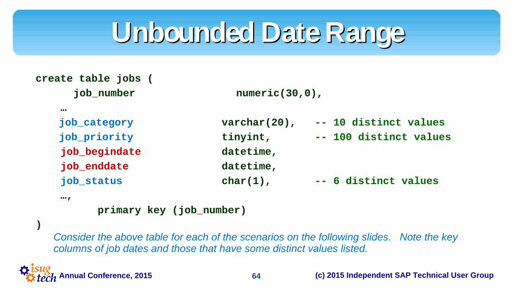
Unbounded Date RangeUnbounded Date Rangecreate table jobs (
job_number numeric(30,0), …
job_category varchar(20), -- 10 distinct valuesjob_priority tinyint, -- 100 distinct values
job_begindate datetime, job_enddate datetime,
job_status char(1), -- 6 distinct values …, primary key (job_number)
)Consider the above table for each of the scenarios on the following slides. Note the key columns of job dates and those that have some distinct values listed.

65Annual Conference, 2015 (c) 2015 Independent SAP Technical User Group
Scenario #1Scenario #1Consider the index:
create index job_begin_idx on jobs (job_begindate)
…and the typical query Select * from jobs Where job_begindate >= $begin_date and job_enddate <= $end_date
Why is LIO sometimes high and sometimes low?

66Annual Conference, 2015 (c) 2015 Independent SAP Technical User Group
Scenario #1: The ProblemsScenario #1: The ProblemsBecause the index only has begin date
q On very recent dates, it can go near the end of the index and scan to the end…
q But on dates in the past – even a few months agoü It positions to the $begin_dateü Scans to end of indexü For each leaf node, it does a LIO to data page
to compare $end_dateü Some quick math….assume 50 rows per page
per index leaf node 100 leaf pages = 5000 data page LIO’s ≈ 1
sec CPU (@5LIO/ms) 1000 leaf pages = 50000 data page LIO’s
≈ 10 sec CPU 10000 leaf pages = 500000 data page
LIO’s ≈ 100 sec CPU 100000 leaf pages = 5000000 data page
LIO’s ≈ 1000 sec CPU (16m40s)Soooo….
q For dates not very recent, we get an index leaf scan to end of index
q Plus a datapage lookup for every leaf row
2010
2011
2012
2013
2014
> 01Mar2011
> 01Nov2012
> 01Jan2014

67Annual Conference, 2015 (c) 2015 Independent SAP Technical User Group
Scenario #1: The SolutionsScenario #1: The SolutionsSolution #1: Add job_enddate to index
create index job_date_idx on jobs (job_begindate, job_enddate)
Solution #2: Add implied boundary to date query Select * from jobs Where job_begindate between $begin_date and $end_date and job_enddate between $begin_date and $end_date
Why both???q Wouldn’t fixing the index be enough – why bother the
coders and try to teach them better coding style???

68Annual Conference, 2015 (c) 2015 Independent SAP Technical User Group
Scenario #2Scenario #2Consider the index:
create index job_begin_idx on jobs (job_category, job_begindate)
…and the typical query Select * from jobs Where job_begindate >= $begin_date and job_enddate <= $end_date
Why does it sometimes use the index and other times not?

69Annual Conference, 2015 (c) 2015 Independent SAP Technical User Group
Scenario #2: The ProblemScenario #2: The ProblemThe problem is we are missing a predicate on leading index columns
q A similar situation occurs when we have intermediate index keys for which we have no valid SARGs
To handle this, ASE does a bit of a trickq It looks at cardinality of unknown keys
ü If low it considers an ORScan for each valueü If high, it considers an index leaf scan
q Then it considers the selectivity of the known predicatesSooo…as a result
q If we pick a date that is fairly recent (index is more selective), then we will likely do an ORScan and then a index leaf scan from the begin date until the next job_category
q If we pick a date that isn’t very selective, then the ORScan becomes too expensive due to leaf scan per Orscan and we compare the multiple index leaf scan vs. single table scan

70Annual Conference, 2015 (c) 2015 Independent SAP Technical User Group
Scenario #2: The SolutionScenario #2: The SolutionSolution: Add implied boundary to date query
Select * from jobs Where job_begindate between $begin_date and $end_date and job_enddate between $begin_date and $end_date
…and this is why we fix both the index and the queryq In the above case, considering the index in scenario #2,
as long as the range is fairly selective, we likely will do the ORScan
71Annual Conference, 2015 (c) 2015 Independent SAP Technical User Group
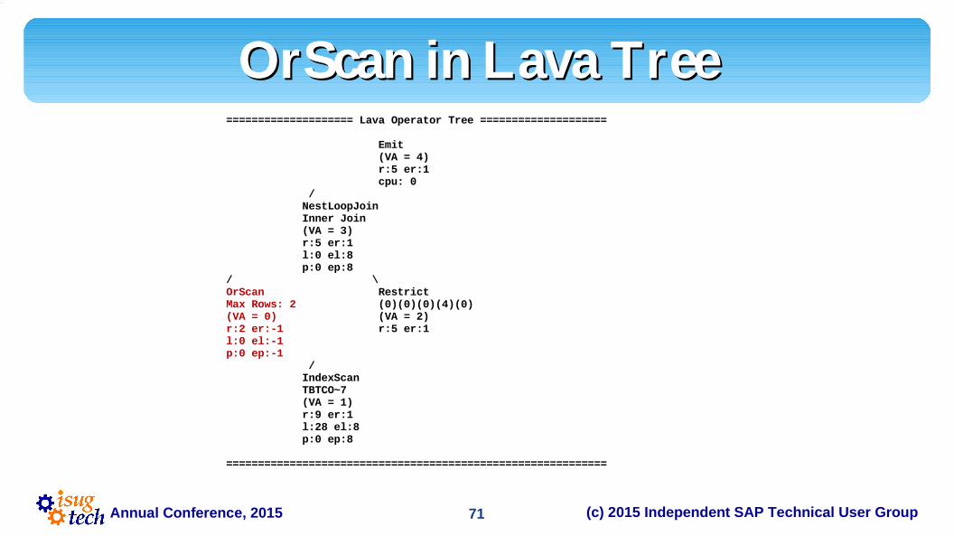
OrScan in Lava TreeOrScan in Lava Tree==================== Lava Operator Tree ==================== Emit (VA = 4) r:5 er:1 cpu: 0 / NestLoopJoin Inner Join (VA = 3) r:5 er:1 l:0 el:8 p:0 ep:8/ \OrScan RestrictMax Rows: 2 (0)(0)(0)(4)(0)(VA = 0) (VA = 2)r:2 er:-1 r:5 er:1l:0 el:-1p:0 ep:-1 / IndexScan TBTCO~7 (VA = 1) r:9 er:1 l:28 el:8 p:0 ep:8
============================================================

72Annual Conference, 2015 (c) 2015 Independent SAP Technical User Group
OrScan in Show PlanOrScan in Show Plan |ROOT:EMIT Operator (VA = 6) | | |NESTED LOOP JOIN Operator (VA = 5) (Join Type: Inner Join) | | | | |NESTED LOOP JOIN Operator (VA = 3) (Join Type: Inner Join) | | | | | | |SCAN Operator (VA = 0) | | | | FROM OR List | | | | OR List has up to 12 rows of OR/IN values. | | | | | | |RESTRICT Operator (VA = 2)(0)(0)(0)(13)(0) | | | | | | | | |SCAN Operator (VA = 1) | | | | | FROM TABLE | | | | | SAPSR3.MSEG | | | | | T_01 | | | | | Index : MSEG~1 | | | | | Forward Scan. | | | | | Positioning by key. | | | | | Keys are: | | | | | MANDT ASC | | | | | MATNR ASC | | | | | Using I/O Size 128 Kbytes for index leaf pages. | | | | | With LRU Buffer Replacement Strategy for index leaf pages. | | | | | Using I/O Size 128 Kbytes for data pages. | | | | | With LRU Buffer Replacement Strategy for data pages. | |

73Annual Conference, 2015 (c) 2015 Independent SAP Technical User Group
Scenario #3Scenario #3Consider the following index
create index job_begin_idx on jobs (job_category, job_status, job_begindate, job_enddate)
…and the typical query Select * from jobs Where job_category = ‘night batch’ and job_status in (‘U’, ‘A’, ‘E’) and job_begindate >= $begin_date and job_enddate <= $end_date
Why might we only position by job_category, job_status?

74Annual Conference, 2015 (c) 2015 Independent SAP Technical User Group
Scenario #3: The ProblemScenario #3: The ProblemThe problem is we don’t have multi-density stats
q And creating them might be a bit of a nightmareAs a result, ASE does the following
q It weighs each selectivity individually:ü ‘nightly batch’ + ‘U’ + $begin_dateü ‘nightly batch’ + ‘A’ + $begin_dateü ‘nightly batch’ + ‘E’ + $begin_date
q Then aggregates Here’s the problem….assume we only have 20 steps
q Let’s pick a begin date 3 or more steps from the endü …and assume end_date is in the same stepü …but remember, we have an unbounded range on both ….so
…effectively it will think it will be 3 steps for each $begin_date….not 1 …and it will thing $end_date is atrocious as is 17 steps worth (from beginning)
q If we aggregate, then we will have 3x….so 9 steps….40% of table is 8 steps….we might table scan or look for different index

75Annual Conference, 2015 (c) 2015 Independent SAP Technical User Group
Scenario #3: The SolutionScenario #3: The SolutionUpdate column stats for distinctive columns
q Use 100 steps or similar large valueü update statistics job_status (job_begindate) using 100
values
q Result is that each step has a much lower selectivity value
Add the bounded range into the queryq This means we aggregate only across the exact range of
dates we want…which reduces the impact of the IN() clause
q

76Annual Conference, 2015 (c) 2015 Independent SAP Technical User Group
ASE’s OR StrategyASE’s OR StrategyI f the query contains an OR clause on different columns
q ASE will (and can) use two different indexesü On index for predicates on one side of ORü …and a different index for predicates on other side of
ORü This would be similar to splitting the query in two with
unionq However, if one side of OR drives a tablescan – ASE will
tablescan ü Remember, we saw this with the id=8 OR 1=2
exampleCommon issues
q One side of OR not indexed well….drives tablescanq Developer attempted to use 1 index to cover both
columns in ORü In order for OR strategy to work, you always need 2 indexes!!!!

77Annual Conference, 2015 (c) 2015 Independent SAP Technical User Group
An Example of Indexing vs. ORAn Example of Indexing vs. ORConsider the following query:
SELECT "VBELV" ,"POSNV" ,"VBELN" ,"POSNN" ,"VBTYP_N" ,"RFMNG" ,"MEINS" ,"VBTYP_V" ,"ERDAT" ,"ERZET" ,"AEDAT" ,"STUFE" ,"VRKME" FROM "VBFA" WHERE "MANDT" = ? AND ( "ERDAT" = ? OR "AEDAT" = ? ) /* R3:SAPLZFEDWS1:767 T:VBFA M:430 */
Now, consider the indexes: index_name index_keys -------------------------------------
-------------------------------------------- VBFA~0 MANDT, VBELV, POSNV, VBELN, POSNN, VBTYP_N VBFA~Z01 MANDT, VBELN VBFA~Z02 ERDAT, BWART VBFA~Z04 MANDT, ERDAT, AEDAT VBFA~Z99 MANDT, LOGSYS
Issue is that the query seems to drive a tablescan….q …it seems obvious that VBFA~Z04 should be used…..q ….or is it???

78Annual Conference, 2015 (c) 2015 Independent SAP Technical User Group
Let’s look a little closerLet’s look a little closerLooking at systabstats
ColumnName ColumnID Row_Count RequestedSteps ActualSteps ApproxDistincts DistinctsPerStep
-------------- -------- -------------------- -------------- ----------- --------------- -----------------
AEDAT 22 1255008198 50 50 1625 33.0
BWART 17 1255008198 50 29 64 2.0
ERDAT 14 1255008198 50 245 4674 19.0
LOGSYS 38 1255008198 50 2 1 1.0
MANDT 1 1255008198 50 2 1 1.0
POSNN 5 1255008198 50 573 93300 163.0
POSNV 3 1255008198 50 231 12649 55.0
VBELN 4 1255008198 50 38 85330918 2245550.0
VBELV 2 1255008198 50 38 31223216 821664.0
VBTYP_N 6 1255008198 50 31 25 1.0
Hmmmm….not very good query criteriaq MANDT is useless as alwaysq AEDAT and ERDAT are not very distinct….1625 and 4674 values
respectivelyü Which means each distinct value will return ~250K to ~1M
rows respectively Just a SWAG based on 1 billion rows divided by 1000 and 4000 respectively Of course, this assumes EVEN distribution of values…. …which we all know business…..everything happens in the last month of the
quarter, etc….so expecting some heavy skewü But it means we *could* be retrieving 1 million rows
legitimately…..REALLY???

79Annual Conference, 2015 (c) 2015 Independent SAP Technical User Group
AEDAT Stats….from optdiagAEDAT Stats….from optdiagStatistics for column: AEDATLast update of column statistics: Jan 10 2014 7:21:35:026PMRange cell density: 0.0000017268359901Total density: 0.9986527756879466…Unique range values: 0.0000004149259654Unique total values: 0.0006153846153846…
Histogram for column: AEDATColumn datatype: varchar(24)…
Statistics step count stickyStatistics hashing stickyStatistics hashing low domain used
Step Weight Value (only 255 bytes used)
1 0.00000000 < '00000000' 2 0.99932617 = '00000000' 3 0.00001720 <= '20080724' 4 0.00001430 <= '20080826' 5 0.00001409 <= '20081030' 6 0.00001545 <= '20081113' 7 0.00001415 <= '20081216' 8 0.00001419 <= '20090310' 9 0.00001468 <= '20090331' 10 0.00002772 <= '20090615' …
OUCH!!!!!

80Annual Conference, 2015 (c) 2015 Independent SAP Technical User Group
ERDAT Stats….from optdiagERDAT Stats….from optdiagStatistics for column: ERDATLast update of column statistics: Jan 10 2014 7:21:35:026PMRange cell density: 0.0005738551548958Total density: 0.0006834762135235…Unique range values: 0.0001879716956084Unique total values: 0.0002139495079161…
Requested step count: 50Actual step count: 245…
Statistics step count stickyStatistics hashing stickyStatistics hashing low domain used
Step Weight Value (only 255 bytes used)
1 0.00000000 < '00000000' 2 0.00004201 = '00000000' 3 0.01879592 <= '20030624' 4 0.01879998 <= '20040316' 5 0.01888011 <= '20041015' 6 0.01887963 <= '20050502' 7 0.01878721 <= '20051031' 8 0.01888958 <= '20060420' 9 0.01879898 <= '20061014' 10 0.01882141 <= '20070417'
BETTER!!!!

81Annual Conference, 2015 (c) 2015 Independent SAP Technical User Group
To understand, let’s simplify thingsTo understand, let’s simplify thingsAssume we have a table of customer transactions…
q with 1 billion rowsq PKEY is transaction_id (not that it matters…..)q Has an index (IDX~1) on {purchase_date, ship_date}
ü Both purchase_date and ship_date are not very distinct ü think about it …only 365 in a year….~3600 in 10 years…
not very distinctive out of 1 billion row tableNow consider the query:
Select * from cust_transactions where purchase_date=‘Jan 1 2014’ OR ship_date=‘Jan 1 2014’
See the problem?.... Think about it….

82Annual Conference, 2015 (c) 2015 Independent SAP Technical User Group
The ProblemThe ProblemThe problem query:
Select * from cust_transactions where purchase_date=‘Jan 1 2014’ OR ship_date=‘Jan 1 2014’
The problems….q We can use the index IDX~1 for the purchase_date case …..depending
of course on selectivity of the data providedq …but the OR clause means it that we also need to look for the ship date
ü individually and not in combination with purchase date – remember a composite index works on COMBINING cols
q ….using IDX~1 for that is sort of useless as we can’t use the leading purchase_date column as the OR clause is disjunctive…..the query really could be expressed as:
select * from cust_transactions where purchase_date=‘Jan 1 2014’ union select * from cust_transactions where ship_date=‘Jan 1 2014’

83Annual Conference, 2015 (c) 2015 Independent SAP Technical User Group
Remember special OR strategy???Remember special OR strategy???When an OR condition exists:
q ASE can use multiple indexes – a different index for each side of the OR
q This ‘special OR strategy’ is also known as ‘index union’When looking at the query & index
q ASE says index is probably okay for purchase_date….q ….but says it will need to tablescan for ship_dateq Why the tablescan
ü Remember, this is a DOL table and the index keys are sorted by purchase_date, then ship_date
ü ….so we would have to scan ALL the leaf pages to find that ship_date
ü ….only to find out that 1/4000th of the table qualifiesü ….and they are scattered around due to purchase date,
so….LIO exceeds cost of tablescan so we do tablescanü ….especially if we have an OR value of ‘00000000’….which is
99% of the table.

84Annual Conference, 2015 (c) 2015 Independent SAP Technical User Group
What about IN()???What about IN()???I f you were watching closely….you already know the answerI f you think about it….
q …an IN() is like an OR list…q ….in fact ASE flattens into one
So, all we do is:q Cost each one individuallyq Aggregate them into a final cost

85Annual Conference, 2015 (c) 2015 Independent SAP Technical User Group
A Simple IN() exampleA Simple IN() example1> select * from sysobjects where id in (2,4,6,8,10,12,14,16)The Lop tree:( project
( scan sysobjects)
)
OptBlock0 The Lop tree:( scan sysobjects)
Generic Tables: ( Gtt0( sysobjects ) Gti1( csysobjects ) ) Generic Columns: … Predicates: ( ( { sysobjects.id } = 16 tc:{25} OR{ sysobjects.id } = 14 tc:{25}
OR { sysobjects.id } = 12 tc:{25} OR{ sysobjects.id } = 10 tc:{25} OR { sysobjects.id } = 8 tc:{25} OR{ sysobjects.id } = 6 tc:{25} OR { sysobjects.id } = 4 tc:{25} OR{ sysobjects.id } = 2 tc:{25} ) tc:{25} )
Transitive Closures: …)
IN() clause is expanded to OR’s….note that all have the same transitive closure id (tc:{25})

86Annual Conference, 2015 (c) 2015 Independent SAP Technical User Group
Individual OR term selectivityIndividual OR term selectivityBEGIN GENERAL OR ANALYSIS OF all types of indices FOR sysobjectsANALYZING OR TERM 1
Estimating selectivity of index 'sysobjects.csysobjects', indid 3 id = 16 Estimated selectivity for id, selectivity = 0.1, scan selectivity 0.02272727, filter selectivity 0.02272727 restricted selectivity 0.1 unique index with all keys, one row scans 1 rows, 1 pages…
ANALYZING OR TERM 2
Estimating selectivity of index 'sysobjects.csysobjects', indid 3 id = 14…
ANALYZING OR TERM 3
Estimating selectivity of index 'sysobjects.csysobjects', indid 3 id = 12…
ANALYZING OR TERM 4
Estimating selectivity of index 'sysobjects.csysobjects', indid 3 id = 10…
==================== Lava Operator Tree ==================== Emit (VA = 3) r:8 er:5 cpu: 0 / NestLoopJoin Inner Join (VA = 2) r:8 er:5 l:0 el:5 p:0 ep:4 / \ OrScan IndexScan Max Rows: 8 csysobjects (VA = 0) (VA = 1) r:8 er:-1 r:8 er:5 l:0 el:-1 l:12 el:5 p:0 ep:-1 p:0 ep:4 ============================================================

87Annual Conference, 2015 (c) 2015 Independent SAP Technical User Group
Aggregating Selectivity for ORAggregating Selectivity for OREND GENERAL OR ANALYSIS FOR all types of indices - INDICES FOUND FOR ALL OR TERMS
Scan on table sysobjects skipped because table scan less than concurrency thresholdEstimating selectivity of index 'sysobjects.csysobjects', indid 3 Estimated selectivity for id, selectivity = 0.8, scan selectivity 0.8, filter selectivity 0.8 restricted selectivity 1 special or terms 8 35.2 rows, 1 pages Data Row Cluster Ratio 0.99999 Index Page Cluster Ratio 1 Data Page Cluster Ratio 1 using no index prefetch (size 4K I/O) in index cache 'default data cache' (cacheid 0) with LRU replacement
using no table prefetch (size 4K I/O) in data cache 'default data cache' (cacheid 0) with LRU replacement Data Page LIO for 'csysobjects' on table 'sysobjects' = 1.600336
Whoa!!! Prediction is 80% of the table…which had 44 rows….thankfully in *this* case, it still was only 1 page

88Annual Conference, 2015 (c) 2015 Independent SAP Technical User Group
Aggregating IN()Aggregating IN()Aggregation is unintelligent
q It doesn’t check how many are from same range cellResult is the aggregated value is often over-inflated
TIP: Make sure you have histogram steps > largest IN() listq For SAP systems, this will be 100

89Annual Conference, 2015 (c) 2015 Independent SAP Technical User Group
Out of range histogramsOut of range histogramsOriginally added to ASE 15.0 for monotonic sequences
q For example, sequential numbers, datetime (e.g. current datetime)
q Often times if stats only updated every week, a large portion of the new data values where higher than the histogram range
ü As a result, the optimizer would estimate 0 values and select an index based on that reduced cost estimate whereas in reality there could be millions of rows
q With out of range histograms, several factors are used to estimate how many data values exist beyond the last histogram cell and cost is adjusted higher
Usually in such cases, out of range histograms is a sign of stale statsq ….but for high insert/append use cases, you may be updating or
re-reading a row that was just inserted – e.g. reporting on today’s sales
q ASE 16.0 sp01 adds Dynamic Out of Range Histograms to deal with this problem
q An alternative is to disable out of range stats….

90Annual Conference, 2015 (c) 2015 Independent SAP Technical User Group
Low Cardinality ExamplesLow Cardinality ExamplesHistogram tuning may be a bad thing for short duration “STATUS” columns
q Most of the values in the histogram will be “C” for completeq Unless there is a “permanent” status higher than “U” for
unprocessed, it is unlikely that update stats will catch a “U” value
ü During migration, the system is likely quiesced with nothing incomplete
ü Post-migration, if stats are run during quiet period, likely no incomplete values exist
q Out of range histogram throws off optimizer….0 would have been better estimate
ü Running update stats on weekends or nights when quiet simply causes same problem…as jobs are likely all complete
q Spotted with ‘set option show on’May also happen with very low cardinality “TYPE” columns
q Or any very low cardinality column, in reality when value in predicate is extremely low occurrence in a very low cardinality column and value is higher than more common value(s)

91Annual Conference, 2015 (c) 2015 Independent SAP Technical User Group
Example HistogramExample HistogramHistogram for column: "ENTRY_TYPE"…Out of range Histogram Adjustment is DEFAULT. Sticky step count. Sticky partial_hashing.
Step Weight Value
1 0.00000000 < "C" 2 1.00000000 = "C"
Histogram for column: "STATUS"…Out of range Histogram Adjustment is DEFAULT. Low Domain Hashing. Sticky step count. Sticky partial_hashing.
Step Weight Value
1 0.00000000 < "C" 2 0.98791176 = "C" 3 0.00084806 < "T" 4 0.01124019 = "T"

92Annual Conference, 2015 (c) 2015 Independent SAP Technical User Group
Example ‘set option show output’Example ‘set option show output’Estimating selectivity of index 'SAPSR3.ESH_EX_CPOINTER.ESH_EX_CPOINTER~ST', indid 3 STATUS = 'U' ENTRY_TYPE = 'P' Estimated selectivity for ENTRY_TYPE, Out of range histogram adjustment, selectivity = 0.3333333, Estimated selectivity for STATUS, Out of range histogram adjustment, selectivity = 0.2, scan selectivity 0.2, filter selectivity 0.2 60412.2 rows, 34.2 pages Data Row Cluster Ratio 0.9924527 Index Page Cluster Ratio 0.218543 Data Page Cluster Ratio 0.02202437 using index prefetch (size 128K I/O) Large IO selected: The number of leaf pages qualified is > MIN_PREFETCH pages in index cache 'default data cache' (cacheid 0) with LRU replacement

93Annual Conference, 2015 (c) 2015 Independent SAP Technical User Group
To prevent out of range histogramsTo prevent out of range histogramsTurn off for update statistics
q Turn off for columns – not a whole table or specific indexq Syntax
update statistics table_name [[partition data_partition_name] [ (column1, column2, …) | (column1), (column2), …] | index_name [partition index_partition_name]] [using step values | [out_of_range [on | off| default]]] [with consumers = consumers][, sampling=N percent] [, no_hashing | partial_hashing | hashing] [, max_resource_granularity = N [percent]] [, histogram_tuning_factor = int ] [, print_progress = int]
q Example Update statistics SAPSR3.ESH_EX_CPOINTER (ENTRY_TYPE) out_of_range off Update statistics SAPSR3.ESH_EX_CPOINTER (STATUS) out_of_range off
Out of range histogram is “sticky”q Just like the number of steps, setting this once causes it to be used as
the default for all future update statistics that does not specify a value.

(c) 2015 Independent SAP Technical User GroupAnnual Conference, 2015
OPTIMIZATION COSTING OPTIMIZATION COSTING (PART 2)(PART 2)
Multi-Column Densities & Joins…

95Annual Conference, 2015 (c) 2015 Independent SAP Technical User Group
Multi-Column DensitiesMulti-Column DensitiesA underused secret weapon
q Useful any time multiple predicates existq Think of it this way:
ü Two sample predicates Col_A = ‘5’ Col_B = ‘GREEN’
ü Assume both have a selectivity of 0.1 Combination could still be 0.1 if all Col_A=5 and Col_B=‘GREEN’ are same rows Combination could be 0.01 (or less) if only a single row had the combination
When does it matterq Joins, distinct, subquery (caching), sort estimations, ….q Anyplace where the estimated number of rows returning
could change the query plan (and tip costs towards an alternative ‘bad’ plan)
q Especially since we don’t have composite column histograms

96Annual Conference, 2015 (c) 2015 Independent SAP Technical User Group
Multi-Column Density (Index)Multi-Column Density (Index)Statistics for index: "aqi_weather_date_idx" (nonclustered)Index column list: "sample_date", "air_temp", "weather" Leaf count: 254345 Data page CR count: 167946797.0000000000000000 Index page CR count: 32018.0000000000000000 Data row CR count: 168066295.0000000000000000 Leaf row size: 6.1150672008890936 Index height: 3
Statistics for column group: "sample_date", "air_temp"Last update of column statistics: May 27 2014 11:45:45:016AM
Range cell density: 0.0000051768562637 Total density: 0.0000051768562637 Range selectivity: default used (0.33) In between selectivity: default used (0.25) Unique range values: 0.0000016563476210 Unique total values: 0.0000016563476210 Average column width: default used (2.00) Rows scanned: 168066824.0000000000000000 Statistics version: 4
Statistics for column group: "sample_date", "air_temp", "weather"Last update of column statistics: May 27 2014 11:45:45:016AM
Range cell density: 0.0000051075008894 Total density: 0.0000051075008894 Range selectivity: default used (0.33) In between selectivity: default used (0.25) Unique range values: 0.0000016297687032 Unique total values: 0.0000016297687032 Average column width: 8.5268955638740458 Rows scanned: 168066824.0000000000000000 Statistics version: 4
This is the cost of a covered query (less any portion of index not needed)
The ‘weather’ column must not be very distinct as it doesn’t alter the table total density or range density by very much
If the IO cost of the index is ~page count and the IO cost for the table is near the leaf count – it is doing an index scan and then following each leaf…. Often not a good strategy unless only a few rows
Any NL join using this index would need to traverse the index tree this many times per outer row
(Note: Index cluster ratios removed due to space)

97Annual Conference, 2015 (c) 2015 Independent SAP Technical User Group
Using a Multi-Column DensityUsing a Multi-Column DensityRemember, we don’t have composite histogramsFirst we consider the selectivity of each of the columns individually
q This gives us an idea of how many rows there could beq For example, col_A has 2 rows & col_B has 5 rows….
ü Total range is between 2 & 10 rowsü Probability is likely closer to 2…but depends on
reality….Then we look at multi-column density
q This is our flavor of reality to temper probabilityq We use the above with a proprietary formula to compute
the selectivityü The more selective each column, the closer to the
multi-column density

98Annual Conference, 2015 (c) 2015 Independent SAP Technical User Group
Example: Multi-Column DensityExample: Multi-Column Density
Statistics for column group: "sample_date", "air_temp", "weather"Last update of column statistics: May 27 2014 11:45:45:016AM
Range cell density: 0.0000051075008894 Total density: 0.0000051075008894 Range selectivity: default used (0.33) In between selectivity: default used (0.25) Unique range values: 0.0000016297687032 Unique total values: 0.0000016297687032 Average column width: 8.5268955638740458 Rows scanned: 168066824.0000000000000000 Statistics version: 4
1> select l.city, l.county, s.sample_date, s.air_temp2> from aqi_locations l, aqi_samples s3> where l.location_id=s.location_id4> and s.sample_date = 'July 1 2000 12:00:00:000PM'5> and l.state='PA'6> and s.weather='Overcast'7> and s.air_temp = 90
Estimating selectivity of index 'aqi_samples.aqi_weather_date_idx', indid 3 sample_date= Jul 1 2000 12:00:00:000PM weather = 'Overcast' air_temp = 90 Estimated selectivity for sample_date, selectivity = 0.0002490077, Estimated selectivity for air_temp, selectivity = 0.01104084, Estimated selectivity for weather, selectivity = 0.002359544, scan selectivity 5.11258e-006, filter selectivity 5.11258e-006 859.2551 rows, 1.300359 pages Data Row Cluster Ratio 3.186365e-006 Index Page Cluster Ratio 0.9989935 Data Page Cluster Ratio 0.0007121012 using no index prefetch (size 4K I/O) in index cache 'default data cache' (cacheid 0) with LRU replacement
using no table prefetch (size 4K I/O) in data cache 'default data cache' (cacheid 0) with LRU replacement Data Page LIO for 'aqi_weather_date_idx' on table 'aqi_samples' = 859.2551
Selectivity based single histogram cell for sample_date
Selectivity based single histogram cell for air_temp
Selectivity based on single histogram cell for weather
Selectivity estimate based on numbers of values for the above combined with multi-cell density. Since only a few values for each, the selectivity is close to multi-column density

99Annual Conference, 2015 (c) 2015 Independent SAP Technical User Group
Problem – Large EstimatesProblem – Large EstimatesIn some cases, we can’t use multi-column densities
q For example, columns involved may have ranges of values
q The total estimates of rows could then be astronomicalü Perhaps even higher than the real rowcount
In such cases, we compute a ‘smart’ densityq We know the best case is the most selective columnq We then simply a formula to derive a selectivity
ü Some cite sum(cell weight**2)ü Others use W1*W2 + W1*W2*W3 …

100Annual Conference, 2015 (c) 2015 Independent SAP Technical User Group
Example: Multi-Column EstimateExample: Multi-Column Estimate1> select l.city, l.county, s.sample_date, s.air_temp2> from aqi_locations l, aqi_samples s3> where l.location_id=s.location_id4> and s.sample_date between 'July 1 2000 00:00:01' and 'July 31 2000 23:59:59'5> and l.state='PA'6> and s.weather='Overcast'7> and s.air_temp < 85
Estimating selectivity of index 'aqi_samples.aqi_weather_date_idx', indid 3 sample_date>= Jul 1 2000 12:00:01:000AM sample_date <= Jul 31 2000 11:59:59:000PM weather = 'Overcast' air_temp < 85 Estimated selectivity for sample_date, selectivity = 0.007751161, Estimated selectivity for air_temp, selectivity = 0.7523476, Estimated selectivity for weather, selectivity = 0.002359544, Intelligent Scan selectivity reduction from 0.007751161 to 0.005852389 scan selectivity 0.005852389, filter selectivity 1.375984e-005 restricted selectivity 0.007751161 983592.5 rows, 1488.526 pages Data Row Cluster Ratio 3.186365e-006 Index Page Cluster Ratio 0.9989935 Data Page Cluster Ratio 0.0007121012 using index prefetch (size 32K I/O) Large IO selected: The number of leaf pages qualified is > MIN_PREFETCH pages in index cache 'default data cache' (cacheid 0) with LRU replacement
using no table prefetch (size 4K I/O) in data cache 'default data cache' (cacheid 0) with LRU replacement Data Page LIO for 'aqi_weather_date_idx' on table 'aqi_samples' = 2312.572
Selectivity based on aggregating all the dates in the range
Selectivity based all temps in unbounded range
Selectivity based on single cell density for weather
The worst case projection is the most selective of the above
A better estimate is we use a formula to derive a new value we think is more accurate for the scan selectivity (estimate of index rows & leaf pages)…loosely it is sum(W1*W2…) – e.g. W1*W2+W1*W2*W3
The filter selectivity (estimate of data pages) is the product of the weights (e.g. W1*W2*W3 or 0.007751161* 0.7523476* 0.002359544 = 0.0000137598)

101Annual Conference, 2015 (c) 2015 Independent SAP Technical User Group
When to create (multi-)column statsWhen to create (multi-)column statsOkay – we know automatically created for index keys
q …and used for joinsWhen do/ought we create our own
q On the 2-nth index key (or subset)ü ASE creates stats on {A}, {A,B},{A,B,C}, {A,B,C,D}ü Might be useful to have {B,C,D} or {B,C}
Help trip ORScans if leading column frequently not a predicate Help with joins when leading column is specified as literal/lateral join (ala SAP)
q On low cardinality columns we don’t want to indexü …but frequently used as predicates (such as gender)ü Especially if often used in queries with joins (help
inner/out table decision)Not automatically maintained with ‘update index stats’
q You need to manually run update stats on each column density you create

102Annual Conference, 2015 (c) 2015 Independent SAP Technical User Group
JoinsJoinsTraditional Logic @ Driving Table
q Put the table that seems to ‘drive’ the join as the outer tableq Typically, this will be the ‘smaller’ table (or smaller rowset)q The developer may know the driving table (e.g. #temp)q …but optimizer has to figure it out
ü Estimate rowsets from each table using index selectivityü Estimate joined rows from joining with each table in list
Reducing joined rows by applying index selectivity as filter But remember, this is a guess at optimization time
Alternative Logic � Pin smaller in cacheq Put larger rowset table as outer and scan onceq Inner (smaller) table can be pinned in cache
ü Avoid higher PIOIn both cases, the multi-column stats on join columns are key to rowset estimates

103Annual Conference, 2015 (c) 2015 Independent SAP Technical User Group
Join StrategiesJoin StrategiesRemember, we have 3 types of joins
q Nested Loop Joinsq Merge Joins (including Sort Merge Joins)q Hash Joins
Optimizer needs to figure out which one is bestq For indexed joins, typically an NLJ will be best …
ü ….but this assumes M:N ratio is reasonably small (e.g. 1:10)q A merged join is great for high cardinality joins
ü M:N is high r 1:1000+ü Especially if inner table is sorted in join key sequence
q A hash join works best when join keys are not predicates but predicates eliminate a lot of rows on both sides of join
ü Outer table is filtered by predicates and join keys hashed into build table
ü Inner table is filtered by predicates, join key hashed and probed for in build table

104Annual Conference, 2015 (c) 2015 Independent SAP Technical User Group
This is why stats are sooo…criticalThis is why stats are sooo…criticalWe use them to estimate
q cardinality of the joinq Rows that qualify from predicates (unjoined)
I f the estimates are off by a lotq We likely predict it is a high cardinality join
ü Remember, with 4 join keys, if we don’t have stats on the other 3 columns, we use magic values of 0.1
q With very high row counts projected from inner table….ü If we consider 3 levels of indexing and 10M rows,
that’s 40M LIOü Sorting 10M rows may only take 20M LIO’s…ü ….so we degrade into a Sort Merge Join (SMJ)

105Annual Conference, 2015 (c) 2015 Independent SAP Technical User Group
Join Keys: The QueryJoin Keys: The QuerySELECT TOP 1 T_00."PRRBA" FROM SAPSR3."/PXY/ACTUAL_DEP" T_00 INNER JOIN SAPSR3."/PXY/SCD" T_01 ON T_01."MANDT" = ? AND T_01."RBARE" = T_00."PRRBA" AND T_01."SCNA" = T_00."PRSCNA" AND T_01."EXECNO" = T_00."PREXEC" AND T_01."STEP" = T_00."PRST" WHERE T_00."MANDT" = ? AND T_00."SCNA" = ? AND T_00."EXECNO" = ? AND T_00."STEP" = ? AND T_00."RBARE" = ? AND T_01."STATUS" <> ? AND T_01."STATUS" <> ? /* R3:/PXY/SAPLRB:72334 T:/PXY/ACTUAL_DEP M:430 */
create unique nonclustered index "/PXY/ACTUAL_DEP~0" on SAPSR3."/PXY/ACTUAL_DEP"(MANDT, SCNA, EXECNO, STEP, RBARE, PRSCNA, PREXEC, PRST, PRRBA)
create nonclustered index "/PXY/ACTUAL_DEP~00" on SAPSR3."/PXY/ACTUAL_DEP"(MANDT, PRSCNA, PREXEC, PRST, PRRBA, SCNA, EXECNO, STEP, RBARE)
create unique nonclustered index "/PXY/SCD~0" on SAPSR3."/PXY/SCD"(MANDT, RBARE, SCNA, EXECNO, STEP)
create nonclustered index "/PXY/SCD~ID1" on SAPSR3."/PXY/SCD"(MANDT, SCNA, EXECNO, RBARE)
Notice the lateral join on MANDT = <value>.
Knowing that ASE has issues with literals at the beginning of the join, we will see if adding multi-column stats on {RBARE, SCNA, EXECNO, STEP} helps NLJoin costing

106Annual Conference, 2015 (c) 2015 Independent SAP Technical User Group
Join Keys – Bad Index UsageJoin Keys – Bad Index Usage| |TOP Operator (VA = 4) | | Top Limit: 1 | | |MERGE JOIN Operator (Join Type: Inner Join) (VA = 3) | | | Using Worktable2 for internal storage. | | | Key Count: 4 | | | Key Ordering: ASC ASC ASC ASC | | | |SORT Operator (VA = 1) | | | | Using Worktable1 for internal storage. | | | | |SCAN Operator (VA = 0) | | | | | FROM TABLE | | | | | SAPSR3./PXY/ACTUAL_DEP | | | | | T_00 | | | | | Index : /PXY/ACTUAL_DEP~0 | | | | | Forward Scan. | | | | | Positioning by key. | | | | | Index contains all needed columns. Base table will not be read. | | | | | Keys are: | | | | | MANDT ASC | | | | | SCNA ASC | | | | | EXECNO ASC | | | | | STEP ASC | | | | | RBARE ASC | | | | | Using I/O Size 16 Kbytes for index leaf pages. | | | | | With LRU Buffer Replacement Strategy for index leaf pages. | | | |SCAN Operator (VA = 2) | | | | FROM TABLE | | | | SAPSR3./PXY/SCD | | | | T_01 | | | | Index : /PXY/SCD~0 | | | | Forward Scan. | | | | Positioning by key. | | | | Keys are: | | | | MANDT ASC | | | | Using I/O Size 16 Kbytes for index leaf pages. | | | | With LRU Buffer Replacement Strategy for index leaf pages. | | | | Using I/O Size 16 Kbytes for data pages. | | | | With LRU Buffer Replacement Strategy for data pages.

107Annual Conference, 2015 (c) 2015 Independent SAP Technical User Group
Join Permutation Costing (1)Join Permutation Costing (1)xxxxxxxxxxxxxxxxxxxxxxxxxxxxxxxxxxxxxxxxxxxxxxxxxxxxxxxxxxxxxxxx BEGIN: Complete join order evaluation (perm #1) xxxxxxxxxxxxxxxxxxxxxxxxxxxxxxxxxxxxxxxxxxxxxxxxxxxxxxxxxxxxxxxx
Permutation Order: Gt0( SAPSR3./PXY/ACTUAL_DEP T_00 ) |X| Gt1( SAPSR3./PXY/SCD T_01 )
joining using ( PopNlJoin () () ) cost:0 tempdb:0 order: none
outer Pops:( PopIndScan /PXY/ACTUAL_DEP~0 SAPSR3./PXY/ACTUAL_DEP T_00 )
cost:81.29999 T(L3,P3,C2.999999) O(L3,P3,C2.999999) tempdb:0 order: <3,2,1,9> ( PopSort ( PopIndScan /PXY/ACTUAL_DEP~0 SAPSR3./PXY/ACTUAL_DEP T_00 ) )
cost:114.148 T(L9.765611,P3.76561,C4.765611) O(L6,P0,C1) tempdb:0.001237151 order: {1,2,3,9} Has BmoSort inner Pops:( PopRidJoin ( PopIndScan /PXY/SCD~0 SAPSR3./PXY/SCD T_01 ) )
cost:1989.483 T(L73.16116,P73.16116,C141.3204) O(L70.16116,P70.16116,C140.3204) tempdb:0.0006185754 order: <9,3,2,1>
joining using ( PopMergeJoin () () ) cost:0 tempdb:0 order: none
outer Pops:( PopIndScan /PXY/ACTUAL_DEP~0 SAPSR3./PXY/ACTUAL_DEP T_00 )
cost:81.29999 T(L3,P3,C2.999999) O(L3,P3,C2.999999) tempdb:0 order: <3,2,1,9> ( PopSort ( PopIndScan /PXY/ACTUAL_DEP~0 SAPSR3./PXY/ACTUAL_DEP T_00 ) )
cost:114.148 T(L9.765611,P3.76561,C4.765611) O(L6,P0,C1) tempdb:0.001237151 order: {1,2,3,9} Has BmoSort inner Pops:( PopRidJoin ( PopIndScan /PXY/SCD~ID1 SAPSR3./PXY/SCD T_01 ) )
cost:1162186 T(L183590.3,P5562.217,C6559500) O(L182634.3,P4606.217,C4055874) tempdb:0 order: <3,2,9> ( PopRidJoin ( PopIndScan /PXY/SCD~0 SAPSR3./PXY/SCD T_01 ) )
cost:614.7092 T(L20.83115,P20.78714,C533.6843) O(L17.83115,P17.78714,C355.7895) tempdb:0 order: <9,3,2,1> ( PopSort ( PopRidJoin ( PopIndScan /PXY/SCD~ID1 SAPSR3./PXY/SCD T_01 ) ) )
cost:4406059 T(L44736.09,P46577.09,C3.15216e+07) O(L1851,P3692,C3.147871e+07) tempdb:3077.973 order: {1,2,3,9} Has BmoSort

108Annual Conference, 2015 (c) 2015 Independent SAP Technical User Group
Join Permutation Costing (2)Join Permutation Costing (2)Eagerly enforcing...
the cheapest Pop:( PopMergeJoin ( PopSort ( PopIndScan /PXY/ACTUAL_DEP~0 SAPSR3./PXY/ACTUAL_DEP T_00 ) )
( PopRidJoin ( PopIndScan /PXY/SCD~0 SAPSR3./PXY/SCD T_01 ) ) ) cost:735.8733 T(L30.59676,P24.55275,C608.61) O(L0,P0,C70.16021) tempdb:0.0006185754 order: none
... Pop enforcers:
... PopLet enforcers:
... done eager enforcement.All Pops/PopLets before EqcN selection:
-> initial Pops:( PopMergeJoin ( PopIndScan /PXY/ACTUAL_DEP~0 SAPSR3./PXY/ACTUAL_DEP T_00 )
( PopRidJoin ( PopIndScan /PXY/SCD~ID1 SAPSR3./PXY/SCD T_01 ) ) ) cost:1288721 T(L191677,P7108.215,C7276614) O(L8083.682,P1542.997,C717110.6) tempdb:0 order: none
( PopMergeJoin ( PopIndScan /PXY/ACTUAL_DEP~0 SAPSR3./PXY/ACTUAL_DEP T_00 ) ( PopSort ( PopRidJoin ( PopIndScan /PXY/SCD~ID1 SAPSR3./PXY/SCD T_01 ) ) ) )
cost:4406148 T(L44739.09,P46580.09,C3.152167e+07) O(L0,P0,C70.16021) tempdb:1538.986 order: none ( PopMergeJoin ( PopSort ( PopIndScan /PXY/ACTUAL_DEP~0 SAPSR3./PXY/ACTUAL_DEP T_00 ) )
( PopRidJoin ( PopIndScan /PXY/SCD~ID1 SAPSR3./PXY/SCD T_01 ) ) ) cost:1162645 T(L183600,P5565.983,C6562956) O(L0,P0,C3451.033) tempdb:0.0006185754 order: none
( PopMergeJoin ( PopSort ( PopIndScan /PXY/ACTUAL_DEP~0 SAPSR3./PXY/ACTUAL_DEP T_00 ) ) ( PopRidJoin ( PopIndScan /PXY/SCD~0 SAPSR3./PXY/SCD T_01 ) ) )
cost:735.8733 T(L30.59676,P24.55275,C608.61) O(L0,P0,C70.16021) tempdb:0.0006185754 order: none ( PopMergeJoin ( PopSort ( PopIndScan /PXY/ACTUAL_DEP~0 SAPSR3./PXY/ACTUAL_DEP T_00 ) )
( PopSort ( PopRidJoin ( PopIndScan /PXY/SCD~ID1 SAPSR3./PXY/SCD T_01 ) ) ) ) cost:4406180 T(L44745.86,P46580.86,C3.152167e+07) O(L0,P0,C70.16021) tempdb:1538.987 order: none Has BmoSort
( PopNlJoin ( PopIndScan /PXY/ACTUAL_DEP~0 SAPSR3./PXY/ACTUAL_DEP T_00 ) ( PopRidJoin ( PopIndScan /PXY/SCD~0 SAPSR3./PXY/SCD T_01 ) ) )
cost:2070.783 T(L76.16116,P76.16116,C144.3204) tempdb:0 order: none ( PopNlJoin ( PopSort ( PopIndScan /PXY/ACTUAL_DEP~0 SAPSR3./PXY/ACTUAL_DEP T_00 ) )
( PopRidJoin ( PopIndScan /PXY/SCD~0 SAPSR3./PXY/SCD T_01 ) ) ) cost:2103.631 T(L82.92677,P76.92677,C146.086) tempdb:0.0006185754 order: none Has BmoSort

109Annual Conference, 2015 (c) 2015 Independent SAP Technical User Group
Join Permutation Costing (3)Join Permutation Costing (3)Eqc competition ...
initial old Pops:( PopNlJoin ( PopIndScan /PXY/ACTUAL_DEP~0 SAPSR3./PXY/ACTUAL_DEP T_00 ) ( PopRidJoin ( PopIndScan /PXY/SCD~0 SAPSR3./PXY/SCD T_01 ) ) )
cost:2070.783 T(L76.16116,P76.16116,C144.3204) tempdb:0 order: none initial new Pops:
...pruned new against total 0pruned new against old 5pruned old against new 1kept old Pops:( PopNlJoin ( PopIndScan /PXY/ACTUAL_DEP~0 SAPSR3./PXY/ACTUAL_DEP T_00 ) ( PopRidJoin ( PopIndScan /PXY/SCD~0 SAPSR3./PXY/SCD T_01 ) ) )
cost:2070.783 T(L76.16116,P76.16116,C144.3204) tempdb:0 order: none
kept new Pops:( PopMergeJoin ( PopSort ( PopIndScan /PXY/ACTUAL_DEP~0 SAPSR3./PXY/ACTUAL_DEP T_00 ) )
( PopRidJoin ( PopIndScan /PXY/SCD~0 SAPSR3./PXY/SCD T_01 ) ) ) cost:735.8733 T(L30.59676,P24.55275,C608.61) O(L0,P0,C70.16021) tempdb:0.0006185754 order: none
... done Eqc competition.
... done join visit.Join plans selected for this permutation:OptBlock0 Eqc{0,1} -> Pops added for the join Eqc{0} - Eqc{1}:
( PopMergeJoin ( PopSort ( PopIndScan /PXY/ACTUAL_DEP~0 SAPSR3./PXY/ACTUAL_DEP T_00 ) ) ( PopRidJoin ( PopIndScan /PXY/SCD~0 SAPSR3./PXY/SCD T_01 ) ) )
cost:735.8733 T(L30.59676,P24.55275,C608.61) O(L0,P0,C70.16021) tempdb:0.0006185754 order: none move greedy pops to new list( PopNlJoin ( PopIndScan /PXY/ACTUAL_DEP~0 SAPSR3./PXY/ACTUAL_DEP T_00 ) ( PopRidJoin ( PopIndScan /PXY/SCD~0 SAPSR3./PXY/SCD T_01 ) ) )
cost:2070.783 T(L76.16116,P76.16116,C144.3204) tempdb:0 order: none ... done move greedy pops to new list.
xxxxxxxxxxxxxxxxxxxxxxxxxxxxxxxxxxxxxxxxxxxxxxxxxxxxxxxxxxxxxxxx DONE: Complete join order evaluation (perm #1) xxxxxxxxxxxxxxxxxxxxxxxxxxxxxxxxxxxxxxxxxxxxxxxxxxxxxxxxxxxxxxxx
“old Pops” = 12.5 style optimization – note that the cost is >2000

110Annual Conference, 2015 (c) 2015 Independent SAP Technical User Group
Join Permutation Costing (4)Join Permutation Costing (4)** Costing set up for RowLimit optimization **
TopLogProps0( SAPSR3./PXY/ACTUAL_DEP T_00 ) - TopPred: [Tc{} Pe{0,1,2,3,4}] TopSubst: {1,2,3,4,5,6,7,8,9,17}TopLogProps0( SAPSR3./PXY/SCD T_01 ) - TopPred: [Tc{} Pe{5,6,7}] TopSubst: {11,12,13,14,15,16}Statistics for rows returned to client...Estimated rows :14073.64 Estimated row width :7.002473Estimated client cost is :78.59161
Estimating selectivity of index 'SAPSR3./PXY/SCD./PXY/SCD~0', indid 2 MANDT = '430' Estimated selectivity for MANDT, selectivity = 1, scan selectivity 1, filter selectivity 1 Cost adjusted for RowLimit optimization, Adjustment ratio 7.105484e-05 2503626 rows, 6283 pages Adjustment ratio 7.105484e-05 applied gives 177.8947 rows, 1 pages Data Row Cluster Ratio 0.9107559 Index Page Cluster Ratio 0.9874477 Data Page Cluster Ratio 0.242736 using index prefetch (size 128K I/O) Large IO selected: The number of leaf pages qualified is > MIN_PREFETCH pages Adjustment using index prefetch (size 128K I/O) in index cache 'default data cache' (cacheid 0) with LRU replacement
using table prefetch (size 128K I/O) Large IO selected: The number of leaf pages qualified is > MIN_PREFETCH pages Adjustment using table prefetch (size 128K I/O) in data cache 'default data cache' (cacheid 0) with LRU replacement Data Page LIO for '/PXY/SCD~0' on table 'SAPSR3./PXY/SCD' = 17.83115

111Annual Conference, 2015 (c) 2015 Independent SAP Technical User Group
Join Permutation Costing (5)Join Permutation Costing (5)Estimating selectivity of index 'SAPSR3./PXY/SCD./PXY/SCD~0', indid 2 RBARE = PRRBA SCNA = PRSCNA EXECNO = PREXEC STEP = PRST MANDT = '430' Estimated selectivity for MANDT, selectivity = 1, Estimated selectivity for RBARE, selectivity = 0.003653865, Estimated selectivity for SCNA, selectivity = 0.2478577, Estimated selectivity for EXECNO, selectivity = 0.02898213, Estimated selectivity for STEP, selectivity = 0.001474225, scan selectivity 3.994207e-07, filter selectivity 3.994207e-07 restricted selectivity 1 Cost adjusted for RowLimit optimization, Adjustment ratio 7.105484e-05 unique index with all keys, one row scans 1 rows, 1 pages Adjustment ratio 7.105484e-05 applied gives 7.105484e-05 rows, 1 pages Data Row Cluster Ratio 0.9107559 Index Page Cluster Ratio 0.9874477 Data Page Cluster Ratio 0.242736 using no index prefetch (size 16K I/O) in index cache 'default data cache' (cacheid 0) with LRU replacement
using no table prefetch (size 16K I/O) in data cache 'default data cache' (cacheid 0) with LRU replacement Data Page LIO for '/PXY/SCD~0' on table 'SAPSR3./PXY/SCD' = 1.000014
==================== Lava Operator Tree ==================== Emit (VA = 5) r:1 er:14074 cpu: 4600
/ Top (VA = 4) r:1 er:14074
/ MergeJoin Inner Join (VA = 3) r:1 er:14074
/ \ Sort IndexScan (VA = 1) /PXY/SCD~0 (T_01) r:1 er:71 (VA = 2) l:4 el:6 r:87618 er:2.028e+06 p:0 ep:0 l:245639 el:21 cpu: 0 bufct: 24 p:0 ep:21/IndexScan/PXY/ACTUAL_DEP~ (T_00)(VA = 0)r:1 er:71l:3 el:3p:0 ep:3
============================================================

112Annual Conference, 2015 (c) 2015 Independent SAP Technical User Group
Join Permutation Costing (6)Join Permutation Costing (6)==================== Lava Operator Tree ==================== Emit (VA = 5) r:1 er:14074 cpu: 4600
/ Top (VA = 4) r:1 er:14074
/ MergeJoin Inner Join (VA = 3) r:1 er:14074
/ \ Sort IndexScan (VA = 1) /PXY/SCD~0 (T_01) r:1 er:71 (VA = 2) l:4 el:6 r:87618 er:2.028e+06 p:0 ep:0 l:245639 el:21 cpu: 0 bufct: 24 p:0 ep:21/IndexScan/PXY/ACTUAL_DEP~ (T_00)(VA = 0)r:1 er:71l:3 el:3p:0 ep:3
============================================================
==================== Lava Operator Tree ====================
Emit (VA = 4) r:1 er:14085 cpu: 0
/ Top (VA = 3) r:1 er:14085
/ NestLoopJoin Inner Join (VA = 2) r:1 er:14085
/ \IndexScan IndexScan/PXY/ACTUAL_DEP~ (T_00) /PXY/SCD~0 (T_01)(VA = 0) (VA = 1)r:1 er:71 r:1 er:14085l:3 el:3 l:4 el:281p:0 ep:3 p:0 ep:143
============================================================

113Annual Conference, 2015 (c) 2015 Independent SAP Technical User Group
Join Permutation Costing (7)Join Permutation Costing (7)** Costing set up for RowLimit optimization **
TopLogProps0( SAPSR3./PXY/ACTUAL_DEP T_00 ) - TopPred: [Tc{} Pe{0,1,2,3,4}] TopSubst: {1,2,3,4,5,6,7,8,9,17}TopLogProps0( SAPSR3./PXY/SCD T_01 ) - TopPred: [Tc{} Pe{5,6,7}] TopSubst: {11,12,13,14,15,16}Statistics for rows returned to client...Estimated rows :24.71606 Estimated row width :7.005095Estimated client cost is :1.734483
Estimating selectivity of index 'SAPSR3./PXY/SCD./PXY/SCD~0', indid 2 MANDT = '430' Estimated selectivity for MANDT, selectivity = 1, scan selectivity 1, filter selectivity 1 Cost adjusted for RowLimit optimization, Adjustment ratio 0.04045953 2503626 rows, 6283 pages Adjustment ratio 0.04045953 applied gives 101295.5 rows, 254.2072 pages Data Row Cluster Ratio 0.9107534 Index Page Cluster Ratio 0.9874477 Data Page Cluster Ratio 0.2427301 using index prefetch (size 128K I/O) Large IO selected: The number of leaf pages qualified is > MIN_PREFETCH pages in index cache 'default data cache' (cacheid 0) with LRU replacement
using table prefetch (size 128K I/O) Large IO selected: The number of leaf pages qualified is > MIN_PREFETCH pages in data cache 'default data cache' (cacheid 0) with LRU replacement Data Page LIO for '/PXY/SCD~0' on table 'SAPSR3./PXY/SCD' = 10153.52

114Annual Conference, 2015 (c) 2015 Independent SAP Technical User Group
Join Permutation Costing (8)Join Permutation Costing (8)xxxxxxxxxxxxxxxxxxxxxxxxxxxxxxxxxxxxxxxxxxxxxxxxxxxxxxxxxxxxxxxx BEGIN: Complete join order evaluation (perm #1) xxxxxxxxxxxxxxxxxxxxxxxxxxxxxxxxxxxxxxxxxxxxxxxxxxxxxxxxxxxxxxxx
Permutation Order: Gt0( SAPSR3./PXY/ACTUAL_DEP T_00 ) |X| Gt1( SAPSR3./PXY/SCD T_01 )…Eqc competition ...
initial old Pops:( PopNlJoin ( PopIndScan /PXY/ACTUAL_DEP~0 SAPSR3./PXY/ACTUAL_DEP T_00 ) ( PopRidJoin ( PopIndScan /PXY/SCD~0 SAPSR3./PXY/SCD T_01 ) ) )
cost:296.1733 T(L14.2746,P10.63732,C16.91183) tempdb:0 order: none
initial new Pops:( PopMergeJoin ( PopIndScan /PXY/ACTUAL_DEP~0 SAPSR3./PXY/ACTUAL_DEP T_00 ) ( PopRidJoin ( PopIndScan /PXY/SCD~ID1 SAPSR3./PXY/SCD T_01 ) ) )
cost:1264582 T(L190354.3,P6275.08,C7269968) O(L7968.003,P1555.726,C710460.1) tempdb:0 order: none ( PopMergeJoin ( PopIndScan /PXY/ACTUAL_DEP~0 SAPSR3./PXY/ACTUAL_DEP T_00 )
( PopSort ( PopRidJoin ( PopIndScan /PXY/SCD~ID1 SAPSR3./PXY/SCD T_01 ) ) ) ) cost:4383420 T(L43885.7,P45742.7,C3.152081e+07) O(L0,P0,C69.66565) tempdb:1551.69 order: none
( PopMergeJoin ( PopSort ( PopIndScan /PXY/ACTUAL_DEP~0 SAPSR3./PXY/ACTUAL_DEP T_00 ) ) ( PopRidJoin ( PopIndScan /PXY/SCD~ID1 SAPSR3./PXY/SCD T_01 ) ) ) cost:1140941 T(L182393.1,P4720.114,C6581524) O(L0,P0,C22014.45) tempdb:0.00174354 order: none
( PopMergeJoin ( PopSort ( PopIndScan /PXY/ACTUAL_DEP~0 SAPSR3./PXY/ACTUAL_DEP T_00 ) ) ( PopRidJoin ( PopIndScan /PXY/SCD~0 SAPSR3./PXY/SCD T_01 ) ) ) cost:125272.8 T(L10419.49,P2961.49,C303965.8) O(L0,P0,C69.66565) tempdb:0.00174354 order: none
( PopMergeJoin ( PopSort ( PopIndScan /PXY/ACTUAL_DEP~0 SAPSR3./PXY/ACTUAL_DEP T_00 ) ) ( PopSort ( PopRidJoin ( PopIndScan /PXY/SCD~ID1 SAPSR3./PXY/SCD T_01 ) ) ) ) cost:4383452 T(L43892.46,P45743.46,C3.152081e+07) O(L0,P0,C69.66565) tempdb:1551.692 order: none Has BmoSort
( PopNlJoin ( PopIndScan /PXY/ACTUAL_DEP~0 SAPSR3./PXY/ACTUAL_DEP T_00 ) ( PopRidJoin ( PopIndScan /PXY/SCD~0 SAPSR3./PXY/SCD T_01 ) ) ) cost:2048.887 T(L75.6666,P75.6666,C58.88803) tempdb:0 order: none
( PopNlJoin ( PopSort ( PopIndScan /PXY/ACTUAL_DEP~0 SAPSR3./PXY/ACTUAL_DEP T_00 ) ) ( PopRidJoin ( PopIndScan /PXY/SCD~0 SAPSR3./PXY/SCD T_01 ) ) ) cost:2081.515 T(L82.42673,P76.42673,C59.93172) tempdb:0.00174354 order: none Has BmoSort
“old Pops” = 12.5 style optimization – note that the cost is ~300 instead of ~2000
This was our previous plan – now the cost is 125272 instead of the measly 735 – easily discarded as it should be.

115Annual Conference, 2015 (c) 2015 Independent SAP Technical User Group
Join Keys – Better Index AccessJoin Keys – Better Index Access| |TOP Operator (VA = 4) | | Top Limit: 1 | | |MERGE JOIN Operator (Join Type: Inner Join) (VA = 3) | | | Using Worktable2 for internal storage. | | | Key Count: 4 | | | Key Ordering: ASC ASC ASC ASC | | | |SORT Operator (VA = 1) | | | | Using Worktable1 for internal storage. | | | | |SCAN Operator (VA = 0) | | | | | FROM TABLE | | | | | SAPSR3./PXY/ACTUAL_DEP | | | | | T_00 | | | | | Index : /PXY/ACTUAL_DEP~0 | | | | | Forward Scan. | | | | | Positioning by key. | | | | | Index contains all needed columns. Base table will not be read. | | | | | Keys are: | | | | | MANDT ASC | | | | | SCNA ASC | | | | | EXECNO ASC | | | | | STEP ASC | | | | | RBARE ASC | | | | | Using I/O Size 16 Kbytes for index leaf pages. | | | | | With LRU Buffer Replacement Strategy for index leaf pages. | | | |SCAN Operator (VA = 2) | | | | FROM TABLE | | | | SAPSR3./PXY/SCD | | | | T_01 | | | | Index : /PXY/SCD~0 | | | | Forward Scan. | | | | Positioning by key. | | | | Keys are: | | | | MANDT ASC | | | | Using I/O Size 16 Kbytes for index leaf pages. | | | | With LRU Buffer Replacement Strategy for index leaf pages. | | | | Using I/O Size 16 Kbytes for data pages. | | | | With LRU Buffer Replacement Strategy for data pages.
|TOP Operator (VA = 3)| | Top Limit: 1| || | |NESTED LOOP JOIN Operator (VA = 2) (Join Type: Inner Join)| | || | | |SCAN Operator (VA = 0)| | | | FROM TABLE| | | | SAPSR3./PXY/ACTUAL_DEP| | | | T_00| | | | Index : /PXY/ACTUAL_DEP~0| | | | Forward Scan.| | | | Positioning by key.| | | | Index contains all needed columns. Base table will not be read.| | | | Keys are:| | | | MANDT ASC| | | | SCNA ASC| | | | EXECNO ASC| | | | STEP ASC| | | | RBARE ASC| | | | Using I/O Size 16 Kbytes for index leaf pages.| | | | With LRU Buffer Replacement Strategy for index leaf pages.| | | |SCAN Operator (VA = 1)| | | | FROM TABLE| | | | SAPSR3./PXY/SCD| | | | T_01| | | | Index : /PXY/SCD~0| | | | Forward Scan.| | | | Positioning by key.| | | | Keys are:| | | | MANDT ASC| | | | RBARE ASC| | | | SCNA ASC| | | | EXECNO ASC| | | | STEP ASC| | | | Using I/O Size 16 Kbytes for index leaf pages.| | | | With LRU Buffer Replacement Strategy for index leaf pages.| | | | Using I/O Size 16 Kbytes for data pages.| | | | With LRU Buffer Replacement Strategy for data pages.

116Annual Conference, 2015 (c) 2015 Independent SAP Technical User Group
A Sample QueryA Sample QuerySELECT T_01."ABLAD" ,T_01."ANLN1" ,T_01."ANLN2" ,T_01."APLZL" ,T_01."AUFNR"
,T_01."AUFPL" ,T_00."BKTXT" ,T_00."BLDAT" ,T_01."BPMNG" ,T_01."BPRME" ... ,T_01."ZEILE"
FROM "MKPF" T_00 INNER JOIN "MSEG" T_01
ON T_01."MANDT" = '430' AND T_00."MANDT" = T_01."MANDT" AND T_00."MBLNR" = T_01."MBLNR"AND T_00."MJAHR" = T_01."MJAHR"
WHERE T_00."MANDT" = '430' AND T_01."MATNR" IN ( '000000000081066492' , '000000000081066494' , '000000000081288951'
, '000000000081390791' , '000000000081390798' , '000000000081390803', '000000000081419428' , '000000000081069337' , '000000000081075440', '000000000081075464' , '000000000081075504' , '000000000081075462')
AND T_01."BWART" IN ( '101' , '561' , '643' , '641' ) AND T_01."WERKS" BETWEEN '0001' AND '9999'
Notice that all usable predicates seem to be on MSEG….the question is how useful are they and which indexes are available. For SAP systems, there tends to be only one value for MANDT so the key is the other three columns {MATNR, BWART, WERKS}

117Annual Conference, 2015 (c) 2015 Independent SAP Technical User Group
The MSEG Query Lava TreeThe MSEG Query Lava Tree==================== Lava Operator Tree ==================== Emit (VA = 6) r:545 er:212607 cpu: 900 / NestLoopJoin Inner Join (VA = 5) r:545 er:212607
/ \ NestLoopJoin IndexScan Inner Join MKPF~0 (T_00) (VA = 3) (VA = 4) r:545 er:254385 r:545 er:212607 l:0 el:409703 l:2179 el:1.018e+06 p:0 ep:348894 p:0 ep:110802/ \OrScan RestrictMax Rows: 12 (0)(0)(0)(13)(0)(VA = 0) (VA = 2)r:12 er:-1 r:545 er:254385l:0 el:-1p:0 ep:-1 / IndexScan MSEG~1 (T_01) (VA = 1) r:21070 er:254385 l:19770 el:409703 p:9292 ep:348894============================================================
…ouch….estimates are off…didn’t hurt us this time as we got the right index, but it really skews the estimates for inner table into the millions…we will revisit this….
…hmmmm….a few thousand PIO’s…uh oh!!!!!!!

118Annual Conference, 2015 (c) 2015 Independent SAP Technical User Group
Where time was spentWhere time was spent
Table: SAPSR3.MSEG (T_01) scan count 12, logical reads: (regular=19770 apf=1 total=19771), physical reads: (regular=3071 apf=6221 total=9292), apf IOs used=6215
Table: SAPSR3.MKPF (T_00) scan count 545, logical reads: (regular=2179 apf=0 total=2179), physical reads: (regular=0 apf=0 total=0), apf IOs used=0
Total writes for this command: 0
Execution Time 9.Adaptive Server cpu time: 1315 ms. Adaptive Server elapsed time: 28662 ms.
1> 2> 3> select * from master..monProcessWaits where SPID=@@SPID order by WaitEventIDSPID InstanceIDKPID ServerUserID WaitEventIDWaits WaitTime ----------- ---------- ----------- ------------ ----------- ----------- ----------- 1548 0 1221394709 4 29 3071 24725 1548 0 1221394709 4 31 1 0 1548 0 1221394709 4 124 305 2466 1548 0 1221394709 4 214 1 9 1548 0 1221394709 4 250 8 482
WaitEventID 29 = regular read;
WaitEventID 124=MASS reads (APF, etc.)
24725+2466=27191…or 27 of the 28 secs
..and our IO speed is 8ms per IO �
There should be no confusion about the problem – either eliminate the PIO or get faster disks

119Annual Conference, 2015 (c) 2015 Independent SAP Technical User Group
MSEG IndexesMSEG IndexesObject has the following indexes
index_name index_keys index_description ...------------- ------------------------------------------- ------------------------------ ...MSEG~0 MANDT, MBLNR, MJAHR, ZEILE nonclustered, unique ...MSEG~A MANDT, AUFNR nonclustered ...MSEG~R MANDT, RSNUM nonclustered ...MSEG~S SMBLN, SJAHR, SMBLP nonclustered ...MSEG~M MANDT, MATNR, WERKS, LGORT, BWART, SOBKZ nonclustered ...MSEG~Z03 MANDT, WERKS, BWART, LGORT nonclustered ...MSEG~Z02 MANDT, MATNR, CHARG, HSDAT, VFDAT nonclustered ...MSEG~1 MANDT, MATNR, BWART, WERKS nonclustered ...
Our query had MANDT, MATNR, BWART and WERKS for predicates – so MSEG~1 looks like a slam dunk…and our query DID use it – the problem is the estimates are way wayoff. Normally, this would suggest stats are old or insufficient or bad indexing (which we can eliminate as it 100% matches predicates). Before we blindly run update stats, perhaps we should look at the selectivity of the values
TableName CorrName ScanType IndexName(ID) Estimated_Rows Actual_Rows Estimated_LIO Actual_LIO Estimated_PIO Actual_PIO ----------- ---------- ----------- ---------------- ---------------- ------------ -------------- ----------- --------------- -----------MSEG T_01 IndexScan MSEG~1 (9) 217761 21070 409702 19770 348893 11603 MKPF T_00 IndexScan MKPF~0 (2) 181997 545 871045 2179 110801 634

120Annual Conference, 2015 (c) 2015 Independent SAP Technical User Group
Checking MSEG.MATNRChecking MSEG.MATNRStatistics for column: MATNRLast update of column statistics: Feb 2 2014 6:04:56:553AMRange cell density: 0.0002466616441432Total density: 0.0002609528795212Range selectivity: Default Used (0.33)In between selectivity: Default Used (0.25)Unique range values: 0.0000043589934310Unique total values: 0.0000044236826273Average column width: 17.9661229250607519Statistics version: 4… 1 0.00000000 < ' ' -- 0x20 2 0.00199333 = ' ' -- 0x20… 9 0.01921417 <= '000000000080227813' 10 0.01901152 <= '000000000081099758' 11 0.01896664 <= '000000000081211812'… 17 0.01885937 <= '000000000081276246' 18 0.01853973 <= '000000000081288326' 19 0.01824794 <= '000000000081293087' 20 0.01866554 <= '000000000081308678' 21 0.01817118 <= '000000000081315035' 22 0.01834523 <= '000000000081321214'… 33 0.01855357 <= '000000000081385332' 34 0.02076085 <= '000000000081390075' 35 0.01783421 <= '000000000081395056'… 39 0.02014459 <= '000000000081418154' 40 0.02067866 <= '000000000081426210'…
Very little skew.....we will get some frequency cells, but they will be smaller weights than surrounding range cells….
Hmmm …each value looks like ~2% of table….but with 12, that’s 24%....urk….
AND T_01."MATNR" IN ( '000000000081066492' , '000000000081066494' , '000000000081288951', '000000000081390791' , '000000000081390798' , '000000000081390803' , '000000000081419428' , '000000000081069337' , '000000000081075440', '000000000081075464' , '000000000081075504' , '000000000081075462')
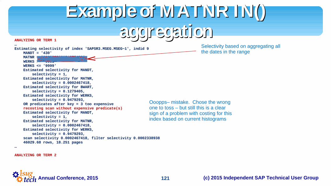
121Annual Conference, 2015 (c) 2015 Independent SAP Technical User Group
Example of MATNR IN() Example of MATNR IN() aggregationaggregation
ANALYZING OR TERM 1…Estimating selectivity of index 'SAPSR3.MSEG.MSEG~1', indid 9 MANDT = '430' MATNR = '000000000081075462' WERKS >= '0001' WERKS <= '9999' Estimated selectivity for MANDT, selectivity = 1, Estimated selectivity for MATNR, selectivity = 0.0002467418, Estimated selectivity for BWART, selectivity = 0.1279405, Estimated selectivity for WERKS, selectivity = 0.9479293, OR predicates after key = 3 too expensive recosting scan without expensive predicate(s) Estimated selectivity for MANDT, selectivity = 1, Estimated selectivity for MATNR, selectivity = 0.0002467418, Estimated selectivity for WERKS, selectivity = 0.9479293, scan selectivity 0.0002467418, filter selectivity 0.0002338938 46029.68 rows, 18.251 pages…
ANALYZING OR TERM 2
Selectivity based on aggregating all the dates in the range
Ooopps– mistake. Chose the wrong one to toss – but still this is a clear sign of a problem with costing for this index based on current histograms

122Annual Conference, 2015 (c) 2015 Independent SAP Technical User Group
Checking MSEG.BWARTChecking MSEG.BWARTStatistics for column: BWARTLast update of column statistics: Feb 2 2014 6:04:56:553AMRange cell density: 0.0006569891717182Total density: 0.1215260424316312Range selectivity: Default Used (0.33)In between selectivity: Default Used (0.25)Unique range values: 0.0001165239721073Unique total values: 0.0055555555555556Average column width: 3.0000000000000000Statistics version: 4
…
Step Weight Value
1 0.00000000 < '101' 2 0.10056020 = '101' 3 0.00157263 < '251' 4 0.01216128 = '251' 5 0.00009265 < '261' 6 0.12339991 = '261'… 29 0.00221821 < '555' 30 0.00215850 = '555' 31 0.00125471 < '562' 32 0.00155413 = '562'… 38 0.04804344 = '633' 39 0.00002823 < '641' 40 0.02545700 = '641' 41 0.00183529 < '657'…
Orders of magnitude diff tells us that there is some huge skew in the values….
Skew is not as bad as it could be – unfortunately, we are after one of the skewed values…and likely 12%+ of table
AND T_01."BWART" IN ( '101' , '561' , '643' , '641' )
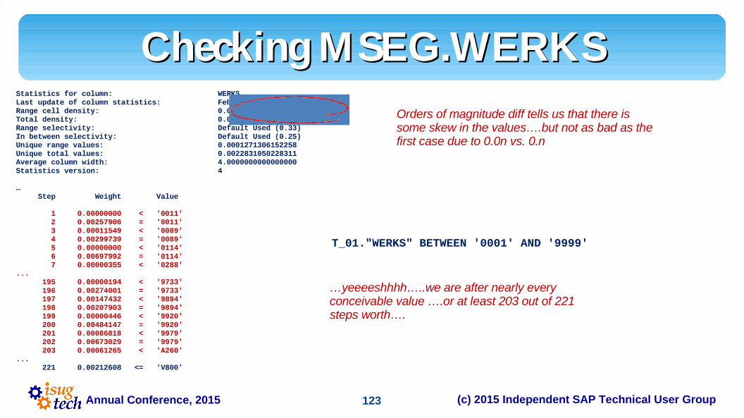
123Annual Conference, 2015 (c) 2015 Independent SAP Technical User Group
Checking MSEG.WERKSChecking MSEG.WERKSStatistics for column: WERKSLast update of column statistics: Feb 2 2014 6:04:56:553AMRange cell density: 0.0006185687162727Total density: 0.0214602987886209Range selectivity: Default Used (0.33)In between selectivity: Default Used (0.25)Unique range values: 0.0001271306152258Unique total values: 0.0022831050228311Average column width: 4.0000000000000000Statistics version: 4
… Step Weight Value
1 0.00000000 < '0011' 2 0.00257906 = '0011' 3 0.00011549 < '0089' 4 0.00299739 = '0089' 5 0.00000000 < '0114' 6 0.00697992 = '0114' 7 0.00000355 < '0288'... 195 0.00000194 < '9733' 196 0.00274001 = '9733' 197 0.00147432 < '9894' 198 0.00207903 = '9894' 199 0.00000446 < '9920' 200 0.00484147 = '9920' 201 0.00086818 < '9979' 202 0.00673029 = '9979' 203 0.00061265 < 'A260'... 221 0.00212608 <= 'V800'
Orders of magnitude diff tells us that there is some skew in the values….but not as bad as the first case due to 0.0n vs. 0.n
…yeeeeshhhh…..we are after nearly every conceivable value ….or at least 203 out of 221 steps worth….
T_01."WERKS" BETWEEN '0001' AND '9999'

124Annual Conference, 2015 (c) 2015 Independent SAP Technical User Group
Uh Oh…a Bit UglyUh Oh…a Bit UglyFrom the individual columns
q MATNR = 24% of tableq BWART = 12% of tableq WERKS = 99% of table
Sooo…q We could be looking for any where from 12% to 24% of tableq …or possibly less depending on the combinations of
MATNR+BWART…best bet would be to look at the multi-column densities
q But the reality is we really don’t have any other real index choice
q However, we still need to determine whether a tablescan would be betterü …especially if our cluster ratio for that index was a tad
ugly

125Annual Conference, 2015 (c) 2015 Independent SAP Technical User Group
What did we learnWhat did we learnWe picked the correct index…
q …inspite of the predicates weren’t so hot…soooo…any index with decent MATNR costing will likely be used
q Which index is cheaper? MSEG~0 MANDT, MBLNR, MJAHR, ZEILE nonclustered, unique ... MSEG~A MANDT, AUFNR nonclustered ... MSEG~R MANDT, RSNUM nonclustered ... MSEG~S SMBLN, SJAHR, SMBLP nonclustered ... MSEG~M MANDT, MATNR, WERKS, LGORT, BWART, SOBKZ nonclustered ... MSEG~Z03 MANDT, WERKS, BWART, LGORT nonclustered ... MSEG~Z02 MANDT, MATNR, CHARG, HSDAT, VFDAT nonclustered ... MSEG~1 MANDT, MATNR, BWART, WERKS nonclustered
q MSEG~1 wins likely based on IO costing as is smaller index….we got lucky?ü But an index such as {MANDT,MATNR,LGORT} may have
been used instead if it existed ü Using prepared statements/statement cache, subsequent
executions that had more usable BWART or WERKS values/ranges would suffer….ughhh

126Annual Conference, 2015 (c) 2015 Independent SAP Technical User Group
A very similar queryA very similar querySELECT T_00."MBLNR" ,T_00."MJAHR" ,T_01."MATNR" ,T_01."WERKS" ,T_01."BWART"
,T_01."SHKZG" ,T_01."MENGE" FROM "MKPF" T_00
INNER JOIN "MSEG" T_01 ON T_01."MANDT" = ? AND T_00."MBLNR" = T_01."MBLNR" AND T_00."MJAHR" = T_01."MJAHR"
WHERE T_00."MANDT" = ? AND T_00."BUDAT" BETWEEN ? AND ? AND T_01."MATNR" IN ( ? , ? , ? , ? , ? , ? , ? , ?
, ? , ? , ? , ? , ? , ? , ? , ? ) AND T_01."WERKS" IN ( ? , ? , ? , ? ) AND ( T_01."BWART" IN ( ? , ? , ? ) OR T_01."BWART" BETWEEN ? AND ? ) /* R3:ZCXXP015:987 T:MKPF M:430 */
16 params! 4 params! 3 params + range !

127Annual Conference, 2015 (c) 2015 Independent SAP Technical User Group
The Lava TreeThe Lava Tree==================== Lava Operator Tree ==================== Emit (VA = 8) r:161 er:2084 cpu: 7000 / MergeJoin Inner Join (VA = 7) r:161 er:2084 / \ Sort Sort (VA = 4) (VA = 6) r:6038 er:91527 r:1.418e+06 er:1.377e+06 l:32 el:247 l:2736 el:2162 p:4 ep:484 p:0 ep:4314 cpu: 1900 bufct: 24 cpu: 5600 bufct: 55 / / NestLoopJoin IndexScan Inner Join MKPF~Z03 (T_00) (VA = 3) (VA = 5) r:6038 er:91527 r:1.419e+06 er:1.377e+06 l:0 el:149438 l:41573 el:49684 p:0 ep:88824 p:2273 ep:8379/ \OrScan RestrictMax Rows: 4 (0)(0)(0)(4)(0)(VA = 0) (VA = 2)r:4 er:-1 r:6038 er:91527l:0 el:-1 /p:0 ep:-1 IndexScan MSEG~Z03 (T_01) (VA = 1) r:344336 er:91527 l:55015 el:149438 p:2868 ep:88824============================================================
WHOA!!!! …and SMJ….this is a bell ringer for bad bad bad
…and our row estimates are way way off….
Wrong index….

128Annual Conference, 2015 (c) 2015 Independent SAP Technical User Group
Delving into the ‘set option show’Delving into the ‘set option show’Estimating selectivity of index 'SAPSR3.MKPF.MKPF~Z03', indid 6 MANDT = '430' BUDAT >= '20131201' BUDAT <= '20131231' Estimated selectivity for MANDT, selectivity = 1, Estimated selectivity for BUDAT, selectivity = 0.02723849, scan selectivity 0.02723849, filter selectivity 0.02723849 1376633 rows, 507.0717 pages Data Row Cluster Ratio 0.9704043 Index Page Cluster Ratio 0.999693 Data Page Cluster Ratio 0.6074191 using index prefetch (size 128K I/O) Large IO selected: The number of leaf pages qualified is > MIN_PREFETCH pages in index cache 'default data cache' (cacheid 0) with LRU replacement
using table prefetch (size 128K I/O) Large IO selected: The number of leaf pages qualified is > MIN_PREFETCH pages in data cache 'default data cache' (cacheid 0) with LRU replacement Data Page LIO for 'MKPF~Z03' on table 'SAPSR3.MKPF' = 49174.02
Sooo…here is the problem….we have 16 MATNR values…most of which we have no stats on…all but the first is computed at 19 pages for a total of 288 pages (15*19.15+1=288)…and 691109 rows
…and that is just processing 1 side of the rest of the OR’s due to IN()
ANALYZING OR TERM 1…Estimating selectivity of index 'SAPSR3.MSEG.MSEG~1', indid 9 MATNR = 'MOR-CAIRO DC' MANDT = '430' Estimated selectivity for MANDT, selectivity = 1, Estimated selectivity for MATNR, Out of range histogram adjustment, selectivity = 4.423644e-06, scan selectivity 4.423644e-06, filter selectivity 4.423644e-06 825.3096 rows, 1 pages…
Index Competition for OR TERM with best candidate MSEG~1…ANALYZING OR TERM 16…Estimating selectivity of index 'SAPSR3.MSEG.MSEG~1', indid 9 MATNR = '000000000081186903' MANDT = '430' Estimated selectivity for MANDT, selectivity = 1, Estimated selectivity for MATNR, Out of range histogram adjustment, selectivity = 0.0002466606, scan selectivity 0.0002466606, filter selectivity 0.0002466606 46018.92 rows, 19.15122 pages…
Index Competition for OR TERM with best candidate MSEG~1
Statistics for column: MATNRLast update of column statistics: Feb 2 2014 6:04:56:553AMRange cell density: 0.0002466616441432Total density: 0.0002609528795212Range selectivity: Default Used (0.33)In between selectivity: Default Used (0.25)Unique range values: 0.0000043589934310Unique total values: 0.0000044236826273

129Annual Conference, 2015 (c) 2015 Independent SAP Technical User Group
……doing the IN() on WERKSdoing the IN() on WERKSANALYZING OR TERM 1…Estimating selectivity of index 'SAPSR3.MSEG.MSEG~1', indid 9 WERKS = 'A749' MANDT = '430' Estimated selectivity for MANDT, selectivity = 1, Estimated selectivity for MATNR, Out of range histogram adjustment, selectivity = 0.003704332, Estimated selectivity for WERKS, selectivity = 0.001792594, scan selectivity 0.003704332, filter selectivity 0.001270694 special or terms 16 691109.2 rows, 287.6117 pages Data Row Cluster Ratio 0.2232867 Index Page Cluster Ratio 0.9038212 Data Page Cluster Ratio 0.1132857 using index prefetch (size 128K I/O) Large IO selected: The number of leaf pages qualified is > MIN_PREFETCH pages in index cache 'default data cache' (cacheid 0) with LRU replacement
Index Competition for OR TERM with best candidate MSEG~M
3 of the 4 OR’s on WERKS IN () chose to do MSEG~Z03 …the first one chose MSEG~M ….none chose MSEG~1 which is what we thought…. The problem is the out of range histogram and the large number of IN() values is causing a costing problem ….running update stats with higher step count is a definite solution to try.
ANALYZING OR TERM 4…Estimating selectivity of index 'SAPSR3.MSEG.MSEG~Z03', indid 7 WERKS = '9781' MANDT = '430' Estimated selectivity for MANDT, selectivity = 1, Estimated selectivity for WERKS, selectivity = 0.0004913162, scan selectivity 0.0004913162, filter selectivity 0.0004913162 91663.8 rows, 34.06688 pages Data Row Cluster Ratio 0.774294 Index Page Cluster Ratio 0.9807813 Data Page Cluster Ratio 0.4206219 using index prefetch (size 128K I/O) Large IO selected: The number of leaf pages qualified is > MIN_PREFETCH pages in index cache 'default data cache' (cacheid 0) with LRU replacement
Estimating selectivity of index 'SAPSR3.MSEG.MSEG~1', indid 9 WERKS = '9781' MANDT = '430' Estimated selectivity for MANDT, selectivity = 1, Estimated selectivity for MATNR, Out of range histogram adjustment, selectivity = 0.003704332, Estimated selectivity for WERKS, selectivity = 0.0004913162, scan selectivity 0.003704332, filter selectivity 0.00131834 special or terms 16 691109.2 rows, 287.6117 pages… using index prefetch (size 128K I/O) Large IO selected: The number of leaf pages qualified is > MIN_PREFETCH pages in index cache 'default data cache' (cacheid 0) with LRU replacement
Index Competition for OR TERM with best candidate MSEG~Z03
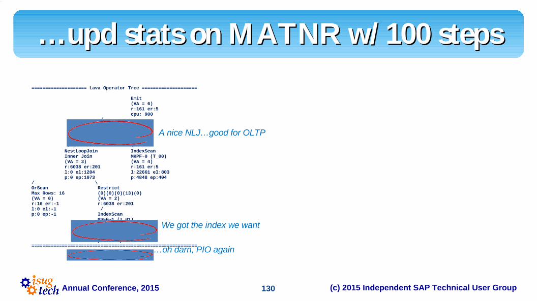
130Annual Conference, 2015 (c) 2015 Independent SAP Technical User Group
……upd stats on MATNR w/ 100 stepsupd stats on MATNR w/ 100 steps
==================== Lava Operator Tree ==================== Emit (VA = 6) r:161 er:5 cpu: 900 / NestLoopJoin Inner Join (VA = 5) r:161 er:5 / \ NestLoopJoin IndexScan Inner Join MKPF~0 (T_00) (VA = 3) (VA = 4) r:6038 er:201 r:161 er:5 l:0 el:1204 l:22661 el:803 p:0 ep:1073 p:4848 ep:404/ \OrScan RestrictMax Rows: 16 (0)(0)(0)(13)(0)(VA = 0) (VA = 2)r:16 er:-1 r:6038 er:201l:0 el:-1 /p:0 ep:-1 IndexScan MSEG~1 (T_01) (VA = 1) r:9510 er:201 l:7591 el:1204 p:1081 ep:1073============================================================
A nice NLJ…good for OLTP
We got the index we want
…oh darn, PIO again

131Annual Conference, 2015 (c) 2015 Independent SAP Technical User Group
Stop me if you’ve seen this before….Stop me if you’ve seen this before….Table: SAPSR3.MSEG (T_01) scan count 16, logical reads: (regular=7591 apf=0 total=7591),
physical reads: (regular=1019 apf=62 total=1081), apf IOs used=62Table: SAPSR3.MKPF (T_00) scan count 6038, logical reads: (regular=22661 apf=0 total=22661),
physical reads: (regular=4843 apf=5 total=4848), apf IOs used=1Total writes for this command: 0
Execution Time 9.Adaptive Server cpu time: 1005 ms. Adaptive Server elapsed time: 63278 ms.…1> 2> 3> select * from master..monProcessWaits where SPID=@@SPID order by WaitEventIDSPID InstanceIDKPID ServerUserID WaitEventIDWaits WaitTime ----------- ---------- ----------- ------------ ----------- ----------- ----------- 608 0 258409561 4 29 5862 61924 608 0 258409561 4 31 1 0 608 0 258409561 4 124 5 29 608 0 258409561 4 250 7 524 608 0 258409561 4 251 1 0
WaitEventID 29 = regular read;
WaitEventID 124=MASS reads (APF, etc.)
…do the math…63 secs elapsed and 62 secs in IO….where do you think the problem is?
..and our IO speed is 9ms per IO �

132Annual Conference, 2015 (c) 2015 Independent SAP Technical User Group
Oh, BTW…..from Oh, BTW…..from monCachedObjectmonCachedObject
Not helping us as it is driving our desired table out of cache

133Annual Conference, 2015 (c) 2015 Independent SAP Technical User Group
The lessonThe lessonFor fairly distinct columns…
q Increasing the number of steps helps reduce the number of rows estimated for IN() clauses as they are cumulative
q You may need to run update stats more often on just that column to prevent out of range histograms
For cols with high skewq Consider using sp_modifystats to reduce densities by 100 or
1000ü May not help queries without joins, but queries with joins
may benefit (test and see)ü If it doesn’t just re-update stats and it wipes out the
modified statsNot all slowness is due to optimization picking bad plan…slow disks are
slow disks

(c) 2015 Independent SAP Technical User GroupAnnual Conference, 2015
CONTROLLING OPTIMIZATIONCONTROLLING OPTIMIZATIONThings you can do when desperate….

135Annual Conference, 2015 (c) 2015 Independent SAP Technical User Group
Methods of Controlling Methods of Controlling OptimizationOptimization
Some we already have seenq Increasing histogram stepsq Adding inferred/implicit range boundariesq Eliminate “conditional” where clausesq Eliminate unnecessary operators (e.g. scalar aggregates
vs. group by)Some more direct methods
q Manual stats adjustmentq Sp_modifystatsq Sp_chgattributeq Sp_configure ‘resource granularity’

136Annual Conference, 2015 (c) 2015 Independent SAP Technical User Group
Manual Stats AdjustmentManual Stats AdjustmentWhen it works:
q Low cardinality/volatile columns such as status, type, etc.
Process:q Extract stats via optdiagq Modify low cardinality stats
ü Remember to adjust step count
q Reload using optdiag as simulated statsü Test queries with simulated stats
q Reload as real stats with optdiag

137Annual Conference, 2015 (c) 2015 Independent SAP Technical User Group
Manual Stats: before & afterManual Stats: before & afterStatistics for column: "STATUS"Last update of column statistics: Mar 18 2013 3:00:00:720PM
Range cell density: 0.0008480622450765 Total density: 0.9760966822891640 Range selectivity: default used (0.33) In between selectivity: default used (0.25) Unique range values: 0.0008480622450765 Unique total values: 0.3333333333333333 Average column width: 1.0000000000000000 Statistics version: 4
Histogram for column: "STATUS"Column datatype: varchar(3)Requested step count: 20Actual step count: 4Sampling Percent: 0Tuning Factor: 20Out of range Histogram Adjustment is DEFAULT.Low Domain Hashing.Sticky step count.Sticky partial_hashing.
Step Weight Value
1 0.00000000 < "C" 2 0.98791176 = "C" 3 0.00084806 < "T" 4 0.01124019 = "T"
Add some steps we want
Statistics for column: "STATUS"Last update of column statistics: Mar 18 2013 3:00:00:720PM
Range cell density: 0.0008000000000000 Total density: 0.9204652800000000 Range selectivity: default used (0.33) In between selectivity: default used (0.25) Unique range values: 0.0008000000000000 Unique total values: 0.0833333333333333 Average column width: 1.0000000000000000 Statistics version: 4
Histogram for column: "STATUS"Column datatype: varchar(3)Requested step count: 20Actual step count: 9Sampling Percent: 0Tuning Factor: 20Out of range Histogram Adjustment is DEFAULT.Low Domain Hashing.Sticky step count.Sticky partial_hashing.
Step Weight Value
1 0.00000000 < "C" 2 0.95920000 = "C" 3 0.00000000 < "F" 4 0.01000000 = "F" 5 0.00000000 < "P" 6 0.01000000 = "P" 7 0.00080000 < "T" 8 0.01000000 = "T" 9 0.01000000 <= "Z"
Set to 1.0 – sum(others)
Round for easier math
Adjust for distinct values in domain
Adjust
Sum(weight^2)
<min(weight)
<min(weight)
Add to prevent out of range statsMake sure sum(weights) = 1.0 precisely

138Annual Conference, 2015 (c) 2015 Independent SAP Technical User Group
Sp_modifystatsSp_modifystatsSyntax:
q Typical syntax sp_modifystats [database].[owner].table_name, {"column_group" | "all"}, MODIFY_DENSITY, {range | total},{absolute | factor},"value"
q Alternative: sp_modifystats [database].[owner].table_name, column_name | null, REMOVE_SKEW_FROM_DENSITY | REMOVE_STICKINESS
Use cases:q Note: not persistent – next update statistics resets to ASE compute
valueq Best example is when one of the total density values is highly skewedq If skewed column is not part of a join, use first syntax and adjust
total/absolute exec sp_modifystats 'SAPSR3.COEP', 'KSTAR','MODIFY_DENSITY',
'total','absolute','0.0006'
q If skewed column is part of join key, use second syntax with REMOVE_SKEW…
exec sp_modifystats 'SAPSR3.COEP','OBJNR', REMOVE_SKEW_FROM_DENSITY

139Annual Conference, 2015 (c) 2015 Independent SAP Technical User Group
Sp_chgattributeSp_chgattributeSp_chgattribute ‘opt concurrency threshold’
q Interesting definition for a value of -1 specifies the table size, in pages, at which access to a data-only-locked table should begin optimizing
for reducing I/O, rather than for concurrency. If the table is smaller than the number of pages specified by concurrency_opt_threshold, the query is optimized for concurrency by always using available indexes; if the table is larger than the number of pages specified by concurrency_opt_threshold, the query is optimized for I/O instead. Valid values are -1 to 32767. Setting the value to 0 disables concurrency optimization. Use -1 to enforce concurrency optimization for tables larger than 32767 pages. The default is 15 pages.
q What it really means is ASE will use rules (vs. cost) optimizationü Attempt to use best matching index for predicates
Use cases:q Very volatile tables
ü Not just a single column (e.g. status) …but the rowsü For example a workflow queue table
q Force index use despite data skewü As an alternative to sp_modifystats

140Annual Conference, 2015 (c) 2015 Independent SAP Technical User Group
Sp_configure ‘resource granularity’Sp_configure ‘resource granularity’Another bad default config?
q Started in ASE 15.0 – default to 10%By the docs
q specify the percentage of total memory that Adaptive Server can allocate to a single query
q If max resource granularity is set low, many hash- and sort-based operators cannot be chosen. max resource granularity also affects the scheduling algorithm
Translation in Englishq Sort/Hash based operations require a lot of memory
ü Memory in data cache for actual sortingü Memory in proc cache for aux keep buffers (track sort pages)
q By reducing memory allowed to use, ASE may not pick SMJ as often
Better technique? � custom optimization level (ASE 15.7 sp100+)

141Annual Conference, 2015 (c) 2015 Independent SAP Technical User Group
Setting a custom optimization levelSetting a custom optimization level-- pick the default starting level you wantset plan optlevel ase_current-- pick the default optgoalset plan optgoal allrows_mix-- enable or disable any optimization criteriaset merge_join 0-- saveexec sp_optgoal 'sap_oltp', 'save'go
-- to useset plan optgoal sap_oltpgo
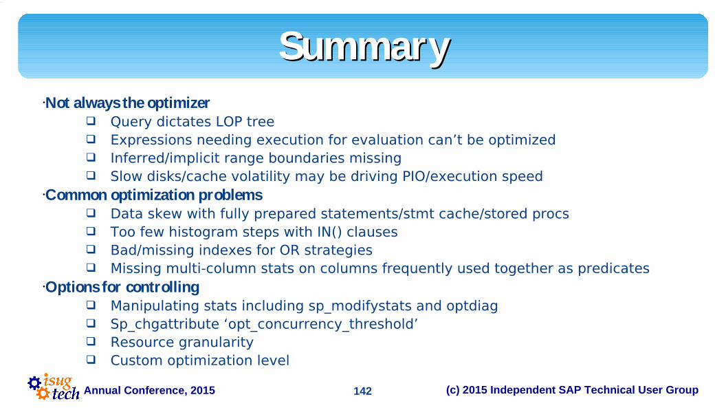
142Annual Conference, 2015 (c) 2015 Independent SAP Technical User Group
SummarySummaryNot always the optimizer
q Query dictates LOP treeq Expressions needing execution for evaluation can’t be optimizedq Inferred/implicit range boundaries missingq Slow disks/cache volatility may be driving PIO/execution speed
Common optimization problemsq Data skew with fully prepared statements/stmt cache/stored procsq Too few histogram steps with IN() clausesq Bad/missing indexes for OR strategiesq Missing multi-column stats on columns frequently used together as predicates
Options for controllingq Manipulating stats including sp_modifystats and optdiagq Sp_chgattribute ‘opt_concurrency_threshold’ q Resource granularityq Custom optimization level

(c) 2015 Independent SAP Technical User GroupAnnual Conference, 2015
Questions and Answers Questions and Answers

(c) 2015 Independent SAP Technical User GroupAnnual Conference, 2015
Thank You for Attending Thank You for Attending
Please complete your session Please complete your session feedback form feedback form