the return/volatility trade-off of distressed …people.stern.nyu.edu/ealtman/the...

THE JOURNAL OF PORTFOLIO MANAGEMENT 69WINTER 2014

The Return/Volatility Trade-Off of Distressed Corporate Debt PortfoliosEDWARD I. ALTMAN, JOSÉ F. GONZÁLEZ-HERES, PING CHEN, AND STEVEN S. SHIN

EDWARD I. ALTMAN

is the Max L. Heine Professor of Finance at the Stern School of Business at New York University in New York, [email protected]

JOSÉ F. GONZÁLEZ-HERES

is a managing director and portfolio manager for the Fund of Hedge Funds portfolios at Morgan Stanley AIP and a mem - ber of its investment committee in West Conshohocken, [email protected]

PING CHEN

is a research analyst for the Fund of Hedge Funds portfolios at Morgan Stanley AIP in West Conshohocken, [email protected]

STEVEN S. SHIN

is a research analyst for the Fund of Hedge Funds portfolios at Morgan Stanley AIP in West Conshohocken, [email protected]

Capita l a s set-pr ic ing model (CAPM)1 theory suggests that higher equity volatility invest-ments should lead to higher

expected returns. This article does not attempt to challenge CAPM theory beyond this risk/return relationship. When the theory is applied to a portfolio of distressed corporate bonds, our empirical analysis can either support or refute the theory, depending on whether or not the effect of systematic volatility of the high-yield corporate bond market is taken into consideration. The anal-ysis revolves around segmenting the distressed component of the high-yield market into four distinct bond portfolios, based on a quartile ranking of their realized option-adjusted spread (OAS) volatility six months prior to technically becoming distressed.2 We define volatility as the monthly standard deviation of the OAS. The analysis is performed in both a time-independent (distressed securi-ties from different dates are re-aligned such that t = 0 is their f irst instance of distress) and time-dependent (based on the historical occurrence of distress over continuous time) fashion, to provide both theoretical and prac-tical perspectives to the analysis. We define the four portfolios as f irst quartile, or LO VOL; second quartile; third quartile; and, “fourth quartile, or HI VOL). We concen-trate the discussion of our f indings on the

lowest- and highest-volatility portfolios, LO VOL and HI VOL, respectively.

We hypothesize that over the long term, lower-volatility distressed securities should generate improved returns, relative to higher-volatility distressed securities. The intuition of our hypothesis is based on empirical research by González-Heres et al. [2010], who found that distressed securities that eventually defaulted exhibited approximately 2.5 times the OAS volatility of distressed securities that did not default.

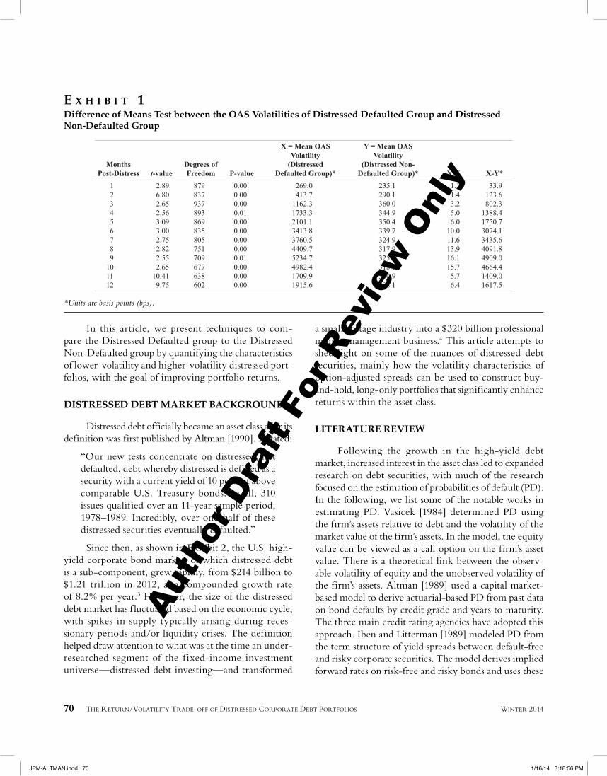
Exhibit 1 shows the results of a differ-ence of means test between distressed securi-ties that defaulted (distressed Defaulted group) versus those that did not default (distressed Non-Defaulted group) over the analysis period of July 1997 to December 2012. We calculate the difference of the mean OAS volatilities between the two groups on a monthly basis, starting with the first instance of the security becoming distressed. The test clearly shows strong statistically signifi-cant differences between the average spread volatility of the two groups. In particular, after a group’s second month in distress, we observe a materially higher statistical differ-ence (t-value of 6.80), which occurs early in the distress evolution process and thus is ben-eficial in identifying the two distinct groups from a practical perspective.

JPM-ALTMAN.indd 69JPM-ALTMAN.indd 69 1/16/14 3:18:56 PM1/16/14 3:18:56 PM

Auth

or D

raft

For R

evie

w O

nly

70 THE RETURN/VOLATILITY TRADE-OFF OF DISTRESSED CORPORATE DEBT PORTFOLIOS WINTER 2014

In this article, we present techniques to com-pare the Distressed Defaulted group to the Distressed Non-Defaulted group by quantifying the characteristics of lower-volatility and higher-volatility distressed port-folios, with the goal of improving portfolio returns.

DISTRESSED DEBT MARKET BACKGROUND

Distressed debt officially became an asset class after its definition was first published by Altman [1990]. It stated:

“Our new tests concentrate on distressed, not defaulted, debt whereby distressed is defined as a security with a current yield of 10 percent above comparable U.S. Treasury bonds. In all, 310 issues qualified over an 11-year sample period, 1978–1989. Incredibly, over one-half of these distressed securities eventually defaulted.”

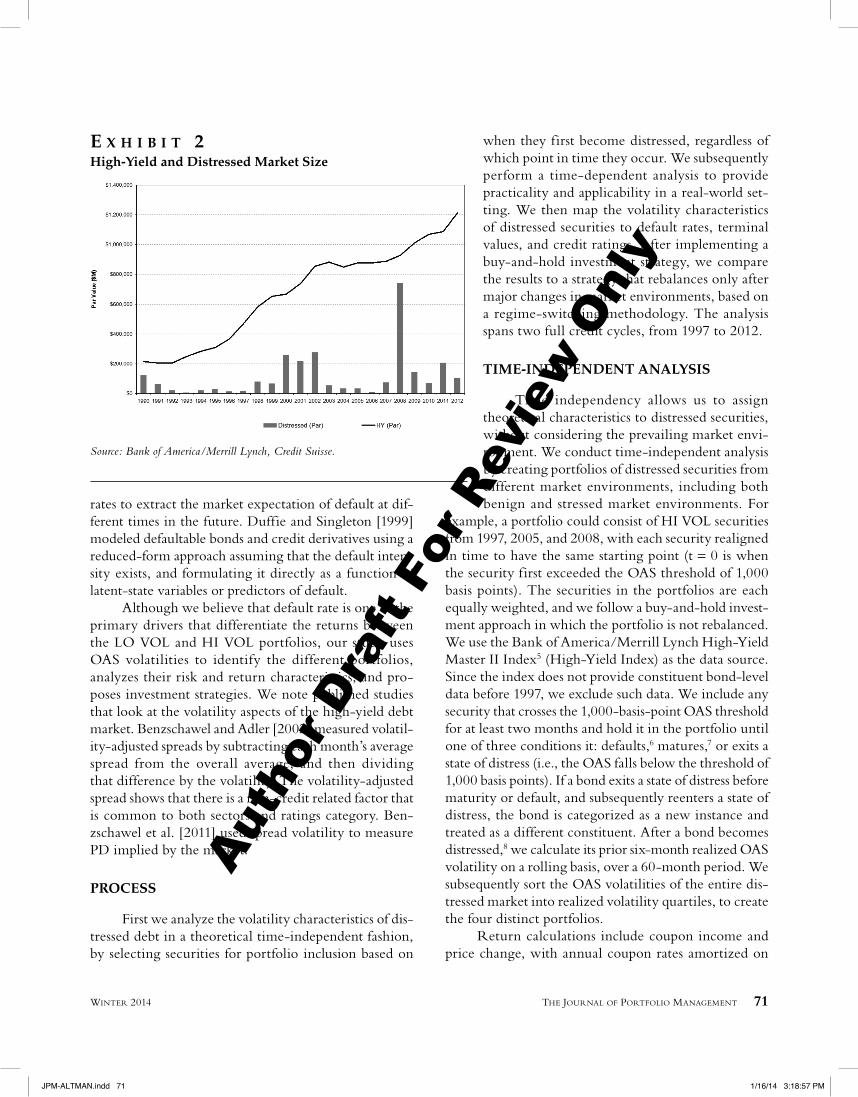
Since then, as shown in Exhibit 2, the U.S. high-yield corporate bond market, of which distressed debt is a sub-component, grew rapidly, from $214 billion to $1.21 trillion in 2012, at a compounded growth rate of 8.2% per year.3 However, the size of the distressed debt market has f luctuated based on the economic cycle, with spikes in supply typically arising during reces-sionary periods and/or liquidity crises. The definition helped draw attention to what was at the time an under-researched segment of the f ixed-income investment universe—distressed debt investing—and transformed

a small cottage industry into a $320 billion professional money management business.4 This article attempts to shed light on some of the nuances of distressed-debt securities, mainly how the volatility characteristics of option-adjusted spreads can be used to construct buy-and-hold, long-only portfolios that significantly enhance returns within the asset class.

LITERATURE REVIEW

Following the growth in the high-yield debt market, increased interest in the asset class led to expanded research on debt securities, with much of the research focused on the estimation of probabilities of default (PD). In the following, we list some of the notable works in estimating PD. Vasicek [1984] determined PD using the firm’s assets relative to debt and the volatility of the market value of the firm’s assets. In the model, the equity value can be viewed as a call option on the firm’s asset value. There is a theoretical link between the observ-able volatility of equity and the unobserved volatility of the firm’s assets. Altman [1989] used a capital market-based model to derive actuarial-based PD from past data on bond defaults by credit grade and years to maturity. The three main credit rating agencies have adopted this approach. Iben and Litterman [1989] modeled PD from the term structure of yield spreads between default-free and risky corporate securities. The model derives implied forward rates on risk-free and risky bonds and uses these

*Units are basis points (bps).

E X H I B I T 1Difference of Means Test between the OAS Volatilities of Distressed Defaulted Group and Distressed Non-Defaulted Group


Auth

or D

raft

For R

evie

w O

nly


rates to extract the market expectation of default at dif-ferent times in the future. Duffie and Singleton [1999] modeled defaultable bonds and credit derivatives using a reduced-form approach assuming that the default inten-sity exists, and formulating it directly as a function of latent-state variables or predictors of default.

Although we believe that default rate is one of the primary drivers that differentiate the returns between the LO VOL and HI VOL portfolios, our study uses OAS volatilities to identify the different portfolios, analyzes their risk and return characteristics, and pro-poses investment strategies. We note published studies that look at the volatility aspects of the high-yield debt market. Benzschawel and Adler [2002] measured volatil-ity-adjusted spreads by subtracting each month’s average spread from the overall average, and then dividing that difference by the volatility. The volatility-adjusted spread shows that there is a non-credit related factor that is common to both sectors and ratings category. Ben-zschawel et al. [2011] used spread volatility to measure PD implied by the market.

PROCESS

First we analyze the volatility characteristics of dis-tressed debt in a theoretical time-independent fashion, by selecting securities for portfolio inclusion based on

when they first become distressed, regardless of which point in time they occur. We subsequently perform a time-dependent analysis to provide practicality and applicability in a real-world set-ting. We then map the volatility characteristics of distressed securities to default rates, terminal values, and credit ratings. After implementing a buy-and-hold investment strategy, we compare the results to a strategy that rebalances only after major changes in market environments, based on a regime-switching methodology. The analysis spans two full credit cycles, from 1997 to 2012.

TIME-INDEPENDENT ANALYSIS

Time independency allows us to assign theoretical characteristics to distressed securities, without considering the prevailing market envi-ronment. We conduct time-independent analysis by creating portfolios of distressed securities from different market environments, including both benign and stressed market environments. For

example, a portfolio could consist of HI VOL securities from 1997, 2005, and 2008, with each security realigned in time to have the same starting point (t = 0 is when the security first exceeded the OAS threshold of 1,000 basis points). The securities in the portfolios are each equally weighted, and we follow a buy-and-hold invest-ment approach in which the portfolio is not rebalanced. We use the Bank of America/Merrill Lynch High-Yield Master II Index5 (High-Yield Index) as the data source. Since the index does not provide constituent bond-level data before 1997, we exclude such data. We include any security that crosses the 1,000-basis-point OAS threshold for at least two months and hold it in the portfolio until one of three conditions it: defaults,6 matures,7 or exits a state of distress (i.e., the OAS falls below the threshold of 1,000 basis points). If a bond exits a state of distress before maturity or default, and subsequently reenters a state of distress, the bond is categorized as a new instance and treated as a different constituent. After a bond becomes distressed,8 we calculate its prior six-month realized OAS volatility on a rolling basis, over a 60-month period. We subsequently sort the OAS volatilities of the entire dis-tressed market into realized volatility quartiles, to create the four distinct portfolios.

Return calculations include coupon income and price change, with annual coupon rates amortized on

Source: Bank of America/Merrill Lynch, Credit Suisse.

E X H I B I T 2High-Yield and Distressed Market Size


Auth

or D

raft

For R

evie

w O

nly


a monthly basis from the time a bond first enters a state of distress. Cumulative returns are calculated over a 60-month period, after a bond first enters a state of dis-tress, and are used to compare the relative performance of the four portfolios. Time-independent analysis allows us to ascertain the respective portfolios’ risk and return characteristics and test CAPM theoretical expectations.

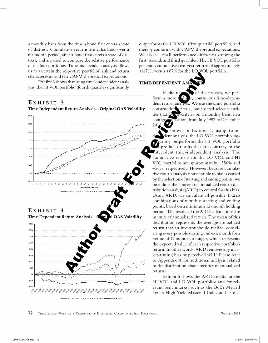
Exhibit 3 shows that using time-independent anal-ysis, the HI VOL portfolio (fourth quartile) significantly

outperforms the LO VOL (first quartile) portfolio, and thereby conforms with CAPM theoretical expectations. We also see small performance differentials among the first, second, and third quartiles. The HI VOL portfolio generates cumulative five-year returns of approximately +117%, versus +87% for the LO VOL portfolio.

TIME-DEPENDENT ANALYSIS

In the next step of the process, we per-form a more realistic, continuous time-depen-dent return analysis. We use the same portfolio construction criteria, but instead select securi-ties that fit the criteria on a monthly basis, in a contiguous fashion, from July 1997 to December 2012.

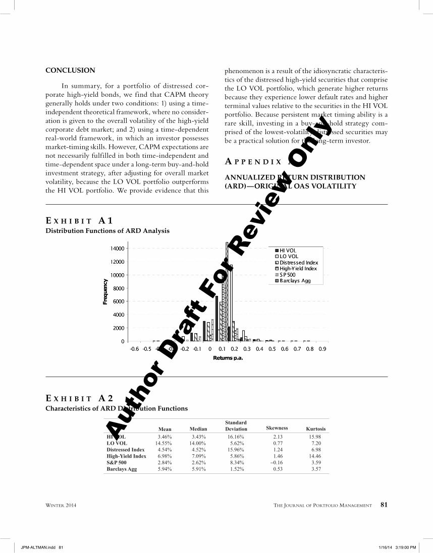
As shown in Exhibit 4, using time- dependent analysis, the LO VOL portfolio sig-nif icantly outperforms the HI VOL portfolio and produces results that are contrary to the antecedent time-independent analysis. The cumulative returns for the LO VOL and HI VOL portfolios are approximately +356% and −56%, respectively. However, because cumula-tive return analysis is susceptible to biases caused by the selection of starting and ending points, we introduce the concept of annualized return dis-tribution analysis (ARD) to control for this bias. Using ARD, we calculate all possible 15,225 combinations of monthly starting and ending points, based on a minimum 12-month holding period. The results of the ARD calculations are in units of annualized return. The mean of this distribution represents the average annualized return that an investor should realize, consid-ering every possible starting and exit month for a period of 12 months or longer, which represents the expected value of each respective portfolio’s return. In other words, ARD removes any mar-ket-timing bias or perceived skill.9 Please refer to Appendix A for additional analysis related to the distribution characteristics of annualized returns.

Exhibit 5 shows the ARD results for the HI VOL and LO VOL portfolios and for rel-evant benchmarks, such as the BofA Merrill Lynch High-Yield Master II Index and its dis-

E X H I B I T 3Time-Independent Return Analysis—Original OAS Volatility

E X H I B I T 4Time-Dependent Return Analysis—Original OAS Volatility


Auth

or D

raft

For R

evie

w O

nly


tressed sub-index (“Distressed Index”).10 The results are consistent with our hypothesis, because the mean return value of the LO VOL portfolio outperforms that of the HI VOL portfolio by 12.22 percentage points. Additionally, the LO VOL portfolio also outperforms the High-Yield Index and Distressed Index by 3.94 per-centage points and 6.38 percentage points, respectively. These results contradict the time-independent analysis and support our hypothesis that over the long term, lower-volatility distressed securities should outperform higher-volatility securities, because higher volatility securities should experience higher default rates. We investigate the default characteristics from a volatility perspective in the next section.

DEFAULT RATES AND TERMINAL VALUES

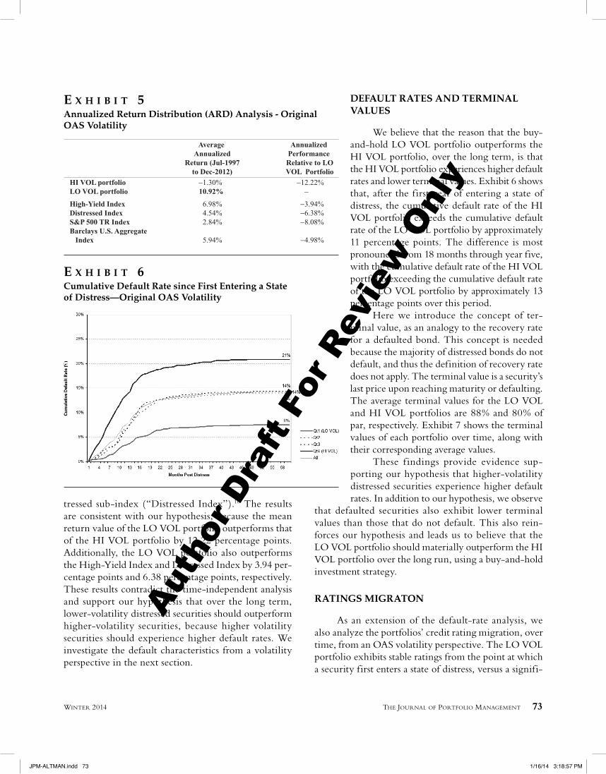
We believe that the reason that the buy-and-hold LO VOL portfolio outperforms the HI VOL portfolio, over the long term, is that the HI VOL portfolio experiences higher default rates and lower terminal values. Exhibit 6 shows that, after the first year of entering a state of distress, the cumulative default rate of the HI VOL portfolio exceeds the cumulative default rate of the LO VOL portfolio by approximately 11 percentage points. The difference is most pronounced from 18 months through year five, with the cumulative default rate of the HI VOL portfolio exceeding the cumulative default rate of the LO VOL portfolio by approximately 13 percentage points over this period.

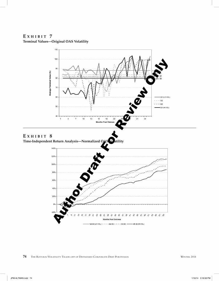
Here we introduce the concept of ter-minal value, as an analogy to the recovery rate for a defaulted bond. This concept is needed because the majority of distressed bonds do not default, and thus the definition of recovery rate does not apply. The terminal value is a security’s last price upon reaching maturity or defaulting. The average terminal values for the LO VOL and HI VOL portfolios are 88% and 80% of par, respectively. Exhibit 7 shows the terminal values of each portfolio over time, along with their corresponding average values.

These f indings provide evidence sup-porting our hypothesis that higher-volatility distressed securities experience higher default rates. In addition to our hypothesis, we observe

that defaulted securities also exhibit lower terminal values than those that do not default. This also rein-forces our hypothesis and leads us to believe that the LO VOL portfolio should materially outperform the HI VOL portfolio over the long run, using a buy-and-hold investment strategy.

RATINGS MIGRATON

As an extension of the default-rate analysis, we also analyze the portfolios’ credit rating migration, over time, from an OAS volatility perspective. The LO VOL portfolio exhibits stable ratings from the point at which a security first enters a state of distress, versus a signifi-

E X H I B I T 5Annualized Return Distribution (ARD) Analysis - Original OAS Volatility

E X H I B I T 6Cumulative Default Rate since First Entering a State of Distress—Original OAS Volatility


Auth

or D

raft

For R

evie

w O

nly


E X H I B I T 7Terminal Values—Original OAS Volatility

E X H I B I T 8Time-Independent Return Analysis—Normalized OAS Volatility


Auth

or D

raft

For R

evie

w O

nly


cant deterioration in credit quality during the first 12 months for the HI VOL portfolio. We also f ind that the HI VOL portfolio is generally comprised of a larger proportion of lower quality, CCC-C-rated securities, which are associated with higher default rates. (Please refer to Appendix B.)

NORMALIZING FOR MARKET VOLATILITY

It appears that in a theoretical (time-independent) world, over the long term, a buy-and-hold investment strategy consisting of a portfolio of the highest-vola-tility distressed corporate debt securities outperforms a portfolio of the lowest-volatility securities. How-ever, in a real-world (time-dependent) environment, a lower-volatility, buy-and-hold portfolio outperforms its higher volatility counterpart.

What drives this contradiction in results? Using time-independent analysis, we f ind that the HI VOL portfolio is made up almost entirely of securities from several dislocated markets (i.e., 1998, 2002, and 2008). This suggests that if an investor possesses market-timing skills, he is better off investing in the HI VOL portfolio, particularly after market dislocations. Rather than following a buy-and-hold investment approach,

portfolios should be rebalanced after market disloca-tions, overweighting the highest-volatility securities.

We believe that this contradiction in results can be attributed to the effect of overall high-yield corpo-rate bond market volatility (market volatility), which obscures the idiosyncratic volatility properties of indi-vidual distressed securities.

After conducting the same analysis, this time controlling for overall market volatility, we observe consistent results both in time-independent and time-dependent space, with the LO VOL portfolio outper-forming the HI VOL portfolio. (See Exhibits 8 and 9.) We control for market volatility by normalizing each individual bond’s OAS volatility by the market’s overall volatility. We accomplish normalization by dividing an individual bond’s trailing six-month realized vola-tility by the average realized volatility of the high-yield market over the same time period. By controlling for the volatility of the high-yield bond market, we remove systematic volatility effects and can thus analyze the idiosyncratic volatility properties of each individual dis-tressed security. This adjustment is important because, unless the data is normalized, the HI VOL portfolio is dominated by securities that only appear during the most volatile market environments, and thus the

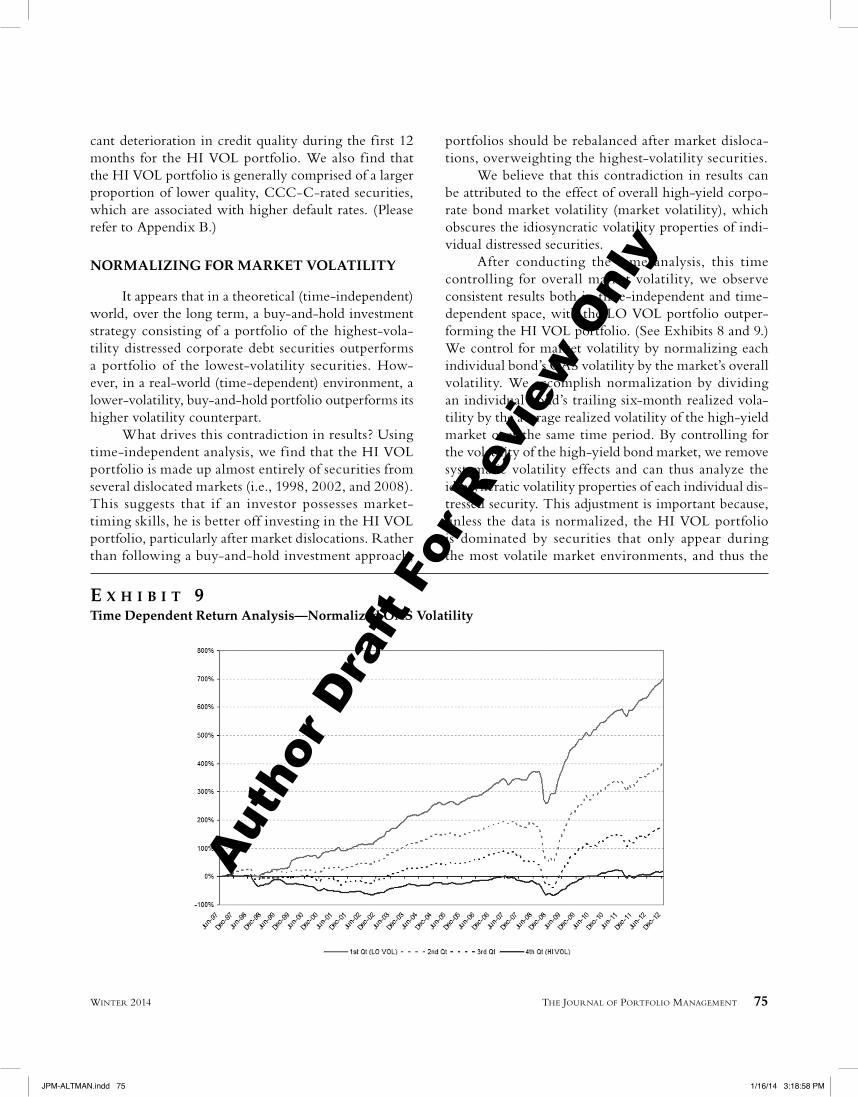
E X H I B I T 9Time Dependent Return Analysis—Normalized OAS Volatility


Auth

or D

raft

For R

evie

w O

nly


analysis provides little insight into an individual bond’s characteristics under heterogeneous market conditions. Normalization ensures that the HI VOL and LO VOL portfolios include only the highest- and lowest-volatility securities available at a coterminous point in time, over the diverse market volatility conditions covered by the analysis period.

After performing time-independent analysis using the normalized approach, the LO VOL portfolio consis-tently outperforms the HI VOL portfolio by a margin ranging from 17 to 47 percentage points of cumulative return. The effect is most pronounced 18 to 24 months

after a security f irst becomes distressed, with cumu-lative outperformance of 45 percentage points. (See Exhibit 8.) Therefore, in order to improve long-term returns using a buy-and-hold strategy, it is necessary to select the lowest-volatility securities that are available in the then-current market (i.e., controlling for overall market volatility) without relying on market-timing skills.

Next we analyze returns in a time-dependent fashion (Exhibit 9). We perform ARD analysis to elimi-nate entry and exit biases. Exhibit 10 shows that the LO VOL portfolio outperforms the HI VOL portfolio by 11.09 percentage points. The LO VOL portfolio also outperforms the High-Yield Index and the Distressed Index by 7.57 percentage points and 10.02 percentage points, respectively. Comparing the non-normalized results (Exhibit 5) to the normalized results (Exhibit 10), we find that normalization improves average annualized returns by 3 to 5 percentage points for both the LO VOL and HI VOL portfolios. However, the outperformance of the LO VOL portfolio, relative to the HI VOL port-folio, is similar at 11 to 12 percentage points for each case. After introducing normalization into the analysis, we find results that are consistent with our hypothesis using both a time- independent and time-dependent framework, with the LO VOL portfolio outperforming the HI VOL portfolio.

E X H I B I T 1 0Annualized Return Distribution (ARD) Analysis—Normalized OAS Volatility

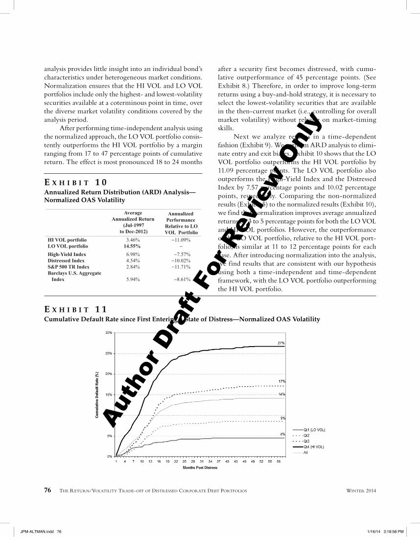
E X H I B I T 1 1Cumulative Default Rate since First Entering a State of Distress—Normalized OAS Volatility


Auth

or D

raft

For R

evie

w O

nly


Next, we analyze the default-rate characteristics under the normalized volatility framework. Exhibit 11 shows cumulative default rates for the volatility quartiles, after normalizing OAS spread volatility. After the first

year of entering a state of distress, the cumulative default rate of the HI VOL portfolio exceeds the cumulative default rate of the LO VOL portfolio by approximately 12 percentage points. The difference is most pronounced

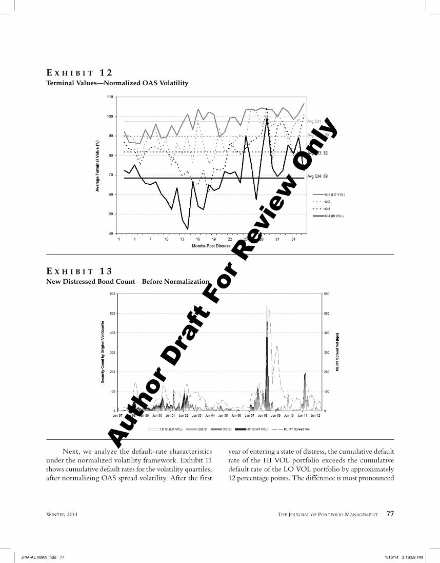
E X H I B I T 1 2Terminal Values—Normalized OAS Volatility

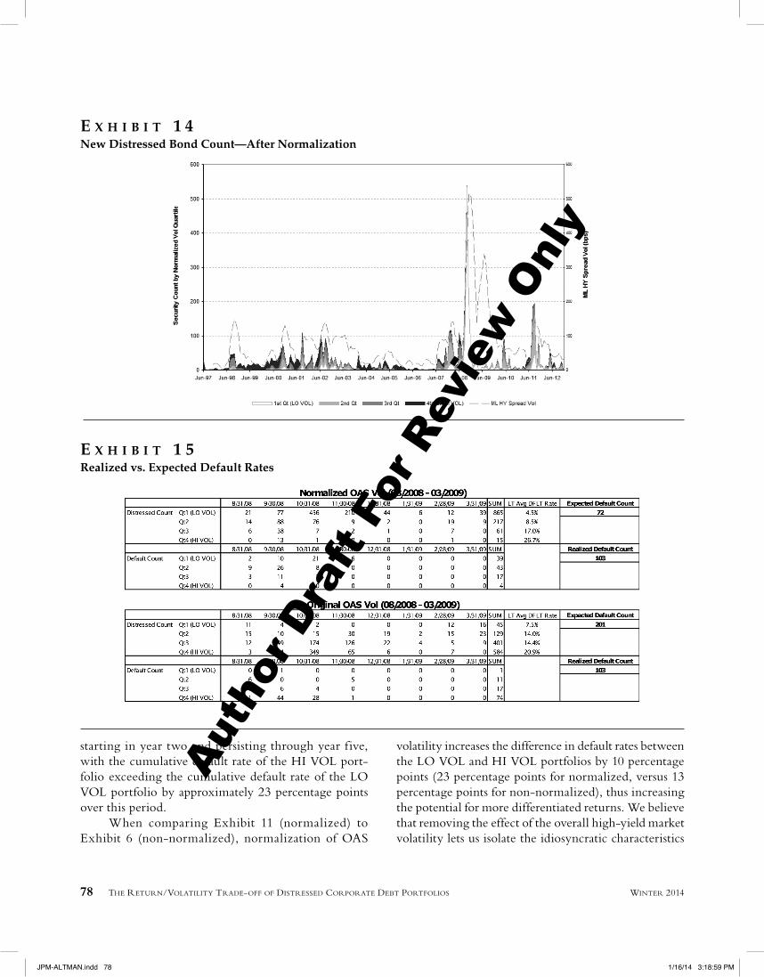
E X H I B I T 1 3New Distressed Bond Count—Before Normalization


Auth

or D

raft

For R

evie

w O

nly


starting in year two and persisting through year five, with the cumulative default rate of the HI VOL port-folio exceeding the cumulative default rate of the LO VOL portfolio by approximately 23 percentage points over this period.

When comparing Exhibit 11 (normalized) to Exhibit 6 (non-normalized), normalization of OAS

volatility increases the difference in default rates between the LO VOL and HI VOL portfolios by 10 percentage points (23 percentage points for normalized, versus 13 percentage points for non-normalized), thus increasing the potential for more differentiated returns. We believe that removing the effect of the overall high-yield market volatility lets us isolate the idiosyncratic characteristics

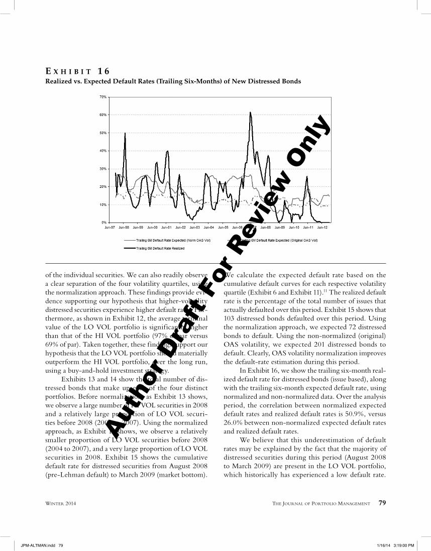
E X H I B I T 1 4New Distressed Bond Count—After Normalization

E X H I B I T 1 5Realized vs. Expected Default Rates


Auth

or D

raft

For R

evie

w O

nly


of the individual securities. We can also readily observe a clear separation of the four volatility quartiles, using the normalization approach. These findings provide evi-dence supporting our hypothesis that higher-volatility distressed securities experience higher default rates. Fur-thermore, as shown in Exhibit 12, the average terminal value of the LO VOL portfolio is significantly higher than that of the HI VOL portfolio (97% of par versus 69% of par). Taken together, these findings support our hypothesis that the LO VOL portfolio should materially outperform the HI VOL portfolio, over the long run, using a buy-and-hold investment strategy.

Exhibits 13 and 14 show the total number of dis-tressed bonds that make up each of the four distinct portfolios. Before normalization, as Exhibit 13 shows, we observe a large number of HI VOL securities in 2008 and a relatively large proportion of LO VOL securi-ties before 2008 (2003 to 2007). Using the normalized approach, as Exhibit 14 shows, we observe a relatively smaller proportion of LO VOL securities before 2008 (2004 to 2007), and a very large proportion of LO VOL securities in 2008. Exhibit 15 shows the cumulative default rate for distressed securities from August 2008 (pre-Lehman default) to March 2009 (market bottom).

We calculate the expected default rate based on the cumulative default curves for each respective volatility quartile (Exhibit 6 and Exhibit 11).11 The realized default rate is the percentage of the total number of issues that actually defaulted over this period. Exhibit 15 shows that 103 distressed bonds defaulted over this period. Using the normalization approach, we expected 72 distressed bonds to default. Using the non-normalized (original) OAS volatility, we expected 201 distressed bonds to default. Clearly, OAS volatility normalization improves the default-rate estimation during this period.

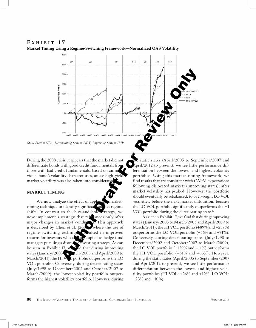
In Exhibit 16, we show the trailing six-month real-ized default rate for distressed bonds (issue based), along with the trailing six-month expected default rate, using normalized and non-normalized data. Over the analysis period, the correlation between normalized expected default rates and realized default rates is 50.9%, versus 26.0% between non-normalized expected default rates and realized default rates.

We believe that this underestimation of default rates may be explained by the fact that the majority of distressed securities during this period (August 2008 to March 2009) are present in the LO VOL portfolio, which historically has experienced a low default rate.

E X H I B I T 1 6Realized vs. Expected Default Rates (Trailing Six-Months) of New Distressed Bonds


Auth

or D

raft

For R

evie

w O

nly


During the 2008 crisis, it appears that the market did not differentiate bonds with good credit fundamentals from those with bad credit fundamentals, based on an indi-vidual bond’s volatility characteristics, unless high-yield market volatility was also taken into consideration.

MARKET TIMING

We now analyze the effect of applying a market-timing technique to identify significant market regime shifts. In contrast to the buy-and-hold strategy, we now implement a strategy that rebalances only after major changes in market conditions. This approach is described by Chen et al. [2008], where the use of regime-switching techniques resulted in improved returns for investors who allocate capital to hedge fund managers pursuing a distressed investing strategy. As can be seen in Exhibit 17, we find that during improving states ( January/2003 to March/2005 and April/2009 to March/2011), the HI VOL portfolio outperforms the LO VOL portfolio. Conversely, during deteriorating states ( July/1998 to December/2002 and October/2007 to March/2009), the lowest volatility portfolio outper-forms the highest volatility portfolio. However, during

the static states (April/2005 to September/2007 and April/2012 to present), we see little performance dif-ferentiation between the lowest- and highest-volatility portfolios. Using this market-timing framework, we find results that are consistent with CAPM expectations following dislocated markets (improving states), after market volatility has peaked. However, the portfolio should eventually be rebalanced, to overweight LO VOL securities, before the next market dislocation, because the LO VOL portfolio significantly outperforms the HI VOL portfolio during the deteriorating state.12

As seen in Exhibit 17, we find that during improving states ( January/2003 to March/2005 and April/2009 to March/2011), the HI VOL portfolio (+89% and +237%) outperforms the LO VOL portfolio (+56% and +71%). Conversely, during deteriorating states ( July/1998 to December/2002 and October/2007 to March/2009), the LO VOL portfolio (+129% and −11%) outperforms the HI VOL portfolio (−61% and −63%). However, during the static states (April/2005 to September/2007 and April/2012 to present), we see little performance differentiation between the lowest- and highest-vola-tility portfolios (HI VOL: +26% and +12%; LO VOL: +23% and +10%).

E X H I B I T 1 7Market Timing Using a Regime-Switching Framework—Normalized OAS Volatility

Static State = STA, Deteriorating State = DET, Improving State = IMP.


Auth

or D

raft

For R

evie

w O

nly


CONCLUSION

In summary, for a portfolio of distressed cor-porate high-yield bonds, we find that CAPM theory generally holds under two conditions: 1) using a time-independent theoretical framework, where no consider-ation is given to the overall volatility of the high-yield corporate debt market; and 2) using a time-dependent real-world framework, in which an investor possesses market-timing skills. However, CAPM expectations are not necessarily fulfilled in both time-independent and time-dependent space under a long-term buy-and-hold investment strategy, after adjusting for overall market volatility, because the LO VOL portfolio outperforms the HI VOL portfolio. We provide evidence that this

phenomenon is a result of the idiosyncratic characteris-tics of the distressed high-yield securities that comprise the LO VOL portfolio, which generate higher returns because they experience lower default rates and higher terminal values relative to the securities in the HI VOL portfolio. Because persistent market timing ability is a rare skill, investing in a buy-and-hold strategy com-prised of the lowest-volatility distressed securities may be a practical solution for the long-term investor.

A P P E N D I X A

ANNUALIZED RETURN DISTRIBUTION (ARD)—ORIGINAL OAS VOLATILITY

E X H I B I T A 1Distribution Functions of ARD Analysis

E X H I B I T A 2Characteristics of ARD Distribution Functions


Auth

or D

raft

For R

evie

w O

nly


A P P E N D I X B

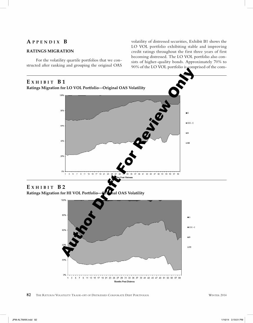
RATINGS MIGRATION

For the volatility quartile portfolios that we con-structed after ranking and grouping the original OAS

volatility of distressed securities, Exhibit B1 shows the LO VOL portfolio exhibiting stable and improving credit ratings throughout the first three years of first becoming distressed. The LO VOL portfolio also con-sists of higher-quality bonds. Approximately 70% to 90% of the LO VOL portfolio is comprised of the com-

E X H I B I T B 2Ratings Migration for HI VOL Portfolio—Original OAS Volatility

E X H I B I T B 1Ratings Migration for LO VOL Portfolio—Original OAS Volatility


Auth

or D

raft

For R

evie

w O

nly


bination of B and BB credits, with only 10% to 30% in CCC-C credits. This observation is remarkable in light of the fact that, after the second month in distress, the credit compositions of the two portfolios are less distinct

and quickly thereafter become highly differentiated, from a credit perspective. We also observe materially lower default rates for the LO VOL portfolio over the 60-month analysis period.

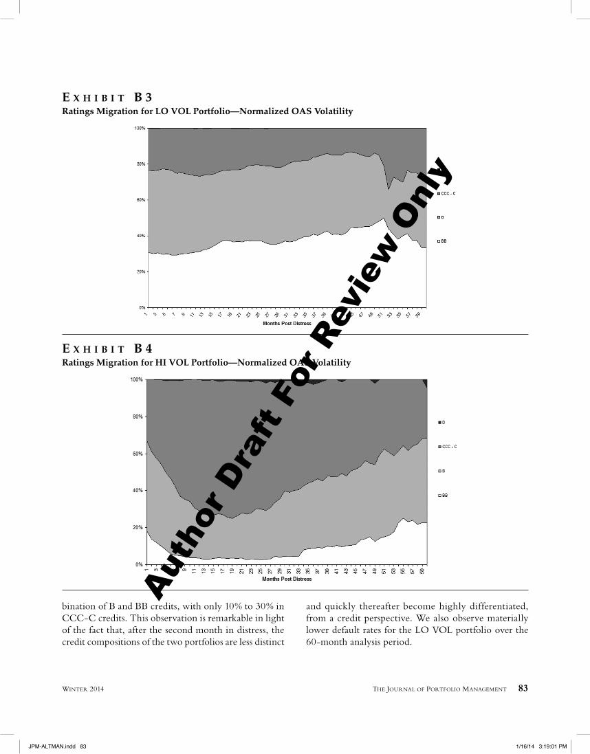
E X H I B I T B 3Ratings Migration for LO VOL Portfolio—Normalized OAS Volatility

E X H I B I T B 4Ratings Migration for HI VOL Portfolio—Normalized OAS Volatility


Auth

or D

raft

For R

evie

w O

nly


In contrast, Exhibit B2 shows that the HI VOL portfolio experiences an accelerated downward ratings migration during the first 12 months, and is generally composed of lesser-quality credits. Within the first year of becoming distressed, approximately 60% of the HI VOL portfolio migrates to CCC-C credits. Exhibits B3 and B4 show the credit rating migrations for the LO VOL and HI VOL portfolios that we constructed after ranking and grouping the normalized OAS volatility of distressed securities. By comparison, the LO VOL port-folio based on the original OAS volatility (Exhibit B1) and the LO VOL portfolio based on the normalized OAS volatility (Exhibit B3) share similar trends with regard to credit-rating migration. However, the LO VOL port-folio based on the normalized OAS volatility (Exhibit B3) contains more high-quality credits at the begin-ning of entering a state distress. Exhibit B4 shows faster deterioration in credit ratings for the HI VOL portfolio, based on normalized OAS volatility and a higher pro-portion of low-quality credits, such as CCC-C credits, over the analysis period.

ENDNOTES

1Harry Markowitz [1952] is recognized as laying the foundation for modern portfolio management theory. The CAPM theory was developed 12 years later in articles by William Sharpe [1964], John Lintner [1965], and Jan Mossin [1966].

2Edward I. Altman [1990] defined distressed securi-ties as: “…publicly held debt securities selling at sufficiently discounted prices so as to be yielding a minimum of 10% [1,000 bps] over comparable maturity US treasury bonds.” We use a slight modification of the definition, which uses the bond’s option-adjusted spread (OAS), in lieu of risk premium, which adjusts for the bond’s embedded call option in addition to incorporating the risk premium component. The latter is now the accepted market definition.

3High-yield market size (Source: Credit Suisse. Leverage Finance Strategy Monthly, January 2, 2013). Dis-tressed market size based on distressed ratio multiplied by size of high-yield market. (Source: BoA/ Merrill Lynch.)

4Private equity distressed/turnaround funds assets under management $180.23 billion (Thomson Reuters data-base). Hedge fund distressed funds assets under management $139.95 billion (Hedge Fund Research, Inc.: HFR Global Hedge Fund Industry Report – Year End 2012). All data as of December 31, 2012.

5The BofA Merrill Lynch US High-Yield Index (Bloomberg ticker H0A0) tracks the performance of U.S. dollar-denominated below-investment-grade corporate debt publicly issued in the U.S. domestic market. Qualifying secu-rities must have a below-investment-grade rating (based on an average of Moody’s, S&P, and Fitch). Source: Bank of America Merrill Lynch.

6There are three events that cause a default: bankruptcy, a missed interest payment not cured during the grace period, and a distressed exchange. In approximately 50% of cases, the default precedes the bankruptcy date when both occur, and in approximately 46% of cases, a distressed exchange is followed by a bankruptcy f iling. We calculate returns for defaulted securities, post default, as long as data is available. No value is assigned to any ultimate recovery arising from a bankruptcy restructuring or liquidation process. (See Altman and kuchne [2013]).

7A refinancing, tender offer, or any form of defeasance of the obligation is treated as a maturity.

8When we refer to the “first instance” of entering a state of distress, we measure and compare the spread volatility the second month after the OAS has exceeded 1,000 basis points. This is a result of the difference of means test between the Distressed Defaulted group and the Distressed Non-Defaulted group generating a significantly higher t-value (6.80). See Exhibit 1.

9For example, if we select starting and ending points of January 2003 and March 2005, the HI VOL portfolio (+89%) outperforms the LO VOL portfolio (+61%). If we select July 1997 and December 2002 as starting and ending points, we observe the opposite outcome, with the LO VOL portfolio (+13%) outperforming the HI VOL portfolio (-80%).

10The BofA Merrill Lynch US Distressed High Yield Index is a subset of The BofA Merrill Lynch U.S. High Yield Index that includes all securities with an option- adjusted spread greater than or equal to 1,000 basis points. The Bloomberg ticker symbol for the Distressed Index is H0DI. Source: Bank of America Merrill Lynch. The BofA ML Dis-tressed index rules remove high-yield securities when spreads fall below the threshold of 1,000 basis points. Therefore, if the security eventually matures when its OAS is less than 1,000 basis points, returns would be underestimated in the BofA Merrill Lynch H0DI index, relative to the methodology used in this article.

11Expected default rate = [(cumulative historical default rate of each volatility quartile) × (bond count of each vola-tility quartile)]/total bond count.

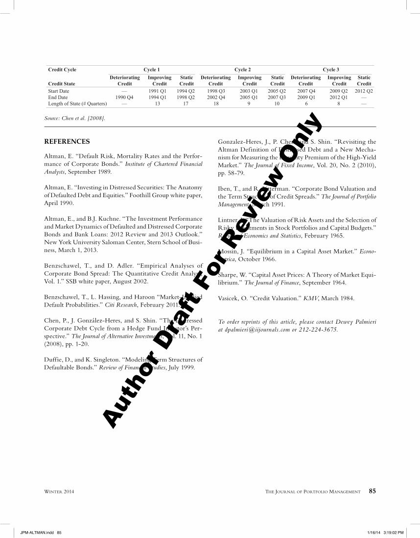
12The three distinct distressed cycles that have occurred since 1990 are defined thus:


Auth

or D

raft

For R

evie

w O

nly


Source: Chen et al. [2008].

REFERENCES

Altman, E. “Default Risk, Mortality Rates and the Perfor-mance of Corporate Bonds.” Institute of Chartered Financial Analysts, September 1989.

Altman, E. “Investing in Distressed Securities: The Anatomy of Defaulted Debt and Equities.” Foothill Group white paper, April 1990.

Altman, E., and B.J. Kuchne. “The Investment Performance and Market Dynamics of Defaulted and Distressed Corporate Bonds and Bank Loans: 2012 Review and 2013 Outlook.” New York University Saloman Center, Stern School of Busi-ness, March 1, 2013.

Benzschawel, T., and D. Adler. “Empirical Analyses of Corporate Bond Spread: The Quantitative Credit Analyst, Vol. 1.” SSB white paper, August 2002.

Benzschawel, T., L. Hassing, and Haroon “Market-Implied Default Probabilities.” Citi Research, February 2011.

Chen, P., J. González-Heres, and S. Shin. “The Distressed Corporate Debt Cycle from a Hedge Fund Investor’s Per-spective.” The Journal of Alternative Investments, Vol. 11, No. 1 (2008), pp. 1-20.

Duffie, D., and K. Singleton. “Modeling Term Structures of Defaultable Bonds.” Review of Financial Studies, July 1999.

Gonzalez-Heres, J., P. Chen, and S. Shin. “Revisiting the Altman Definition of Distressed Debt and a New Mecha-nism for Measuring the Liquidity Premium of the High-Yield Market.” The Journal of Fixed Income, Vol. 20, No. 2 (2010), pp. 58-79.

Iben, T., and R. Litterman. “Corporate Bond Valuation and the Term Structure of Credit Spreads.” The Journal of Portfolio Management, March 1991.

Lintner, J. “The Valuation of Risk Assets and the Selection of Risky Investments in Stock Portfolios and Capital Budgets.” Review of Economics and Statistics, February 1965.

Mossin, J. “Equilibrium in a Capital Asset Market.” Econo-metrica, October 1966.

Sharpe, W. “Capital Asset Prices: A Theory of Market Equi-librium.” The Journal of Finance, September 1964.

Vasicek, O. “Credit Valuation.” KMV, March 1984.

To order reprints of this article, please contact Dewey Palmieri at [email protected] or 212-224-3675.


Auth

or D

raft

For R

evie

w O

nly

the return/volatility trade-off of distressed …people.stern.nyu.edu/ealtman/the...

Documents