the resolving power of seismic amplitude data: an anisotropic inversion/migration...

GEOPHYSICS, VOL. 64, NO. 3 (MAY-JUNE 1999); P. 852–873, 16 FIGS., 5 TABLES.

The resolving power of seismic amplitude data: Ananisotropic inversion/migration approach

Maarten V. de Hoop∗, Carl Spencer‡, and Robert Burridge∗∗

ABSTRACT

A description of the theory and numerical implemen-tation of a 3-D linearized asymptotic anisotropic inver-sion method based on the generalized Radon transformis given. We discuss implementation aspects, including(1) the use of various coordinate systems, (2) regulariza-tion by both spectral and Bayesian statistical techniques,and (3) the effects of limited acquisition apertures oninversion. We give applications of the theory in whichwell-resolved parameter combinations are determinedfor particular experimental geometries and illustrate theinterdependence of parameter and spatial resolutions.Procedures for evaluating uncertainties in the parame-ter estimates that result from the inversion are derivedand demonstrated.

INTRODUCTION

The purpose of this paper is to investigate the use of thegeneralized Radon transform (GRT) for seismic inverse prob-lems involving anisotropic earth models. An understanding ofanisotropy is important for hydrocarbon exploration becauseshales, which make up 75% of the sedimentary cover of thehydrocarbon reserves, are almost invariably anisotropic. Theeffects of anisotropy on the kinematics of P-wave propagationand hence their effects on conventional seismic processing aresummarized in Larner and Tsvankin (1995). Ball (1995) pre-sented a real data example from a carbonate reservoir in theformer Zaire showing the effects of anisotropy on migration.

Anisotropy can also have a dramatic effect on the ampli-tude versus angle (AVA) response of a geological interface.As an example, in cases where shales and sands have simi-lar acoustic impedances, the introduction of anisotropy in theshale may bring about a change in sign of the reflection coef-ficient not present in the isotropic case. Similarly, it is possible

Published on Geophysics Online February 19, 1999. Manuscript received by the Editor December 30, 1996; revised manuscript received June 4, 1998.∗Colorado School of Mines, Center for Wave Phenomena, Golden, Colorado 80401-1887. E-mail: [email protected].‡Schlumberger Cambridge Research, High Cross, Madingley Road, Cambridge CB3 0EL, England, United Kingdom.∗∗Schlumberger-Doll Research, Old Quarry Road, Ridgefield, Connecticut 06877-4108.c© 1999 Society of Exploration Geophysicists. All rights reserved.

to encounter situations where amplitude anomalies that oth-erwise might be attributed to the presence of gas in isotropicmedia might also be caused by the presence of anisotropy inthe absence of gas. Our intention in this paper is to demon-strate a framework capable of answering the fundamentalquestions: What information about anisotropy do seismic am-plitudes reveal, and how do we use this information to imagerock properties?

Over the past decade, substantial progress has been madetowards solving the problem of inverting seismic data to yieldmodels of the physical properties of the earth. Several differ-ent techniques have been suggested by various scientists basedon what, at first sight, seem like very different approximationsof the inverse problem, but which turn out in practice to bearmany similarities. The different techniques can be classified ac-cording to (1) the method of carrying out the forward modeling(for example, full-waveform, Kirchhoff, ray-Born, etc.), (2) themethod of inverting the forward relation (for example, nonlin-ear local optimization possibly preceded by preconditioning,or the direct GRT), (3) the parameterization of the subsurface(scalar, isotropic elastic, anisotropic elastic, and poro-elasticrepresent increasingly sophisticated medium descriptions).Also, the choice of a forward modeling approach usually im-plies a particular discretization of the scattering domain, i.e.,the subsurface. It is the second classification (2) that is mostfundamental to a discussion of practical inversion methods.

Perhaps the most obvious way of solving the seismic inverseproblem is to search parameter space by techniques such asthe conjugate gradient minimization of some measure of themisfit between observed and simulated seismograms. Such anapproach was developed for the acoustic case by Bambergeret al. (1982) and was subsequently modified and extended bynumerous authors (Tarantola, 1984, 1986; Gauthier et al., 1986;Ikelle et al., 1986; Beydoun and Mendez, 1989; Mora, 1989;Singh et al., 1989; Snieder et al., 1989; Cao et al., 1990; Eatonand Stewart, 1994; Debski and Tarantola, 1995). Two essen-tial features of all these search methods are the use of iter-ative solutions to the (nonlinear) optimization problem and

852

Downloaded 09 Apr 2009 to 128.210.4.214. Redistribution subject to SEG license or copyright; see Terms of Use at http://segdl.org/

Anisotropic Inversion/Migration 853

regularization by inclusion of a priori information. Cheng andCohen’s (1984) and Tarantola’s (1984) observation that inver-sion can be expressed in terms of more conventional seismicprocessing methods is a recurring motif in the literature that ap-plies to almost all common approaches to the inverse problem(Bleistein and Cohen, 1979; Clayton and Stolt, 1981; Mora,1989; Claerbout, 1992).

A second suite of inverse methods originated in the field ofultrasonics (Norton and Linzer, 1981) and is based on approxi-mations to the forward and inverse formulations that permit di-rect, closed-form expressions for the inverse problem solution(Clayton and Stolt, 1981; Devaney, 1984; Beylkin, 1985; Milleret al., 1987; Bleistein, 1987; de Hoop et al., 1994; Burridge et al.,1998). The majority of these methods use the Born approxi-mation to model scattering at the target together with asymp-totic approximations such as WKBJ or asymptotic ray theoryfor propagation to and from the scatterer. Solutions are thenobtained by mappings, such as the GRT, which require fur-ther high-frequency approximations. Since the starting pointfor both the direct and search-based inversion techniques isa weak formulation of the inverse problem, the mechanicsof both methods can turn out to be similar (Esmersoy andOristaglio, 1988; Jin et al., 1992). It is also possible to use oper-ators obtained using direct linearized methods asymptoticallyas preconditioners for search-based nonlinear optimization (deHoop and de Hoop, 1997).

In this paper, we will be exclusively concerned with themultiparameter elastic inverse problem. Several approaches tomultiparameter inversion have been proposed in the isotropiccase. Berkhout and Wapenaar (1990) suggested that wave-field decomposition be applied at an early stage in process-ing the data so that P and S pseudoscalar wavefields or po-tentials can be inverted separately. Bleistein (1987) modifiedthe generalized Radon transform method of Beylkin (1985)and Miller et al. (1987) to the three-parameter elastic case byformulating the problem as Kirchhoff scattering from inter-faces rather than Born scattering from volumes. The inversionprocess involved two parallel integrations (weighted diffrac-tion stacks) that allow both reflection coefficient as a functionof angle and the angle of specular reflection to be recoveredat each image point. Beylkin and Burridge (1990) proposeda multiparameter scheme based on the Born approximationinstead. A GRT inversion was designed to construct an inter-mediate vector quantity from which elastic parameters couldbe recovered. This method avoided the need for dividing twoimage sections to provide angle information, as required bythe method of Bleistein (1987). Among the optimization ap-proaches, Tarantola (1986), Beydoun and Mendez (1989), andJin et al. (1992) have considered the isotropic multiparam-eter problem. Parameter estimates are obtained by a back-propagation of the residual wavefield followed by convolutionwith an approximate inverse Hessian arising from the locallinearization of the forward contrast-source formulation.

The introduction of anisotropy into elastic seismic inversionincreases the number of possible parameters needed to specifythe physical properties of a point within the earth to 22. Thisis far more than can be recovered in practice and, therefore,attention must be given to reducing the size of the problem.One possible approach is to understand the scattering processwell enough beforehand to be able to provide a limited num-ber of combinations of parameters that describe the process

effectively. Banik (1987) and Tsvankin and Thomsen (1995)have done so for the case of weak scattering in VTI (trans-versely isotropic with vertical axis of symmetry) media andfind that near-normal incidence P-wave scattering behavior iscontrolled by vertical impedance contrast and the parameter δ(Thomsen, 1986). This analysis has been extended to the caseof orthorhombic media with a symmetry plane aligned witha planar scattering interface (Ruger, 1996). In more generalcases and with arbitrary recording geometries, it may be lessobvious which parameter combinations to use. The alternativeapproach, and the one adopted in this paper, is to use linear in-verse theory to evaluate the “best resolved” parameter. We usethe phrase “best resolved parameter” to refer to the combina-tion of elastic moduli at an image point that is least dependenton other combinations of moduli at the same image point. Inmultiparameter inverse problems, the resolving power of an ex-periment is made up of two parts. Spatial resolution quantifiesthe blurring of the image in space, whereas the parameter res-olution quantifies the linear interdependence of elastic moduliand density. Both effects are described by a resolution operatorthat will be discussed in this paper. A second feature of usinglinear inverse theory is that it is possible to calculate estimatesof parameter uncertainty by mapping noise in the data, whichmay be described as a data covariance matrix, into errors inestimates of moduli.

Both the GRT and optimization approaches to the inversionof seismic data for anisotropic parameters have been attempted(de Hoop et al., 1994; Eaton and Stewart, 1994; Burridge et al.,1998). All these authors used a Born formulation for the for-ward problem and all account for ill-posedness in the parame-ter part of the problem by solving a reduced linear system via asingular value decomposition. A significant difference betweenthe isotropic and anisotropic inversion cases is that most di-rect isotropic multiparameter inverse methods yield algorithmsthat can be described as migration followed by inversion (i.e.,energy is positioned before an amplitude versus scattering an-gle or offset relationship is inverted). Such an ordering is notappropriate for the anisotropic case because the scattering re-sponse of an elastic modulus such as C33 no longer depends onscattering angle alone. It is a function of both scattering angleand interface normal direction (or more correctly the gradientin total traveltime). Burridge et al. (1998) discuss this prob-lem in detail and formulate extensions to the GRT algorithmof Miller et al. (1987) for anisotropic media. The algorithm,which will be discussed further in the following sections, canbe separated into an AVA inversion for each migration dip,followed by migration, the integration over dips—hence thetitle of this paper.

In the remainder of this paper, we develop the anisotropicGRT inversion theory, paying special attention to the calcula-tion of the various Jacobians involved, and address the issuesof regularization and acquisition aperture compensation. Wethen provide several synthetic examples illustrating the essen-tial features of the method and draw general conclusions.

SOURCE-RECEIVER RAY GEOMETRY

Our intention in the following sections is to present a mathe-matical description of our inversion procedure, emphasizing as-pects such as recording geometries, ill-posedness, and aperturelimitation that arise in practical applications. The development


854 de Hoop et al.

here is for the 3-D case, and we will make use of asymptotictheories applicable to high-frequency wave propagation andinversion for the most singular constituents of the medium.More complete descriptions of the ray-theory Green’s functioncalculations can be found in Kendall et al. (1992) and of theinversion method in de Hoop et al. (1994) and Burridge et al.(1998). In Tables 1 and 2, a glossary of symbols is provided.

We begin by giving ray-theoretical expressions for the propa-gation of phase and amplitude in anisotropic media with elasticmoduli ci jk` (Voigt notation: CI J , I , J= 1, . . . , 6) and density ρ(Shearer and Chapman, 1989; Kendall et al., 1992). Let τ bethe arrival time and ξ the associated polarization vector. Weuse x to denote a point inRR3, subscripts denote components ofvectors and tensors, and ∂ j denotes partial differentiation withrespect to the j th component of x. The polarization vectors areassumed to be normalized so that ξi ξi = 1. Define the slownessvector γ by

γ(x) = ∇xτ (x, x′) (1)

along the ray originating at x′. Then γ and ξ satisfy the “eigen-value” equation

(ρδik − ci jk`γ`γ j )ξk = 0 (at all x). (2)

Equation (2) constrains γ to lie on the sextic surface, A(x),given by

det(ρδik − ci jk`γ`γ j ) = 0. (3)

By virtue of equation (1), equation (3) may be interpreted asa nonlinear partial differential equation, the eikonal equation,for τ . The surface A(x) consists of three sheets, each of which

Table 1. Glossary of symbols: ray geometry.

In or nearSymbol equation number Meaning

s (11) Source positionx, y (11), (26) Scattering point,

image pointr (11) Receiver positionτ (1) One-way traveltimeA (5) Scalar amplitudeγ (1) Local slowness vectorV (7) Local phase velocityα (8) Local phase directionA (3) Local slowness surfacev (6) Local group velocityχ (9) Angle between group

and phase velocities6 (16) Wave front surfaceM (10) Amplitude Jacobianξ (2) Local polarization vectorH (4) Hamiltonianσ (10) KMAH indexH (10) Hilbert transformT (15) Two-way traveltimeΓ (16) Gradient of two-way timeΘ (35) Migration wave vectorν (19) Migration dip, isochron

normalθ (20) Scattering angleψ (20) Azimuth

is a closed surface surrounding the origin. An individual sheetis described by equation (2), leading to

H(x,γ) = 12 (ρ − ξi ci jk`γ`γ j ξk) = 0, (4)

where γ varies continuously and ξ is the eigenvector belongingto γ. The three sheets are commonly thought of as correspond-ing to one quasi-compressional and two quasi-shear waves. Hdenotes a Hamiltonian that generates the ray-tracing equations(Kendall et al., 1992).

The scalar amplitudes A must satisfy the transport equation

∂ j(ci jk`ξi ξk(A)2∂`τ

) = 0 (5)

for each mode of propagation.For each mode the characteristic or group velocity v is nor-

mal to A(x) at γ and satisfies

v · γ = 1; v = ∇γHγ · ∇γH

∣∣∣∣H=0

. (6)

The normal or phase speed is given by

V = 1|γ| . (7)

Table 2. Glossary of symbols: GRT.

In or nearSymbol equation number Meaning

∂S (17) Surface of source locations∂R (17) Surface of receiver locationsβ, β (45) Normals to ∂S, ∂RNs (58) Number of sourcesNr (58) Number of receiversN (58) Number of measurementsN (17) Quasi midpointΩ (17) Quasi half offsetu (22) Scattered displacement filedσu (50) Data covarianceD (17) Scattering domain, support

of medium perturbationc(1) (22) Perturbation in density

and stiffnessσc (50) Medium covarianceP (52) Medium parameter projectionδ(1) (52) Perturbation in generic

medium parametersw (22) Contrast-source radiation

patternsI (23) Weight in the forward GRT3,3a (25), (30) Normal matrix of

radiation patternsJ ,Ja (27) Weight in the GRT inversionh, ha (28), (33) ObliquityEν (56) Support in dipEθ (25) Support in scattering

angle for fixed dipEψ (25) Support in azimuth for fixed

dip and scattering angleEα (51) Support in phase directions

for fixed dipC (57) Aperture normalization factorRC (56) Resolution kernel



The unit phase direction follows as

α = Vγ. (8)

From equation (6), it then follows that

V = |v| cosχ, (9)

where χ is the angle between v and γ.Ray-theoretical displacement amplitudes, satisfying the

transport equation and originating from a point force source(a vibrator) at x′, can be written in terms of a Jacobian Mdescribing the geometrical spreading along a ray:

A = 14π [ρ(x)ρ(x′)M]1/2

with M =|v(x′)|V(x)

∣∣∣∣ ∂x∂q1∧ ∂x∂q2

∣∣∣∣x∣∣∣∣ ∂γ∂q1

∧ ∂γ

∂q2

∣∣∣∣x′

. (10)

Here, (q1,q2) parametrize the rays originating from the sourceand can be chosen to lie on the unit sphere (S2), centered at x′.In the presence of caustics, in the Green’s tensor, the scalar am-plitude will carry a phase shift π/2 to the power of the KMAHindex σ (x; x′;γ(x′)) inducing the contribution from a Hilberttransform H. Away from any intrinsic caustic associated withthe anisotropy of the medium, the index characterizes the localcurvature of the slowness surface sheet, where the index is 0 ifthe surface is convex, 1 if the surface is saddle shaped, and 2 ifthe surface is concave.

Source and receiver rays

To describe rays from a point in the subsurface to sourcesand receivers, we introduce a notation in which ˜ refers to anyquantity ` associated with the source, and ˆ refers to the samequantity associated with the receiver. Thus, the geometricalamplitudes to a source at s and a receiver at r will be written as

A(x) = A(x, s), A(x) = A(r, x). (11)

According to equation (1), the slowness vectors at x are givenby

γ(x) = ∇xτ (x, s), γ(x) = ∇xτ (r, x), (12)

the associated phase directions are given by

α = γ

|γ| , α = γ

|γ| , (13)

and the directional phase speeds [cf. equation (7)] are given by

V = 1|γ| , V = 1

|γ| . (14)

We also define the two-way traveltime T and its gradient,

T(r, x, s) ≡ τ (x, s)+ τ (r, x),(15)

Γ(r, x, s) ≡ ∇xT(r, x, s).

From equation (12), we see that

Γ(r, x, s) = γ(x)+ γ(x). (16)

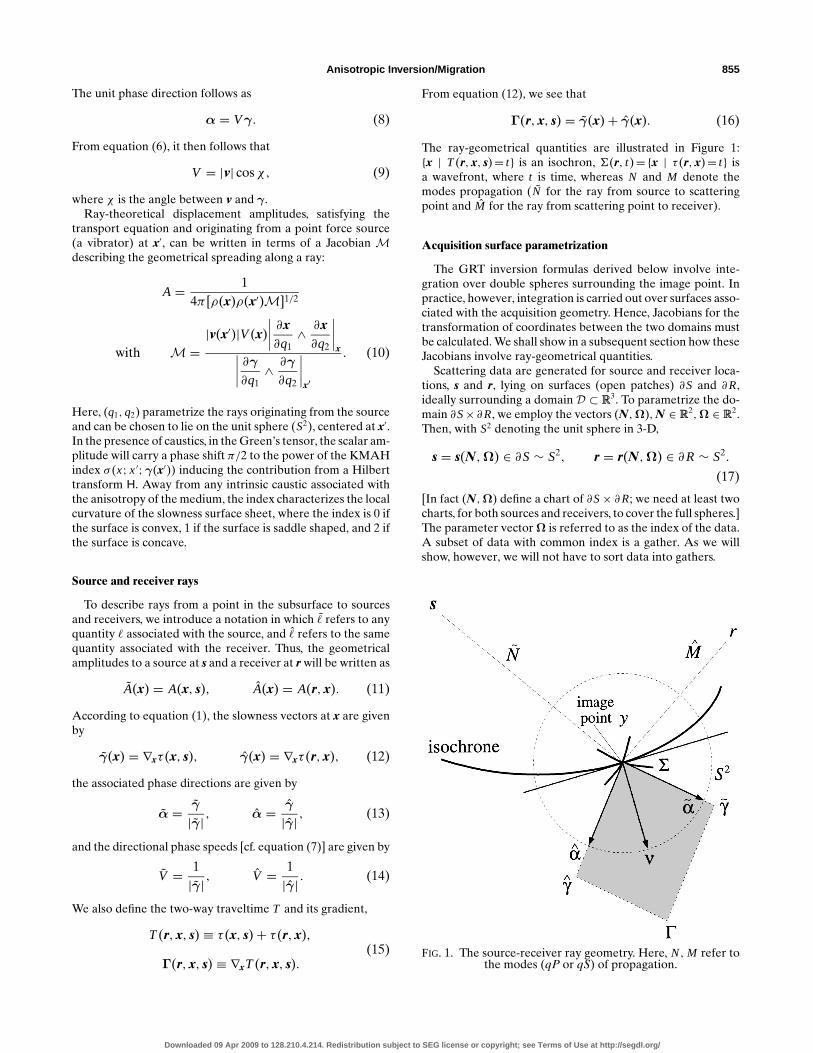
The ray-geometrical quantities are illustrated in Figure 1:x | T(r, x, s)= t is an isochron, 6(r, t)=x | τ (r, x)= t isa wavefront, where t is time, whereas N and M denote themodes propagation (N for the ray from source to scatteringpoint and M for the ray from scattering point to receiver).

Acquisition surface parametrization

The GRT inversion formulas derived below involve inte-gration over double spheres surrounding the image point. Inpractice, however, integration is carried out over surfaces asso-ciated with the acquisition geometry. Hence, Jacobians for thetransformation of coordinates between the two domains mustbe calculated. We shall show in a subsequent section how theseJacobians involve ray-geometrical quantities.

Scattering data are generated for source and receiver loca-tions, s and r, lying on surfaces (open patches) ∂S and ∂R,ideally surrounding a domain D ⊂ RR3. To parametrize the do-main ∂S× ∂R, we employ the vectors (N,Ω),N ∈ RR2,Ω ∈ RR2.Then, with S2 denoting the unit sphere in 3-D,

s = s(N,Ω) ∈ ∂S∼ S2, r = r(N,Ω) ∈ ∂R∼ S2.

(17)

[In fact (N,Ω) define a chart of ∂S× ∂R; we need at least twocharts, for both sources and receivers, to cover the full spheres.]The parameter vector Ω is referred to as the index of the data.A subset of data with common index is a gather. As we willshow, however, we will not have to sort data into gathers.

FIG. 1. The source-receiver ray geometry. Here, N,M refer tothe modes (qP or qS) of propagation.


856 de Hoop et al.

As an example, let s and r lie in a plane. Then indexing inhalf-offset with Ω= (1/2)(r − s) fixed (common) yields

s = N −Ω, r = N +Ω, (18)

where N = (1/2)(s+ r) denotes the midpoint. On the otherhand, common receiver gathers induce s=N, r=Ω, whereascommon source gathers correspond to s=Ω, r=N. In the idealsituation, two charts (N) define a domain ∂N ∼ S2 (throughstereographic projection) for any Ω fixed (common). All theseindexings are independent of the elastic properties of the sub-surface.

However, for the purpose of GRT inversion, the natural in-dexing will be image-point dependent. We will discuss the in-dexing in scattering-angle/azimuth. Let ν denote the migrationdip at image point x ∈ D, i.e.,

ν(r, x, s) = |Γ|−1 Γ; (19)

the scattering angle θ and azimuth ψ are then defined through

cos θ = α · α, ψ = third Euler angle aroundν.

(20)

Note that ν ∈ S2 and (θ, ψ) ∈ S2. Then ν replaces the role ofN and (θ, ψ) replaces the role of Ω. Our key constraint is thatN must map ν uniquely on the sphere S2 for any fixed Ω.

The various transformations on S2× S2 are summarized inTable 3.

GENERALIZED RADON TRANSFORMATIONS

In the remainder of the paper, we exclude the occurrenceof rays originating in the scattering domain, traveling in thebackground medium, and grazing at ∂Ror ∂S. Also, we assumethat ∂S and ∂R cannot be connected by a single ray travelingthrough the scattering domain (then the migration dip wouldnot be defined). In principle, multipathing in the backgroundcan be accounted for, in which case the integrations over dipand scattering angles are inseparable (D.-J. Smit, personal com-munication, 1996).

First, we will write the direct scattering problem in the formof a GRT. Second, for y in the neighborhood of x, usingBeylkin’s (1985) analysis of this transform,∫

S2[1+O(|x − y|)]δ′′(ν · (y− x)+O(|x − y|2)) dν

= −8π2δ(y− x)+ smoother terms, (21)

where O(|x − y|) and O(|x − y|2) as |x − y| → 0 may dependon ν, we will derive the GRT inversion.

The forward transform

The scattered field u due to a contrast in medium parametersc(1) with bounded support D ⊂ RR3, in the ray-Born approxi-

Table 3. Coordinate transformations in the GRT.

(α, α)x → (ν, (θ, ψ))x (ν, (θ, ψ))x → (s, r)(α, α)x → (s, r) (s, r)→ (N,Ω)

mation, can be written in the form of a GRT:

u(t, r, s) ' −∫Dδ′′(t − T(r, x, s))

× (w(r, x, s))T c(1)(x)I(r, x, s) dx, (22)

where

I(r, x, s) = ρ(x)A(x)A(x). (23)

Here, ρ is the density of the background medium, A is the(point-source) amplitude along the ray connected to the sourcelocation, A is the (point-source) amplitude along the ray con-nected to the receiver location, T(r, x, s) is the traveltime inthe background medium along the ray connecting the sourcewith the receiver via the scattering point x, and w representsthe radiation patterns of point contrast sources at the scatteringpoint in accordance with the stiffness-density parametrizationc. The radiation patterns are symmetrized dyadic products ofthe four polarization and slowness vectors at the scatteringpoint, associated with the rays to the source and to the re-ceiver [Burridge et al., 1998, equation (3.30)]. In our notation,we have suppressed the occurrence of the Hilbert transforms.We have arranged the tensors w and c in arrays. The integralin equation (22) is taken over isochrons. We freely identify

T(x,N,Ω) = T(r, x, s), w(x,N,Ω) = w(r, x, s),

or

T(x, α, α) = T(r, x, s), w(x, α, α) = w(r, x, s),

through the respective coordinate transformations of Table 3.

The inverse transform over phase directions at the image point

The structure of the dual GRT transform (Beylkin, 1985),associated with equation (22), follows as

〈c(1)〉(x,Ω) ' 18π2

∫∂NJ (r, x, s)[3x(ν(r, x, s))]−1

×wu(T(r, x, s), r, s)∂(α, α)∂(N,Ω)

∣∣∣∣x

dN, (24)

where ν is the unit vector in the direction of ∇xT [equa-tion (19)], α is the normalized slowness vector associated withthe ray connected to the receiver, α is the normalized slownessvector associated with the ray connected to the source, and

3.(ν) =∫

Eθ (ν)

∫Eψ (ν,θ)

(wwT )∂(α, α)∂(ν, θ, ψ)

∣∣∣∣.

dψ dθ (25)

unravels the radiation patterns at the image point (E denotessupport). The hypersurface

(Ω, t) ∈ ∂Ä× RR≥0 | t = T(r(N,Ω), x, s(N,Ω))is the so-called diffraction surface, and equation (24) describesnothing other than the diffraction stack with weights J , whichare determined below.



The inverse GRT (i.e. J ) follows from composing the for-ward with the dual transforms. We then obtain the condition,at stationarity,[− 1

8π2

∫∂Nδ′′(T(r, y, s)− T(r, x, s))J (r, y, s)I(r, x, s)

× ∂(ν, θ, ψ)∂(N,Ω)

∣∣∣∣y

dN]

dΩ = δ(y− x) dθ dψ

+ smoother terms. (26)

Using the homogeneity of δ′′ and the plane-wave expansion ofthe Dirac distribution equation (21), we find that

J (r, x, s) = h(x,ν(r, x, s))I(r, x, s)

, (27)

with

h = |Γ|3. (28)

In the presence of caustics, the data u in equation (24) need bereplaced by u+ i Hu and the real part of the integral has to betaken (details can be found in de Hoop and Brandsberg-Dahl,1998). Note that h acts as a natural taper on the measurementsfor large scattering angles. The AVA inversion amounts now tointegrating 〈c(1)〉(x,Ω) over Ω to yield the elastic parameters,but note that the inverse [3.(ν)]−1 is essentially nested in theintegration over N or ν (the migration).

Carrying out the AVA inversion simultaneously with the mi-gration allows the integration in equation (24) followed by theintegration in equation (25) both to be directly carried out over(α, α) with volume form dαdα; note that s and r then followfrom the intersection of the rays with ∂Sand ∂R, respectively.

The inverse transform over acquisition parametersat the surface

It is possible to reformulate the inverse problem using thecoordinates naturally arising in the acquisition geometry, whichis the conventional approach to GRT inversion. We will distin-guish this representation of the GRT from the previous one byusing super- and subscripts a. Then, the structure of the dualGRT transform follows as

〈c(1)〉(x,Ω) ' 18π2

∫∂NJa(r, x, s)

[3a

x(ν(r, x, s))]−1

×wu(T(r, x, s), r, s) dN, (29)

with (ν at x maps onto N)

3a. (ν) =

∫EΩ(N)

(wwT )∣∣∣∣.

dΩ (30)

((θ, ψ) at x for ν fixed map onto Ω). Matching the condition[the counterpart of equation (26)], at stationarity,[− 1

8π2

∫∂Nδ′′(T(r, y, s)− T(r, x, s))Ja(r, y, s)

× I(r, x, s) dN]

dΩ = δ(y− x) dΩ+ smoother terms,

(31)

using plane-wave expansion equation (21) as before, we findthat

Ja(r, x, s) = ha(x,ν(r, x, s))I(r, x, s)

, (32)

where now

ha = |Γ|3(∂(ν)∂(N)

)Ω. (33)

If we allow (N,Ω) to be x dependent, we can set N =ν andΩ= (θ, ψ). Then, equation (33) reduces to equation (28). Thiscorresponds precisely to indexing the measurements in com-mon scattering-angle/azimuth gathers (which varies with imagepoint).

The integration over ν or N should produce the same image(singular support of the perturbation c(1)) for each pair (θ, ψ) orΩ. This redundancy, comparing those images, can be used to im-prove the background velocity model by the method of differ-ential semblance (or coherency) optimization (Carazzone andSymes, 1991; Symes and Kern, 1994), residual curvature anal-ysis (Liu, 1995), or by maximizing a similarity index (Chavent& Jacewitz, 1995). Such an improvement captures part of thetruly nonlinear aspects of the seismic inverse problem.

Fourier analysis

To link the GRT approach to inversion/migration withFourier “ f -k” (ω= 2π f ) migration, we use the one-sidedFourier representation of the Dirac distribution to rewrite con-dition (26):

18π3

[ ∫∂N

∫RR≥0

exp[iω(T(r, y, s)− T(r, x, s))]J (r, y, s)

× I(r, x, s)∂(ν, θ, ψ)∂(N,Ω)

∣∣∣∣yω2 dω dN

]dΩ = δ(y− x) dθ dψ

+ smoother terms. (34)

We introduce the wave vector

Θ = ωΓ ∈ RR3 at x, (35)

since, in the high-frequency approximation, the phase in equa-tion (34) can be approximated according to

ω(T(r, y, s)− T(r, x, s)) ' Θ · (y− x) (36)

up to leading order. We carry out the mapping

(ω,ν)→ Θ;the inverse mapping

ω(Θ) = Θ · Γ|Γ|2

also appears in Stolt’s formulation (Stolt, 1978). Then equa-tion (34) can be written in the form


858 de Hoop et al.

18π3

∫RR3

exp[i Θ · (y− x)]J (r, y, s)I(r, x, s)

×ω2 ∂(ω,ν)∂(Θ)

∣∣∣∣y

dΘ

= δ(y− x)+ smoother terms. (37)

It now follows from the Fourier representation of the Diracdistribution that

J (r, x, s) = 1I(r, x, s)

1ω2

∂(Θ)∂(ω,ν)

∣∣∣∣x. (38)

Note, however, that

1ω2

∂(Θ)∂(ω,ν)

= ∣∣det(Γ ∂ν1Γ ∂ν2Γ

)∣∣ = h (39)

yields the previous result [equation (28)]. Condition (31) re-sults, in a likewise manner, in

Ja(r, x, s) = 1I(r, x, s)

1ω2

∂(Θ)∂(ω,N)

∣∣∣∣x. (40)

Here,

1ω2

∂(Θ)∂(ω,N)

= ∣∣det(Γ ∂N1Γ ∂N2Γ

)∣∣ = h

(∂(ν)∂(N)

)Ω,

(41)

which is Beylkin’s original determinant (Beylkin, 1985). For thecomputation of this determinant, note that in general, regularsampling in ν will cause irregular sampling in N and vice versa.

JACOBIANS

Transformation from phase directions tosource-receiver coordinates

We have

∂(α, α)∂(N,Ω)

∣∣∣∣y= ∂(α, α)

∂(s, r)

∣∣∣∣y

∂(s, r)∂(N,Ω)

. (42)

The Jacobian, with factorization (α does not depend on r andα does not depend on s)

∂(α, α)∂(s, r)

∣∣∣∣y= ∂(α)∂(s)

∣∣∣∣y

∂(α)∂(r)

∣∣∣∣y, (43)

is directly related to dynamic ray theory. In general, the factorscan be expressed in terms of the dynamic ray amplitudes be-cause, like the amplitudes, they follow from a variation of theanisotropic ray tracing equations [see equation (10)]. For thesource side,

∂(s6)∂(α)

∣∣∣∣y= 1

16π2ρ(s)ρ(y)V(s)(V(y))3(A(y))2(44)

as long as ∂S in the neighborhood of s coincides with the wavefront 6(y, τ (s, y)) originating at y. If this is not the case, we

have to correct for the ratio of the area on ∂S to the areaon the wave front 6(y, τ (s, y)) at s onto which it is mapped byprojection along the rays. This arises from the fact that ∂Sis notnecessarily tangent to 6(y, τ (s, y)) at s. It amounts to dividingthe previous Jacobian by the Jacobian

∂(s6)∂(s)

= (α(s) · β(s)), (45)

where s6 denotes the coordinates on 6(y, τ (s, y)) intersecting∂S at s, and β(s) = normal to ∂S at source. Note that α(s) isthe normal to the wavefront at s. Similar expressions hold forthe receiver side.

Transformation from phase directions to dip, scatteringangle, and azimuth

Under the transformation from phase directions to dip, scat-tering angle, and azimuth, the volume form on S2× S2 [cf.equation (25)] transforms according to

∂(α, α)∂(ν, θ, ψ)

= sin θ1+ (|γ‖γ|/|Γ|2)(tan χ − tan χ) sin θ

,

(46)where

Γ = ∇xT, cos χ = n‖ · α, and cos χ = n‖ · α(47)

(see Appendix A). Here, n‖ and n‖ denote the normals to theslowness surface at the scattering point projected in the az-imuth plane ψ .

Transformation from dip to midpoint at fixed half-offset

With equation (41), the Jacobian associated with the map-ping ν → N can be expressed in terms of

det(Γ ∂N1Γ ∂N2Γ

) = Γ · (∂N1Γ ∧ ∂N2Γ), (48)

in which

∂N1,2Γ = (∂N1,2s) · ∇sγ +

(∂N1,2r

) · ∇rγ. (49)

In principle, ∇sγ and ∇rγ can be computed by perturbing theHamilton system for ray tracing. For a homogeneous, isotropicmedium, the evaluation of this Jacobian is reviewed in Ap-pendix B.

REGULARIZATION

The inversion of the 3 matrix in general requires a regular-ization because some of its singular values may become verysmall or even vanish (Campbell and Meyer, 1979). We considertwo approaches in our analysis. The first one is based on a sin-gular value decomposition in the inversion process and can beinterpreted in terms of Bayesian statistics; the second one isbased on a straightforward parameter reduction.

In the Bayesian approach we introduce an a priori probabil-ity distribution of allowable models with covariance matrix σc.The prior model estimate is denoted as c(1)

prior. Also, we introduce



a likelihood distribution in the space of measured displace-ments (scattered field) u with covariance σu(θ, ψ), constrainedto be diagonal. Assuming Gaussian statistics, equation (25) ismodified to

3.(ν) =∫

Eθ (ν)

∫Eψ (ν,θ)

(wσ−1

u wT)

(50)

× ∂(α, α)∂(ν, θ, ψ)

∣∣∣∣.

dψ dθ + σ−1c .

This matrix has the interpretation of reciprocal of the a poste-riori multiparameter covariance matrix σ ′c for dip ν. Note thatσ−1

c controls the shift of singular values. The square roots ofthe elements of the diagonal of 3.(ν) are the standard devia-tions of the solution to the AVA—amplitude versus scatteringangles—inverse problem at dip ν. Let the generalized inverseof the matrix 3.(ν) be denoted as 〈[3.(ν)]−1〉, then the inver-sion formula equation (24) is subject to the modification

[3.(ν)]−1wu→ 〈[3.(ν)]−1〉[

wσ−1u u

+ 1|Eα(ν)|σ

−1c c(1)

prior

], (51)

|Eα(ν)| ≡∫

Eθ (ν)

∫Eψ(ν,θ)

∂(α, α)∂(ν, θ, ψ)

∣∣∣∣.

dψ dθ.

In the absence of prior information, c(1)prior= 0, and the param-

eter resolution matrix for dip ν is given by

〈[3.(ν)]−1〉3.(ν),

whereas the sensitivity matrix follows from the mapping of datacovariances to a posteriori co-variance matrix σ ′c for dip ν,

(σ ′c)(ν) =∫

Eθ (ν)

∫Eψ (ν,θ)

〈[3.(ν)]−1〉w(.)σu(θ, ψ)(w(.))T

×〈[3.(ν)]−1〉T ∂(α, α)∂(ν, θ, ψ)

∣∣∣∣.

dψ dθ.

Naturally, σu has to be estimated directly from the data in thecommon dip domain.

Parameter reduction, on the other hand, independent of sta-tistical considerations, can be represented by a projection ma-trix P. Let

c(1)(x) = PTδ(1)(x) (52)

such that δ is contained in a µ-dimensional parameter space,µ ≤ 22. The technique of reparametrization provides anothertool to turn the inverse problem into a well-posed one. In allthe equations, we simply have to replace c(1) by δ(1) and w byPw. Note that 3 reduces to the µ×µ matrix

3.(ν) =∫

Eθ (ν)

∫Eψ (ν,θ)

Pw (Pw)T ∂(α, α)∂(ν, θ, ψ)

∣∣∣∣.

dψ dθ.

(53)

In this way, the inversion can be restricted to certain symmetriesor predefined parameter combinations.

The exact relationship between δ and c may be nonlinear,such as the parametrization given by Thomsen (1986). As longas the medium perturbation is small or weak, the projectionbecomes a Jacobian

c(1)(x) =[

∂(c)∂(δ1, . . . , δµ)

]T

δ(0)

∣∣∣∣x

[δ

(1)1 (x), . . . , δ(1)

µ (x)]T

and

P =[

∂(c)∂(δ1, . . . , δµ)

]δ(0)

, (54)

where δ(0) are the parameter values associated with the(known) background medium andδ(1) are the parameter valuesassociated with the (unknown) perturbation. Thus the single-scattering theory can be linked with rock physics, for example,with the aid of quasi-static differential effective medium theo-ries. Such a representation is particularly useful if the perturba-tions are localized to a subwavelength scale. Then specific rocktypes can be mixed with variable concentrations to yield themedium perturbation. A formula along those lines of reasoningis presented in Appendix C.

APERTURE NORMALIZATION

An important procedure when including amplitudes in datainversion is correcting for limited recording apertures. Differ-ent elastic parameters (or combinations of parameters) havedifferent radiation patterns, and hence the effect of truncationwill vary between parameters. Similarly, in the case of attempt-ing to map a single parameter in space, any spatial variationin recording geometry will result in a variation in apertureand hence inversion results. These aperture effects will cause adegradation of the spatial resolution operator and have to becompensated for, at least on the operator’s diagonal.

Backsubstituting the forward modeling equation (22) intothe inversion formula (24), using the Fourier representation asin equation (37) and integrating over Ω, leads to the resolutionoperator equation

〈c(1)〉(y) =∫∂Ω〈c(1)〉(y,Ω) dΩ =

∫DRC(y, x)c(1)(x) dx,

(55)where the resolution kernel follows as

RC(y, x) ' Re∫

Eν

[3y(ν)]−1∫

Eθ (ν)

∫Eψ (ν,θ)

C−1

×∫

E|Θ|exp[i Θ · (y− x)]|Θ|2 d|Θ|

(56)

×w(y)(w(x))T ∂(α, α)∂(ν, θ, ψ)

∣∣∣∣y

dψ dθ dν.

In the standard analysis, Eν = S2, E|Θ|=RR≥0, and Eθ × Eψ = S2,whereas C= 8π3. In the finite aperture analysis, we normalizewith the volume of the spectral support instead:

C = Eν

∫E|Θ|(θ,ψ)

|Θ|2 d|Θ|. (57)


860 de Hoop et al.

In this normalization, the diagonal RC(y, y)= I . Note, how-ever, that C is a function of scattering angle and azimuth, andhence the shape of the kernel function will be affected. In theinversion algorithm, the normalization will be accounted for inthe density J [cf. equation (27)], namely, by replacing h with(8π3/C)h.

DISCRETIZATION

Finally, we discuss the discretization equations (24) and (25).As fundamental variables we will use the phase directions(α, α) discretized on the double spheres S2× S2 accordingto quasi-Monte Carlo (de Hoop and Spencer, 1996) sampling(αi , α j ). Note that for a fixed image point x, the phase di-rections define source and receiver positions si = s(αi ) andr j = r(α j ). Let i ∈ 1, . . . , Ns, j ∈ 1, . . . , Nr , N= Ns+ Nr .The weighted diffraction stack in accordance with equa-tion (52) then follows as

〈δ(1)〉(x) ' 2N

∑i, j

J (r j , x, si )[3x(ν(r j , x, si ))]−1

×Pw(x, αi , α j )u(T(r j , x, si ), r j , si ). (58)

[Note that the full solid angle is 4π ; thus, the average samplinginterval on the (α, α) double spheres is (4π)2/N.] On the otherhand,

3.(ν) ' 4πN(ν)

∑i, j

′Pw(x, αi , α j )(Pw(x, αi , α j ))T .

(59)Here N(ν) is the number of data points that contribute to theintegral for each ν. [Note that the full solid angle is 4π ; thus,the average sampling interval on the (θ, ψ) sphere is 4π/N(ν).]Naturally, we have to introduce ν bins to make the quantityN(ν) numerically meaningful. To avoid any directional bias,we choose the vertices of bins distributed similarly to equallyelectrically charged particles on the sphere. The prime in thesummation of equation (59) indicates that only (αi , α j ) pairscontribute that fall in the ν bin. In this respect, none of theindexings introduced in the previous sections require any datasorting.

The density J contains the so-called “obliquity factor” h,encountered in any true-amplitude migration. This function isdependent on scattering angle, azimuth, and migration dip, andin most cases will need to be tabulated in advance. Also3 canbe tabulated. Although in the worst situation, tabulation of3 could result in unmanageably large storage, in cases whererecording geometry and background are only slowly varying,the tables become sparse enough.

EXAMPLES

In this section, we present a number of examples eachdesigned to illustrate one aspect of our inversion/migrationmethod with a view to determining the resolving power of seis-mic amplitude data.

The accuracy of the quadrature

We illustrate the accuracy of our summations or weighteddiffraction stacks by computing 3 and the diagonal of the

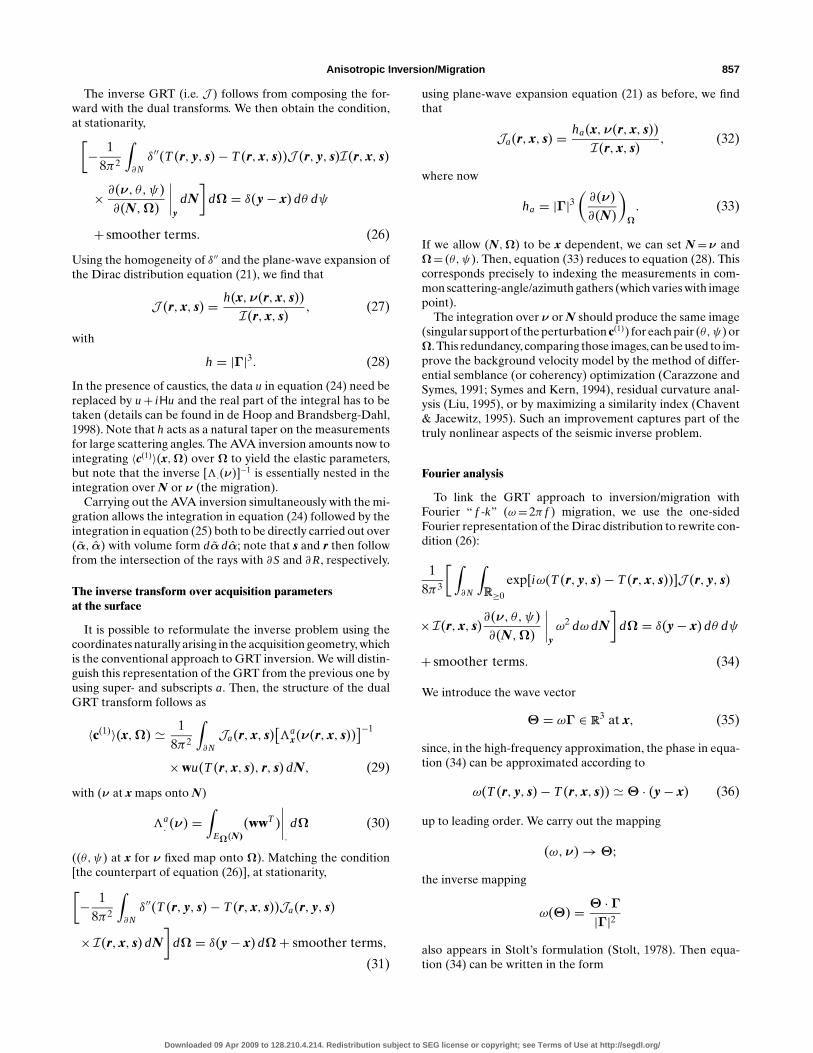
resolution kernel for a range of apertures. We note that thecomputer implementation of the theory given in the previoussections can be built around conventional Kirchhoff-type mi-gration software. In the first example, we reconstruct densityusing a finite aperture dataset and then carry out the analyticnormalization associated with the diagonal of the resolutionkernel. Datasets with limited scattering angles (θ) were drawnfrom a “complete” dataset with measurements taken at 10 000Hammersley-point distributed source-receiver pairs (de Hoopand Spencer, 1996, who showed that Hammersley points pro-duce accurate discretizations of the GRT). Each subset of datapreserved a full range of scattering azimuths and migrationdips, and involved at most 100 sources and 100 receivers. Theresults for the 3 computation are shown in Figure 2 and forthe full reconstruction of density in Table 4. We note that theestimates of density change by a factor of two as the scatteringangle aperture is increased from 22 to 180. The final columnof Table 4 shows the results of correcting the inversions usingthe maximum scattering angle. We have been able to recoverthe “correct” result to within 1% at all apertures.

Table 4. Tests of limiting scattering angles to within the rangeθ ∈ [0,θmax]. A full ν aperture was used with a point-densityperturbation. The correct answer is 1.6025 × 10−10 m. Thesecond column shows numerical results from a limited apertureevaluation of equation (58). The third column shows the resultsof correcting column 2 with the analytic expression for apertureequation (57).

θmax 〈ρ(1)〉/10−10 (8π 3/C)〈ρ(1)〉/10−10

88π 1.594 1.59468π 2.308 1.58458π 2.864 1.58848π 2.977 1.58638π 3.044 1.58728π 3.282 1.58918π 3.518 1.585

FIG. 2. The theoretical values of 3 for the case of a densityinversion with a homogeneous background (solid line) com-pared with those calculated using Hammersley points (dashedline).



The accuracy of the linearization assumption

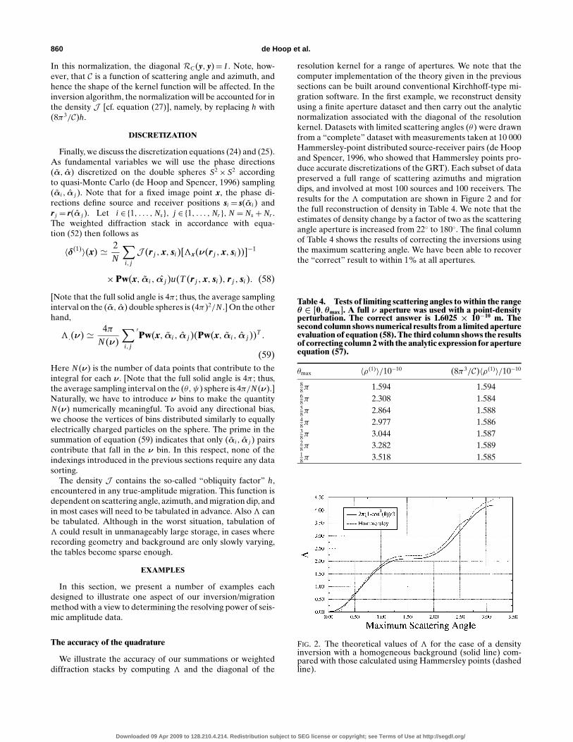
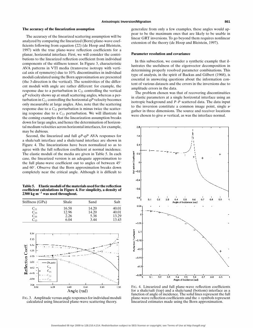
The accuracy of the linearized scattering assumption will beanalyzed by comparing the linearized (Born) plane-wave coef-ficients following from equation (22) (de Hoop and Bleistein,1997) with the true plane-wave reflection coefficients for aplanar, horizontal interface. First, we will consider the contri-butions to the linearized reflection coefficient from individualcomponents of the stiffness tensor. In Figure 3, characteristicAVA patterns in VTI media (transverse isotropy with verti-cal axis of symmetry) due to 10% discontinuities in individualmoduli calculated using the Born approximation are presented(the 3-direction is the vertical). The sensitivities of the differ-ent moduli with angle are rather different: for example, theresponse due to a perturbation in C33 controlling the verticalqP velocity shows up at small scattering angles, whereas a per-turbation in C11 controlling the horizontal qP velocity becomesonly measurable at large angles. Also, note that the scatteringresponse due to a C55 perturbation is minus twice the scatter-ing response due to a C13 perturbation. We will illustrate inthe coming examples that the linearization assumption breaksdown for large angles, and hence the determination of horizon-tal medium velocities across horizontal interfaces, for example,may be dubious.

Second, the linearized and full qP-qP AVA responses fora shale/salt interface and a shale/sand interface are shown inFigure 4. The linearizations have been normalized so as toagree with the full reflection coefficient at normal incidence.The elastic moduli of the media are given in Table 5. In eachcase, the linearized version is an adequate approximation tothe full plane-wave coefficient out to angles of between 45

and 60. Observe that the Born approximation breaks downcompletely near the critical angle. Although it is difficult to

Table 5. Elastic moduli of the materials used for the reflectioncoefficient calculations in Figure 4. For simplicity, a density of2300 kg m−3 was used throughout.

Stiffness (GPa) Shale Sand Salt

C11 16.58 14.20 40.01C33 12.96 14.20 40.01C55 2.26 5.38 13.29C13 6.04 3.44 13.43

FIG.3. Amplitude versus angle responses for individual modulicalculated using linearized plane-wave scattering theory.

generalize from only a few examples, these angles would ap-pear to be the maximum ones that are likely to be usable inlinear GRT inversions. To go beyond them requires nonlinearextension of the theory (de Hoop and Bleistein, 1997).

Parameter resolution and covariance

In this subsection, we consider a synthetic example that il-lustrates the usefulness of the eigenvector decomposition indetermining properly resolved parameter combinations. Thistype of analysis, in the spirit of Backus and Gilbert (1968), isessential in answering questions about the information con-tent of various datasets and the errors in the inversions due toamplitude errors in the data.

The problem chosen was that of recovering discontinuitiesin elastic parameters at a single horizontal interface using anisotropic background and P-P scattered data. The data inputto the inversion constitute a common image point, single νgather in three dimensions. The source and receiver locationswere chosen to give ν vertical, as was the interface normal.

FIG. 4. Linearized and full plane-wave reflection coefficientsfor a shale/salt (top) and a shale/sand (bottom) interface as afunction of angle of incidence. The solid lines represent the fullplane-wave reflection coefficients and the+ symbols representlinearized estimates made using the Born approximation.


862 de Hoop et al.

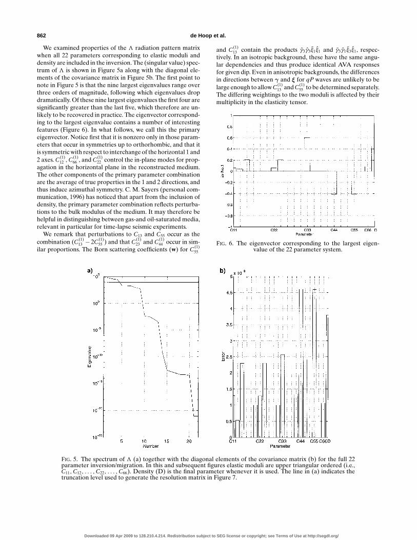
We examined properties of the 3 radiation pattern matrixwhen all 22 parameters corresponding to elastic moduli anddensity are included in the inversion. The (singular value) spec-trum of 3 is shown in Figure 5a along with the diagonal ele-ments of the covariance matrix in Figure 5b. The first point tonote in Figure 5 is that the nine largest eigenvalues range overthree orders of magnitude, following which eigenvalues dropdramatically. Of these nine largest eigenvalues the first four aresignificantly greater than the last five, which therefore are un-likely to be recovered in practice. The eigenvector correspond-ing to the largest eigenvalue contains a number of interestingfeatures (Figure 6). In what follows, we call this the primaryeigenvector. Notice first that it is nonzero only in those param-eters that occur in symmetries up to orthorhombic, and that itis symmetric with respect to interchange of the horizontal 1 and2 axes. C(1)

12 ,C(1)66 , and C(1)

22 control the in-plane modes for prop-agation in the horizontal plane in the reconstructed medium.The other components of the primary parameter combinationare the average of true properties in the 1 and 2 directions, andthus induce azimuthal symmetry. C. M. Sayers (personal com-munication, 1996) has noticed that apart from the inclusion ofdensity, the primary parameter combination reflects perturba-tions to the bulk modulus of the medium. It may therefore behelpful in distinguishing between gas-and oil-saturated media,relevant in particular for time-lapse seismic experiments.

We remark that perturbations to C13 and C55 occur as thecombination (C(1)

13 − 2C(1)55 ) and that C(1)

23 and C(1)44 occur in sim-

ilar proportions. The Born scattering coefficients (w) for C(1)55

FIG. 5. The spectrum of 3 (a) together with the diagonal elements of the covariance matrix (b) for the full 22parameter inversion/migration. In this and subsequent figures elastic moduli are upper triangular ordered (i.e.,C11,C12, . . . ,C22, . . . ,C66). Density (D) is the final parameter whenever it is used. The line in (a) indicates thetruncation level used to generate the resolution matrix in Figure 7.

and C(1)13 contain the products γ3γ3ξ1ξ1 and γ3γ1ξ3ξ1, respec-

tively. In an isotropic background, these have the same angu-lar dependencies and thus produce identical AVA responsesfor given dip. Even in anisotropic backgrounds, the differencesin directions between γ and ξ for qP waves are unlikely to belarge enough to allow C(1)

13 and C(1)55 to be determined separately.

The differing weightings to the two moduli is affected by theirmultiplicity in the elasticity tensor.

FIG. 6. The eigenvector corresponding to the largest eigen-value of the 22 parameter system.



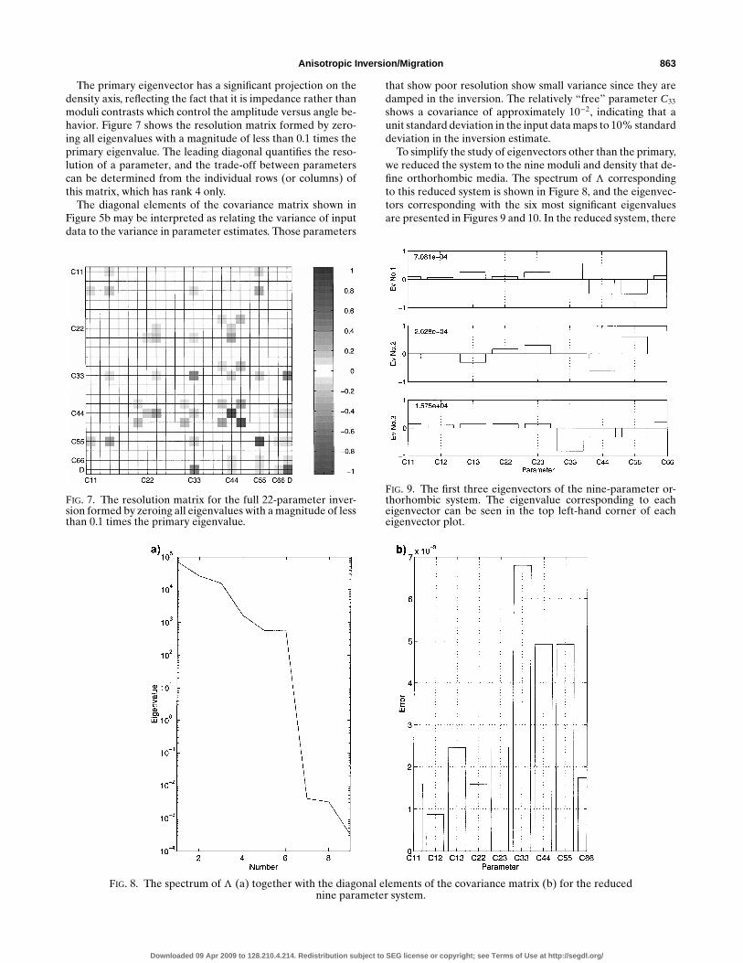
The primary eigenvector has a significant projection on thedensity axis, reflecting the fact that it is impedance rather thanmoduli contrasts which control the amplitude versus angle be-havior. Figure 7 shows the resolution matrix formed by zero-ing all eigenvalues with a magnitude of less than 0.1 times theprimary eigenvalue. The leading diagonal quantifies the reso-lution of a parameter, and the trade-off between parameterscan be determined from the individual rows (or columns) ofthis matrix, which has rank 4 only.

The diagonal elements of the covariance matrix shown inFigure 5b may be interpreted as relating the variance of inputdata to the variance in parameter estimates. Those parameters

FIG. 7. The resolution matrix for the full 22-parameter inver-sion formed by zeroing all eigenvalues with a magnitude of lessthan 0.1 times the primary eigenvalue.

FIG. 8. The spectrum of 3 (a) together with the diagonal elements of the covariance matrix (b) for the reducednine parameter system.

that show poor resolution show small variance since they aredamped in the inversion. The relatively “free” parameter C33

shows a covariance of approximately 10−2, indicating that aunit standard deviation in the input data maps to 10% standarddeviation in the inversion estimate.

To simplify the study of eigenvectors other than the primary,we reduced the system to the nine moduli and density that de-fine orthorhombic media. The spectrum of 3 correspondingto this reduced system is shown in Figure 8, and the eigenvec-tors corresponding with the six most significant eigenvaluesare presented in Figures 9 and 10. In the reduced system, there

FIG. 9. The first three eigenvectors of the nine-parameter or-thorhombic system. The eigenvalue corresponding to eacheigenvector can be seen in the top left-hand corner of eacheigenvector plot.


864 de Hoop et al.

are only six eigenvalues greater than 10−3 times the maximumeigenvalue.

The primary eigenvector in the reduced system is essen-tially the same as in the case of the full 22 parameter system(see Figure 6). The second eigenvector is interesting in thatit is antisymmetric with respect to interchange of the 1 and2 axes (Figure 9). Thus, linear combinations of the primaryeigenvector, which is symmetric with respect to interchange ofthe 1 and 2 axes, and the second eigenvector serve to definea “best resolved parameter combination” and “its azimuthalvariation.”

The determination of the vertical qP (C33) discontinuity be-comes possible when the third eigenvector is included. Eigen-vector 3 (Figure 9) is similar to the first except that the signof C(1)

33 is reversed. Thus, the difference of eigenvector 1 and 3isolates C(1)

33 , whereas the sum of 1 and 3 isolates the param-eters (C(1)

13 − 2C(1)55 ) and (C(1)

23 − 2C(1)44 ). These, in turn, may be

separated using eigenvector 2.Eigenvalues 4, 5, and 6 are more than a factor of 10 smaller

than eigenvector 3, but are interesting nevertheless. The eigen-vector corresponding to the fourth largest eigenvalue is shownin Figure 10. It is the first to show that the qP wave excites bothshear polarizations (C(1)

12 ,C(1)66 ) that takes place in the presence

of general anisotropy. Here, we note that its affects on AVAare due to the combination (C(1)

12 + 2C(1)66 ). Eigenvectors 5 and

6 contain linear combinations of the two horizontal velocityparameters C(1)

11 and C(1)22 and, taken together, isolate these two

velocities individually.One may wonder how the reconstructed linear parameter

combinations relate to the nonlinear combinations appearingin the more conventional AVA analysis. The latter analysis pro-vides an expansion with scattering angle/azimuth, the coeffi-cients of which are particular combinations of moduli. Thosecombinations can be linearized in perturbations of stiffness,yielding vectors that span a linear subspace of medium param-eters. Loosely speaking, this subspace appears to be reachableby our GRT inversion approach. Note in this respect that with

FIG. 10. The second 3 eigenvectors of the 9 parameter or-thorhombic system. The eigenvalue corresponding to eacheigenvector can be seen in the top left-hand corner of eacheigenvector plot.

the GRT, we combine (integrate) reflection data over a rangeof scattering angles/azimuths.

We have carried out similar tests using qP waves in aniso-tropic backgrounds and different dips. In principle, an isotropicbackground makes only a small difference. Its effects on theradiation pattern matrix are confined to a lack of parallelismof the polarization and slowness vectors plus changes to phaseangle at the image point. The effect of anisotropy on qS waves,though, will be large since their polarizations can vary morestrongly.

Varying migration dip has two important effects. For agiven sampling of the scattering angle sphere and assumingan isotropic background, the parameter combinations that aredetermined from a gather rotate with the migration dip ν. Asan example, in Figure 11 the resolution matrix is shown for aconfiguration in which the dip is 45 and which is recorded withangles of incidence of up to 45 with respect to ν. Note how theproblem becomes symmetrical with respect to interchange ofthe 1 and 3 axes while the 1–2 symmetries and antisymmetriesdiscussed above are destroyed. The rank of the system is notchanged by the rotation. A second effect of introducing migra-tion dip is that, for a given recording geometry, the range ofscattering angles reached is dip dependent. For example, in anisotropic background at a dip of 45 (in plane), the maximumscattering angle associated with a recording at the surface is 90.Constraining the maximum recording angle at the image pointto 60 the maximum scattering angle reduces to 30. In thiscase, the rank of the system and hence resolution is seriouslydegraded. In Figure 12, the spectrum of3 using this restrictedaperture is shown. For all practical purposes, the rank of thesystem is reduced to 1, and all that can be determined is animpedance associated with propagation at approximately 45.

Spatial resolution

In this subsection, we carry out more complete tests designedto show the antialiasing benefits of GRT and quasi–MonteCarlo sampling methods, and the improved spatial resolutionthat can be obtained at the expense of degrading parameter

FIG. 11. The resolution matrix of the full 22-parameter systemusing a migration dip of 45 and incident angles of up of 45.Compare Figure 7.



resolution. The tests are illustrated in Figures 13–16 and willbe explained below. Comparisons of GRT inversions withKirchhoff migrations in the isotropic case have been given pre-viously. Dillon (1990) presents one such comparison and pointsout the antialiasing properties of the GRT operator. Similar ar-guments apply in the anisotropic case.

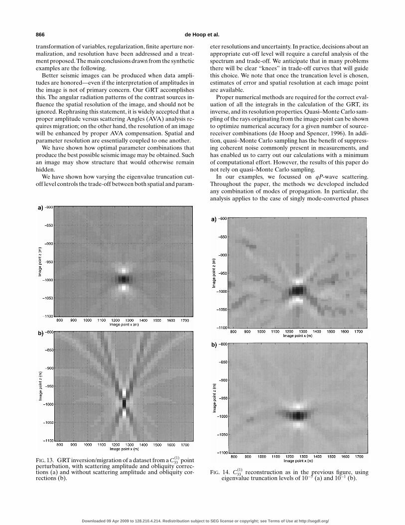
We considered a 3500-m recording aperture and calculatedseismograms for a point perturbation to C33 at a depth of1000 m, and carried out the inversion. To illustrate the an-tialiasing effects of the GRT, we used a line, centered over thescatterer, of 251 coincident sources and receivers having a 10-mspacing. Images both with and without the inclusion of radia-tion pattern in the inversion are presented in Figure 13. Notehow strongly the scattering amplitudes affect the edge effectseen in Figure 13. (Note also that, since the data are zero off-set, the obliquity factor is a constant and does not affect theseresults.)

The spatial resolution operator contains the pseudoinverseof 3 and, hence, there is a relationship between parameterresolution and spatial resolution. The next example illustratesthis relationship, again for the case of a point perturbationto C33. Synthetic data were generated for 2000 Hammersleydistributed source-receiver pairs within horizontal distancesof 1000 m from a scatterer at 1000 m depth. Figure 14 showsa comparison of the effects of different eigenvalue truncationlevels on the image. The higher truncation level (Figure 14b)improves the migration impulse response, although it has theeffect of degrading parameter resolution.

In the next examples, we have carried out full multipa-rameter inversions of two different synthetic datasets. Thefirst dataset is the scattered field due to two point perturba-

FIG. 12. The eigenvalue spectrum of the 22-parameter system obtained using a dip of 45. Propagation angles ofup to 60 from the vertical were used corresponding to a maximum scattering angle of 30. Compare Figure 5.

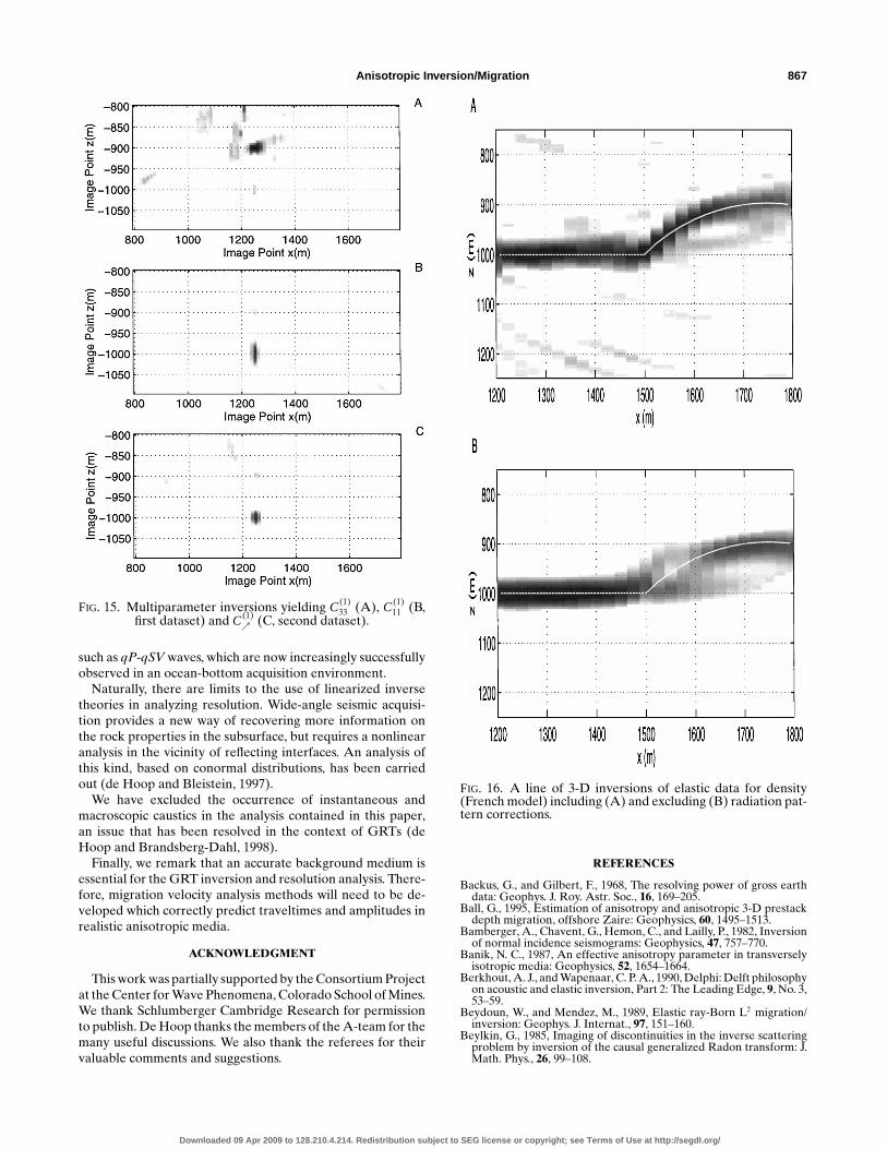
tions: C33 at a depth of 900 m and C11 at a depth of 1000 m(common horizontal coordinate of 1250 m). Results of theinversion of this dataset are shown in Figure 15a (C33) andFigure 15b (C11). Our algorithm provides automatically sucha multiple set of images. In the second dataset, the pointperturbation to C11 was replaced by a point perturbation toC = [C11+C33+ 2(C13+ 2C55)]/4, an approximation to the45 qP-wave slowness. The result of inverting the seconddataset for C is given in Figure 15c. In Figure 15, the grayscale covers the same range of absolute amplitudes and a fullscattering aperture was synthesized. Note that the separationof parameters from both datasets is satisfactory. The imperfec-tions in the C33 image (Figure 15a) are caused by using quasi–Monte Carlo source-receiver locations optimized for the in-version at a depth of 1000 m, rather than the actual depth of900 m. As a final demonstration of improved spatial resolution,a 3-D inversion was carried out for the model seen in Figure 16.Hammersley-distributed sources and receivers were used anda single parameter, density, was perturbed. Elastic qP-wavedata were generated over the structure using a Kirchhoff inte-gration technique. The improvements obtained using the fullGRT algorithm illustrate that elastic data should be treatedas such. Note particularly how the uniform density contrastat the “dome” is properly determined using a GRT inversion(Figure 16A) but deteriorates when the AVA factors are ig-nored (Figure 16B).

CONCLUSIONS

In this paper, we have presented a method for carryingout inversion/migration in anisotropic media using the gen-eralized Radon transform (GRT). Practical aspects, such as


866 de Hoop et al.

transformation of variables, regularization, finite aperture nor-malization, and resolution have been addressed and a treat-ment proposed. The main conclusions drawn from the syntheticexamples are the following.

Better seismic images can be produced when data ampli-tudes are honored—even if the interpretation of amplitudes inthe image is not of primary concern. Our GRT accomplishesthis. The angular radiation patterns of the contrast sources in-fluence the spatial resolution of the image, and should not beignored. Rephrasing this statement, it is widely accepted that aproper amplitude versus scattering Angles (AVA) analysis re-quires migration; on the other hand, the resolution of an imagewill be enhanced by proper AVA compensation. Spatial andparameter resolution are essentially coupled to one another.

We have shown how optimal parameter combinations thatproduce the best possible seismic image may be obtained. Suchan image may show structure that would otherwise remainhidden.

We have shown how varying the eigenvalue truncation cut-off level controls the trade-off between both spatial and param-

FIG. 13. GRT inversion/migration of a dataset from a C(1)33 point

perturbation, with scattering amplitude and obliquity correc-tions (a) and without scattering amplitude and obliquity cor-rections (b).

eter resolutions and uncertainty. In practice, decisions about anappropriate cut-off level will require a careful analysis of thespectrum and trade-off. We anticipate that in many problemsthere will be clear “knees” in trade-off curves that will guidethis choice. We note that once the truncation level is chosen,estimates of error and spatial resolution at each image pointare available.

Proper numerical methods are required for the correct eval-uation of all the integrals in the calculation of the GRT, itsinverse, and its resolution properties. Quasi–Monte Carlo sam-pling of the rays originating from the image point can be shownto optimize numerical accuracy for a given number of source-receiver combinations (de Hoop and Spencer, 1996). In addi-tion, quasi–Monte Carlo sampling has the benefit of suppress-ing coherent noise commonly present in measurements, andhas enabled us to carry out our calculations with a minimumof computational effort. However, the results of this paper donot rely on quasi–Monte Carlo sampling.

In our examples, we focussed on qP-wave scattering.Throughout the paper, the methods we developed includedany combination of modes of propagation. In particular, theanalysis applies to the case of singly mode-converted phases

FIG. 14. C(1)33 reconstruction as in the previous figure, using

eigenvalue truncation levels of 10−5 (a) and 10−1 (b).



FIG. 15. Multiparameter inversions yielding C(1)33 (A), C(1)

11 (B,first dataset) and C(1)

(C, second dataset).

such as qP-qSV waves, which are now increasingly successfullyobserved in an ocean-bottom acquisition environment.

Naturally, there are limits to the use of linearized inversetheories in analyzing resolution. Wide-angle seismic acquisi-tion provides a new way of recovering more information onthe rock properties in the subsurface, but requires a nonlinearanalysis in the vicinity of reflecting interfaces. An analysis ofthis kind, based on conormal distributions, has been carriedout (de Hoop and Bleistein, 1997).

We have excluded the occurrence of instantaneous andmacroscopic caustics in the analysis contained in this paper,an issue that has been resolved in the context of GRTs (deHoop and Brandsberg-Dahl, 1998).

Finally, we remark that an accurate background medium isessential for the GRT inversion and resolution analysis. There-fore, migration velocity analysis methods will need to be de-veloped which correctly predict traveltimes and amplitudes inrealistic anisotropic media.

ACKNOWLEDGMENT

This work was partially supported by the Consortium Projectat the Center for Wave Phenomena, Colorado School of Mines.We thank Schlumberger Cambridge Research for permissionto publish. De Hoop thanks the members of the A-team for themany useful discussions. We also thank the referees for theirvaluable comments and suggestions.

FIG. 16. A line of 3-D inversions of elastic data for density(French model) including (A) and excluding (B) radiation pat-tern corrections.

REFERENCES

Backus, G., and Gilbert, F., 1968, The resolving power of gross earthdata: Geophys. J. Roy. Astr. Soc., 16, 169–205.

Ball, G., 1995, Estimation of anisotropy and anisotropic 3-D prestackdepth migration, offshore Zaire: Geophysics, 60, 1495–1513.

Bamberger, A., Chavent, G., Hemon, C., and Lailly, P., 1982, Inversionof normal incidence seismograms: Geophysics, 47, 757–770.

Banik, N. C., 1987, An effective anisotropy parameter in transverselyisotropic media: Geophysics, 52, 1654–1664.

Berkhout, A. J., and Wapenaar, C. P. A., 1990, Delphi: Delft philosophyon acoustic and elastic inversion, Part 2: The Leading Edge, 9, No. 3,53–59.

Beydoun, W., and Mendez, M., 1989, Elastic ray-Born L2 migration/inversion: Geophys. J. Internat., 97, 151–160.

Beylkin, G., 1985, Imaging of discontinuities in the inverse scatteringproblem by inversion of the causal generalized Radon transform: J.Math. Phys., 26, 99–108.


868 de Hoop et al.

Beylkin, G., and Burridge, R., 1990, Linearized inverse scattering prob-lem of acoustics and elasticity: Wave Motion, 12, 15–52.

Bleistein, N., 1987, On the imaging of reflectors within the earth: Geo-physics, 52, 931–942.

Bleistein, N., and Cohen, J. K., 1979, Direct inversion procedure forClaerbout’s equation: Geophysics, 44, 1034–1040.

Burridge, R., de Hoop, M. V., Miller, D., and Spencer, C., 1998, Multipa-rameter inversion in anisotropic elastic media: Geophys. J. Internat.,134, 757–777.

Campbell, S., and Meyer, C., 1979, Generalized inverses of linear trans-formations: Pitman.

Cao, D., Beydoun, W. B., Singh, S. C., and Tarantola, A., 1990, A si-multaneous inversion for background velocity and impedance maps:Geophysics, 55, 458–469.

Carazzone, J. J., and Symes, W. W., 1991, Velocity inversion by differ-ential semblance optimization: Geophysics, 56, 654–663.

Chavent, G., and Jacewitz, C. A., 1995, Determination of backgroundvelocities by multiple migration fitting: Geophysics, 60, 476–490.

Cheng, G., and Coen, S., 1984, The relationship between Born inver-sion and migration for common-midpoint stacked data: Geophysics,49, 2117–2131.

Claerbout, J. F., 1992. Earth sounding analysis: Processing versus in-version: Blackwell Scientific Publications.

Clayton, R. W., and Stolt, R. H., 1981, A Born-WKBJ inversion methodfor acoustic reflection data: Geophysics, 46, 1559–1567.

Debski, W., and Tarantola, A., 1995, Information on elastic parame-ters obtained from the amplitudes of reflected waves: Geophysics,60, 1426–1436.

de Hoop, M. V., and Bleistein, N., 1997, Generalized Radon transforminversions for reflectivity in anisotropic elastic media: Inverse Prob-lems, 13, 669–690.

de Hoop, M. V., and Brandsberg-Dahl, S., 1998, Maslov asymptoticextension of generalized Radon transform inversions in anisotropicelastic media: A least-squares approach, in Seismic imaging; lecturenotes of the 1998 Mathematical Geophysics Summer School at Stan-ford University: Soc. Ind. Appl. Math.

de Hoop, M. V., and de Hoop, A. T., 1997, Wavefield reciprocity andlocal optimization in remote sensing: Center for Wave Phenomena,Colorado School of Mines, preprint 242.

de Hoop, M. V., and Spencer, C., 1996, Quasi–Monte Carlo integra-tion over S2 × S2 for migration × inversion: Inverse Problems, 12,219–239.

de Hoop, M. V., Burridge, R., Spencer, C., and Miller, D., 1994, Gener-alized Radon transformation/amplitude versus angle (GRT/AVA)migration/inversion in anisotropic media, in Hassanzadeh, S., Ed.,Proc. SPIE 2301, 15–27.

Devaney, A. J., 1984, Geophysical diffraction tomography: IEEE Trans.Geosci. Remote Sensing, GE-22, 3–13.

Dillon, P. B., 1990, A comparison between Kirchhoff and GRT migra-tion on VSP data: Geophys. Prosp., 38, 757–777.

Eaton, D. W. S., and Stewart, R. R., 1994, Migration/inversion fortransversely isotropic elastic media: Geophys. J. Internat., 119, 667–683.

Esmersoy, C., and Oristaglio, M., 1988, Reverse-time wave-field ex-trapolation imaging and inversion: Geophysics, 53, 920–931.

Gauthier, O., Virieux, J., and Tarantola, A., 1986, Two-dimensionalnonlinear inversion of seismic waveforms—Numerical results: Geo-physics, 51, 1387–1403.

Hornby, B. E., Schwartz, L. M., and Hudson, J. A., 1994, Anisotropiceffective medium modeling of the elastic properties of shales: Geo-physics, 59, 1570–1583.

Ikelle, L. T., Diet, J. P., and Tarantola, A., 1986, Linearized inversionof multioffset seismic reflection data in the frequency-wavenumberdomain: Geophysics, 51, 1266–1276.

Jin, S., Madariaga, R., Virieux, J., and Lambare, G., 1992, Two-dimen-sional asymptotic iterative elastic inversion: Geophys. J. Internat.,108, 575–588.

Kendall, J.-M., Guest, W. S., and Thomson, C. J., 1992, Ray-theoryGreen’s function reciprocity and ray centered coordinates inanisotropic media. Geophys. J. Internat., 108, 364–371.

Larner, K., and Tsvankin, I., 1995, P-wave anisotropy: Its practicalestimation and importance in processing and interpretation of seis-mic data. 65th Ann. Internat. Mtg. Soc. Expl. Geophys., ExpandedAbstracts, 1502–1505.

Liu, Z., 1995, Migration velocity analysis: Center for Wave Phenom-ena, Colorado School of Mines, preprint 168.

Miller, D., Oristaglio, M., and Beylkin, G., 1987, A new slant on seismicimaging: Migration and integral geometry: Geophysics, 52, 943–964.

Mora, P., 1989, Inversion = migration + tomography: Geophysics, 54,1575–1586.

Norton, S. G., and Linzer, M., 1981, Ultrasonic scattering potentialimaging in three dimensions: Exact inverse scattering solutions forplane, cylindrical, and spherical apertures. IEEE Trans. BiomedicalEng., BME-28, 202–220.

Ruger, A., 1996, Variation of P-wave reflectivity with offset and az-imuth in anisotropic media: Center for Wave Phenomena, ColoradoSchool of Mines, preprint 218.

Shearer, P. M., and Chapman, C. H., 1989, Ray tracing in azimuthallyanisotropic media—I. Results for models of aligned cracks in theupper crust: Geophys. J., 96, 51–64.

Singh, S. C., West, G. F., Bregman, N. D., and Chapman, C. H., 1989, Fullwaveform inversion of reflection data: J. Geophys. Res., 94, 1777–1794.

Snieder, R., Xie, M. Y., Pica, A., and Tarantola, A., 1989, Retreiv-ing both the impedance contrast and background velocity: A globalstrategy for the seismic reflection problem: Geophysics, 54, 991–1000.

Stolt, R. H., 1978, Migration by Fourier transform: Geophysics, 43,23–48.

Symes, W. W., and Kern, M., 1994, Inversion of reflection seismo-grams by differential semblance analysis: Algorithm structure andsynthetic examples. Geophys. Prosp., 42, 565–614.

Tarantola, A., 1984, Inversion of seismic reflection data in the acousticapproximation: Geophysics, 49, 1259–1266.

——— 1986, A strategy for nonlinear elastic inversion of seismic re-flection data: Geophysics, 51, 1893–1903.

Thomsen, L., 1986, Weak elastic anisotropy: Geophysics, 51, 1954–1966.

Tsvankin, I., and Thomsen, L., 1995, Inversion of reflection traveltimesfor transverse isotropy: Geophysics, 60, 1095–1107.

APPENDIX A

∂(α, α)/∂(ν, θ,ψ) IN GENERAL MEDIA

We have

ν = λ(α, α)α+ µ(α, α)α, (A-1)

where [cf. equation (19)]

λ = |γ||Γ| , µ = |γ||Γ| . (A-2)

Note that

α ∈ S2, α ∈ S2, and ν ∈ S2. (A-3)

We introduce the angle θ between the unite phase directionsas

cos θ = α · α, θ ∈ [0, π). (A-4)

In view of equation (A-3), we have the constraint

λ2 + µ2 + 2 λµ cos θ = 1. (A-5)

Further, we introduce the unit vector

ζ = 1sin θ

(α ∧ α) ∧ ν = (α · ν)α− (α · ν)αsin θ

. (A-6)

[Note that (α ·ν)= λ+µ cos θ while (α ·ν)= λ cos θ +µ.] Thevectors α, α,ν, and ζ lie in the same plane; also ζ⊥ν. Notethat for ν fixed, ζ ∈ S1. We shall analyse the transformation(α, α)→ (ν, θ, ψ), whereψ denotes the angular displacement(azimuth) of ζ, and evaluate the associated Jacobian.

First, let α and α vary in their own plane [(1, 3) coordinates,i.e., the plane they initially span] keeping ψ fixed. The associ-ated infinitesimal angular displacements of the relevant vectors



will be denoted by the superscript‖. Then, in terms of anglesu, v in a fixed reference frame, we write

α =

sin u

0

cos u

, ∂uα =

cos u

0

−sin u

,(A-7)

α =

sin v

0

cos v

, ∂vα =

cos v

0

−sin v

,while λ= λ(u, v) and µ=µ(u, v). Note that

v − u = θ. (A-8)

In general, from equations (A-1) and (A-7), it follows that forin-plane variations,

dν = (∂uλdu+ ∂vλdv)α+ λ∂uαdu

+ (∂uµdu+ ∂vµdv)α+ µ∂vαdv. (A-9)

We introduce the unit vector [cf. equation (A-5)]

ν ′ = λ(u, v)∂uα + µ(u, v)∂vα. (A-10)

Note that

∂uα⊥ α, ∂vα⊥ α, ν ′ ⊥ν, (A-11)

while α, ∂uα, α, ∂vα,ν, and ν ′ all lie in the same plane.Since ν · dν = 0, the angular displacement dν‖ of ν is given

by

dν‖ = ν ′ · dν = [λ2 + λ(∂uµ)(∂uα · α)

+µ(∂uλ)(α · ∂vα)+ λµ(∂uα · ∂vα)]

du

+ [λµ(∂uα · ∂vα)+ λ(∂vµ)(∂uα · α)

+µ(∂vλ)(α · ∂vα)+ µ2]dv. (A-12)

On the other hand, using equation (A-8),

dθ = dv − du. (A-13)

In our notation, the angular displacement of the phase direc-tions are dα‖ =du and dα‖ =dv. Combining equations (A-12)and (A-13), using equation (A-7) leads to the Jacobian

∂(ν‖, θ)∂(u, v)

=∣∣∣∣λ2 + (λ∂uµ− (∂uλ)µ) sin θ + λµ cos θ µ2 + (λ∂vµ− (∂vλ)µ) sin θ + λµ cos θ

−1 1

∣∣∣∣= λ2 + µ2 + 2λµ cos θ + [λ(∂uµ+ ∂vµ)− (∂uλ+ ∂vλ)µ] sin θ. (A-14)

Using equation (A-5), this results in

∂(ν‖, θ)

∂(α‖, α‖)= 1+ λµ

[(∂u + ∂v) log

(µ

λ

)]sin θ. (A-15)

Secondly, consider the case where α and α are varied per-pendicular to the plane they initially span. The associated in-finitesimal angular displacements of the relevant vectors willbe denoted by the superscript⊥. The out-of-plane variations,keeping θ fixed, imply

dζ, dν ∼

0

1

0

. (A-16)

To evaluate the out-of-plane Jacobian, it will be convenient tointroduce angles θ , θ according to

cos θ = α · ν, cos θ = α · ν. (A-17)

Note that

θ + θ = θ. (A-18)

Then [cf. equation (A-6)],

ζ = cos θα− cos θαsin θ

. (A-19)

The sine rule applied to the triangle made up of the threevectors λα, µα, and ν gives

sin θµ= sin θ

λ= sin θ. (A-20)

Substituting equation (A-20) into equation (A-1) yields

ν = sin θα+ sin θαsin θ

. (A-21)

The angular displacement of ν, using constraint (A-16), is thengiven by

dν⊥ = sin θ dα⊥ + sin θdα⊥

sin θ. (A-22)

On the other hand, from equation (A-19) directly follows that

dζ⊥ = cos θ dα⊥ − cos θ dα⊥

sin θ. (A-23)

Note that dζ⊥ =dψ . Combining equations (A-22) and (A-23)yields

∂(ν⊥, ζ⊥)

∂(α⊥, α⊥)= 1

sin2 θ

∣∣∣∣ sin θ sin θ

−cos θ cos θ

∣∣∣∣ = 1sin θ

. (A-24)


870 de Hoop et al.

Putting equations (A-15) and (A-24) together, we get

∂(ν, θ, ψ)∂(α, α)

= ∂(ν‖, θ)

∂(α‖, α‖)∂(ν⊥, ζ⊥)

∂(α⊥, α⊥)

=1+ λµ

[(∂u + ∂v) log

(µ

λ

)]sin θ

sin θ. (A-25)

Thus,

∂(α, α)∂(ν, θ, ψ)

= sin θ

1+ λµ[

(∂u + ∂v) log(µ

λ

)]sin θ

.

(A-26)

In this final expression, we can substitute [cf. equation (A-2)]

µ

λ= |γ||γ| =

V(α(u))

V(α(v)), (A-27)

where V denotes the phase velocity as before, and so

(∂u + ∂v) log(µ

λ

)= −∂u log|γ| + ∂v log|γ|. (A-28)

Here,

∂u log |γ| = ∂u|γ||γ| = tan χ with cos χ = n‖ . α,

(A-29)

∂v log |γ| = ∂v|γ||γ| = tan χ with cos χ = n‖ · α.

(A-30)

Note that n‖, n‖ are determined by ψ ; we have χ = χ(ψ) andχ = χ(ψ).

APPENDIX B

∂(ν)/∂(N) IN AN ISOTROPIC MEDIUM

In the main text of this paper, Beylkin’s determinant wasexpressed as [cf. equation (48)]


) = Γ · (∂N1Γ ∧ ∂N2Γ). (B-1)

Substituting equation (16) (Γ= γ+ γ) into equation (B-1)yields a separation into source and receiver ray geometry,


) = (γ + γ) · (∂N1 γ ∧ ∂N2 γ

+ ∂N1 γ ∧ ∂N2 γ + ∂N1 γ ∧ ∂N2 γ + ∂N1 γ ∧ ∂N2 γ).

(B-2)

Let the background medium be homogeneous. Then, the raysconnecting the source at s and the receiver at r with the imagepoint y coincide with the vectors

R = y− s, R = y− r, (B-3)

respectively. In an isotropic medium, the phase and group di-rections coincide, hence [cf. equation (13)]

α = R|R| , α = R

|R| . (B-4)

Also, in equation (14),

V = V = c (B-5)

is angle independent.In order to evaluate ∂N1 γ, we carry out some side calcula-

tions [see also equation (49)]. Let i1, i2, i3 denote the threebase vectors of a Cartesian reference frame. We have

2|R|∂sj |R| = ∂sj |R|2= ∂sj [(y−s) · (y−s)]=−2(y−s) · i j ;hence,

∂sj |R| = −α · i j . (B-6)

Using this result in differentiating γ= c−1α [cf. equation (8)],we obtain

∂sj γ = −[i j − (α · i j )α]

|R|c . (B-7)

In a likewise manner, we find that

∂r j γ = −[i j − (α · i j )α]

|R|c . (B-8)

Now, we consider the planar acquisition geometry [cf. equa-tion (18)],

s3 = 0; s1,2 = N1,2 −Ä1,2, ∂N1,2s = i1,2,

r3 = 0; r1,2 = N1,2 +Ä1,2, ∂N1,2r = i1,2.(B-9)

Then, with equations (B-7) and (B-8), we get

∂N1,2 γ = −[i1,2 − (α · i1,2)α]

|R|c ,

(B-10)

∂N1,2 γ = −[i1,2 − (α · i1,2)α]

|R|c .

Observe that

|i1,2 − (α · i1,2)α| = [1− (α · i1,2)2]1/2,

|i1,2 − (α · i1,2)α| = [1− (α · i1,2)2]1/2,

while

[i1 − (α · i1)α] ∧ [i2 − (α · i2)α] = (α · i3)α,

and

[i1 − (α · i1)α] ∧ [i2 − (α · i2)α] = (α · i3)α.

We will substitute expressions (B-10) into equation (B-2).Equation (B-2) splits into eight contributions. To show thestructure of each contribution, consider the one,

γ · (∂N1 γ ∧ ∂N2 γ) = 1

c3

1

|R|1

|R|× α · [i1 − (α · i1)α] ∧ [i2 − (α · i2)α], (B-11)



with

α · [i1 − (α · i1)α] ∧ [i2 − (α · i2)α]

= det(α i1 − (α · i1)α i2 − (α · i2)α).

We have

det(α i1 − (α · i1)α i2 − (α · i2)α)

= det(α i1 i2) = (α · i3), (B-12)

det(α i1 − (α · i1)α i2 − (α · i2)α)

= (α · α) det(α i1 − (α · i1)α i2 − (α · i2)α)

= (α · α)(α · i3), (B-13)

det(α i1 − (α · i1)α i2 − (α · i2)α)

= det(α i1 i2 − (α · i2)α) = (α · i2)(α · i2)(α · i3)

+ [1− (α · i2)2](α · i3), (B-14)

det(α i1 − (α · i1)α i2 − (α · i2)α)

= det(α i1 − (α · i1)α i2) = [1− (α · i1)2](α · i3)

+ (α · i1)(α · i1)(α · i3), (B-15)

det(α i1 − (α · i1)α i2 − (α · i2)α)

= det(α i1 − (α · i1)α i2) = (α · i1)(α · i1)(α · i3)

+ [1− (α · i1)2](α · i3), (B-16)

det(α i1 − (α · i1)α i2 − (α · i2)α)

= det(α i1 i2 − (α · i2)α) = [1− (α · i2)2](α · i3)

+ (α · i2)(α · i2)(α · i3), (B-17)

det(α i1 − (α · i1)α i2 − (α · i2)α)

= det(α i1 i2) = (α · i3), (B-18)

det(α i1 − (α · i1)α i2 − (α · i2)α)

= (α · α) det(α i1 − (α · i1)α) i2 − (α · i2)α)

= (α · α)(α · i3). (B-19)

We have

equation (B-12)+ equation (B-13)

= [1+ (α · α)](α · i3), (B-20)


= (α · i3)+ (α · α)(α · i3), (B-21)


= (α · i3)+ (α · α)(α · i3), (B-22)


= [1+ (α · α)](α · i3). (B-23)

In view of the planar acquisition geometry, we have

(α · i3) = |R‖R|−1(α · i3). (B-24)

Hence, adding all the terms from equations (B-20)–(B-23) to-gether in accordance with equation (B-2) and with the properweighting with powers of |R| and |R|, we finally arrive at


)= (|R| + |R|)(|R|2 + |R|2)

|R|2|R|3[1+ (α · α)](α · i3)

c3.

(B-25)

On the other hand,

|Γ|3 = (2[1+ (α · α)])3/2

c3, (B-26)

so that

∂(ν)∂(N)

= (|R| + |R|)(|R|2 + |R|2)

|R|2|R|3|(α · i3)|

23/2[1+ (α · α)]1/2.

(B-27)

APPENDIX C

∂(c)/∂(δ1, . . . , δµ) FOR DEM

In this appendix, we derive a possible microstructure-drivenreparameterization of the medium perturbation. This param-eterization follows differential effective medium (DEM) the-ory combined with the self-consistent approximation. For adetailed discussion on this subject, see Hornby et al., (1994).The idea is that the medium may be perturbed by adding orsubtracting some generic rock-type material.

Basic volume averaging

Let a medium be composed of N constituents which occupyvolumes Vn, respectively. Constituents can be generic sandsand shales, for example. In the analysis, we consider a small

(compared to the wave length) sample volume V of compos-ite material. Let the constituent volume fractions be given byφn=Vn/V .

Volume averages of the strain ei j and the stress σpq are in-troduced through

〈ei j 〉 = 1V

∫V

ei j (x) dx, eni j =

1Vn

∫Vn

ei j (x) dx,

(C-1)

〈σpq〉 = 1V

∫Vσpq(x) dx, σ n

pq =1Vn

∫Vn

σpq(x) dx.


872 de Hoop et al.

Let si jpq denote a compliance tensor. We impose two constitu-tive laws, a macroscopic one,

〈ei j 〉 = s∗i j pq〈σpq〉, (C-2)

which yields the effective medium, and one for the constituentmedia,

eni j = sn

i jpq σnpq, (C-3)

valid in each inclusion. Let1i j pq denote the elastic unit tensor.Then,

sni jpqcn

pqk = 1i jk` (C-4)

describes the relation between the compliance and stiffnesstensors.

Now, since

〈ei j 〉 = 1V

N∑n=0

∫Vn

ei j (x) dx =N∑

n=0

φneni j

〈σpq〉 = 1V

N∑n=0

∫Vn

σpq(x) dx =N∑

n=0

φnσnpq,

(C-5)

we can analyse the change of compliance tensor, s∗i j pq − s0i j pq ,

under adding inclusions of media of type n= 1, . . . , N to a hostof type n= 0. Using both constitutive laws, we get

c0rsi j

(s0i j pq − s∗i j pq

)〈σpq〉 =N∑

n=1

φn(cn

rsi j − c0rsi j

)en

i j . (C-6)

To arrive at an expression for the constitutive parameters alone,the average strain en

i j in each inclusion is related to the suppos-edly uniform applied stress 〈σpq〉 on the outer boundary of oursample with volume V , namely,

eni j = Sn

i jpq〈σpq〉. (C-7)

The latter compliance tensor is unknown and may be com-plicated to compute (in the actual composite medium). Sub-stituting equation (C-7) into equation (C-6) eliminates 〈σpq〉and amounts to the explicit relationship between constitutivetensors:

s∗i j pq − s0i j pq = −s0

i jrs

N∑n=1

φn(cn

rsk` − c0rsk`

)Sn

k`pq. (C-8)

In terms of stiffnesses, the relation between the host and effec-tive medium tensors,

c∗i j pq − c0i j pq =

N∑n=1

φn(cn

i jrs − c0i jrs

)Sn

rsk`c∗k`pq, (C-9)

is not explicit.

Differential effective medium (DEM)

We discuss two implications of equations (C-8) and (C-9).First, removing the preference for the host medium, namely,replacing constituent n= 0 by the (yet to be determined) effec-

tive medium (c0i j pq → c∗i j pq), implies the system of equations

N∑n=1

φn(cn

i jrs − c∗i jrs

)Sn

rsk` = 0, (C-10)

from which Sni jpq can be solved in terms of c∗i jrs .

Second, it leads to the introduction of DEM theory. Let usconsider the case N= 1. The change1V1 in V1 will be assumedto be small. In general, we have

1φ1

φ1= 1V1

V1− 1V

V;

however, to preserve the amounts of other constituents we set1V =1V1. Hence,

1φ1

φ1= 1V1

V1

(1φ1− 1

)or

1V1

V= 1φ1

1− φ1. (C-11)

Substituting equation (C-11) into equations (C-8) and (C-9),and identifying

s0i j pq = s∗i j pq(φ1), c0

i j pq = c∗i j pq(φ1),(C-12)

s∗i j pq = s∗i j pq(φ1 +1φ1), c∗i j pq = c∗i j pq(φ1 +1φ1),

while

S1i j pq = S1

i j pq(φ1 +1φ1), (C-13)

we obtain

s∗i j pq(φ1 +1φ1)− s∗i j pq(φ1)

1φ1= − 1

1− φ1s∗i jrs (φ1)

× (c1rsk` − c∗rsk`(φ1)

)S1

k`pq(φ1 +1φ1) (C-14)

and

c∗i j pq(φ1 +1φ1)− c∗i j pq(φ1)

1φ1= 1

1− φ1

(c1

i jrs

− c∗i jrs (φ1))S1

rsk`(φ1 +1φ1)c∗k`pq(φ1 +1φ1). (C-15)

The DEM approximation amounts to neglecting 1φ1 in theright-hand sides of equations (C-14) and (C-15). In the con-text of GRT inversion/migration, the tensors s∗i j pq(φ1) andc∗i j pq(φ1) correspond with the anisotropic background velocitymodel.

Self consistent approximation

The question remains how to interpret the tensor Sni jpq . In

the self-consistent approximation, the tensor Sni jpq , dependent

on the actual composition of medium constituents everywherein the sample, is replaced by a tensor Sn,∗

i j pq that follows fromthe constitutive relation between strain and applied stress in aconfiguration consisting of a single inclusion of constituent nembedded in a homogeneous host with the properties of thefinal (and yet to be determined) effective medium. The shape



of the inclusion will enter the parameterization of the effectivemedium, for example, the aspect ratios for ellipsoids. For agiven shape, Sn,∗

i j pq can be precomputed.The consequences for the equations derived in the first part

of this appendix are a matter of substitution. We obtain

c∗i jrs

(N∑

n=1

φnSn,∗rsk`

)=(

N∑n=1

φncni jrs Sn,∗

rsk`

), (C-16)

while (φ= (φ1, . . . , φN))

(∂φms∗i j pq

)(φ) = − 1

1− φms∗i jrs (φ)

(cm

rsk`−c∗rskl(φ))Sm,∗

k`pq(φ)

(C-17)and(∂φmc∗i j pq

)(φ) = 1

1− φm

(cm

i jrs − c∗i jrs (φ))Sm,∗

rsk`(φ)c∗k`pq(φ).

(C-18)

The right-hand side of the latter equation yields the Jacobianfor reparametrization. Identify φ with δ and N with µ.


the resolving power of seismic amplitude data: an anisotropic inversion/migration...

Documents