the piecewise polynomial partition of unity functions for the
TRANSCRIPT

The Piecewise Polynomial Partition of Unity Functions for the
Generalized Finite Element Methods (II)
by
Hae-Soo Oh∗†
Department of Mathematics and Statistics,
University of North Carolina at Charlotte, Charlotte, NC 28223
June G. Kim ‡§
Department of Mathematics,
Kangwon National University, Chunchon, 200-701, Korea
Won-Tak Hong
Department of Mathematics and Statistics,
University of North Carolina at Charlotte, Charlotte, NC 28223
August 17, 2007
Dedicated to Professor Ivo Babuska on the occasion of his 80th birthday
Abstract
A partition of unity (PU) function is an essential component of generalized finiteelement method (GFEM). The popular Shepard PU functions, which are rational func-tions, are easy to construct, but they have difficulties in dealing with essential boundaryconditions and require lengthy computing time for reasonable accuracy in numerical in-tegration. In this paper, we introduce two simple PU functions. The first one, that isa highly regular piecewise polynomial consisting of two distinct polynomials, is effectivefor uniformly partitioned patches. The second one, that is a highly regular piecewisepolynomial consisting of three distinct polynomials, is for arbitrary partitioned patches.These are different from the B-splines.
∗Corresponding author. Tel.: +1-704-687-4930; fax: +1-704-687-6415; E-mail: [email protected]†supported in part by funds provided by the University of North Carolina at Charlotte‡supported in part by the Research Grant of the Kangwon National University§Visiting Professor of the University of North Carolina at Charlotte
1
Keywords: Reproducing polynomial particle(RPP) shape functions; partition of unity fi-nite element methods (PUFEM); Shepard functions; the B-splines; Convolution partition ofunity functions.
1 Introduction
For the last several decades, the Finite Element Method (FEM) has been a powerful tool insolving challenging science and engineering problems, especially when solution domains havecomplex geometry ([6], [23]). However, several difficulties arise in implementation of thismethod. The prominent difficulties include the mesh refinements and construction of higherorder interpolation fields.
In order to relax the constraints of the conventional FEM, several generalized finite ele-ment methods (GFEM), that use the meshes minimally or do not use the meshes at all, wererecently introduced. In the literature, there are many names of GFEM ([1],[2],[3],[4]), suchas Element Free Galerkin Method (EFGM) ([1],[11],[12]), h-p Cloud Method([7],[8]), Parti-tion of Unity Finite Element Method (PUFEM)([2],[16],[21],[22]). Another non conventionalFEM, closely related to GFEM, are Meshfree Particle Methods, such as Reproducing KernelParticle Method (RKPM)([2],[9],[13]) and Reproducing Kernel Element Method (RKEM)([13],[14],[15]).
A partition of unity (PU) is an important ingredient in the construction of approximatingfunctions in GFEM. In this paper, we are mainly concerned with constructing piecewisepolynomial PU functions that make GFEM being more effective.
GFEM has many advantages over the classical FEM including the freedom of selectingdiverse local approximation spaces. However, the popular Shepard PU functions ([3],[13]),which are rational functions, have several limitations such as difficulties in handling essentialboundary conditions and inefficiencies attributable to lengthy computing time.
In order to reduce these limitations, we construct two simple highly regular piecewisepolynomial PU functions as follows:
1 PU functions for uniformly partitioned patches: In this paper, we construct piecewisepolynomial PU functions with given regularity that consist of two distinct polynomi-als. We prove that the symmetric piecewise polynomial PU function consisting of twopolynomials with assigned regularity exist uniquely.
2 PU functions for arbitrary partitioned patches: Suppose the given domain is partitionedinto quadrangles (or hexahedrons) of arbitrary sizes. Then, by taking the convolutionof the characteristic functions of patches and the given window function, we constructa family of piecewise polynomials that is a partition of unity subordinate to a finitecovering of the given domain. Each function is a simple piecewise polynomial and itsregularity is one order higher than the regularity order of the freely chosen window
2

function. Actually, we prove that the simple PU function for uniform patches is aspecial case of the PU functions by the convolution construction.
We do not claim these PU functions are able to eliminate all of the limitations of the ShepardPU functions. However, by selecting proper local approximation spaces, we are able to makeall functions of the GFEM approximation space have the Kronecker delta property along theboundary of the domain.
In order to empathize the simplicity of the proposed new PU functions, we also introducethe B-splines([10]) and the reproducing polynomial particle (RPP) shape functions ([17]).The B-splines and the RPP shape functions are not only PU functions, but also have thepolynomial reproducing property. Thus, these PU functions are more effective in RKPM andRKEM.
In section 2, notations and terminologies used in this paper are explained. Two modeldifferential equations and the corresponding variational equations are introduced.
In section 3, we introduce five different types of PU functions and compare them. PUfunctions are: (i) The Shepard functions, (ii) The B-spline functions, (iii) The RPP functions(iv) The highly regular simple(“optimal”) piecewise polynomial functions, (v) The convolu-tion piecewise polynomial functions. We prove the uniqueness of an optimal PU function of(iv) with respect to the given regularity, and also prove an optimal PU function of (iv) is aspecial case of the convolution PU function of (v). The properties of this simple piecewisepolynomial PU functions are also proved.
In section 4, we describe GFEM, and prove an error bound of the approximations byGFEM with respect to the proposed PU functions. To make the numerical integration beingfree from evaluating the partition of unity functions in GFEM, we consider quadrature rulesin which the PU functions and their derivatives become the weight functions of the quadraturerules.
In section 5, we show the effectiveness of the proposed PU functions in GFEM as follows:(i) We apply GFEM with respect to various PU functions to the second order differential
equations.(ii) For a proper choice of local approximation functions that can effectively handle es-
sential boundary conditions, we compare the GFEM solution obtained by using orthogonalpolynomial local approximation functions with that obtained by the monomial local approx-imation functions.
(iii) We apply GFEM with respect to the proposed simple PU functions to the fourth orderdifferential equations to demonstrate that the simple piecewise polynomial PU functions arealso effective in dealing with the higher order problems.
In section 6, we extend the proposed one-dimensional PU functions to the two dimen-sional case. For effectiveness of the two dimensional simple PU function in GFEM, we shownumerical solutions of Poisson’s equation. Furthermore, we compare the condition numbersof stiffness matrices obtained by using various PU functions in GFEM.
In appendix, in order to state the advantages of using the RPP shape functions overthe B-splines, we summarize the properties of the B-splines and compare them with those
3

of the RPP shape functions. Furthermore, we constructed two sequences of polynomialsthat are orthogonal with respect to the weight functions such as the PU functions and theirderivatives. Then, the complexity of the numerical integration in GFEM can be reduced onthe patches where local approximation functions are these orthogonal polynomials.
2 Preliminary
2.1 Notations and definitions
Let Ω be a domain in Rd. For any nonnegative integer m, Cm(Ω) denotes the space of
all functions φ such that φ together with all their derivatives Dαφ of orders |α| ≤ m, arecontinuous on Ω. Here α ∈ Z
d, |α| = α1+α2+ · · ·+αd. In the following, a function φ ∈ Cm(Ω)is said to be a Cm- function.
The support of φ is defined by
supp φ = x ∈ Ω : φ(x) 6= 0.
We also use the usual Sobolev space denoted by Hk(Ω). For u ∈ Hk(Ω), the norm andthe semi-norm, respectively, are
‖u‖k,Ω =
∑
|α|≤k
∫
Ω|∂αu|2dx
1/2, and |u|k,Ω =
∑
|α|=k
∫
Ω|∂αu|2dx
1/2.
The maximum norm of u is defined by ‖u‖∞,Ω = ess sup
|u(x)| : x ∈ Ω
.
A family Uk : k ∈ Λ of open subsets of Rd is said to be a point finite open covering
of Ω ⊆ Rd if there is M such that any x ∈ Ω lies in at most M of the open sets Uk and
Ω ⊆ ⋃k Uk.For a point finite open covering Uk : k ∈ Λ of a domain Ω, suppose there is a family
φk : k ∈ Λ of Lipschitz functions on Ω satisfying the following conditions:
1. There is a number C such that ‖φk‖∞,Rd ≤ C for each k.
2. supp (φk) ⊆ Uk, for each k ∈ Λ.
3.∑
k∈Λ φk(x) = 1 for each x ∈ Ω.
Then φk : k ∈ Λ is called a partition of unity (PU) subordinate to the coveringUk : k ∈ Λ. The covering sets Uk are called patches.
We call a function φ(x), whose support is h[−1, 1]d, a (basic) PU function wheneverφ(x − hk) : k ∈ Z
d is a partition of unity, where h is a positive real number. Unlikedefinition of partition of unity in ([2],[16]), we do not include the condition on the gradientof φk (that is, ‖∇φk‖∞,Rd ≤ C/diam(Uk)) because the maximum norm of the gradients ofthe convolution PU functions is bounded by the inverse of the support size δ of a scaled
4
window function. We will impose the condition: diam(Uk) ≥ 2δ in the construction of theconvolution PU functions.
A window(or weight) function is a non-negative continuous function with compactsupport and is denoted by w(x). We consider the following conical window function in thispaper: For x ∈ R,
w(x) =
(1− x2)l : |x| < 10 : |x| ≥ 1,
(1)
where l is a positive integer.In R
d, the weight function w(x) can be constructed from the one-dimensional weightfunction either as w(x) = w(‖x‖) or as w(x) =
∏di=1w(xi), where x = (x1, · · · , xd) and
‖x‖2 = x21 + · · · + x2d. In this paper, we use the later one for a higher dimensional windowfunction.
Definition 2.1. Let a, b, r ≥ 0, and m ≥ 0 be integers. Then φ[(a,b);r;m](x) is called a repro-ducing polynomial particle (RPP) shape function with the polynomial reproducing propertyof order m (or simply, “of reproducing order m”) if and only if it satisfies the followingcondition:
∑
k∈Zd
(k)αφ[(a,b);r;m](x− k) = xα, for x ∈ Rd and for 0 ≤ |α| ≤ m,α ∈ Z
d, (2)
where φ[(a,b);r;m](x) is a Cr-function whose support is [a, b]d.
The RPP shape functions with the property of reproducing order m exactly interpolateall polynomials of degree ≤ m.
2.2 Model problems
In order to test the effectiveness of various piecewise polynomial PU functions constructed inthe forthcoming sections in dealing with high order differential equations, we introduce twoone dimensional model problems and the corresponding variational equations.
[a] Let us consider a second order elliptic equation
− d
dx
(
[c(x)]du
dx
)
= f in (a, b) (3)
u = 0 at x = a, b, (4)
where c(x)À 0. Then the corresponding variational equation is
B1(u, v) ≡∫ b
a[c(x)]du
dx
dv
dxdx =
∫ b
afvdx ≡ F1(v), (5)
whereu, v ∈ H1
0 (a, b).
5
[b] Next we consider a fourth order elliptic equation
d4u
dx4= f in (a, b) (6)
u =d2u
dx2= 0 at x = a, b. (7)
Then for v ∈ H2(a, b) ∩H10 (a, b), we have
∫ b
afvdx =
∫ b
a
d4u
dx4vdx
=
[
d3u
dx3v
]b
a
−[
d2u
dx2dv
dx
]b
a
+
∫ b
a
d2u
dx2d2v
dx2dx
=
∫ b
a
d2u
dx2d2v
dx2.
Thus, the corresponding variational equation is
B2(u, v) ≡∫ b
ad
2u
dx2d2v
dx2dx =
∫ b
afvdx ≡ F2(v), (8)
whereu, v ∈ H2(a, b) ∩H1
0 (a, b) = V.
Suppose v ∈ V, then we have
‖v′‖2L2(a,b) =
∫ b
av′ · v′dx = [v′v]ba −
∫ b
av′′ · vdx
≤∫ b
a|v′′| · |v|dx ≤ ‖v′′‖L2(a,b)‖v‖L2(a,b)
≤ ‖v′′‖L2(a,b)[(b− a)/π]‖v′‖L2(a,b)( Poincare inequality ),
which implies‖v′‖L2(a,b) ≤ [(b− a)/π]‖v′′‖L2(a,b).
Thus, ‖v‖2,(a,b) ≤ C|v|2,(a,b) for a constant C and hence, B2(·, ·) is V -elliptic.
3 Construction of basic Partition of Unity Shape Functions
This section describes constructions of five different kinds of PU functions:
(I) Smooth Shepard (ss) functions, denoted by φ(ss) ([11], [12], [13]).
(II) B-Spline functions of degree n, denoted by bn(x) ([10]).
6

(III) Reproducing Polynomial Particle Shape (RPP) functions denoted by φ[(a,b);r;m](x) ([17],[18], [19]).
(IV) Cn−1- piecewise polynomial (pp) PU shape functions, denoted by φ(pp)gn , where n is a
positive integer.
(V) Smooth piecewise polynomial convolution PU shape functions with wide flat top, de-
noted by ψ(δ,l)k (x), where δ is the support size of the scaled window function used in the
construction, k indicates the patch number, and l is the power of the conical windowfunction w(x).
Note that the B-spline shape functions and the RPP shape functions themselves are usedas basis functions for Meshfree particle methods ([10],[17]).
3.1 The Conventional Methods of Constructing PU shape functions
A: Shepard PU shape functions.The Shepard PU shape function is defined by
φ(ss)(x) =w(x)
w(x− 1) + w(x) + w(x+ 1), for all x ∈ R (9)
where w(x) is a weight function. Note that φ(ss)(x) is as smooth as w(x).Let us note that this rational PU function has generally two major disadvantages: diffi-
culty in dealing with essential boundary conditions and high cost in numerical integrations.
B: The B-Spline shape functions.There are many ways to define the B-Spline PU functions. The following definition of
B-Splines can be found in Hollig ([10]).
Definition 3.1. The uniform B-spline bn of degree n is defined by the recursion
bn(x) =
∫ x
x−1bn−1(t)dt, (10)
starting from the characteristic function b0(x) of the unit interval [0, 1).
For example, using the relation (65) of the appendix and the hat function defined by
b1(x) =
x : x ∈ [0, 1]2− x : x ∈ [1, 2]0 : x /∈ [0, 2],
7

we have a cubic B-spline which is a basic PU function:
b3(x+ 2) =
(1/6)[2 + x]3 : x ∈ [−2,−1](1/6)[−3x3 − 6x2 + 4] : x ∈ [−1, 0](1/6)[3x3 − 6x2 + 4] : x ∈ [0, 1](1/6)[2− x]3 : x ∈ [1, 2]0 : x /∈ [−2, 2].
The following is a cubic spline PU function, but it is not B-spline.
φ(sp)3 (t) =
(1/2)[2 + t]3 : t ∈ [−2,−1](1/2)[2 + t3] : t ∈ [−1, 0](1/2)[2− t3] : t ∈ [0, 1](1/2)[2− t]3 : t ∈ [1, 2]0 : x /∈ [−2, 2].
(11)
Remark 3.1. The Shepard-type PU functions and the B-spline PU functions do not sat-isfy the Kronecker delta property. Thus, they have difficulties in dealing with the essentialboundary conditions.
The B-splines and the RPP shape functions share several common properties. For a com-parison of these two PU shape functions, we provide the properties of B-splines in appendix.
3.2 New methods of Constructing Piecewise Polynomial PU shape func-
tions
A: RPP shape functions.Oh et al ([17]) present various smooth closed form Reproducing Polynomial Particle (RPP)shape functions of high reproducing order. For example, we have the following RPP shapefunctions in([17]), that are comparable to the cubic B-splines:
(1) A C2-RPP shape function of reproducing order 2.
φ([−2,2];2;2)(x) =
−12(x+ 2)3(x+ 1)(2x+ 1) : x ∈ [−2,−1],12(x+ 1)(6x4 + 9x3 − 2x+ 2) : x ∈ [−1, 0],−12(x− 1)(6x4 − 9x3 + 2x+ 2) : x ∈ [0, 1],12(x− 2)3(x− 1)(2x− 1) : x ∈ [1, 2],0 : x /∈ [−2, 2]
(2) A C3-RPP shape function of reproducing order 2.
φ([−2,2];3;2)(x) =
12(x+ 2)4(x+ 1)(6x2 + 9x+ 4) : x ∈ [−2,−1],−12(x+ 1)(18x6 + 45x5 + 30x4 + 2x− 2) : x ∈ [−1, 0],12(x− 1)(18x6 − 45x5 + 30x4 − 2x− 2) : x ∈ [0, 1],−12(x− 2)4(x− 1)(6x2 − 9x+ 4) : x ∈ [1, 2],0 : x /∈ [−2, 2]
8
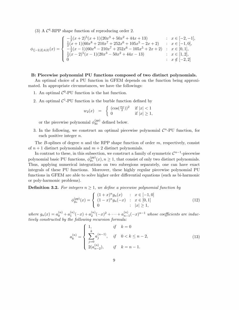
(3) A C4-RPP shape function of reproducing order 2.
φ([−2,2];4;2)(x) =
−12(x+ 2)5(x+ 1)(20x3 + 50x2 + 44x+ 13) : x ∈ [−2,−1],12(x+ 1)(60x8 + 210x7 + 252x6 + 105x5 − 2x+ 2) : x ∈ [−1, 0],−12(x− 1)(60x8 − 210x7 + 252x6 − 105x5 + 2x+ 2) : x ∈ [0, 1],12(x− 2)5(x− 1)(20x3 − 50x2 + 44x− 13) : x ∈ [1, 2],0 : x /∈ [−2, 2]
B: Piecewise polynomial PU functions composed of two distinct polynomials.An optimal choice of a PU function in GFEM depends on the function being approxi-
mated. In appropriate circumstances, we have the followings:
1. An optimal C0-PU function is the hat function.
2. An optimal C1-PU function is the burble function defined by
w2(x) =
(cos(πx2 ))2 if |x| < 1
0 if |x| ≥ 1,
or the piecewise polynomial φ(pp)g2 defined below.
3. In the following, we construct an optimal piecewise polynomial Cn-PU function, foreach positive integer n.
The B-splines of degree n and the RPP shape function of order m, respectively, consistof n+ 1 distinct polynomials and m+ 2 distinct polynomials.
In contrast to these, in this subsection, we construct a family of symmetric Cn−1-piecewisepolynomial basic PU functions, φ
(pp)gn (x), n ≥ 1, that consist of only two distinct polynomials.
Thus, applying numerical integrations on two subregions separately, one can have exactintegrals of these PU functions. Moreover, these highly regular piecewise polynomial PUfunctions in GFEM are able to solve higher order differential equations (such as bi-harmonicor poly-harmonic problems).
Definition 3.2. For integers n ≥ 1, we define a piecewise polynomial function by
φ(pp)gn (x) =
(1 + x)ngn(x) : x ∈ [−1, 0](1− x)ngn(−x) : x ∈ [0, 1]0 : |x| ≥ 1,
(12)
where gn(x) = a(n)0 + a
(n)1 (−x) + a
(n)2 (−x)2+ · · ·+ a
(n)n−1(−x)n−1 whose coefficients are induc-
tively constructed by the following recursion formula:
a(n)k =
1, if k = 0k∑
j=0
a(n−1)j , if 0 < k ≤ n− 2,
2(a(n)n−2), if k = n− 1.
(13)
9
The the coefficients a(n)k can also be obtained by the following recursion formula:
a(n)k =
1 if k = 0,
(n+ k − 1
k)a(n)k−1 if 1 ≤ k ≤ n− 1.
(14)
Let us note the followings:
1. The second recurrence relation implies that a(n)1 = n for each n.
2. Using the recurrence relation (13), gn(x) is as follows:
g1(x) = 1
g2(x) = 1− 2x
g3(x) = 1− 3x+ 6x2,
g4(x) = 1− 4x+ 10x2 − 20x3,
g5(x) = 1− 5x+ 15x2 − 35x3 + 70x4,
g6(x) = 1− 6x+ 21x2 − 56x3 + 126x4 − 252x5,
g7(x) = 1− 7x+ 28x2 − 84x3 + 210x4 − 462x5 + 924x6,
......
...
φ(pp)g1 , φ
(pp)g7 , φ
(pp)g20 , and φ
(pp)g30 that are C0, C6, C19, C29- functions, respectively, are depicted
and compared in Fig. 1.
3. φ(pp)g1 is the hat function which is a C0-piecewise linear PU function. φ
(pp)g2 is a C1-
piecewise cubic polynomial PU function.
By using induction arguments, we prove that the piecewise polynomial functions con-structed above are actually basic PU functions.
Lemma 3.1. For all n ≥ 1, gn(x) satisfies the following relation:
1− xngn(x− 1) = (1− x)ngn(−x). (15)
Proof. For n = 1, 2, 3, one can easily show that the relation (15) holds.By an induction argument, we show that it holds for n + 1 if we assume that it holds
for n. Observing that the coefficients of gn(x) of (13) are written as a0 = a(n−1)0 , a
(n)1 =
a(n−1)0 + a
(n−1)1 , · · · , a(n)n−1 = 2a
(n)n−2.
Now we have
gn(−x) = 1 +n−1∑
k=1
a(n)k xk = xn−1
[
(1
x)n−1 +
n−1∑
k=1
a(n)k (
1
x)n−k−1
]
. (16)
10
Let
(1
x)n−1 +
n−1∑
k=1
a(n)k (
1
x)n−k−1 = (
1
x− 1)
[
(1
x)n−2 +
n−2∑
k=1
bk(1
x)n−k−2
]
+ bn−1.
where, upon using (13),
bk = 1 +k∑
j=1
a(n)j = a
(n+1)k , k = 0, 1, 2, ..., n− 1
Therefore, upon using a(n+1)n = 2a
(n+1)n−1 ,
gn(−x) = (1− x)[
n−2∑
k=0
a(n+1)k xk
]
+ a(n+1)n−1 xn−1
= (1− x)[
gn+1(−x)− a(n+1)n−1 xn−1 − a(n+1)n xn]
+ a(n+1)n−1 xn−1
= (1− x)gn+1(−x)− a(n+1)n xn + a(n+1)n−1 xn + a(n+1)n xn+1
= (1− x)gn+1(−x) + xn(
a(n+1)n x− a(n+1)n−1
)
(17)
Thus
(1− x)ng(−x) = (1− x)n+1gn+1(−x) + (1− x)nxn(
a(n+1)n x− a(n+1)n−1
)
(18)
On the other hand, by replacing x with 1− x in Eqt. (17), we have
1− xngn(x− 1) = 1− xn[
xgn+1(x− 1) + (1− x)n(
a(n+1)n (1− x)− a(n+1)n−1
)
]
= 1− xn+1gn+1(x− 1)− xn(1− x)n[
− a(n+1)n x+ a(n+1)n − a(n+1)n−1
]
= 1− xn+1gn+1(x− 1) + xn(1− x)n[
a(n+1)n x− a(n+1)n−1
]
(19)
Now, by applying induction hypotheses in the right hand sides of (18) and (19), we have theidentity
(1− x)n+1gn+1(−x) = 1− xn+1gn+1(x− 1),
for n+ 1.
Theorem 3.1. For all n ≥ 1, the piecewise polynomial functions φ(pp)gn defined by (12) satisfy
the following.
(i) φ(pp)gn (x) ∈ Cn−1(R),
(ii) φ(pp)gn (x− 1) + φ(pp)gn (x) + φ(pp)gn (x+ 1) = 1 for x ∈ (−1, 1),(iii) The degrees of the polynomial on each subinterval are (2n− 1),
(iv) φ(pp)gn (x) is symmetric about the y-axis,
(v)
∫
R
φ(pp)gn (x)dx = 1.
11
Proof. (i), (iii), and (iv) are straight forward.If x ∈ [0, 1], then applying (15), we have the followings:
∑
k∈Z
φ(pp)gn (x− k) = (1− x)ngn(−x) + xngn(x− 1)
=[
1− xngn(x− 1)]
+ xngn(x− 1) = 1,
which is the proof of (ii).The proof of (v) is as follows:
∫ 0
−1(1 + x)ngn(x)dx =
∫ 1
0(1− x)ngn(−x)dx(by the symmetry property)
=
∫ 1
0
[
1− xngn(x− 1)]
dx(by the relation (15))
Thus,∫ 0
−1(1 + x)ngn(x)dx+
∫ 1
0xngn(x− 1)dx = 1.
By substitution: x− 1 = −t, the second integral becomes
∫ 1
0xngn(x− 1)dx =
∫ 1
0(1− t)ngn(−t)dt.
Thus, we have the property (v).
The converse of Theorem 3.1 is also true. In other words, we have the following uniquenesstheorem:
Theorem 3.2. (Uniqueness) A piecewise polynomial ψ(x) satisfies the following conditions:
1. ψ(x) is symmetric about the y-axis
2. ψ(x) is composed of exactly two polynomials of degree 2n− 1.
3. ψ(x) is a Cn−1-PU function.
4. ψ(0) = 1, and supp(ψ(x)) = [−1, 1].
if and only ifψ(x) = φ(pp)gn .
12

Proof. We only need to prove the necessary part: Let us denote the restriction of ψ(x) onto[0, 1] by ψ+(x). Since ψ(x) is a PU function,
ψ(x+ 1) + ψ(x) + ψ(x− 1) = 1, for x ∈ [−1, 1].
Moreover, ψ(x) ∈ Cn−1(R), we have the following:
djψ(x)
dxj|x=0 = 0, for j = 1, · · · , n− 1,
ψ(x)|x=0 = 1,
ψ+(x) = (1− x)n(b0 + b1x+ b2x2 + · · ·+ bn−1x
n−1).
Consider the difference of two functions:
G(x) = (1− x)ngn(−x)− ψ+(x)= (1− x)n[(a(n)0 − b0) + (a
(n)1 − b1)x+ · · ·+ (a
(n)n−1 − bn−1)xn−1]
Then, we haveG(0) = G′(0) = G′′(0) · · · = G(n−1)(0) = 0,
which implies thatψ+(x) = (1− x)ngn(−x), for all x ∈ [0, 1].
By using the second recursion formula, we can compute the maximum norm of the gradient
of φ(pp)gn for all n.
Theorem 3.3. For the Cn−1-PU function φ(pp)gn (x) = (1 + x)ngn(x) defined by (12), we have
the following:
(i) ‖[φ(pp)gn ]′‖∞ = (2n− 1)a(n)n−1(
14)n−1.
(ii) φ(pp)gn (x) is monotonically increasing on [−1, 0].
(iii) ‖[φ(pp)gn ]′′‖∞ = (2n− 1)(n− 1)a(n)n−1|Q(1 +Q)|n−2|2Q+ 1|, where
Q =[
(4n− 6) +√
2(4n− 6)]
/2(4n− 6).
Proof. From the definition 3.2, we have
[φ(pp)gn ]′(x) = n(1 + x)n−1gn(x) + (1 + x)ng′n(x)
= (1 + x)n−1(
ngn(x) + (1 + x)g′n(x))
.
13

Table 1: The selected maximum values of |[φ(pp)gn ]′(x)| and |[φ(pp)gn ]′′(x)|.
n = 2 n = 3 n = 5 n = 7 n = 10 n = 15 n = 20 n = 30
‖[φ(pp)gn ]′‖∞ 1.5 1.875 2.46 2.93 3.52 4.33 5.01 6.15
‖[φ(pp)gn ]′′‖∞ 5.77 9.37 13.18 18.94 28.97 38.26 57.61
Using (14), we have gn(x) =∑n−1
k=0(−1)ka(n)k xk, a
(n)0 = 1, a
(n)k = n+k−1
k a(n)k−1, 1 ≤
k ≤ n− 1. Hence, we obtain the following relation
ngn(x) + (1 + x)g′n(x)
= n(
1 +n−1∑
k=1
(−1)ka(n)k xk)
+n−1∑
k=1
(−1)kka(n)k xk−1 +n−1∑
k=1
(−1)kka(n)k xk
= n+n−1∑
k=1
(−1)kna(n)k xk +n−2∑
k=0
(−1)k+1(k + 1)a(n)k+1x
k +n−1∑
k=1
(−1)kka(n)k xk
= n− a(n)1 +
n−2∑
k=1
[
(n+ k)a(n)k − (k + 1)a
(n)k+1
]
(−x)k + (2n− 1)a(n)n−1(−x)n−1
= (2n− 1)a(n)n−1(−x)n−1, (20)
which implies |[φ(pp)gn ]′(x)| = (2n−1)a(n)n−1|[−x(1+x)]n−1| whose maximum value occurs when
x = −1/2. Thus we have proved that (i) holds.
Since (1 + x)(n−1) ≥ 0 for x ∈ [−1, 0], (20) implies that [φ(pp)gn ]′(x) ≥ 0, x ∈ [−1, 0]; and
hence the assertion (ii) follows.Applying (20), we have a simple form of the second order derivative
[φ(pp)gn ]′′(x) = −(2n− 1)(n− 1)a(n)n−1[−x(1 + x)]n−2(2x+ 1), (21)
and hence the maximum of the second order derivative occurs when x = [(4n − 6) +√
2(4n− 6)]/2(4n− 6).
In table 1 and Fig. 1, the maximum vales of the first derivative and the second orderderivative of piecewise polynomial PU functions are shown. These maximum values are partsof error bounds for GFEM in Theorem 4.1.
C: The convolution PU shape functionsThus far, we have introduced four different kinds of PU shape functions associated mainly
with uniformly distributed particles (the Shepard PU functions can be used for non-uniformlypartitioned patches).
14

X
Y
-1 -0.5 0 0.5 10
0.2
0.4
0.6
0.8
1
1.2phi_g1phi_g7phi_g20phi_g30
N
MA
XIM
UM
NO
RM
0 5 10 15 20 25 300
1
2
3
4
5
6
7
1ST DER(2ND DER)/10
Figure 1: [Left:] The piecewise polynomial PU functions φ(pp)g1 , φ
(pp)g7 , φ
(pp)g20 , φ
(pp)g30 that are
C0-, C6-, C19-, C29- functions, respectively. [Right:] ‖[φ(pp)gn ]′‖∞, for n = 1, ..., 30 and
‖[φ(pp)gn ]′′‖∞/10, for n = 3, ..., 30
Now we construct a family of functions that is a partition of unity subordinate to anarbitrary covering of a given domain. These PU functions are also used to deal with uniformly(or non uniformly) distributed particles in Meshfree particle methods ([18]).
Consider the scaled window function defined by
w(l)δ (x) = Aw(
x
δ), (22)
where w(x) = (1− x2)l, |x| ≤ 1, is the conical window function defined by (1) and
A−1 =
∫ δ
−δw(x
δ)dx.
Let Qk = (xk, xk+1) be an interval with |xk+1 − xk| ≥ 2δ and the characteristic functionof Qk is defined by
χQk(x) =
1, if x ∈ Qk,0, if x /∈ Qk.
(23)
15
Definition 3.3. The convolution PU function of χQkand w
(l)δ is defined by
ψ(δ,l)k (x) =
∫
R
w(l)δ (x− y)χQk
(y)dy =
∫
Qk
w(l)δ (x− y)dy
=
fk+1(x) =
∫ δ
x−xk+1
w(l)δ (t)dt, if x ∈ [xk+1 − δ, xk+1 + δ],
1, if x ∈ [xk + δ, xk+1 − δ],
fk(x) =
∫ x−xk
−δw(l)δ (t)dt, if x ∈ [xk − δ, xk + δ],
0, if x ∈ R\[xk − δ, xk+1 + δ].
(24)
Since the scaled window function is a polynomial, ψ(δ,l)k (x) becomes a piecewise polyno-
mial.Next, we show that for a fixed δ and a fixed l, ψ(δ,l)k becomes a partition of unity.
Suppose a domain Ω = (a, b) is uniformly (or non-uniformly) partitioned as follows:
x1 = a− δ < a < x2 < · · ·xk < xk+1 · · · < xn < b < xn+1 = b+ δ
so thatxk+1 − xk ≥ 2δ, for 1 ≤ k ≤ n.
Let Qk = (xk, xk+1), k = 1, · · · , n. Then we have
n∑
k=1
χQk(x) = 1, for all x ∈ Ω, except the nodal points, (25)
which implies
n∑
k=1
ψ(δ,l)k (x) =
n∑
k=1
[∫
R
χQk(x− y))wδ(y)dy
]
= 1, for all x ∈ Ω. (26)
Thus, these piecewise polynomial ψ(δ,l)k have the following properties:
Theorem 3.4. 1. supp(ψ(δ,l)k (x)) = [xk − δ, xk+1 + δ].
2. ψ(δ,l)k (x) : k = 1, · · · , n is a partition of unity subordinate to an arbitrary coveringQδ
k = (xk − δ, xk+1 + δ) : k = 1, · · · , n of Ω such that any two are overlapped on aninterval with 2δ length.
3.
(a) ψ(δ,l)k (x) ∈ Cl(R), (27)
(b) max | ddx
(ψ(δ,l)k (x))| = max |w(l)δ | = A = O(δ−1). (28)
16
Proof. (1), (2), and (3-b) are obvious. We only need to prove (3-a).
dψ(δ,l)k (x)
dx=
−w(l)δ (x− xk+1) if x ∈ [xk+1 − δ, xk+1 + δ],0, if x ∈ [xk + δ, xk+1 − δ],w(l)δ (x− xk) if x ∈ [xk − δ, xk + δ],
0, if x ∈ R\[xk − δ, xk+1 + δ].
(29)
which is continuous and (l − 1) differentiable. Thus, the convolution PU function is a C l-function.
For example, we have the specific expressions as follows:
• If l = 3 in the conical window function (1), then the polynomials fk(x) and fk+1(x) areas follows:
fk+1(x) = (1
32δ7)
[16δ3 + 29δ2(x− xk+1) + 20δ(x− xk+1)2 + 5(x− xk+1)3]
(δ − x+ xk+1)4
(30)
fk(x) = (1
32δ7)
[16δ3 − 29δ2(x− xk) + 20δ(x− xk)2 − 5(x− xk)3]
(δ + x− xk)4
. (31)
• If l = 5 in the conical window function, then
max | ddx
(ψ(δ,l)k (x))| < (1.28)× 10p, if δ = 10−p, p = 0, 1, 2, . . . .
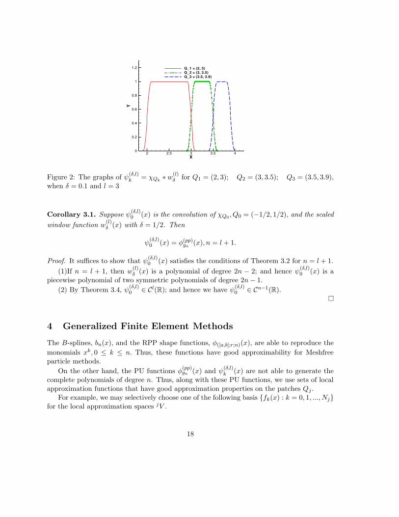
• For δ = 0.1, l = 3, the PU functions, ψ(δ,l)k (x), are depicted in Fig. 2 whenQk, k = 1, 2, 3,
respectively, are (2, 3), (3, 3.5) and (3.5, 3.9).
As a special case of this convolution PU function, by taking
δ = 1/2, xk = −1/2, xk+1 = 1/2
in (30) and (31), we obtain the following C3-piecewise polynomial PU function consisting ofexactly two distinct polynomials:
ψ(1/2,3)[−1,1] =
(1 + x)4(1− 4x+ 10x2 − 20x3) : x ∈ [−1, 0],(1− x)4(1 + 4x+ 10x2 + 20x3) : x ∈ [0, 1],0 : |x| ≥ 1.
Hence, we have reproduced φ(pp)g4 as a special case of the convolution PU functions.
Generally, we have the following:
17
X
Y
2 2.5 3 3.5 40
0.2
0.4
0.6
0.8
1
1.2 Q_1 = (2, 3)Q_2 = (3, 3.5)Q_3 = (3.5, 3.9)
Figure 2: The graphs of ψ(δ,l)k = χQk
∗ w(l)δ for Q1 = (2, 3); Q2 = (3, 3.5); Q3 = (3.5, 3.9),when δ = 0.1 and l = 3
Corollary 3.1. Suppose ψ(δ,l)0 (x) is the convolution of χQ0
, Q0 = (−1/2, 1/2), and the scaled
window function w(l)δ (x) with δ = 1/2. Then
ψ(δ,l)0 (x) = φ(pp)gn (x), n = l + 1.
Proof. It suffices to show that ψ(δ,l)0 (x) satisfies the conditions of Theorem 3.2 for n = l + 1.
(1)If n = l + 1, then w(l)δ (x) is a polynomial of degree 2n − 2; and hence ψ
(δ,l)0 (x) is a
piecewise polynomial of two symmetric polynomials of degree 2n− 1.
(2) By Theorem 3.4, ψ(δ,l)0 ∈ Cl(R); and hence we have ψ
(δ,l)0 ∈ Cn−1(R).
4 Generalized Finite Element Methods
The B-splines, bn(x), and the RPP shape functions, φ([a,b];r;n)(x), are able to reproduce the
monomials xk, 0 ≤ k ≤ n. Thus, these functions have good approximability for Meshfreeparticle methods.
On the other hand, the PU functions φ(pp)gn (x) and ψ
(δ,l)k (x) are not able to generate the
complete polynomials of degree n. Thus, along with these PU functions, we use sets of localapproximation functions that have good approximation properties on the patches Qj .
For example, we may selectively choose one of the following basis fk(x) : k = 0, 1, ..., Njfor the local approximation spaces jV .
18
(1)fk(ξ) = ξk : k = 0, 1, ..., Nj , which are monomials.
(2)fk(ξ) = L(0)k (ξ) : k = 0, 1, ..., Nj , which are orthogonal polynomials with respect to the
weight(
φ(pp)gn
)2on [−1, 1].
(3)fk(ξ) = L(1)k (ξ) : k = 0, 1, ..., Nj , which are orthogonal polynomials with respect to the
weight(
[φ(pp)gn ]′
)2on [−1, 1].
(4) Let −1 = ξ0, ξ1, · · · , ξNj= 1 be (Nj + 1) distinct points in [−1, 1] and consider the
Lagrange interpolating polynomials:
LNj ,k(ξ) =
Nj∏
i=0,i6=k
(ξ − ξi)(ξk − ξi)
, k = 0, 1, · · · , Nj
Then, for any polynomial p(x) of degree ≤ Nj , we have
Nj∑
k=0
p(xk)LNj ,k(x) = p(x), for all x ∈ R.
That is, LNj ,k(x) : k = 0, 1, · · · , Nj reproduces the polynomials of degree ≤ Nj .
In this paper, we view LNj ,k(x) as a global polynomial defined on R.
(5) fk(ξ) = sin k(π/2)(ξ + 1) : k = 0, 1, ..., Nj , which are the sine functions with variousfrequencies.
The special orthogonal polynomials, L(0)k (ξ) and L
(1)k (ξ), for the local approximation func-
tions, are constructed in the appendix.
4.1 GFEM for uniformly distributed patches
Let
Ω = (a, b),
h = (b− a)/N,Qhj = (a+ h(j − 1), a+ h(j + 1)), j = 1, 2, · · · , N.
Next, we define a linear patch mapping Ψj : [−1, 1] −→ Qhj as follows:
Ψj(ξ) = hξ + xj , (32)
where xj = a+ hj, j = 0, · · · , n. Let
ψ(pp)j (x) = (φ(pp)gn Ψ
−1j )(x).
19
Then ψ(pp)j (x) : j = 0, 1, · · · , N is a partition of unity subordinate to the covering Qhj :
j = 0, 1, 2, · · · , N of Ω. Note that some patches Qhj may go outside Ω.
Now, for each j, let
jV = span[
jϕk(x) := fk Ψ−1j (x)]
; k = 0, 1, ..., Nj
be a local approximation space on Qhj , where fk : k = 0, 1, ..., Nj is a basis of the local
approximation space on the patch Qhj .
Then a GFEM approximation space is defined by
Vh = span[ψ(pp)j · jϕk] : k = 0, 1, 2, ..., Nj , j = 0, 1, ..., N. (33)
Now the Galerkin approximation method associated with the finite dimensional vector space
Vh is as follow: Find uh =∑N
j=0
∑Nj
k=0 cjk[ψ(pp)j (x) · jϕk(x)] such that
B1(uh, ψ(pp)i (x) · iϕk(x)) = F1(ψ(pp)i (x) · iϕk(x)) for (3), (34)
B2(uh, ψ(pp)i (x) · iϕk(x)) = F2(ψ(pp)i (x) · iϕk(x)) for (6), (35)
for all i and k.This method is said to be generalized finite element method (GFEM).
Remark 4.1. (1) Unlike the shepard-type PU functions, ψ(pp)j and its derivatives are piece-
wise polynomials consisting of only two distinct polynomials (the minimal number for piece-wise polynomials). Thus, the numerical integrals, in the bilinear forms of (34) and (35),are exact by computing the integrals on two subintervals whenever the local approximationfunctions are polynomials.
(2) The advantage of GFEM is the freedom of selectively choosing local approximationfunctions. If the function to be approximated contains a singularity on a patch Qh
j , then onecan chose singular local approximation functions that resembles the singularity. In this case,the numerical integral can not be exact. Optimal choices of local approximation spaces areextensively discussed in ([5]).
(3) Using these orthogonal polynomial approximation functions has some advantages overusing the monomial approximation functions in computing stiffness matrices. However, it hasdisadvantages in dealing with essential boundary conditions as it is shown in the numericalexamples of section 5.
[Numerical Integrations for Second Order Equations]In the following, we will suppress h in Qh
j , and will write it by by Qj .
20
Typical components of the stiffness matrix of the system (34) are of the form
(1)
∫
Qi
[ψ(pp)i · iϕk]′ · [ψ
(pp)i · iϕl]′dx
=
∫
Qi
(
[ψ(pp)i ]′ · iϕk + ψ
(pp)i · [iϕk]′
)(
[ψ(pp)i ]′ · iϕl + ψ
(pp)i · [iϕl]′
)
dx, (36)
(2)
∫
Qi∩Qj
[ψ(pp)i · iϕk]′ · [ψ
(pp)j · jϕl]′dx
=
∫
Qi∩Qj
(
[ψ(pp)i ]′ · iϕk + ψ
(pp)i · [iϕk]′
)(
[ψ(pp)j ]′ · jϕl + ψ
(pp)j · [jϕl]′
)
dx, (37)
where j is either i− 1 or i+ 1.The components of the load vector are of the form
∫
Qi
f(x)[·ψ(pp)i (x) · iϕk(x)]dx. (38)
Now these integrals can be transformed into integrals on the reference patch Q = [−1, 1]by the patch mapping Ψi. For example, the details of computing these components are asfollows:
∫
Qi∩Qi−1
d
dx(ψ(pp)i · iϕk) ·
d
dx(ψ(pp)i−1 · i−1ϕl)dx
=
∫ 0
−1h
[
d
dx([φ(pp)gn · fk] Ψ
−1i )
]
Ψi ·[
d
dx([φ(pp)gn · fl] Ψ
−1i−1)
]
Ψi · dξ
=
∫ 1
−1
1
2h
[
d
dξ(φ(pp)gn · fk)
]
(ξ − 1
2) ·[
d
dξ(φ(pp)gn · fl)
]
(ξ + 1
2) · dξ
On the other hand, if we expand (36) and consider termwise integrations, then each termof these integrals can be expressed as
∫ 1
−1G(ξ) · d
l[φ(pp)gn ]
dξl(ξ) · d
m[φ(pp)gn ]
dξm(ξ) · pk(ξ)dξ, 0 ≤ l,m ≤ 1
=
∫ 0
−1G(ξ) · d
l[φ(pp)gn ]
dξl(ξ) · d
m[φ(pp)gn ]
dξm(ξ) · pk(ξ)dξ
+
∫ 1
0G(ξ) · d
l[φ(pp)gn ]
dξl(ξ) · d
m[φ(pp)gn ]
dξm(ξ) · pk(ξ)dξ (39)
where G(ξ) is the product of Jacobian functions and the coefficient functions of differentialequation, and pk(ξ) is a product of two local approximation functions or their derivatives.Hence, pk(ξ) is a polynomial when the local approximation functions are polynomials.
Thus, we have the following features about the numerical integrations for the stiffnessmatrices:
21
• IfG(ξ) is a polynomial and local approximation functions are polynomial, the integrandsof the last two integrals are polynomials, and hence one can exactly calculate stiffnessmatrices at a lower computing cost.
• Or, we can observe the computation of stiffness matrices as numerical integrations ofthe form
∫ 1
−1W
ord(2)1 (ξ)g(ξ)dξ, (40)
where g(ξ) = G(ξ) · pk(ξ) and W ord(2)1 (ξ) is one of the following functions:
φ(ξ), φ(ξ)φ(ξ), φ(ξ)φ′(ξ), φ′(ξ)φ′(ξ), (41)
where φ(ξ) = [φ(pp)gn ](ξ).
Along this interpretation, we have to deal with numerical integrations of the form
∫ 1
0W
ord(2)2 (ξ)g(ξ)dξ, (42)
where Word(2)2 (ξ) is one of the tensor product φ((ξ +1)/2), φ′((ξ +1)/2)⊗ 1, φ((ξ −
1)/2), φ′((ξ − 1)/2). More specifically, it is one of the following functions:
φ((ξ + 1)/2) φ((ξ − 1)/2)φ((ξ + 1)/2) φ′((ξ − 1)/2)φ(ξ + 1)/2)φ((ξ − 1)/2)φ′(ξ + 1)/2) φ′((ξ − 1)/2)φ′(ξ + 1)/2)
(43)
For effective calculations of these integrals, we could consider eight quadrature ruleswith respect to these eight weight functions listed in (41) and (43). However, we some-times use singular local approximation functions on a patch containing singularity. Inthis case, we have no advantages in using these special quadrature rules. However, onecan selectively use these special quadrature rules for the patches where local approx-imation functions are polynomials. The orthogonal polynomials to weight functions
W (x) = [φ(pp)gn ]2 and W (x) = [ ddxφ
(pp)gn ]2 are given in appendix.
[Numerical Integrations for Fourth Order Equations]Typical components of the stiffness matrix of the system (35) are of the form
(1)
∫
Qi
(
[ψ(pp)i ]′′ · iϕk + 2[ψ
(pp)i ]′ · iϕ′k + [ψ
(pp)i ] · iϕ′′k
)
·(
[ψ(pp)i ]′′ · iϕl + 2[ψ
(pp)i ]′ · iϕ′l + [ψ
(pp)i ] · iϕ′′l
)
dx, (44)
(2)
∫
Qi∩Qj
(
[ψ(pp)i ]′′ · iϕk + 2[ψ
(pp)i ]′ · iϕ′k + [ψ
(pp)i ] · iϕ′′k
)
·(
[ψ(pp)j ]′′ · jϕl + 2[ψ
(pp)j ]′ · jϕ′l + [ψ
(pp)j ] · jϕ′′l
)
dx, (45)
22

where j = i+ 1, i− 1, and components of the load vector are of the form
∫
Qi
f(x) · [ψ(pp)i ](x) · iϕk(x)dx. (46)
Similarly, letting [ψ(pp)j ] = φ, we have the following relation for the fourth order equations:
∫
Qi∩Qi−1
d2
dx2([ψ
(pp)i ] · iϕk) ·
d2
dx2([ψ
(pp)i−1 ] · i−1ϕl)dx
=
∫ 0
−1h
[
d2
dx2([φ · fk] Ψ−1i )
]
Ψi ·[
d2
dx2([φ · fl] Ψ−1i−1)
]
Ψi · dξ
=
∫ 1
−1
1
2h3
[
d2
dξ2(φ · fk)
]
(ξ − 1
2) ·[
d2
dξ2(φ · fl)
]
(ξ + 1
2) · dξ
The integrand of the last integral is a polynomial on [−1, 0] and on [0, 1] whenever the localapproximation functions are polynomials. Hence, the components of the stiffness matricescan be exactly computed in such cases.
4.2 Error bounds
In this section, by using existing error analysis ([2]), we state more specific error bounds of
GFEM with respect to the piecewise polynomial PU function φ(pp)gn .
Let (Ψ(pp)n )i(x) = φ
(pp)gn ((x−xi)/h). Then from Table 1, we have specific error bounds: for
example, if n = 3, then
‖(Ψ(pp)n )i(x)‖L∞(R) = 1, (47)
‖ ddx
(Ψ(pp)n )i(x)‖L∞(R) = ‖[φ(pp)gn ]′‖L∞(R)/h < 1.88/h, (48)
‖ d2
dx2(Ψ(pp)n )i(x)‖L∞(R) =
[
‖[φ(pp)gn ]′′‖L∞(R)]
/h2 < 5.77/h2. (49)
Thus, Theorem 6.1 of [2] can be modified as follows:
Theorem 4.1. Suppose u ∈ H2(Ω) and φ(pp)gn is a basic PU function in GFEM. If, for all
i = 0, 1, 2, ..., N, there exists iu(gfe) on each patch Qi such that
‖u− iu(gfe)‖L2(Ω∩Qi) ≤ ε1(i), (50)
‖ ddx
(u− iu(gfe))‖L2(Ω∩Qi) ≤ ε2(i), (51)
‖ d2
dx2(u− iu(gfe))‖L2(Ω∩Qi) ≤ ε3(i). (52)
23

Then, the GFE solution
u(gfe) =N∑
i=0
Ψ(pp)i · iu(gfe) ∈ Vh
satisfies
‖u− u(gfe)‖L2(Ω) ≤√2
(
N∑
i=0
ε1(i)2
)1/2
(53)
‖ ddx
(u− u(gfe))‖L2(Ω) ≤ 2
(
N∑
i=0
[
ε2(i)2 + (‖[φ(pp)gn ]′‖L∞(R)/h)2ε1(i)2
]
)1/2
(54)
‖ d2
dx2(u− u(gfe))‖L2(Ω) ≤ 2
(
N∑
i=0
[
ε3(i)2 + 2(‖[φ(pp)gn ]′‖L∞(R)/h)2ε2(i)2
+(
[‖[φ(pp)gn ]′′‖L∞(R)/h2]ε1(i))2])1/2
(55)
Proof. The proofs of (53) and (54) are similar to the proofs of Theorem 6.1 of [2]. Thus, weonly need to prove (55) that is not in [2].
Since Ψ(pp)i : i = 0, 1, ..., N is a partition of unity subordinate to the open coveringQi : i = 0, 1, 2, ..., N,
‖ d2
dx2(u− u(gfe))‖2L2(Ω)
= ‖ d2
dx2
N∑
i=0
Ψ(pp)i (u− iu(gfe))‖2L2(Ω)
≤ 2‖N∑
i=0
[ d2
dx2Ψ(pp)i
]
(u− iu(gfe))‖2L2(Ω)+ 4‖
N∑
i=0
d
dxΨ(pp)i
d
dx(u− iu(gfe))‖2L2(Ω)
+ 2‖N∑
i=0
Ψ(pp)i
[ d2
dx2(u− iu(gfe))
]
‖2L2(Ω). (56)
For each x ∈ Ω ⊂ R, the sums of (56) have at most two nonzero terms. Therefore, we have
|N∑
i=0
[ d2
dx2Ψ(pp)i
][
(u− iu(gfe))]
|2 ≤ 2
N∑
i=0
|[ d2
dx2Ψ(pp)i
][
(u− iu(gfe))]
|2,
|N∑
i=0
[ d
dxΨ(pp)i
][ d
dx(u− iu(gfe))
]
|2 ≤ 2N∑
i=0
|[ d
dxΨ(pp)i
][ d
dx(u− iu(gfe))
]
|2,
|N∑
i=0
[
Ψ(pp)i
][ d2
dx2(u− iu(gfe))
]
|2 ≤ 2N∑
i=0
|[
Ψ(pp)i
][ d2
dx2(u− iu(gfe))
]
|2 .
Hence, (47), (48), (49), and (56) imply the desired result.
24

5 Numerical solutions of the second and the fourth order el-
liptic equations
In this section, we solve the second order and the fourth order differential equations by using
the GFEM approximation space constructed with aid of the PU functions φ(pp)gn .
Let us note that for the numerical solutions for the second order equations, we can employ
the PU functions φ(pp)gn for all n ≥ 1. However, for the fourth order equations, we use the PU
function φ(pp)gn for n ≥ 3 in GFEM.
Let U(w) = 1
2B(w,w) be the strain energy of w, where B(·, ·) denote the bilinear forms
defined in section 2. Then the relative error in energy norm is defined as
‖e‖E,r =[ |U(uex)− U(uapp)|
U(uex)
]1/2
.
All test problems of this section are solved by GFEM with respect to following data
Ω = (−1, 1),h = 0.5,
xi = −1 + h · i, i = 0, 1, 2, ..., 4,
Ni = M, for all i (uniform dimension of local approximation spaces).
5.1 Numerical Solutions for the Second Order Differential Equations
Example 1. u(x) = ex(1− x2) solves the following model problem
− d2
dx2u(x) = f(x) in (−1, 1),
where f(x) = ex(1 + 4x+ x2). Then the strain energy is
1
2
∫
Ω(du
dx)2dx = 2.6524776642670.
To compare an approximablity of local approximation functions: φ(pp)gn (ξ) ⊗ fk(ξ) : k =
0, 1, 2, · · · , N, we test a various piecewise polynomial PU functions, φ(pp)g1 (the hat function),
φ(pp)g3 , φ
(pp)g7 , and φ
(pp)g30 in GFEM.
As one can see from Table 2 and Fig. 3, GFEM for all of these piecewise polynomial PUfunctions yields highly accurate results. Theorem 4.1, together with Theorem 3.3(or Table
1), implies that the errors are getting bigger as n (in φ(pp)gn ) is increasing. Results in Table 2
and Fig. 3 support this theory.
25

Table 2: Relative error (%) in energy norm (‖e‖E,r × 100) of GFEM solutions when the
piecewise polynomial PU functions φ(pp)gn , n = 1, 3, 7, 30, respectively, are used
p-deg g1 g3 g7 g301 6.703986 25.2157 29.8296 32.1909
2 0.505911 2.83537 0.8166 2.18725
3 0.024968 0.20079 0.0908 0.22226
4 0.000834 0.00910 0.0080 0.00620
5 0.000335 0.00076 0.0017 0.00434
6 0.000058 0.00087 0.0016 0.00433
P-Degree
RE
LA
TIV
EE
RR
OR
(%)
INE
NE
RG
YN
OR
M
1 2 3 4 5 6 710-5 10-5
10-4 10-4
10-3 10-3
10-2 10-2
10-1 10-1
100 100
101 101
g1g3g7g30
P-Degree
RE
LA
TIV
EE
RR
OR
(%)
INE
NE
RG
YN
OR
M
1 2 3 4 5 6 7 8 9
10-4 10-4
10-3 10-3
10-2 10-2
10-1 10-1
100 100
101 101
Orthognal BaseMonomial Base
P-Degree
RE
LA
TIV
EE
RR
OR
(%)
INE
NE
RG
YN
OR
M
1 2 3 4 5 6 7 8 9
10-4 10-4
10-3 10-3
10-2 10-2
10-1 10-1
100 100
101 101
Orthognal BaseMonomial Base
P-Degree
RE
LA
TIV
EE
RR
OR
(%)
INE
NE
RG
YN
OR
M
1 2 3 4 5 6 7 8 9
10-4 10-4
10-3 10-3
10-2 10-2
10-1 10-1
100 100
101 101
Orthognal BaseMonomial Base
P-Degree
RE
LA
TIV
EE
RR
OR
(%)
INE
NE
RG
YN
OR
M
1 2 3 4 5 6 7 8 9
10-4 10-4
10-3 10-3
10-2 10-2
10-1 10-1
100 100
101 101
Orthognal BaseMonomial Base
Figure 3: [Left] Relative error(%) in energy norm of GFEM when the piecewise polynomial
PU functions φ(pp)gn , n = 1, 3, 7, 30, respectively, are used. [Right] Relative error (in percent)
in Energy Norm of GFEM solutions for the monomial local approximation functions andthe orthogonal local approximation functions that are orthogonal with respect to the weight
function [φ(pp)g3 ]′(x)2
26
Let Lk(x), k = 0, 1, 2, ... be the sequence of orthogonal polynomials such as Legendrepolynomials and those polynomial in Table 5, and Pk(x) = xk, k = 0, 1, 2, ... be a sequenceof monomials Then
Lk(0) = 0 if k is an odd integerLk(0) 6= 0 if k is an even integer,
and
Pk(0) = 0 if k 6= 0Pk(0) = 1 if k = 0.
Suppose the boundary condition at one end point is Dirichlet and the reference basis functionsare Pk(x) = xk, k = 0, 1, 2, ....,M. Then we only need to constrain P0. On the other hand,if Lk(x), k = 0, 1, 2, ...,M is used as local basis functions, we have to constrain all evendegree orthogonal polynomials L2k(x), k = 0, 1, 2, · · · . In this case, GFEM for the orthogonalbasis functions will lose exactly one half local degree of freedom at the end point node. ThusGFEM for the orthogonal basis functions Lk(x), k = 0, 1, 2, ...,M may yield inferior resultsthan GFEM for the monomial basis functions xk, k = 0, 1, ...,M. This is demonstrated inthe next example.
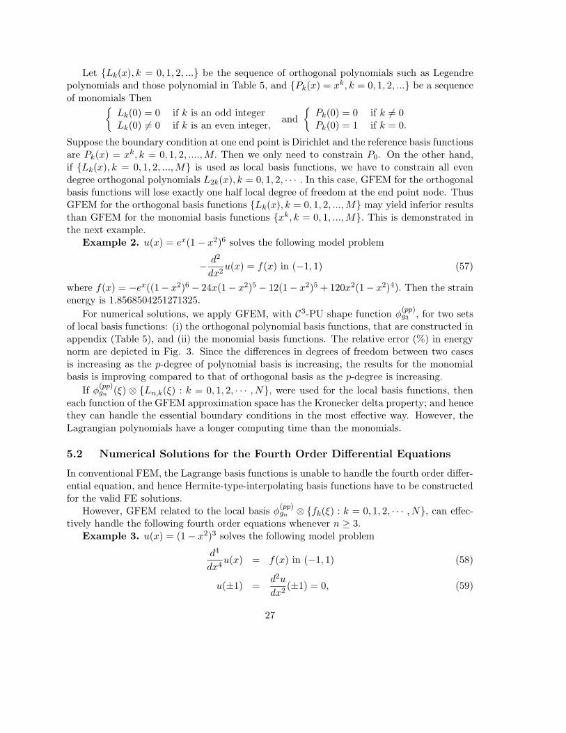
Example 2. u(x) = ex(1− x2)6 solves the following model problem
− d2
dx2u(x) = f(x) in (−1, 1) (57)
where f(x) = −ex((1− x2)6 − 24x(1− x2)5 − 12(1− x2)5 + 120x2(1− x2)4). Then the strainenergy is 1.8568504251271325.
For numerical solutions, we apply GFEM, with C3-PU shape function φ(pp)g3 , for two sets
of local basis functions: (i) the orthogonal polynomial basis functions, that are constructed inappendix (Table 5), and (ii) the monomial basis functions. The relative error (%) in energynorm are depicted in Fig. 3. Since the differences in degrees of freedom between two casesis increasing as the p-degree of polynomial basis is increasing, the results for the monomialbasis is improving compared to that of orthogonal basis as the p-degree is increasing.
If φ(pp)gn (ξ) ⊗ Ln,k(ξ) : k = 0, 1, 2, · · · , N, were used for the local basis functions, then
each function of the GFEM approximation space has the Kronecker delta property; and hencethey can handle the essential boundary conditions in the most effective way. However, theLagrangian polynomials have a longer computing time than the monomials.
5.2 Numerical Solutions for the Fourth Order Differential Equations
In conventional FEM, the Lagrange basis functions is unable to handle the fourth order differ-ential equation, and hence Hermite-type-interpolating basis functions have to be constructedfor the valid FE solutions.
However, GFEM related to the local basis φ(pp)gn ⊗ fk(ξ) : k = 0, 1, 2, · · · , N, can effec-
tively handle the following fourth order equations whenever n ≥ 3.Example 3. u(x) = (1− x2)3 solves the following model problem
d4
dx4u(x) = f(x) in (−1, 1) (58)
u(±1) =d2u
dx2(±1) = 0, (59)
27

Table 3: In case the true solution of the fourth order equation is u(x) = (1 − x2)3, thecomputed Strain Energy and Relative error in percent with respect to the PU function
φ(pp)gn , n = 3, 7, respectively, are presented
φ(pp)g3 φ
(pp)g7
p-deg Strain Energy ‖e‖E,r × 100 Strain Energy ‖e‖E,r × 100
1 7.0006138392856 72.21 3.9575930714358 85.41
2 13.065142760779 32.69 13.422758749197 28.71
3 14.401452691593 12.46 14.584210106868 5.51
4 14.621316438602 2.23 14.627138618156 0.99
5 14.628525836503 0.18 14.628506376614 0.21
6 14.628571428571 0.0 14.628571428571 0.0
7 14.628571428571 0.0 14.628571428571 0.0
where
f(x) = 72− 360x2.
Then the strain energy is
1
2
∫
Ω(d2u
dx2)2dx = 14.6285714285714.
Since the true solution is a polynomial of degree 6, we expect that GFEM with monomiallocal basis yields an exact solution if the p-degree of the polynomial local approximationfunctions is ≥ 6. Table 3 shows the expected results.
Example 4. u(x) = ex(1− x2)6 solves the following model problem
d4
dx4u(x) = f(x) in (−1, 1) (60)
u(±1) =d2u
dx2(±1) = 0, (61)
where
f(x) = ex[
(1− x2)6 − 48(1− x2)5x+ 720(1− x2)4x2 − 72(1− x2)5 − 3840(1− x2)3x3
+ 1440(1− x2)4x+ 5760(1− x2)2x4 − 5760(1− x2)3x2 + 360(1− x2)4]
.
Then the strain energy is
1
2
∫
Ω(d2u
dx2)2dx = 36.5967697946804.
28
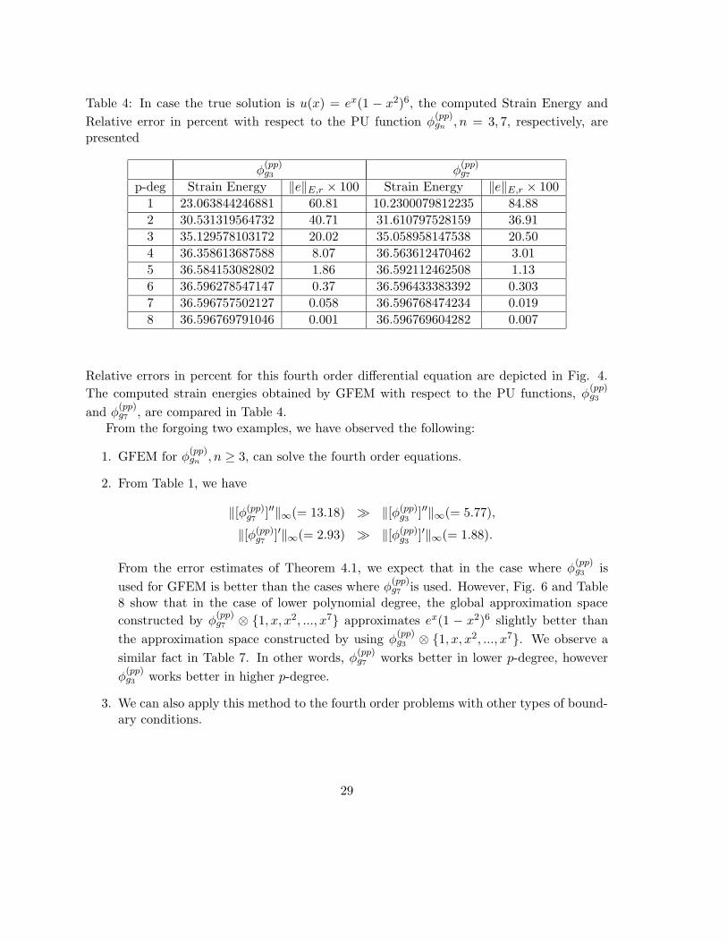
Table 4: In case the true solution is u(x) = ex(1 − x2)6, the computed Strain Energy and
Relative error in percent with respect to the PU function φ(pp)gn , n = 3, 7, respectively, are
presented
φ(pp)g3 φ
(pp)g7
p-deg Strain Energy ‖e‖E,r × 100 Strain Energy ‖e‖E,r × 100
1 23.063844246881 60.81 10.2300079812235 84.88
2 30.531319564732 40.71 31.610797528159 36.91
3 35.129578103172 20.02 35.058958147538 20.50
4 36.358613687588 8.07 36.563612470462 3.01
5 36.584153082802 1.86 36.592112462508 1.13
6 36.596278547147 0.37 36.596433383392 0.303
7 36.596757502127 0.058 36.596768474234 0.019
8 36.596769791046 0.001 36.596769604282 0.007
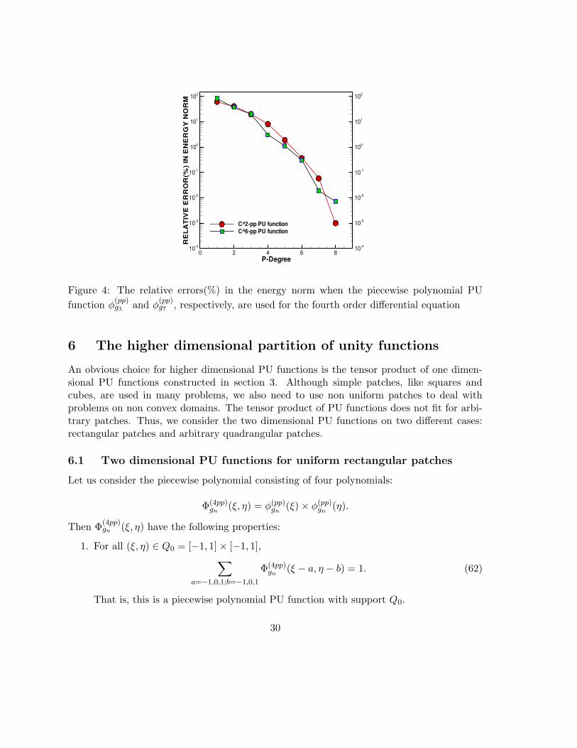
Relative errors in percent for this fourth order differential equation are depicted in Fig. 4.
The computed strain energies obtained by GFEM with respect to the PU functions, φ(pp)g3
and φ(pp)g7 , are compared in Table 4.
From the forgoing two examples, we have observed the following:
1. GFEM for φ(pp)gn , n ≥ 3, can solve the fourth order equations.
2. From Table 1, we have
‖[φ(pp)g7 ]′′‖∞(= 13.18) À ‖[φ(pp)g3 ]′′‖∞(= 5.77),
‖[φ(pp)g7 ]′‖∞(= 2.93) À ‖[φ(pp)g3 ]′‖∞(= 1.88).
From the error estimates of Theorem 4.1, we expect that in the case where φ(pp)g3 is
used for GFEM is better than the cases where φ(pp)g7 is used. However, Fig. 6 and Table
8 show that in the case of lower polynomial degree, the global approximation space
constructed by φ(pp)g7 ⊗ 1, x, x2, ..., x7 approximates ex(1 − x2)6 slightly better than
the approximation space constructed by using φ(pp)g3 ⊗ 1, x, x2, ..., x7. We observe a
similar fact in Table 7. In other words, φ(pp)g7 works better in lower p-degree, however
φ(pp)g3 works better in higher p-degree.
3. We can also apply this method to the fourth order problems with other types of bound-ary conditions.
29
P-Degree
RE
LA
TIV
EE
RR
OR
(%)
INE
NE
RG
YN
OR
M
0 2 4 6 810-4 10-4
10-3 10-3
10-2 10-2
10-1 10-1
100 100
101 101
102 102
C^2-pp PU functionC^6-pp PU function
Figure 4: The relative errors(%) in the energy norm when the piecewise polynomial PU
function φ(pp)g3 and φ
(pp)g7 , respectively, are used for the fourth order differential equation
6 The higher dimensional partition of unity functions
An obvious choice for higher dimensional PU functions is the tensor product of one dimen-sional PU functions constructed in section 3. Although simple patches, like squares andcubes, are used in many problems, we also need to use non uniform patches to deal withproblems on non convex domains. The tensor product of PU functions does not fit for arbi-trary patches. Thus, we consider the two dimensional PU functions on two different cases:rectangular patches and arbitrary quadrangular patches.
6.1 Two dimensional PU functions for uniform rectangular patches
Let us consider the piecewise polynomial consisting of four polynomials:
Φ(4pp)gn (ξ, η) = φ(pp)gn (ξ)× φ(pp)gn (η).
Then Φ(4pp)gn (ξ, η) have the following properties:
1. For all (ξ, η) ∈ Q0 = [−1, 1]× [−1, 1],∑
a=−1,0,1;b=−1,0,1
Φ(4pp)gn (ξ − a, η − b) = 1. (62)
That is, this is a piecewise polynomial PU function with support Q0.
30

2. Φ(4pp)gn (ξ, η) ∈ Cn−1(R2) and is positive on (−1, 1)× (−1, 1). Φ(4pp)gn (0, 0) = 1.
3. Φ(4pp)gn (ξ, η) is symmetric about each coordinate axis, and it is composed of exactly four
polynomials of degree 2n− 1 in each variable.
Like the one dimensional case, the two dimensional PU function Φ(4pp)gn is uniquely determined
by these properties. Thus, Φ(4pp)gn (ξ, η) is a “simple” piecewise polynomial PU function. The
product PU shape function Φ(4pp)gn with n = 3 is depicted in Fig. 5.
To test the effectiveness of Φ(4pp)gn in GFEM, we consider the following two dimensional
model problem:Example 5. u(x, y) = (1− x2)(1− y2)ex+y solves the Poisson’s equation
−∆u = f, −1 ≤ x, y ≤ 1,
where −f(x) is the Laplacian of the true solution.For numerical solutions, we assume the followings:
• h = 2/N, (xi, yj) = (−1 + hi,−1 + hj), 0 ≤ i, j ≤ N.
• The local approximation functions are the tensor product of Lagrange interpolatingpolynomials of degree 4:
L4,k(ξ)× L4,l(η), 0 ≤ k, l ≤ 4.
• The PU function used in GFEM is Φ(4pp)gn (ξ, η) for n = 3.
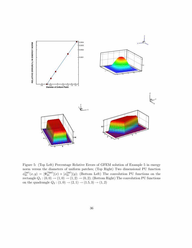
Relative Error in energy norm in percent versus the diameter of the uniform patch inlog× log scale is depicted in Fig. 5. The five relative errors in Fig. 5 are when the physicaldomain, Ω = [−1, 1]× [−1, 1], is uniformly partitioned so that it can have 9(N = 2), 16(N =3), 36(N = 5), 49(N = 6), 64(N = 7) particles, respectively.
Note that the slope of the line in Fig. 5 is about 4 (Actually, the slopes of the linesconnecting two adjacent squares in Fig. 5 are 3.95, 4.03, 4.08, 4.09, respectively). This resultsare what we expect from the error estimate ([2]).
6.2 Two dimensional PU functions for arbitrary quadrangular patches
Suppose Ω ⊂ R2 is a polygonal domain, Ωδ = (x, y) ∈ R
2 : dist(Ω, (x, y)) ≤ δ, and Ωδ ispartitioned into arbitrary quadrangular patches Qj , 1 ≤ j ≤ N, so that
each side of Qj is ≥ 2δ and Ωδ =⋃Nj=1Qj .
Then we haveN∑
j=1
[χQj(x, y)] = 1 almost everywhere in Ω.
31
Let the two dimensional normalized window function be defined by
w(l)δ×δ(x, y) = w
(l)δ (x)w
(l)δ (y)
so that its support is the square
Bδ = [−δ, δ]× [−δ, δ] and∫
Bδ
w(l)δ×δ(x, y)dxdy = 1.
Then we have
N∑
j=1
[χQj] ∗ [w(l)δ×δ](x, y) = 1 for all (x, y) ∈ Ω.
Here “ ∗ ” is the convolution defined by
∫
R2
χQj(ξ, η)w
(l)δ×δ(x− ξ, y − η)dξdη. (63)
If we write this convolution function by ψδ×δj , then ψδ×δj : 1 ≤ j ≤ N is a partition of unity
subordinate to the covering Qδj : 1 ≤ j ≤ N, where Qδ
j = (x, y) : dist(Qj , (x, y)) ≤ δ.Moreover, each convolution is a piecewise polynomial. However, the piecewise polynomial
structure is complicated unless the quadrangle Qj is a rectangle. We consider the convolutionPU functions in the following two cases:
[The case when Qj is a rectangle]If Qj is a rectangle, then ψδ×δj (x, y) is the tensor product of two convolution PU functions
constructed in section 3.2, and hence it becomes a piecewise polynomial consisting of at mostnine polynomials.
For example, let us consider the conical window function w(x) with exponent l = 3, inthe window function. Let
ws(x) =35
32w(x).
Then we have
w(l)δ (x) =
1
δws(
x
δ), where l = 3 is the exponent of (1)(not derivative order),
F (x) =
∫ x
−∞ws(t)dt =
0 : x ≤ −1,− 132(x+ 1)4
(
5x3 − 20x2 + 29x− 16)
: −1 ≤ x ≤ 1,1 : x ≥ 1
Fδ(x) =
∫
w(l)δ (x)dx = F (
x
δ).
32

Let Q be a quadrangle. Then the convolution of χQ and the scaled window function
w(l)δ×δ, l = 3, is as follows:
(
χQ ∗ w(l)δ×δ)
(x, y) =
∫
Q∩[Bδ+(x,y)]w(l)δ×δ(x− u, y − v)dudv,
which is a piecewise polynomial. Here Bδ + (x, y) is the translation of Bδ (the δ-box) by(x, y).
In particular, if Q = [a, b] × [c, d], one can show that the convolution PU functionψδ×δQ (x, y), with l = 3, can be explicitly represented by the following polynomials:
ψδ×δQ (x, y) =
Fδ(y − c) : (x, y) ∈ [a+ δ, b− δ]× [c− δ, c+ δ],Fδ(b− x)Fδ(y − c) : (x, y) ∈ [b− δ, b+ δ]× [c− δ, c+ δ],Fδ(b− x) : (x, y) ∈ [b− δ, b+ δ]× [c+ δ, d− δ],Fδ(b− x)Fδ(d− y) : (x, y) ∈ [b− δ, b+ δ]× [d− δ, d+ δ],Fδ(d− y) : (x, y) ∈ [a+ δ, b− δ]× [d− δ, d+ δ],Fδ(x− a)Fδ(d− y) : (x, y) ∈ [a− δ, a+ δ]× d− δ, d+ δ],Fδ(x− a) : (x, y) ∈ [a− δ, a+ δ]× [c+ δ, d− δ],Fδ(x− a)Fδ(y − c) : (x, y) ∈ [a− δ, a+ δ]× [c− δ, c+ δ],1 : (x, y) ∈ [a+ δ, b− δ]× [c+ δ, d− δ],0 : (x, y) /∈ Q
(64)
[The case when Qj is a non rectangular quadrangle]Suppose Qj is not a rectangle. Then the piecewise polynomial structure of ψδ×δj (x, y) is
more complicated. As the minimal angle of a quadrangle Qj gets smaller and lengths of sidesbecome different, the piecewise polynomial structure becomes increasingly complicated. Inthis case, the convolution PU function consists of more than 12 distinct polynomials.
The computer code for ψδ×δj (x, y) and its derivatives can be found in ([18]). Numericalexamples with respect to the convolution PU functions will be included in the forthcomingpaper.
Consider a rectangle Q1 = [0, 1]× [0, 2] and a non-rectangular quadrangle Q2 whose fourvertices are (1, 0), (2, 1), (1.5, 3), (1, 2). The convolution PU functions on Q1 and Q2 withrespect to δ = 0.1 are depicted in Fig. 5, from which one can observe that the graphs are
1, if (x, y) ∈ Qi and dist((x, y), ∂Qi) ≥ δ,0, if (x, y) /∈ Qi and dist((x, y), ∂Qi) ≥ δ,
for i = 1, 2. Since ‖∇(ψδ×δj )‖L∞(R2) is O(1/δ), by Theorem 6.1 of [2] and Theorem 4.1, theerror in GFEM solution with respect to the convolution PU function is bounded by the sumof local approximation errors, unless δ is unrealistically small.
33
6.3 Condition numbers of stiffness matrices in GFEM
The condition numbers of stiffness matrices in GFEM depend on the choice of PU functionand local approximation functions. However, they are generally very large (for example, see[21], [22]).
In this section, we briefly discuss the condition numbers resulted by using the proposedPU functions in GFEM. For this end, we consider the following local approximation functions.
1. (Lagrange local approximation functions)
• Let ξ0 = −1, ξ1 = −0.5, ξ2 = 1, ξ3 = 0.5, ξ4 = 1.
•
L4,k(ξ) =
4∏
i=0,i6=k
(ξ − ξi)(ξk − ξi)
, k = 0, 1, · · · , 4.
• Note that [φ(pp)gn × L4,k], k = 0, 1, · · · , 4 are linearly independent, but they do not
satisfy the Kronecker delta property. By taking tensor product, we obtain 25 twodimensional local approximation functions.
2. (Modified Lagrange local approximation functions)
• Let ξ0 = −0.75, ξ1 = −0.5, ξ2 = 1, ξ3 = 0.5, ξ4 = 0.75.
• Then the modified Lagrange interpolating function is defined by
ML4,k(ξ) = (1/Ck)4∏
i=0,i6=k
(ξ − ξi)(ξk − ξi)
, k = 0, 1, · · · , 4,
where Ck = φ(pp)gn (ξk), k = 0, 1, · · · , 4.
• Note that [φ(pp)gn ×ML4,k], k = 0, 1, · · · , 4 satisfy the Kronecker delta property and
its support is [−1, 1]. By taking tensor product, we obtain 25 two dimensional localapproximation functions related to the modified Lagrange interpolation polyno-mials.
Now we construct the GFEM approximation space spanned by 225 global basis functionsconstructed by parallel translation of these 25 local approximation functions to nine particleslocated at
(−1, 0), (0, 0), (1, 0)(−1, 1), (0, 1), (1, 1)(−1,−1), (0,−1), (1,−1)
Consider Poisson’s equation ∆u = f in [−1, 1] × [−1, 1]. The condition numbers of stiffnessmatrices of size 225× 225 for Galerkin approximation solutions of this equation are shown in
34

Table 5: The condition numbers when the approximation functions are (the simple PUfunction)×(Lagrange interpolating function), (the simple PU function)×( modified Lagrangeinterpolating function), and (the convolution PU function)×(Lagrange interpolating func-tion), respectively
Φ(4pp)g3 × Lagrange Φ
(4pp)g3 × modified Lagrange Convol PU × Lagrange
Cond Number 3.30E+14 4.18E+11 1.22E+06
the first and the second column of Table 5. The third condition number is obtained by usingthe convolution PU function in GFEM, where the domain is partitioned into 12 rectangularpatches. In this case, the dimension of the GFEM approximation space is 300.
Table 5 shows that the condition number when the convolution PU function is used ismuch smaller than that when the simple PU function is used.
An optimal choice of PU function and local approximation functions for a smaller condi-tion number will be discussed in the forthcoming paper.
AcknowledgementsWe are very grateful to referees and Professor John Osborn, editor of the special vol-
umes honoring Professor Ivo Babuska’s 80th birthday. They provided various constructivesuggestions and valuable references to enhance this paper.
Appendix
A Properties of B-splines
The B-splines, defined by 3.1, have the following properties ([10]):
1. bn ∈ Cn−1(R) is positive on (0, n+ 1) and vanishes outside this interval.
2. bn is a piecewise polynomial: it is a polynomial of degree n on each interval [k, k+1], k =0, · · · , n.
3. The B-spline of degree n is symmetric about y = (n+ 1)/2.
4. (Recurrence Relation)
bn(x) =x
nbn−1(x) +
n+ 1− xn
bn−1(x− 1). (65)
35
Diameter of Uniform Patch
RE
LA
TIV
EE
RR
OR
(%)
INE
NE
RG
YN
OR
M
0.6 0.8 1 1.2 1.4 1.6 1.8 2
0.0001
0.0002
0.0003
0.0004
-1-0.5
00.5
1
Y
-1
0
1
Z
0
0.5
1
XY
Z
X01
Y
0
1
2
Z
0
0.5
1
Y
X
Z
X1
2
Y
0
2
Z
0
0.5
1
Y
Z
X
Figure 5: (Top Left) Percentage Relative Errors of GFEM solution of Example 5 in energynorm versus the diameters of uniform patches; (Top Right) Two dimensional PU function
φ(pp)g3 (x, y) = [Φ
(4pp)g3 ](x) × [φ
(pp)g3 ](y); (Bottom Left) The convolution PU functions on the
rectangle Q1 : (0, 0)→ (1, 0)→ (1, 2)→ (0, 2); (Bottom Right) The convolution PU functionson the quadrangle Q2 : (1, 0)→ (2, 1)→ (1.5, 3)→ (1, 2)
36
5. (Convolution Property)
bn+m+1(x) =
∫
R
bm(x− y)bn(y)dy. (66)
6. (Marsden’s Identity) For x, t ∈ R,
(x− t)n =∑
k∈Z
(k + 1− t) · · · (k + n− t)bn(x− k). (67)
From Marsden identity, we have
∑
k
bn(x− k) = 1, (68)
which proves that bn is a PU shape function. Moreover, the same identity can beapplied to show the next property:
7. Any monomial xl, 0 ≤ l ≤ n can be represented by bn(x − k), k ∈ Z, and hence, theyare linearly independent.
In contrast to the B-splines, the RPP shape functions have the following features:
• The RPP shape functions are not always B-splines. However, they satisfy almost all ofthe properties of B-splines, except the positivity and the convolution property.
• The RPP shape functions satisfy the Kronecker delta property; and hence the RPPshape functions can handle essential boundary conditions more effectively than the B-spline basis functions. Moreover, by using the Kronecker delta property, one can showthat the RPP shape functions are linearly independent.
• The monomials xk, k ≤ m, are exactly interpolated by the RPP shape functions withreproducing property of order m. In other words, Definition (2) implies that, for allx, t ∈ R,
(x− t)m =∑
k∈Z
(k − t)mφ[(a,b);r;m](x− k).
that corresponds to Marsden’s indentity (67).
• Unlike B-spline, by increasing the degree of polynomial as shown in examples of section3, the regularities of RPP shape functions can go as high as we wish without increasingthe number of distinct polynomials.
• The RPP shape functions do not have the convolution property (66) that enable B-splines to have the simple exact integration.
37
B Orthogonal Polynomials with respect to the PU weight
functions
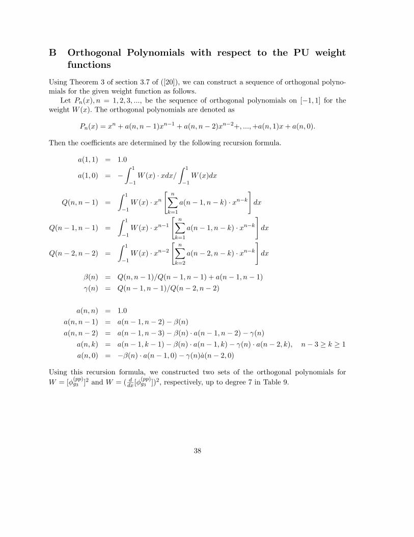
Using Theorem 3 of section 3.7 of ([20]), we can construct a sequence of orthogonal polyno-mials for the given weight function as follows.
Let Pn(x), n = 1, 2, 3, ..., be the sequence of orthogonal polynomials on [−1, 1] for theweight W (x). The orthogonal polynomials are denoted as
Pn(x) = xn + a(n, n− 1)xn−1 + a(n, n− 2)xn−2+, ...,+a(n, 1)x+ a(n, 0).
Then the coefficients are determined by the following recursion formula.
a(1, 1) = 1.0
a(1, 0) = −∫ 1
−1W (x) · xdx/
∫ 1
−1W (x)dx
Q(n, n− 1) =
∫ 1
−1W (x) · xn
[
n∑
k=1
a(n− 1, n− k) · xn−k]
dx
Q(n− 1, n− 1) =
∫ 1
−1W (x) · xn−1
[
n∑
k=1
a(n− 1, n− k) · xn−k]
dx
Q(n− 2, n− 2) =
∫ 1
−1W (x) · xn−2
[
n∑
k=2
a(n− 2, n− k) · xn−k]
dx
β(n) = Q(n, n− 1)/Q(n− 1, n− 1) + a(n− 1, n− 1)
γ(n) = Q(n− 1, n− 1)/Q(n− 2, n− 2)
a(n, n) = 1.0
a(n, n− 1) = a(n− 1, n− 2)− β(n)a(n, n− 2) = a(n− 1, n− 3)− β(n) · a(n− 1, n− 2)− γ(n)
a(n, k) = a(n− 1, k − 1)− β(n) · a(n− 1, k)− γ(n) · a(n− 2, k), n− 3 ≥ k ≥ 1
a(n, 0) = −β(n) · a(n− 1, 0)− γ(n)a(n− 2, 0)
Using this recursion formula, we constructed two sets of the orthogonal polynomials for
W = [φ(pp)g3 ]2 and W = ( d
dx [φ(pp)g3 ])2, respectively, up to degree 7 in Table 9.
38
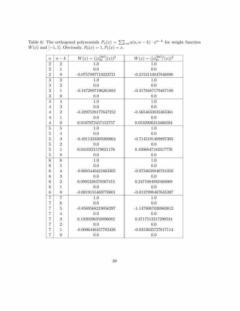
Table 6: The orthogonal polynomials Pn(x) =∑n
k=0 a(n, n − k) · xn−k for weight functionW (x) and [−1, 1]. Obviously, P0(x) = 1, P1(x) = x.
n n− k W (x) = ([φ(pp)g3 ](x))2 W (x) = ([φ
(pp)g3 ]′(x))2
2 2 1.0 1.02 1 0.0 0.02 0 -0.0757897719223721 -0.2153110047846890
3 3 1.0 1.03 2 0.0 0.03 1 -0.1872897196261682 -0.31794871794871803 0 0.0 0.0
4 4 1.0 1.04 3 0.0 0.04 2 -0.3297528177647252 -0.56546338353653614 1 0.0 0.04 0 0.0107972457152757 0.0532926313466594
5 5 1.0 1.05 4 0.0 0.05 3 -0.4911333369260064 -0.71451914098973055 2 0.0 0.05 1 0.0410221579021176 0.10068471833177765 0 0.0 0.0
6 6 1.0 1.06 5 0.0 0.06 4 -0.6685440421663305 -0.97346388467810506 3 0.0 0.06 2 0.0995238378567415 0.24710848924680696 1 0.0 0.06 0 -0.0019155469770001 -0.0137998467645397
7 7 1.0 1.07 6 0.0 0.07 5 -0.8569568219056297 -1.14790670269638127 4 0.0 0.07 3 0.1920596350896082 0.37175122172905347 2 0.0 0.07 1 -0.0096446457782426 -0.03136357276171147 0 0.0 0.0
39

References
[1] Atluri, S. and Shen, S.: The Meshless Method, Tech Science press, 2002.
[2] Babuska, I., Banerjee, U., Osborn, J.E.: Survey of meshless and generalized finite ele-ment methods:A unified appraoch, Acta Numerica, (2003) 1-125 .
[3] Babuska, I., Banerjee, U., Osborn, J.E.: Generalized finite element methods:Main Ideas,Results, and Perspectives, Int. J. of Computational Methods, Vol. 1 (2004) 67-103.
[4] Babuska, I., Banerjee, U., Osborn, J.E.: On the approximability and the selection ofparticle shape functions, Numer. math. 96 (2004) 601-640.
[5] Babuska, I., Banerjee, U., Osborn, J.E.: On principles for the selection of shape func-tions for Generalized Finite Element Method, Comput. Methods Appl. Mech. Engrg. 191(2002) 5595-5629.
[6] Ciarlet, P.G. : Basic Error Estimates for Elliptic Problems, Hanbook of NumericalAnalysis, Vol II, North Hollnad, 1991.
[7] Duarte, C.A. and Oden, J.T.: Hp clouds-a meshless method to solve boundary valeproblems, Technical Report 95-05, TICAM, The University of Texas as Austin, May1995.
[8] Duarte, C.A. and Oden, J.T.: An hp adaptive method using clouds, Comput. MethodsAppl. Mech. Engrg., Vol. 139 (1996) 237-262.
[9] Han, W. and Meng, X. :Error alnalysis of reproducing kernel particle method, Comput.Methods Appl. Mech. Engrg. 190 (2001) 6157-6181.
[10] Hollig, K : Finite Element methods with B-Spline, SIAM, 2003.
[11] Lancaster, P. and K. Salkauskas :Surfaces Generated by Moving Least Squares methods,Math. of Com., 37, pp141-158 (1981).
[12] Levin, D. :The Approximation Power of Moving Least Squares, Math. of Com., 67 (1998)1517-1531 .
[13] Li, S. and Liu, W.K. : Meshfree Particle Methods, Springer-Verlag 2004.
[14] Li, S., Lu, H., Han, W., Liu, W.K., and Simkins, D.C.Jr. :Reproducing Kernel El-ement Method: Part II. Globally Conforming Im/Cn hierarchies, Comput. MethodsAppl. Mech. Engrg., Vol. 193 (2004) 953-987.
40

[15] Liu, W.K., Han, W., Lu, H., Li, S., and Cao, J. :Reproducing Kernel Element Method:Part I. Theoretical formulation, Comput. Methods Appl. Mech. Engrg., Vol. 193 (2004)933-951.
[16] Melenk, J.M. and Babuska I. :The partition of unity finite element method:Theory andapplication , Comput. Methods Appl. Mech. Engrg. 139 (1996) 239-314.
[17] Oh, H. S., Kim, J.G., and Jeong, J. W. :The Closed Form Reproducing polynomialparticle shape functions for meshfree particle methods, Comput. Methods Appl. Mech.Engrg. 196 (2007) 3435-3461
[18] Oh, H. S., Kim, J.G., and Jeong, J. W. :The smooth piecewise polynomial particle shapefunctions corresponding to path-wise non uniformly spaced particles for meshfree particlemethods, Comput Mech 40 (2007) 569-594
[19] Oh, H.-S., Jeong, J.W., and Kim, J. G. :The Reproducing Singularity Particle ShapeFunctions for Problems Containing Singularities , Comput Mech DOI 10.1007/s00466-007-0174-x (2007)
[20] Stroud, A.H. :Numerical Quadrature and Solution of Ordinary Differential Equations,Springer-Verlag, 1974
[21] Stroubolis, T., K. Copps, and I. Babuska: Generalized Finite Element method, Comput.Methods Appl. Mech. Engrg., 190 (2001) 4081-4193.
[22] Stroubolis, T., L. Zhang, and I. Babuska: Generalized Finite Element method usingmesh-based handbooks:application to problems in domains with many voids, Comput.Methods Appl. Mech. Engrg., 192 (2003) 3109-3161.
[23] Szabo, B. and Babuska, I. , Finite Element Analysis, John Wiley, 1991.
41