the number of sidon sets and the maximum size of
TRANSCRIPT

THE NUMBER OF SIDON SETS AND THE MAXIMUM SIZE OF SIDON1
SETS CONTAINED IN A SPARSE RANDOM SET OF INTEGERS2
YOSHIHARU KOHAYAKAWA, SANG JUNE LEE, VOJTECH RODL, AND WOJCIECH SAMOTIJ3
Abstract. A set A of non-negative integers is called a Sidon set if all the sums a1+a2, with a1 ≤ a2
and a1, a2 ∈ A, are distinct. A well-known problem on Sidon sets is the determination of themaximum possible size F (n) of a Sidon subset of [n] = {0, 1, . . . , n− 1}. Results of Chowla, Erdos,Singer and Turan from the 1940s give that F (n) = (1+ o(1))
√n. We study Sidon subsets of sparse
random sets of integers, replacing the ‘dense environment’ [n] by a sparse, random subset R of [n],and ask how large a subset S ⊂ R can be, if we require that S should be a Sidon set.
Let R = [n]m be a random subset of [n] of cardinality m = m(n), with all the�nm
�subsets of [n]
equiprobable. We investigate the random variable F ([n]m) = max |S|, where the maximum is takenover all Sidon subsets S ⊂ [n]m, and obtain quite precise information on F ([n]m) for the wholerange of m, as illustrated by the following abridged version of our results. Let 0 ≤ a ≤ 1 be afixed constant and suppose m = m(n) = (1 + o(1))na. We show that there is a constant b = b(a)such that, almost surely, we have F ([n]m) = nb+o(1). As it turns out, the function b = b(a) is acontinuous, piecewise linear function of a that is non-differentiable at two ‘critical’ points: a = 1/3and a = 2/3. Somewhat surprisingly, between those two points, the function b = b(a) is constant.
Our approach is based on estimating the number of Sidon sets of a given cardinality containedin [n]. Our estimates also directly address a problem raised by Cameron and Erdos [On the number
of sets of integers with various properties, Number theory (Banff, AB, 1988), de Gruyter, Berlin,1990, pp. 61–79].
1. Introduction4
Recent years have witnessed vigorous research in the classical area of additive combinatorics. An5
attractive feature of these developments is that applications in theoretical computer science have6
motivated some of the striking research in the area (see, e.g., [32]). For a modern treatment of the7
subject, the reader is referred to [31].8
Among the best known concepts in additive number theory is the notion of a Sidon set. A set A9
of non-negative integers is called a Sidon set if all the sums a1 + a2, with a1 ≤ a2 and a1, a2 ∈ A,10
are distinct. A well-known problem on Sidon sets is the determination of the maximum possible11
size F (n) of a Sidon subset of [n] = {0, 1, . . . , n − 1}. In 1941, Erdos and Turan [12] showed12
that F (n) ≤√n + O(n1/4). In 1944, Chowla [8] and Erdos [11], independently of each other,13
observed that a result of Singer [29] implies that F (n) ≥√n−O(n5/16). Consequently, it is known14
that F (n) = (1 + o(1))√n. For a wealth of related material, the reader is referred to the classical15
Date: Fri 16th Dec, 2011, 11:32am.The first author was partially supported by CNPq (Proc. 308509/2007-2 and 484154/2010-9) and he is gratefulto NUMEC/USP, Nucleo de Modelagem Estocastica e Complexidade of the University of Sao Paulo, and ProjectMaCLinC/USP, for supporting this research. The third author was supported by the NSF grant DMS 0800070. Thefourth author was partially supported by ERC Advanced Grant DMMCA and a Trinity College JRF.Parts of this work appeared in preliminary form in SODA 2011.
1

monograph of Halberstam and Roth [15] and to a recent survey by O’Bryant [24] and the references16
therein.17
We investigate Sidon sets contained in random sets of integers, and obtain essentially tight bounds18
on their relative density. Our approach is based on finding upper bounds for the number of Sidon19
sets of a given cardinality contained in [n]. Besides being the key to our probabilistic results, our20
upper bounds also address a problem of Cameron and Erdos [7].21
We discuss our bounds on the number of Sidon sets and our probabilistic results in the next two22
subsections.23
1.1. A problem of Cameron and Erdos. Let Zn be the family of Sidon sets contained in [n].24
Over two decades ago, Cameron and Erdos [7] proposed the problem of estimating |Zn|. Observe25
that one trivially has26
2F (n)≤ |Zn| ≤
�
1≤i≤F (n)
�n
i
�= n
(1/2+o(1))√n. (1)
Cameron and Erdos [7] improved the lower bound in (1) by showing that lim supn |Zn|2−F (n) = ∞27
and asked whether the upper bound could also be strengthened. Our result is as follows.28
Theorem 1.1. There is a constant c for which |Zn| ≤ 2cF (n).29
Our proof method gives that the constant c in Theorem 1.1 may be taken to be arbitrarily close30
to log2(32e) = 6.442 · · · (for large enough n). We do not make any attempts to optimize this31
constant as it seems that our approach cannot yield a sharp estimate for log2 |Zn|. It remains an32
interesting open question whether log2 |Zn| = (1 + o(1))F (n).33
1.2. Probabilistic results. We investigate Sidon subsets of sparse, random sets of integers, that34
is, we replace the ‘environment’ [n] by a sparse, random subset R of [n], and ask how large a35
subset S ⊂ R can be, if we require that S should be a Sidon set.36
Investigating how classical extremal results in ‘dense’ environments transfer to ‘sparse’ settings has37
proved to be a deep line of research. A fascinating example along these lines occurs in the celebrated38
work of Tao and Green [14], where Szemeredi’s classical theorem on arithmetic progressions [30]39
is transferred to certain sparse, pseudorandom sets of integers and to the set of primes themselves40
(see [25, 26, 31] for more in this direction). Much closer examples to our setting are a version of41
Roth’s theorem on 3-term arithmetic progressions [27] for random subsets of integers [22], and the42
far reaching generalizations due to Conlon and Gowers [9] and Schacht [28]. For the sake of brevity,43
we shall not discuss this further and refer the reader to [9], [28], [16, Chapter 8] and [20, Section 4].44
Let us now state a weak, but less technical version of our main probabilistic results. Let F (R) =45
max |S|, where the maximum is taken over all Sidon subsets S ⊂ R. Let [n]m be a random subset46
of [n] of cardinality m = m(n), with all the�nm
�subsets of [n] equiprobable. We are interested in47
the random variable F ([n]m).48
2
a
b
1/3 2/3 1
1/3
1/2F ([n]m) = nb+o(1) for m = na
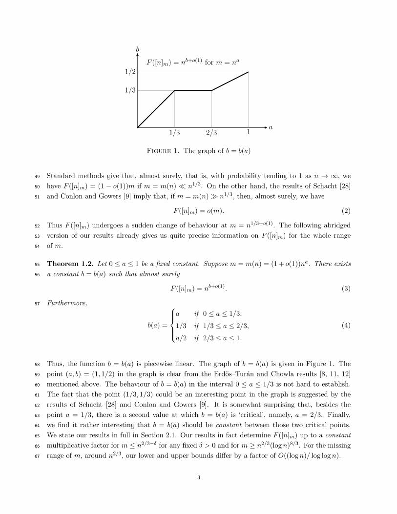
Figure 1. The graph of b = b(a)
Standard methods give that, almost surely, that is, with probability tending to 1 as n → ∞, we49
have F ([n]m) = (1 − o(1))m if m = m(n) � n1/3. On the other hand, the results of Schacht [28]50
and Conlon and Gowers [9] imply that, if m = m(n) � n1/3, then, almost surely, we have51
F ([n]m) = o(m). (2)
Thus F ([n]m) undergoes a sudden change of behaviour at m = n1/3+o(1). The following abridged52
version of our results already gives us quite precise information on F ([n]m) for the whole range53
of m.54
Theorem 1.2. Let 0 ≤ a ≤ 1 be a fixed constant. Suppose m = m(n) = (1+ o(1))na. There exists55
a constant b = b(a) such that almost surely56
F ([n]m) = nb+o(1)
. (3)
Furthermore,57
b(a) =
a if 0 ≤ a ≤ 1/3,
1/3 if 1/3 ≤ a ≤ 2/3,
a/2 if 2/3 ≤ a ≤ 1.
(4)
Thus, the function b = b(a) is piecewise linear. The graph of b = b(a) is given in Figure 1. The58
point (a, b) = (1, 1/2) in the graph is clear from the Erdos–Turan and Chowla results [8, 11, 12]59
mentioned above. The behaviour of b = b(a) in the interval 0 ≤ a ≤ 1/3 is not hard to establish.60
The fact that the point (1/3, 1/3) could be an interesting point in the graph is suggested by the61
results of Schacht [28] and Conlon and Gowers [9]. It is somewhat surprising that, besides the62
point a = 1/3, there is a second value at which b = b(a) is ‘critical’, namely, a = 2/3. Finally,63
we find it rather interesting that b = b(a) should be constant between those two critical points.64
We state our results in full in Section 2.1. Our results in fact determine F ([n]m) up to a constant65
multiplicative factor for m ≤ n2/3−δ for any fixed δ > 0 and for m ≥ n2/3(log n)8/3. For the missing66
range of m, around n2/3, our lower and upper bounds differ by a factor of O((log n)/ log log n).67
3
2. Main results68
2.1. Statement of the main results. We prove a more detailed result than Theorem 1.1.69
Let Zn(t) be the family of Sidon sets of cardinality t contained in [n].70
Theorem 2.1. Let 0 < σ < 1 be a real number. For any large enough n and t ≥ 2s0, where s0 =71 �2(1− σ)−1n log n
�1/3, we have72
|Zn(t)| ≤ n3s0
�32en
σt2
�t
. (5)
Theorem 1.1 follows from Theorem 2.1 by summing over all t (see Section 3.2). Our next result73
covers values of t smaller than the ones covered in Theorem 2.1.74
Theorem 2.2. Let n and t be integers with75
3 · 23n1/3≤ t ≤ 4(n log n)1/3. (6)
Then76
|Zn(t)| ≤
�6 · 23/2n
texp
�−
t3
3 · 27n
��t
. (7)
Let us now turn to our probabilistic results. Instead of working with the uniform model [n]m of77
random subsets of [n], it will be more convenient to work with the so called binomial model [n]p,78
in which each element of [n] is put in [n]p with probability p, independently of all other elements.79
Routine methods allow us to translate our results on [n]p below to the corresponding results on [n]m,80
where p = m/n (see Section 2.2 for details).81
We state our results on F ([n]p) split into theorems covering different ranges of p = p(n). Our first82
result corresponds to the range 0 ≤ a ≤ 1/3 in Theorem 1.2.83
Theorem 2.3. For n−1 � p = p(n) � n−2/3, we almost surely have84
F ([n]p) = (1 + o(1))np. (8)
For n−1 � p ≤ 2n−2/3, we almost surely have85
�1
3+ o(1)
�np ≤ F ([n]p) ≤ (1 + o(1))np, (9)
Remark 2.4. One may in fact prove the following result: if p = γn−2/3 for some constant γ, then86
�1−
1
12γ3 + o(1)
�np ≤ F ([n]p) ≤
�1−
1
12γ3 +
1
12γ6 + o(1)
�. (10)
Our next result covers the range 1/3 ≤ a < 2/3 in Theorem 1.2.87
Theorem 2.5. For any δ > 0, there is a positive constant c2 = c2(δ) such that if 2n−2/3 ≤ p =88
p(n) ≤ n−1/3−δ, then we almost surely have89
c1�n log(n2
p3)�1/3
≤ F ([n]p) ≤ c2�n log(n2
p3)�1/3
, (11)
4
where c1 is a positive absolute constant.90
We now turn to the point a = 2/3 in Theorem 1.2.91
Theorem 2.6. For any 0 ≤ δ < 1/3, there is a positive constant c3 = c3(δ) such that if 1 ≤ α =92
α(n) ≤ nδ and p = p(n) = α−1n−1/3(log n)2/3, then we almost surely have93
c3(n log n)1/3 ≤ F ([n]p) ≤ c4(n log n)1/3log n
log(α+ log n),
where c4 is an absolute constant.94
We remark that Theorems 2.5 and 2.6 consider ranges that overlap (functions p = p(n) of the95
form n−1/3−δ� for some 0 < δ� < 1/3 are covered by both theorems). Finally, we consider the96
range 2/3 ≤ a ≤ 1 in Theorem 1.2.97
Theorem 2.7. There exist positive absolute constants c5 and c6 for which the following holds.98
If 1 ≤ α = α(n) ≤ (log n)2 and p = p(n) = α−1n−1/3(log n)8/3, then we almost surely have99
c5√np ≤ F ([n]p) ≤ c6
√np ·
√α
1 + logα.
Furthermore, if n−1/3(log n)8/3 ≤ p = p(n) ≤ 1, then, almost surely,100
c5√np ≤ F ([n]p) ≤ c6
√np.
2.2. The uniform model and the binomial model. We now discuss how to translate Theo-101
rems 2.3, 2.5–2.7 on [n]p in Section 2.1 to the corresponding results on [n]m. Before we proceed,102
let us make the following definition.103
Definition 2.8. We shall say that an event in the probability space of the random sets [n]p or104
in the probability space of the random sets [n]m holds with overwhelming probability, abbreviated105
as w.o.p., if the probability of failure of that event is O(n−C) for any constant C, that is, if the106
probability of failure is ‘superpolynomially’ small.107
For us, the following consequence of Pittel’s inequality (see, e.g., [6, p. 35] and [17, p. 17]) will108
suffice for translating results on [n]p to results on [n]m.109
Lemma 2.9. Let 1 ≤ m = m(n) < n and p = p(n) be such that p = m/n. Let P be an event in110
the probability space of the random sets [n]p. If [n]p is in P w.o.p., then [n]m is in P ∩�[n]m
�w.o.p.111
Proof. Let Q be the complement of P . We shall show that, for any constant C > 0, there exists112
a constant C � > 0, where C � → ∞ as C → ∞, such that the following holds. If P�[n]p is in Q
�=113
O(n−C), then P�[n]m is in Q ∩
�[n]m
��= O(n−C�
).114
Pittel’s inequality (see [6, p. 35] and [17, p. 17]) states that115
P�[n]m is in Q ∩
�[n]
m
��= O(
√m) · P
�[n]p is in Q
�. (12)
5

Since, by hypothesis, P�[n]p is in Q
�= O(n−C) holds for any constant C > 0, inequality (12)116
implies that117
P�[n]m is in Q ∩
�[n]
m
��= O(
√m · n
−C) = O(√n · n
−C) = O(n−C+1/2),
which completes the proof of Lemma 2.9. �118
Every result in Theorems 2.5–2.7 will be proved with ‘w.o.p.’ rather than with ‘almost surely’.119
By Lemma 2.9, we can translate each such result on [n]p to the corresponding result on [n]m,120
where p = m/n. For example, Theorem 2.5 implies the following uniform version: For any δ > 0,121
there is a positive constant c2 = c2(δ) such that if 2n1/3 ≤ m = m(n) ≤ n2/3−δ, then, with122
overwhelming probability, we have123
c1
�n log
m3
n
�1/3
≤ F ([n]m) ≤ c2
�n log
m3
n
�1/3
,
where c1 is a positive absolute constant.124
Finally, we remark that one may use the usual deletion method to prove that the result on [n]m125
corresponding to Theorem 2.3 holds almost surely.126
2.3. Organization. Our results on the number of Sidon sets are proved in Section 3. In Section 4,127
we consider the upper bounds in Theorems 2.5–2.7. Section 5 contains some preparatory lemmas128
for the proof of Theorems 2.3 and for the proofs of the lower bounds in Theorems 2.5–2.7. The129
proof of Theorem 2.3 is given in Section 6. In Section 7, we give the proofs of the lower bounds in130
Theorems 2.5–2.7.131
For simplicity, we omit ‘floor’ and ‘ceiling’ symbols in our formulae, when they are not essential.132
For the sake of clarity of the presentation, we often write a/bc instead of the less ambiguous a/(bc).133
3. The number of Sidon sets134
The proofs of Theorems 2.1 and 2.2 are based on a method introduced by Kleitman andWinston [19]135
(see [2, 4, 5, 13, 21] for other applications of this method).136
3.1. Independent sets in locally dense graphs. We start with the following lemma, which137
gives an upper bound for the number of independent sets in graphs that are ‘locally dense’.138
Lemma 3.1. Let G be a graph on N vertices, let q be an integer and let 0 ≤ β ≤ 1 and R be real139
numbers with140
R ≥ e−βq
N. (13)
Suppose the number of edges e(U) induced in G by any set U ⊂ V (G) with |U | ≥ R satisfies141
e(U) ≥ β
�|U |
2
�. (14)
6
Then, for all integers r ≥ 0, the number of independent sets in G of cardinality q + r is at most142
�N
q
��R
r
�. (15)
Proof. Fix an integer r ≥ 0. We describe a deterministic algorithm that associates to every inde-143
pendent set I of size q + r in G a pair (S0, A) of disjoint sets with S0 ⊂ I ⊂ S0 ∪ A ⊂ V (G) and144
with |S0| = q and |A| ≤ R. Furthermore, if, for some inputs I and I �, the algorithm outputs (S0, A)145
and (S�0, A
�) with S0 = S�0, then A = A�. A moment’s thought now reveals that the number of146
independent sets in G with q+ r elements is at most as given in (15), as claimed. We now proceed147
to describe the algorithm.148
At all times, our algorithm maintains a partition of V (G) into sets S, X, and A (short for selected,149
excluded, and available). As the algorithm evolves, S increases, X increases and A decreases. The150
vertices in A will be labelled v1, . . . , v|A|, where, for every i, the vertex vi has maximum degree151
in G[{vi, . . . , v|A|}] (the graph induced by {vi, . . . , v|A|} in G); we break ties arbitrarily by giving152
preference to vertices that come earlier in some arbitrary predefined ordering of V (G).153
We start the algorithm with A = V (G) and S = X = ∅. Crucially, at all times we maintain S ⊂154
I ⊂ S ∪ A. The algorithm works as follows. While |S| < q, we repeat the following. Let a = |A|155
and suppose A = {v1, . . . , va}, with the vertex labelling convention described above. Let i be the156
smallest index such that vi belongs to our independent set I, move v1, . . . , vi−1 from A to X (they157
are not in I by the choice of i), and move vi from A to S (vi is in I). Observe that A has already158
lost i members in this iteration and S has gained one. Let U = {vi, . . . , va}. If |U | ≥ R, we further159
move all neighbours of vi in A to X (since I is an independent set and vi ∈ I). Otherwise, i.e.,160
if |U | < R, consider the first q − |S| members vi1 , . . . , viq−|S| of I ∩ A and move them from A to S161
(note that i < i1 < · · · < iq−|S| ≤ a and we now have |S| = q).162
The procedure above defines an increasing sequence of sets S. Once we obtain a set S with |S| = q,163
we let S0 = S, output (S0, A) and stop the algorithm. Inspection shows that A depends only on S0164
and not on I, i.e., if (S0, A) and (S0, A�) are both outputs by the algorithm (for some inputs I165
and I �), then A = A�. We now use our assumption on G to show that |A| ≤ R.166
We consider two cases: The first case is the case in which the body of the while loop of the algorithm167
is executed with |U | < R at an iteration. The second case is the case in which we have |U | ≥ R168
during the q iterations of the while loop. Observe that one of two cases must occur.169
First, we consider the first case. At the iteration with |U | < R, the set A lost the first i vertices170
(and possibly others) and hence at the end of this iteration we have |A| ≤ a − i = |U | − 1 < R.171
Moreover, |S| becomes of cardinality q and the algorithm stops.172
Next, we consider the second case in which we have |U | ≥ R during the q iterations of the while loop.173
In each iteration, consider an execution of the body of the while loop of the algorithm when |U | ≥ R174
and (only) the vertex vi is moved to S. In this execution, A loses, in total, i + d(vi, U) vertices,175
where d(vi, U) is the degree of vi in the graph G[U ]. Recall that we are considering the case |U | ≥ R176
7
and that vi has maximum degree in the graphG[U ]. Applying (14), we see that d(vi, U) ≥ β(|U |−1).177
Therefore, at the end of this iteration, A has cardinality178
a− (i+ d(vi, U)) ≤ a− (a− |U |+ 1 + β(|U |− 1)) ≤ |U |− β|U | ≤ (1− β)a.
In the second case, the cardinality of A decreases by a factor of 1 − β in the q iterations of the179
while loop and, at the end, A has at most N(1− β)q ≤ Ne−βq ≤ R elements. �180
3.2. Proof of Theorem 2.1. We derive Theorem 2.1 from the following lemma.181
Lemma 3.2. Let n, s and q be integers and let 0 < σ < 1 be a real number such that182
s2q
n≥
2
1− σlog
σs
2. (16)
Then, for any integer r ≥ 0, we have183
|Zn(s+ q + r)| ≤ |Zn(s)|
�n
q
��2n/σs
r
�. (17)
To obtain the bound for |Zn(t)| in Theorem 2.1, we apply Lemma 3.2 iteratively.184
Proof of Theorem 2.1. Fix integers n and t, with t ≥ 2s0, where s0 is as given in the statement185
of our theorem, that is, s0 =�2(1− σ)−1n log n
�1/3. We may clearly suppose that t ≤ F (n) =186
(1 + o(1))√n, as otherwise Zn(t) = ∅. Let K be the largest integer satisfying t2−K ≥ 2s0. We187
define three sequences (sk)0≤k≤K , (qk)0≤k≤K and (rk)0≤k≤K as follows. We let q0 = s0 and r0 =188
t2−K − s0 − q0. Moreover, we let s1 = t2−K ≥ 2s0, q1 = q0/4 and r1 = t2−K+1 − s1 − q1.189
For k = 2, . . . ,K, we let sk = 2sk−1 = t2−K+k−1, qk = qk−1/4 = q04−k and rk = t2−K+k − sk − qk.190
We apply Lemma 3.2 with parameters sk, qk and rk for k = 0, . . . ,K, to obtain from (17) that191
|Zn(t2−K+k)| = |Zn(sk + qk + rk)| ≤ |Zn(sk)|
�n
qk
��2n/σsk
rk
�(18)
for all k. It suffices to check (16) to justify these applications of Lemma 3.2. Since s2kqk ≥ s20q0 =192
2(1−σ)−1n log n > 2(1−σ)−1n log(σsk/2) for all 0 ≤ k ≤ K, inequality (16) holds for n, sk and qk.193
Using that sk = sk−1 + qk−1 + rk−1 = t2−K+k−1 for k ≥ 1 and that |Zn(s0)| ≤�ns0
�, we obtain194
from (18) that195
|Zn(t)| ≤
�n
s0
� �
0≤k≤K
�n
qk
� �
0≤k≤K
�2n/σsk
rk
�. (19)
Note that196 �n
s0
�≤
�en
s0
�s0
≤ n2s0/3 (20)
and that197 �
0≤k≤K
�n
qk
�≤ n
�0≤k≤K qk ≤ n
q0�
0≤k≤K 1/4k≤ n
4q0/3 = n4s0/3. (21)
We now proceed to estimate the last factor of the right-hand side of (19). First note that, by the198
choice of K, we have (r0 + s0 + q0)/2 = t2−K−1 < 2s0, and hence r0 < 2s0. Therefore, we have199
8
200 �2n/σs0
r0
�≤
�2en
σs0r0
�r0
≤ nr0/3 ≤ n
2s0/3 ≤ ns0 (22)
for all large n. We now note that201
�
1≤k≤K
�2n/σsk
rk
�=
�
1≤k≤K
�2n/σsK−k+1
rK−k+1
�≤
�
1≤k≤K
�2n/σsK−k+1
rK−k+1 + qK−k+1
�. (23)
To justify the inequality in (23) above, we check that202
rK−k+1 + qK−k+1 ≤2n
3σsK−k+1. (24)
Recalling that rK−k+1+qK−k+1 = sK−k+1 = t2−k, we see that (24) is equivalent to t2−k ≤�
2n/3σ.203
However,204
t
2k≤
t
2≤
1
2F (n) =
�1
2+ o(1)
�√n ≤
�2n
3≤
�2n
3σ(25)
for all large enough n. We continue (23) by noticing that205
�
1≤k≤K
�2n/σsK−k+1
rK−k+1 + qK−k+1
�=
�
1≤k≤K
�2n/σt2−k
t2−k
�≤
�
1≤k≤K
�22k+1en
σt2
�t2−k
≤
�2en
σt2
�t�
k≥1 2−k
22t�
k≥1 k2−k
=
�2en
σt2
�t
24t =
�32en
σt2
�t
. (26)
Inequality (5) now follows from (19), (20), (21), (22) and (26). �206
It now remains to prove Lemma 3.2.207
Proof of Lemma 3.2. Let S0 ⊂ [n] be an arbitrary Sidon set with |S0| = s. We show that the208
number of Sidon sets S ⊂ [n] with S0 ⊂ S and |S| = s + q + r is at most�nq
��2n/σsr
�, whence our209
lemma will follow.210
Let G be the graph on V = [n] \ S0 satisfying that {a1, a2} (a1 �= a2) is an edge in G if and only if211
there are b1 and b2 ∈ S0 such that a1+b1 = a2+b2. Observe that if S ⊂ [n] is a Sidon set containing212
S0, then S \S0 is an independent set in G. Let N = |V | = n− s, β = (1−σ)s2/2n and R = 2n/σs.213
We wish to apply Lemma 3.1 to G with β and R as just defined, to obtain an upper bound for the214
number of independent sets of cardinality q + r. Note that (13) follows from (16). Now let U ⊂ V215
with |U | ≥ R be given. We check (14) as follows.216
Let J be the bipartite graph with (disjoint) vertex classes [2n] and U , with w ∈ [2n] adjacent217
to a ∈ U in J if and only if w = a + b for some b ∈ S0. Note that a1 and a2 ∈ U have a common218
neighbour w ∈ [2n] if and only if there are b1 and b2 ∈ S0 with a1 + b1 = w = a2 + b2, that is, if219
and only if {a1, a2} is an edge of G.220
Now note that J contains no 4-cycle: if a1, a2 ∈ U with a1 �= a2 are both adjacent to both w and221
w� ∈ [2n] with w �= w�, then a1+b1 = w = a2+b2 for some b1 and b2 ∈ S0 and a1+b�1 = w� = a2+b�2222
for some b�1 and b�2 ∈ S0. But then b1 − b�1 = b2 − b�2, and hence b1 + b�2 = b�1 + b2. As b1, b�1, b2223
9
and b�2 ∈ S0 and S0 is a Sidon set, we have {b1, b�2} = {b�1, b2}. Since a1 �= a2, we have b1 �= b2,224
whence b1 = b�1, implying that w = a1 + b1 = a1 + b�1 = w�.225
The remarks above give that e(U) =�
w∈[2n]
�dJ (w)2
�, where dJ(w) denotes the degree of w in J .226
Note that�
w∈[2n] dJ(w) =�
a∈U dJ(a) = |U ||S0| = |U |s. Using the convexity of the func-227
tion f(x) =�x2
�and Jensen’s inequality and recalling that |U | ≥ R = 2n/σs, i.e., 1 ≤ σ
|U |s2n ,228
we obtain229
e(U) =�
w∈[2n]
�dJ(w)
2
�≥ 2n
�|U |s/2n
2
�=
|U |s
2
�|U |s
2n− 1
�≥
1
4(1− σ)
s2
n|U |
2≥ β
�|U |
2
�,
as required in (14). Recall that a Sidon set S ⊂ [n] containing S0 is such that S \ S0 is an230
independent set in G. Therefore, our required bound for the number of such S with |S| = s+ q+ r231
follows from the upper bound (15) for the number of independent sets of cardinality q+ r in G. �232
We conclude this section by deriving Theorem 1.1 from Theorem 2.1.233
Proof of Theorem 1.1. Let σ = 32/33 in Theorem 2.1. Then s0 = (2(1 − σ)−1n log n)1/3 =234
(66n log n)1/3. For large enough n, we have235
|Zn| =�
0≤t≤F (n)
|Zn(t)| ≤�
0≤t<2s0
�n
t
�+
�
2s0≤t≤F (n)
n3s0
�33en
t2
�t
. (27)
Note that236 �
0≤t<2s0
�n
t
�≤ 2s0
�n
2s0
�≤ n
2s0 , (28)
and that since f(t) = (33en/t2)t is increasing on the interval�0,�33n/e
�,237
�
2s0≤t≤F (n)
n3s0
�33en
t2
�t
≤√n · n
3s0(33e)√n(1+o(1))
≤ (33e)√n(1+o(1))
≤ (33e)F (n)(1+o(1)). (29)
Combining (27) together with (28) and (29) implies that |Zn| ≤ 2cF (n) for a suitable constant c. �238
3.3. Proof of Theorem 2.2. We derive Theorem 2.2 from the following more general but technical239
estimate.240
Lemma 3.3. Let n and t be integers. Suppose s is an integer and σ is a real number such that,241
letting ω = t/s, we have242
ω ≥ 4, 0 < σ < 1 ands3
n≥
2
1− σlog
σs
2. (30)
Then
|Zn(t)| ≤
�12ωn
(tσ)1−2/ωt
�t
. (31)
10
Proof. We invoke Lemma 3.2 with q = s. Note that, then, (30) implies (16). We now let r in243
Lemma 3.2 be t− 2s and obtain that244
|Zn(t)| ≤
�n
s
��n
s
��2n/σs
t− 2s
�. (32)
The right-hand side of (32) is245
�n
s
�2�2n/σst− 2s
�≤
�en
s
�2s�
2en
σs(t− 2s)
�t−2s
=�en
s
�2s �ens
�t−2s�
2
σ(t− 2s)
�t−2s
=�eωn
t
�t�
2
σt(1− 2/ω)
�t(1−2/ω)
=�C
n
t2−2/ωσ1−2/ω
�t,
where C = 21−2/ωeω/(1−2/ω)1−2/ω = 21−2/ωeω2−2/ω/(ω−2)1−2/ω. As ω ≥ 4, we have ω−2 ≥ ω/2,246
and hence C ≤ eω41−2/ω < 12ω, completing the proof of Lemma 3.3. �247
Proof of Theorem 2.2. We shall apply Lemma 3.3. Let ω = 4 and s = t/ω = t/4. Let λ =248
exp�t3/(3 · 26n)
�and set σ = 2λ/s = 8λ/t ≤ 1/3, where the last inequality follows from (6). It249
follows that 2/(1− σ) ≤ 3, and hence250
s3
n=
t3
43n= 3 log λ ≥
2
1− σlog λ,
whence the third condition in (30) holds. We thus conclude that (31) holds. Let us now estimate251
the right-hand side of (31).252
Note that tσ = 4sσ = 8λ, and therefore (tσ)1−2/ω = (8λ)1/2 and253
12ωn
(tσ)1−2/ωt=
12 · 4n
(8λ)1/2t=
6 · 8n
81/2λ1/2t=
6 · 23/2n
λ1/2t=
6 · 23/2n
texp
�−
t3
3 · 27n
�. (33)
Inequality (7) follows from (31) and (33), and Theorem 2.2 is proved. �254
4. The upper bounds in Theorems 2.5–2.7255
We shall apply Lemma 3.3 and Theorem 2.1 in order to prove the upper bounds in Theorem 2.5256
and Theorems 2.6–2.7, respectively.257
4.1. Proof of the upper bound in Theorem 2.5. Let δ > 0 be given. We show that there is a258
constant c2 = c2(δ) such that if 2n−2/3 ≤ p = p(n) ≤ n−1/3−δ, then w.o.p. we have259
F ([n]p) ≤ c2�n log n2
p3�1/3
.
To this end, we apply Lemma 3.3. We first define several auxiliary constants used to set t, ω and σ260
in Lemma 3.3. Choose η > 0 small enough so that261
(1− 3δ)
�1
3+ η
�<
1
3. (34)
11
Choose ω ≥ 4 so that262 �1
3+ η
��1−
2
ω
�>
1
3. (35)
Finally, choose c = c2 so that263
�c
ω
�3> 3
�1
3+ η
�and c >
24ω
2(1+3η)(1−2/ω). (36)
Now set t = c�n log n2p3
�1/3, s = t/ω, σ = 2(n2p3)1/3+η/s and ξ = 24ω/c2(1+3η)(1−2/ω). Note that264
t ≥ c(n log 8)1/3 ≥ cn1/3 and ξ < 1. (37)
We first check that condition (30) holds for large enough n. We have ω ≥ 4 by the choice of ω.265
Moreover, we have σ → 0 as n → ∞ because of (34). Finally, from (36) and the fact that σ → 0,266
we have267
s3
n=
�c
ω
�3log n2
p3≥ 3
�1
3+ η
�log n2
p3≥
2(1/3 + η)
1− σlog n2
p3 =
2
1− σlog
σs
2,
which completes the verification of (30). Hence Lemma 3.3 implies that268
P ([n]p contains a Sidon set of size t) ≤ |Zn(t)|pt≤
�12ωnp
t(tσ)1−2/ω
�t
. (38)
Making use of the first equation of (37) and the fact that tσ = ωsσ = 2ω(n2p3)1/3+η, we see that269
the upper bound in (38) is at most270
�12ωnp
cn1/3(2ω)1−2/ω(n2p3)(1/3+η)(1−2/ω)
�t
≤
�12ω
c(2ω)1−2/ω·
n2/3p
(n2p3)(1/3+η)(1−2/ω)
�t
=
�12ω2/ω
21−2/ωc(n2p3)(1/3+η)(1−2/ω)−1/3
�t
, (39)
which, by (35) and the assumption p ≥ 2n−2/3, is at most271
�12ω
21/2c(23)(1/3+η)(1−2/ω)−1/3
�t
≤
�24ω
c2(1+3η)(1−2/ω)
�t
= ξt. (40)
To complete the proof, it suffices to recall (37).272
4.2. Proof of the upper bound in Theorem 2.6. Suppose 1 ≤ α = α(n) ≤ n1/3, and let273
p = p(n) = α−1n−1/3(log n)2/3. We show that w.o.p.274
F ([n]p) ≤ c4(n log n)1/3log n
log(α+ log n)(41)
for some absolute constant c4. To this end, we use Theorem 2.1. Let σ = 3/4, s0 = 2(n log n)1/3275
and t = ωs0, where276
ω = 11elog n
log(α+ log n), (42)
12
and note that ω ≥ 2 for sufficiently large n. Hence, by Theorem 2.1 and the union bound, the277
probability that [n]p contains a Sidon set with at least t elements can be bounded as follows:278
P (F ([n]p) ≥ t) ≤ |Zn(t)|pt≤ n
3s0
�44enp
t2
�t
= n3s0
�44enp
ω2s20
�ωs0
≤
��11e
αω2
�ω
n3
�s0, (43)
where the last inequality follows from p = α−1n−1/3(log n)2/3 and s0 = 2(n log n)1/3.279
For the proof of (41), it suffices to show that the base of the exponential in the right-hand side280
of (43) is bounded away from 1, that is, whether281
�11e
αω2
�ω
n3< 1− ε (44)
for some absolute constant ε > 0. Since ω ≥ 11e for sufficiently large n, then we have282
�αω2
11e
�ω
≥ (αω)ω = exp (ω log(αω)) . (45)
We claim that283
2 log(αω) ≥ log(α+ log n). (46)
Observe that since ω ≥ 2, then (46) is trivially satisfied if α ≥ log n. On the other hand, if284
α ≤ log n, then ω ≥ (log n)/ log log n and hence285
2 log(αω) ≥ 2 logω ≥ 2 log log n− 2 log log log n ≥ log(2 log n) ≥ log(α+ log n).
It follows from (42), (45) and (46) that286
�αω2
11e
�ω
≥ exp (ω log(αω)) ≥ exp (5e log n) ≥ 2n3
and hence (44) holds, completing the proof of (41).287
4.3. Proof of the upper bounds in Theorem 2.7. Suppose that β = β(n) ≥ 1 and let p =288
p(n) = βn−1/3(log n)2/3. Let σ = 3/4, s0 = 2(n log n)1/3 and t = ωs0 for some ω ≥ 2. Similarly as289
in the proof of the upper bound in Theorem 2.6, see (43), using Theorem 2.1, we estimate290
P (F ([n]p) ≥ t) ≤ |Zn(t)|pt≤
��11eβ
ω2
�ω
n3
�s0. (47)
We split into two cases, depending on the order of magnitude of β.291
(Case I) If β(n) ≤ (log n)2, then we let α = β−1(log n)2 and ω = (11e log n)/ log(eα) so that292
t = ωs0 = 22e√np ·
√α/ log(eα). Note that293
�11eβ
ω2
�ω
=
�11e(log n)2
αω2
�ω
=
�(log(eα))2
11eα
�11e(log(eα))−1 logn
. (48)
13
Since the function f(x) =�
x2
11ex
�1/x= 1
e
�x2
11
�1/xis bounded by e
√4/11/e−1 = 0.459 · · · on294
the interval [1,∞), it follows from (48) that (we let x = log(eα))295
�11eβ
ω2
�ω
≤
�1
2
�11e logn
≤ n−4
,
which, together with (47), proves that w.o.p. we have296
F ([n]p) ≤ t = c6√np ·
√α
1 + logα,
where c6 is an absolute constant.297
(Case II) If β(n) ≥ (log n)2, then we let ω = 11e√β so that t = ωs0 = 22e
√np. By (47), we have298
P (F ([n]p) ≥ t) ≤�(11e)−11e
√βn3�s0
≤
�(11e)− logn
n3�s0
≤ e−s0 ,
which proves that w.o.p. we have299
F ([n]p) ≤ t = c6√np,
where c6 is an absolute constant.300
5. Nontrivial solutions in random sets301
5.1. Estimating the number of nontrivial solutions. A solution of the equation x1 + x2 =302
y1 + y2 is a quadruplet (a1, a2, b1, b2) ∈ [n]4 = [n] × [n] × [n] × [n] with a1 + a2 = b1 + b2. A303
solution (a1, a2, b1, b2) of x1 + x2 = y1 + y2 is called trivial if it is of the form (a1, a2, a1, a2) or304
(a1, a2, a2, a1). Otherwise, it is called a nontrivial solution. Let us define a hypergraph and a305
random variable that will be important for us.306
Definition 5.1. Let307
S =�{a1, a2, a3, a4} : (a1, a2, a3, a4) is a nontrivial solution of x1 + x2 = y1 + y2
�. (49)
We think of S as a hypergraph on the vertex set [n]. As usual, for R ⊂ [n], we let S[R] denote the308
subhypergraph of S induced on R. Let X be the random variable��S
�[n]p
���, that is, the number of309
hyperedges of S induced by [n]p.310
In Lemma 5.4 below, we give an estimate for X that will be used in the proof of Theorem 2.3 and311
in the proofs of the lower bounds in Theorems 2.5–2.7.312
To estimateX, we have to deal with the issue of ‘repeated entries’ in a hyperedge {a1, a2, b1, b2} ∈ S.313
Indeed, if {a1, a2, a3, a4} ∈ S, with a1 ≤ a2 ≤ a3 ≤ a4, we may have a2 = a3, but no other equality314
can occur. Hence the hypergraph S has hyperedges of size 4 and 3. Based on this, we make the315
following definition.316
Definition 5.2. For i = 3 and 4, let Si be the subhypergraph of S with all the hyperedges of size i.317
Furthermore, let Xi :=��Si
�[n]p
���.318
14
We clearly have319
S = S4 ∪ S3 and S4 ∩ S3 = ∅ (50)
and hence320
X = X4 +X3. (51)
In order to estimate X, we estimate X4 and X3 separately.321
Lemma 5.3. Fix δ > 0. The following assertions hold w.o.p.322
(i) If p ≥ n−3/4+δ, then X4 = n3p4(1/12 + o(1)).323
(ii) If p � n−1, then X3 = O(max{n2p3, n3δ}).324
We remark that the constant implicit in the big-O notation in (ii) above is an absolute constant.325
The proof of Lemma 5.3 is based on a concentration result due to Kim and Vu [18]. We shall326
introduce the Kim–Vu polynomial concentration result in Section 5.2 and prove Lemma 5.3 in327
Section 5.3. Assuming Lemma 5.3, we are ready to estimate X.328
Lemma 5.4. Fix δ > 0 and suppose p ≥ n−3/4+δ. Then, w.o.p., X = n3p4(1/12 + o(1)).329
Proof. Let X = X([n]p) be as defined in Definition 5.1 and recall (51). From the assumption330
that p ≥ n−3/4+δ, we see that the estimates for X4 and X3 given in Lemma 5.3(i) and (ii) do331
hold w.o.p. Since the inequality np � 1 yields n2p3 � n3p4 and we also have n3δ � n4δ ≤ n3p4,332
because p ≥ n−3/4+δ, we infer max{n2p3, n3δ} � n3p4, and hence, w.o.p., X3 � X4. It follows333
from (51) and the estimate in Lemma 5.3(i) that X = n3p4(1/12 + o(1)) holds w.o.p. �334
It now remains to prove Lemma 5.3. We first introduce the main tool we shall use in the proof of335
that lemma, due to Kim and Vu [18].336
5.2. The Kim–Vu polynomial concentration result. Let H = (V,E) be a hypergraph on the337
vertex set V = [n]. We assume each hyperedge e ∈ E(H) has a real weight w(e). Let [n]p be a338
random subset of [n] obtained by choosing each element i ∈ [n] independently with probability p339
and let H�[n]p
�be the subhypergraph of H induced on [n]p. Let Y be the sum of the weights of all340
the hyperedges in H�[n]p
�, i.e., Y =
�e∈H[[n]p]w(e). Kim and Vu obtained a concentration result341
for the random variable Y . We now proceed to present their result [18] (see also Theorem 7.8.1 in342
Alon and Spencer [3]).343
We start by introducing basic definitions and notation (we follow [3]). Let k be the maximum344
cardinality of the hyperedges in H. For a set A ⊂ [n] (|A| ≤ k), let YA be the sum of the weights of345
all the hyperedges inH�[n]p
�containing A, i.e., YA =
�A⊂e∈H[[n]p]w(e). Let EA = E(YA | A ⊂ [n]p)346
be the expectation of YA conditioned on the event that A should be contained in [n]p. Let Ei be347
the maximum value of EA over all A ⊂ [n] with |A| = i. Note that E0 = E(Y ). Let µ = E(Y ) and348
set349
E� = max{Ei : 1 ≤ i ≤ k} and E = max{E�
, µ}. (52)
15
Theorem 5.5 (Kim–Vu polynomial concentration inequality). With the above notation, we have,350
for every λ > 1,351
P�|Y − µ| > ak(EE
�)1/2λk�< 2e2e−λ
nk−1
,
where ak = 8k(k!)1/2.352
5.3. Proof of Lemma 5.3. We prove (i) and (ii) of Lemma 5.3 separately.353
Proof of Lemma 5.3(i). We need to show that, for p ≥ n−3/4+δ, where δ > 0 is fixed, we have354
X4 = n3p4(1/12 + o(1)) w.o.p. We first estimate the expectation µ(X4) of X4.355
Suppose {i, j, k, l} ∈ S4 with 0 ≤ i < j < k < l ≤ n − 1. Note that i + l = j + k. Let us fix356
0 ≤ i ≤ n−1. If j ≥ (n+i)/2, then l = j+k−i > 2j−i ≥ n+i−i = n, which contradicts l ≤ n−1.357
Hence we have i < j < (n+ i)/2. For fixed i and j, if k > n+ i− j − 1, then l = j + k− i > n− 1,358
which contradicts l ≤ n− 1. Therefore we have j < k ≤ n+ i− j − 1. Once i, j and k are chosen,359
the value of l is determined by the condition i+ l = j + k. Consequently,360
|S4| ∼
n−1�
i=0
(n+i)/2�
j=i
n+i−j−1�
k=j
1 =n−1�
i=0
(n+i)/2�
j=i
(n+ i− 2j) ∼ n3� 1
0
� (1+x)/2
x(1 + x− 2y)dydx ∼
1
12n3.
Hence361
µ(X4) = |S4|p4 =
�1
12+ o(1)
�n3p4. (53)
Next we apply Theorem 5.5 to prove that X4 is concentrated around its expectation µ(X4). To this362
end, we compute the quantities Ei (1 ≤ i ≤ 4) and E� and E defined in (52). We first estimate E1.363
For a ∈ [n], consider the quantity E{a}. The number of hyperedges in S4 containing a is O(n2)364
and the probability that one such hyperedge is in [n]p, conditioned on a ∈ [n]p, is p3. We conclude365
that, for any a ∈ [n], we have E{a} = O(n2p3). Consequently, E1 = max{EA : |A| = 1} = O(n2p3).366
A similar argument gives that Ei = max{EA : |A| = i} = O(n3−ip4−i) for all 1 ≤ i < 4. Therefore,367
since np � 1, we have Ei = O(n2p3) for all 1 ≤ i < 4. Also, clearly, E4 = max{EA : |A| = 4} = 1.368
Thus369
E� = max{Ei : 1 ≤ i ≤ 4} = O(max{n2
p3, 1}), (54)
and E = max{E�, µ(X4)} = O(max{n2p3, 1, n3p4}). Since p ≥ n−3/4+δ > n−3/4, we have370
E = O(n3p4). (55)
In view of (54) and (55), a simple computation implies the following:371
(Case I) If n−3/4+δ ≤ p ≤ n−2/3, then372
E� = O(1) and E = O(n3
p4). (56)
(Case II) If p ≥ n−2/3, then373
E� = O(n2
p3) and E = O(n3
p4). (57)
16
We now estimate X4 for each case separately.374
(Case I) Suppose n−3/4+δ ≤ p ≤ n−2/3. In this case, (56) implies that375
(EE�)1/2 = O(n3
p4· 1)1/2 = O(n3
p4)1/2. (58)
Set λ = (n3p4)1/12. By the assumption p ≥ n−3/4+δ, we have376
λ = (n3p4)1/12 ≥ n
δ/3. (59)
Also n3p4 ≥ n4δ � 1, and hence combining (58) and λ = (n3p4)1/12 implies that377
(EE�)1/2λ4 = O(n3
p4)1/2(n3
p4)1/3 = O(n3
p4)5/6 = o(n3
p4). (60)
Theorem 5.5 together with (59) then yields that378
P�|X4 − µ(X4)| > a4(EE
�)1/2λ4�< 2e2e−λ
n3≤ 2e2e−nδ/3
n3,
where a4 = 84(4!)1/2. Given (60), we have that w.o.p.379
X4 = µ(X4) + o(n3p4). (61)
(Case II) Suppose p ≥ n−2/3. In this case, (57) yields that380
(EE�)1/2 = O(n3
p4n2p3)1/2 = O
�n3p4
(np)1/2
�. (62)
Set λ = (np)1/12. By the assumption p ≥ n−2/3,381
λ ≥�n1/3
�1/12= n
1/36. (63)
Since np � 1, combining (62) and λ = (np)1/12 implies that382
(EE�)1/2λ4 = O
�n3p4
(np)1/2
�(np)1/3 = O
�n3p4
(np)1/6
�= o(n3
p4). (64)
Theorem 5.5 together with (63) then yields that383
P�|X4 − µ(X4)| > a4(EE
�)1/2λ4�< 2e2e−λ
n3≤ 2e2e−n1/36
n3,
where a4 = 84(4!)1/2. Given (64), we have that w.o.p.384
X4 = µ(X4) + o(n3p4). (65)
In view of (53), it follows from (61) and (65) that, for p ≥ n−3/4+δ, we have X4 = n3p4(1/12+o(1))385
w.o.p. This completes the proof of (i) of Lemma 5.3. �386
Proof of Lemma 5.3(ii). Fix δ > 0. We show that, w.o.p., X3 = O(max{n2p3, n3δ}) for p � n−1.387
First we estimate the expectation µ(X3) of X3. Since |S3| = O(n2), we have388
µ(X3) = O(n2p3). (66)
Next, we prove a concentration result for X3 applying Theorem 5.5. To this end, we estimate389
the quantities Ei (1 ≤ i ≤ 3). As in the proof of Lemma 5.3(i), one may check that E� =390
17
max1≤i≤3Ei = O(max{np2, p, 1}) and hence E = max{E�, µ(X3)} = O(max{np2, p, 1, n2p3}). By391
the assumption np � 1, we infer392
E� = O(max{np2, 1}) and E = O(max{n2
p3, 1}). (67)
Based on (67), we consider the cases p ≥ n−2/3+δ and n−1 � p ≤ n−2/3+δ separately.393
We first suppose p ≥ n−2/3+δ. From (67), we have E� = O(max{np2, 1}) and E = O(n2p3). A proof394
similar to the proofs of (61) and (65) shows that, for p ≥ n−2/3+δ, w.o.p., X3 = µ(X3) + o(n2p3).395
This together with (66) implies that for p ≥ n−2/3+δ, w.o.p.,396
X3 = O(n2p3). (68)
We now suppose n−1 � p ≤ n−2/3+δ. In this case, (67) yields that E� = O(1) and E = O(n3δ) and397
hence, setting λ = nδ/2, we have398
(EE�)1/2λ3 = O(n(3/2)δ)n(3/2)δ = O(n3δ). (69)
Theorem 5.5 with λ = nδ/2 yields399
P�|X3 − µ(X3)| > a3(EE
�)1/2λ3�< 2e2e−λ
n2≤ 2e2e−nδ/2
n2, (70)
where a3 = 83(3!)1/2. Inequality (70) together with (69) implies that, for n−1 � p ≤ n−2/3+δ,400
w.o.p., X3 = µ(X3) + O(n3δ). Since, under the assumption p ≤ n−2/3+δ, we have µ(X3) =401
O(n2p3) = O(n3δ), we infer that, for n−1 � p ≤ n−2/3+δ, w.o.p.,402
X3 = O(n3δ). (71)
Combining (68) and (71) completes the proof of (ii) of Lemma 5.3. �403
6. Proof of Theorem 2.3404
6.1. Theorem 2.3 for smaller p = p(n). We first consider the case in which n−1 � p � n−2/3.405
Proof of (8) in Theorem 2.3. Suppose n−1 � p � n−2/3. We show that (8) holds almost surely,406
using the usual deletion method. Let S, S�[n]p
�andX be as in Definition 5.1. If we delete one vertex407
from each hyperedge in S�[n]p
�, the remaining vertex set is an independent set of S
�[n]p
�, and hence408
it is a Sidon set contained in [n]p. Consequently, F ([n]p) ≥��[n]p
�� −��S
�[n]p
��� =��[n]p
�� −X. Since409
trivially F ([n]p) ≤��[n]p
��, we have��[n]p
��−X ≤ F ([n]p) ≤��[n]p
��. Note that the Chernoff bound gives410
that, for p � n−1, we almost surely have��[n]p
�� = np+o(np). Therefore, in order to show (8), it only411
remains to show thatX = o(np) almost surely. Recall thatXi is the number of edges of cardinality i412
in S�[n]p
�(i ∈ {3, 4}), and thatX = X3+X4 (see Definition 5.2 and (51)). Equations (53) and (66),413
together with n−1 � p � n−2/3, imply that E(X) = Θ(n3p4)+O(n2p3) = Θ(n3p4) = o(np). Hence414
Markov’s inequality gives that we almost surely have X = o(np), and our result follows. �415
6.2. Theorem 2.3 for larger p = p(n). We now consider the wider range n−1 � p ≤ 2n−2/3.416
18
Proof of (9) in Theorem 2.3. We have already shown that, if n−1 � p � n−2/3, then F ([n]p) =417
(1+o(1))np holds almost surely. Therefore, it suffices to show that (9) holds if, e.g., n−2/3/ log n ≤418
p ≤ 2n−2/3. We proceed as in the proof of (8), given in Section 6.1 above. We have already observed419
that |[n]p| = np(1 + o(1)) almost surely as long as p � n−1, and therefore F ([n]p) ≤ np(1 + o(1))420
almost surely in this range of p. It now suffices to recall that F ([n]p) ≥ |[n]p|−X and to prove that,421
almost surely, we have X ≤ (2/3 + o(1))np if n−2/3/ log n ≤ p ≤ 2n−2/3. But with this assumption422
on p, Lemma 5.4 tells us that, w.o.p.,423
X =1
12n3p4 + o(n3
p4) =
1
12n3p4 + o(np) ≤
�2
3+ o(1)
�np, (72)
as required. �424
7. The lower bounds in Theorems 2.5–2.7425
Let us first state a simple monotonicity result (see, e.g., [17, Lemma 1.10]) that will be used a few426
times in this section.427
Fact 7.1. Let p = p(n) and q = q(n) be such that 0 ≤ p < q ≤ 1, and let a = a(n) > 0 and428
b = b(n) > 0 be functions of n.429
(i) If F ([n]p) ≥ a holds w.o.p., then F ([n]q) ≥ a holds w.o.p.430
(ii) If F ([n]q) ≤ b holds w.o.p., then F ([n]p) ≤ b holds w.o.p.431
Statements (i) and (ii) in Fact 7.1 are, in fact, equivalent. We state them both explicitly just for432
convenience.433
7.1. Proofs of the lower bounds in Theorems 2.5 and 2.6. The lower bounds in Theorems 2.5434
and 2.6 rely on a result on independent sets in hypergraphs. Before stating the relevant result, we435
introduce some definitions. A hypergraph is called simple if any two of its hyperedges share at most436
one vertex. A hypergraph is r-uniform if all its hyperedges have cardinality r. We shall use the437
following extension of a celebrated result due to Ajtai, Komlos, Pintz, Spencer and Szemeredi [1],438
obtained by Duke, Lefmann and the third author [10].439
Lemma 7.2. Let H be a simple r-uniform hypergraph, r ≥ 3, with N vertices and average degree440
at most tr−1 for some t. Then H has an independent set of size at least441
c(log t)1/(r−1)
tN, (73)
where c = c(r) is a positive constant that depends only on r.442
We now briefly discuss how to obtain a lower bound on F ([n]p) using Lemma 7.2. Let S�[n]p
�443
be the hypergraph in Definition 5.1. Since an independent set of S�[n]p
�is a Sidon set contained444
in [n]p, independent sets in S�[n]p
�give lower bounds for F ([n]p). To apply Lemma 7.2, we shall445
obtain a simple 4-uniform subhypergraph S∗ of S�[n]p
�by deleting suitable vertices from S
�[n]p
�.446
19
Lemma 7.2 will then tell us that S∗ has a suitably large independent set, and this will yield our447
lower bound on F ([n]p). In fact, we obtain the following result.448
Lemma 7.3. There is an absolute constant d > 0 such that, for p ≥ 2n−2/3, w.o.p. F ([n]p) ≥449
d�n log(n2p3)
�1/3holds.450
Lemma 7.3 easily implies the lower bounds in Theorems 2.5 and 2.6. The proof of Lemma 7.3 will451
be given in Section 7.3.452
7.2. Proof of the lower bound in Theorem 2.7. For larger p = p(n), it turns out that, instead453
of using Lemma 7.2, it is better to make use of the fact that [n] contains a Sidon set of cardinality454
(1 + o(1))√n (see Section 1). An immediate use of this fact gives the lower bound (1 + o(1))p
√n,455
but one can, in fact, do better. The following is a particular case of a very general theorem of456
Komlos, Sulyok and Szemeredi [23].457
Lemma 7.4. There is an absolute constant d > 0 such that, for every sufficiently large m and458
every set of integers A with |A| = m, we have459
F (A) ≥ d · F ([m]).
Since the Chernoff bound gives that, for p � 1/n, we almost surely have |[n]p| = (1 + o(1))np,460
Lemma 7.4 together with F ([m]) ≥ (1 + o(1))√m gives the lower bound in Theorem 2.7. Clearly,461
to have this result with ‘w.o.p.’, it suffices to assume p � (log n)/n. There is an alternative, simple462
proof of the following fact:463
(*) if (log n)2/n � p ≤ 1/3, then, w.o.p.,464
F ([n]p) ≥
�1
3√2+ o(1)
�√np. (74)
Fact 7.1 then implies that, for p � (log n)2/n, we have, w.o.p., F ([n]p) ≥ (1/3√6 + o(1))
√np.465
Proof of (*). Let (log n)2/n � p ≤ 1/3. We shall show that (74) holds w.o.p. We define a partition466
of [n] = {0, . . . , n−1} into equal length intervals, and consider a family of intervals in the partition467
satisfying the property that, if we choose an arbitrary element from each interval, the set of chosen468
elements forms a Sidon set. We shall choose the length of the intervals so that [n]p will intersect469
each interval in a constant number of elements on average. A simple analysis of this construction470
yields that (74) holds w.o.p. The details are as follows.471
Let I = {Ii : 0 ≤ i < �n/x�} be the partition of [n] into consecutive intervals with x = �1/p�472
elements each. More precisely, let Ii = [xi, x(i+1)− 1]∩ [n] for all 0 ≤ i < �n/x�. In what follows,473
we ignore I�n/x�−1 if this interval has fewer than x elements. Let Ieven = {I0, I2, I4, . . . } ⊂ I be474
the set of all intervals with even indices and let y = |Ieven|. Note that y ≥ (1/2)�n/x� − 1 ≥475
20
(1/2)�np� − 1 = (1/2 + o(1))np. By the Chowla–Erdos result [8, 11], there exists a Sidon subset S476
of [y] with477
|S| = (1 + o(1))√y =
�1√2+ o(1)
�√np. (75)
We “identify” [y] and Ieven by the bijection i �→ I2i. Let {ai : i ∈ S} be a set of integers with ai ∈ I2i478
for all i ∈ S. We claim that {ai : i ∈ S} is a Sidon set. Suppose ai1 + ai2 = aj1 + aj2 , where i1, i2,479
j1 and j2 ∈ S. Observe that480
ai1 + ai2 ∈ I2i1+2i2 ∪ I2i1+2i2+1 and aj1 + aj2 ∈ I2j1+2j2 ∪ I2j1+2j2+1, (76)
which, together with the assumption that ai1+ai2 = aj1+aj2 , implies that i1+i2 = j1+j2. Since S481
is a Sidon set, we have {i1, i2} = {j1, j2}, whence {ai1 , ai2} = {aj1 , aj2}. This shows that {ai : i ∈ S}482
is indeed a Sidon set.483
We now consider a random set [n]p. An interval I2i (i ∈ S) is said to be occupied if I2i contains484
at least one element of [n]p. Let Iocc be the family of occupied intervals. By the above claim, we485
have F ([n]p) ≥ |Iocc|. Let us estimate |Iocc|. Note that each interval I2i (i ∈ S) is independently486
occupied with probability487
p = 1− (1− p)x = 1− (1− p)�1/p� ≥ 1− e−p(1/p−1)
≥ 1− e−1+p
≥ 1− e−2/3
> 1/3, (77)
where the third inequality follows from the assumption p ≤ 1/3. Thus, under the assumption488
(log n)2/n � p ≤ 1/3, the Chernoff bound, (75) and (77) give that, w.o.p.,489
|Iocc| = (1 + o(1))E(|Iocc|) = (1 + o(1))|S|p ≥
�1√2+ o(1)
�√np ·
1
3=
�1
3√2+ o(1)
�√np.
Recalling that F ([n]p) ≥ |Iocc|, statement (*) follows. �490
7.3. Proof of Lemma 7.3. In Lemma 7.5 below, we prove Lemma 7.3 for a narrower range of p.491
We shall then invoke monotonicity (Fact 7.1) to obtain Lemma 7.3 in full.492
Lemma 7.5. There is an absolute constant d > 0 such that, for 2n−2/3 ≤ p � n−2/3+1/15, we493
have F ([n]p) ≥ d(n log n2p3)1/3 w.o.p.494
Proof. Let S�[n]p
�, Si
�[n]p
�, X and Xi be as in Definitions 5.1 and 5.2. Recall that the size of an495
independent set of S�[n]p
�gives a lower bound on F ([n]p).496
We wish to apply Lemma 7.2. However, since S�[n]p
�may be neither simple nor uniform, we497
consider a suitable induced subhypergraph S∗ ⊂ S�[n]p
�, as discussed just after the statement of498
Lemma 7.2. We have S�[n]p
�= S3
�[n]p
�∪ S4
�[n]p
�. Let �S4 be the set of all hyperedges in S4
�[n]p
�499
that share at least two vertices with some other hyperedge in S4�[n]p
�. If we delete one vertex from500
each hyperedge of S3�[n]p
�∪ �S4, the remaining induced subhypergraph S∗ of S
�[n]p
�is both simple501
and 4-uniform. To apply Lemma 7.2 to S∗, we now estimate |V (S∗)| and the average degree of S∗.502
First we consider |V (S∗)|. Note that |[n]p|−X3−�� �S4
�� = |[n]p|−��S3
�[n]p
���−�� �S4
�� ≤ |V (S∗)| ≤ |[n]p|.503
We shall show the following two facts.504
21
Fact 7.6. Fix δ > 0 and suppose n−1+δ � p � n−1/2. We have, w.o.p., X3 = o(np).505
Fact 7.7. Fix δ > 0 and suppose n−1+δ � p � n−2/3+1/15. We have, w.o.p.,�� �S4
�� = o(np).506
Since the Chernoff bound gives that��[n]p
�� = np+ o(np) w.o.p. for p � (log n)/n, Facts 7.6 and 7.7507
imply that, w.o.p., we have508
|V (S∗)| = np(1 + o(1)). (78)
Next we consider the average degree of S∗. Owing to S∗ ⊂ S�[n]p
�, (78) and Lemma 5.4, the509
average degree 4|S∗|/|V (S∗)| of S∗ is such that, w.o.p., 4|S∗|/|V (S∗)| ≤ 4X/|V (S∗)| ≤ n2p3.510
We now are ready to apply Lemma 7.2. In view of our average degree estimate above, we set t =511
(n2p3)1/3. Given (78), Lemma 7.2 implies that, w.o.p., the hypergraph S∗, and thus S�[n]p
�, has512
an independent set of size513
c(log t)1/3
t|V (S∗)| ≥ c
�(1/3) log(n2p3)
�1/3
(n2p3)1/3np(1 + o(1)) ≥ d
�n log(n2
p3)�1/3
, (79)
for, say, d = c/2. This completes the proof of Lemma 7.5. �514
In order to finish the proof of Lemma 7.5, it remains to prove Facts 7.6 and 7.7.515
Proof of Fact 7.6. Lemma 5.3(ii) tells us that, w.o.p., X3 = O(max{n2p3, nδ}). From the assump-516
tion n−1+δ � p � n−1/2, we have both n2p3 � np and nδ � np, whence, w.o.p., X3 = o(np). �517
Proof of Fact 7.7. We give a sketch of the proof. Let P be the family of the pairs {E1, E2} of518
distinct members E1 and E2 of S4�[n]p
�with |E1 ∩ E2| ≥ 2. Observe that519
�� �S4
�� ≤ 2|P|. (80)
An argument similar to one in the proof of Lemma 5.3(ii), based on the Kim–Vu polynomial520
concentration result, tells us that |P| = O(max{E�|P|
�, nδ}) = O
�max{n4p6, nδ}
�holds w.o.p.521
From the assumption n−1+δ � p � n−2/3+1/15 = n−3/5, we have both n4p6 � np and nδ � np,522
and hence |P| = o(np) holds w.o.p. Given (80), we have, w.o.p.,�� �S4
�� = o(np). �523
In order to establish Lemma 7.3, we need to expand the range of p in Lemma 7.5 from 2n−2/3 ≤524
p � n−2/3+1/15 = n−3/5 to p ≥ 2n−2/3.525
Proof of Lemma 7.3. To complement the range of p covered by Lemma 7.5, it is enough to show526
that, say, for p ≥ n−2/3+1/16, we have, w.o.p., F ([n]p) ≥ d��n log(n2p3)
�1/3for some absolute527
constant d� > 0. Lemma 7.5 implies that, for p = n−2/3+1/16, we have, w.o.p.,528
F ([n]p) ≥ d�n log(n2
n−2+3/16)
�1/3= d
�n log(n3/16)
�1/3
= d�n(3/16) log n
�1/3> d(1/16)1/3
�n(2 log n)
�1/3= d
��n log n2
�1/3,
22
where d� = d(1/16)1/3. By Fact 7.1, we infer that, for p ≥ n−2/3+1/16, we have, w.o.p., F ([n]p) ≥529
d��n log n2
�1/3≥ d�
�n log(n2p3)
�1/3, completing the proof of Lemma 7.3. �530
Acknowledgement. The fourth author is indebted to Tomasz Schoen for drawing his attention531
to the problem of counting Sidon sets.532
References533
[1] M. Ajtai, J. Komlos, J. Pintz, J. Spencer, and E. Szemeredi, Extremal uncrowded hypergraphs, J. Combin. Theory534
Ser. A 32 (1982), no. 3, 321–335. 7.1535
[2] N. Alon, J. Balogh, R. Morris, and W. Samotij, Counting sum-free sets in Abelian groups, submitted. 3536
[3] N. Alon and J. H. Spencer, The probabilistic method, second ed., Wiley-Interscience Series in Discrete Mathe-537
matics and Optimization, Wiley-Interscience [John Wiley & Sons], New York, 2000, With an appendix on the538
life and work of Paul Erdos. 5.2539
[4] J. Balogh and W. Samotij, The number of Km,m-free graphs, Combinatorica 31 (2011), no. 2, 131–150. 3540
[5] , The number of Ks,t-free graphs, J. Lond. Math. Soc. (2) 83 (2011), no. 2, 368–388. 3541
[6] B. Bollobas, Random graphs, Academic Press Inc. [Harcourt Brace Jovanovich Publishers], London, 1985. 2.2,542
2.2543
[7] P. J. Cameron and P. Erdos, On the number of sets of integers with various properties, Number theory (Banff,544
AB, 1988), de Gruyter, Berlin, 1990, pp. 61–79. 1, 1.1, 1.1545
[8] S. Chowla, Solution of a problem of Erdos and Turan in additive-number theory, Proc. Nat. Acad. Sci. India.546
Sect. A. 14 (1944), 1–2. 1, 1.2, 7.2547
[9] D. Conlon and W. T. Gowers, Combinatorial theorems in sparse random sets, submitted, 70pp, 2010. 1.2, 1.2548
[10] R. A. Duke, H. Lefmann, and V. Rodl, On uncrowded hypergraphs, Proceedings of the Sixth International Seminar549
on Random Graphs and Probabilistic Methods in Combinatorics and Computer Science, “Random Graphs ’93”550
(Poznan, 1993), vol. 6, 1995, pp. 209–212. 7.1551
[11] P. Erdos, On a problem of Sidon in additive number theory and on some related problems. Addendum, J. London552
Math. Soc. 19 (1944), 208. 1, 1.2, 7.2553
[12] P. Erdos and P. Turan, On a problem of Sidon in additive number theory, and on some related problems, J.554
London Math. Soc. 16 (1941), 212–215. 1, 1.2555
[13] Z. Furedi, Random Ramsey graphs for the four-cycle, Discrete Math. 126 (1994), no. 1-3, 407–410. 3556
[14] B. Green and T. Tao, The primes contain arbitrarily long arithmetic progressions, Ann. of Math. (2) 167 (2008),557
no. 2, 481–547. 1.2558
[15] H. Halberstam and K. F. Roth, Sequences, second ed., Springer-Verlag, New York, 1983. 1559
[16] S. Janson, T. �Luczak, and A. Rucinski, An exponential bound for the probability of nonexistence of a specified560
subgraph in a random graph, Random graphs ’87 (Poznan, 1987), Wiley, Chichester, 1990, pp. 73–87. 1.2561
[17] , Random graphs, Wiley-Interscience, New York, 2000. 2.2, 2.2, 7562
[18] J. H. Kim and V. H. Vu, Concentration of multivariate polynomials and its applications, Combinatorica 20563
(2000), no. 3, 417–434. 5.1, 5.1, 5.2564
[19] D. J. Kleitman and K. J. Winston, On the number of graphs without 4-cycles, Discrete Math. 41 (1982), no. 2,565
167–172. 3566
[20] Y. Kohayakawa, Szemeredi’s regularity lemma for sparse graphs, Foundations of computational mathematics567
(Rio de Janeiro, 1997), Springer, Berlin, 1997, pp. 216–230. 1.2568
[21] Y. Kohayakawa, B. Kreuter, and A. Steger, An extremal problem for random graphs and the number of graphs569
with large even-girth, Combinatorica 18 (1998), no. 1, 101–120. 3570
[22] Y. Kohayakawa, T. �Luczak, and V. Rodl, Arithmetic progressions of length three in subsets of a random set,571
Acta Arith. 75 (1996), no. 2, 133–163. 1.2572
23
[23] J. Komlos, M. Sulyok, and E. Szemeredi, Linear problems in combinatorial number theory, Acta Math. Acad.573
Sci. Hungar. 26 (1975), 113–121. 7.2574
[24] K. O’Bryant, A complete annotated bibliography of work related to Sidon sequences, Electron. J. Combin. (2004),575
Dynamic surveys 11, 39 pp. (electronic). 1576
[25] O. Reingold, L. Trevisan, M. Tulsiani, and S. P. Vadhan, Dense subsets of pseudorandom sets, FOCS, 2008,577
pp. 76–85. 1.2578
[26] , Dense subsets of pseudorandom sets, Electronic Colloquium on Computational Complexity (ECCC) 15579
(2008), no. 045. 1.2580
[27] K. F. Roth, On certain sets of integers, J. London Math. Soc. 28 (1953), 104–109. 1.2581
[28] M. Schacht, Extremal results for random discrete structures, submitted, 27pp, 2009. 1.2, 1.2582
[29] J. Singer, A theorem in finite projective geometry and some applications to number theory, Transactions of the583
American Mathematical Society 43 (1938), 377–385. 1584
[30] E. Szemeredi, On sets of integers containing no k elements in arithmetic progression, Acta Arith. 27 (1975),585
199–245, Collection of articles in memory of Juriı Vladimirovic Linnik. 1.2586
[31] T. Tao and V. Vu, Additive combinatorics, Cambridge Studies in Advanced Mathematics, vol. 105, Cambridge587
University Press, Cambridge, 2006. 1, 1.2588
[32] L. Trevisan, Guest column: additive combinatorics and theoretical computer science, SIGACT News 40 (2009),589
no. 2, 50–66. 1590
Instituto de Matematica e Estatıstica, Universidade de Sao Paulo, Rua do Matao 1010, 05508–090 Sao591
Paulo, Brazil (Y. Kohayakawa)592
E-mail address: [email protected]
Department of Mathematics and Computer Science, Emory University, Atlanta, GA 30322, USA (Y. Ko-594
hayakawa, S. J. Lee and V. Rodl)595
E-mail address: [email protected], [email protected], [email protected]
School of Mathematical Sciences, Tel Aviv University, Tel Aviv 69978, Israel, and Trinity College,597
Cambridge CB2 1TQ, UK (W. Samotij)598
E-mail address: [email protected]
24