the neuron//neuron.yale.edu/ftp/neuron/neuron−erice2015.pdf using: building running analysing...

NEURONSimulator

The

Supported by NINDS

neuron.yale.edu

School of Brain Cells and Circuits; Erice 2015

General

Slides available at:

NEURON + Python

http://neuron.yale.edu/ftp/neuron/neuron−python−erice2015.pdf

http://neuron.yale.edu/neuron/static/docs/neuronpython/index.html

NEURON + Python tutorial

http://neuron.yale.edu/ftp/neuron/neuron−erice2015.pdf

Using:

Building

Running

Analysing

Where does it fit in the overall modeling process?

What kind of models?

Methods.

How is the program organized?

Published models: ModelDB.

Networks (Inhibitory Synchronization).

Where does it fit in the overall modeling process?

Physical System

Model

Representation in NEURON

Create Representation

Investigate/Explore/Control/Use Representation

Squid axon

Hodgkin−Huxley cable equations

NEURON representation

Physical System

Model

Simulation

create axonaxon { nseg = 75 diam = 100 L = 20000 insert hh}

D

4R

a

�

@

2

V

@x

2

= C

m

@V

@t

+ g

na

m

3

h � (V � E

na

) + g

k

n

4

� (V �E

k

) + g

l

� (V � E

l

)

dm

dt

= ��

m

m+ �

m

� (1�m) �

m

=

:1(V+40)

1�e

�:1(V +40)

�

m

= 4e

�(V+65)=18)

dh

dt

= ��

h

h+ �

h

� (1 � h) �

h

= :07e

�:05(V+65)

�

h

=

1

1+e

�:1(V +35)

dn

dt

= ��

n

n + �

n

� (1� n) �

n

=

:01(V+55)

1�e

�:1(V +55)

�

n

= :125e

�(V+65)=80

1

What kind of models?

Channel

Pump

Na/Ca XDiffusion

[Ca]

Ca:B

NaK

TransmitterRelease

Extracellular fieldsLinear circuitsSynapsesNetworks

Single Channels

Artificial Spiking CellsDiscrete Event Simulation

Section

Node

Segment

Membrane

v(1)v(0) v(1.5/nseg)

Membrane

Extracellularbarrier

v(1)v(0)

vext(0) vext(1)

soma(0.5)

VmVcIc

Vm

soma(0.5)

cell[0](0.5) cell[1](0.5)

Rgap

axon[0](0.5) axon[1](0.5)

R_ephaptic

soma(0.5)

VmRe2

VxAc

Vc

Ri

Ai

Acmd

synth(0.5)

AI VIc

RI

Re1

Control

eVout

R1

axon[2](0)axon[1](0)

Vm

R2

VC

gap(0.5)

B1 B2

left(0) right(0)

Close Hide

PlotWhat?

0 1 2 3 4 5

−100

−50

0

50

0 1 2 3 4 5

−100

−50

0

50Vm (mV)Vout (mV)

LincirGraph[0] for LinearCircuit[0]

Close Hide

PlotWhat?

0 1 2 3 4 5

−450

−250

−50

150

350

0 1 2 3 4 5

−450

−250

−50

150

350 control I (nA)

LincirGraph[1] for LinearCircuit[0]

Close Hide

control

e

Vout

R1Vc

R2

axon[1](1)axon[1](0)

Vm

ArrangeLabelParametersSimulate

Parameters

Source f(t)

Initial Conditions

States

New Graph

Name map

Hints

LinearCircuit[0]

How is the program organized?

Compiled

Neuron specific syntax

Interpreter

HOC

InterpreterPython

Compiled

ParameterizedEquations

Model Descriptiontranslator

Membrane ChannelSpecification

Neu

ron

spec

ific

synt

ax

Inte

rpre

ter

HO

C

Interpreter

Python

Close Hide

States Transitions Properties

Select hh state or ks transition to change properties

C C2 Ov cai

C3 O2v

O3

(0.25*C2 + O)

(0.25*C2 + O): 3 state, 2 transitions

Power 1

Fractional Conductance

C2 fraction 0.25

O fraction 1

Adjust Run

−90 −40 10 600

0.20.40.60.8

1

−90 −40 10 600

0.20.40.60.8

1aC2ObC2O

C2 + cai <−> O (a, b) (KSTrans[29])Display inf, tau

aC2O = A

ChannelBuildGateGUI[0] for ChannelBuild[0]

Close Hide

Properties

kca Density Mechanism

k ohmic ion current

ik (mA/cm2) = g_kca * (v − ek)

g = gmax * (0.25*C2 + O) * O2 * O3

Default gmax = 0 (S/cm2)

(0.25*C2 + O): 3 state, 2 transitionsO2: 2 state, 1 transitionsO3’ = aO3*(1 − O3) − bO3*O3

ChannelBuild[0] managed KSChan[0]

Close Hide

Properties

nahh0 Point Process (Allow Single Channels)

na ohmic ion current

ina (mA/cm2) = nahh0.g * (v − ena)*(0.01/area)

g = gmax * m3h1

Default gmax = 0.12 (uS)

m3h1: 8 state, 10 transitions

ChannelBuild[3] managed KSChan[3]

Close Hide

somapashhnahhkhhleak

SingleCompartmentClose Hide

SelectPointProcess

Show

nahh0[0]

at: soma(0.5)

nahh0[0]

Nsingle 0

gmax (uS) 0.12

g (uS) 6.816e−08

PointProcessManager

Close Hide

States Transitions Properties

Select hh state or ks transition to change properties

m0h0 m1h0 m2h0 m3h0

m0h1 m1h1 m2h1 m3h1

v v v

v v v

v v v v

m3h1

m3h1: 8 state, 10 transitions

Power 1

Fractional Conductance

m0h0 fraction 0

m1h0 fraction 0

Adjust Run

00.20.40.60.8

1

00.20.40.60.8

1infm0h0m1h0taum0h0m1h0

m0h0 <−> m1h0 (a, b) (KSTrans[14])Display inf, tau

am0h0m1h0 = A*x/(1 − exp(−x)) where x = k*(v − d)

ChannelBuildGateGUI[0] for ChannelBuild[3]

0 1 2 3 4 50

100

200

300

0 1 2 3 4 50

100

200

300nahh0[0].m3h1

20935 points

1.2 1.3 1.4 1.5250

260

270

280

290

1.2 1.3 1.4 1.5250

260

270

280

290nahh0[0].m3h1

1.32 1.325 1.33 1.335 1.34262

264

266

268

1.32 1.325 1.33 1.335 1.34262

264

266

268nahh0[0].m3h1

Use variable dt

Absolute Tolerance 0.001

Atol Scale Tool Details

Methods.

Use variable dt

Absolute Tolerance 0.001

Atol Scale Tool Details

VariableTimeStep

Refresh

current model type: <*ODE*> DAE

ODE model allows any method

DAE model allows implicit fixed step or daspkImplicit Fixed StepC−N Fixed StepCvodeDaspkLocal step

DAE and daspk require sparse solver, cvode requires tree solverMx=b tree solverMx=b sparse solver

2nd order threshold (for variable step)

Numerical Method Selection

Analysis Run Rescale Original

*10 /10 Hints

v 1 65 0 ca_cadifpmp 1e−06 3e−06 0 pump_cadifpmp 1e−15 1e−13 0 pumpca_cadifpmp 1e−15 3.6e−15 0 oca_cachan 1 0.053 0 n_HHk 1 0.32 0 m_HHna 1 0.053 0 h_HHna 1 0.6 0 Ves_trel 1 0.0004 0 B_trel 1 0 0 Ach_trel 1 0 0 X_trel 1 0 0

Absolute Tolerance Scale Factors

0 200 400 600 800 1000

−80

−40

0

40

0 200 400 600 800 1000

−80

−40

0

40v(.5)

3376 steps

Graph Change Text x −100 : 1100 y −92 : 52

0 200 400 600 800 1000

−3

−2

−1

0

1

0 200 400 600 800 1000

−3

−2

−1

0

1 log10(dt + 1e−9)

Graph Move Text x −100 : 1100 y −3.4 : 1.4

0 200 400 600 800 10000

1

2

3

4

5

0 200 400 600 800 10000

1

2

3

4

5 cvode.order

Graph Move Text x −100 : 1100 y −0.5 : 5.5

665 667 669 671 673 675

−80

−40

0

40

665 667 669 671 673 675

−80

−40

0

40v(.5)

Graph Pick Vector x 664 : 676 y −92 : 52

665 667 669 671 673 675

−3

−2

−1

0

1

665 667 669 671 673 675

−3

−2

−1

0

1 log10(dt + 1e−9)

Graph Move Text x 664 : 676 y −3.4 : 1.4

665 667 669 671 673 6750

1

2

3

4

5

665 667 669 671 673 6750

1

2

3

4

5 cvode.order

Graph Move Text x 664 : 676 y −0.5 : 5.5

_

na2g = .12 S/cm

.15 nA

.061 nA

mV

ms0 1 2 3 4 5

−80

−40

0

40

− 1%

.15 nA

.061 nA

mV

ms

Implicit dt=.025 ms

0 1 2 3 4 5

−80

−40

0

40 CN dt=.001 msCN dt=.025 msCVode atol = 1e−2

Iconify

File Edit Build Tools Graph Vector Window

NEURON Main Menu

Close Hide

v

Shape x −464.993 : 577.093 y −795.633 : 338.683

Close Hide

4 useful processors

Total model complexity: 28044

24 pieces

Load imbalance: 1.9%

# threads 4

Thread ParallelCache EfficientUse busy waitingMultisplit

Refresh

ParallelComputeTool[0]

Close Hide

−10 40 90 140

−80

−40

0

40

−10 40 90 140

−80

−40

0

40v(.5)

Time [ms]

at soma

v [mV]

Graph[0] x −14 : 154 y −92 : 52 Close Hide

Init (mV) −65

Init & Run

Stop

Continue til (ms) 5

Continue for (ms) 1

Single Step

t (ms) 140

Tstop (ms) 140

dt (ms) 2.3008

Points plotted/ms 40

Scrn update invl (s) 0.05

Real Time (s) 9.77

RunControl

instead of 35.4s

PostCell

PostSyn

PreCell

PreSyn

NetCon

gid = 7

CPU 2CPU 4

MPI_Allgather

0 2 4 6

t

7

ngidtgidt

1

−−−−−−

ngidtgidt

−−−−−−

0−−−−−−

n 0

.

.

.

.

.

.

cpu 3

cpu 2

cpu 1

2.8757

ngidtgidt

1

−−−−−−

2.8757

time (ms)0 50 100 150 200 250

cell

nu

mb

er

0

100

200

300

400

500

Santhakumar et al. (2005)

time (ms)

0 400 800 1200 16000

500

1000

1500

2000

2500

Davison et al., (2003)

time (ms)

0 100 200 300 400 5000

100

200

300

400

500

Bush et al., (1999)

number of processors1 2 4 8 16 32 64 128 256 512

Tru

n (

sec)

2

5

10

20

50

100

200

400


5

10

20

50

100

200

400

800

1600


2

5

10

20

50

100

200

400Beowulf 32−bit

EPFL IBM BlueGeneIBM Linux cluster

Mac G5

Beowulf 64−bit

Migliore et al (2006) J. Comput. Neurosci. 21(2):119

Strong Scaling

Weak Scaling

8 16 32 64 128

1

2

4

8

16

32

0.5

K processors

1k Conn/cell2M Cells

Run

time

(sec

)

10k Conn/cell1/4M Cells

K processors8 16 32 64 128

0.5

1

2

4

8

16

32

Run

time

(sec

)

1k Conn/cell

2M cells 32M cells

K processors8 16 32 64 128

0

10

20

30

Run

time

(sec

)

10k Conn/cell

1/4M cells

K processors

4M cells

8 16 32 64 128 0

10

20

30

Run

time

(sec

)

Allgather

Record−Replay − One Subinterval

MPI_ISend − Two Phase, Two Subinterval

DCMF_Multicast − Two Phase, Two Subinterval

Computation Time (includes queue) Argonne National LabBlue Gene/PArtificial Spiking Net

Using:

Building

Running

Analysing

Import 3−d reconstructionsDraw stylized

Shape

HomogeneousInhomogeneous

Whole cellRegionsIndividual sections

Density

...over...

Channel Distribution

Class for use in Network

Creation

Building a Cell

Single cell

Starting fromscratch

Iconify

File Edit Build Tools Graph Vector Window

NEURON Main Menu

Close Hide

About Topology Subsets Geometry Biophysics Management Continuous Create

Topology refers to section names, connections, and 2d orientation

without regard to section length or diameter.

Short sections are represented in that tool as circles, longer ones as lines.

Subsets allows one to define named section subsets as functional

groups for the purpose of specifying membrane properties.

Geometry refers to specification of L and diam (microns), and nseg

for each section (or subset) in the topology of the cell.

Biophysics is used to insert membrane density mechanisms and specify their parameters.

Management specifies how to actually bring the cell into existence for simulation.

The default is to first build the entire cell and export it to the top level

Or else specify it as a cell type for use in networks,

It also allows you to import the existing top level cell into this builder

for modification.

If "Continuous Create" is checked, the spec is continuously instantiated

at the top level as it is changed.

CellBuild[0]

single compartmentCell BuilderNetWork CellNetWork BuilderLinear CircuitChannel Builder

Topology defines section names andconnectivity.

Close Hide


soma dend

dend[1]

dend[2]

dend[3]

axon

Basename: axon

Undo Last

Click and drag toMake SectionCopy SubtreeReconnect SubtreeRepositionMove Label

Click toInsert SectionDelete SectionDelete SubtreeChange Name

Hints

CellBuild[0]

Cell subsets help to concisely specifymembrane properties.

Constant and Inhomogenous distributions

Close Hide


soma dend

dend[1]

dend[2]

dend[3]

axon

alldendritesapicalsomax

Hints

First, select,

Select

Select OneSelect SubtreeSelect Basename

then, act.

New SectionList

Selection−>SecList

Delete SecList

Change Name

Move up

Move down

Parameterized Domain Page

CellBuild[0]

Geometry is where Length, Diameter,and spatial discretization are specified.

Close Hide


somadend

dend[1]

dend[2]

dend[3]

axon

Specify Strategy

all: d_lambda dendrites: L, diam apical somax soma: area dend dend[1] dend[2] dend[3] axon: L, diam

Hints

Distinct values over subsetLdiam

Constant value over subsetLdiamareacircuit

−−−−−−−−−−−−−

Spatial Gridnsegd_lambdad_X

CellBuild[0]

Good strategy

Concise SpecNote: Compartmentalization based on medium frequency space constant is always a good idea.

oc>topology()|−| soma(0−1) ‘−−−−| dend[0](0−1) ‘−−−−| dend[1](0−1) ‘−−−−| dend[2](0−1) ‘−−| dend[3](0−1) ‘−−−−−−| axon(0−1)

Close Hide


somadend

dend[1]

dend[2]

dend[3]

axon

Specify Strategy

all: d_lambda dendrites: L, diam soma: area axon: L, diam

Hints

forsec all { ...

// lambda_w(f)^2 = diam/(4*PI*f*Ra*cm)

// nseg = ~L/(d_lambda*lambda_w(100))

// fraction of space constant at 100Hz

d_lambda 0.1

}

CellBuild[0]

Sprinkling channels onto the cell beginswith a strategy.

Close Hide


somadend

dend[1]

dend[2]

dend[3]

axon

Specify Strategy

all: manage ...dendrites: manage ...apicalsomax: manage ... soma dend dend[1] dend[2] dend[3] axon

Hints

forsec somax { //specifyRacmpasextracellularhh

CellBuild[0]

... and ends by specifying a few parametersas constant over a few subsets.

(Inhomogeneities are a bit more complicated)

Close Hide


somadend

dend[1]

dend[2]

dend[3]

axon

Specify Strategy

all Ra cm dendrites pas somax hh

Hints

forsec somax { insert hh

gnabar_hh (S/cm2) 0.12

gkbar_hh (S/cm2) 0.036

gl_hh (S/cm2) 0.0003

el_hh (mV) −54.3

CellBuild[0]

The cell comes into existence when"Continuous Create" is turned on.(Windows derive from NEURONMainMenu "Tools" and "Graph".)


Specify Strategy

all Ra cm dendrites

forsec all { // specify cm

cm (uF/cm2) 1

CellBuild[0]

Init (mV) −65

Init & Run

Stop

Continue til (ms) 5

Continue for (ms) 1

Single Step

t (ms) 2

Tstop (ms) 5

dt (ms) 0.025

Points plotted/ms 40

Scrn update invl (s) 0.05

Real Time (s) 0

RunControl

v

Shape Space Plot x −218.462 : 323.998 y −181.944 : 257.108

−200 −100 0 100 200 300

−80

−40

0

40

−200 −100 0 100 200 300

−80

−40

0

40v

Graph[1] x −251.784 : 369.625 y −92 : 52

0 1 2 3 4 5

−80

−40

0

40

0 1 2 3 4 5

−80

−40

0

40v(.5)

Graph[2] x −0.5 : 5.5 y −92 : 52

SelectPointProcess

Show

IClamp[0]

at: dend[0](0.3)

PointProcessManager

Using the cell in a network takes three steps. 1) Encapsulate in class so many cells can be created with the same type.2) Specify the location of the output spike detector.

Close Hide


soma dend

dend[1]

dend[2]

dend[3]

axon

Cell Type Export Import Hints

This is necessary only if the cell is used in a network

This creates a file that declares a cell type

with the current specification

Such a cell class is usable in networks and

can be employed by the network builder tool.

Classname

Pyramid

Select Outputaxon.v(1)

Save hoc code in file

CellBuild[0]

3) Sprinkle synapses that can receive input spikes.

A NetworkReadyCell needs to be able tosend and receive spikes.

Close Hide

Info Refresh Cell Name: Pyramid Locate

soma dend

dend[1]

dend[2]

dend[3]

axon

ANG

A0N1

A3

N4

Synapse G at dend[3](0.5)

G

NetReadyCellGUI[0]

Use NEURONMainMenu/Tools/Miscellaneous/Import3D.Export to Cell Builder.

Starting from a 3−D Reconstruction.

Close Hide

Line 85: ( −229.03 −409.32 2.95 0.11) ; 3, 3

./030304A.ascFile format: Neurolucida V3

−−−−−−−−−−−−−−−−−−−−−−−−−−−−−−−ZoomTranslate Rotate (about axis in plane)Rotate 45deg about y axisRotated (vs Raw view)Show PointsShow Diam

Show distal (tree) from selected point

View type

Select point

Line# 85

−−−−−−−−−−−−−−−−−−−−−−−−−−−−−−−

Edit

Export

Neurolucida V3 filter facts

Import3d_GUI[0]

Close Hide

Line 85: ( −229.03 −409.32 2.95 0.11) ; 3, 3

Select point x −252.45 : −215.29 y −439.697 : −381.172

But don’t forget to compartmentalize with dlambda.

Import3D export to CellBuild−−−automaticallygives Topology, Geometry, and some Subsets.

Close Hide


somaaxondendapic

allsomaticaxonalbasalapical

Hints

First, select,

Select

Select OneSelect SubtreeSelect Basename

then, act.

New SectionList

Selection−>SecList

Delete SecList

Change Name

Move up

Move down

Parameterized Domain Page

CellBuild[0]

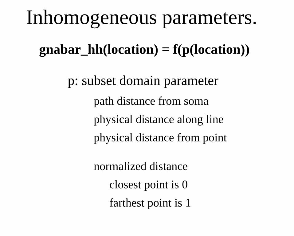
Inhomogeneous parameters.

gnabar_hh(location) = f(p(location))

p: subset domain parameter

path distance from soma

physical distance along line

physical distance from point

normalized distance

farthest point is 1

closest point is 0

The subset domain parameter defines avalue at every location on the subset.

Close Hide


p=0.902366apic[32] (0.880567)

allsomaticaxonalbasalapical apical_x

Hints

Parameterized Domain Specification

Return to Subset Selection Page

Path Length from root

translated so most proximal end at 0

and normalized so most distal end at 1

ranges from 0 to 1

Show domain valuemetric proximal distal

Remove

CellBuild[0]

...and arbitrary functions of that parametercan be used to specify a range variable.

Close Hide


p=0.202892apic[26] (0.196004)

f(p)=0.0797108

Specify Strategy

all Ra cm somatic hh axonal hh basal pas apical hh apical_x gnabar_hh

Hints

/* p is Path Length from root

translated so most proximal end at 0

and normalized so most distal end at 1

and ranges from 0 to 1 */

for apical_x.loop(&x, &p) {

gnabar_hh(x) = f(p)

}

f(p) show

f(p) = b + m*p/(p1 − p0)

b 0.1

m −0.1

CellBuild[0]

It’s always a good idea to checkthat expectations are met.

Close Hide

File

167 sections; 945 segments

* 1 real cells * root soma 167 sections; 945 segments * 15 distinct values of nseg * 6 inserted mechanisms Ra = 80 cm = 1 * pas ena = 50 ek = −77 * hh * 80 gnabar_hh 80 or more distinct values gkbar_hh = 0.036 gl_hh = 0.0003 el_hh = −54.3 * 4 subsets with constant parameters * 79 sections with unique parameters

ModelView[2]

Close Hide

LengthScale SpacePlot

gnabar_hh

0.20.1833330.166667 0.150.1333330.116667 0.10.08333330.0666667 0.050.03333330.0166667 0

0 170 340 510 680 8500

0.04

0.08

0.12

0 170 340 510 680 8500

0.04

0.08

0.12gnabar_hh

ModelView[2] Range Graph

Networks (Inhibitory Synchronization).

0 20 40 60 80 1000

0.2

0.4

0.6

0.8

1

NET_RECEIVE (w) { m = minf + (m − minf)*exp(−(t − t0)/tau) t0 = t if (flag == 0) { m = m + w if (m > 1) { m = 0 net_event(t) } net_move(t+firetime()) }else{ net_event(t) m = 0 net_send(firetime(), 1) }}

FUNCTION firetime() { : m < 1 < minf firetime = tau*log((minf−m)/(minf − 1))}

: dm/dt = (minf − m)/tau: input event adds w to m: when m = 1, or event: makes m >= 1, cell fires: minf is calculated so: that the natural interval: between spikes is invl

INITIAL { minf = 1/(1 − exp(−invl/tau)) m = 0 t0 = t net_send(firetime(), 1)}

0 100 200 300 400 5000

10

20

30

40

0 100 200 300 400 5000

10

20

30

40Cell[39]Cell[38]Cell[37]Cell[36]Cell[35]Cell[34]Cell[33]Cell[32]Cell[31]Cell[30]Cell[29]Cell[28]Cell[27]Cell[26]Cell[25]Cell[24]Cell[23]Cell[22]Cell[21]

Number of all to all cells 40

All to all connection weight 0

Delay (ms) 0

Cell time constant (ms) 10

Lowest natural interval 10

Highest natural interval 15

0 100 200 300 400 5000

10

20

30

40

0 100 200 300 400 5000

10

20

30



All to all connection weight −0.05

Delay (ms) 0




0 100 200 300 400 5000

10

20

30

40

0 100 200 300 400 5000

10

20

30



All to all connection weight −0.05

Delay (ms) 9




200 220 240 260 280 300

−1

−0.5

0

0.5

1

200 220 240 260 280 300

−1

−0.5

0

0.5

1

IntervalFire[0].M

IntervalFire[39].MIntervalFire[20].M

Published models: ModelDB.

the neuron//neuron.yale.edu/ftp/neuron/neuron−erice2015.pdf using: building running analysing...

Documents