. .. ..

THE NEAR-EARTH METEOROID ENVIRONMENT

Hztntsuille, Ala.

N A T I O N A L AERONAUTICS AND

by Robert J. Naztmann

George C, Marshall Space Flight Center

SPACE A D M I N I S T R A T I O N W A S H I N G T O N , 0. C. NOVEMBER 1966

https://ntrs.nasa.gov/search.jsp?R=19670001471 2019-03-14T18:47:24+00:00Z

TECH LIBRARY KAFB, NM

I 111111 lllll Ill1 11111 ll lllll Ill1 Ill1 Ill1 0330575

NASA TN D-3717

THE NEAR-EARTH METEOROID ENVIRONMENT

By Robert J. Naumann

George C. Marsha l l Space Flight Center Huntsville, Ala.

N A T I O N A L AERONAUTICS AND SPACE ADMINISTRATION

Far sale by the Clearinghouse for Federal Scientific and Technical Information Springfield, Virginia 22151 - Price $2.00

I

TABLE O F CONTENTS

Page

SUMMARY . . . . . . . . . . . . . . . . . . . . . . . . . . . . . . . . . . . . . i

INTRODUCTION AND APPROACH . . . . . . . . . . . . . . . . . . . . . . 2

FUNDA ME NTA L RE L A TIONS . . . . . . . . . . . . . . . . . . . . . . . . 4

DENSITY AND VELOCITY DISTRIBUTION . . . . . . . . . . . . . . . 7

OBSERVATIONAL DATA . . . . . . . . . . . . . . . . . . . . . . . . . . . . 9

Satellite Penetration Measurements . . . . . . . . . . . . . . . . 9

Explorer XVT . . . . . . . . . . . . . . . . . . . . . . . . . . . . 11 Explorer XXTII . . . . . . . . . . . . . . . . . . . . . . . . . . . . 12 Pegasus . . . . . . . . . . . . . . . . . . . . . . . . . . . . . . . . 12

Radar Observations . . . . . . . . . . . . . . . . . . . . . . . . . . . 13 Photographic Observations . . . . . . . . . . . . . . . . . . . . . . 14

COMPUTATIONPROCEDURE . . . . . . . . . . . . . . . . . . . . . . . . 15

PENETRATIONFREQUENCY . . . . . . . . . . . . . . . . . . . . . . . . 23

MASS DISTRIBUTION . . . . . . . . . . . . . . . . . . . . . . . . . . . . . . 27

COMPARISONS WITH OTHER EXPERIMENTS . . . . . . . . . . . . . 32

.

I

CONCLUSIONS . . . . . . . . . . . . . . . . . . . . . . . . . . . . . . . . . . 35

REFERENCES . . . . . . . . . . . . . . . . . . . . . . . . . . . . . . . . . . 37

iii

Figure

LIST O F ILLUSTRATIONS

Title Page

The Velocity Probability Density Function Obtained by Dohnanyi . . . . . . . . . . . . . . . . . . . . . . . . . . . . . . . . . . . . . . . 10

The Relative Abundances Assumed for the Various Representative D e n s i t i e s . . . . . . . . . . . . . . . . . . . . . . . . . . . . . . . . . . . . . . . 10

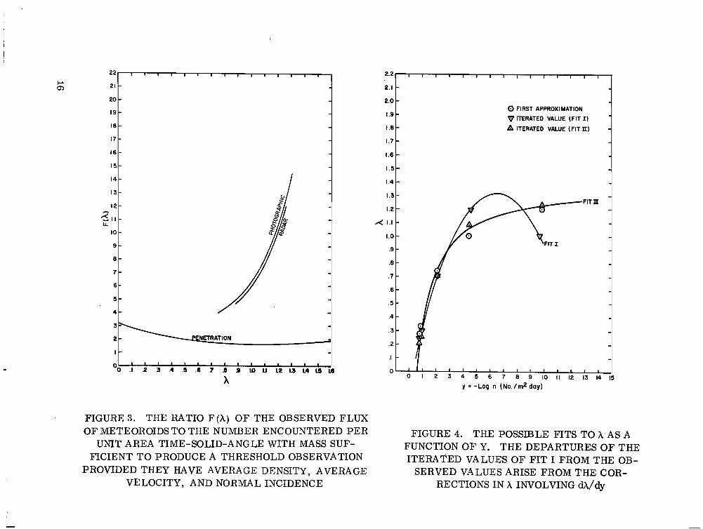
The Ratio F ( A ) of the Observed Flux of Meteoroids to the Number Encountered Per Unit Area Time-Solid-Angle with Mass Sufficient to Produce a Threshold Observation Provided They Have Average Density, Average Velocity, and Normal Incidence . . . . . . . . . . . 16

The Possible Fits to h as a Function of y. Iterated Values of Fit I From the Observed Values Arise From the Corrections in h Involving dh/dy . . . . . . . . . . . . . . . . . . . . . . . 16

The Departures of the

The Cumulative Mass Flux Distribution that Best Fits the Estimated Characterist ic Mass for Each Measurement. the Radar Points in the Vicinity of Uncertainty of the Dependence of Ionization Efficiency on

The E r r o r Bar s on gm Indicate the Result of

. . . . . . . . . . . . . . . . . . . . . . . . . . . . . . . . . . . . . . . . Velocity 22

Estimated Penetration Frequency in Various Thicknesses of 2024 -T3 A l . certainties in Mass Dependence and Form of Functional Fits. The Indicated Measurements are Penetration Rates Estimated on the Basis of the Calculated Characterist ic Mass for Each Measurement 24

The Envelope Represents Limits of Combined Un-

. . . . . . . . . . . . . . . . . . . . . . . . . . . . . . . . . . . .

An Expanded Region of the Penetration Curve. Points and the 0. 038 mm Pegasus Point were Adjusted in Thick- ness to Agree with the Slope of the Penetration Curve. Resulting Value is Taken as the Equivalent Thickness in 2024-T3 A1 . . . . . . . . . . . . . . . . . . . . . . . . . . . . . . . . . . . . . . . . . . . 30

The Explorer

The

The Directional Mass Flux Probability Density Function Compared with Estimates Obtained from Zodiacal Lightby Vande Hulst . . . . 30

iv

. . .... - . . . . . .-.I-., .. -

LIST OF TABLES

Page

TableIa . . . . . . . . . . . . . . . . . . . . . . . . . . . . . . . . . . . . . . . . . . . . 20

Table . . . . . . . . . . . . . . . . . . . . . . . . . . . . . . . . . . . . . . . . . . . . . . 21

T a b l e I I . . . . . . . . . . . . . . . . . . . . . . . . . . . . . . . . . . . . . . . . . . . . 25

V

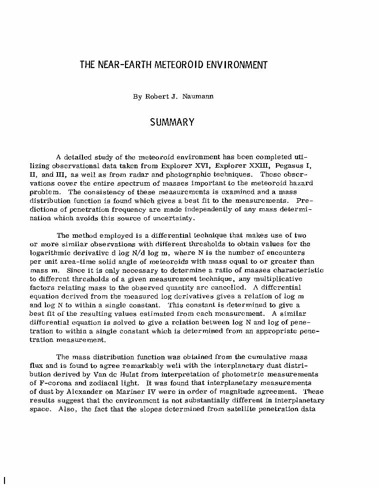
THE NEAR-EARTH METEOR0 I D ENVIRONMENT

By Robert J. Naumann

SUMMARY

A detailed study of the meteoroid environment has been completed uti-

These obser- lizing observational data taken from Explorer XVI, Explorer XXIII, Pegasus I, 11, and 111, as well as from radar and photographic techniques. vations cover the entire spectrum of masses important to the meteoroid hazard problem. distribution function is found which gives a best f i t to the measurements. Pre- dictions of penetration frequency are made independently of any mass determi- nation which avoids this source of uncertainty.

The consistency of these measurements is examined and a mass

The method employed is a differential technique that makes use of two or more similar observations with different thresholds to obtain values for the logarithmic derivative d log N/d log m y where N is the number of encounters per unit area-time solid angle of meteoroids with mass equal to or greater than mass m. to different thresholds of a given measurement technique, any multiplicative factors relating mass to the observed quantity are cancelled. A differential equation derived from the measured log derivatives gives a relation of log m and log N to within a single constant. This constant is determined to give a best fit of the resulting values estimated from each measurement. A s imilar differential equation is solved to give a relation between log N and log of pene- tration to within a single constant which is determined from an appropriate pene- tration me as ure ment .

Since it is only necessary to determine a ratio of masses characterist ic

The mass distribution function was obtained from the cumulative mass flux and is found to agree remarkably well with the interplanetary dust distri- bution derived by Van de Hulst from interpretation of photometric measurements of F-corona and zodiacal light. It was found that interplanetary measurements of dust by Alexander on Mariner IV were in order of magnitude agreement. These results suggest that the environment is not substantially different in interplanetary space. Also, the fact that the slopes determined from satellite penetration data

appear to rapidly approach zero as N increases, suggests an upper limit on number of meteoroid encounters which appear to be on the o rde r of 3/m2 day regardless of size. mands that a meaningful meteoroid experiment must expose an area on the order of a m2 to collect a good statistical sample in a reasonable time.

This low value for the maximum encounter frequency de-

The frequency of penetrations predicted from the analysis is much smaller for very thin material (< 0.0025-cm A l ) than any previous estimate. However, the number of penetrations predicted for materials > 0. 04-cm A1 is more nearly approximated by the more pessimistic previous estimates. is little doubt that the meteoroid hazard is indeed significant for vehicles with large exposures (area-time product) and that considerable emphasis must be placed on meteoroid protection in the design of such vehicles.

There

INTRODUCTION AND APPROACH

A detailed study of the meteoroid environment has been completed uti- lizing observational data taken from Explorer XVI, Explorer XXIII, Pegasus I, 11, and 111, as well as from radar , and photographic techniques. These obser- vations cover the entire spectrum of masses important to the meteoroid hazard problem. The consistency of these measurements is examined and a mass dis- tribution function is found which gives a best fi t to the measurements. Predic- tions of penetration frequency are made independently of any mass determination which avoids this source of uncertainty.

The usual approach for obtaining a meteoroid hazard model f i rs t attempts

Since there is no direct means for measuring mass of a meteoroid, such to obtain a mass f lux relation by interpreting various observations in t e rms of mass. information must be inferred from observables such as penetration in known material, electron trail density, o r emission of light. strongly dependent on velocity and other parameters which are not accurately known. an order of magnitude. several empirical penetration formulas to the mass distribution to obtain a depth of penetration in a particular material.

Such observables are also

The overall uncertainty in mass determination is estimated to be about The problem is then compounded by applying one of

The present approach makes a more direct use of the observational data and does not require specification of mass for any observation, thus avoiding the

2

I

major source of uncertainty. in the equations relating mass to the observed quantities. theoretical justification for the values of these exponents, although in some cases empirical values have been found that differ slightly from the theoretical values. The method employed is a differential technique that makes use of two o r more s imilar observations with different thresholds to obtain values for the logarithmic derivative d log N/d log m. It is important to distinguish between the observed number of incidents per unit area-time with mass, velocity, density, etc. , such that the observed quantity is above the threshold of observation, and the number N incident pe r unit area-time-solid angle with mass equal to or greater than some characterist ic value. function of d log N/d log m and contains integrations over angular, velocity, and density distributions. Fortunately, since present knowledge of such distributions is at best sketchy, they only enter in these correction t e r m s , and therefore exer t only a minor influence on the final result.

It is necessary only to know the exponent of mass There is some

These quantities are related by a factor which is a

Since it is desirable to avoid the necessity of determining mass for any observation, the logarithmic derivatives a r e specified at values of log N, which are taken as the mean of the logarithms of the fluxes that determine a particular log derivative. In this manner, a set of values for the log derivative and log N are found from the observations from which a functional relation F (log N) may be found by the method of least squares. The resulting differential equation

may be integrated to give

By the previous assumption that the observable, in this case penetration of a thickness p of some specified material, is related to mass by

log p = K + y log m (3)

where K is an undetermined constant containing velocity, density, and material property t e rms and y is the known exponent of mass in the equation relating mass to the observable. Therefore,

lo + const. log' = F (lo: N) (4)

3

Assuming the velocity and density distributions are independent of mass ,

The constant of integration which which appears to be at least approximately the case, the above equation holds over the range for which F (log N) is known. contains all the uncertainties in the definition of mass , velocity, density, and material properties may be determined by a single experiment which yields a value of N for known p of a given material. The 0.4-mm Pegasus datum point is used to obtain this constant and the derived frequency of penetration versus thickness of material applies to 2024-T3 A1 backed by a soft foam.

The mass distribution function is found from the cumulative encounter frequency N. gives a relation of log m and log N to within a single constant. This constant is determined to give a best f i t of the resulting values estimated from each meas- urement. This obviously does require the assumption of velocity and density distributions, and is also subject to e r r o r s in mass determination. However, since all the measurements are combined to find only one constant, hopefully some of these e r r o r s are averaged out, and the result is a mass distribution that is most consistent with the entire data set.

The differential equation derived from the measured log derivatives

FUNDAMENTAL RELATIONS

Unfortunately, none of the present measurement techniques directly measure meteoroid mass. that is related to mass by an observational equation of the form

All such measurements have an observed quantity Q

log Q = log K + CY log p + p log v + y log m + 6 log cos 8 (5)

where K is a constant, p the meteoroid density, v the meteoroid velocity, m the mass , and 8 the angle of incidence. thickness of the detector; for radar observations, Q is the electron t ra i l density; and for photographic meteors, Q is the intensity or the photographic magnitude.

For penetration experiments, Q is the

Because of the spectrum of velocities, densities, and angles of incidence, there is no unique value of m corresponding to Q. a given threshold Q is

The observed frequency for

00

rp = s s dS2 dp 7 d v 7 dm cos 8 n ( p ) n (v) nm(m) (6) P V 27r 0 0 m ( ~ , P , V, e )

4

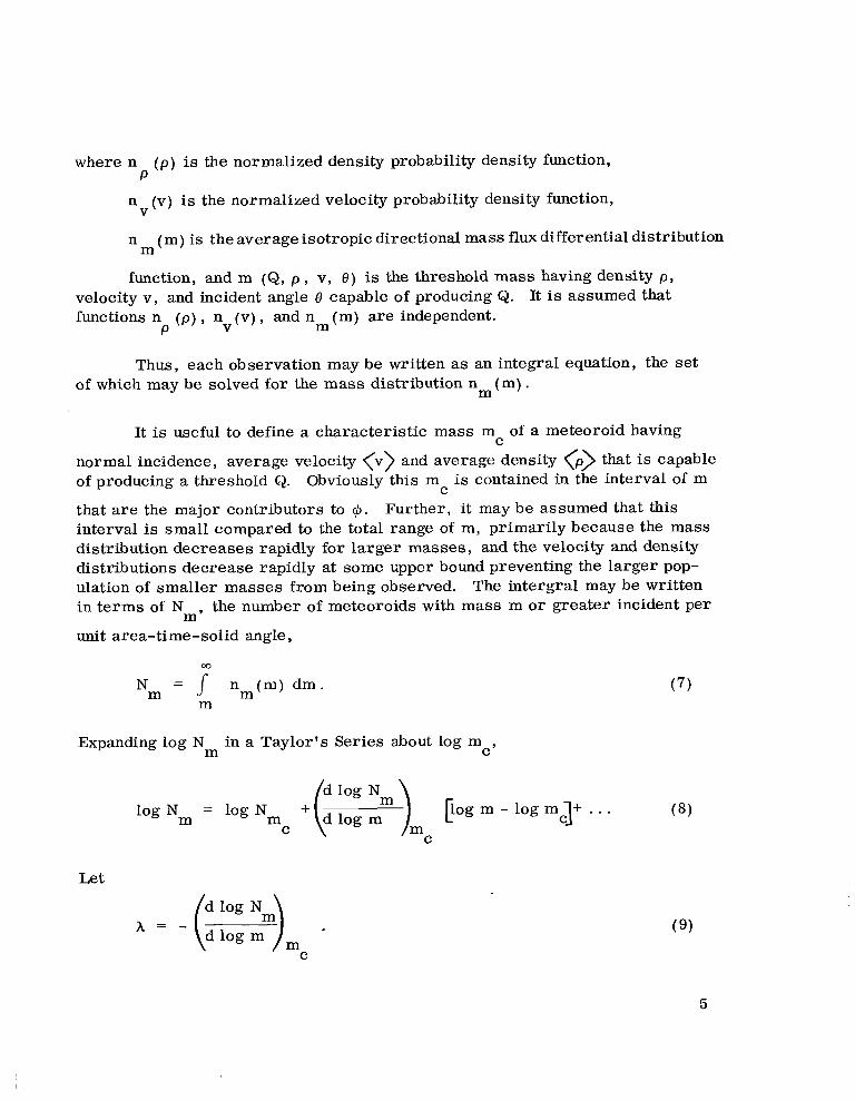
where n ( p ) is the normalized density probability density function,

n (v) is the normalized velocity probability density function,

n

function, and m (Q, p , v, e ) is the threshold mass having density p , It is assumed that

P

V

( m ) is the average isotropic directional mass flux differential distribution m

velocity v , and incident angle 8 capable of producing Q. functions n ( p ) , n (v) , and n (m) a r e independent.

V m P

Thus, each observation may be written as an integral equation, the set of which may be solved for the mass distribution n (m) . m

It is useful to define a characteristic m a s s m of a meteoroid having C

normal incidence, average velocity <v> and average density (p> that is capable of producing a threshold Q.

that are the major contributors to $. interval is small compared to the total range of m, primarily because the mass distribution decreases rapidly for larger masses , and the velocity and density distributions decrease rapidly at some upper bound preventing the larger pop- ulation of smaller masses from being observed. The intergral may be written in t e r m s of N

unit a r e a- ti me -solid angle,

Obviously this m is contained in the interval of m C

Further, it may be assumed that this

the number of meteoroids with mass m o r greater incident per m'

N = n ( m ) d m . m m m

Expanding log N in a Taylor's Series about log m m C Y

( 7 )

Let

A = - ( d log N m) ,

d l o g m C

(9)

5

The minus sign is introduced for convenience so that h will be a positive quantity.

Then A 00

J m nm (m) dm (>) N m C

The observed flux C#J may be written in te rms of N

solid angle of mass m

the incidence flux per unit m C

o r greater C

Integrating ,

where m from its definition, is c y

The factors appearing in the relation between incident flux and observed flux may be combined into a correction term

6

The first factor is an obliqueness correction which accounts for angles of incidence other than normal. The density and velocity te rms adjust the observations ac- cording to the contributions mass m .

C

Finally, the number

from the observed flux by

N = @ / F ( h ) . m

from masses above and below the characterist ic

incident having mass m o r greater may be obtained C

(15)

The quantity X must be found from the log derivative

d log F ( h ) + d log $I d log N

" = - = - d l o g m d log m d log m

This may be solved by the method of successive approximations using as a f i r s t approximation

where Q1 and $I2 are measured ra tes which correspond to observables Qiand Q2

for which the same observational equation applies, and y is the mass exponent in the observational equation.

DENSITY AND VELOCITY D ISTRIBUTION

The determination of a velocity distribution for meteors has been prob- lematic because of the strong dependence of the observable on velocity. results in a distortion of the observed velocity distribution because of the con- tribution of the more numerous smaller meteors on the high velocity end of the spectrum. Orrok in which observations are categorized into groups of constant mass de- termined from

This

One method of eliminating this selection effect was proposed by

I

where T~ is the luminous efficiency, T is the lifetime, and I the measured in- tensity. Taking a group having sufficient mass to insure practically all of the slower meteoroids will be obse'rved should give a reasonably unbiased set of data from which a velocity distribution can be obtained.

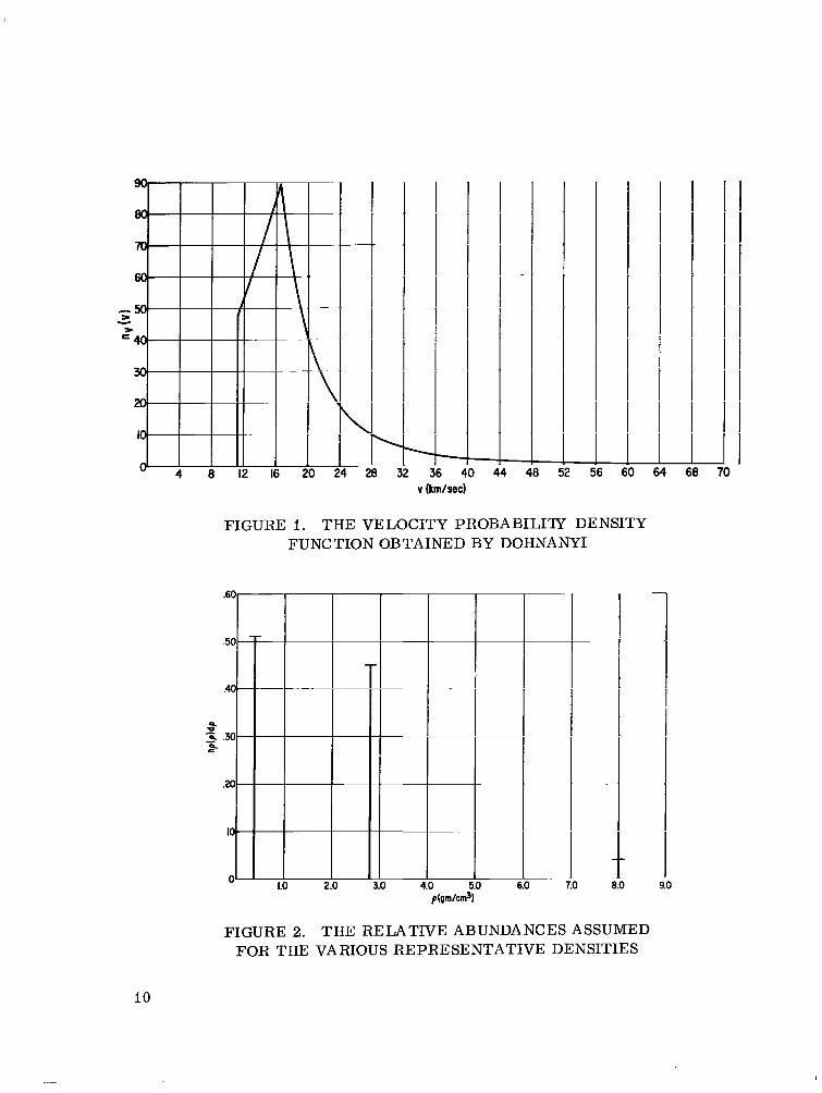
Dohnanyi [ I] applied this technique to a group of meteor observations by McCroskey and Posen and obtains a distribution function expressed by

c V I e 6 , 11.2 5 v 5 16.6 km/sec

C x I. 6 1 x I O 7 v-4-3 , 16.6 < v < 72.2 km/sec n (v) =

V

where C is the normalization constant. km/sec.

This distribution results in (v> = 19.17 Figure I shows this representation.

For lack of more definitive data o r contradictory evidence this dis- tribution will be assumed to apply to the entire mass spectrum of meteors.

The density distribution is more difficult to determine. Generally, the most definitive data available is the average density of a group of observations. Jacchia, Verniani and Briggs [ 2 j find an average p of 0.26 gm/cm3 for photo- graphic meteors. Verniani and Hawkins [ 31 for smaller masses find relative abundances between several groups of densities. Their tentative findings are 51 percent in a group less than I gm/cm3, with an average of 0.37 gm/cm3, 45 percent between I gm/cm3, with an average of 2.8 gm/cm3, and 4 percent greater than 12 gm/cm3. and probably result from small inaccuracies in the observed decelerations. the lack of more definitive data, the assumed density distribution will be taken as

The latter densities are of course unrealistically high, For

np ( p ) = 0. 5 1 x 0.37 6 ( p - 0.37) +

c 0 . 0 4 ~ 8 6 ( p - 8)

0.45 x 2.8 6 ( p - 2. 8)

(20)

where 6 ( p - p i ) are Dirac-Delta functions. assigned to the high density component reported by Verniani which represents the highest density which could be reasonably expected. Since the observables dealt with are fairly insensitive to density and density distribution, the inac- curacies in this distribution do not significantly affect the results. This choice of distribution gives ( p ) = I. 77 gm/cm3 which is somewhat higher than usually

The value of 8 was arbitrari ly

8

. . . . . -

b k

assumed. significant for the smaller particles.

This is due to the higher density contributions which may indeed be Figure 2 shows the assumed distribution.

OBSERVATIONAL DATA

Satellite Penetration Measurements

For determining the characterist ic mass for penetration of a given de- tector, the empirical Manned Space Center penetration formula has been utilized. This formula is usually written for semi-infinite targets in the nondimensional form

E = 1 . 64 d'/*'(cm) (pp/pT )*I2 (V COS e / c ) 2/3 d

where p is depth of penetration

d is equivalent projectile diameter

p is projectile density P

is target density PT

v is projectile velocity

c is target sound velocity

0 is the angle of incidence

The constant 1.64 applies to relatively hard (2024-T3) aluminum. It is more convenient to express this formula for aluminum in the form

9

I

v (km/sec)

- 52 !

I I I I I

I I 60 f

FIGURE I. THE VELOCITY PROBABILITY DENSITY FUNCTION OBTAINED BY DOHNANYI

FIGURE 2. THE RELATIVE ABUNDANCES ASSUMED FOR THE VARIOUS REPRESENTATIVE DENSITIES

10

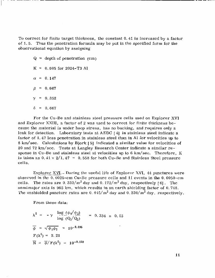
To correct for finite target thickness, the constant 0.41 is increased by a factor of I. 5. observational equation by assigning

Thus the penetration formula may be put in the specified form for the

Q = depth of penetration (cm)

K = 0.605 for 2024-T3 A1

a! = 0.147

Y = 0.352

6 = 0.667

For the Cu-Be and stainless steel p ressure cells used on Explorer XVI and Explorer XXIII, a factor of 2 was used to correct for finite thickness be- cause the material is under hoop s t r e s s , has no backing, and requires only a leak for detection. Laboratory tests at AEDC [ 41 in stainless steel indicate a factor of I . 47 less penetration in stainless steel than in A1 for velocities up to 8 km/sec. Calculations by Bjork [ 51 indicated a s imilar value for velocities of 20 and 72 km/sec. sponse in Cu-Be and stainless steel at velocities up to 6 km/sec. Therefore, K is taken as 0.41 x 2/1.47 = 0.558 for both Cu-Be and Stainless Steel p ressure cells.

Tests at Langley Research Center indicate a s imilar re-

Explorer XVI. - During the useful life of Explorer XVI, 44 punctures were observed-in the 0. 0025-cm Cu-Be pressure cel ls and I 1 events in the 0. 0050-cm cells. The rates are 0. 333/m2 day and 0. 172/m2 day, respectively [ 61 . The semimajor axis is 965 km, which resul ts in an ear th shielding factor of 0. 748. The unshielded puncture rates are 0. 445/m2 day and 0. 230/m2 day, respectively.

From these data:

- - 10-0.495 @ = 4@1@2 - F ( A o ) = 2. 21

Explorer XXIII- In one yea r Explorer XXIII observed 49 punctures of the 0.0025-cm stainless steel pressure cells and 74punctures in the 0.0050-cm cells. The rates are 0. 345/m2 day and 0. 205/m2 day, respectively [ 71 . The semimajor axis of the orbi t is 390 km, which resul ts in an ear th shielding factor of 0.674. Removing this results in puncture rates of 0. 526/m2 day and 0. 305/m2 day.

From these data:

ho = 0.278 f 0.11

F(ho) = 2.32

Pegasus. - Since the three Pegasus satellites had s imilar orbits, their data were combined. A s of January 1 , 1966, the 0.0038-cm detectors had counted 582 events for a rate of 0. 188/m2 day; the 0: 02-cm detectors had counted 49 events for a rate of 0. 021/m2 day; and the 0. 04-cm detectors had counted 201 events for a rate of 0. 00487/m2 day. shielded rates are 0.273, 0.0305, and 0. 00706/m2 day, respectively. aluminum thicknesses quoted are front sheets of parallel plate capacitors which are temporarily shorted by meteoroid penetration. In addition, a 0. 0012-cm mylar dielectric must also be penetrated. equivalent thickness of A1 is not yet known, but since i t is thin compared with the 0.02 and 0. 04 plate, no correction is applied to these thicknesses. mylar is a significant fraction of the 0. 0038-cm detector and must be considered in this case. 2024-T3, and is backed with a 0. 013-cm hard epoxy layer ra ther than soft foam. An effective thickness in t e r m s of the 0.02- and 0. 04-cm detectors has not yet been accurately determined; therefore, this datum point will not be used to determine the slope of the penetration curve. From the 0. 02-cm and 0. 04-cm points,

The shielding factor is 0.69. The un- The

The effect of this mylar in t e r m s of

The

Also, the 0. 0038-cm detect& is 1100-0 aluminum rather than

ho = 0.740 f 0.14

I. Clifton, K. S. and Naumann, R. J. : Pegasus Satellite Measurement of Meteoroid Penetration. NASA TM X ( in publication).

12

F ( A o ) = 1.76

- N = 10-2.076

Radar Observations

Elford [ 81 using a transmitted power of 1. 2 megawatts, reported a total

Reducing the transmitted power by a factor of 143 resulted in a flux of 9. 05 x 10-*/m2 day of meteors whose maximum line densities exceed 3.3 x 10" e/m. decrease in observed echoes by afactor of 12. Assuming the reflected electric field vector is proportional to the average trail density, the transmitted power required for a given reflected power varies as the inverse square of the electron line density. operation is 3. 94 x loi1 e/m.

Thus, the minimum detectable line density for the low power

Using the ionization efficiency determined by Verniani [ 91 , the maximum line density (e/m) may be related to mass by

(23) l o g q = 10.638 + log m + 4 l o g v + cos 8

where v is in km/sec and m is in grams.

The observational equation may be specified by setting

Q = electron line density, q (e /m)

log k = 10.638

a! = o

p = 4

Y = l

The ear th shielding factor is unity since the area in question is parallel to and facing away from the earth.

13

The first approximations are

A' = I. 005 f ?

5 = 10-3.583

F ( A o ) = 5. 94

- N = 10-4.358

Photographic Observations

Hawkins and Upton [ IO] determined the influx rate of photographic meteors in the range of -2. 5 to +3 photographic magnitude. expressed in t e rms of peak photographic magnitude Mp o r brighter as

Their observed flux may be

log @ = 0.537 Mp - 8.95 (no./m2 day) . (24)

The uncertainty in this relation is least from -2. 0 5 Mp 5 2. 5.

Jacchia, Verniani, and Briggs [ 31 performed a detailed analysis of a selected group of Super-Schmidt meteors whose masses were determined by integration of the total light curve. They found by method of least-squares a relation for peak brightness given by

Mp = 11.59 - 8.75 log v - 2.25 log m - I. 5 log 8 . (25)

log Q = Mp

log K = 11.59

c r = o

/3 = -8.75

y = -2. 25

6 = -1.5

14

I

From these data

A0 = 1.205 f 0. 06

F(ho) = 10.41

COMPUTATION PROCEDURE

The correction factor F ( A ) which relates observed number to cumulative directional flux depends on the measurement involved. Figure 3 for penetration, radar , and photographic measurements. concerning the interpretation of this factor may be in order . tains K which, when multiplied by the number per steradian, gives the total number incident on a flat surface. F ( h ) is less than K means that most of the observed punctures a r e caused by meteoroids with mass greater than the characterist ic mass. because of the reduced penetrating ability of particles impacting obliquely. the radar and photographic observations, the large velocity dependence allows a significant number of the more numerous meteors with masses smaller than m but with velocities higher than average to be observed; hence, the value of

F ( h ) is greater than K .

This factor is shown in A few comments

The factor con-

For penetration observations, the fact that

This is primarily For

C

The f i rs t approximations for h versus y = -log N are shown in Figure 4. Successive approximations may be obtained by the following process. log of equation (15) and differentiating,

Taking the

d log N d log F ( h ) d h d log N d l o g N = d l o g @ - d h

Let x = log m, y = -log N

15

14-

I 3 -

12- - x, I I - LL

IO

9 -

8 -

7 -

6 -

5 -

4 -

-

1.7

1.6

1.5-

NETRATION

- -

2.2 1 1 1 1 1 1 1 , , 1 I I I I

0 FIRST APPROXIMATION

V ITERATED VALUE (FIT I) A ITERATED VALUE ( F I T I I )

I .9

-I 1.4 I- 1.3 - 1.2 -

x 1.1 - 1.0 - .9 - .8 - .7 - .6 - .5 - .4 - .3

.2 - . I

-

- 0 I 2 3 4 5 6 7 8 9 1 0 1 1 1 2 1 3 1 4 I 5 I

y = -Log n (No./m2 day)

FIGURE 3. THE RATIO F(A) OF THE OBSERVED FLUX OF METEOROIDS TO THE NUMBER ENCOUNTERED PER

UNIT AREA TIME-SOLID-ANGLE WITH MASS SUF- FICIENT TO PRODUCE A THRESHOLD OBSERVATION

VELOCITY, AND NORMAL INCIDENCE

FIGURE 4. THE POSSIBLE FITS TO A AS A FUNCTION OF Y. THE DEPARTURES OF THE ITERATED VALUES OF FIT I FROM THE OB-

RECTIONS IN A INVOLVING dA/dy PROVIDED THEY HAVE AVERAGE DENSITY, AVERAGE SERVED VALUES ARISE FROM THE COR-

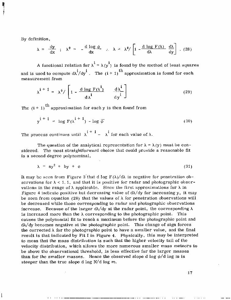
By definition,

i i A functional relation for A = h ( y ) is found by the method of least

i i th and is used to compute dh /dy . measurement from

The ( i + I) approximation is found for each

The (i + I) th approximation for each y is then found from

i + i Y

(28)

squares

i + 1 i The process continues until h = h for each value of A .

The question of the analytical representation for h = h ( y ) must be con- The most straightforward choice that could provide a reasonable f i t sidered.

is a second degree polynominal,

h = ay2 + by + c (31)

It may be seen from Figure S‘that d log F ( h ) / d X is negative for penetration ob- servations for h < i. i , and that i t is positive for radar and photographic obser- vations in the range of h applicable. Figure 4 indicate positive but decreasing value of dh/dy for increasing y , it may be seen from equation (28) that the values of h for penetration observations will be decreased while those corresponding to radar and photographic observations increase. Because of the larger dA/dy at the r ada r point, the corresponding h is increased more than the h corresponding to the photographic point. causes the polynomial f i t to reach a maximum before the photographic point and dA/dy becomes negative at the photographic point. the corrected h for the photographic point to have a smaller value, and the final resul t is that indicated by Fit I in Figure 4. Physically, this may be interpreted to mean that the mass distribution is such that the higher velocity tail of the velocity distribution, which allows the more numerous smaller mass meteors to be above the observational threshold, is less effective for the larger masses than for the smaller masses. steeper than the t rue slope d log N/d log m.

Since the f i r s t approximations for h in

This

This change of sign forces

Hence the observed slope d log @/d log m is

17

I

There is, of course, no theoretical justification in the choice of the The peak in A between the radar and polynomial chosen to represent A (y) .

photographic data may not correspond to physical reality. alternative representation was chosen that conditions A(y) to be monotonic, i. e. ,

For this reason, an

b - a + - 1 _ - A Y - C

The resul ts of this choice a r e indicated as Fit I in Figure 4. be considerable difference in the two resul ts , which more o r less represent extremes in the possible choices for A (y) , results, such as finding a mass distribution o r penetration frequency, are not seriously influenced by the choice of representation of A (y) .

There appears to

Fortunately, however, the end

The cumulative mass distribution may be found to within a constant of integration by solving the differential equation

or

l o g m = + d A ( Y )

For Fit I,

-2 log m = JiTTz I

where from the fit of A = A (y)

a = -0. 0328156

b = 0.425222

c = -0.550693

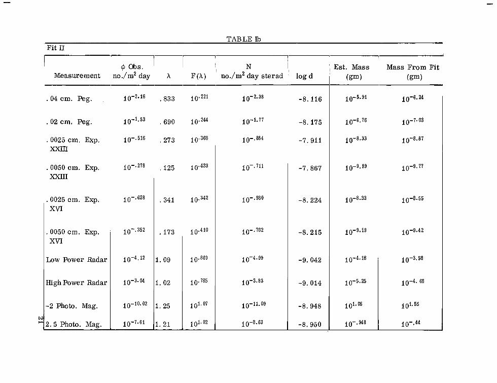
For Fit 11,

11 log M = - a log N - b In (-log N-c) + d

(34)

(35)

18

I1 where a, b, c have been determined from the fit of h = h (y)

a = 0.719683

b = 0.858195

c = 0.590827

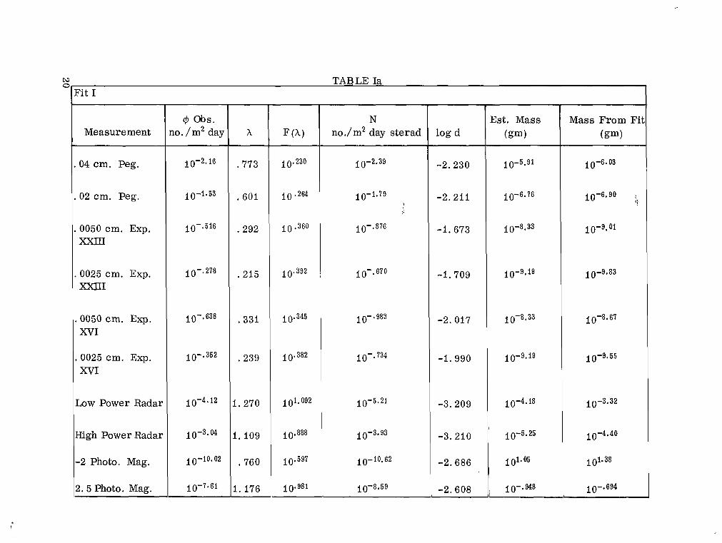
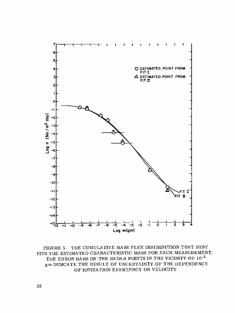
A value for d was computed for each datum point. Table I is a summary of these results. The average value and RMS deviation in d is -2.35 f 0.53 for Fit I and -8.45 f 0.46 for Fit 11, with the radar points producing the largest deviations in both cases. distribution is shown in Figure 5. slightly to the right of the mass distribution and photographic points fall slightly to the left. than predicted from the MSC formula o r that the masses inferred from photo- graphic data are too small. The radar points fall considerably on the small side. However, the uncertainty of + 0 .3 in the velocity exponent of the radar observational equation estimated by Verniani [ 31 is sufficient to bring these points into agreement.

Using the average value for d, the cumulative mass It may be seen that the satellite points fall

This means that meteoroids are either somewhat more penetrating

It is not necessary to actually use the mass estimates with their inherent uncertainties to obtain an expression for penetration frequency. Since penetration

Y P - m ,

log p = y log m + constant

log p = -1.6897 tanh-l [ 0.1575

for Fit I, o r for Fit 11,

log p = -0.2533 log N - 0.3021

(37)

(38)

og N + I. 02061 + d:: (39) I

n (-log N - 0. 5910) + d:: (40) 11

The constant d:: now contains the combination of material velocity, and

This constant can be determined for a particular material density te rms in the penetration formula as well as the constant of integration in the mass distribution. from a single penetration measurement. point,

Using the Pegasus 0. 04-cm datum

d:k = -0. 1054 I

19

N T A R T l i ’ To c

t I

~

‘it I

Measurement

04 cm. Peg.

02 cm. Peg.

0050 cm. Exp. XXTLT.

0025 cm. Exp. XXIII

0050 cm. Exp. XVI

0025 cm. Exp. XVI

x)w Power Radar

Iigh Power Radar

,2 Photo. Mag.

I. 5 Photo. Mag.

C#I Obs. io. /m2 day h

.773

.601

.292

.215

,331

.239

1.270

1. 109

.760

1.176

N no./m2 day sterad log d

-2.230

-2.211

-I. 673

-1.709

-2.017

-1.990

-3.209

-3.210

-2.686

-2.608

Est. Mass (gm)

Mass From Fil (gm)

Fit 11

I Measurement

. 04cm. Peg.

.02 cm. Peg.

.0025 cm. Exp. XXIII

.0050 cm. Exp. XXIII

.0025 cm. Exp. XVI

,0050 cm. Exp. XVI

Low Power Radar

High Power Radar

-2 Photo. Mag.

2.5 Photo. Mag.

1l-P' 1 @ Obs. I N I ', Est. Mass Mass From Fit I

t (gm) (gm) no./m2 day A F(A) no./m2 day sterad log d

.833

.690

,273

. 125

. 341

. I73

1. 09

1. 02

1. 25

1. 2 1

-8.116

-8.175

-7.911

-7.867

-8.224

-8.215

-9.042

-9.014

-8.948

-8.950

7 I I I I I 1 ~ 1 1 1 1 1 1 1 1 -

6 -

5 -

4 - 0 ESTIMATED POINT FROM - 3- A ESTIMATED POINT FROM - 2-

I -

0-

- -

FIT I

FIT It - - -

FIGURE 5. THE CUMULATIVE MASS FLUX DISTRIBUTION THAT BEST FITS THE ESTIMATED CHARACTERISTIC MASS FOR EACH MEASUREMENT.

THE ERROR BARS ON THE RADAR POINTS IN THE VICINITY OF IO-^ gm INDICATE THE RESULT OF UNCERTAINTY O F THE DEPENDENCE

O F IONIZATION EFFICIENCY ON VELOCITY

-I

0 -2- c )r

-0 (u E -3- >

c - 5 -

-4- U

3 -6-

-7

-8

-9

-10

-I I

-12

-13

-14

22

- - - - - - -

- - - - - - - - - - - -

L L I I 4 3 3 - 2 -I A ; ; ; 4

PENETRATION FREQUENCY

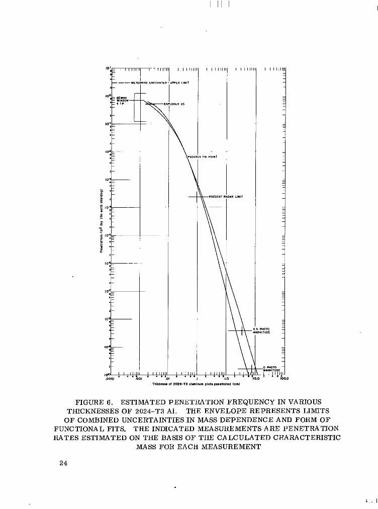
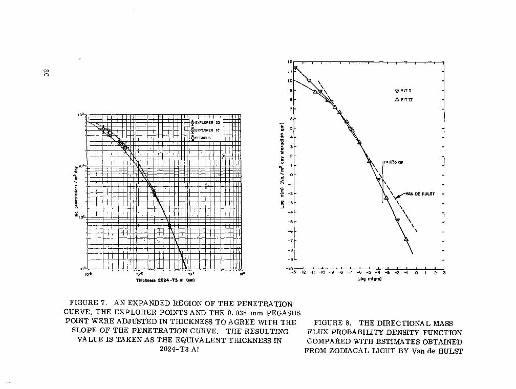
Figure 6 is a plot of the estimated frequency of penetration versus thick- ness of 2024-T3 A1 backed with foam. These same curves may be used for any other material by establishing an equivalent thickness of 2024-T3 for the material by laboratory impact tests. The maximum difference between Fit I and I1 is a factor of 0.4-in. thickness re- quired to give a certain penetration frequency. It is recommended that the largest value be used in all cases for a conservative design value. Table II is a summary of penetration frequency for various thickness of 2024-T3 A l .

The pessimistic curve resul ts from Fit II.

The other possible source of uncertainty in the penetration formula lies in the values of y used in obtaining the log derivatives. values of y = 0. 352 for penetration calculations and y = -2. 25 were used for photographic analysis. theoretical counterparts of 0. 333 and -2. 5.

Recall that empirical

These are slightly different from their respective

To investigate the possible effects of this uncertainty, the calculations The optimistic curve resul ts from Fit I with were also run with these values.

the smaller values of y , i. e. , 0.333 and -2.5. uncertainty, i. e. , the choice of analytical representation and the mass exponents have been analyzed with more or less extreme cases , the envelope of the re- sulting penetration curves may be considered to represent the limits with which penetrating flux can be predicted with available data. with increasing thickness, the spread is only a factor of 2 in thickness for the largest thickness of interest. have virtually no effect on this result .

Since the two major sources of

Although the limits diverge

Other choices of velocity o r density distributions

For thicknesses less than 0. 04 cm, the difference between the various cases is less . material equivalence between the 0. 0038-cm Pegasus point, the Explorer XVI points, and the Explorer XXUI points is avoided by the fact that the technique uses the slopes and the number observed rather than the actual thickness. for material equivalence can be inferred from this plot by taking the thickness in 2024-T3 A1 from the plot that corresponds to the observed penetration frequency. The resul ts are:

Figure 7 is an expanded plot of this region. The problem of

Values

23

... . .. .. . . . .. -. I

l l l l l

I I 1 1 1 1 1 1

WER LIMIT

IO I

--YETI

loo GEMINI

I I I I I I

,0001

IRER 23

PRESENT

\\

I I I l l 1 I I I I I l l I . s! I . . I

I I 1 1 1 1

I R LIMIT

PHOTO YlTUDE

1 0 PHOTO MAGNITUDE

- I 1 4 l!l!l ~~

100.0 Thickm.. of 2024-T3 dumlnum plat. panatrotad (em1

FIGURE 6. ESTIMATED PENETRATION FREQUENCY IN VARIOUS THICKNESSES O F 2024-T3 Al . THE ENVELOPE REPRESENTS LIMITS

O F COMBINED UNCERTAINTIES IN MASS DEPENDENCE AND FORM O F FUNCTIONAL FITS. THE INDICATED MEASUREMENTS ARE PENETRATION RATES ESTIMATED ON THE BASIS OF THE CALCULATED CHARACTERISTIC

MASS FOR EACH MEASUREMENT

24

Thickness 2024-T3 Plate (cm)

.003

.004

.005

. 006

. 007

. 008

.009

. 010

.020

.030

. 040

.050

. 060

. 070

.080

.090

.IO0

.200

TABLE 11

Upper Limit no. /m2 day

4.40 x I O - i

3.52 x IO”

2.81 x I O m i

2.31 x IO-i

I. 92 x IO-‘

I. 63 x IOm1

I. 49 x 10-1

I. 19 x 10-1

3.35 x

I. 39 x

7. IO x 10-3

4.30 x IO-^

2.50 x IO-^

I. 77 x IO-^

I . 28 x

8.50 x

6. 50 x

8.50 x

Lower Limit no. /m2 day

3.60 x IO-’

2.72 x 10-l

2.15 x IO-‘

I. 70 x IO-’

I. 40 x IO-’

I. 19 x 10-1

I . 01 x 10-1

8.90 x IO-’

2 . 9 0 x

I . 28 x

7. IO x IO-^

4.30 x 1 0 - ~

2.36 x

I. 60 x 10-~

1 . 1 0 ~ 10-~

7.40 x IO-^

5.40 x

5.60 x IO-^

25

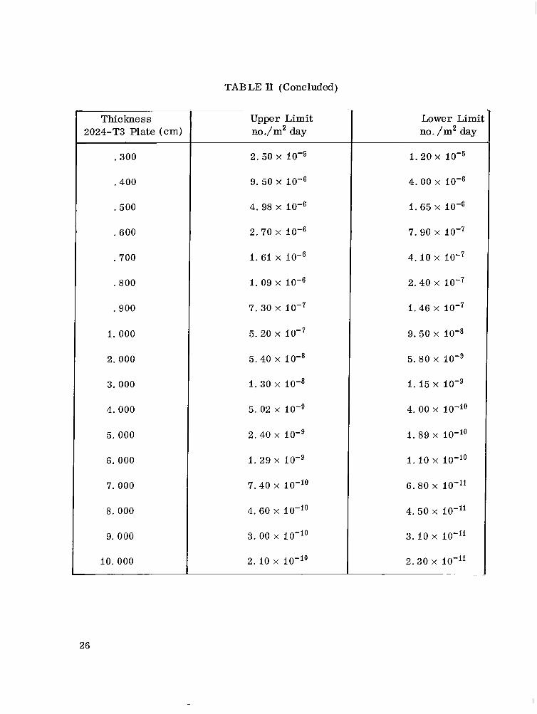
TAB LE II (Concluded)

Thickness 2024-T3 Plate (cm)

.300

.400

.500

.600

.700

.800

. g o o

I. 000

2.000

3.000

4.000

5.000

6.000

7.000

8.000

9.000

10.000

Upper Limit no./m2 day

2.50 x IO-^

9. 50 x

4. 98 x

2.70 x

I. 61 x

I. 09 x 10-6

7. 30 x IO-?

5.20 x IO-?

5.40 x

I. 30 x

5. 02 x

2.40 x

I. 29 x IO-^

7.40 x

4. 60 x I O - "

3.00 x io-'O

2.10 x

1 Lower Limit no. /m2 day

1 . 2 0 ~ IO-^

4 . 0 0 x

I. 65 x

7.90 x IO-?

4. IO x IO-?

2.40 x IO-?

I. 46 x IO-'

9.50 x

5.80 x

I. 15 x IO-^

4. 00 x 10-'O

I. 89 x I O - "

I. 10 x 10-'O

6. 80 x I O - "

4.50 x IO-' '

3.10 x 10-li

2.30 x I O - " ~

26

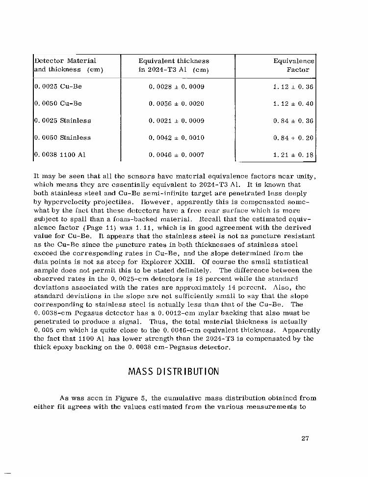
Detector Material and thickness (cm)

0. 0025 Cu-Be

0.0050 Cu-Be

0. 0025 Stainless

0. 0050 Stainless

0.0038 I100 A1

Equivalent thickness in 2024-T3 A1 (cm)

0.0028 f 0. 0009

0.0056 f 0. 0020

0.0021 f 0.0009

0. 0042 f 0. 0010

0.0046 f 0. 0007

Equivalence Factor

I . 12 f 0.36

I. 12 f 0.40

0.84 f 0. 36

0.84 f 0.20

1.21 f 0.18

It may be seen that all the sensors have material equivalence factors near unity, which means they are essentially equivalent to 2024-T3 A l . both stainless steel and Cu-Be semi-infinite target are penetrated less deeply by hypervelocity projectiles. However, apparently this is compensated some- what by the fact that these detectors have a free rear surface which is more subject to spa11 than a foam-backed material. Recall that the estimated equiv- alence factor (Page 11) was I. 11, which is in good agreement with the derived value for Cu-Be. as the Cu-Be since the puncture rates in both thicknesses of stainless steel exceed the corresponding rates in Cu-Be, and the slope determined from the data points is not as steep for Explorer XXIII. sample does not permit this to be stated definitely. observed rates in the 0. 0025-cm detectors is 18 percent while the standard deviations associated with the rates are approximately 14 percent. standard deviations in the slope are not sufficiently small to say that the slope corresponding to stainless steel is actually less than that of the Cu-Be. 0. 0038-cm Pegasus detector has a 0.0012-cm mylar backing that also must be penetrated to produce a signal. Thus, the total material thickness is actually 0. 005 cm which is quite close to the 0. 0046-cm equivalent thickness. the fact that 1100 A1 has lower strength than the 2024-T3 is compensated by the thick epoxy backing on the 0. 0038 cm-Pegasus detector.

It is known that

It appears that the stainless steel is not as puncture resistant

Of course the small statistical The difference between the

Also, the

The

Apparently

MASS D I STR I BUT I ON

A s was seen in Figure 5, the cumulative mass distribution obtained from either fi t agrees with the values estimated from the various measurements to

27

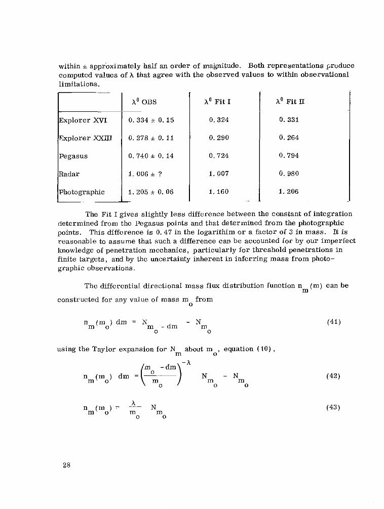
within f approximately half an order of magnitude. Both representations Eroduce computed values of A that agree with the observed values to within observational

c

Explorer XVI

Explorer Z I I I

Pegasus

Radar

Photographic

A' OBS

0.334 f 0.15

0.278 f 0.11

0.740 f 0.14

I. 006 f ?

I. 205 f 0.06 ~ ~

A' Fit I

0.324

0.290

0.724

I. 007

I. 160

A' Fit II

0.331

0.264

0.794

0. 980

I. 206

The Fit I gives slightly l e s s difference between the constant of integration determined from the Pegasus points and that determined from the photographic points. This difference is 0.47 in the logarithim o r a factor of 3 in mass. reasonable to assume that such a difference can be accounted for by our imperfect knowledge of penetration mechanics , particularly for threshold penetrations in finite targets, and by the uncertainty inherent i n inferring mass from photo- graphic observations.

It is

The differential directional mass flux distribution function n (m) can be m

constructed for any value of mass m from 0

n (m,) dm = N - N m m - d m m 0 0

using the Taylor expansion for N about m , equation (IO) , m 0

m ' N m m

0 ( m o ) = -

0

28

(42)

(43)

The resultant mass distribution is shown in Figure 8. It is interesting to compare this derived mass distribution with that of Van de Hulst [ 111 obtained from interpretation of the F-component of the solar corona and zodiacal light in t e rms of light diffracted from dust particles in interplanetary space. Hulst finds the photometric data can be well represented by a distribution in radii by

Van de

N ( a ) = c (no./cm3) (44 1

where

at I A. U. at 0 .5 A. U. < 0. I A. U.

for a < 0. 035 cm.

Taking the average density as I. 7 gm/cm3 and the average velocity as 20 km/sec, this distribution can be transformed to a distribution in directional mass flux encountered by an object in an orbit s imilar to that of the ear th ,

n (m) = I. 25 x (No./m2 day str. gm) . m

. It may be seen from Figure 6 that the agreement both in magnitude and

Van de Hulst s ta tes that particles with radii < 0. 035 cm are less slope between the mass distributions is remarkable for masses from gm to

gm. abundant than indicated by his distribution function, which agrees very well with present result.

A flattening and possible eventual decline of the distribution function for smaller masses would be expected as the result of the increased significance of radiation perturbations such as Poynting-Robertson effect and radiation pres- sure. The derived expressions for N approach a maximum value for the incident number which is 0. 738/m2 day steradian for Fit I and 0. 255/m2 day steradian for Fit II. The existing data do not extend to small enough masses to determine this accurately, but it is reasonably certain that only approximately 2-3 en- counters /m2 day can be expected with all meteoroids regardless of their mass. This is consistent with the fact that only one encounter in I. 4/m2 day exposure has been observed on Gemini windows' which sets a 90 percent upper limit of 2. 8/m2 day on events that produce discernable damage to optical surfaces.

I. Burbank, P. : Manned Space Center, private.communication, 1966.

It is

29

w 0

IC-3 IO+ IO' Thlcknm 2024-13 ol Icm)

-9 - -10 " " " " " " ' ~ ~

-13 -12 -I( -10 -9 -8 -7 -6 -5 -4 -3 -2 -1 0 I 2 3 Log m(gm)

FIGURE 7. AN EXPANDED REGION O F THE PENETRATION CURVE. THE EXPLORER POINTS AND THE 0.038 mm PEGASUS POINT WERE ADJUSTED IN THICKNESS TO AGREE WITH THE

VALUE IS TAKEN AS THE EQUIVALENT THICKNESS IN 2024-T3 A1

FIGURE 8. THE DIRECTIONAL MASS FLUX PROBABILITY DENSITY FUNCTION COMPARED WITH ESTIMATES OBTAINED

FROM ZODIACAL LIGHT BY Van de HULST

SLOPE OF THE PENETRATION CURVE. THE RESULTING

also interesting to note that meteoroid measurements from Mariner IV [ 121 from I - I. 56 A . U. observe between 0.63 and 2 . 8 events/m2 day.

No value for cut-off mass due to radiation pressure i f one indeed existsi can be inferred from the functions derived from either Fit I or 11 because the mass corresponding to the maximum N is 0.

(m) d m from the particles smaller than IOei3 gm is negligible. m a s s influx may be found by integrating

m The total

The mass contribution m n

m

m = s s c o s 6 dS2 s m n (m) dm m 2n 0 (45)

m AN

m m Since n (m) = -

m = ~ ! h N d m . m 0

T

For a small interval (mi , m2) the contribution in mass influx is found approx- imately using the Taylor expansion for N about mi m

The total mass influx is found by summing the incremental contributions. This presents no problem for Fit I1 since h approaches an asymptotic value greater than unity. However, using Fit I, h approaches 0 for masses greater than those corresponding to the photographic data. This leads to an infinite mass influx if the integration is carr ied to m = 0 0 . Since such masses exceed the limits of the data, there is no justification for extending the derivedexpression - - - -~

I. Often this limit is estimated by equating gravitational force to radiation pressure applied to the geometrical c ros s section of a sphere and solving for the radius. dimensions a r e of the order of or less than a visible wavelength. Shapiro showed that submicron metallic andall s izesof Si02 particles never have radiation pressure forces greater than gravitational forces.

This does not hold for dielectric particles or particles whose In fact

31

for N m datum point. be insignificant because of the rapidly decreasing population. the value for A for masses greater than 10 gm is I. 2, the contribution from larger masses is only 3 percent of the total.

into this region. Therefore the summation is car r ied only to the last The mass influx contributions for larger masses are believed to

If, for example ,

The total mass influx is found by 2 . 7 x lo-? gm/m2 day for Fit I and 1 . 4 x I O - ? gm/m2 day for Fit 11. This leads to a mass accretion of around 100 metric tons per day. extrapolation of photographic meteors to smaller masses which ranged from I000 to 10 000 tons per day.

This is considerably less than ea r l i e r estimates based on

Having determined the mass distribution, there a r e several other quan- tities of interest that may be easily found. flux may be found from

The normal component of momentum

m m

mv = [ r d a cos O J d v v cos On (v) dm m n ( m ) m 0 V .2n 0

(.) 2

1 3 T mv = -

mv 2 0 . 3 dyne - sec/m2 day I

or a pressure of 2 x sure.

N/m2 which is lo5 times smaller than radiation pres-

The energy flux is

E = 4 x Joules/m2 day

which over the entire earth amounts to a power input of 200 megawatts.

COMPARISONS WITH OTHER EXPERIMENTS

It appears that satellite penetration measurements together with radar and photographic observations of meteors yield a consistent picture of the ear th 's

32

meteoroid environment. picture and the previously accepted meteoroid environment based on collection experiments and acoustical and photomultiplier sensing of impacts from very small meteoroids. This disagreement had been suspected for some time be- cause of the failure of various early experiments using wire grids or s imilar sensors that required physical damage to detect anywhere near the number of events predicted by the acoustical measurements. The low puncture rate ob- served by Explorer XVI confirmed this disparity.

There is considerable disagreement between this

A s an example of the order of magnitude of this discrepancy, the mass flux relation obtained by Alexander et a1 [ 131 from acoustic measurement of the momentum imparted to sounding boards is

log N = -17 - I. 7 log M

where N is the number of encounters pe r square meter second with meteoroids of mass M o r greater . The characterist ic mass for the Explorer XVI 0. 0025- cm pressure cells is 10-9.55 gm. From Alexander's results the cells should be punctured at a rate of 10-1.5 per m2 second o r per square meter day. This is almost four orders of magnitude higher than what was actually observed. Furthermore, the quantity d log N/d log M is -1.7 according to Alexander's re- sults but was observed to be only -0. 3 from the penetration measurements. is inconceivable that a measurement as straightforward as the Explorer XVI pressure cell experiment could measure four o rde r s of magnitude too low. of the cells eventually registered a puncture, which is convincing evidence that the cells retained pressure and therefore were not punctured pr ior to the indicated time. (I) the acoustical data are in serious e r r o r , o r (2 ) meteoroids are far less penetrating than expected. predict characterist ic mass for puncture is an extrapolation, it is based on laboratory data which contains the size range in question and velocities well in- to the meteoroid range ( > 10 km/sec). Most of the small mass , high velocity penetration data have been restricted to densities of I gm/cm3 and higher, but theoretical studies [ 51 indicate high velocity particles of porous A1 (0.44 gm/cm3) are just as penetrating for a given mass as those of normal density. acoustical measurements are actually measuring momentum of impacting mete- oroids, the only explanation of the failure to observe a large number of penetra- tions in very thin metallic foils must be a combination of very low relative ve- locities and extremely tenuous particles. orbits s imilar to the orbit of the satellite carrying the measurement, the fact that the satellites involved have fairly high inclinations requires the particles to have

It

Most

There appears to be only two possible explanations of this discrepancy;

Although the empirical penetration formula used to

If the

Even if such particles were in geocentric

33

relative velocities as high as 8 km/sec, with an average velocity of around 5 km/sec. XXIII pressure cel ls and the failure to observe any penetrations on Jennison's 143 0.0012- and 0. 0015-cm foils on A r i e l I1 require incredibly low densities. It is clear that to explain both the acoustic measurements and the penetration measurements, it is necessary to assume two distinct families of meteoroids. The mass distribution obtained in this work applies to moderate density, penetrating particles in heliocentric orbits. distribution is such that a very small fraction of the acoustic events can be attributed to this family. encounters, the particles must belong to a family of extremely tenuous, non- penetrating particles in a distribution whose population declines rapidly 'with increasing mass. The much smaller decrease in population with mass observed for the family of penetrating particles indicates that an insignificant fraction of observed penetrations can be attributed to the more massive members of the family of non-penetrating particles.

The low penetration rate observed on the 0. 0025-cm Explorer XVI and

The slope and magnitude of this

If the acoustic events are actually caused by meteoroid

The assumption of this near-earth dust belt whose mass distribution is approximately four o rde r s of magnitude higher than the interplanetary back- ground raises a major theoretical objection which has not been resolved despite considerable efforts on the par t of several investigators. s ize and apparent low density, such particles in a near-earth orbit could not remain indefinitely because of radiation perturbations. somehow be supplied. An extensive analysis of possible concentration mechanisms was performed in which no means of providing a concentration of dust in the vicinity of the ear th to the extent implied by the acoustic measurements was found.

Because of their small

Therefore , they must

The difficulties encountered in attempting to explain the existence of such a near-earth concentration of dust as well as the peculiar properties that must be ascribed to such dust particles to account for their failure to penetrate very thin metallic foils demand that the evidence for their existence be reevaluated. The bulk of this evidence has been supplied by acoustical measurements. recently been demonstrated that certain types of acoustical impact measuring devices are susceptible to noise during thermal cycling. '9 the fact that acoustical detectors operating in the vicinity of earth where they t raverse the ear th 's shadow exhibit a high count rate while the same detectors operating in a fairly constant thermal environment on space probes give results

1. Shapiro, I. I. ; Lautman, D.A. ; and Colombo, G. : The Earth's Dust Belt: Fact or Fiction. J. Geophys. Res. ( to be published).

2. Private discussions with personnel a t Langley Research Center, Sept. 1965.

3. Nilsson, C. : Some Doubts about the Earth's Dust Cloud. Science ( to be

It has

This could account for

-~

published).

34

reasonably consistent with estimates based on penetration experiments and zodiacal light studies. experiments flown on satellites as well as rocket probes have returned a very large number of particles, some of which were collected undamaged.

However, there is still the unexplained fact that collection

It is clear that there are still many unanswered questions that must be resolved before all of the above measurements can be properly interpreted. Since there is some doubt concerning the measurements that imply the large concentration of non-penetrating particles, these data are not used in the present analysis. If these measurements can be verified, and the existence of a near- ear th dust belt of extremely tenuous particles is demonstrated, the mass distri- bution obtained in this present analysis must be modified to include this com- ponent. particles must then be solved. It is not considered likely that such a finding will alter the penetration frequency predictions obtained by the present study for thicknesses greater than 0. 01 mm aluminum.

Several challenging problems concerning the origin and nature of such

CONCLUSIONS

A penetrating flux model has been developed by essentially extrapolating the Pegasus data to larger and smaller thickness using slopes d log N/d log M determined from ground based and other satellite penetration measurements. The major source of uncertainty lies in the functional relations of mass to penetration and of mass to peak photographic magnitude. A secondary source lies in the freedom of choices in the representation of these slopes as a function of cumulative flux. This freedom can be restricted substantially by additional r ada r o r photographic measurements of this log derivative from N = IO4 to I O 6 per m2 day steradian, i. e. , between Elford's data and the Super-Schmidt data. Such measurements can certainly be made and perhaps already exist, but have not been reported in a form amenable to this analysis. A s for the uncertainties in the mass relation, the problem a r i s e s because the empirical values for the mass exponent differ from those embodied in the theoretical models. some uncertainty exists until the reasons for these differences are understood.

Therefore,

A "best fit" cumulative mass flux has been found to within a constant of integration without having to specify the mass involved in any observation. A constant of integration was calculated for each measurement by estimating a value-for the mass (having average velocity, average density, and normal in- cidence) characteristic to the observation. used in the "best fit" mass flux.

The average of these constants was

35

The mass distribution function was obtained from the cumulative mass flux and is found to agree remarkably well with the interplanetary dust distri- bution derived by Van de Hulst from interpretation of photometric measurements of F-corona and zodiacal light. Also it was found that interplanetary measure- ments of dust by Alexander on Mariner IV were in order of magnitude agreement. These results suggest that the environment is not substantially different in interplanetary space. Also the fact that the slopes determined from satellite penetration data appear to rapidly approach zero as N increases , suggests an upper limit on the number of meteoroid encounters which appears to be on the order of 3/m2 day regardless of size. that only one discernable impact crater was found on a Gemini window. This also suggests that erosion from meteoroids is insignificant and that puncture rate in thin materials is f a r less than earlier estimates. This low value for the maximum encounter frequency demands that a meaningful meteoroid experiment must expose an area on the order of a m2 to collect a good statistical sample in a reasonable time.

This low value is consistent with the fact

There is a possibility that there exists, in addition to the family of meteoroids treated in this study, a very large population of particles concentrated near-earth that for some reason are not able to penetrate materials as thin as 0.01 mm aluminum. How such a concentration could exist and how the particles in this family could have such low penetrating power are not understood. Until the existence of this family is more conclusively demonstrated, it will not be con- sidered. Even if this family does exist, the low penetrating ability of its con- sistent particles must be such that it will not contribute significantly to the meteoroid hazard estimates presented in this paper.

36

REFER EN CE S

I. Dohnanyi, J. S. : Model Distribution of Photographic Meteors. Bellcomm TR-66-340-1, March 29, 1966.

2. Jacchia, L. G. ; Verniani, F. ; and Briggs, R. E. : Smithsonian Special Report No. 175, April 23, 1965.

3. Verniani, F. and Hawkins, G. S . : Masses, Magnitudes, and Densities Harvard Radio Meteor Project Research Report of 320 Radio Meteors.

No. 12, March 1965.

4. Payne, J. J. : Impacts of Spherical Projectiles of Aluminum, Stainless Steel, Titanium, and Lead into Semi-infinite Targets of Aluminum and Stainless Steel. AEDC-TR-65-34, Arnold A i r Force Station, Tennessee, February 1965.

5. Bjork, R. L. : Final Report. NASW-805 Shock Hydrodynamics, Inc. , Sherman Oaks, California, 1966.

6. D'Aiutolo, C. T. : Review of Meteoroid Environment Based on Results from Explorer XIII and Explorer XVI Satellites. Space Science Symposium of COSPAR, Warsaw, Poland, June 1963.

Fourth International

7. O'Neal, R. L. : NASA TM X-I123 August 1965.

8. Elford, W. G. : Calculation of the Response Function of the Harvard Radio Meteor Project Radar System. Radio Meteor Project Research Report No. 8, October 1964.

9. Verniani, F. ; and Hawkins, G. S . : On the Ionizing Efficiency of Meteors. Harvard Radio Meteor Project Research Repor t No. 5, February 1964.

I O . Hawkins, G. S . ; and Upton, E. K. L. : The Influx Rate of Meteors in the Earth 's Atmosphere. Astrophys. J. , Vol. 128, pp. '727-735, 1958.

11. Van de Hulst, H. C. : Zodiacal Light in the Solar Corona. Astrophys. J . , Vol. 105, pp. 471-488, 1947.

37

REFERENCES (Concluded)

12. Alexander, W. M. ; McCracken, C. W. ; and Bohn, J. L.: Zodiacal Dust: Measurements by Mariner IV. Science, Vol. 149, pp. 1240-1241, 1965.

13. McCracken, C. W. ; and Alexander, W. M. : Direct Measurements of Interplanetary Dust Particles in the Vicinity of Earth. December 1961.

NASA T N D-1174,

14. Jennison, R. C. ; and McDonnell, J. A. M. : Interpretation of the Inter- Presented at the

Cambridge, Mass., planetary Dust Measurements in the Ariel 11 Satellite. International Symposium on Meteor Orbits and Dust. August I 965.

38 M418 NASA-Langley, 1966

1

“The aeronazitical and space activities of the United States shall be conducted so as to contribvte . . . to the expansion of hzinian knowl- edge of phenomena in the atmosphere and space. T h e Administi,ation shall provide for the widest practicable and appropriaf e dissemination of information concerning its actirdies and the reszilts thereof.”

-NATIONAL AERONAUTICS A N D SPACE ACT OF 1958

NASA SCIENTIFIC A N D TECHNICAL PUBLICATIONS

TECHNICAL REPORTS: important, complete, and a lasting contribution to existing knowledge.

TECHNICAL NOTES: of importance as a contribution to existing knowledge.

TECHNICAL MEMORANDUMS: Information receiving limited distri- bution because of preliminary data, security classification, or other reasons.

CONTRACTOR REPORTS: Technical information generated in con- nection with a NASA contract or grant and released under NASA auspices.

TECHNICAL TRANSLATIONS: Information published in a foreign language considered to merit NASA distribution in English.

TECHNICAL REPRINTS: Information derived from NASA activities and initially published in the form of journal articles.

SPECIAL PUBLICATIONS: Information derived from or of value to NASA activities but not necessarily reporting the results of individual NASA-programmed scientific efforts. Publications include conference proceedings, monographs, data compilations, handbooks, sourcebooks, and special bibliographies.

Scientific and technical information considered

Information less broad in scope but nevertheless

Details on the availability o f these publications may be obtained from:

SCIENTIFIC AND TECHNICAL INFORMATION DIVISION

NATIONAL AERONAUTICS AND SPACE ADMINISTRATION

Washington, D.C. 20546