the multiple absorption coefficient zonal method …yuen/current_paper/zonal_nht.pdfwalter w. yuen...

1

The Multiple Absorption Coefficient Zonal Method (MACZM), an Efficient

Computational Approach Radiative Heat Transfer in Multi-Dimensional

Inhomogeneous Non-gray Media

Walter W. Yuen

Department of Mechanical and Environmental Engineering

University of California at Santa Barbara

Santa Barbara, California, 93105

ABSTRACT

The formulation of a multiple absorption coefficient zonal method (MACZM) is

presented. The concept of generic exchange factors (GEF) is introduced. Utilizing the GEF

concept, MACZM is shown to be effective in simulating accurately the physics of radiative

exchange in multi-dimensional inhomogeneous non-gray media. The method can be directly

applied to a fine-grid finite-difference or finite-element computation. It is thus suitable for

direction implementation in an existing CFD code for analysis of radiative heat transfer in

practical engineering systems.

The feasibility of the method is demonstrated by calculating the radiative exchange

between a high temperature (~3000 K) molten nuclear fuel (UO2) and water (with a large

variation in absorption coefficient from the visible to the infrared) in a highly 3-D and

inhomogeneous environment simulating the premixing phase of a steam explosion.

NOMENCLATURE a = absorption coefficient

A = area element

dA = differential area element

dV = differential volume element

D = length scale (grid size) of the discretization

2

ggzzF = dimensionless volume-volume exchange factor, Eq. (11a)

ggxzF = dimensionless volume-volume exchange factor, Eq. (11b)

gszF = dimensionless volume-surface exchange factor, Eq. (14a)

gsxF = dimensionless volume-surface exchange factor, Eq. (14b)

1 2g g = volume-volume exchange factor, Eq. (1)

1 2g s = volume-surface exchange factor, Eq. (5)

cL = characteristic lengths between two elements along the selected optical path

mbL = mean beam length between two volume (area) elements, Eq. (16)

n = unit normal vector

, ,x y zn n n = dimensionless distance coordinate, Eq. (12)

r = distance between volume elements, Eq. (3)

s = distance, Eq. (4)

1 2s s = surface-surface exchange factor, Eq. (6)

V = volume element

Q = heat transfer

T = temperature

x = coordinate

y = coordinate

z = coordinate

σ = Stefan Boltzmann constant

τ = optical thickness, Eq. (3)

subscripts

1,2 = label of volume (area) element

3

INTRODUCTION

The ability to assess the effect of radiation heat transfer in multi-dimensional

inhomogeneous media is important in many engineering applications such as the analysis of

practical combustion systems and the mixing of high temperature nuclear fuel (UO2) with water

in the safety consideration of nuclear reactors. The lack of a computationally efficient and

accurate approach, however, has been a major difficulty limiting engineers and designers from

addressing many of these important engineering issues accounting for the effect of thermal

radiation.

For example, in the analysis of steam explosion in a reactor safety consideration, it is important

for account for the radiative exchange between hot molten material (e.g. UO2) and water. The

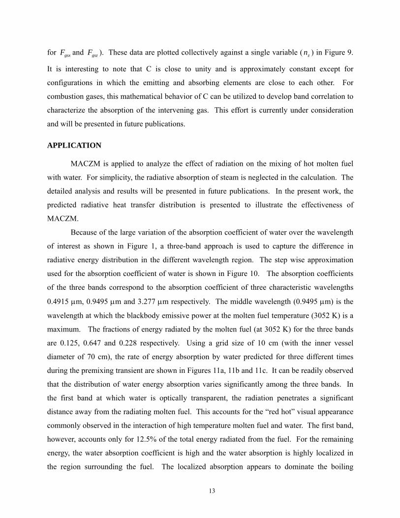
absorption coefficient for water is plotted together with the blackbody emissive power at 3052 K

(the expected temperature of molten UO2 in a nuclear accident scenario) in Figure 1. The

radiative exchange between water and UO2 must account for the highly nongray and rapidly

increasing (by more than two order of magnitude) characteristic of the absorption coefficient of

water. The multi-dimensional and inhomogeneous aspect of the “premixing” process are

illustrated by Figure 2. In this particular physical scenario, molten UO2 is released from the top

into a cylindrical vessel with an annular overflow chamber as shown in the figure. Even with

highly subcooled water (say, 20 C at 1 atm), voiding occurs quickly leading to a complex two

phase mixture surrounding the hot molten UO2. The radiative heat transfer between the hot

molten UO2 and the surrounding water is a key mechanism controlling the boiling process. The

boiling process, on the other hand, depends on the radiative heat transfer and thus the amount of

liquid water surrounding the hot molten material. An accurate assessment of this interaction is

key to the understanding of this “premixing” process and ultimately to the resolution of the

critical issue of steam explosion in the consideration of reactor safety.

Over the years, the zonal method has been shown to be an effective approach to account

for the multi-dimensional aspect of radiative heat transfer in homogeneous and isothermal media

[1]. This method was later extended for application to inhomogeneous and non-isothermal media

with the concept of “generic” exchange factors (GEF) [2]. The underlying principle of the

extended zonal method is that if a set of generic exchange factors with standard geometry is

tabulated, the radiative exchange between an emitting element and an absorbing element of

arbitrary geometry can be generated by superposition. The inhomogeneous nature can be

4

accounted for by using the appropriate average absorption coefficient in the evaluation of the

generic exchange factor. As grid size decreases, it is expected that the accuracy of the

superposition will increase, The error of using a single average absorption to account for the

absorption characteristics of the intervening medium will also decrease.

While the extended zonal method was effective in accounting for the effect of an

inhomogeneous medium in some problems [2], the accuracy of the approach for general

application is limited. Specifically, by using a set of GEF which depends on only a single

average absorption coefficient, the method do not simulate correctly the physics of radiative

exchange between two volume elements which depends generally on at least three characteristic

absorption coefficients (namely, the absorption coefficient of the emitting element, the

absorption coefficient of the absorbing element and the average absorption coefficient of the

intervening medium). A reduction in grid size cannot address this fundamental limitation.

In addition, the concept of a single average absorption coefficient for the intervening

medium is also insufficient, particularly in an environment where there is a large discontinuity of

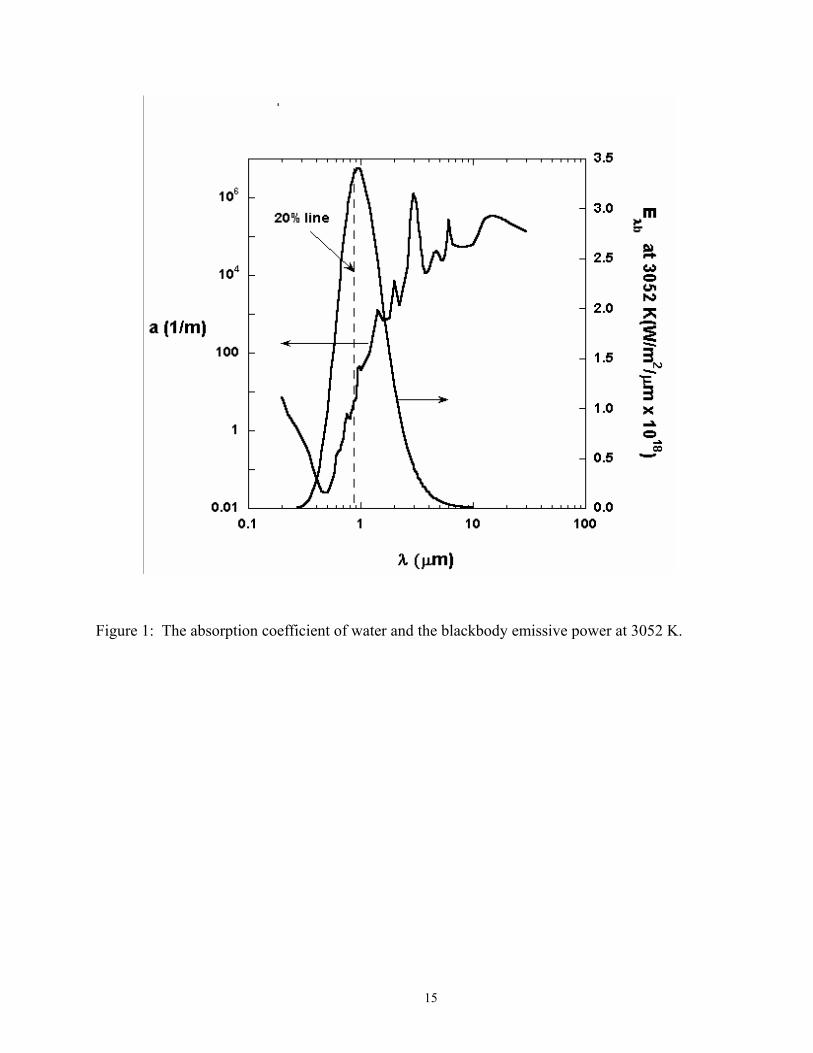
the absorption coefficient. For example, consider the radiative exchange between a radiating

cubical water element V1 and an absorbing cubical water element V2 as shown in Figure 3. The

absorbing element V2 is an element at the liquid/vapor phase boundary. It is adjacent to another

element of liquid water on one side while surrounded by a medium which is effectively optically

transparent. As shown in the same figure, there are two possible optical paths, indicated as S1

and S2, over which the average absorption coefficient can be evaluated. For the physical

dimensions as shown in the figure, the average absorption coefficient evaluated along the optical

path S2 increases from 6.38 1/cm to 306 1/cm as the wavelength increases from 0.95 µm to 3.27

µm while the average absorption coefficient evaluated along the optical path S1 remains

effectively at zero (ignoring the very small absorption by water vapor). It would be difficult to

evaluate the radiative exchange between these two elements accurately using a single exchange

factor based on a single average absorption coefficient for the intervening medium. This large

discrepancy in the average absorption coefficient of the two optical paths remains even in the

limit of small grid size.

The objective of the present work is to present the mathematical formulation of a

multiple absorption coefficient zonal method (MACZM) which is mathematically consistent

with the physics of radiative absorption. The method will be shown to be efficient and accurate

5

in the simulation of radiative heat transfer in inhomogeneous media. A set of “three absorption

coefficient” volume-volume exchange factors and “two absorption coefficient” volume-surface

exchange factors are tabulated for rectangular elements. The generic exchange factor (GEF)

concept is expanded to a two-component formulation to account for the possible large variation

of absorption coefficient in regions surrounding the absorbing or emitting elements. Based these

two-component generic exchange factors, the multi-dimensional and non-gray effect in any

discretized domain can be evaluated accurately and efficiently by superposition. The accuracy of

the superposition procedure is demonstrated by comparison with results generated by direct

numerical integration. The characteristics of radiative exchange in a highly multi-dimensional,

inhomogeneous and non-gray media such as those existed in the premixing phase of a steam

explosion (as shown in Figure 2) are presented to illustrate the feasibility of the approach.

MATHEMATICAL FORMULATION General Formulation

The basis of the zonal method [1] is the concept of exchange factor. Mathematically, the

exchange factor between two discrete volumes, 1V and 2V , in a radiating environment is

1 2

1 2 1 21 2 2

V V

a a e dV dVg gr

τ

π

−

= ∫ ∫ (1)

where

( ) ( ) ( )1/ 22 2 2

1 2 1 2 1 2r x x y y z z⎡ ⎤= − + − + −⎣ ⎦ (2)

τ is the optical thickness between the two differential volume elements, 1dV and 2dV , given by

6

( )2

1

r

r

a s dsτ = ∫ (3)

with a being the absorption coefficient and

1s r r= − (4)

The integration in Eq. (3) is performed along a straight line of sight from 1r to 2r .

In a similar manner, the exchange factor between a volume element 1V and a surface

element 2A and that between two area elements 1A and 2A are given, respectively, by

1 2

1 2 1 21 2 3

V A

a e n r dV dAg s

r

τ

π

− ⋅= ∫ ∫ (5)

1 2

1 2 1 21 2 4

A A

e n r n r dAdAs s

r

τ

π

− ⋅ ⋅= ∫ ∫ (6)

where 1n and 2n are unit normal vectors of area elements 1dA and 2dA .

It should be noted that Eqs. (1), (5) and (6) are applicable for general inhomogeneous

non-scattering media in which the absorption coefficient is a function of position. Physically,

the exchange factor can be interpreted as the fraction of energy radiated from one volume (or

area) and absorbed by a second volume (or area). Specifically, for a volume 1V with uniform

temperature 1T , the absorption by a second volume 2V of radiation emitted by 1V is given by

7

1 2

41 1 2V VQ T g gσ→ = (7)

and the absorption by a black surface 2A of radiation emitted by 1V is given by

1 2

41 1 2V AQ T g sσ→ = (8)

Similarly, for a black surface 1A with uniform temperature 1T , the absorption by a volume 2V of

radiation emitted by 1A is given by

1 2

41 1 2A VQ T s gσ→ = (9a)

where, by reciprocity,

1 2 2 1s g g s= (9b)

Finally, the absorption by a black surface 2A of radiation emitted by 1A is given by

1 2

41 1 2A AQ T s sσ→ = (10)

The Discretization

The evaluation of Eqs. (7) to (10) in a general transient calculation in which the spatial

distribution of the absorption coefficient is changing (for example, due to the change in the

8

spatial distribution of hot materials and void fraction during the “premixing” process as shown in

Figure 2) is too time consuming even with fast computers. Anticipating that all calculations will

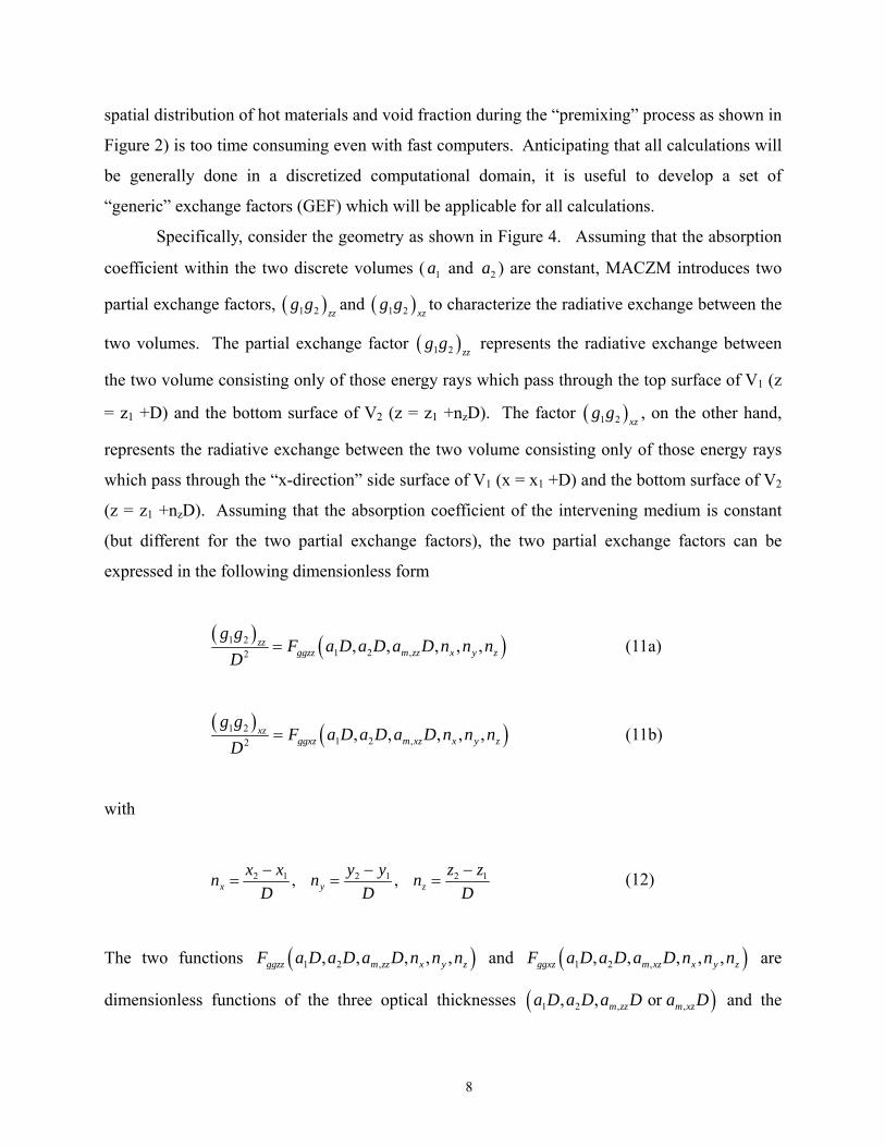
be generally done in a discretized computational domain, it is useful to develop a set of

“generic” exchange factors (GEF) which will be applicable for all calculations.

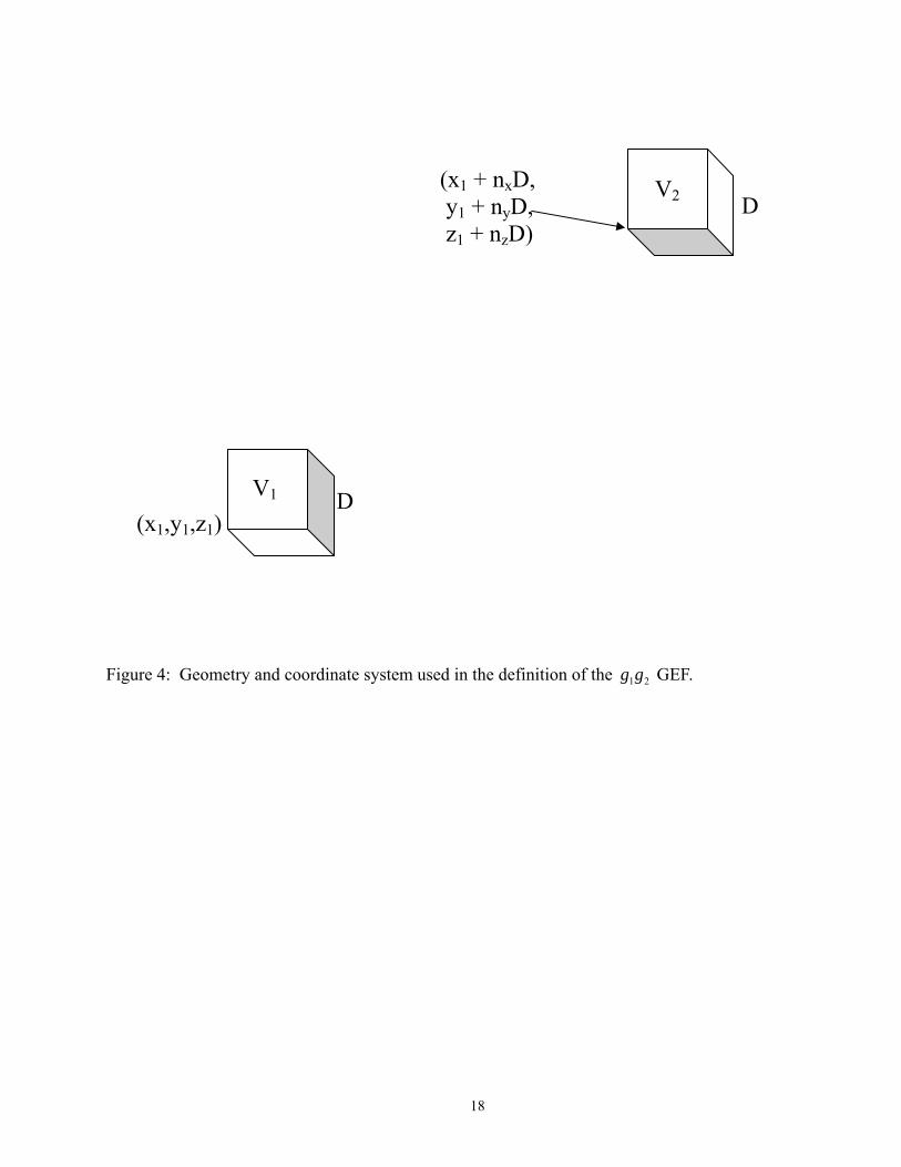
Specifically, consider the geometry as shown in Figure 4. Assuming that the absorption

coefficient within the two discrete volumes ( 1a and 2a ) are constant, MACZM introduces two

partial exchange factors, ( )1 2 zzg g and ( )1 2 xz

g g to characterize the radiative exchange between the

two volumes. The partial exchange factor ( )1 2 zzg g represents the radiative exchange between

the two volume consisting only of those energy rays which pass through the top surface of V1 (z

= z1 +D) and the bottom surface of V2 (z = z1 +nzD). The factor ( )1 2 xzg g , on the other hand,

represents the radiative exchange between the two volume consisting only of those energy rays

which pass through the “x-direction” side surface of V1 (x = x1 +D) and the bottom surface of V2

(z = z1 +nzD). Assuming that the absorption coefficient of the intervening medium is constant

(but different for the two partial exchange factors), the two partial exchange factors can be

expressed in the following dimensionless form

( ) ( )1 21 2 ,2 , , , , ,zz

ggzz m zz x y z

g gF a D a D a D n n n

D= (11a)

( ) ( )1 21 2 ,2 , , , , ,xz

ggxz m xz x y z

g gF a D a D a D n n n

D= (11b)

with

2 1 2 1 2 1, , x y zx x y y z zn n n

D D D− − −

= = = (12)

The two functions ( )1 2 ,, , , , ,ggzz m zz x y zF a D a D a D n n n and ( )1 2 ,, , , , ,ggxz m xz x y zF a D a D a D n n n are

dimensionless functions of the three optical thicknesses ( )1 2 , ,, , or m zz m xza D a D a D a D and the

9

dimensionless separation between the two volume elements ( ), ,x y zn n n . For a rectangular

discretization with constant grid size (dx = dy = dz = D), these dimensionless distances only take

on discretized value, i.e. , , 0,1,2x y zn n n = ⋅⋅ ⋅ . The two dimensionless function tabulated at

different optical thicknesses ( )1 2 , ,, , or m zz m xza D a D a D a D and discretized values of ( ), ,x y zn n n

constitutes two sets of “generic” exchange factor (GEF) which will be applicable for all

calculations with uniform grid size. The intervening absorption coefficient ma is the average of

the absorption coefficient taken along a line of sight directed from the center of the top area

element of V1 (z = z1 +D) to the center of the bottom surface of V2 (z = z1 +nzD). Similarly,

the intervening absorption coefficient ,m xza is the average of the absorption coefficient taken

along a line of sight directed from the center of the “x-direction” side area element of V1 (x = x1

+D) to the center of the bottom surface of V2 (z = z1 +nzD).

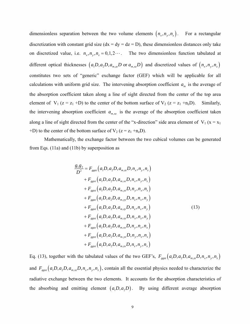
Mathematically, the exchange factor between the two cubical volumes can be generated

from Eqs. (11a) and (11b) by superposition as

( )( )( )( )( )

1 21 2 ,2

1 2 ,

1 2 ,

1 2 ,

1 2 ,

1 2

, , , , ,

, , , , ,

, , , , ,

, , , , ,

, , , , ,

, ,

ggzz m zz x y z

ggxz m xz x y z

ggxz m yz y x z

ggzz m yy z x y

ggxz m zy z x y

ggxz

g g F a D a D a D n n nD

F a D a D a D n n n

F a D a D a D n n n

F a D a D a D n n n

F a D a D a D n n n

F a D a D

=

+

+

+

+

+ ( )( )( )( )

,

1 2 ,

1 2 ,

1 2 ,

, , ,

, , , , ,

, , , , ,

, , , , ,

m xy x z y

ggzz m xx y z x

ggxz m yx y z x

ggxz m zx z y x

a D n n n

F a D a D a D n n n

F a D a D a D n n n

F a D a D a D n n n

+

+

+

(13)

Eq. (13), together with the tabulated values of the two GEF’s, ( )1 2 ,, , , , ,ggzz m zz x y zF a D a D a D n n n

and ( )1 2 ,, , , , ,ggxz m xz x y zF a D a D a D n n n , contain all the essential physics needed to characterize the

radiative exchange between the two elements. It accounts for the absorption characteristics of

the absorbing and emitting element ( )1 2,a D a D . By using different average absorption

10

coefficients ( ), , , , ,m pqa D p q x y z= for the intervening medium, it accounts for not only the

absorption characteristics of the intervening medium, but also and the variation of absorption

characteristics in the neighborhood of the absorbing and emitting elements (such as the situation

as shown in Figure 3).

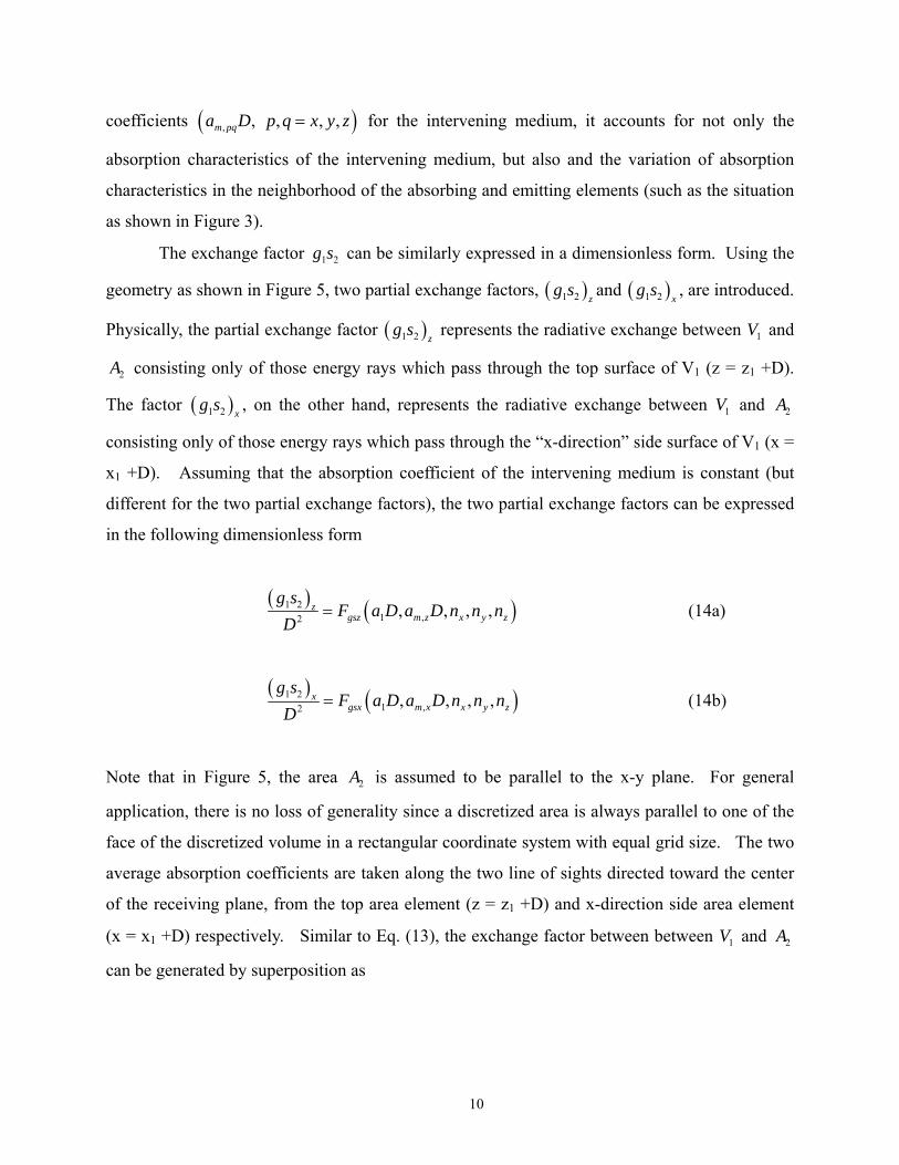
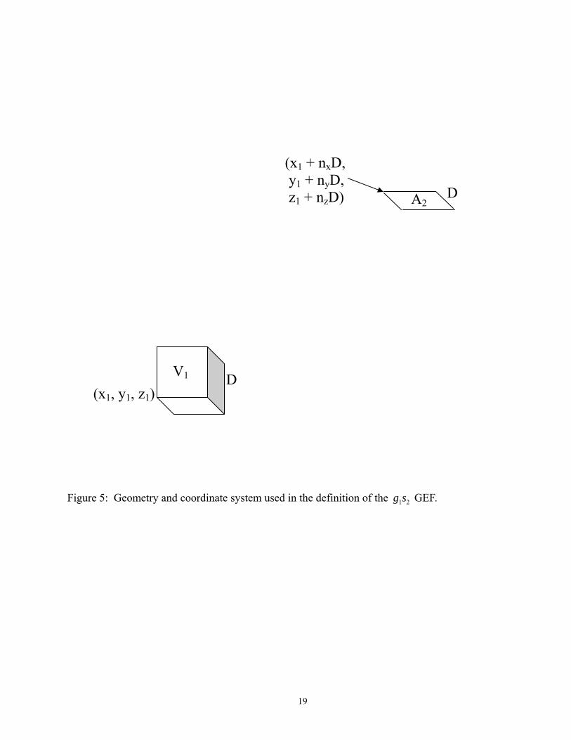
The exchange factor 1 2g s can be similarly expressed in a dimensionless form. Using the

geometry as shown in Figure 5, two partial exchange factors, ( )1 2 zg s and ( )1 2 x

g s , are introduced.

Physically, the partial exchange factor ( )1 2 zg s represents the radiative exchange between 1V and

2A consisting only of those energy rays which pass through the top surface of V1 (z = z1 +D).

The factor ( )1 2 xg s , on the other hand, represents the radiative exchange between 1V and 2A

consisting only of those energy rays which pass through the “x-direction” side surface of V1 (x =

x1 +D). Assuming that the absorption coefficient of the intervening medium is constant (but

different for the two partial exchange factors), the two partial exchange factors can be expressed

in the following dimensionless form

( ) ( )1 2

1 ,2 , , , ,zgsz m z x y z

g sF a D a D n n n

D= (14a)

( ) ( )1 2

1 ,2 , , , ,xgsx m x x y z

g sF a D a D n n n

D= (14b)

Note that in Figure 5, the area 2A is assumed to be parallel to the x-y plane. For general

application, there is no loss of generality since a discretized area is always parallel to one of the

face of the discretized volume in a rectangular coordinate system with equal grid size. The two

average absorption coefficients are taken along the two line of sights directed toward the center

of the receiving plane, from the top area element (z = z1 +D) and x-direction side area element

(x = x1 +D) respectively. Similar to Eq. (13), the exchange factor between between 1V and 2A

can be generated by superposition as

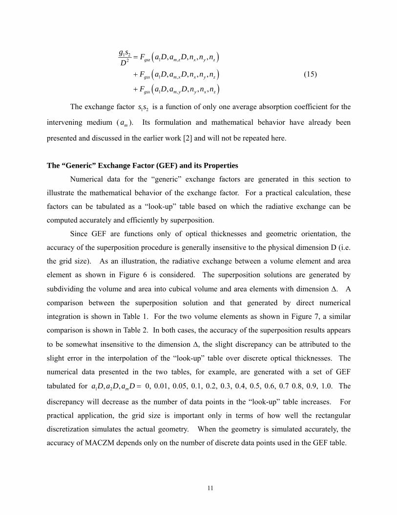
11

( )( )( )

1 21 ,2

1 ,

1 ,

, , , ,

, , , ,

, , , ,

gsz m z x y z

gsx m x x y z

gsx m y y x z

g s F a D a D n n nD

F a D a D n n n

F a D a D n n n

=

+

+

(15)

The exchange factor 1 2s s is a function of only one average absorption coefficient for the

intervening medium ( ma ). Its formulation and mathematical behavior have already been

presented and discussed in the earlier work [2] and will not be repeated here.

The “Generic” Exchange Factor (GEF) and its Properties

Numerical data for the “generic” exchange factors are generated in this section to

illustrate the mathematical behavior of the exchange factor. For a practical calculation, these

factors can be tabulated as a “look-up” table based on which the radiative exchange can be

computed accurately and efficiently by superposition.

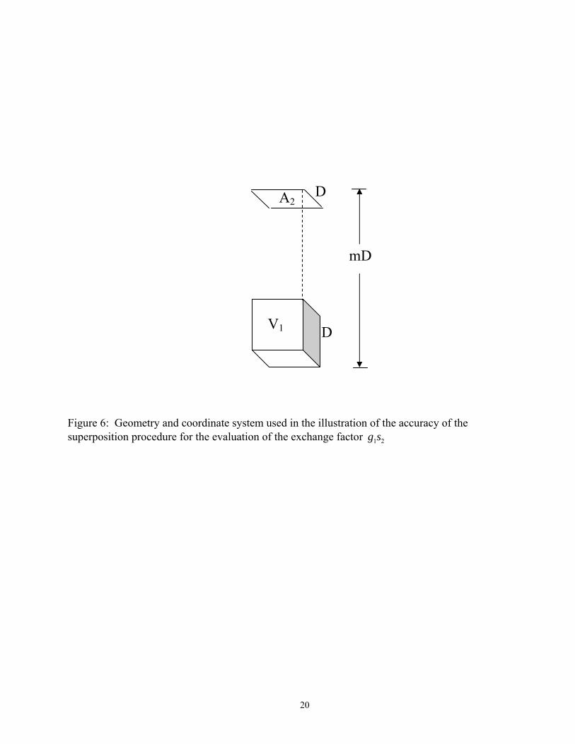
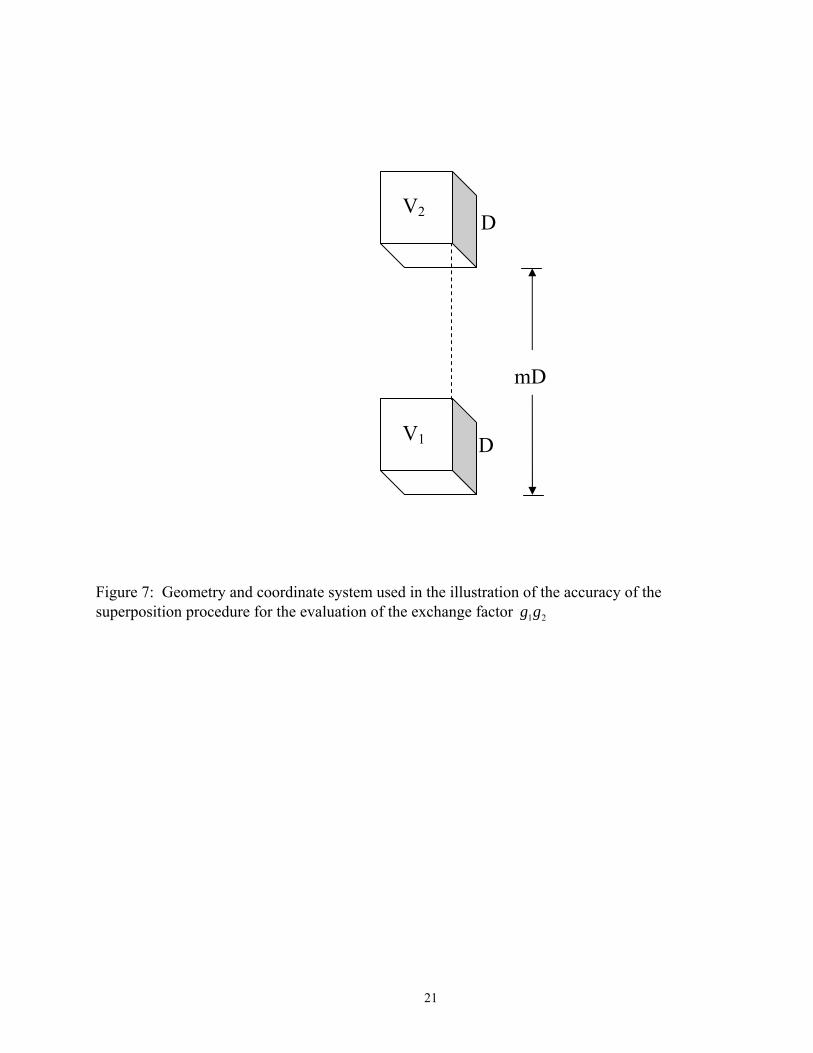
Since GEF are functions only of optical thicknesses and geometric orientation, the

accuracy of the superposition procedure is generally insensitive to the physical dimension D (i.e.

the grid size). As an illustration, the radiative exchange between a volume element and area

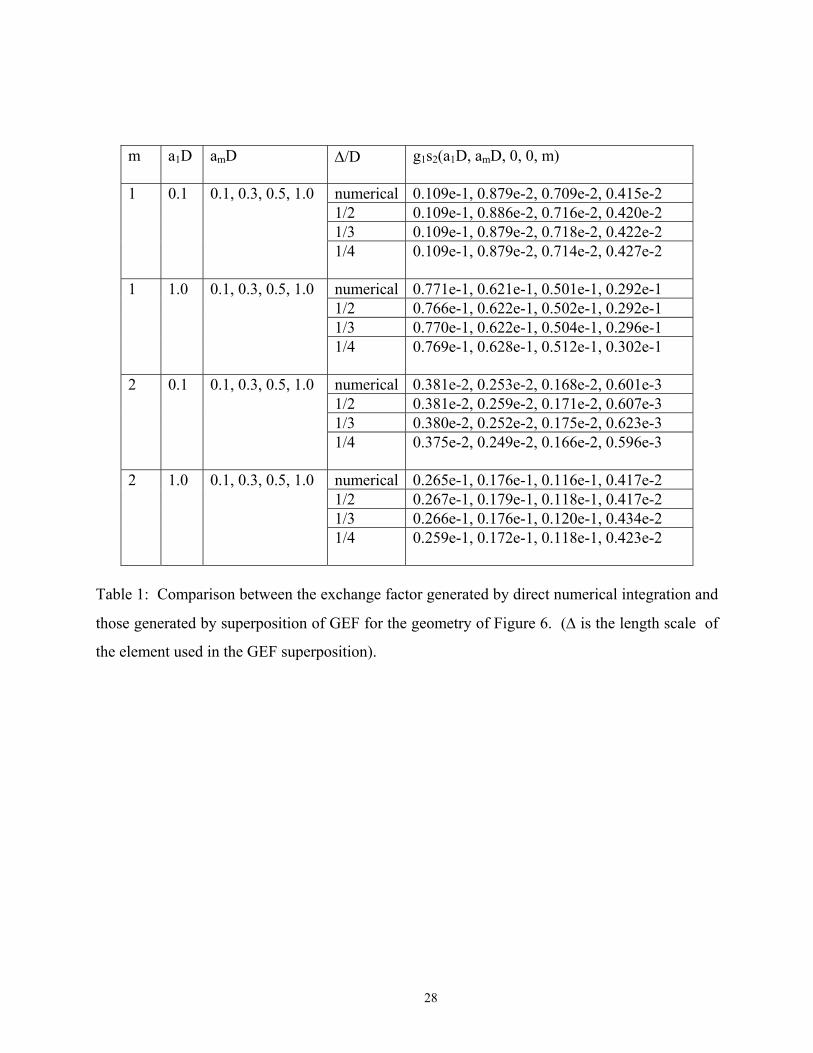
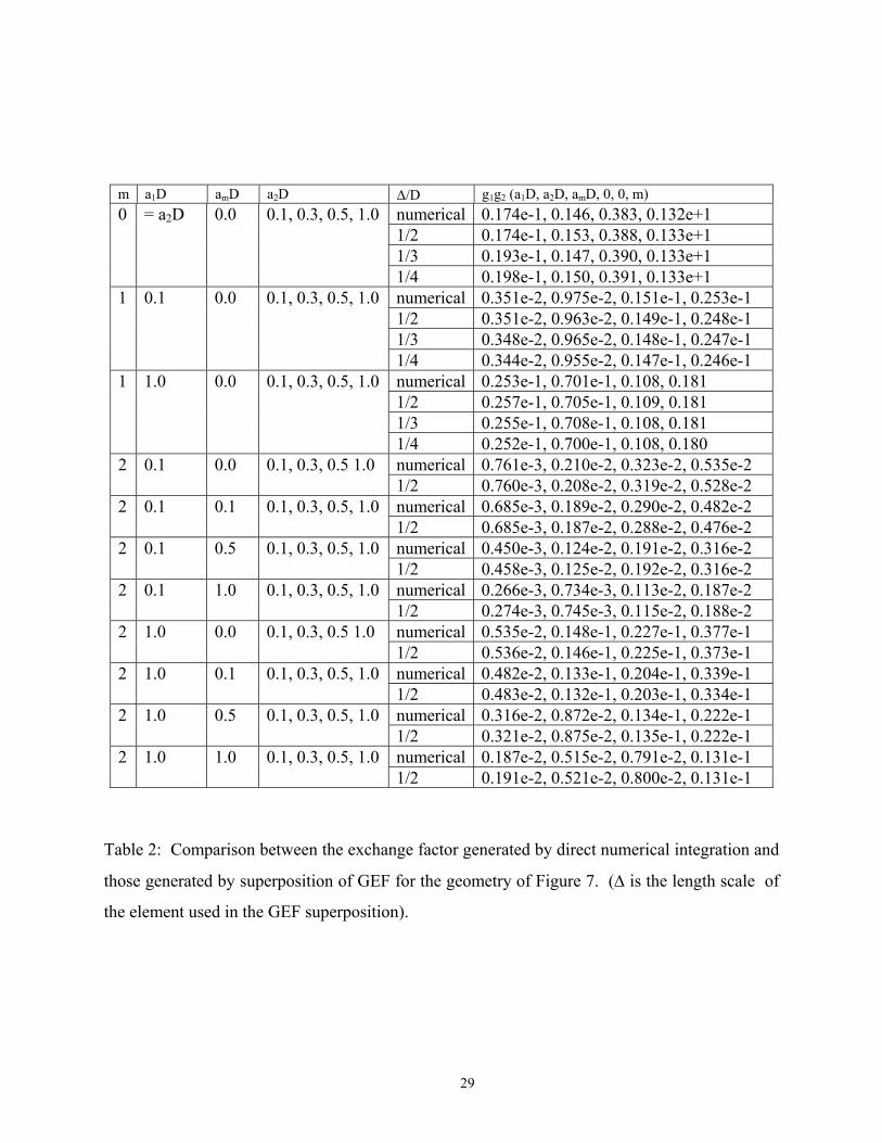
element as shown in Figure 6 is considered. The superposition solutions are generated by

subdividing the volume and area into cubical volume and area elements with dimension ∆. A

comparison between the superposition solution and that generated by direct numerical

integration is shown in Table 1. For the two volume elements as shown in Figure 7, a similar

comparison is shown in Table 2. In both cases, the accuracy of the superposition results appears

to be somewhat insensitive to the dimension ∆, the slight discrepancy can be attributed to the

slight error in the interpolation of the “look-up” table over discrete optical thicknesses. The

numerical data presented in the two tables, for example, are generated with a set of GEF

tabulated for 1 2, , ma D a D a D = 0, 0.01, 0.05, 0.1, 0.2, 0.3, 0.4, 0.5, 0.6, 0.7 0.8, 0.9, 1.0. The

discrepancy will decrease as the number of data points in the “look-up” table increases. For

practical application, the grid size is important only in terms of how well the rectangular

discretization simulates the actual geometry. When the geometry is simulated accurately, the

accuracy of MACZM depends only on the number of discrete data points used in the GEF table.

12

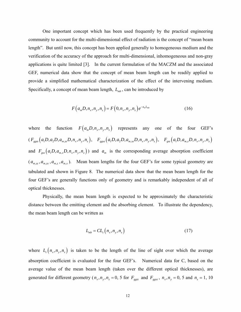
One important concept which has been used frequently by the practical engineering

community to account for the multi-dimensional effect of radiation is the concept of “mean beam

length”. But until now, this concept has been applied generally to homogeneous medium and the

verification of the accuracy of the approach for multi-dimensional, inhomogeneous and non-gray

applications is quite limited [3]. In the current formulation of the MACZM and the associated

GEF, numerical data show that the concept of mean beam length can be readily applied to

provide a simplified mathematical characterization of the effect of the intervening medium.

Specifically, a concept of mean beam length, mbL , can be introduced by

( ) ( ), , , 0, , , m mba Lm x y z x y zF a D n n n F n n n e−= (16)

where the function ( ), , ,m x y zF a D n n n represents any one of the four GEF’s

( ( )1 2 ,, , , , ,ggzz m zz x y zF a D a D a D n n n , ( )1 2 ,, , , , ,ggxz m xz x y zF a D a D a D n n n , ( )1 ,, , , ,gsz m z x y zF a D a D n n n

and ( )1 ,, , , ,gsx m x x y zF a D a D n n n ) and ma is the corresponding average absorption coefficient

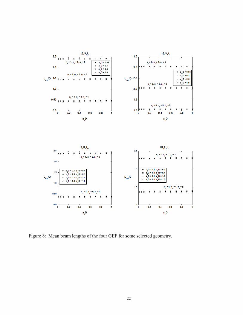
( ,m zza , ,m zxa , ,m za , ,m xa ). Mean beam lengths for the four GEF’s for some typical geometry are

tabulated and shown in Figure 8. The numerical data show that the mean beam length for the

four GEF’s are generally functions only of geometry and is remarkably independent of all of

optical thicknesses.

Physically, the mean beam length is expected to be approximately the characteristic

distance between the emitting element and the absorbing element. To illustrate the dependency,

the mean beam length can be written as

( ), ,mb c x y zL CL n n n= (17)

where ( ), ,c x y zL n n n is taken to be the length of the line of sight over which the average

absorption coefficient is evaluated for the four GEF’s. Numerical data for C, based on the

average value of the mean beam length (taken over the different optical thicknesses), are

generated for different geometry ( , ,x y zn n n = 0, 5 for ggzzF and ggxzF , ,x yn n = 0, 5 and zn = 1, 10

13

for gsxF and gszF ). These data are plotted collectively against a single variable ( zn ) in Figure 9.

It is interesting to note that C is close to unity and is approximately constant except for

configurations in which the emitting and absorbing elements are close to each other. For

combustion gases, this mathematical behavior of C can be utilized to develop band correlation to

characterize the absorption of the intervening gas. This effort is currently under consideration

and will be presented in future publications. APPLICATION MACZM is applied to analyze the effect of radiation on the mixing of hot molten fuel

with water. For simplicity, the radiative absorption of steam is neglected in the calculation. The

detailed analysis and results will be presented in future publications. In the present work, the

predicted radiative heat transfer distribution is presented to illustrate the effectiveness of

MACZM.

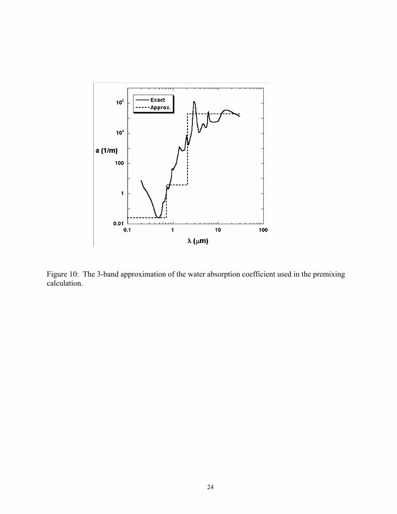
Because of the large variation of the absorption coefficient of water over the wavelength

of interest as shown in Figure 1, a three-band approach is used to capture the difference in

radiative energy distribution in the different wavelength region. The step wise approximation

used for the absorption coefficient of water is shown in Figure 10. The absorption coefficients

of the three bands correspond to the absorption coefficient of three characteristic wavelengths

0.4915 µm, 0.9495 µm and 3.277 µm respectively. The middle wavelength (0.9495 µm) is the

wavelength at which the blackbody emissive power at the molten fuel temperature (3052 K) is a

maximum. The fractions of energy radiated by the molten fuel (at 3052 K) for the three bands

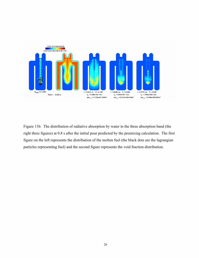
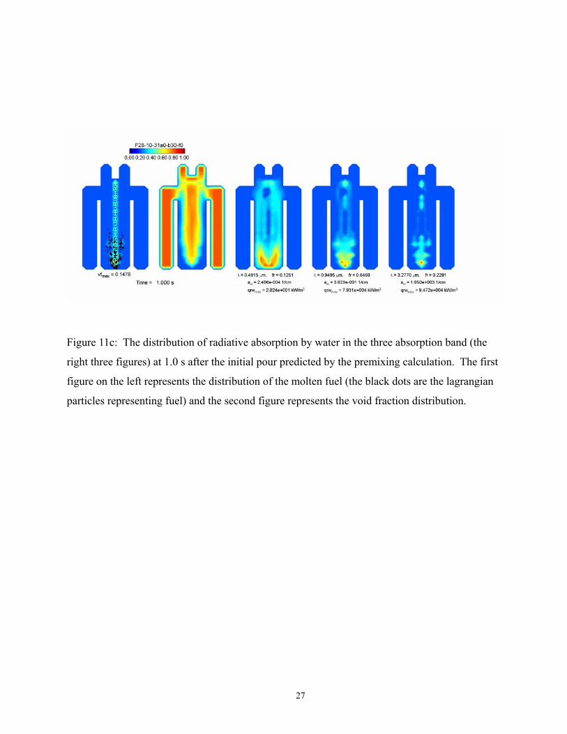
are 0.125, 0.647 and 0.228 respectively. Using a grid size of 10 cm (with the inner vessel

diameter of 70 cm), the rate of energy absorption by water predicted for three different times

during the premixing transient are shown in Figures 11a, 11b and 11c. It can be readily observed

that the distribution of water energy absorption varies significantly among the three bands. In

the first band at which water is optically transparent, the radiation penetrates a significant

distance away from the radiating molten fuel. This accounts for the “red hot” visual appearance

commonly observed in the interaction of high temperature molten fuel and water. The first band,

however, accounts only for 12.5% of the total energy radiated from the fuel. For the remaining

energy, the water absorption coefficient is high and the water absorption is highly localized in

the region surrounding the fuel. The localized absorption appears to dominate the boiling

14

process as the second and third band account for more than 80% of the radiative emission.

MACZM captures both the transient and spatial distribution of the radiative absorption

distribution accurately and efficiently.

Because of the large variation of the water absorption coefficient over wavelength and

the large values of the water absorption coefficient in the long wavelength region, a larger

number of band and smaller grid size are needed to simulate accurately the effect of radiation on

the premixing process. This effort is currently underway and results will be presented in future

publications.

CONCLUSION The formulation of a multiple absorption coefficient zonal method (MACZM) is

presented. Four “generic” exchange factors (GEF) are shown to be accurate and effective in

simulating the radiative exchange. Numerical values these GEF’s are tabulated and their

mathematical behavior is described. The concept of mean beam length is shown to be effective

in separating the effect of the intervening absorption coefficient on the radiative exchange.

MACZM is shown to be effective in capturing the physics of radiative heat transfer in a

multi-dimensional inhomogeneous three phase mixture (molten fuel, liquid and vapor) generated

in the premixing phase of a steam explosion.

REFERENCES 1. Hottel, H. C. and Sarofim, A. F., “Radiative Transfer”, McGraw Hill, New York, 1967.

2. Yuen, W. W. and Takara, E. E. “The Zonal Method, a Practical Solution Method for Radiative

Transfer in Non-Isothermal Inhomogeneous Media”, Annual Review of Heat Transfer, Vol. 8

(1997), pp. 153-215.

3. Siegel, R. and Howell, J. R., “Thermal Radiation Heat Transfer”, 4th Ed., Taylor and Francis,

New York, 2002.

15

Figure 1: The absorption coefficient of water and the blackbody emissive power at 3052 K.

16

Figure 2: The distribution of molten UO2 (left, with the black dot representing the “fuel” as lagrangian particles) and the void fraction distribution of water (right) during a premixing process.

17

Figure 3: Example geometry highlighting the difference in “average absorption coefficient” for different optical path.

D

D

3D

3D S1

S2

V1

V2

18

Figure 4: Geometry and coordinate system used in the definition of the 1 2g g GEF.

D

D(x1 + nxD, y1 + nyD, z1 + nzD)

(x1,y1,z1) V1

V2

19

Figure 5: Geometry and coordinate system used in the definition of the 1 2g s GEF.

D(x1, y1, z1)

V1

D A2

(x1 + nxD, y1 + nyD, z1 + nzD)

20

Figure 6: Geometry and coordinate system used in the illustration of the accuracy of the superposition procedure for the evaluation of the exchange factor 1 2g s

DV1

DA2

mD

21

Figure 7: Geometry and coordinate system used in the illustration of the accuracy of the superposition procedure for the evaluation of the exchange factor 1 2g g

DV1

D

mD

V2

22

Figure 8: Mean beam lengths of the four GEF for some selected geometry.

23

Figure 9: Values of /mb cL L of the four GEF for different values of , ,x y zn n n .

24

Figure 10: The 3-band approximation of the water absorption coefficient used in the premixing calculation.

25

Figure 11a: The distribution of radiative absorption by water in the three absorption band (the

right three figures) at 0.6 s after the initial pour predicted by the premixing calculation. The first

figure on the left represents the distribution of the molten fuel (the black dots are the lagrangian

particles representing fuel) and the second figure represents the void fraction distribution.

26

Figure 11b: The distribution of radiative absorption by water in the three absorption band (the




27

Figure 11c: The distribution of radiative absorption by water in the three absorption band (the




28

m

a1D amD ∆/D g1s2(a1D, amD, 0, 0, m)

numerical 0.109e-1, 0.879e-2, 0.709e-2, 0.415e-2 1/2 0.109e-1, 0.886e-2, 0.716e-2, 0.420e-2 1/3 0.109e-1, 0.879e-2, 0.718e-2, 0.422e-2

1 0.1 0.1, 0.3, 0.5, 1.0

1/4 0.109e-1, 0.879e-2, 0.714e-2, 0.427e-2


1 1.0 0.1, 0.3, 0.5, 1.0

1/4 0.769e-1, 0.628e-1, 0.512e-1, 0.302e-1


2 0.1 0.1, 0.3, 0.5, 1.0

1/4 0.375e-2, 0.249e-2, 0.166e-2, 0.596e-3


2 1.0 0.1, 0.3, 0.5, 1.0

1/4 0.259e-1, 0.172e-1, 0.118e-1, 0.423e-2

Table 1: Comparison between the exchange factor generated by direct numerical integration and

those generated by superposition of GEF for the geometry of Figure 6. (∆ is the length scale of

the element used in the GEF superposition).

29

m a1D amD a2D ∆/D g1g2 (a1D, a2D, amD, 0, 0, m) numerical 0.174e-1, 0.146, 0.383, 0.132e+1 1/2 0.174e-1, 0.153, 0.388, 0.133e+1 1/3 0.193e-1, 0.147, 0.390, 0.133e+1

0 = a2D 0.0 0.1, 0.3, 0.5, 1.0

1/4 0.198e-1, 0.150, 0.391, 0.133e+1 numerical 0.351e-2, 0.975e-2, 0.151e-1, 0.253e-1 1/2 0.351e-2, 0.963e-2, 0.149e-1, 0.248e-1 1/3 0.348e-2, 0.965e-2, 0.148e-1, 0.247e-1

1 0.1 0.0 0.1, 0.3, 0.5, 1.0

1/4 0.344e-2, 0.955e-2, 0.147e-1, 0.246e-1 numerical 0.253e-1, 0.701e-1, 0.108, 0.181 1/2 0.257e-1, 0.705e-1, 0.109, 0.181 1/3 0.255e-1, 0.708e-1, 0.108, 0.181

1 1.0 0.0 0.1, 0.3, 0.5, 1.0

1/4 0.252e-1, 0.700e-1, 0.108, 0.180 numerical 0.761e-3, 0.210e-2, 0.323e-2, 0.535e-2 2 0.1 0.0 0.1, 0.3, 0.5 1.0 1/2 0.760e-3, 0.208e-2, 0.319e-2, 0.528e-2 numerical 0.685e-3, 0.189e-2, 0.290e-2, 0.482e-2 2 0.1 0.1 0.1, 0.3, 0.5, 1.0 1/2 0.685e-3, 0.187e-2, 0.288e-2, 0.476e-2 numerical 0.450e-3, 0.124e-2, 0.191e-2, 0.316e-2 2 0.1 0.5 0.1, 0.3, 0.5, 1.0 1/2 0.458e-3, 0.125e-2, 0.192e-2, 0.316e-2 numerical 0.266e-3, 0.734e-3, 0.113e-2, 0.187e-2 2 0.1 1.0 0.1, 0.3, 0.5, 1.0 1/2 0.274e-3, 0.745e-3, 0.115e-2, 0.188e-2 numerical 0.535e-2, 0.148e-1, 0.227e-1, 0.377e-1 2 1.0 0.0 0.1, 0.3, 0.5 1.0 1/2 0.536e-2, 0.146e-1, 0.225e-1, 0.373e-1 numerical 0.482e-2, 0.133e-1, 0.204e-1, 0.339e-1 2 1.0 0.1 0.1, 0.3, 0.5, 1.0 1/2 0.483e-2, 0.132e-1, 0.203e-1, 0.334e-1 numerical 0.316e-2, 0.872e-2, 0.134e-1, 0.222e-1 2 1.0 0.5 0.1, 0.3, 0.5, 1.0 1/2 0.321e-2, 0.875e-2, 0.135e-1, 0.222e-1 numerical 0.187e-2, 0.515e-2, 0.791e-2, 0.131e-1 2 1.0 1.0 0.1, 0.3, 0.5, 1.0 1/2 0.191e-2, 0.521e-2, 0.800e-2, 0.131e-1

Table 2: Comparison between the exchange factor generated by direct numerical integration and

those generated by superposition of GEF for the geometry of Figure 7. (∆ is the length scale of

the element used in the GEF superposition).

the multiple absorption coefficient zonal method …yuen/current_paper/zonal_nht.pdfwalter w. yuen...

Documents