The Midterm Review

spring 2013

Featuring a very fine set of example problems

Several failed attempts at simplexing

Our Feature Presentation

1. Simplexing to glory – see previous presentation 2. Transporting in an optimal manner 3. Engineering assignments 4. Networking on the shortest path 5. Spanning the tree 6. Maximum flow 7. Linear Formulating

OR students anxious to work the midterm

2. The Transportation Algorithm

Shipping a single commodity from several sources to several destinations in an optimal manner.

(a) The northwest corner

factory Store 1 Store 2 Store 3 Store 4 Store 5 Supply

ABC 9 10 12 8 0 19

DEF 15 14 15

13

0 13

XYZ 15 13 10 12 0

17

Demand 10 11 15 6 7

(a) The northwest corner

factory Store 1 Store 2 Store 3 Store 4 Store 5 Supply

ABC 9

10 10

9 12 8 0 19

DEF 15 14

2 15

11 13

0 13

XYZ 15 13 10

4 12

6 0

7 17

Demand 10 11 15 6 7

(a) The northwest corner

factory Store 1 Store 2 Store 3 Store 4 Store 5 Supply

ABC 9

10 10

9 12

1

8

-5

0

-1

19

DEF 15

+

14

2 15

11 13

-4

0

-5

13

XYZ 15

+

13

+

10

4 12

6 0

7 17

Demand 10 11 15 6 7

(a) The northwest corner

factory Store 1 Store 2 Store 3 Store 4 Store 5 Supply

ABC 9

10 10

9 12 8

+

0 19

DEF 15 14

2 15

11 13 0 13

XYZ 15 13 10

4 12

6 0

7 17

Demand 10 11 15 6 7

(b) Our very first (and last) iteration

factory Store 1 Store 2

Store 3 Store 4 Store 5 Supply

ABC 9

10 10

3 12

+

8

6 0

-1

19

DEF 15

+

14

8 15

5 13

+

0

-5

13

XYZ 15

+

13

+

10

10 12

+

0

7 17

Demand 10 11 15 6 7 49

(c) Show the reduction in cost: 6 units x -$5 = -$30 (d) Is the solution in (b) optimal? No, see cell negative costing

PISONIT Ratings

Engineer Project

A

Project B Project C Project D Project E Project F

Bill 80 72 65 41 39 54

Betty 82 81 56 52 28 60

Bob 77 64 45 62 25 43

Bertha 72 68 71 61 37 64

Bull 68 60 32 38 19 40

• Determine which engineer is to be assigned to each project in order to maximize the sum of the individual scores. • Scores are based upon the job Propensity Index Standard Of the National Institute of Technology (PISONIT). • Makes use of the engineer’s experience, education, and skill sets and how well they match the engineering requirements of the project.

We start…

by subtracting each value in a row or column from the maximum value to convert to a minimization problem and to obtain a zero in each row or column and then add a dummy row:

0 8 15 39 41 26 0 1 26 30 54 22 0 13 32 15 52 34 0 4 1 11 35 8 0 8 36 30 49 28 0 0 0 0 0 0

Engineer Project A Project B Project C Project D Project E Project F

Bill 80 72 65 41 39 54

Betty 82 81 56 52 28 60

Bob 77 64 45 62 25 43

Bertha 72 68 71 61 37 64

Bull 68 60 32 38 19 40

Still starting… Need to create more strategic zero cells:

0 8 15 39 41 26 0 1 26 30 54 22 0 13 32 15 52 34 0 4 1 11 35 8 0 8 36 30 49 28 0 0 0 0 0 0

0 7 15 38 40 25 0 0 25 29 53 21 0 12 31 14 51 33 0 3 0 10 34 7 0 7 35 29 48 27 1 0 0 0 0 0

We continue…

0 7 15 31 33 18 0 0 25 22 46 14 0 12 31 7 44 26 0 3 0 3 27 0 0 7 35 22 41 20 8 7 7 0 0 0

0 7 15 38 40 25 0 0 25 29 53 21 0 12 31 14 51 33 0 3 0 10 34 7 0 7 35 29 48 27 1 0 0 0 0 0

We do it again…

0 7 8 24 26 11 0 0 18 15 39 7 0 12 24 0 37 19 7 10 0 3 27 0 0 7 28 15 34 13 15 14 7 0 0 0

0 7 15 31 33 18 0 0 25 22 46 14 0 12 31 7 44 26 0 3 0 3 27 0 0 7 35 22 41 20 8 7 7 0 0 0

And again…

0 7 1 17 19 4 0 0 11 8 32 0 7 19 24 0 37 19 14 17 0 3 27 0 0 7 21 8 27 6 22 21 7 0 0 0

0 7 8 24 26 11 0 0 18 15 39 7 0 12 24 0 37 19 7 10 0 3 27 0 0 7 28 15 34 13 15 14 7 0 0 0

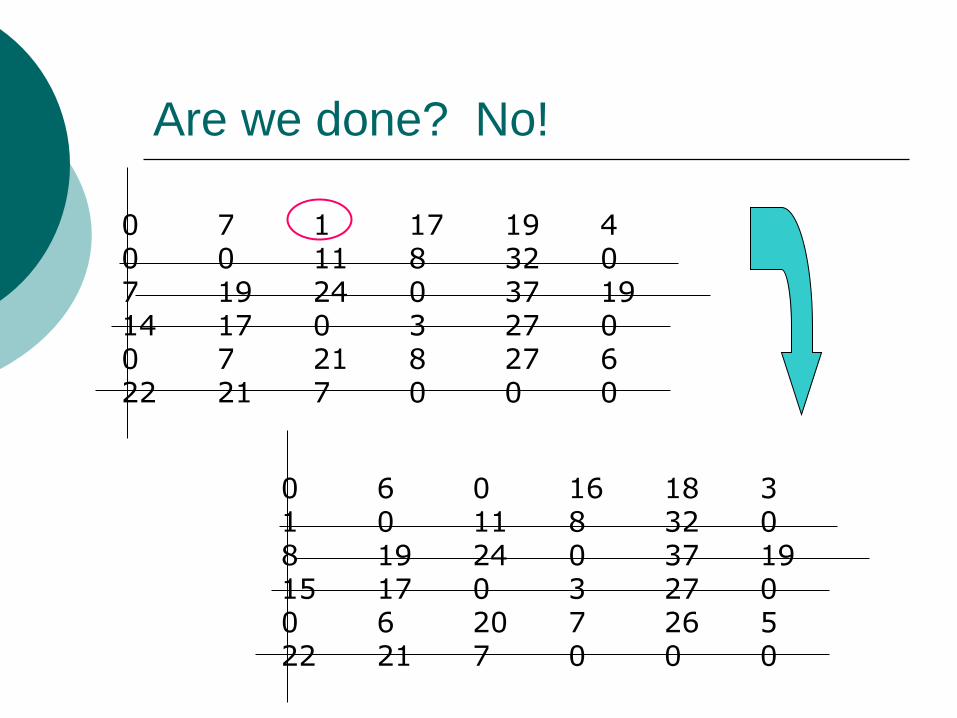
Are we done? No!

0 7 1 17 19 4 0 0 11 8 32 0 7 19 24 0 37 19 14 17 0 3 27 0 0 7 21 8 27 6 22 21 7 0 0 0

0 6 0 16 18 3 1 0 11 8 32 0 8 19 24 0 37 19 15 17 0 3 27 0 0 6 20 7 26 5 22 21 7 0 0 0

Now are we done? Yes!

0 6 0 16 18 3 1 0 11 8 32 0 8 19 24 0 37 19 15 17 0 3 27 0 0 6 20 7 26 5 22 21 7 0 0 0

0 6 0 16 18 3 1 0 11 8 32 0 8 19 24 0 37 19 15 17 0 3 27 0 0 6 20 7 26 5 22 21 7 0 0 0

The Solution

Bill – project C

Betty – Project B

Bob – Project D

Bertha – Project F

Bull – Project A

Dummy – Project E

Engineer Project

A

Project B Project C Project D Project E Project F

Bill 80 72 65 41 39 54

Betty 82 81 56 52 28 60

Bob 77 64 45 62 25 43

Bertha 72 68 71 61 37 64

Bull 68 60 32 38 19 40

Dummy 0 0 0 0 0 0

score = 68 + 81 + 65 + 62 + 64 = 340

4. Networking – the shortest path

Tourist traffic must travel through the county beginning where the interstate system ends (START) and ending at one of Ohio’s best state parks (END). Find the shortest route through the network given below from the Start node to the End node using the algorithm discussed in class. Numbers are distances in miles. The following worktable must be correct to receive full credit.

START

J

I

H

END

G

F

E

D

C

B4 9

7 3

13 11 10 18

14 4 7

23 12 13 14

5 2

12 814

Network for problems 6, 7, and 8.

Networking to a solution

Start B C D E F SD-13 BE-4 CE-4 DG-7 EC-4 FJ-2 SB-14 BF-12 CG-5 DF-11 EB-4 FH-7 SC-23 CF-12 EI-8 D-11 EH-9 FB-12 FC-12 FI-13

G H I J End GJ-3 HF-7 IE-8 JF-2 GC-6 HE-9 IG-10 JG-3 GD-7 HEND-14 IF-13 JEND-18 GI-10 IEND-14

Networking to a solution

14 22 13 18 24 Start B C D E F SD-13 BE-4 CE-4 DG-7 EC-4 FJ-2 SB-14 BF-12 CG-5 DF-11 EB-4 FH-7 SC-23 CF-12 EI-8 D-11 EH-9 FB-12 FC-12 FI-13 20 27 26 23 40 G H I J End GJ-3 HF-7 IE-8 JF-2 GC-6 HE-9 IG-10 JG-3 GD-7 HEND-14 IF-13 JEND-18 GI-10 IEND-14

Shortest Route: Start – B – E – I –End 40 miles

5. Spanning the tree

START

J

I

H

END

G

F

E

D

C

B4 9

7 3

13 11 10 18

14 4 7

23 12 13 14

5 2

12 814

Network for problems 6, 7, and 8.

The tree has been spanned in a

minimal way

START

J

I

H

END

G

F

E

D

C

B4

7 3

13

4 714

5 2

8

Min total distance = 67

6. Maximizing Flow

Determine the maximal flow and the optimum flow in each arc for the following network:

1

4 2

3

5

14

7

5

5 6

7

0

10

8

0

10

0

0

0

9

6

4

0

Max flow working

1

4 2

3

5

14

7

5

5 6

7

0

10

8

0

10

0

0

0

9

6

4

0

Path Flow

1-3-5 10

4

0 10

10

Still working

1

4 2

3

5

14

7

5

5 6

7

0

10

8

0

10

0

0

0

9

6

4

0

Path Flow

1-3-5 10

1-5 4

4

0 10

10

4 0

More still working

1

4 2

3

5

14

7

5

5 6

7

0

10

8

0

10

0 0

0

9

6

4

0

Path Flow

1-3-5 10

1-5 4

1-2-4-5 5

4

0 10

10

4 0

5

0

2

5

11

3

Yes, working

1

4 2

3

5

14

7

5

5 6

7

0

10

8

0

10

0 0

0

9

6

4

0

Path Flow

1-3-5 10

1-5 4

1-2-4-5 5

1-2-5 3

4

0 10

10

4 0

5

0

2

5

11

3 0

8

3

3

Almost done

1

4 2

3

5

14

7

5

5 6

7

0

10

8

0

10

0 0

0

9

6

4

0

Path Flow

1-3-5 10

1-5 4

1-2-4-5 5

1-2-5 3

1-3-2-5 3

4

0 13

10

4 0

5

0

2

5

11

3 0

8

3

6

1

7

8

0

Done! here are the Arc Flows

1

4 2

3

5

14

7

5

5 6

7

0

10

8

0

10

0 0

0

9

6

4

0

Path Flow

1-3-5 10

1-5 4

1-2-4-5 5

1-2-5 3

1-3-2-5 3

25

0 13

10

4 0

5

0 2 11

0

8

6

1

7

8

0

13

4

8

10

6

3

5

5

Linear Formulating

Formulate but do not solve the following linear program:

The CarParts Company manufactures and assembles automobile doors and trunk lids.

The plant produces semi-finished products that are then sanded and painted in the company’s finishing facility. The finishing facility employs a total of 90 workers

in two 8-hour shifts a day, 21 working days a month.

The size of the labor force in the finishing facility fluctuates because of the annual leave taken by the employees.

Formulating with data

May June July

Plant Capacity-doors (# units) 4200 500 6000

Plant Capacity-trunk lids (# units) 3000 2400 2500

Finishing facility leave requests (worker-months*) 30 40 50

Product Unit cost ($) for May

and June

(including labor)

Unit cost ($) for July

(including labor)**

Unit Selling

Price($)

Doors 230 255 450

Trunk lids 180 210 250

Product sales

orders

May June July End-of-April

inventory

Finishing labor

time (minutes)

Doors 3400 3200 3000 70 90

Trunk lids 1500 1400 1200 20 60

The rest of the story… A unit may be produced in one month and held over for

sale in a later month. The storage cost is $5 per month for each door and $4

per month for each trunk lid held over from one month to the next.

Work-in-process floor space within the plant is restricted to 70,000 square feet (i.e. no more than 70,000 sq. ft. of doors and trunk lids can be produced in a given month). Each door requires 11 square feet and each trunk lid

requires 8 square feet.

Warehouse floor space for inventory carried over from one month to the next is limited to 35,000 square feet.

There should be no more than 100 doors and 50 trunk lids available in inventory at the end of July.

No backorders are permitted The Company desires to maximize its profit over the

three-month period. How many doors and trunk lids should be produced each month?

Ahhh, the formulation

(a) Define all decision variables:

X1j = number of doors produced in month j (j=1,2,3)

X2j = number of trunk lids produced in month j (j=1,2,3)

I1j = number of doors in inventory at the end of of month j (j=1,2,3)

I2j = number of trunk lids in inventory at the end of of month j (j=1,2,3)

(b) Formulate the objective function: MAX z = 220X11+220X12+195X13+70X21+70X22

+40X23-5I11-5I12-5I13-4I21-4I22-4I23

Keep on formulating – the constraints

! INVENTORY BALANCE CONSTRAINTS

!I10=70 !I20=20 -I11+X11=3400 - 70 -I12+I11+X12=3200 -I13+I12+X13=3000 I13<100 -I21+X21=1500 - 20 -I22+I21+X22=1400 -I23+I22+X23=1200 I23<50 !LABOR HOUR CONSTRAINTS 1.5X11+X21<10080 (8 x 21 x 60) 1.5X12+X22<8400 (8 x 21 x 50) 1.5X13+X23<6720(8 x 21 x 40)

!STORAGE SPACE CONSTRAINTS 11X11+8X21<70000 11X12+8X22<70000 11X13+8X23<70000 11I11+8I21<35000 11I12+8I22<35000 11I13+8I23<35000 !PLANT CAPACITY CONSTRAINTS X11<4200 X12<500 X13<6000 X21<3000 X22<2400 X23<2500

Another Formulation

The Make-it-Rite Company produces 3 products in 2 factories from iron ore mined in the hills of Pennsylvania.

Given the following data, determine how many tons of each product should be produced monthly in each factory to maximize total profit (selling price minus production and raw material (iron ore) costs.

Iron ore costs $100 per ton and a maximum of 6,000 tons a month is available for distribution to the two factories.

Because of shipping limitations, tons of product A cannot be more than half the total tons of products B and C combined.

The Data

Product Selling price

($) per ton

Maximum

monthly sales

tons of iron ore per ton of

finished product produced

A 350 200 tons 2.5

B 405 150 tons 3.1

C 240 180 tons 1.6

Number Factory Maximum

monthly

production

Production

budget ($)

1 Allentown 200 tons 15,000

2 Pittsburgh 300 tons 20,000

Factory A B C

1 Allentown 65 70 55

2 Pittsburgh 60 75 60

Unit production costs ($/ton)

The Objective Function

Define xi,j = the number of tons of product i produced monthly in factory j where i = A, B, C and j = 1,2 Max z = (350-65-250) xa1 + (405-70-310)xb1 + (240-55-160)xc1 + (350-60-250) xa2 + (405-75-310)xb2 + (240-60-160)xc2 = 35xa1 + 25xb1 + 25xc1 + 40xa2 + 20xb2 + 20xc2

Product Selling price

($) per ton

tons of iron ore per ton of

finished product produced

A 350 2.5

B 405 3.1

C 240 1.6

Iron ore costs $100 per ton

Factory A B C

1 Allentown 65 70 55

2 Pittsburgh 60 75 60

Unit production costs ($/ton)

The Constraints

Max production

xa1 + xb1 + xc1 200

xa2 + xb2 + xc2 300

Max sales

xa1 + xa2 200

xb1 + xb2 150

xc1 + xc2 180

Production budget

65xa1 +70 xb1 +55 xc1 15,000

60xa2 + 75xb2 + 60xc2 20,000

Available iron ore

2.5xa1 + 3.1xb1 + 1.6xc1 + 2.5xa2 + 3.1xb2 + 1.6xc2 6,000

Limit on product A

xa1 + xa2 0.5(xb1 + xb2 + xc1 + xc2)

Prod

uct

Maximum

monthly

sales

tons of iron ore per

ton of finished

product produced

A 200 tons 2.5

B 150 tons 3.1

C 180 tons 1.6

Numbe

r

Factory Maximum

production

budget ($)

1 Allentown 200 tons 15,000

2 Pittsburgh 300 tons 20,000

This has been a Midterm

Review

Brought to you by your friendly engineering management department

Preparing for the midterm