the influence of visibility, cloud ceiling, financial ... · meaning that imc is ... yes yes yes...

A1

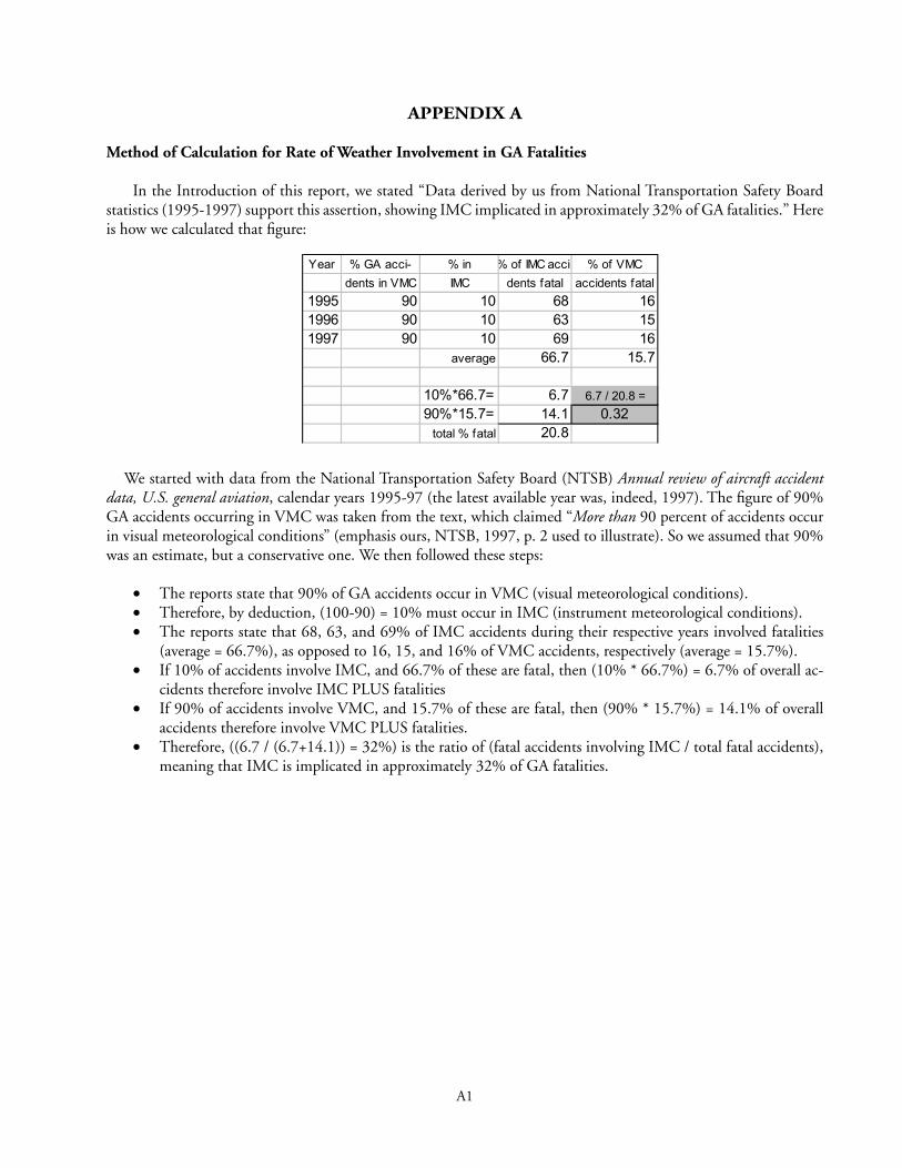
APPENDIX A

Method of Calculation for Rate of Weather Involvement in GA Fatalities

In the Introduction of this report, we stated “Data derived by us from National Transportation Safety Board statistics (1995-1997) support this assertion, showing IMC implicated in approximately 32% of GA fatalities.” Here is how we calculated that figure:

We started with data from the National Transportation Safety Board (NTSB) Annual review of aircraft accident data, U.S. general aviation, calendar years 1995-97 (the latest available year was, indeed, 1997). The figure of 90% GA accidents occurring in VMC was taken from the text, which claimed “More than 90 percent of accidents occur in visual meteorological conditions” (emphasis ours, NTSB, 1997, p. 2 used to illustrate). So we assumed that 90% was an estimate, but a conservative one. We then followed these steps:

• The reports state that 90% of GA accidents occur in VMC (visual meteorological conditions).• Therefore, by deduction, (100-90) = 10% must occur in IMC (instrument meteorological conditions).• The reports state that 68, 63, and 69% of IMC accidents during their respective years involved fatalities

(average = 66.7%), as opposed to 16, 15, and 16% of VMC accidents, respectively (average = 15.7%).• If 10% of accidents involve IMC, and 66.7% of these are fatal, then (10% * 66.7%) = 6.7% of overall ac-

cidents therefore involve IMC PLUS fatalities• If 90% of accidents involve VMC, and 15.7% of these are fatal, then (90% * 15.7%) = 14.1% of overall

accidents therefore involve VMC PLUS fatalities.• Therefore, ((6.7 / (6.7+14.1)) = 32%) is the ratio of (fatal accidents involving IMC / total fatal accidents),

meaning that IMC is implicated in approximately 32% of GA fatalities.

Year % GA acci- % in % of IMC acci- % of VMCdents in VMC IMC dents fatal accidents fatal

1995 90 10 68 161996 90 10 63 151997 90 10 69 16

average 66.7 15.7

10%*66.7= 6.7 6.7 / 20.8 =90%*15.7= 14.1 0.32

total % fatal 20.8

B1

APPENDIX B

Participant Debrief Form

S # ________

q What is your own normal personal minimum for VFR visibility? ________q Your normal personal minimum for VFR cloud ceiling ________q Are these minimums rock-solid, or do you adjust them a little, depending on the circumstances?________q Have you ever flown this particular route before (or a similar situation)? ________q Did the distance you had to fly through bad weather affect your willingness to take off ? ________ (for example,

if the distance had been greater, would you have been even less inclined to take off than you were?)q If you were in the “high-incentive” condition, did this affect your willingness to take off? ________q Do you think having passengers would affect your willingness to take off? (increase it ____, no change____,

decrease it ____)q If you had a lot more flight hours, would that have change your willingness to take off? (increase it ____, no

change____, decrease it ____)q If your flight mission had been critical (for example, delivering a human heart for surgery), would that change

your willingness to take off? (increase it ____, no change____, decrease it ____)q Have you ever flown a Piper Malibu before?_____ Did this affect your willingness to take off?q It made me more willing because I was anxious to try it out ___, q It didn’t matter one way or the other ___, q It made me less willing because I was afraid I’d make more mistakes ___q Did the fact that this was a simulation (and not reality) affect your willingness to take off? q It increased willingness because

q (a) I wanted to fly the sim___ and/or q (b) I knew I couldn’t really get injured in it___,

q No, it had no effect because q (a) it didn’t matter to me one way or the other___q (b) there were positives and negatives but they cancelled each other out___

q It decreased willingness becauseq (a) I was unfamiliar with this particular simulator___q (b) I didn’t want to make any mistakes in front of the experimenter___

q How economically significant was the money to you? 1__not at all 2__a little 3__fairly significant 4__significant 5__very significantq If you were to crash in the simulator, how embarrassed would you be? 1__not at all 2__a little 3__fairly 4__significantly 5__extremelyq Have you ever had a bad flight experience related to weather?___If so, please describe briefly below.

C1

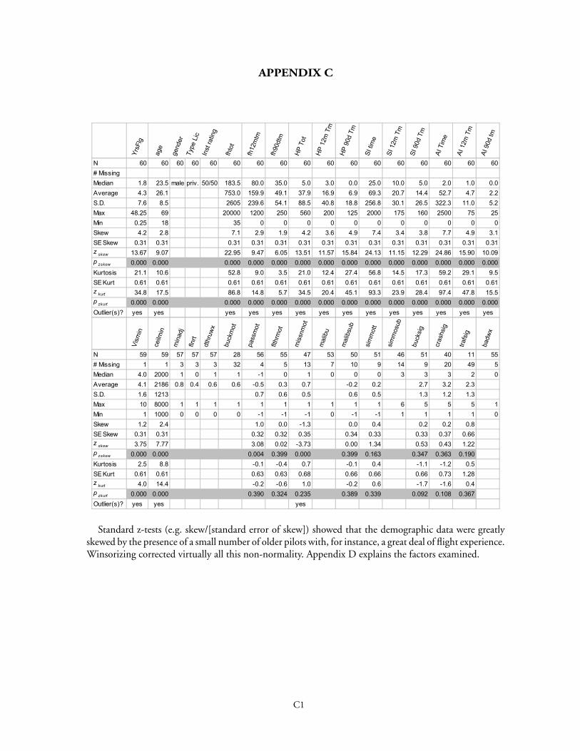
APPENDIX C

Standard z-tests (e.g. skew/[standard error of skew]) showed that the demographic data were greatly skewed by the presence of a small number of older pilots with, for instance, a great deal of flight experience. Winsorizing corrected virtually all this non-normality. Appendix D explains the factors examined.

YrsF

lg

age

gend

erTy

peLi

cIn

stra

ting

fhto

t

fh12

mtm

fh90

dtm

HP

Tot

HP

12m

Tm

HP

90d

Tm

SItim

e

SI12

mTm

SI90

dTm

AITi

me

AI12

mTm

AI90

dtm

N 60 60 60 60 60 60 60 60 60 60 60 60 60 60 60 60 60# MissingMedian 1.8 23.5 male priv. 50/50 183.5 80.0 35.0 5.0 3.0 0.0 25.0 10.0 5.0 2.0 1.0 0.0Average 4.3 26.1 753.0 159.9 49.1 37.9 16.9 6.9 69.3 20.7 14.4 52.7 4.7 2.2S.D. 7.6 8.5 2605 239.6 54.1 88.5 40.8 18.8 256.8 30.1 26.5 322.3 11.0 5.2Max 48.25 69 20000 1200 250 560 200 125 2000 175 160 2500 75 25Min 0.25 18 35 0 0 0 0 0 0 0 0 0 0 0Skew 4.2 2.8 7.1 2.9 1.9 4.2 3.6 4.9 7.4 3.4 3.8 7.7 4.9 3.1SE Skew 0.31 0.31 0.31 0.31 0.31 0.31 0.31 0.31 0.31 0.31 0.31 0.31 0.31 0.31z skew 13.67 9.07 22.95 9.47 6.05 13.51 11.57 15.84 24.13 11.15 12.29 24.86 15.90 10.09p zskew 0.000 0.000 0.000 0.000 0.000 0.000 0.000 0.000 0.000 0.000 0.000 0.000 0.000 0.000Kurtosis 21.1 10.6 52.8 9.0 3.5 21.0 12.4 27.4 56.8 14.5 17.3 59.2 29.1 9.5SE Kurt 0.61 0.61 0.61 0.61 0.61 0.61 0.61 0.61 0.61 0.61 0.61 0.61 0.61 0.61z kurt 34.8 17.5 86.8 14.8 5.7 34.5 20.4 45.1 93.3 23.9 28.4 97.4 47.8 15.5p zkurt 0.000 0.000 0.000 0.000 0.000 0.000 0.000 0.000 0.000 0.000 0.000 0.000 0.000 0.000Outlier(s)? yes yes yes yes yes yes yes yes yes yes yes yes yes yes

Vism

in

ceilm

in

min

adj

flnrt

dthr

uwx

buck

mot

pass

mot

flthr

mot

mis

snm

ot

mal

ibu

mal

ibsu

b

sim

mot

t

sim

mos

ub

buck

sig

cras

hsig

trafs

ig

badw

x

N 59 59 57 57 57 28 56 55 47 53 50 51 46 51 40 11 55# Missing 1 1 3 3 3 32 4 5 13 7 10 9 14 9 20 49 5Median 4.0 2000 1 0 1 1 -1 0 1 0 0 0 3 3 3 2 0Average 4.1 2186 0.8 0.4 0.6 0.6 -0.5 0.3 0.7 -0.2 0.2 2.7 3.2 2.3S.D. 1.6 1213 0.7 0.6 0.5 0.6 0.5 1.3 1.2 1.3Max 10 8000 1 1 1 1 1 1 1 1 1 1 6 5 5 5 1Min 1 1000 0 0 0 0 -1 -1 -1 0 -1 -1 1 1 1 1 0Skew 1.2 2.4 1.0 0.0 -1.3 0.0 0.4 0.2 0.2 0.8SE Skew 0.31 0.31 0.32 0.32 0.35 0.34 0.33 0.33 0.37 0.66z skew 3.75 7.77 3.08 0.02 -3.73 0.00 1.34 0.53 0.43 1.22p zskew 0.000 0.000 0.004 0.399 0.000 0.399 0.163 0.347 0.363 0.190Kurtosis 2.5 8.8 -0.1 -0.4 0.7 -0.1 0.4 -1.1 -1.2 0.5SE Kurt 0.61 0.61 0.63 0.63 0.68 0.66 0.66 0.66 0.73 1.28z kurt 4.0 14.4 -0.2 -0.6 1.0 -0.2 0.6 -1.7 -1.6 0.4p zkurt 0.000 0.000 0.390 0.324 0.235 0.389 0.339 0.092 0.108 0.367Outlier(s)? yes yes yes

D1

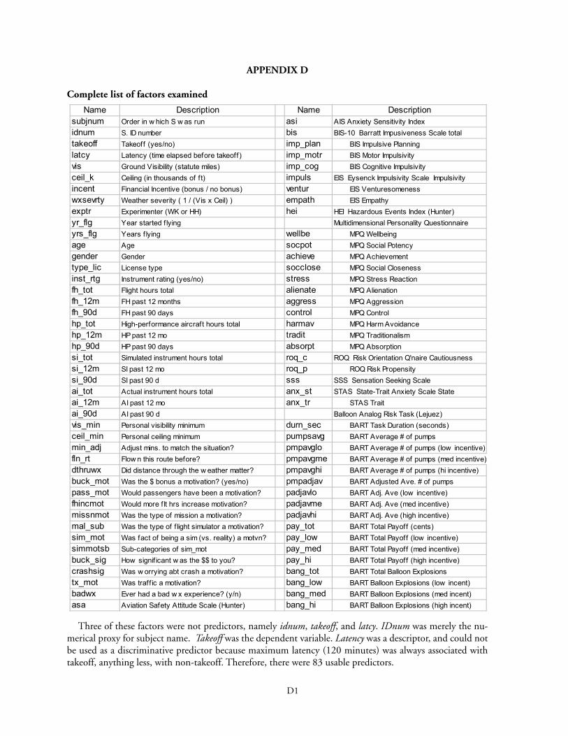
APPENDIX D

Complete list of factors examined

Three of these factors were not predictors, namely idnum, takeoff, and latcy. IDnum was merely the nu-merical proxy for subject name. Takeoff was the dependent variable. Latency was a descriptor, and could not be used as a discriminative predictor because maximum latency (120 minutes) was always associated with takeoff, anything less, with non-takeoff. Therefore, there were 83 usable predictors.

Name Description Name Descriptionsubjnum Order in w hich S w as run asi AIS Anxiety Sensitivity Indexidnum S. ID number bis BIS-10 Barratt Impusiveness Scale totaltakeoff Takeoff (yes/no) imp_plan BIS Impulsive Planninglatcy Latency (time elapsed before takeoff) imp_motr BIS Motor Impulsivityvis Ground Visibility (statute miles) imp_cog BIS Cognitive Impulsivityceil_k Ceiling (in thousands of ft) impuls EIS Eysenck Impulsivity Scale Impulsivityincent Financial Incentive (bonus / no bonus) ventur EIS Venturesomenesswxsevrty Weather severity ( 1 / (Vis x Ceil) ) empath EIS Empathyexptr Experimenter (WK or HH) hei HEI Hazardous Events Index (Hunter)yr_flg Year started f lying Multidimensional Personality Questionnaireyrs_flg Years f lying wellbe MPQ Wellbeingage Age socpot MPQ Social Potencygender Gender achieve MPQ Achievementtype_lic License type socclose MPQ Social Closenessinst_rtg Instrument rating (yes/no) stress MPQ Stress Reactionfh_tot Flight hours total alienate MPQ Alienationfh_12m FH past 12 months aggress MPQ Aggressionfh_90d FH past 90 days control MPQ Controlhp_tot High-performance aircraft hours total harmav MPQ Harm Avoidancehp_12m HP past 12 mo tradit MPQ Traditionalismhp_90d HP past 90 days absorpt MPQ Absorptionsi_tot Simulated instrument hours total roq_c ROQ Risk Orientation Q'naire Cautiousnesssi_12m SI past 12 mo roq_p ROQ Risk Propensitysi_90d SI past 90 d sss SSS Sensation Seeking Scaleai_tot Actual instrument hours total anx_st STAS State-Trait Anxiety Scale Stateai_12m AI past 12 mo anx_tr STAS Trait ai_90d AI past 90 d Balloon Analog Risk Task (Lejuez)vis_min Personal visibility minimum durn_sec BART Task Duration (seconds)ceil_min Personal ceiling minimum pumpsavg BART Average # of pumpsmin_adj Adjust mins. to match the situation? pmpavglo BART Average # of pumps (low incentive)fln_rt Flow n this route before? pmpavgme BART Average # of pumps (med incentive)dthruwx Did distance through the w eather matter? pmpavghi BART Average # of pumps (hi incentive)buck_mot Was the $ bonus a motivation? (yes/no) pmpadjav BART Adjusted Ave. # of pumpspass_mot Would passengers have been a motivation? padjavlo BART Adj. Ave (low incentive)fhincmot Would more flt hrs increase motivation? padjavme BART Adj. Ave (med incentive)missnmot Was the type of mission a motivation? padjavhi BART Adj. Ave (high incentive)mal_sub Was the type of f light simulator a motivation? pay_tot BART Total Payoff (cents)sim_mot Was fact of being a sim (vs. reality) a motvn? pay_low BART Total Payoff (low incentive)simmotsb Sub-categories of sim_mot pay_med BART Total Payoff (med incentive)buck_sig How signif icant w as the $$ to you? pay_hi BART Total Payoff (high incentive)crashsig Was w orrying abt crash a motivation? bang_tot BART Total Balloon Explosionstx_mot Was traff ic a motivation? bang_low BART Balloon Explosions (low incent)badwx Ever had a bad w x experience? (y/n) bang_med BART Balloon Explosions (med incent)asa Aviation Safety Attitude Scale (Hunter) bang_hi BART Balloon Explosions (high incent)

E1

APPENDIX E

Statistical Issues in Logistic Regression Outliers. Outliers are defined for our purposes here as any score greater than 3 standard deviations above or below the mean. Outliers can sometimes exert an almost unbelievable effect on the statistical outcome of an analysis. Take, for example, a distribution of ones and zeros representing Financial Incentive, one of our predictors of Takeoff. For the full data set, N=60, our actual raw distribution yields the following result during SPSS logistic regression:

This result says that the probability of Incentive being a significant predictor of Takeoff is .070.Now let us change one single value in the data distribution from a “0” to a “10” to represent, say, a typographical

error during data coding. Changing just this one value in 60 results in the following:

Suddenly we have gone from p = .070 to p =.894 in one step—by turning a single data point into a gross outlier. Obviously, this says a lot about the need for accurate data coding. It also says quite a bit about how outliers can affect an otherwise normal data distribution. Now logistic regression does not have an underlying logical assumption of normality (Tabachnick & Fidell, 2000). You could, for instance, use data with any relatively symmetrical distribu-tion. But it does have problems with outliers, as this clearly demonstrates.

The data in this study showed outliers in the demographics, where a small number of older pilots significantly skewed the distributions for predictors such as age, flight hours, and years flying. Without some kind of correction, therefore, the effect of outliers would have led us to seriously misinterpret the statistical analysis.

Applying a data transformation (such as a square root or logarithmic function) is a common way to deal with outliers. A somewhat less well-known, but equally respected treatment is winsorization (Winer, 1971, pp 51-54). 1971). In winsorization, the two most-extreme values in the distribution (the one highest and the one lowest) are replaced by a copy of the next most-extreme values. For example, in the distribution

0 1 1 1 2 2 2 2 3 3 3 3 3 3 4 4 4 4 5 5 5 99 (mean 7.23, SD 20.54)

we would replace the “0” with a “1” and the “99” with a “5.”

1 1 1 1 2 2 2 2 3 3 3 3 3 3 4 4 4 4 5 5 5 5 (mean 3.00, SD 1.38)

Now this new distribution is still not normal because it is too flat. But it no longer has the gross outlier it once had. That extreme value of “99” is still represented by a relatively high value, which preserves the ordinality (rank order) of the scores. But notice that there was no actual change to most of the numbers. Only two values were changed, and one of those was a very modest change from a “0” to a “1.” Whereas, if we had applied a mathematical function such as a square root to shrink the “99” closer to the mean, almost all of the values would have been affected. Here winsorization exerts its biggest effect on the greatest offender, which is exactly how data conditioning should work. This illustrates how this technique can sometimes preserve the spirit and actuality of a distribution much better than can some of the more routinely used methods. For this reason, it was the method of choice for our data.

Variables in the Equation

.981 .541 3.287 1 .070 2.667-.847 .398 4.523 1 .033 .429

INCENTConstant

Step1

a

B S.E. Wald df Sig. Exp(B)

Variable(s) entered on step 1: INCENT.a.


-.027 .204 .018 1 .894 .973-.319 .294 1.171 1 .279 .727

INCENTConstant

Step1

a


Variable(s) entered on step 1: INCENT.a.

E2 F1

If a distribution has more than one outlier, say

0 0 1 1 2 2 2 2 3 3 3 3 3 3 4 4 4 4 5 5 47 99 (mean 9.09, SD 22.23)

we simply apply the winsorization procedure twice, to yield

1 1 1 1 2 2 2 2 3 3 3 3 3 3 4 4 4 4 5 5 47 47 (mean 6.82, SD 13.06)

at stage one and

2 2 2 2 2 2 2 2 3 3 3 3 3 3 4 4 4 4 5 5 5 5 (mean 3.18, SD 1.14)

at stage two. In this example, the two-stage winsorization affects 6 values, rather than just 2. For this reason we have to be careful in repeating this process too often, since it can lead to the antithetical problem of range restriction.

In this, study winsorization was limited to no more than 2 stages. For example, in the full data set (N=60) 16 demographic variables were seen to have outliers > 3 SD, and therefore received either a 1- or 2-stage winsorization, depending on what was needed to eliminate these outliers. After treatment, all 16 variables emerged corrected to tolerance.

A final point worth mentioning is that winsorization has a net result of making our statistical analysis more conservative. This happens precisely because the distributions’ ranges and variances contract during conditioning, and any time variance contracts, p-values generally contract as well. This is not true with purely ordinal statistics, because these calculate their value based on nothing more than rank order. But both chi-square and logistic regres-sion do not fall into that category. While logistic regression is often touted as being distribution-free, in fact, we have graphically illustrated that things are a bit more complex. Outliers skew its innermost calculation of likelihood ratios (SPSS, 2004). However, the data conditioning process employed here allowed us to successfully treat data and to present p-values representing useful-yet-conservative estimates of statistical reliability.

Correction for Familywise Error. Another important issue is the one of correcting p-values to account for the number of predictors examined. Most statisticians recommend some sort of correction for experimentwise Type I error (unwarranted rejection of the null hypothesis). Otherwise, if we do many tests, odds are that some will be “significant” simply by chance.

However, we consciously chose to deviate from that standard procedure because, in an exploratory study such as this, such rigor, while admirable in one sense, would most certainly have the net result of too much Type II error, that is, failure to detect a true effect where there was one. And, while the danger of inflated experimentwise Type I error was fully appreciated, we also felt it made more sense to report low p-values where found, because these really do represent the best guess we have regarding effect.

The ideal way to resolve the problem, of course, is to run Monte Carlo simulations to get estimates for mean predictivities and R2s, given specific parameters of specific models. This was done in Part II of this report. Another accepted approach is to replicate studies or parts of studies, using different participants. That will be done in follow-up studies, whenever possible.

E2 F1

APPENDIX F

Brief Description of Logistic Regression Logistic regression is a statistical technique specially constructed for use with discrete dependent variables, for

example, Takeoff versus No Takeoff. It is a very useful technique, but it is also extremely easy to miscode, misunder-stand, and misinterpret. The best way to understand it is through a combination of mathematics and example.

Regression is the search for factors that predict other factors. In this experiment, we wanted to predict the likelihood that an average pilot would take off into known marginal weather, given the added influence of financial incentive. Three of our predictive factors (Visibility, Cloud Ceiling, and Financial Incentive) were under experimental control; the rest reflected either demographic or personality characteristics of each individual pilot.

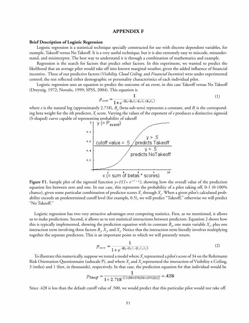
Logistic regression uses an equation to predict the outcome of an event, in this case Takeoff versus No Takeoff (Dreyszig, 1972; Norušis, 1999; SPSS, 2004). This equation is

(1)

where e is the natural log (approximately 2.718), B0 (beta-sub-zero) represents a constant, and B

i is the correspond-

ing beta weight for the ith predictor, Xi score. Varying the values of the exponent of e produces a distinctive sigmoid

(S-shaped) curve capable of representing probability of takeoff

Figure F1. Sample plot of the sigmoid function y=1/(1+ e-(-5 + x)), showing how the overall value of the prediction equation lies between zero and one. In our case, this represents the probability of a pilot taking off, 0-1 (0-100% chance), given some particular combination of predictor scores X

1 through X

n. When a given pilot’s calculated prob-

ability exceeds an predetermined cutoff level (for example, 0.5), we will predict “Takeoff,” otherwise we will predict “No Takeoff.”

Logistic regression has two very attractive advantages over competing statistics. First, as we mentioned, it allows us to make predictions. Second, it allows us to test statistical interactions between predictors. Equation 2 shows how this is typically implemented, showing the prediction equation with its constant B

0, one main variable X

1, plus one

interaction term involving three factors B2, X

2, and X

3. Notice that the interaction term literally involves multiplying

together the separate predictors. This is an important point to which we will presently return.

(2)

To illustrate this numerically, suppose we tested a model where X1 represented a pilot’s score of 34 on the Rohrmann

Risk Orientation Questionnaire (subscale P), and where X2 and X

3 represented the interaction of Visibility x Ceiling,

3 (miles) and 1 (feet, in thousands), respectively. In that case, the prediction equation for that individual would be

Since .428 is less than the default cutoff value of .500, we would predict that this particular pilot would not take off.

F2 F3

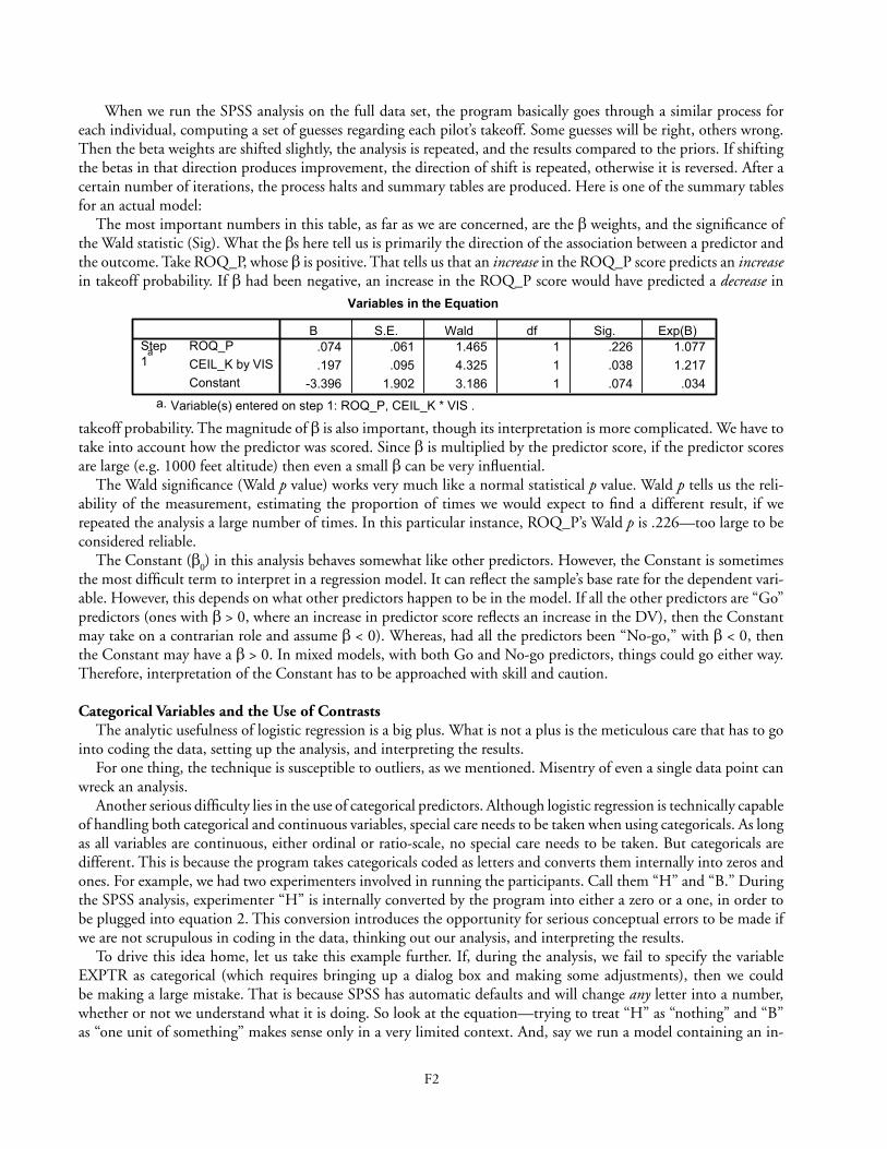
When we run the SPSS analysis on the full data set, the program basically goes through a similar process for each individual, computing a set of guesses regarding each pilot’s takeoff. Some guesses will be right, others wrong. Then the beta weights are shifted slightly, the analysis is repeated, and the results compared to the priors. If shifting the betas in that direction produces improvement, the direction of shift is repeated, otherwise it is reversed. After a certain number of iterations, the process halts and summary tables are produced. Here is one of the summary tables for an actual model:

The most important numbers in this table, as far as we are concerned, are the β weights, and the significance of the Wald statistic (Sig). What the βs here tell us is primarily the direction of the association between a predictor and the outcome. Take ROQ_P, whose β is positive. That tells us that an increase in the ROQ_P score predicts an increase in takeoff probability. If β had been negative, an increase in the ROQ_P score would have predicted a decrease in

takeoff probability. The magnitude of β is also important, though its interpretation is more complicated. We have to take into account how the predictor was scored. Since β is multiplied by the predictor score, if the predictor scores are large (e.g. 1000 feet altitude) then even a small β can be very influential.

The Wald significance (Wald p value) works very much like a normal statistical p value. Wald p tells us the reli-ability of the measurement, estimating the proportion of times we would expect to find a different result, if we repeated the analysis a large number of times. In this particular instance, ROQ_P’s Wald p is .226—too large to be considered reliable.

The Constant (β0) in this analysis behaves somewhat like other predictors. However, the Constant is sometimes the most difficult term to interpret in a regression model. It can reflect the sample’s base rate for the dependent vari-able. However, this depends on what other predictors happen to be in the model. If all the other predictors are “Go” predictors (ones with β > 0, where an increase in predictor score reflects an increase in the DV), then the Constant may take on a contrarian role and assume β < 0). Whereas, had all the predictors been “No-go,” with β < 0, then the Constant may have a β > 0. In mixed models, with both Go and No-go predictors, things could go either way. Therefore, interpretation of the Constant has to be approached with skill and caution.

Categorical Variables and the Use of ContrastsThe analytic usefulness of logistic regression is a big plus. What is not a plus is the meticulous care that has to go

into coding the data, setting up the analysis, and interpreting the results. For one thing, the technique is susceptible to outliers, as we mentioned. Misentry of even a single data point can

wreck an analysis.Another serious difficulty lies in the use of categorical predictors. Although logistic regression is technically capable

of handling both categorical and continuous variables, special care needs to be taken when using categoricals. As long as all variables are continuous, either ordinal or ratio-scale, no special care needs to be taken. But categoricals are different. This is because the program takes categoricals coded as letters and converts them internally into zeros and ones. For example, we had two experimenters involved in running the participants. Call them “H” and “B.” During the SPSS analysis, experimenter “H” is internally converted by the program into either a zero or a one, in order to be plugged into equation 2. This conversion introduces the opportunity for serious conceptual errors to be made if we are not scrupulous in coding in the data, thinking out our analysis, and interpreting the results.

To drive this idea home, let us take this example further. If, during the analysis, we fail to specify the variable EXPTR as categorical (which requires bringing up a dialog box and making some adjustments), then we could be making a large mistake. That is because SPSS has automatic defaults and will change any letter into a number, whether or not we understand what it is doing. So look at the equation—trying to treat “H” as “nothing” and “B” as “one unit of something” makes sense only in a very limited context. And, say we run a model containing an in-


.074 .061 1.465 1 .226 1.077

.197 .095 4.325 1 .038 1.217-3.396 1.902 3.186 1 .074 .034

ROQ_PCEIL_K by VISConstant

Step1

a


Variable(s) entered on step 1: ROQ_P, CEIL_K * VIS .a.

F2 F3

teraction. What the mathematics actually does is eliminate the effect of ALL the predictor scores in that interaction term whenever it calculates a data point involving “H,” because it multiplies the other variables in that interaction term by zero for that data point. And this is something we might not have intended to do exactly that way. This is the way we do contrasts, but the point is that the program can be doing a contrast we do not know it is doing if we do not understand exactly what is happening mathematically.

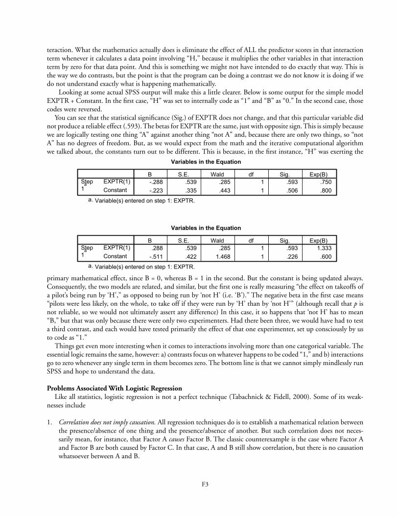
Looking at some actual SPSS output will make this a little clearer. Below is some output for the simple model EXPTR + Constant. In the first case, “H” was set to internally code as “1” and “B” as “0.” In the second case, those codes were reversed.

You can see that the statistical significance (Sig.) of EXPTR does not change, and that this particular variable did not produce a reliable effect (.593). The betas for EXPTR are the same, just with opposite sign. This is simply because we are logically testing one thing “A” against another thing “not A” and, because there are only two things, so “not A” has no degrees of freedom. But, as we would expect from the math and the iterative computational algorithm we talked about, the constants turn out to be different. This is because, in the first instance, “H” was exerting the

primary mathematical effect, since B = 0, whereas B = 1 in the second. But the constant is being updated always. Consequently, the two models are related, and similar, but the first one is really measuring “the effect on takeoffs of a pilot’s being run by ‘H’,” as opposed to being run by ‘not H’ (i.e. ‘B’).” The negative beta in the first case means “pilots were less likely, on the whole, to take off if they were run by ‘H’ than by ‘not H’” (although recall that p is not reliable, so we would not ultimately assert any difference) In this case, it so happens that ‘not H’ has to mean “B,” but that was only because there were only two experimenters. Had there been three, we would have had to test a third contrast, and each would have tested primarily the effect of that one experimenter, set up consciously by us to code as “1.”

Things get even more interesting when it comes to interactions involving more than one categorical variable. The essential logic remains the same, however: a) contrasts focus on whatever happens to be coded “1,” and b) interactions go to zero whenever any single term in them becomes zero. The bottom line is that we cannot simply mindlessly run SPSS and hope to understand the data.

Problems Associated With Logistic RegressionLike all statistics, logistic regression is not a perfect technique (Tabachnick & Fidell, 2000). Some of its weak-

nesses include

1. Correlation does not imply causation. All regression techniques do is to establish a mathematical relation between the presence/absence of one thing and the presence/absence of another. But such correlation does not neces-sarily mean, for instance, that Factor A causes Factor B. The classic counterexample is the case where Factor A and Factor B are both caused by Factor C. In that case, A and B still show correlation, but there is no causation whatsoever between A and B.


-.288 .539 .285 1 .593 .750-.223 .335 .443 1 .506 .800

EXPTR(1)Constant

Step1

a


Variable(s) entered on step 1: EXPTR.a.


.288 .539 .285 1 .593 1.333-.511 .422 1.468 1 .226 .600

EXPTR(1)Constant

Step1

a


Variable(s) entered on step 1: EXPTR.a.

F4 F5

2. Outliers can greatly skew models and parameter estimates. We demonstrated this clearly in Appendix E. Fortunately, this problem was easily overcome by winsorizing the data.

3. Independence of samples is assumed. Logistic regression is basically a between-subjects technique, not for repeated measures gathered over time. That was not a factor in this study, however.

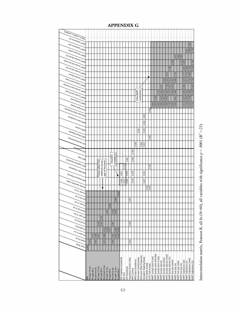
4. Absence of multicollinearity is assumed. If predictors are highly correlated, they are probably measuring the same factor, and will not contribute much, if anything additional to a model, other than wrongly inflated significance. Fortunately, the models we present did not pose this problem (see Appendix G for the intercorrelation matri-ces).

5. The ratio of cases to model predictors is important. A common rule of thumb, seen in many textbooks, is that a model should contain no more than one predictor per 10 cases (e.g., per 10 pilots). If a constant is used, this should be counted as one predictor However, we noticed an ancillary problem during this analysis, namely

6. The case-to-predictor ratio issue extends to the number of predictors measured before analysis is commenced. This is discussed in greater depth below, and in the Part II report.

Problems Associated With Too Many Predictors in Forward Stepwise Logistic RegressionAt some point, we had the intuition that simply trying to examine too many predictors in our primary technique

of forward stepwise regression could introduce a combinatorial problem. That theoretical problem is easiest illustrated using our actual situation. We started with 83 candidate predictors, some of which were eventually eliminated due to reasons such as having missing values or being discrete (which often led to unwieldy combinations of contrasts). So, in the end, we looked at roughly 60 predictors.

Now, consider the following deductive logic: Suppose you were trying to model some data taken from 30 pilots, upon whom you had 60 measurements (predictors) each. This would correspond to, say, our Low Financial Incentive group. Then the rule of thumb we mentioned above in Point 5 suggests that all such models should have no more than 30/10 = 3 predictors. So far, so good.

The problem comes when we consider random numbers. Suppose every one of our predictors was simply “noise,” taken randomly from a Gaussian (normal, bell-shaped) distribution of numbers. Given that the logistic regression prediction equation is basically

(1)

notice how the exponent term –((β0 +) β

1X

1...) is really a sum. It will be the sum of our predictors (each weighted).

That means that, whatever the actual numbers are for each pilot’s predictor scores, we are going to weight them, then add them up to form a total, which will then be plugged into Eq. 1. So what are the chances that, given noth-ing but random numbers, SPSS will ultimately end up finding the precise set of β weights such that the Equation 1 turns out greater than 0.5 for pilots who subsequently took off, versus a predicted score of less than 0.5 for those who did not?

Shockingly, the answer is that it is highly likely. We verified this by running Monte Carlo simulations, a standard technique in statistics. Using normal random number generation with µ (mu, mean) of 5 and σ (sigma, standard deviation) of 1, we were easily able to duplicate results such as the following:

This illustrates that SPSS essentially “made sense out of nonsense.” It summed the three random pseudo-predictor scores for each pilot, shown by the three jagged curves, multiplying each score by the β weights it derived, inserted them into Equation 1 and came up with the much-more regular solid “Prediction Equation” line. Notice how closely that matched the thick, dashed “Takeoff” line representing a dependent variable score of 1 for a takeoff and 0 for a non-takeoff. The three points where those two curves did not closely correspond are labeled as “error.” Since 27 of the 30 cases were “predicted” correctly, this model’s predictivity was .90.

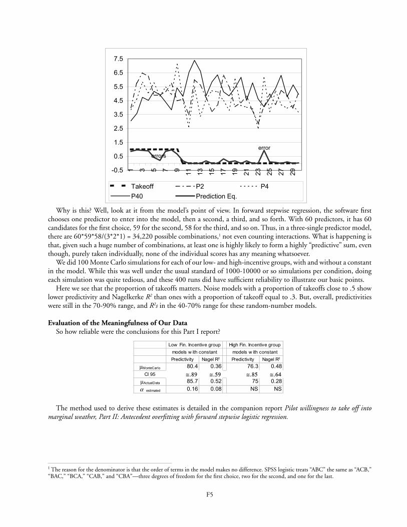
F4 F5

Why is this? Well, look at it from the model’s point of view. In forward stepwise regression, the software first chooses one predictor to enter into the model, then a second, a third, and so forth. With 60 predictors, it has 60 candidates for the first choice, 59 for the second, 58 for the third, and so on. Thus, in a three-single predictor model, there are 60*59*58/(3*2*1) = 34,220 possible combinations,1 not even counting interactions. What is happening is that, given such a huge number of combinations, at least one is highly likely to form a highly “predictive” sum, even though, purely taken individually, none of the individual scores has any meaning whatsoever.

We did 100 Monte Carlo simulations for each of our low- and high-incentive groups, with and without a constant in the model. While this was well under the usual standard of 1000-10000 or so simulations per condition, doing each simulation was quite tedious, and these 400 runs did have sufficient reliability to illustrate our basic points.

Here we see that the proportion of takeoffs matters. Noise models with a proportion of takeoffs close to .5 show lower predictivity and Nagelkerke R2 than ones with a proportion of takeoff equal to .3. But, overall, predictivities were still in the 70-90% range, and R2s in the 40-70% range for these random-number models.

Evaluation of the Meaningfulness of Our DataSo how reliable were the conclusions for this Part I report?

The method used to derive these estimates is detailed in the companion report Pilot willingness to take off into marginal weather, Part II: Antecedent overfitting with forward stepwise logistic regression.

-0.5

0.5

1.5

2.5

3.5

4.5

5.5

6.5

7.5

1 3 5 7 9 11 13 15 17 19 21 23 25 27 29

Takeoff P2 P4P40 Prediction Eq.

errorerrors

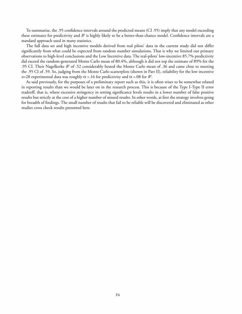
Low Fin. Incentive group High Fin. Incentive groupmodels w ith constant models w ith constantPredictivity Nagel R2 Predictivity Nagel R2

�MonteCarlo 80.4 0.36 76.3 0.48CI .95 ��

�ActualData 85.7 0.52 75 0.28� estimated 0.16 0.08 NS NS

1 The reason for the denominator is that the order of terms in the model makes no difference. SPSS logistic treats “ABC” the same as “ACB,” “BAC,” “BCA,” “CAB,” and “CBA”—three degrees of freedom for the first choice, two for the second, and one for the last.

F6 G1

To summarize, the .95 confidence intervals around the predicted means (CI .95) imply that any model exceeding these estimates for predictivity and R2 is highly likely to be a better-than-chance model. Confidence intervals are a standard approach used in many statistics.

The full data set and high incentive models derived from real pilots’ data in the current study did not differ significantly from what could be expected from random number simulations. That is why we limited our primary observations to high-level conclusions and the Low Incentive data. The real-pilots’ low-incentive 85.7% predictivity did exceed the random-generated Monte Carlo mean of 80.4%, although it did not top the estimate of 89% for the .95 CI. Their Nagelkerke R2 of .52 considerably bested the Monte Carlo mean of .36 and came close to meeting the .95 CI of .59. So, judging from the Monte Carlo scatterplots (shown in Part II), reliability for the low incentive n=28 experimental data was roughly α =.16 for predictivity and α =.08 for R2.

As said previously, for the purposes of a preliminary report such as this, it is often wiser to be somewhat relaxed in reporting results than we would be later on in the research process. This is because of the Type I-Type II error tradeoff, that is, where excessive stringency in setting significance levels results in a lower number of false positive results but strictly at the cost of a higher number of missed results. In other words, at first the strategy involves going for breadth of findings. The small number of results that fail to be reliable will be discovered and eliminated as other studies cross check results presented here.

F6 G1

APPENDIX G

YearsflyingFlighthrstotFHpast12moFHpast90dHiperfhrstotHPpast12moSimdinstrhrtotSIpast12moActinsthrtotAIpast12moAnxietySensitivityIndex BISImpulsivePlanningBISMotorImpulsivityBISCognitiveImpulsivity BISTotal

EISImpulsivity

Age

0.68

6FH

pas

t 12

mo

0.61

9FH

pas

t 90

d0.

737

Hi p

erf h

rs to

t0.

591

0.48

2H

P p

ast 1

2 m

o0.

631

0.74

4H

P p

ast 9

0 d

0.54

10.

767

Sim

d in

str h

r tot

0.67

30.

686

0.61

2S

I pas

t 12

mo

0.52

00.

567

SI p

ast 9

0 d

0.51

70.

828

Act

inst

hr t

ot0.

904

0.48

10.

581

0.64

2A

I pas

t 12

mo

0.69

30.

656

0.55

90.

500

AI p

ast 9

0 d

0.62

30.

605

0.91

5B

IS C

ogni

tive

Impu

lsiv

ity0.

560

0.60

1B

IS (t

ot)

0.81

50.

775

EIS

Impu

lsiv

ity0.

558

0.57

80.

488

Haz

ardo

us E

vent

s In

dex

0.60

40.

508

0.59

7M

PQ

Con

trol

-0.5

76-0

.576

-0.4

88-0

.766

MP

Q H

arm

Avo

idan

ceR

ohrm

ann

Cau

tious

ness

Roh

rman

n R

isk

Pro

pens

ityS

ensa

tion

See

king

Sca

le0.

487

0.53

2S

TAI S

tate

Anx

iety

0.53

2S

TAI T

rait

Anx

iety

0.58

70.

578

BAR

T pu

mps

(ave

lo p

ay)

BA

RT

pum

ps (a

ve m

ed p

ay)

BAR

T pu

mps

(ave

hi p

ay)

BA

RT

pum

ps a

dj a

veB

AR

T pu

mps

adj

ave

(lo)

BA

RT

pum

ps a

dj a

ve (m

ed)

BA

RT

pum

ps a

dj a

ve (h

i)B

AR

T av

e pa

y (c

ents

)B

AR

T av

e pa

y (lo

)B

AR

T av

e pa

y (m

ed)

BA

RT

ave

pay

(hi)

BA

RT

expl

osio

ns (t

ot)

BA

RT

expl

osio

ns (l

o)B

AR

T ex

plos

ions

(med

)B

AR

T ex

plos

ions

(hi)

Thes

e re

flect

the

rela

tivel

y yo

ung

age

of th

e pi

lots

Intra

-BIS

co

rrel

atio

ns

sivity

EISVenturesomeness MPQStressReaction MPQControl

MPQHarmAvoidance RohrmannRiskPropensity STAIStateAnxiety BARTpumps(ave) BARTpumps(avelopay) BARTpumps(avemedpay)BARTpumps(avehipay) BARTpumpsadjave BARTpumpsadjave(lo) BARTpumpsadjave(med)BARTpumpsadjave(hi) BARTavepay(cents) BARTexplosions(tot) BARTexplosions(lo) Waldp(modelw.constant)

-0.5

670.

532

0.56

20.

647

-0.5

20-0

.484

0.49

3

0.64

80.

669

0.84

50.

937

0.72

50.

829

0.73

20.

982

0.81

00.

924

0.83

10.

822

0.96

70.

707

0.81

80.

908

0.67

90.

964

0.74

00.

930

0.67

30.

793

0.70

10.

977

0.81

30.

726

0.55

40.

523

0.57

40.

576

0.53

80.

528

0.58

10.

496

0.58

00.

712

0.67

20.

805

0.51

20.

697

0.91

30.

837

0.85

80.

684

0.87

90.

777

0.84

40.

655

0.74

90.

878

0.62

30.

677

0.77

50.

568

0.84

10.

761

0.72

90.

789

0.74

40.

693

0.75

50.

890

0.68

10.

753

0.70

50.

832

0.75

90.

769

0.78

00.

735

Intra

-BAR

T co

rrel

atio

ns

Inte

rcor

rela

tion

mat

rix, P

ears

on R

, all

Ss (N

=60)

, all

varia

bles

with

sign

ifica

nce p

< .0

001

(R2 >

.23)

.

G2 G3

0.01

Thre

shol

d si

gnifi

canc

e (p

<�) 2

-taile

d

Yearsflying

Age

Flighthrstotal

FHpast12monthsFHpast90daysHiperfhrstot

HPpast12mo

HPpast90d

SimdinstrhrtotSIpast12mo

SIpast90d

Actinsthrtot

AIpast12mo

ASA

ASI

BISImpulsivePlanningBISMotorImpulsivityBISCognitiveImpulsivity EISImpulsivity

EISVenturesomenessEISEmpathy

MPQStressReactionMPQAlienationMPQControl

0.71

80.

480

0.70

20.

753

0.52

40.

616

0.63

10.

685

0.49

90.

850

0.69

60.

587

0.60

20.

768

0.61

30.

575

0.53

20.

682

0.79

10.

479

0.51

60.

481

0.84

10.

914

0.71

40.

615

0.61

60.

727

0.87

30.

730

0.80

80.

487

0.61

80.

561

0.62

50.

668

0.49

90.

662

0.72

70.

501

0.53

90.

696

0.87

3-0

.535

0.51

1

0.48

80.

676

0.75

30.

697

0.47

80.

660

0.51

5-0

.533

0.46

9

0.56

60.

494

-0.4

640.

537

0.50

80.

504

0.48

3

0.46

8

0.48

50.

476

0.47

2-0

.576

-0.6

48-0

.470

-0.7

82-0

.464

-0.6

21

0.47

30.

676

0.53

00.

522

0.68

2-0

.490

0.48

40.

470

0.49

60.

561

0.48

50.

661

0.53

1

-0.4

66

-0.5

10

-0.4

97

-0.4

83

MPQHarmAvoidanceSTAIStateAnxietySTAITraitAnxietyBARTduration(sec.)BARTpumps(ave.)BARTpumps(ave.lowpayoff) BARTpumps(ave.med.payoff) BARTpumps(ave.highpayoff) BARTpumpsadjustedave. BARTpumpsadj.ave.(low) BARTpumpsadj.ave.(med) BARTpumpsadj.ave.(high) BARTave.payoff(cents) BARTballoonexplosions(total) BARTexplosions(lowsched) BARTexplosions(med) Ye

ars

flyin

gA

geFl

ight

hrs

tot

FH p

ast 1

2 m

oFH

pas

t 90

dH

i per

f hrs

tot

HP

pas

t 12

mo

HP

pas

t 90

dS

imd

inst

r hr t

otS

I pas

t 12

mo

SI p

ast 9

0 d

Act

inst

hr t

otA

I pas

t 12

mo

AI p

ast 9

0 d

AS

A A

viat

ion

Saf

ety

Atti

tude

Sca

leA

SI A

nxie

ty S

ensi

tivity

Inde

x,B

IS Im

puls

ive

Pla

nnin

gB

IS M

otor

Impu

lsiv

ity

BIS

Cog

nitiv

e Im

puls

ivity

Bar

ratt

Impu

lsiv

enes

s S

cale

tota

lE

ysen

ck Im

puls

ivity

Sca

le Im

puls

ivity

EIS

Ven

ture

som

enes

sE

IS E

mpa

thy

HE

I Haz

ardo

us E

vent

s In

dex

MP

Q W

ellb

eing

MP

Q S

ocia

l Pot

ency

MP

Q A

chie

vem

ent

MP

Q S

ocia

l Clo

sene

ssM

PQ

Stre

ss R

eact

ion

MP

Q A

liena

tion

MP

Q A

ggre

ssio

nM

PQ

Con

trol

MP

Q H

arm

Avo

idan

ceM

PQ

Tra

ditio

nalis

mM

PQ

Abs

orpt

ion

Roh

rman

n C

autio

usne

ssR

ohrm

ann

Ris

k P

rope

nsity

-0.5

65S

SS

Sen

satio

n S

eeki

ng S

cale

STA

I Sta

te A

nxie

ty0.

740

STA

I Tra

it A

nxie

tyB

AR

T du

ratio

n (s

econ

ds)

0.46

3B

AR

T pu

mps

(ave

rage

)0.

467

0.82

5B

AR

T pu

mps

(ave

. low

pay

sche

d)0.

934

0.64

8B

AR

T pu

mps

(ave

. med

. pay

off)

0.87

50.

494

0.82

9B

AR

T pu

mps

(ave

. hig

h pa

yoff)

0.48

70.

981

0.77

80.

930

0.88

0B

AR

T pu

mps

adj

uste

d av

e.0.

515

0.80

00.

959

0.64

30.

476

0.78

6B

AR

T pu

mps

adj

uste

d av

e.(lo

w)

0.88

90.

579

0.95

60.

825

0.92

40.

582

BA

RT

pum

ps a

djus

ted

ave.

(med

)0.

842

0.80

90.

968

0.87

50.

831

BA

RT

pum

ps a

djus

ted

ave.

(hig

h)B

AR

T av

e. p

ayof

f ear

ned

(cen

ts)

0.48

90.

498

0.50

20.

471

0.54

40.

672

0.74

3B

AR

T av

e. p

ayof

f (lo

w s

ched

ule)

0.46

90.

800

BA

RT

ave.

pay

off (

med

)0.

750

BA

RT

ave.

pay

off (

high

)0.

919

0.81

50.

859

0.74

10.

890

0.73

70.

843

0.72

1B

AR

T ba

lloon

exp

losi

ons

(tota

l)0.

705

0.90

00.

508

0.62

80.

788

0.80

8B

AR

T ex

plos

ions

(low

sch

ed)

0.79

30.

692

0.83

50.

564

0.79

10.

653

0.80

30.

585

0.89

90.

630

BA

RT

expl

osio

ns (m

ed)

0.79

70.

793

0.88

30.

801

0.85

10.

839

0.78

60.

585

BA

RT

expl

osio

ns (h

igh)

Inte

rcor

rela

tion

mat

rix, P

ears

on R

, all

varia

bles

with

sign

ifica

nce p

< .0

1, L

ow F

inan

cial

Ince

ntiv

e gr

oup

(N=3

0).

G2 G3

Yearsflying

Flighthrstot

FHpast12mo

FHpast90d

Hiperfhrstot

HPpast12mo

HPpast90d

SimdinstrhrtotSIpast12mo

Actinsthrtot

AIpast12mo

BISImpulsivePlanning BISMotorImpulsivityBISCognitiveImpulsivity BarrattImpulsivenessScaletotalEISImpulsivity

EISVenturesomenessMPQStressReactionMPQControl

0.71

80.

702

0.75

30.

685

0.85

00.

696

0.76

80.

682

0.79

10.

841

0.91

40.

714

0.72

70.

873

0.73

00.

808

0.66

80.

662

0.72

70.

696

0.87

30.

676

0.69

70.

753

0.69

70.

660

-0.7

820.

676

0.68

20.

661

Intra

-BAR

Tco

rrel

atio

ns

Thes

e R

s re

flect

the

rela

tivel

yyo

ung

med

ian

age

of th

e pi

lots

Intra

-BIS

corr

elat

ions

trol

STAIStateAnxietyBARTpumps(ave.)BARTpumps(ave.lowpayoff) BARTpumps(ave.med.payoff) BARTpumps(ave.highpayoff) BARTpumpsadjustedave. BARTpumpsadj.ave.(low) BARTpumpsadj.ave.(med) BARTpumpsadj.ave.(high) BARTave.payoff(cents) BARTballoonexplosions(total) C

orrelations

(N=3

0 in

all

case

s)Ag

eFH

pas

t 12

mo

FH p

ast 9

0 d

HP

past

12

mo

HP

past

90

dSi

md

inst

r hr t

otSI

pas

t 90

dAc

t ins

t hr t

otAI

pas

t 12

mo

AI p

ast 9

0 d

BIS

Cog

nitiv

e Im

puls

ivity

Barra

tt Im

puls

iven

ess

Scal

e to

tal

Eyse

nck

Impu

lsiv

ity S

cale

Impu

lsiv

ityM

PQ

Con

trol

Roh

rman

n C

autio

usne

ssSS

S S

ensa

tion

Seek

ing

Scal

e0.

740

STAI

Tra

it An

xiet

y0.

825

BAR

T pu

mps

(ave

. low

pay

off s

ched

)0.

934

BAR

T pu

mps

(ave

. med

. pay

off)

0.87

50.

829

BAR

T pu

mps

(ave

. hig

h pa

yoff)

0.98

10.

778

0.93

00.

880

BAR

T pu

mps

adj

uste

d av

e.0.

800

0.95

90.

786

BAR

T pu

mps

adj

uste

d av

e.(lo

w)

0.88

90.

956

0.82

50.

924

BAR

T pu

mps

adj

uste

d av

e.(m

ed)

0.84

20.

809

0.96

80.

875

0.83

1BA

RT

pum

ps a

djus

ted

ave.

(hig

h)0.

672

0.74

3BA

RT

ave.

pay

off (

low

sch

edul

e)0.

800

BAR

T av

e. p

ayof

f (m

ed)

0.75

0BA

RT

ave.

pay

off (

high

)0.

919

0.81

50.

859

0.74

10.

890

0.73

70.

843

0.72

1BA

RT

ballo

on e

xplo

sion

s (to

tal)

0.70

50.

900

0.78

80.

808

BAR

T ba

lloon

exp

losi

ons

(low

sch

ed)

0.79

30.

692

0.83

50.

791

0.65

30.

803

0.89

9BA

RT

ballo

on e

xplo

sion

s (m

ed)

0.79

70.

793

0.88

30.

801

0.85

10.

839

0.78

6BA

RT

ballo

on e

xplo

sion

s (h

igh)

Inte

rcor

rela

tion

mat

rix, P

ears

on R

, all

varia

bles

with

sign

ifica

nce p

< .0

001

(equ

ival

ent t

o R

2 > .4

4), L

ow F

inan

cial

Ince

ntiv

e gr

oup

(N=3

0). N

ote

that

mos

t of

the

high

ly si

gnifi

cant

cor

rela

tions

hav

e ve

ry si

mpl

e ex

plan

atio

ns

G4 H1

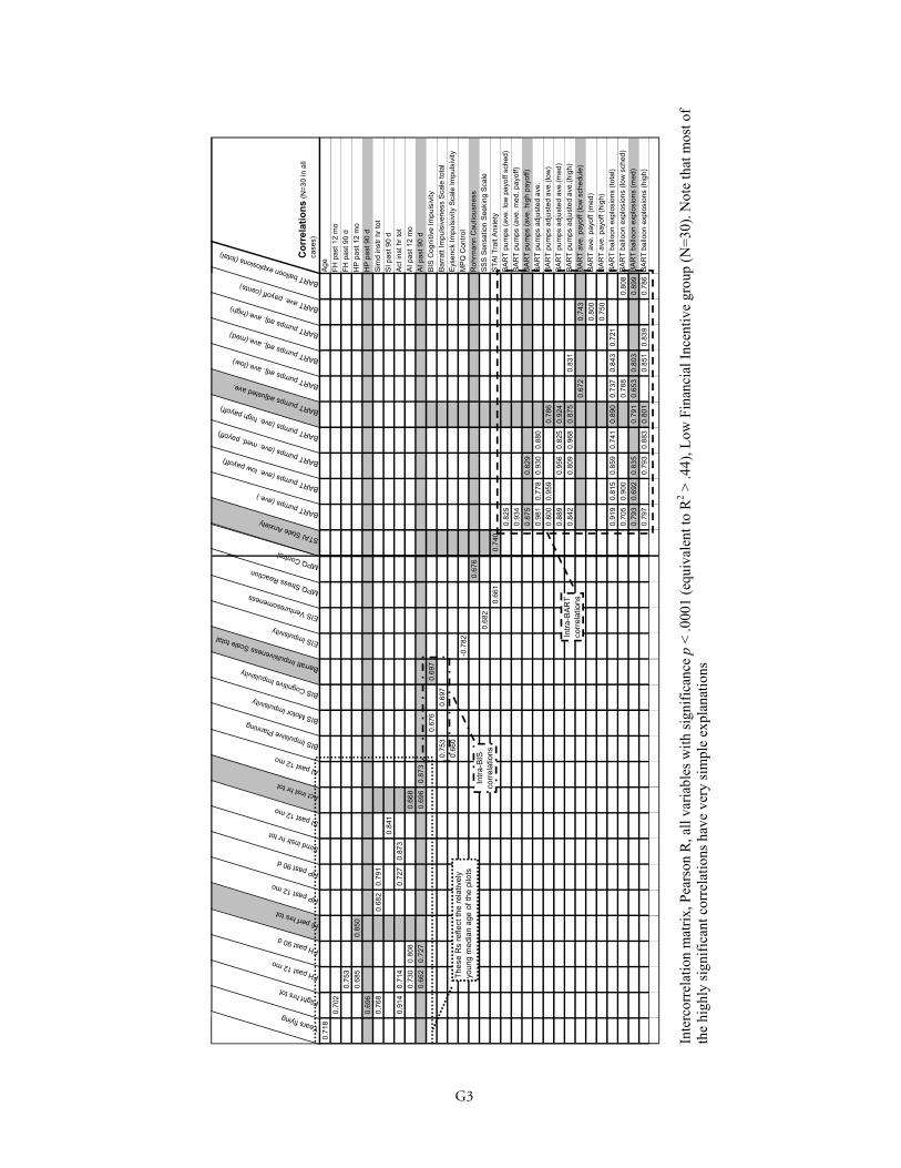
Pearson Rs, variables with significance p < .0001 (equivalent to .44 ≤ R2 ≤ .61) whose explanation is not obvi-ous simply because they are correlated by their very nature (e.g. the various measures calculated from BART). The upshot here is that a) Each of these correlations is perfectly logical, and; b) Even this small number of correlations involves less than half the variance. That means that each instrument presumably measured different factors for the most fact, which was as it should be.

BIS

Impu

lsiv

ePl

anni

ngEI

SIm

puls

ivity

EIS

Vent

ures

omen

ess

MPQ

Stre

ssR

eact

ion

MPQ

Con

trol

STAI

Stat

eAn

xiet

y

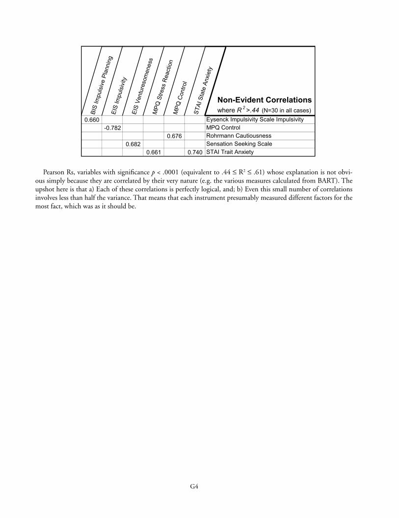
Non-Evident Correlations where R 2 >.44 (N=30 in all cases)

0.660 Eysenck Impulsivity Scale Impulsivity-0.782 MPQ Control

0.676 Rohrmann Cautiousness0.682 Sensation Seeking Scale

0.661 0.740 STAI Trait Anxiety

G4 H1

APPENDIX H

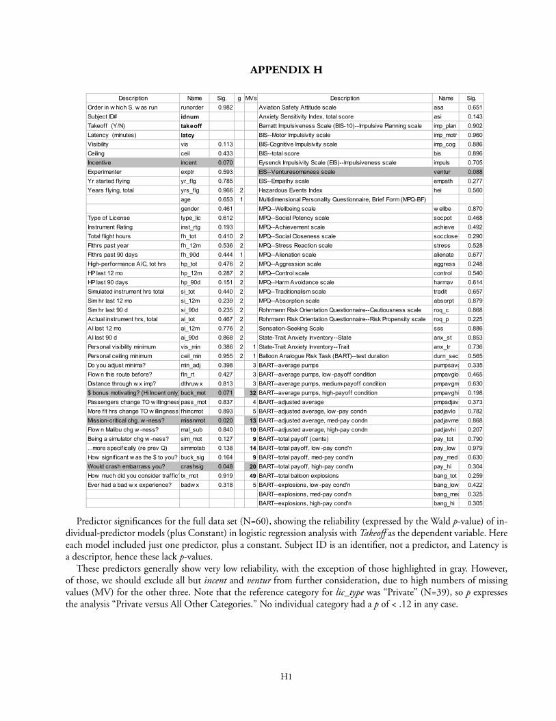
Predictor significances for the full data set (N=60), showing the reliability (expressed by the Wald p-value) of in-dividual-predictor models (plus Constant) in logistic regression analysis with Takeoff as the dependent variable. Here each model included just one predictor, plus a constant. Subject ID is an identifier, not a predictor, and Latency is a descriptor, hence these lack p-values.

These predictors generally show very low reliability, with the exception of those highlighted in gray. However, of those, we should exclude all but incent and ventur from further consideration, due to high numbers of missing values (MV) for the other three. Note that the reference category for lic_type was “Private” (N=39), so p expresses the analysis “Private versus All Other Categories.” No individual category had a p of < .12 in any case.

Description Name Sig. g MVs Description Name Sig.Order in w hich S. w as run runorder 0.982 Aviation Safety Attitude scale asa 0.651Subject ID# idnum Anxiety Sensitivity Index, total score asi 0.143Takeoff (Y/N) takeoff Barratt Impulsiveness Scale (BIS-10)--Impulsive Planning scale imp_plan 0.902Latency (minutes) latcy BIS--Motor Impulsivity scale imp_motr 0.960Visibility vis 0.113 BIS-Cognitive Impulsivity scale imp_cog 0.886Ceiling ceil 0.433 BIS--total score bis 0.896Incentive incent 0.070 Eysenck Impulsivity Scale (EIS)--Impulsiveness scale impuls 0.705Experimenter exptr 0.593 EIS--Venturesomeness scale ventur 0.088Yr started f lying yr_flg 0.785 EIS--Empathy scale empath 0.277Years f lying, total yrs_flg 0.966 2 Hazardous Events Index hei 0.560

age 0.653 1 Multidimensional Personality Questionnaire, Brief Form (MPQ-BF)gender 0.461 MPQ--Wellbeing scale w ellbe 0.870

Type of License type_lic 0.612 MPQ--Social Potency scale socpot 0.468Instrument Rating inst_rtg 0.193 MPQ--Achievement scale achieve 0.492Total f light hours fh_tot 0.410 2 MPQ--Social Closeness scale socclose 0.290Flthrs past year fh_12m 0.536 2 MPQ--Stress Reaction scale stress 0.528Flthrs past 90 days fh_90d 0.444 1 MPQ--Alienation scale alienate 0.677High-performance A/C, tot hrs hp_tot 0.476 2 MPQ--Aggression scale aggress 0.248HP last 12 mo hp_12m 0.287 2 MPQ--Control scale control 0.540HP last 90 days hp_90d 0.151 2 MPQ--Harm Avoidance scale harmav 0.614Simulated instrument hrs total si_tot 0.440 2 MPQ--Traditionalism scale tradit 0.657Sim hr last 12 mo si_12m 0.239 2 MPQ--Absorption scale absorpt 0.879Sim hr last 90 d si_90d 0.235 2 Rohrmann Risk Orientation Questionnaire--Cautiousness scale roq_c 0.868Actual instrument hrs, total ai_tot 0.467 2 Rohrmann Risk Orientation Questionnaire--Risk Propensity scale roq_p 0.225AI last 12 mo ai_12m 0.776 2 Sensation-Seeking Scale sss 0.886AI last 90 d ai_90d 0.868 2 State-Trait Anxiety Inventory--State anx_st 0.853Personal visibility minimum vis_min 0.386 2 1 State-Trait Anxiety Inventory--Trait anx_tr 0.736Personal ceiling minimum ceil_min 0.955 2 1 Balloon Analogue Risk Task (BART)--test duration durn_sec 0.565Do you adjust minima? min_adj 0.398 3 BART--average pumps pumpsavg 0.335Flow n this route before? fln_rt 0.427 3 BART--average pumps, low -payoff condition pmpavglo 0.465Distance through w x imp? dthruw x 0.813 3 BART--average pumps, medium-payoff condition pmpavgm 0.630$ bonus motivating? (Hi Incent only)buck_mot 0.071 32 BART--average pumps, high-payoff condition pmpavghi 0.198Passengers change TO w illingness pass_mot 0.837 4 BART--adjusted average pmpadjav 0.373More flt hrs change TO w illingness?fhincmot 0.893 5 BART--adjusted average, low -pay condn padjavlo 0.782Mission-critical chg. w -ness? missnmot 0.020 13 BART--adjusted average, med-pay condn padjavme 0.868Flow n Malibu chg w -ness? mal_sub 0.840 10 BART--adjusted average, high-pay condn padjavhi 0.207Being a simulator chg w -ness? sim_mot 0.127 9 BART--total payoff (cents) pay_tot 0.790...more specif ically (re prev Q) simmotsb 0.138 14 BART--total payoff, low -pay cond'n pay_low 0.979How signif icant w as the $ to you? buck_sig 0.164 9 BART--total payoff, med-pay cond'n pay_med 0.630Would crash embarrass you? crashsig 0.048 20 BART--total payoff, high-pay cond'n pay_hi 0.304How much did you consider traff ic?tx_mot 0.919 49 BART--total balloon explosions bang_tot 0.259Ever had a bad w x experience? badw x 0.318 5 BART--explosions, low -pay cond'n bang_low 0.422

BART--explosions, med-pay cond'n bang_med 0.325BART--explosions, high-pay cond'n bang_hi 0.305

I1

Description Name Sig. g MVs Description Name Sig.Order in w hich S. w as run runorder 0.675 Aviation Safety Attitude scale asa 0.645Subject ID# idnum Anxiety Sensitivity Index, total score asi 0.127Takeoff (Y/N) takeoff Barratt Impulsiveness Scale (BIS-10)--Impulsive Planning scale imp_plan 0.615Latency (minutes) latcy BIS--Motor Impulsivity scale imp_motr 0.957Visibility vis 0.064 BIS-Cognitive Impulsivity scale imp_cog 0.398Ceiling ceil 0.691 BIS--total score bis 0.562Incentive incent Eysenck Impulsivity Scale (EIS)--Impulsiveness scale impuls 0.394Experimenter exptr 0.261 EIS--Venturesomeness scale ventur 0.713Yr started f lying yr_flg EIS--Empathy scale empath 0.881Years f lying, total yrs_flg 0.470 2 Hazardous Events Index hei 0.221

age 0.942 1 Multidimensional Personality Questionnaire, Brief Form (MPQ-BF)gender 0.815 MPQ--Wellbeing scale w ellbe 0.896

Type of License type_lic 0.999 MPQ--Social Potency scale socpot 0.269Instrument Rating inst_rtg 0.873 MPQ--Achievement scale achieve 0.574Total f light hours fh_tot 0.591 1 MPQ--Social Closeness scale socclose 0.590Flthrs past year fh_12m 0.911 2 MPQ--Stress Reaction scale stress 0.544Flthrs past 90 days fh_90d 0.907 MPQ--Alienation scale alienate 0.787High-performance A/C, tot hrs hp_tot 0.347 2 MPQ--Aggression scale aggress 0.673HP last 12 mo hp_12m 0.713 2 MPQ--Control scale control 0.930HP last 90 days hp_90d 0.328 2 MPQ--Harm Avoidance scale harmav 0.641Simulated instrument hrs total si_tot 0.995 MPQ--Traditionalism scale tradit 0.203Sim hr last 12 mo si_12m 0.588 2 MPQ--Absorption scale absorpt 0.961Sim hr last 90 d si_90d 0.982 2 Rohrmann Risk Orientation Questionnaire--Cautiousness scale roq_c 0.345Actual instrument hrs, total ai_tot 0.482 2 Rohrmann Risk Orientation Questionnaire--Risk Propensity scale roq_p 0.637AI last 12 mo ai_12m 0.753 1 Sensation-Seeking Scale sss 0.888AI last 90 d ai_90d 0.512 1 State-Trait Anxiety Inventory--State anx_st 0.484Personal visibility minimum vis_min 0.523 State-Trait Anxiety Inventory--Trait anx_tr 0.393Personal ceiling minimum ceil_min 0.487 1 Balloon Analogue Risk Task (BART)--test duration durn_sec 0.864Do you adjust minima? min_adj 0.244 BART--average pumps pumpsav 0.341Flow n this route before? fln_rt 0.265 BART--average pumps, low -payoff condition pmpavglo 0.552Distance through w x imp? dthruw x 0.627 BART--average pumps, medium-payoff condition pmpavgm 0.462

BART--average pumps, high-payoff condition pmpavgh 0.234Passengers change TO w illingnesspass_mot 0.175 1 BART--adjusted average pmpadjav 0.460More flt hrs change TO w illingness fhincmot 0.204 BART--adjusted average, low -pay condn padjavlo 0.975Mission-critical chg. w -ness? missnmot 0.024 7 BART--adjusted average, med-pay condn padjavme 0.768Flow n Malibu chg w -ness? mal_sub 0.854 4 BART--adjusted average, high-pay condn padjavhi 0.186Being a simulator chg w -ness? sim_mot 0.910 3 BART--total payoff (cents) pay_tot 0.749...more specif ically (re prev Q) simmotsb 0.408 7 BART--total payoff, low -pay cond'n pay_low 0.836

BART--total payoff, med-pay cond'n pay_med 0.990Would crash embarrass you? crashsig 0.337 12 BART--total payoff, high-pay cond'n pay_hi 0.365How much did you consider traff ic tx_mot 0.422 26 BART--total balloon explosions bang_tot 0.272Ever had a bad w x experience? badw x 0.472 BART--explosions, low -pay cond'n bang_low 0.458

BART--explosions, med-pay cond'n bang_me 0.403BART--explosions, high-pay cond'n bang_hi 0.229

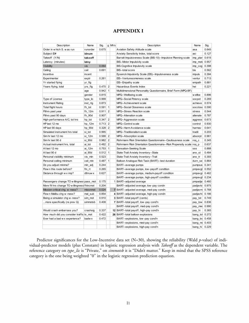
APPENDIX I

Predictor significances for the Low-Incentive data set (N=30), showing the reliability (Wald p-value) of indi-vidual-predictor models (plus Constant) in logistic regression analysis with Takeoff as the dependent variable. The reference category on type_lic is “Private,” on simmotsb it is “Didn’t matter.” Keep in mind that the SPSS reference category is the one being weighted “0” in the logistic regression prediction equation.

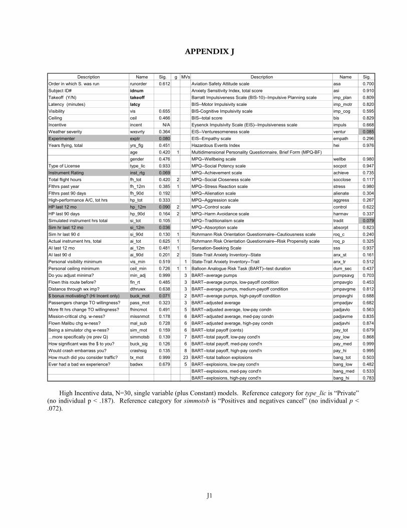
J1

APPENDIX J

Description Name Sig. g MVs Description Name Sig.Order in which S. was run runorder 0.612 Aviation Safety Attitude scale asa 0.700Subject ID# idnum Anxiety Sensitivity Index, total score asi 0.910Takeoff (Y/N) takeoff Barratt Impulsiveness Scale (BIS-10)--Impulsive Planning scale imp_plan 0.809Latency (minutes) latcy BIS--Motor Impulsivity scale imp_motr 0.820Visibility vis 0.655 BIS-Cognitive Impulsivity scale imp_cog 0.595Ceiling ceil 0.466 BIS--total score bis 0.829Incentive incent N/A Eysenck Impulsivity Scale (EIS)--Impulsiveness scale impuls 0.668Weather severity wxsvrty 0.364 EIS--Venturesomeness scale ventur 0.085Experimenter exptr 0.080 EIS--Empathy scale empath 0.296Years flying, total yrs_flg 0.451 Hazardous Events Index hei 0.976

age 0.420 1 Multidimensional Personality Questionnaire, Brief Form (MPQ-BF)gender 0.476 MPQ--Wellbeing scale wellbe 0.980

Type of License type_lic 0.933 MPQ--Social Potency scale socpot 0.947Instrument Rating inst_rtg 0.069 MPQ--Achievement scale achieve 0.735Total flight hours fh_tot 0.420 2 MPQ--Social Closeness scale socclose 0.117Flthrs past year fh_12m 0.385 1 MPQ--Stress Reaction scale stress 0.980Flthrs past 90 days fh_90d 0.192 MPQ--Alienation scale alienate 0.304High-performance A/C, tot hrs hp_tot 0.333 MPQ--Aggression scale aggress 0.267HP last 12 mo hp_12m 0.090 2 MPQ--Control scale control 0.622HP last 90 days hp_90d 0.164 2 MPQ--Harm Avoidance scale harmav 0.337Simulated instrument hrs total si_tot 0.105 MPQ--Traditionalism scale tradit 0.079Sim hr last 12 mo si_12m 0.036 MPQ--Absorption scale absorpt 0.823Sim hr last 90 d si_90d 0.130 1 Rohrmann Risk Orientation Questionnaire--Cautiousness scale roq_c 0.240Actual instrument hrs, total ai_tot 0.625 1 Rohrmann Risk Orientation Questionnaire--Risk Propensity scale roq_p 0.325AI last 12 mo ai_12m 0.481 1 Sensation-Seeking Scale sss 0.937AI last 90 d ai_90d 0.201 2 State-Trait Anxiety Inventory--State anx_st 0.161Personal visibility minimum vis_min 0.519 1 State-Trait Anxiety Inventory--Trait anx_tr 0.512Personal ceiling minimum ceil_min 0.726 1 1 Balloon Analogue Risk Task (BART)--test duration durn_sec 0.437Do you adjust minima? min_adj 0.999 3 BART--average pumps pumpsavg 0.703Flown this route before? fln_rt 0.485 3 BART--average pumps, low-payoff condition pmpavglo 0.453Distance through wx imp? dthruwx 0.638 3 BART--average pumps, medium-payoff condition pmpavgme 0.812$ bonus motivating? (Hi Incent only) buck_mot 0.071 2 BART--average pumps, high-payoff condition pmpavghi 0.688Passengers change TO willingness? pass_mot 0.323 3 BART--adjusted average pmpadjav 0.682More flt hrs change TO willingness? fhincmot 0.491 5 BART--adjusted average, low-pay condn padjavlo 0.563Mission-critical chg. w-ness? missnmot 0.178 6 BART--adjusted average, med-pay condn padjavme 0.835Flown Malibu chg w-ness? mal_sub 0.728 6 BART--adjusted average, high-pay condn padjavhi 0.874Being a simulator chg w-ness? sim_mot 0.159 6 BART--total payoff (cents) pay_tot 0.679...more specifically (re prev Q) simmotsb 0.139 7 BART--total payoff, low-pay cond'n pay_low 0.868How significant was the $ to you? buck_sig 0.126 6 BART--total payoff, med-pay cond'n pay_med 0.999Would crash embarrass you? crashsig 0.135 8 BART--total payoff, high-pay cond'n pay_hi 0.995How much did you consider traffic? tx_mot 0.999 23 BART--total balloon explosions bang_tot 0.503Ever had a bad wx experience? badwx 0.679 5 BART--explosions, low-pay cond'n bang_low 0.482

BART--explosions, med-pay cond'n bang_med 0.533BART--explosions, high-pay cond'n bang_hi 0.783

High Incentive data, N=30, single variable (plus Constant) models. Reference category for type_lic is �Private� (no individual p < .187). Reference category for simmotsb is �Positives and negatives cancel� (no individual p < .072).

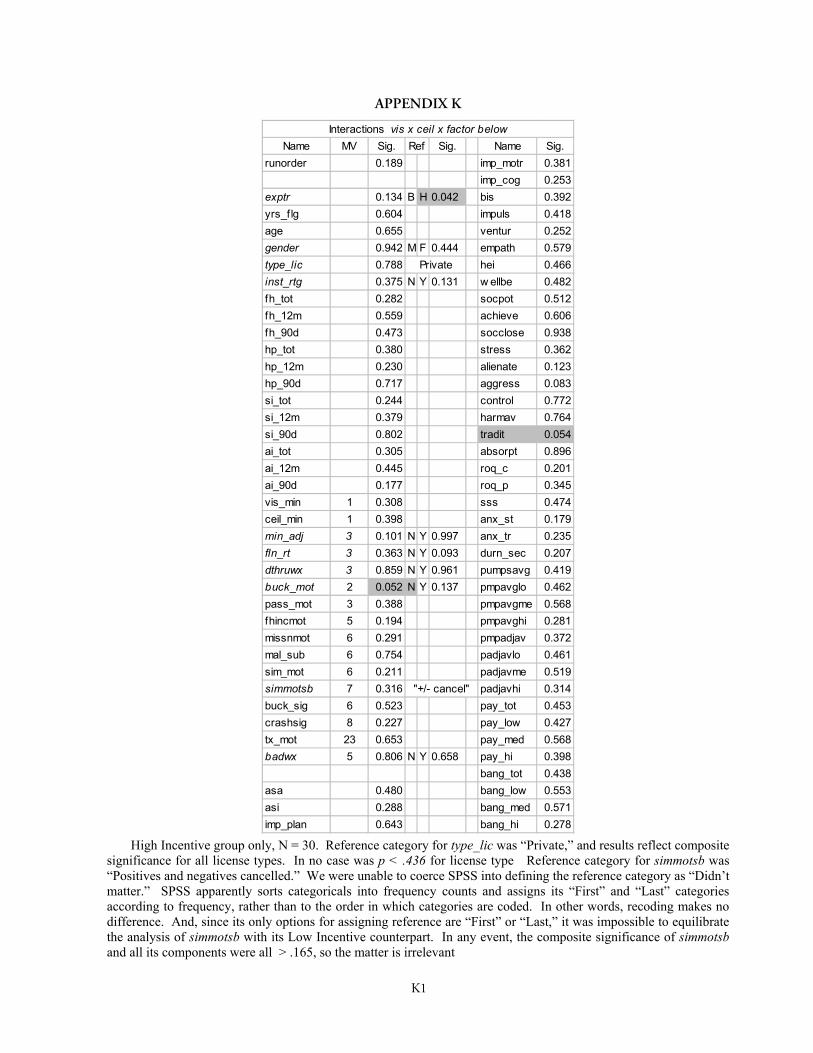
K1

��

Interactions vis x ceil x factor belowName MV Sig. Ref Sig. Name Sig.

runorder 0.189 imp_motr 0.381imp_cog 0.253

exptr 0.134 B H 0.042 bis 0.392yrs_flg 0.604 impuls 0.418age 0.655 ventur 0.252gender 0.942 M F 0.444 empath 0.579type_lic 0.788 Private hei 0.466inst_rtg 0.375 N Y 0.131 w ellbe 0.482fh_tot 0.282 socpot 0.512fh_12m 0.559 achieve 0.606fh_90d 0.473 socclose 0.938hp_tot 0.380 stress 0.362hp_12m 0.230 alienate 0.123hp_90d 0.717 aggress 0.083si_tot 0.244 control 0.772si_12m 0.379 harmav 0.764si_90d 0.802 tradit 0.054ai_tot 0.305 absorpt 0.896ai_12m 0.445 roq_c 0.201ai_90d 0.177 roq_p 0.345vis_min 1 0.308 sss 0.474ceil_min 1 0.398 anx_st 0.179min_adj 3 0.101 N Y 0.997 anx_tr 0.235fln_rt 3 0.363 N Y 0.093 durn_sec 0.207dthruwx 3 0.859 N Y 0.961 pumpsavg 0.419buck_mot 2 0.052 N Y 0.137 pmpavglo 0.462pass_mot 3 0.388 pmpavgme 0.568fhincmot 5 0.194 pmpavghi 0.281missnmot 6 0.291 pmpadjav 0.372mal_sub 6 0.754 padjavlo 0.461sim_mot 6 0.211 padjavme 0.519simmotsb 7 0.316 "+/- cancel" padjavhi 0.314buck_sig 6 0.523 pay_tot 0.453crashsig 8 0.227 pay_low 0.427tx_mot 23 0.653 pay_med 0.568badwx 5 0.806 N Y 0.658 pay_hi 0.398

bang_tot 0.438asa 0.480 bang_low 0.553asi 0.288 bang_med 0.571imp_plan 0.643 bang_hi 0.278

High Incentive group only, N = 30. Reference category for type_lic was �Private,� and results reflect composite significance for all license types. In no case was p < .436 for license type Reference category for simmotsb was �Positives and negatives cancelled.� We were unable to coerce SPSS into defining the reference category as �Didn�t matter.� SPSS apparently sorts categoricals into frequency counts and assigns its �First� and �Last� categories according to frequency, rather than to the order in which categories are coded. In other words, recoding makes no difference. And, since its only options for assigning reference are �First� or �Last,� it was impossible to equilibrate the analysis of simmotsb with its Low Incentive counterpart. In any event, the composite significance of simmotsband all its components were all > .165, so the matter is irrelevant

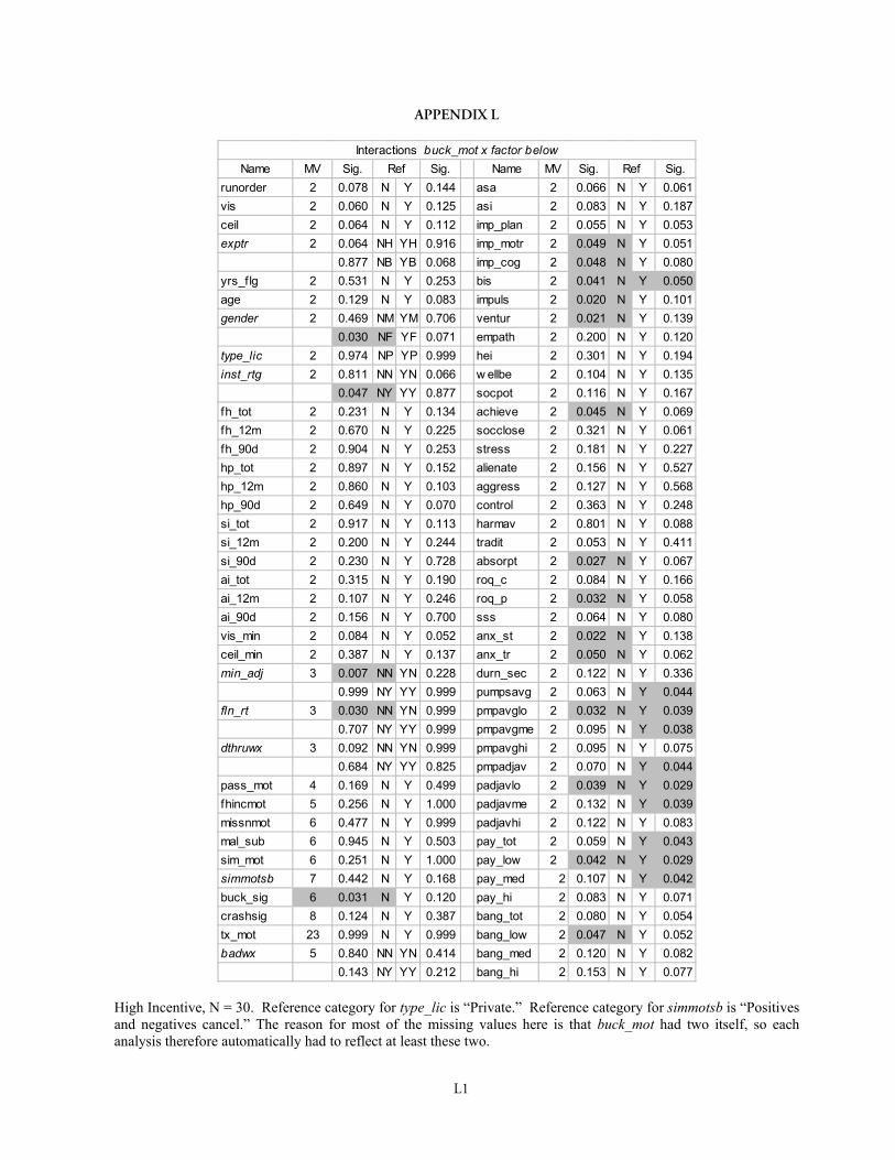
L1

��

Interactions buck_mot x factor belowName MV Sig. Ref Sig. Name MV Sig. Ref Sig.

runorder 2 0.078 N Y 0.144 asa 2 0.066 N Y 0.061vis 2 0.060 N Y 0.125 asi 2 0.083 N Y 0.187ceil 2 0.064 N Y 0.112 imp_plan 2 0.055 N Y 0.053exptr 2 0.064 NH YH 0.916 imp_motr 2 0.049 N Y 0.051

0.877 NB YB 0.068 imp_cog 2 0.048 N Y 0.080yrs_flg 2 0.531 N Y 0.253 bis 2 0.041 N Y 0.050age 2 0.129 N Y 0.083 impuls 2 0.020 N Y 0.101gender 2 0.469 NM YM 0.706 ventur 2 0.021 N Y 0.139

0.030 NF YF 0.071 empath 2 0.200 N Y 0.120type_lic 2 0.974 NP YP 0.999 hei 2 0.301 N Y 0.194inst_rtg 2 0.811 NN YN 0.066 w ellbe 2 0.104 N Y 0.135

0.047 NY YY 0.877 socpot 2 0.116 N Y 0.167fh_tot 2 0.231 N Y 0.134 achieve 2 0.045 N Y 0.069fh_12m 2 0.670 N Y 0.225 socclose 2 0.321 N Y 0.061fh_90d 2 0.904 N Y 0.253 stress 2 0.181 N Y 0.227hp_tot 2 0.897 N Y 0.152 alienate 2 0.156 N Y 0.527hp_12m 2 0.860 N Y 0.103 aggress 2 0.127 N Y 0.568hp_90d 2 0.649 N Y 0.070 control 2 0.363 N Y 0.248si_tot 2 0.917 N Y 0.113 harmav 2 0.801 N Y 0.088si_12m 2 0.200 N Y 0.244 tradit 2 0.053 N Y 0.411si_90d 2 0.230 N Y 0.728 absorpt 2 0.027 N Y 0.067ai_tot 2 0.315 N Y 0.190 roq_c 2 0.084 N Y 0.166ai_12m 2 0.107 N Y 0.246 roq_p 2 0.032 N Y 0.058ai_90d 2 0.156 N Y 0.700 sss 2 0.064 N Y 0.080vis_min 2 0.084 N Y 0.052 anx_st 2 0.022 N Y 0.138ceil_min 2 0.387 N Y 0.137 anx_tr 2 0.050 N Y 0.062min_adj 3 0.007 NN YN 0.228 durn_sec 2 0.122 N Y 0.336

0.999 NY YY 0.999 pumpsavg 2 0.063 N Y 0.044fln_rt 3 0.030 NN YN 0.999 pmpavglo 2 0.032 N Y 0.039

0.707 NY YY 0.999 pmpavgme 2 0.095 N Y 0.038dthruwx 3 0.092 NN YN 0.999 pmpavghi 2 0.095 N Y 0.075

0.684 NY YY 0.825 pmpadjav 2 0.070 N Y 0.044pass_mot 4 0.169 N Y 0.499 padjavlo 2 0.039 N Y 0.029fhincmot 5 0.256 N Y 1.000 padjavme 2 0.132 N Y 0.039missnmot 6 0.477 N Y 0.999 padjavhi 2 0.122 N Y 0.083mal_sub 6 0.945 N Y 0.503 pay_tot 2 0.059 N Y 0.043sim_mot 6 0.251 N Y 1.000 pay_low 2 0.042 N Y 0.029simmotsb 7 0.442 N Y 0.168 pay_med 2 0.107 N Y 0.042buck_sig 6 0.031 N Y 0.120 pay_hi 2 0.083 N Y 0.071crashsig 8 0.124 N Y 0.387 bang_tot 2 0.080 N Y 0.054tx_mot 23 0.999 N Y 0.999 bang_low 2 0.047 N Y 0.052badwx 5 0.840 NN YN 0.414 bang_med 2 0.120 N Y 0.082

0.143 NY YY 0.212 bang_hi 2 0.153 N Y 0.077

High Incentive, N = 30. Reference category for type_lic is �Private.� Reference category for simmotsb is �Positives and negatives cancel.� The reason for most of the missing values here is that buck_mot had two itself, so each analysis therefore automatically had to reflect at least these two.

the influence of visibility, cloud ceiling, financial ... · meaning that imc is ... yes yes yes...

Documents