the impact of the recession in the united states on the...

International Journal of Business and Social Science Vol. 4 No. 17 [Special Issue – December 2013]

110

The Impact of the Recession in the United States on the Price of US $ in Guyana

Jacqueline Murray

Department of Business and Management Studies University of Guyana, Berbice Campus

Tain, Corentyne, Guyana. Abstract

The study was undertaken to determine the impact of the recession in the United States on the spot (selling/ask) price of the United States Dollar (USD) in Guyana. The archival research method was used to gather the necessary data which was analysed using the Statistical Package for the Social Sciences version 15. Quarterly non-seasonally adjusted data for January 2006 to December 2008 (divided into pre crisis and crisis periods) of the logs of the Guyanese dollar to the United States dollar and logs of domestic and foreign variables export (Y, Y*); interest rates and money supply – M2 (M, M*) were input into a regression equation and analysed using Ordinary Least Squares. The independent variables used corresponded to those identified by the monetary model with the exception that export values were used as approximations of income. The results of the crisis period were statistically insignificant at p > .05. Indicating that supply as denoted by money supply and demand as denoted by interest did not influence the spot price of the USD during the recession. In comparison, the pre-crisis results indicated that supply as denoted by money supply had a statistically significant influence on variations in the spot price of the USD.

Key Words: Financial crisis; Exchange Rate; Demand; Supply; Contagion

1. Background to the Study

1.1 Introduction

“When America sneezes does the rest of the world have to catch cold too?” (Economist 2001). History is endemic with examples of financial crises, Mexico (1982; 1994); Finland – Exchange Rate Mechanism (ERM – 1992); Asia (1997), Russia (1998), Brazil (1999); Turkey (2001); Argentina (2001) that have impacted economically on countries regionally and/or internationally. The World Bank projected that the financial crisis, ‘credit crunch’ which began in the summer of 2007 in the United States, brought about as a result of the subprime market housing was going to hurt developing countries especially those that depend on foreign capital flows, have large current account deficits and heavy external financing needs (New York Times, 2008).

Guyana, being a small developing country whose economy relies heavily on the export of six commodities (sugar, gold, bauxite, shrimp, timber, and rice) which make up 60% of the country’s gross domestic product, might have been affected by a recession in the United States since it is a major trading partner of Guyana, gives Guyana aid and migrants there remit money home. As such a slowdown in that country’s economy might have impacted: its demand for Guyana’s exports; aid to Guyana; and the amount of United States Dollars (USD) remitted by migrants. The question which arises then is: “When America sneezed did Guyana catch a cold?

The objective of the research was to determine the impact of the recession in the United States on the spot (selling/ask) price of the United States Dollar (USD) in Guyana. The following research questions and hypotheses opertionalised the study.

1.2 Research questions

1) How has the demand for USD affected its spot ask/selling price since the recession in the United States? 2) How has the supply of USD affected its spot ask/selling price since the recession in the United States?

The Special Issue on Business, Humanities and Social Science © Center for Promoting Ideas, USA www.ijbssnet.com

111

1.3 Hypotheses

oH There is no relationship between the spot (ask) selling price of the US$ and supply since the recession

0H There is no relationship between the spot (ask) selling price of the US$ and demand since the recession

1H There is a relationship between the spot (ask) selling price of the US$ and supply since the recession

1H There is a relationship between the spot (ask) selling price of the US$ and demand since the recession

1.4 Definition of terms germane to the study

For the purpose of the study the independent variables demand and supply are generally defined in the former case as the quantity of a commodity (USD) that buyers wish to purchase per period of time at a particular price and in the latter, the quantity supplied of a commodity (USD) and its price (Lipsey and Chrystal, 1999). The dependent variable, spot (ask) selling price refers to the selling price of the foreign currency during the time of the crisis for the period investigated. Expectation, investor behaviour, and government controls are considered as intervening variables.

1.5 Associated significance of the study

There have been a number of studies done to ascertain the effect of financial cirises on economies for developed and developing countries (large) but so far none except for Pollard (2000) have addressed the effect of international disturbances on the money supply in Guyana. It is also noted that the findings of Pollard (2000) were based on statistical data derived from 1964 to 1985 and hence may not be reflective of the situation which prevailed during the initial stages of the recession. Additionally, financial contagion has been found to be transferrred almost instantaneously between countries through trade and financial related linkages, investor behaviour, and cross border capital flow, and common creditor with slow ‘spillover effect’ on other countries. This being the case , it might have been possible for a small developing country like Guyana to be advesely affected. An investigation into the effect of the recession on the price of the USD through supply and demand has potential significance: to the academic community by adding to the body of knowledge already present; to the business community for strategic planning; and to the government in future macroeconomic planing. It has been observed by Kaminsky, Reinhart, and Vegh (2003) that if history is any guide these crises will continue to occur hence the government can be proactive and institute measures to combat such an event in the future.

1.6 Limitation of Study

The researcher utilised judgement in the selection of the sample population which spanned the period January 2006 to December 2008 which confines the extent to which generalisations can be made. The researcher utilized quarterly non-seasonally adjusted data relating to the average selling price of the USD and the fundamentals (income, interest, money supply) to determine their effect on the spot price of the USD which further delimits the study. Additionally, only annual data values for income as measured by GDP were available for Guyana consequently export values were used as close approximation of income since these represent 60% of Guyana’s GDP. As a result the same measure was used as income for the United States. Monthly values which would have highlighted more variability were unavailable.

1.5 Organization of Study

The remainder of this study is organised as follows. Section 2 examines theories relating to exchange rate determination. Section 3details the methodology employed. The results of the investigation are presented in Section 4. Section 5 discusses the results and Section 6 provides the conclusions.

2. Theories of Exchange Rate Determination

2.1 Introduction

The United States is a trading partner of Guyana, gives Guyana aid and migrants there remitt money to Guyana. It is argued that since financial and trade related linkages are sources of contagion, a recession in the United States might have affected the supply and demand of foreign exchange (USD) and consequenlty affected the price (exchange rate) of it. This section examines the theories regarding exchange rate determination.


112

2.2 Demand and Supply

An exchange rate represent the price that is paid for a foreign currency in exchange for domestic currency at any point in time, the determinants of which is dependent on the supply and demand of the currency in question (F. Batiz, 1994 & L. Batiz, 1994; Mandura & Fox 2007; Melicher &Welshand, 1999). In a study carried out by Pollard (2000) it was found that the US money supply growth positively influences the exchange market pressure variable (foreign exchange reserve movement or exchange rate adjustment or some combination of the two) in Guyana and that the transmission of foreign disturbances was an important contributor to exchange market pressure.

2.3 Purchasing Power Parity (PPP)

Purchasing Power Parity is based on international trade in goods rather than investment in assets. This method of exchange rate determination, aslo known as the “law of one price’, establishes a connection between exchange rates and the price of two common baskets of goods – one for the home country and one for the foreign country and are basically of two forms: the absolute and the relative (F. Batiz, 1994 & L. Batiz, 1994; Mandura & Fox, 2007). This view of exchange rate determination has been described by Dornbusch and Krugman (1976), as “at best an equilibrium relation between exchange rates and prices and not a theory of exchange rate” and criticised by Samuelson (1964) on the grounds that simple historical calculations cannot yield detailed numerical predictions when variables such as differences in transportation costs, quotas, tarrifs, non traded goods, differences in weights used to develop price indices are ignored. Balassa (1964) who examined the absolute as well as the relative form of the PPP, similarly agreed that the inclusion of non traded goods in the PPP model was important if it is to inform modifications in exchange rates. He however conceded that despite its limitations that the contribution of the PPP was a positive one and that the inclusion of non-traded goods would improve the model’s predictive ability.

2.3.1 The Absolute Form of PPP

The idea behind the absolute form of PPP is that the price for the identical basket of goods when measured in a common currency should be the same for both countries.Where there is a difference in prices, demand will shift to the cheaper basket until prices equalise as a result of the market forces. The assumption is made that consumers will shift to the cheaper goods and hence either the exchange rates and or prices will adjust. F. Batiz and L. Batiz (1994) demonstrates this relationship in the following formula:

(1)

Where, for example, e is the exchange rate (Guyanese dollars per unit of United States dollars) and P the price of the basket of Guyanese goods and P* the price of a basket of United States goods. In reality however, countries have different transaction, production (due to state of development) and transportation costs and may prevent this form of PPP from holding in the real world. Additionally, government barriers (tarrifs and quotas) also impact on the concept of PPP (F. Batiz and L. Batiz, 1994; Mandura & Fox, 2007). Even if these costs did not exist there are other factors, such as the reputation of the product in terms of qualtiy (an uncompromising element of any product today) which impacts the desire to purchase a good even if it is relatively cheap. Specific international standards usually have to be met before goods can be traded internationally. Hence this too will militate against the absolute form of the PPP.

2.3.2 The Relative form of PPP

This form of purchasing power parity may also not hold in the real world. It takes into consideration imperfections in the market (transportation, transactions, production costs, government barriers to trade) and recognises that because of these variables that the price of two similar basket of goods may not be the same when measured in a common currency. Instead, inflation (the rate of change of the prices) is taken into consideration when measuring the two baskets of goods in a common currency. All that is required is that the rate of change in prices be similar. Additionally, transportation and trade barriers should remain unchanged. F. Batiz and L. Batiz (1994) depicts this relationship:

P = α e P* (2)

Where α can be interpreted as the stable gap between for example the Guyanese dollar of domestic goods and US goods.


113

The purchasing power parity theory has been described by Dornbusch and Krugman, (1976) as “at best an equilibrium relation between exchange rates and prices and not a theory of exchange rate” and in reatlity exchange rates are a function of differentials between home country inflation(Guyana) and foreign country inflation (US) - ΔINF; home country (Guyana) interest rates and foreign country (US) interest rates ΔINT; home country (Guyana) income level and foreign country income level (US) ΔINC; and changes in government controls – ΔGC- and expectations regarding exchange rates ΔEXP. The formula below represents this relationship and e refers to the percentage change in the spot rate (Mandura and Fox, 2007).

e = ƒ(ΔINF,ΔINT, ΔINC, ΔGC, ΔEXP) (3)

Purchasing Power Parity on the other hand implies that the exchange rate e is a function of the two similar basket of goods such that: e = P/P*. This equation suggest the operation of supply and demand as a determination of price (exchange rate). For example where the US basket of goods is cheaper PPP assumes that impoters in Guyana will demand dollars to buy the cheaper US goods while US exporters recognising that their goods can be sold at a higher price in Guyana will export goods there and convert their proceeds (Guyanese dolars) into US Dollars thereby increasing the supply of Guyanese dollars in the forex market. The continual demand for Guyanese currrecny will evenually place an upward pressure on it and as a result the Guyanese goods will become more expensive and US consumers will cease to demand Guyanese goods. This will be at the point where the price of the two baskets as measured in a common currency is equated. It is this quest for arbitrage by importers and exporters that makes the Purcahsing Power Parity a theory of exchange rate determination (Suranovic, 1999).

2.4 International Fisher Effect

The Internation Fisher Effect is referred to as a ‘Theory of Market Expectaion’. The spot exchange rate reflects the net result of shifting reaction of the market This method of exchange rate determination runs parallel to that of Purchasing Power Parity. Instead of inflation rates differentials being used to determine movements in the spot exchanage rate, the interest rates differential do so. According to Fisher, high interest rates do not necessarily encourage investment since high rates are usually indicative of high inflation which compensates for the high interest rates. Additonally, high interest rates would only cause an appreciation of a currency where the market had not yet responded to an unexpected event. The relationship of interest rates differentials to the spot exchange rate is expressed as follows:

eƒ = (1 + ih) ̸ (1 + iƒ ) – 1 (4)

Where eƒ is the foreign country spot exchange rate; ih the home country interest rate; iƒ the foreign country interest rate. This theory is expected to hold only in normal times and should be used with caution (Mandura & Fox, 2007).

2.5 Balance of Payments Approach

The Balance of Payments is a record of all transactions between a country and the rest of the world over a specified period of time. It has three accounts (i) the current account (ii) the capital account; and (iii) the financial account. The current account represents import and exports payments between a particular country and the rest of the world. For Guyana, using a two country model this would represent trade with the United States which results in the supply and demand for the USD.

The financial account also known as the capital account represents a summary of the investment in stock and shares between a country and the rest of the world. When individuals buy and sell internationl assets they supply and demand currencies (for example USD) and where the forexchange market is in equilibrium, the demand and supply from the current and financial account must be equal. This is usually the case where the exchange rate regime is a floating one (Begg and Ward, 2007). However, where the exchange rate regime in fixed, the Balance of Payment will not necessarily be zero since the foreign exchange market would be in disequilibrium as a result of imports outstripping exports or the purchases of foreign assets exceeding sales of domestic assets. Such a situation would result in an increased demand for foreign capital (USD) in excess of its supply. This disequilibrium siutation would only exist temporarily since governments usually have an incentive to interfere in the market mechanism in order to prevent the adjustment from taking place through a recesson (F. Batiz & L. Batiz, 1994).

The Balance of payments accounting identity is believed by Muller-Plantenberg (2009) to be an important consideration in the movements of nominal and real exchange rates when taking into account the exchange rate regime and whether capital flows accomodate current account imbalances or move in an independent fashion.


114

The Statistics Department International Monetary Fund (2000) emphasised the need for the BOP to focus both on the supply and demand for money since any imbalance in BOP is a reflection of disequilibrium in the money market and may represent excess demand or supply of money.

Evidently, a Balance of Payment deficit can be associated with the depletion of foreign money and a surplus with an increase in foreign money and where there is an econmic downturn in the econcomy this might serve to impact negatively on the Balance of Payment of a country. Conequenclty, however temporarily, the associated disequilibrium in the market affecs the price of the foreign currency (USD) threby engendering a shortage of internationl capital which forces the price of the currency up. In effect, in the short run, it is the demand and supply of a particular foreign exchange that determines its price.

2.6 Balance of Trade Approach

This traditional theory of exchange rate detrmination has been criticised by Mussa (1976) for its focus on the flow of funds as depicted in the current account where the demand for foreign exchange is determined by the amount which domestic residents spend on imports – measured as a flow of foreign money and the supply of foreign exchange determined by the amount which foreign residents spend on domestic exports – measured by a flow of foreign money. According to him, this theory contains two conceptual errors: (i) it regards the exchange rate as the relative price of national output rather than as the relative price of national monies; (ii) it assumes that the exchange rate is determined by the conditions for equilibrium in the markets for flows of funds rather than by the conditions for equilibrium in the market for stock of assets. Additionally, exchange rates are strongly influenced by expectations, real factors and monetary factors. Muller-Plantenberg (2009) also criticised this model on the grounds that it lacks dynamic perspective and fails to take into account the interelatedness of the current account; financial account and international payments. However, Rodríguez (1980) accepted that the trade-balance play an important role in exchange rate determination.

The same argument for the balance of payment being affected by a downturn in the world economy can be put forward here since if there is an increase or decrease in trade between countries this will serve to impact the price of a currency through the flow of funds necessary to conduct such transactions.

2.7 The Asset Approach

The Asset Approach holds two views as regard the determination of exchange rates: (i) the Monetary and (ii) Portfolio Balance Approach.

2.7.1 The Monetary

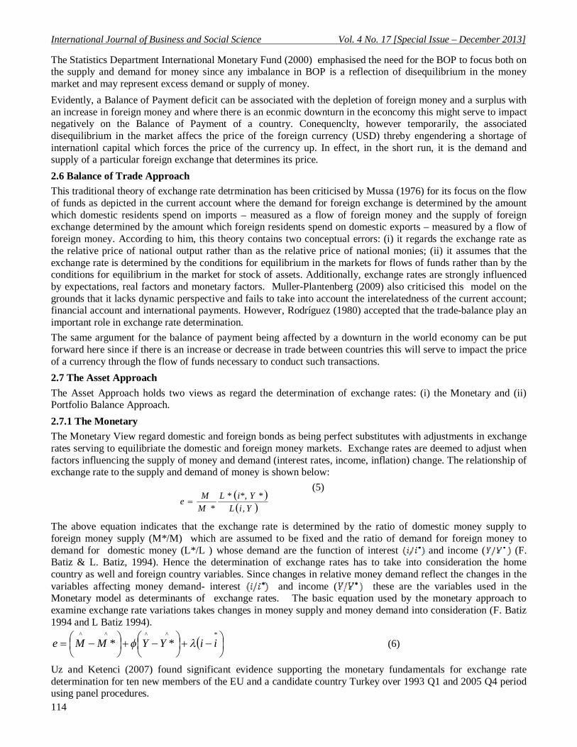
The Monetary View regard domestic and foreign bonds as being perfect substitutes with adjustments in exchange rates serving to equilibriate the domestic and foreign money markets. Exchange rates are deemed to adjust when factors influencing the supply of money and demand (interest rates, income, inflation) change. The relationship of exchange rate to the supply and demand of money is shown below:

(5)

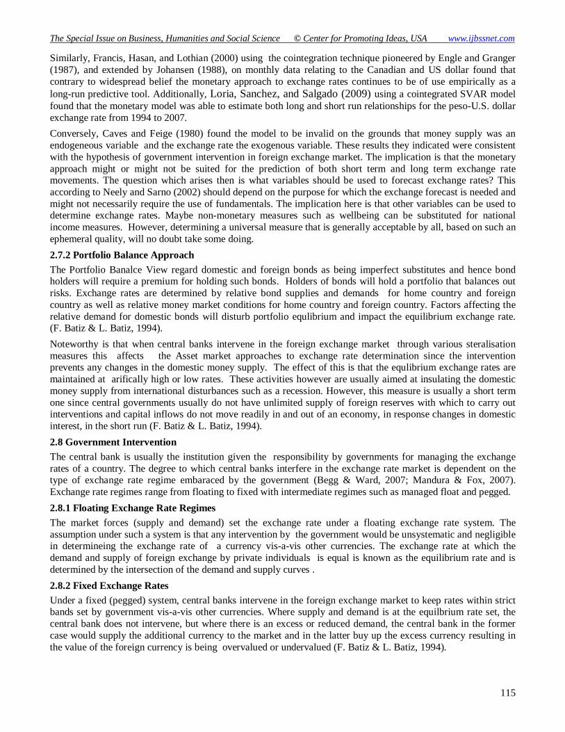
The above equation indicates that the exchange rate is determined by the ratio of domestic money supply to foreign money supply (M*/M) which are assumed to be fixed and the ratio of demand for foreign money to demand for domestic money (L*/L ) whose demand are the function of interest and income ( (F. Batiz & L. Batiz, 1994). Hence the determination of exchange rates has to take into consideration the home country as well and foreign country variables. Since changes in relative money demand reflect the changes in the variables affecting money demand- interest and income ( these are the variables used in the Monetary model as determinants of exchange rates. The basic equation used by the monetary approach to examine exchange rate variations takes changes in money supply and money demand into consideration (F. Batiz 1994 and L Batiz 1994).

*^^^^** iiYYMMe (6)

Uz and Ketenci (2007) found significant evidence supporting the monetary fundamentals for exchange rate determination for ten new members of the EU and a candidate country Turkey over 1993 Q1 and 2005 Q4 period using panel procedures.

YiL

YiLMMe

,**,*

*


115

Similarly, Francis, Hasan, and Lothian (2000) using the cointegration technique pioneered by Engle and Granger (1987), and extended by Johansen (1988), on monthly data relating to the Canadian and US dollar found that contrary to widespread belief the monetary approach to exchange rates continues to be of use empirically as a long-run predictive tool. Additionally, Loria, Sanchez, and Salgado (2009) using a cointegrated SVAR model found that the monetary model was able to estimate both long and short run relationships for the peso-U.S. dollar exchange rate from 1994 to 2007.

Conversely, Caves and Feige (1980) found the model to be invalid on the grounds that money supply was an endogeneous variable and the exchange rate the exogenous variable. These results they indicated were consistent with the hypothesis of government intervention in foreign exchange market. The implication is that the monetary approach might or might not be suited for the prediction of both short term and long term exchange rate movements. The question which arises then is what variables should be used to forecast exchange rates? This according to Neely and Sarno (2002) should depend on the purpose for which the exchange forecast is needed and might not necessarily require the use of fundamentals. The implication here is that other variables can be used to determine exchange rates. Maybe non-monetary measures such as wellbeing can be substituted for national income measures. However, determining a universal measure that is generally acceptable by all, based on such an ephemeral quality, will no doubt take some doing.

2.7.2 Portfolio Balance Approach

The Portfolio Banalce View regard domestic and foreign bonds as being imperfect substitutes and hence bond holders will require a premium for holding such bonds. Holders of bonds will hold a portfolio that balances out risks. Exchange rates are determined by relative bond supplies and demands for home country and foreign country as well as relative money market conditions for home country and foreign country. Factors affecting the relative demand for domestic bonds will disturb portfolio equlibrium and impact the equilibrium exchange rate. (F. Batiz & L. Batiz, 1994).

Noteworthy is that when central banks intervene in the foreign exchange market through various steralisation measures this affects the Asset market approaches to exchange rate determination since the intervention prevents any changes in the domestic money supply. The effect of this is that the equlibrium exchange rates are maintained at arifically high or low rates. These activities however are usually aimed at insulating the domestic money supply from international disturbances such as a recession. However, this measure is usually a short term one since central governments usually do not have unlimited supply of foreign reserves with which to carry out interventions and capital inflows do not move readily in and out of an economy, in response changes in domestic interest, in the short run (F. Batiz & L. Batiz, 1994).

2.8 Government Intervention

The central bank is usually the institution given the responsibility by governments for managing the exchange rates of a country. The degree to which central banks interfere in the exchange rate market is dependent on the type of exchange rate regime embaraced by the government (Begg & Ward, 2007; Mandura & Fox, 2007). Exchange rate regimes range from floating to fixed with intermediate regimes such as managed float and pegged.

2.8.1 Floating Exchange Rate Regimes

The market forces (supply and demand) set the exchange rate under a floating exchange rate system. The assumption under such a system is that any intervention by the government would be unsystematic and negligible in determineing the exchange rate of a currency vis-a-vis other currencies. The exchange rate at which the demand and supply of foreign exchange by private individuals is equal is known as the equilibrium rate and is determined by the intersection of the demand and supply curves .

2.8.2 Fixed Exchange Rates

Under a fixed (pegged) system, central banks intervene in the foreign exchange market to keep rates within strict bands set by government vis-a-vis other currencies. Where supply and demand is at the equilbrium rate set, the central bank does not intervene, but where there is an excess or reduced demand, the central bank in the former case would supply the additional currency to the market and in the latter buy up the excess currency resulting in the value of the foreign currency is being overvalued or undervalued (F. Batiz & L. Batiz, 1994).


116

2.8.3 Managed Floating

Under a managed floating system the central bank uses its judgement with respect to the degree of interferrence in the foreign exhange market. They usually do not have specified targets at which to aim. Indicators such as balance of payments position, international rserves, parallel markets developments usually trigger such responses which may be direct or indirect (International Monetary Fund, 2006).

2.9 The Market Microstructure Approach

The difficulties associated with the detemination of exchange rates in the short run using traditional models has lead to the development of the Market Microstructure Approach to Exchange Rate Determination. This approach seeks to overcome the inability of traditional models to control for macro news effects on exchange rate dynamics and to carry out any meaningful analysis of exchange rate determination in the short run(Vitale, 2007).

The Market Microstructure Approach Approach to Exchange Rate Determiantion views exchange rates as being determined by the interaction among investors at a micro level. These investors minimise their risk by constantly adjusting their price (bid/ask) throughout the day in order to balance their portfolios so that at the end of the day the market clears. These investors also adjust their quotes (bid/ask) in the belief that the person placing an order is in possession of information about current market conditions that the trader does not know or in response to government activities in the foreign exchange market. When government intervene in this way it signals changes in government’s monetary policy and hence affect market expectations regarding the fundamentals and utlimately impact the price of a currency (Vitale, 2007). This clearly contracdicts the other approaches to exchange rate determination and implies that traders/investors reaction to order flows and news effect changes in the exchange rate and not supply and demand through the fundamentals. However, according to Vitale (2007) more work is needed before it can be argued that the market microstructure approach is the solution to valid exchange rate forecasts.

The conclusion can be drawn that this model is far from perfect. Evidently, the argument that at the end of the day the market clears needs to be examined and raises some questions. What happens if traders/investors do not behave in this way? What happens if, when there is news of a change in economic conditions whether in the domestic country or globally, that instead of clearing the market these traders/investors manipulate the price of the currecny by storing it thereby artifically creating a shortage and then collude and set the prices at a later date rather than allow the market to determine the equilibrium rate? Clearly, these are some issues which this model needs to address if it is to be regarded as the solution for valid exchange rate forecasts.

3. Methodology

3.1 Introduction

The objective of the investigation was to determine the impact of the recession in the United States on the spot (selling/ask) price of the United States Dollar in Guyana. To this end two questions were asked: (i) How has the demand for USD affected its spot ask/selling price since the recession in the United States? (ii) How has the supply of USD affected its spot ask/selling price since the recession in the United States? Consequently, it was hypothesised that:

OH There is no relationship between the spot (ask) selling price of the US$ and supply since the recession

0H There is no relationship between the spot (ask) selling price of the US$ and demand since the recession

1H There is a relationship between the spot (ask) selling price of the US$ and supply since the recession

1H There is a relationship between the spot (ask) selling price of the US$ and demand since the recession

The following outlines the methodology used to derive answers to the questions:

3.2 Data Collection

Archival content analysis of online data bases for the Bank of Guyana; US Census Bureau, and the Federal Reserve Statistics was employed to gather the data for the study which comprised the spot exchange rate of the USD, interest rate, money supply and income for the period January 2006 to December 2008. This provided data points for three years. In total the data set consisted quarterly observations each for the four variables (spot price, money supply, income, and interest) for the pre-crisis period and seven quarterly observations each for the four variables (spot price, money supply, income and interest) for the crisis period.


117

3.3 Procedure

Since one of the variables collected for the analysis was tabulated as quarterly data the monthly data collected was similarly transformed. Additionally, the data measured in US currency was translated to Guyanese dollars using the quarterly average exchange rate for the periods under investigation. The effect of the impact of the recession in the United States on the Spot/ask price of USD in Guyana, through its supply and demand, was investigated by dividing the data (variables relating to the spot price of USD and fundamentals) into two sub periods. The pre-crisis behaviour is analysed on the first sub-sample ranging from January 2006 to April 2007 providing 5 observations relating to the dependent variable spot price and the independent variables the ratios of money supply, income and interest. The crisis behaviour was captured through the second sample running from May 2007 to December 2008, with 7 observations each relating to the dependent variable spot price and the independent variables the ratios of money supply, income, and interest.

3.4 Research Model

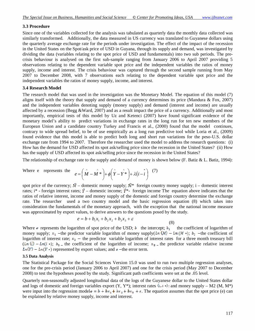
The research model that was used in the investigation was the Monetary Model. The equation of this model (7) aligns itself with the theory that supply and demand of a currency determines its price (Mandura & Fox, 2007) and the independent variables denoting supply (money supply) and demand (interest and income) are usually affected by a recession (Begg &Ward, 2007) and as a result impact the price of a currency. Additionally and most importantly, empirical tests of this model by Uz and Ketenci (2007) have found significant evidence of the monetary model’s ability to predict variations in exchange rates in the long run for ten new members of the European Union and a candidate country Turkey and Francis et al., (2000) found that the model continues, contrary to wide spread belief, to be of use empirically as a long run predictive tool while Loria et al., (2009) found evidence that this model is able to predict both long and short run variations for the peso-U.S. dollar exchange rate from 1994 to 2007. Therefore the researcher used the model to address the research questions: (i) How has the demand for USD affected its spot ask/selling price since the recession in the United States? (ii) How has the supply of USD affected its spot ask/selling price since the recession in the United States?

The relationship of exchange rate to the supply and demand of money is shown below (F. Batiz & L. Batiz, 1994): Where e represents the (7) spot price of the currency; – domestic money supply; * foreign country money supply; i – domestic interest rates; i* - foreign interest rates; – domestic income; *- foreign income The equation above indicates that the ratios of relative interest, income and money supply of the domestic and foreign country determine the exchange rate. The researcher used a two country model and the basic regression equation (8) which takes into consideration the fundamentals of the monetary approach, with the exception that the national income measure was approximated by export values, to derive answers to the questions posed by the study. (8) Where represents the logarithm of spot price of the USD; the intercept; the coefficient of logarithm of money supply; the predictor variable logarithm of money supply( ; the coefficient of logarithm of interest rate; the predictor variable logarithm of interest rates for a three month treasury bill ( ; the coefficient of the logarithm of income; the predictor variable relative income

represented by export values; and the error term.

3.5 Data Analysis

The Statistical Package for the Social Sciences Version 15.0 was used to run two multiple regression analyses, one for the pre-crisis period (January 2006 to April 2007) and one for the crisis period (May 2007 to December 2008) to test the hypotheses posed by the study. Significant path coefficients were set at the .05 level.

Quarterly non-seasonally adjusted longitudinal data of the logs of the Guyanese dollar to the United States dollar and logs of domestic and foreign variables export (Y, Y*); interest rates and money supply – M2 (M, M*) were input into the regression model . The equation assumes that the spot price (e) can be explained by relative money supply, income and interest.

*^^^^** iiYYMMe

332211 xbxbxbbe

*^^^^** iiYYMMe


118

This equation also assumes that the explanatory variables of supply (money supply) and demand (interest and income) are non-stochastic and independent of the error term.

It is this assumption that allows the model to be estimated using Ordinary Least Square (OLS). Additionally, other researchers, for example, Husted and McDonald (1999) successfully used this method (based on panel estimates) to analyse the contributions of the fundamentals of the monetary model to the Asian crisis. However, OLS analysis has been criticised by Binkley (1980) on the grounds that justifying its use based on the elasticity nature of supply by some researchers is not a sufficient criteria for accepting small bias in least squares estimation since such a causal relationship is at best a spurious one. The researcher is aware that there are other tests such as co-integration used by Francis et al., (2000) that are regarded as being quite robust in their application with regard to the determination of exchange rates. However, the aim of the research was not to forecast future spot exchange rates but to identify whether or not supply and demand influenced movements in the spot exchange rates during the periods under investigation.

3.6 Validity of research using OLS

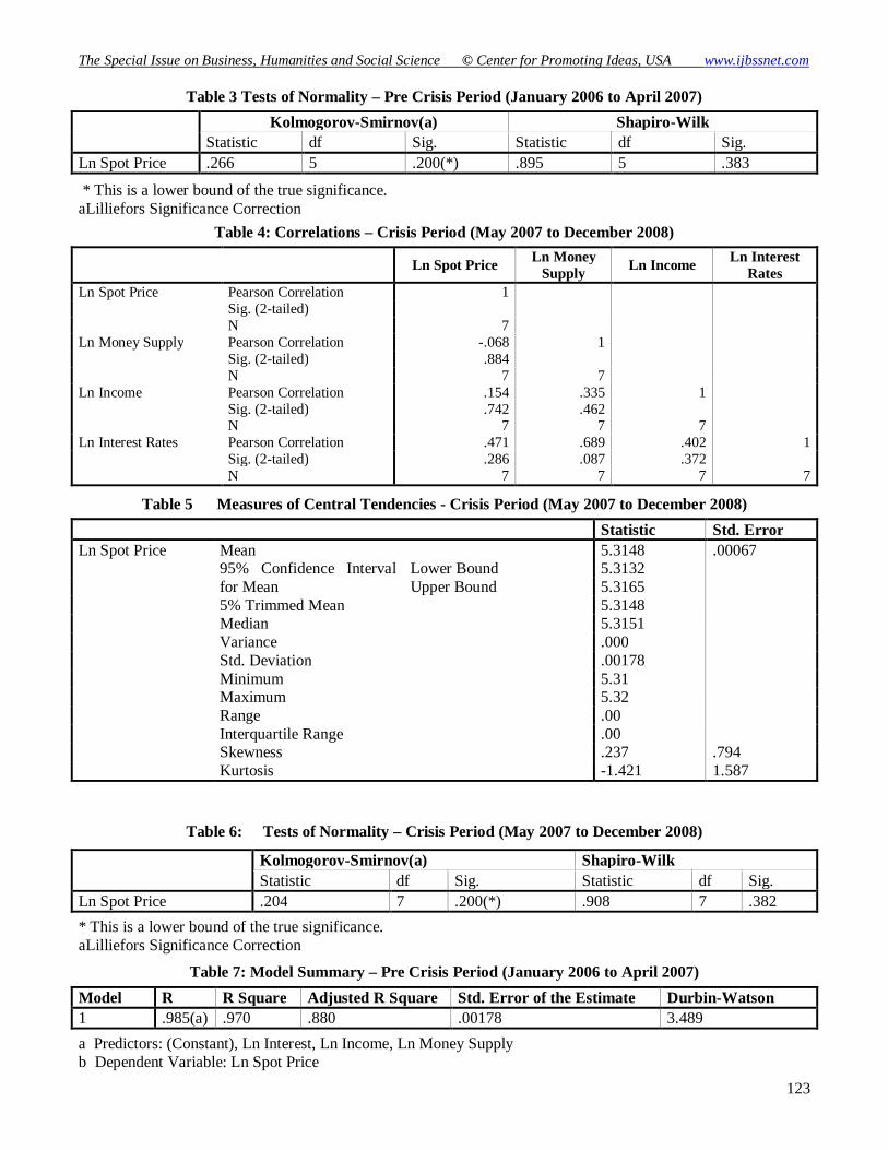
To assure the validity of research, the researcher has to ensure that good research procedures; adequate samples and accurate measurements are used (Collis & Hussey, 2009). The validity of research results are usually enhanced when the priori assumptions of the particular test to be used are met. Consequently, prior to statistically analyzing the data the assumptions of linear regression analysis were ascertained through checks for collinearity, linearity and normality. The statistics revealed that there were no significant departures from normality, the absence of collinearity among the independent variables and that the variables were linearly related for the pre-crisis and crisis period (Tables 1, 2, 3, 4, 5, 6).

4. Results

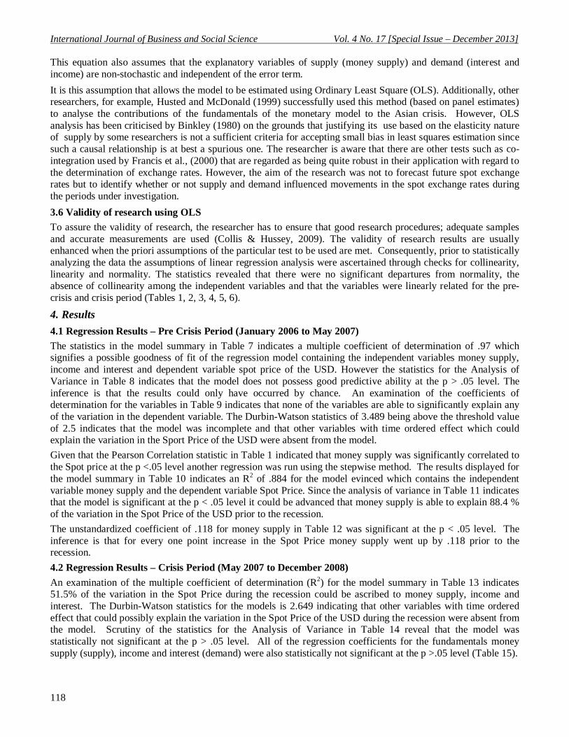
4.1 Regression Results – Pre Crisis Period (January 2006 to May 2007)

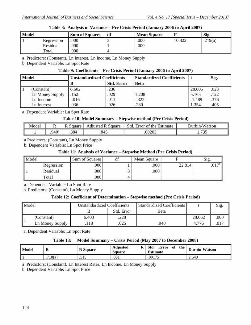
The statistics in the model summary in Table 7 indicates a multiple coefficient of determination of .97 which signifies a possible goodness of fit of the regression model containing the independent variables money supply, income and interest and dependent variable spot price of the USD. However the statistics for the Analysis of Variance in Table 8 indicates that the model does not possess good predictive ability at the p > .05 level. The inference is that the results could only have occurred by chance. An examination of the coefficients of determination for the variables in Table 9 indicates that none of the variables are able to significantly explain any of the variation in the dependent variable. The Durbin-Watson statistics of 3.489 being above the threshold value of 2.5 indicates that the model was incomplete and that other variables with time ordered effect which could explain the variation in the Sport Price of the USD were absent from the model.

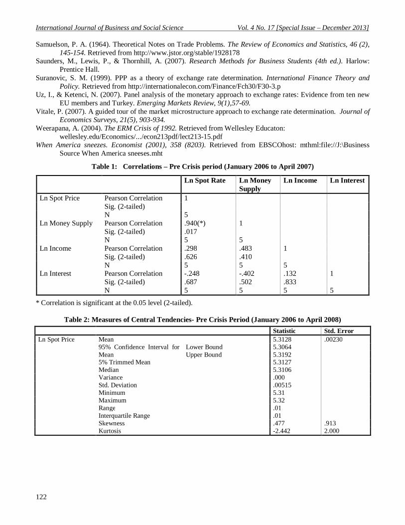
Given that the Pearson Correlation statistic in Table 1 indicated that money supply was significantly correlated to the Spot price at the p <.05 level another regression was run using the stepwise method. The results displayed for the model summary in Table 10 indicates an R2 of .884 for the model evinced which contains the independent variable money supply and the dependent variable Spot Price. Since the analysis of variance in Table 11 indicates that the model is significant at the p < .05 level it could be advanced that money supply is able to explain 88.4 % of the variation in the Spot Price of the USD prior to the recession.

The unstandardized coefficient of .118 for money supply in Table 12 was significant at the p < .05 level. The inference is that for every one point increase in the Spot Price money supply went up by .118 prior to the recession.

4.2 Regression Results – Crisis Period (May 2007 to December 2008)

An examination of the multiple coefficient of determination (R2) for the model summary in Table 13 indicates 51.5% of the variation in the Spot Price during the recession could be ascribed to money supply, income and interest. The Durbin-Watson statistics for the models is 2.649 indicating that other variables with time ordered effect that could possibly explain the variation in the Spot Price of the USD during the recession were absent from the model. Scrutiny of the statistics for the Analysis of Variance in Table 14 reveal that the model was statistically not significant at the p > .05 level. All of the regression coefficients for the fundamentals money supply (supply), income and interest (demand) were also statistically not significant at the p >.05 level (Table 15).


119

Consequently the null the hypotheses are accepted that: (i) 0H There is no relationship between the spot (ask) selling price of the US$ and supply since the recession and (ii) 0H There is no relationship between the spot (ask) selling price of the US$ and demand since the recession

5. Discussion

5.1 The pre-crisis period

According to the monetary model the fundamentals of money supply, income and interest influence the variability in the price of a currency (F. Batiz & L. Batiz, 1994). Multiple regression analysis conducted on the data prior to the recession – pre-crisis period which ranged from January 2006 to April 2007 indicated that the model was a good fit but statistically insignificant (Table 7). However the results of the stepwise method revealed that the model that best fitted the data was a bivariate one between money supply and the spot exchange rate. The model indicated that only supply as denoted by the independent variable money supply was statistically significant at the p <.05 level in explaining 88.4 % of the variation in the spot price of the USD in Guyana during pre-crisis period. The sign of the coefficient of supply (money supply) was positive indicating that an increase in supply (money supply) placed a downward pressure (depreciation) on the Guyanese Dollar during this period.

This is consistent with a floating exchange rate regime where market forces set the equilibrium price of a currency and implies a lack of intervention in the foreign exchange market by the government (F. Batiz & L. Batiz, 1994) which in a period of calm would not have necessitated any intervention by central banks. The positive regression coefficient of supply (money supply) and an R2 88.4 % lends support to the monetary view that money supply influences the exchange rate of a currency. The ability of the other independent (demand) variables income and interest to influence the spot price could not be statistically confirmed and is inconsistent with the view of Francis et al., (2000); Loria et al., (2009); Uz and Ketenci (2007) that the monetary approach to exchange rates continues to be of use empirically as either a long run or as determined by Loria et al., (2009), a short run predictive tool of exchange rate determination. This may be indicative of the monetary fundamentals not being sole influencers of the price of the USD during the pre-crisis period and that other explanatory variables, with time ordered effect on the dependent variable spot price, were absent from the model. However, the Durbin Watson statistics of 1.735 being less than the rule of thumb 2.5 does not support this analysis.

5.2 The crisis period

In comparison, the statistics of the crisis period which ranged from May 2007 to December 2008 indicated that 51.5 % in the variation in the spot price of the USD was solely the result of demand (interest) and supply (money supply) and that the income component of demand did not account for any of the variation in the spot price of the USD. In fact its coefficient was 0.000 indicating the 1% increase in income did not account for any of the variability in the spot price of the USD during this period. The statistics were however, not significant at the 5% level. The indication of the coefficient of 0.000 for income, as measured by export values, is not entirely surprising since contractual arrangements may have existed which served to lock in export trade in terms of quantity and price and hence the recession did not impact these terms of trade in the short run. Another possible explanation could be that even though there was a decline in production and unemployment was on the rise globally, that this did not influence the demand for Guyanese products hence money demand as measured by income (export values) would have been left relatively unchanged with no impact on the spot price of the USD.

The F test results which are known to be quite robust with regard to departures from non-normality indicated that the monetary model was inadequate as an analytical and predictive tool in explaining exchange rate variations during the period.

Consequently, no statistically significant conclusions can be drawn that either supply and/or demand for the USD influenced the spot price of the USD during the recession (crisis period). As a result, the findings of Pollard (2000) that the US money supply is a major source of international disturbance for Guyana is not supported.

High employment is usually a primary goal of economic policy and when in conflict as a result of some disturbance, for example a recession, governments intervene in the foreign exchange market in response to this goal thereby preventing a balance of payment adjustment from occurring through a recession. Such interventions usually take the form of either direct or indirect sterilisation measures and leave the money supply unchanged.


120

Consequently, this action may have served to prevent the market forces of demand and supply from equilibrating the exchange rate of the USD (F. Batiz & L. Batiz, 1994). Implied here is that the exchange rate regime of the government is either fixed or controlled floating.

Noteworthy is the Durbin Watson statistics of 2.649 for the model which indicates that that the multivariate model, evidenced through the backward selection process, was incomplete at the p <.05 and that other independent variables, that had time ordered effect on the dependent variable, spot price of the USD, were absent from the model. Since, government intervention was not catered for in the model this a possible reason for the lack of significance in the results regarding money supply being an influencer of the price of the USD. Such interventions might have interfered with the workings of the foreign exchange market mechanisms and therefore demand and supply of the USD would not have equilibrated the spot price of the USD during this period.

Additionally, the results are inconsistent with those of Francis et al., (2000); Loria et al., (2009); Uz and Ketenci (2007) that the monetary approach to exchange rates continues to be of use empirically as either a long run or Loria et al., (2009) a short run predictive tool of exchange rate determination but consistent with the results of Caves and Feige (1980) that the monetary model was invalid because money supply was an endogenous (dependent) variable while the exchange rate was the exogeneous (independent) variable which is consistent with the hypothesis of government intervention in the exchange market. This casts doubts, yet again, on the adequacy of the monetary model to predict exchange rate variation and the fundamentals being sole influencers of exchange rates. Moreover, the results imply that other variables maybe those proposed by other approaches to exchange rate determination such as the Market Microstructure approach; the Balance of Payment approach; the Balance of Trade approach; Portfolio Balance approach might have influenced the spot exchange rate during the crisis period under review. The results are however consistent with the view of Neely and Sarno (2002) that foreign exchange forecasts may not necessarily require the use of fundamentals and that the purpose for which the forecast is needed should dictate the variables to be used. The implications are that other variables beside those identified by the monetary approach could be used to determine exchange rate variation bearing in mind the purpose of the study.

6. Conclusion

Evidently, supply (money supply) and demand (interest, export values - a component of national income measures used as an approximation of the independent variable income in the study) did not have a statistically significant impact on the spot price of the USD during the crisis period. Hence the null hypotheses were accepted that (i) there is no relationship between the spot (ask) selling price of the US$ and supply since the recession at the p > .05 level and (ii) there is no relationship between the spot (ask) selling price of the US$ and demand since the recession at the p > .05 level. The conclusion is therefore drawn that supply and demand did not influence the spot price of the USD in Guyana during the crisis period under investigation. And, to answer the question initially posed, Guyana did not catch a cold when America sneezed.

6.1 Limitations of research and directions for future research

The small sample sizes, short sampling time period, and inability to access national income measures in the required format influenced the results. The presence of autocorrelation in the data indicating the absence of other independent variables from the model also impacted the results. The study can be further refined by extending the period of investigation since the effects of the recession may indeed have been a slow ‘spill over’ one as described by (Kaminsky et al., 2003).

Additionally, the use of more robust test such as conintegration techniques and incorporating other independent variables in the model may help to better analyse the effects of the recession on the spot price of the USD in Guyana.


121

References

Ackermann, J. (2008). The subprime crisis and its consequences. Journal of Financial Stability 4, 329–337. Arsham, H. (n.d.). Time Series Analysis For Business Forecasting. Retrieved from

http://home.ubalt.edu/ntsbarsh/stat-data/Forecats.htm Balassa, B. (1964). The Purchasing-Power Parity Doctrine: A Reappraisal. The Jounal of Political Economics, 72

(6), 584-596 Batiz, F. R., & Batiz, L. A. (1994). International finance and open economy macroeconomics.(2nd. ed.). New

Jersey: Prentice Hall. Begg, D., & Ward, D. (2007). Economics for business (2nd ed.). London: Mc Graw Hill. Binkley, J. K. (1980). The relationship between elasticity and least squares. The Review of Economics and

Statistics 63(2), 307-309. Retrieved from http://www.jstor.org/stable/1924104 Caves, D. W., & Feige, E. L. (1980). Efficient Foreign Exchange Markets and the Monetary Approach to

Exchange-Rate Determination. The American Economic Review,70(1), 120-134. Retrieved from http://www.jstor.org/stable/1814742 Collis, J., & Hussey, R. (2009). Business research a practical guide for undergraduate & post graduate students.

(3rd ed.). Palgrage Macmillan. Dornbusch, R., & Krugman, P. (1976). Flexible exchange rates in the short run. Brookings Papers on Economic

Activity, 3, 537-584. Retrieved from http://www.jstor.org/stable/2534369 Francis, B., Hasan, I., & Lothian, J. R. (2000). The Monetary Approach to Exchange Rates and the Canadian

Dollar over the Long Run. The Applied Financial Economics. Retrieved from http://ssrn.com/abstract=613908

Fund, I. M. (2006). De Facto Classifications of Exchange Rate Regimes and Monetary Policy Framework. Retrieved: http://www.imf.org/external/np/mfd/er/2006

Groebner, D. F., Shannon, P. W., Fry, P. C., & Smith, K. D. (2005). Business statistics a decision-making approach. (6th ed.). New Jersey: Prentice Hall.

Husted, S., & McDonald, R. (1999). The Asian currency crash: were badly driven fundamentals to blame?Journal of Asian Economics, 10(4), 537-550.

Kaminsky, G. L., Reinhart, C. M., & Vegh, C. A. (2003). Unholy Trinity of Financial Contagion. Journal of Economic Perspectives. 17(4), 51-74. Retrieved from http://www.jstor.org/stable/3216931.

Keller, G. (2001). Applied Statistics with Microsoft Excell. Australia: THOMSON LEARNING. Lipsey, R. G., & Chrystal, K. A. (1999). Principles of Economics (9th. ed.). Oxford: Oxford University Press. Loria, E., Sanchez, A., & Salgado, U. (2009). New Evidence on the monetray approach of exchange rate

determination in Mexico 1994-2007: A cointegrated SVAR model. Journal of International Money and Finance, 29(3), 540-554. doi:10.1016/j.jimonfin.2009.07.007

Lucey, T. (2000). Quantative Techniques (5th ed.). London: Letts Educational. Mandura, J., & Fox, R. (2007). International Financial Management. . Australia: Thompson. Melicher, R. W., & Welshand, M. T. (1992). Finance Introduction to Markets Institutions & Management, (8th

ed.). Cincinnati Ohio: South Western Pulishing. Muller-Plantenberg, N. A. (2009). Balance of payments accounting and exchange rate dynamics. Journal of

International Review of Economics and Finance, 19(1), 46-63. Mussa, M. (1976). The exchange rate, the balance of payments and monetary and fiscal policy under a regime of

controlled floating.The Scandinavian Journal of Economics, 78(2), 229-248. Retrieved from http://www.jstor.org/stable/3439926 Neely, C. J., & Sarno, L. (2002). How Well Do Monetary Models Forecast Exchange Rates? Federal Reserve

Bank of St. Louis Review, 84(5), 51-74. Pollard, S. K. (2000). Foreign exchange market pressure and transmission of international disturbances: the case

of Barbados, Guyana, Jamaica, and Trinidat & Tobago. Retrieved from Applied Economics Letters: http://www.informaworld.com/smpp/content

Reuters. (2008). Credit crunch will hurt developing countries, World Bank says. Retrieved from International Herals: mthml:file://G:\Credit crunch will hurt developing countries, World Bank says

Rodríguez, C. A. (1980). The Role of Trade Flows in Exchange Rate Determination: A Rational Expectations Approach. The Journal of Political Economy, 88(6), 1148-1158. Retrieved from http://www.jstor.org/stable/1831159


122

Samuelson, P. A. (1964). Theoretical Notes on Trade Problems. The Review of Economics and Statistics, 46 (2),

145-154. Retrieved from http://www.jstor.org/stable/1928178 Saunders, M., Lewis, P., & Thornhill, A. (2007). Research Methods for Business Students (4th ed.). Harlow:

Prentice Hall. Suranovic, S. M. (1999). PPP as a theory of exchange rate determination. International Finance Theory and

Policy. Retrieved from http://internationalecon.com/Finance/Fch30/F30-3.p Uz, I., & Ketenci, N. (2007). Panel analysis of the monetary approach to exchange rates: Evidence from ten new

EU members and Turkey. Emerging Markets Review, 9(1),57-69. Vitale, P. (2007). A guided tour of the market microstructure approach to exchange rate determination. Journal of

Economics Surveys, 21(5), 903-934. Weerapana, A. (2004). The ERM Crisis of 1992. Retrieved from Wellesley Educaton:

wellesley.edu/Economics/.../econ213pdf/lect213-15.pdf When America sneezes. Economist (2001), 358 (8203). Retrieved from EBSCOhost: mthml:file://J:\Business

Source When America sneeses.mht

Table 1: Correlations – Pre Crisis period (January 2006 to April 2007)

Ln Spot Rate Ln Money Supply

Ln Income Ln Interest

Ln Spot Price Pearson Correlation 1 Sig. (2-tailed) N 5

Ln Money Supply Pearson Correlation .940(*) 1 Sig. (2-tailed) .017 N 5 5

Ln Income Pearson Correlation .298 .483 1 Sig. (2-tailed) .626 .410 N 5 5 5

Ln Interest Pearson Correlation -.248 -.402 .132 1 Sig. (2-tailed) .687 .502 .833 N 5 5 5 5

* Correlation is significant at the 0.05 level (2-tailed).

Table 2: Measures of Central Tendencies- Pre Crisis Period (January 2006 to April 2008)

Statistic Std. Error Ln Spot Price Mean 5.3128 .00230

95% Confidence Interval for Mean

Lower Bound 5.3064 Upper Bound 5.3192

5% Trimmed Mean 5.3127 Median 5.3106 Variance .000 Std. Deviation .00515 Minimum 5.31 Maximum 5.32 Range .01 Interquartile Range .01 Skewness .477 .913 Kurtosis -2.442 2.000


123

Table 3 Tests of Normality – Pre Crisis Period (January 2006 to April 2007)

Kolmogorov-Smirnov(a) Shapiro-Wilk

Statistic df Sig. Statistic df Sig. Ln Spot Price .266 5 .200(*) .895 5 .383

* This is a lower bound of the true significance. aLilliefors Significance Correction

Table 4: Correlations – Crisis Period (May 2007 to December 2008)

Ln Spot Price Ln Money Supply Ln Income Ln Interest

Rates Ln Spot Price Pearson Correlation 1

Sig. (2-tailed) N 7

Ln Money Supply Pearson Correlation -.068 1 Sig. (2-tailed) .884 N 7 7

Ln Income Pearson Correlation .154 .335 1 Sig. (2-tailed) .742 .462 N 7 7 7

Ln Interest Rates Pearson Correlation .471 .689 .402 1 Sig. (2-tailed) .286 .087 .372 N 7 7 7 7

Table 5 Measures of Central Tendencies - Crisis Period (May 2007 to December 2008)

Statistic Std. Error Ln Spot Price Mean 5.3148 .00067

95% Confidence Interval for Mean

Lower Bound 5.3132 Upper Bound 5.3165

5% Trimmed Mean 5.3148 Median 5.3151 Variance .000 Std. Deviation .00178 Minimum 5.31 Maximum 5.32 Range .00 Interquartile Range .00 Skewness .237 .794 Kurtosis -1.421 1.587

Table 6: Tests of Normality – Crisis Period (May 2007 to December 2008)

Kolmogorov-Smirnov(a) Shapiro-Wilk Statistic df Sig. Statistic df Sig.

Ln Spot Price .204 7 .200(*) .908 7 .382

* This is a lower bound of the true significance. aLilliefors Significance Correction

Table 7: Model Summary – Pre Crisis Period (January 2006 to April 2007)

Model R R Square Adjusted R Square Std. Error of the Estimate Durbin-Watson 1 .985(a) .970 .880 .00178 3.489

a Predictors: (Constant), Ln Interest, Ln Income, Ln Money Supply b Dependent Variable: Ln Spot Price


124

Table 8: Analysis of Variance – Pre Crisis Period (January 2006 to April 2007)

Model Sum of Squares df Mean Square F Sig. 1 Regression .000 3 .000 10.822 .219(a)

Residual .000 1 .000 Total .000 4

a Predictors: (Constant), Ln Interest, Ln Income, Ln Money Supply b Dependent Variable: Ln Spot Rate

Table 9: Coefficients – Pre Crisis Period (January 2006 to April 2007)

Model Unstandardized Coefficients Standardized Coefficients t Sig. B Std. Error Beta 1 (Constant) 6.602 .236 28.005 .023 Ln Money Supply .152 .029 1.208 5.165 .122 Ln Income -.016 .011 -.322 -1.489 .376 Ln Interest .036 .026 .280 1.354 .405

a Dependent Variable: Ln Spot Rate

Table 10: Model Summary – Stepwise method (Pre Crisis Period)

Model R R Square Adjusted R Square Std. Error of the Estimate Durbin-Watson 1 .940a .884 .845 .00203 1.735

a Predictors: (Constant), Ln Money Supply b. Dependent Variable: Ln Spot Price

Table 11: Analysis of Variance – Stepwise Method (Pre Crisis Period)

Model Sum of Squares df Mean Square F Sig.

1 Regression .000 1 .000 22.814 .017b Residual .000 3 .000 Total .000 4

a. Dependent Variable: Ln Spot Rate b. Predictors: (Constant), Ln Money Supply

Table 12: Coefficient of Determination – Stepwise method (Pre Crisis Period)

Model Unstandardized Coefficients Standardized Coefficients t Sig. B Std. Error Beta

1 (Constant) 6.403 .228 28.062 .000 Ln Money Supply .118 .025 .940 4.776 .017

a. Dependent Variable: Ln Spot Rate

Table 13: Model Summary – Crisis Period (May 2007 to December 2008)

Model R R Square Adjusted R Square

Std. Error of the Estimate Durbin-Watson

1 .718(a) .515 .031 .00175 2.649

a Predictors: (Constant), Ln Interest Rates, Ln Income, Ln Money Supply b Dependent Variable: Ln Spot Price


125

Table 14: Analysis of Variance – Crisis Period (May 2007 to December 2008)

Model Sum of Squares df Mean Square F Sig. 1 Regression .000 3 .000 1.063 .481(a)

Residual .000 3 .000 Total .000 6

a Predictors: (Constant), Ln Interest Rates, Ln Income, Ln Money Supply b Dependent Variable: Ln Spot Price

Table 15: Coefficients – Crisis Period (May 2007 to December 2008)

Model

Unstandardized Coefficients Standardized Coefficients t Sig. B Std. Error Beta

1 (Constant) 5.016 .226 22.172 .000 Ln Money Supply -.033 .024 -.749 -1.345 .271 Ln Income .000 .008 .010 .023 .983 Ln Interest Rates .002 .001 .983 1.715 .185

a Dependent Variable: Ln Spot Price

the impact of the recession in the united states on the...

Documents