the impact of general non-parametric volatility functions in multivariate garch models
TRANSCRIPT
Computational Statistics & Data Analysis 50 (2006) 3032–3052www.elsevier.com/locate/csda
The impact of general non-parametric volatilityfunctions in multivariate GARCH models�
Francesco Audrino∗Institute of Finance, University of Lugano, Via Buffi 13, 6900 Lugano, Switzerland
Received 6 June 2005; received in revised form 6 June 2005; accepted 6 June 2005Available online 11 July 2005
Abstract
Recent studies have revealed that financial volatilities and correlations move together over timeacross assets and markets. The main effort has been on improving the flexibility of conditional corre-lation dynamics, while maintaining computational feasibility for large estimation problems. However,since in such models conditional covariances are the product of conditional correlations and individualvolatilities, it is plausible that improving the estimation of individual volatilities will lead to bettercovariance forecasts, too. Functional gradient descent (FGD) has already been shown to improve sub-stantially in-sample and out-of-sample covariance accuracy in the very simple constant conditionalcorrelation (CCC) setting. Following this direction, the impact of FGD volatility estimates is testedin several multivariate GARCH settings, both at the multivariate and at the univariate portfolio levels.In particular, improving conditional correlations and improving individual volatilities are compared,to establish which effect produces the best fits and predictions for conditional covariances.© 2005 Elsevier B.V. All rights reserved.
Keywords: Multivariate GARCH models; Asymmetric non-linear volatility; Dynamic conditional correlations;Functional gradient descent (FGD) estimation
1. Introduction
The volatility matrix is a basic ingredient in financial econometrics, owing to its centralrole in many practical applications as, for example, those related to risk management.
� Funded by a grant from the Foundation of Research and Development of the University of Lugano.∗ Tel.: +41586664789; fax: +41586664647.
E-mail address: [email protected].
0167-9473/$ - see front matter © 2005 Elsevier B.V. All rights reserved.doi:10.1016/j.csda.2005.06.006

F. Audrino / Computational Statistics & Data Analysis 50 (2006) 3032–3052 3033
Nowadays, there is clear empirical evidence that both financial volatilities and correlationsmove together over time across assets and markets. For this reason, recent studies havefocused on the building of dynamic multivariate models to estimate and forecast trulyconditional covariance matrices. However, this could be an incredibly difficult task becauseof the curse of dimensionality and additional model selection problems when the dimensionincreases. In particular, when the number of individual positions or assets is extremely large,the models must remain computationally feasible by keeping a reasonable complexity inthe dynamics.
A large class of widely accepted models for estimating financial conditional covari-ance matrices is that consisting of multivariate GARCH-type models. Of particular interestare multivariate GARCH models, which estimate individual volatilities and conditionalcorrelations separately, using a two-stage estimation procedure, and then compute condi-tional covariances as products of individual volatilities and conditional correlations. Thisdecomposition of conditional covariances into products of individual volatilities and cor-relations was introduced in the constant conditional correlation (CCC) GARCH modelproposed by Bollerslev (1990). In such a model, univariate GARCH processes are es-timated for each asset. The correlation matrix is then computed at a later stage usingthe standard maximum likelihood correlation estimator (MLE) applied to a sequence ofstandardized residuals. One of the nice features of the CCC-GARCH model is that theconstant conditional correlation structure manages to ensure, very simply, that the modelestimation is feasible and the covariance matrix positive, in the case of largeproblems, too.
Since in the CCC-GARCH setting conditional covariances are computed as products ofindividual volatilities and correlations, there are two straightforward ways to improve theestimates: (i) by extending the GARCH individual volatility dynamics using more sophis-ticated (non-parametric) models for approximating general non-linear volatility functionsor (ii) by extending the constant conditional correlation setting to a more flexible model fordynamic conditional correlations. Both directions are worthwhile and supported by strongempirical evidence.
Conditional correlations have been proved empirically not to be constant over time formany practical applications; see, for example, the works of Tse and Tsui (2002) or Tse(2000). Asymmetric effects have recently been found in conditional correlations (see, forinstance, Kroner and Ng, 1998; Beckaert and Wu, 2000; Errunza and Hung, 1999) andhave been analyzed by Cappiello et al. (2003). Therefore, most studies in the last yearshave drawn attention to dynamic, feasible models of conditional correlations. Tse and Tsui(2002), Engle (2002) and Engle and Sheppard (2001) proposed a generalization of theCCC-GARCH model where conditional correlations can change over time. The multivari-ate dynamic conditional correlation (DCC) GARCH model introduced by Engle (2002)added to the CCC model a limited dynamic in the correlations, introducing a GARCH-typestructure, and has become very popular because of its simplicity. Unfortunately, the dynam-ics are constrained to be equal for all correlations. Other models allowing for time-varyingconditional correlations have been proposed by Ledoit et al. (2003), Pelletier (2004), Baur(2003) and Audrino and Barone-Adesi (2004) using different approaches and techniques.Of particular interest are the averaged conditional correlation (ACC) models proposed byAudrino and Barone-Adesi (2004). In their study, the authors collected empirical evidence

3034 F. Audrino / Computational Statistics & Data Analysis 50 (2006) 3032–3052
of the strong predictive power of their models, also in comparison to the CCC and DCCones.
In contrast to all the above-mentioned studies, in this work we will focus on improv-ing the estimates of individual volatilities (second possible direction). Most studies onconditional correlations assume simple GARCH(1,1) dynamics for individual volatilities.However, a stylized fact that has been widely studied over the past 20 years is the so-called “asymmetric volatility phenomenon”, i.e. the fact that volatility increases more aftera negative shock than after a positive shock of the same magnitude. Two main explanationshave been advocated for this phenomenon: the leverage hypothesis (Black, 1976; Christie,1982) and the volatility feedback effect (Campbell and Hentschel, 1992; Wu, 2001). More-over, it seems reasonable that individual volatility estimates can be improved when takinginto account also other sources of possible non-linear dependence across different assets.Recently, Audrino and Bühlmann (2003) have demonstrated that all these effects can beincorporated in the model using the non-parametric functional gradient descent (FGD) tech-nique for the estimation of volatility matrices. One nice feature of such a procedure is that itis computationally feasible also in large dimensions while yielding reliable out-of-sampleforecasts.
The goal of this study differs in some relevant aspects from all the works mentioned above.In our real data investigation, we try to answer empirically the following two questions:
(i) What is the impact of the non-parametric FGD individual volatility estimates in dif-ferent model settings for conditional correlations?
(ii) Can a better model for individual volatilities in the CCC setting yield conditionalcovariance estimates and forecasts which are at least as good as those from a moreflexible model for conditional correlations (like the DCC or ACC ones) in connectionwith simple GARCH(1,1) volatilities?
Clearly, answering the second question will also indicate whether improving conditionalcorrelations or improving individual volatilities yields the best fits for conditional covari-ances (as a result of the decomposition of conditional covariances in products of individualvolatilities and conditional correlations). We test conditional covariance estimates fromseveral model fits on the same six-dimensional time series of exchange-rate data alreadyused in Audrino and Barone-Adesi (2004). We use different goodness-of-fit criteria as wellas statistical tests for equal predictive ability (EPA) (see, for example, Diebold and Mari-ano, 1995; Hansen et al., 2003, or Audrino and Bühlmann, 2004) at both the multivariateand the univariate portfolio levels. Based on this data set, we conclude that FGD for in-dividual volatilities is particular important and substantially improves the performancesin the simple CCC context. Improvements of FGD volatilities over simple GARCH(1,1)ones are also found in the DCC and ACC settings, although not statistically significant inmost cases.
A second important result is that in the CCC setting an FGD estimation of individualvolatilities is able to incorporate some of the (non-linear and asymmetric) time-varying de-pendence across assets, improving the final covariance forecasts. At the univariate portfoliolevel, a t-type test for EPA for the CCC-FGD model against various alternatives does notreject the null hypothesis at the 5% confidence level.

F. Audrino / Computational Statistics & Data Analysis 50 (2006) 3032–3052 3035
The remainder of the paper is structured as follows. Section 2 reviews different specifica-tions for time-varying conditional correlations and non-parametric, asymmetric volatilities.A three-stage estimation procedure is presented in Section 3. Empirical goodness-of-fit andforecasting results for a six-dimensional exchange-rate time series both at the multivariateand at the univariate portfolio level are presented in Section 4. Section 5 summarizes andconcludes.
2. Semi-parametric multivariate GARCH models
This section describes a wide class of semi-parametric multivariate GARCH models withdynamic conditional correlations and asymmetric non-linear volatilities.
2.1. General model
Let the multivariate time series of daily log-returns (in percentages) of d assets be denotedby Xt=100 (log (Pt ) − log (Pt−1)), where Pt is the vector of asset prices at day t.We assumestationarity of this series (at least within a suitable time-window). Our goal is to find in-sample and out-of-sample accurate estimates for the time-varying conditional covariancematrix of the returns Xt . To this end, we consider a general semi-parametric model for Xt
of the form
Xt = �t + �tZt . (1)
The following assumptions on process (1) are imposed.
(A1) (innovations) {Zt }t∈Z is a sequence of i.i.d. zero mean multivariate innovations havingcovariance matrix Cov (Zt ) = Id .
(A2) (conditional correlation construction) The conditional covariance matrix Vt = �t�Tt
is almost surely positive definite for all t. The typical element of Vt is vt,ij = �t,ij(vt,iivt,jj
)1/2(i, j = 1, . . . , d). In this model �t,ij = Corr
(xt,i , xt,j |Ft−1
)equals
the conditional correlation at time t. Hence, −1��t,ij �1, �t,ii = 1.(A3) (functional non-parametric form for conditional variance) The conditional variances
are functions of the form
vt,ii = �2t,i = Var
(Xt,i |Ft−1
)= Fi
({Xt−j,k; j = 1, 2, . . . , k = 1, . . . , d
}),
where Fi is a function that takes values in R+.(A4) (conditional mean) The conditional mean �t is of the form
�t = (�t,1, . . . , �t,d
)T = A0 + A1Xt−1
with both A0 = diag(a0,1, . . . , a0,d
)and A1 = diag
(a1,1, . . . , a1,d
)diagonal d × d
matrices.

3036 F. Audrino / Computational Statistics & Data Analysis 50 (2006) 3032–3052
Note that (A2) can be also rewritten in matrix form as
Vt = �t�Tt = DtRtDt ,
with
Dt = diag(�t,1, . . . , �t,d
), Rt = [
�t,ij
]di,j=1
.
Note that the model for the conditional mean is kept very simple, because our primaryfocus is on the covariance matrix. Moreover, in the empirical investigations of Section 4we found that all conditional mean parameters were not significantly different from zero.The assumption made in (A3) about the form of the individual (squared) volatilities al-lows for cross-dependence among the different components, since the conditional varianceof all components depends on past multivariate observations. This is one of the nice fea-tures of such a multivariate model, as it allows for a broad variety of (empirically veri-fied) asymmetric and non-linear volatility patterns in response to past multivariate marketinformation.
A large number of models in the literature are special cases of the above general settingfor different specifications of conditional correlation and individual volatility dynamics.Several of them are reviewed in the next sections.
2.2. Conditional correlation specifications
The simplest model for correlation is the constant conditional correlation CCC-GARCHmodel of Bollerslev (1990). As the name implies, in this model conditional correlationsare assumed to be constant over time. This model is encompassed by (1) if we impose thefurther constraint
Rt ≡ R for all t . (2)
However, empirical evidence has now been collected to prove that conditional correlationsmove over time across assets.
To overcome the unreal assumption of constant conditional correlations, Engle (2002)and Engle and Sheppard (2001) proposed a dynamic conditional correlation DCC(1,1)-GARCH model. Similarly to the CCC model, the DCC(1,1) model is encompassed by (1)if we impose the restriction
Rt = (diag Qt)−1/2 Qt (diag Qt)
−1/2,
where
Qt = (1 − � − �)Q + ��t−1�Tt−1 + �Qt−1, �, ��0, � + � < 1. (3)
In this model, �t is a standardized error term
�Tt = ((
Xt,1 − �t,1)/�t,1, . . . ,
(Xt,d − �t,d
)/�t,d
),
F. Audrino / Computational Statistics & Data Analysis 50 (2006) 3032–3052 3037
and Q is the unconditional covariance matrix of the standardized residuals. Conditional cor-relations in the DCC(1,1) model are allowed to change over time. However, such dynamicsmust satisfy strong restrictions to ensure positivity of the conditional covariance matrixand computational feasibility of the model. In fact, time-varying conditional correlationdynamics are assumed to be of a GARCH-type, with parameters equal for all assets.
More recently, Audrino and Barone-Adesi (2004) proposed a new class of dynamic con-ditional correlation models, namely the (tree-structured) averaged conditional correlation(T)ACC models. The main point of such models is to exploit the possible information in-cluded in the averaged conditional correlation series across all assets to improve conditionalcorrelation predictions. In particular, estimates for time-varying conditional correlations areconstructed by means of convex combinations of estimates for averaged correlations (acrossall series) and dynamic realized (historical) correlations. Computational feasibility of themodel is maintained since the estimation of averaged correlations involves only univariatevolatility processes for each asset and for the corresponding equally weighted portfolio.Similarly to the CCC model (2) and the DCC(1,1) model (3), the (T)ACC models areencompassed by (1) if we impose one of the following two restrictions:
(ACC) Rt = (1 − �)Qt−1t−p + �Rt , � ∈ [0, 1[, (4)
or
(TACC) Rt =(
1 −N∑
k=1
�kI[(�t−1,Xt−1)∈Rk]
)Q
t−1t−p
+(
N∑k=1
�kI[(�t−1,Xt−1)∈Rk]
)Id , (5)
where Id is a rank d identity matrix, I[·] is the indicator function, Qt−1t−p is defined as
the unconditional correlation matrix of the standardized residuals �t over the past p dayssimilarly to (3) (p = 265 in the real data investigation), and Rt is a matrix with ones onthe diagonal and all other elements equal to rt = (
d�t − 1)/(d − 1)�1. �t is the averaged
conditional correlation defined as the ratio between univariate conditional variances of theequally weighted portfolio and the squared mean of univariate individual volatilities. Theparameters �k in (5) must satisfy �k ∈ [0, 1]∀k. Model (5) can be seen as a model withdifferent regimes where the optimal number and type of regimes involve a partition P ofthe predictor space G=]0, 1] × Rd of
(�t−1, Xt−1
)TP = {R1, . . . ,RN } , G =
N⋃k=1
Rk, Rk ∩ Rh = ∅ (k �= h) (6)
constructed by applying the tree-structured AR-GARCH methodology (recently proposedby Audrino and Bühlmann, 2001) to the univariate time series of averaged conditionalcorrelations �t .
3038 F. Audrino / Computational Statistics & Data Analysis 50 (2006) 3032–3052
2.3. Individual volatility specifications
The widely accepted benchmark model for individual (squared) volatilities is theGARCH(1,1) model from the seminal paper of Bollerslev (1986). It is encompassed by(1) if we impose the following restrictions:
�2t,i = �0,i + �1,i
(Xt−1,i − �t−1,i
)2 + i�2t−1,i ,
where
�0,i > 0, �1,i �0, i �0, �1,i + i < 1, i = 1, . . . , d. (7)
It might be difficult to outperform the simple GARCH(1,1) model by assuming other,more complex and flexible GARCH specifications; see Andersen et al. (1999), Lee andSaltoglu (2001) or Hansen and Lunde (2002), among others. However, empirical evidencein recent studies has shown that there are further non-linear effects deriving the dynamicsof volatility, as for example asymmetric responses of volatility to past positive and negativemarket shocks. For this reason, we generalize the symmetric, parametric GARCH(1,1)volatility dynamics to take into account all the possible non-linear dependence of volatilityon past multivariate market observations.
We assume that the dynamics of individual (squared) volatilities follow the general,non-parametric functions Fi in model (1). Audrino and Bühlmann (2003) have recentlyproposed the FGD technique to estimate general volatility functions Fi with reliable out-of-sample results. FGD is an optimization technique able to find estimates for functionsFi(·) which minimize the multivariate negative log-likelihood criterion. This is done byapplying iterative steepest descent in function space. Minimizer Fi(·) is imposed to satisfy a“smoothness” constraint in terms of an additive expansion of “simple estimates”. Intuitively,this is done for the following reason. The optimal direction to minimize the multivariatenegative log-likelihood criterion is the partial derivative of the likelihood function withrespect to (squared) volatilities Fi . However, this direction cannot be chosen practicallyotherwise we will get an over-fitting. For this reason, we approximate the negative derivativeof the likelihood function using simple estimates within a class of smooth directions.
These simple estimates are given from a statistical procedure called “base learner”, whichwe denote by
S(·, )Ui ,X, x ∈ Rqd , (8)
where is a finite or infinite-dimensional parameter estimated from the data (Ui, X), whereUi denotes the partial derivative of the likelihood function with respect to Fi and q is thenumber of past lags included in the estimation. In other words, at any given time t we usethe information included in the multivariate predictor variable
X = {Xt−1,j , . . . , Xt−q,j , j = 1, . . . , d
}to estimate Ut,i ; see also Section 3.2. Thus, the optimal parameters of base learner Sare constructed from a least-square fitting using as response variable Ui and explanatoryvariable X = {X1, . . . , Xd}. Following the intuition introduced above, we approximateoptimal direction Ui using the class of smooth directions S fitted on the whole predictor
F. Audrino / Computational Statistics & Data Analysis 50 (2006) 3032–3052 3039
data X. As a consequence, the FGD procedure uses all possible past cross-informationincluded in predictors X to improve the estimate of the (squared) volatilities Fi .
We choose as base learner S regression trees, because particularly in high dimensionsthey have the ability to perform variable selection by choosing just a few of the explanatoryvariables for prediction. In this particular case, the parameter in (8) describes the axis to besplit, the split points and the fitted values for every terminal node (the location parameters).Note that, in this case, simple estimates S(·, )Ui ,X, i = 1, . . . , d, are piecewise constantfunctions.
Summarizing, we start from simple initial GARCH(1,1) functions Fi,0(·) and then weadd non-parametric terms, constructed by using all possible past individual and cross-information to minimize the multivariate negative log-likelihood criterion. The final(squared) volatility functions have the form
Fi(·) = Fi,0(·) +Mi∑
m=1
S(·, m
)Ui,X
, i = 1, . . . , d, (9)
whereMi is the number of terms needed to minimize the multivariate negative log-likelihood.For all other details we refer to Audrino and Bühlmann (2003). We call the resulting indi-vidual volatility estimates (9) FGD volatilities.
3. The estimation procedure and data
We describe here the procedure that is applied to estimate the multivariate GARCHmodels introduced in the last section. We also present the summary statistics of the dataused in the next section.
3.1. Classical two-stage estimation
The parameters � = (a0,i , a1,i , �0,i , �1,i , i , i = 1, . . . , d
)of the individual AR(1)-
GARCH(1,1) volatility functions and the conditional correlation parameters � in the dif-ferent specifications can be estimated with the pseudomaximum likelihood method. To thisend, we assume the innovations Zt in (1) to be multivariate standard normally distributed.The quasi log-likelihood (conditional on the first observation) in the general setting (1) isthen given by
l(�, �; Xn
2
)=n∑
t=1
log((2�)−d/2 det(Vt )
−1/2
× exp(−(Xt − �t
)TV −1
t
(Xt − �t
)/2))
= − 1
2
n∑t=1
(d log(2�) + 2 log (det(Dt ))
+ log (det (Rt )) + �Tt R−1
t �t)
, (10)
3040 F. Audrino / Computational Statistics & Data Analysis 50 (2006) 3032–3052
where �t = D−1t
(Xt − �t
)as before. All the models reviewed for conditional correlations
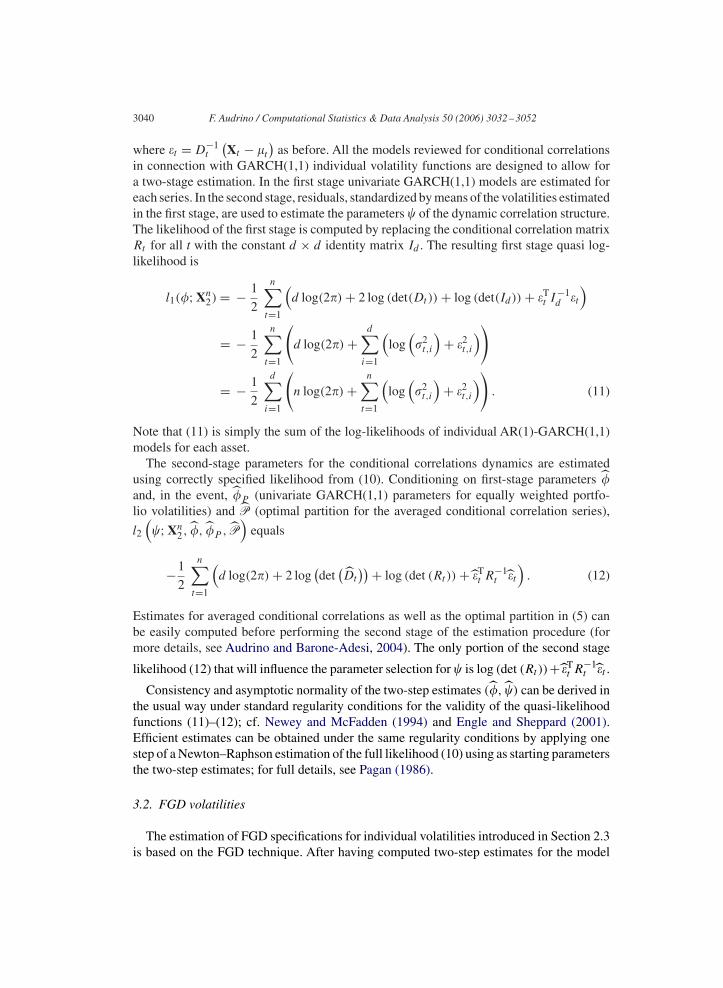
in connection with GARCH(1,1) individual volatility functions are designed to allow fora two-stage estimation. In the first stage univariate GARCH(1,1) models are estimated foreach series. In the second stage, residuals, standardized by means of the volatilities estimatedin the first stage, are used to estimate the parameters � of the dynamic correlation structure.The likelihood of the first stage is computed by replacing the conditional correlation matrixRt for all t with the constant d × d identity matrix Id . The resulting first stage quasi log-likelihood is
l1(�; Xn2) = − 1
2
n∑t=1
(d log(2�) + 2 log (det(Dt )) + log (det(Id)) + �T
t I−1d �t
)= − 1
2
n∑t=1
(d log(2�) +
d∑i=1
(log
(�2
t,i
)+ �2
t,i
))
= − 1
2
d∑i=1
(n log(2�) +
n∑t=1
(log
(�2
t,i
)+ �2
t,i
)). (11)
Note that (11) is simply the sum of the log-likelihoods of individual AR(1)-GARCH(1,1)models for each asset.
The second-stage parameters for the conditional correlations dynamics are estimatedusing correctly specified likelihood from (10). Conditioning on first-stage parameters �and, in the event, �P (univariate GARCH(1,1) parameters for equally weighted portfo-lio volatilities) and P (optimal partition for the averaged conditional correlation series),
l2
(�; Xn
2, �, �P , P)
equals
−1
2
n∑t=1
(d log(2�) + 2 log
(det
(Dt
))+ log (det (Rt )) + �Tt R−1
t �t)
. (12)
Estimates for averaged conditional correlations as well as the optimal partition in (5) canbe easily computed before performing the second stage of the estimation procedure (formore details, see Audrino and Barone-Adesi, 2004). The only portion of the second stage
likelihood (12) that will influence the parameter selection for � is log (det (Rt ))+ �Tt R−1
t �t .
Consistency and asymptotic normality of the two-step estimates (�, �) can be derived inthe usual way under standard regularity conditions for the validity of the quasi-likelihoodfunctions (11)–(12); cf. Newey and McFadden (1994) and Engle and Sheppard (2001).Efficient estimates can be obtained under the same regularity conditions by applying onestep of a Newton–Raphson estimation of the full likelihood (10) using as starting parametersthe two-step estimates; for full details, see Pagan (1986).
3.2. FGD volatilities
The estimation of FGD specifications for individual volatilities introduced in Section 2.3is based on the FGD technique. After having computed two-step estimates for the model
F. Audrino / Computational Statistics & Data Analysis 50 (2006) 3032–3052 3041
parameters, we move one step further using FGD for the individual volatility functions. Theestimated time-varying conditional correlation dynamics are kept fixed.
The FGD algorithm used in this paper is the one recently proposed by Audrino andBühlmann (2003) and is described in Appendix A. Note that it is a greedy-stagewise algo-rithm: it never adjusts previously fitted terms. Similarly to Audrino and Bühlmann (2003),in our empirical investigations we choose q = 1 for the number q of lagged variables tobe used as predictors and regression trees with three final nodes as base learner. For theestimation, we use a shrinkage factor = 0.25 in (A.3).
3.3. Data
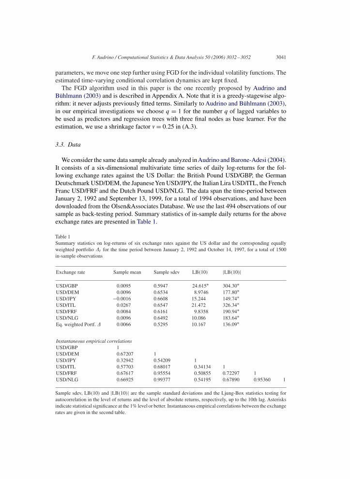
We consider the same data sample already analyzed inAudrino and Barone-Adesi (2004).It consists of a six-dimensional multivariate time series of daily log-returns for the fol-lowing exchange rates against the US Dollar: the British Pound USD/GBP, the GermanDeutschmark USD/DEM, the JapaneseYen USD/JPY, the Italian Lira USD/ITL, the FrenchFranc USD/FRF and the Dutch Pound USD/NLG. The data span the time-period betweenJanuary 2, 1992 and September 13, 1999, for a total of 1994 observations, and have beendownloaded from the Olsen&Associates Database. We use the last 494 observations of oursample as back-testing period. Summary statistics of in-sample daily returns for the aboveexchange rates are presented in Table 1.
Table 1Summary statistics on log-returns of six exchange rates against the US dollar and the corresponding equallyweighted portfolio �t for the time period between January 2, 1992 and October 14, 1997, for a total of 1500in-sample observations
Exchange rate Sample mean Sample sdev LB(10) |LB(10)|
USD/GBP 0.0095 0.5947 24.615∗ 304.30∗USD/DEM 0.0096 0.6534 8.9746 177.80∗USD/JPY −0.0016 0.6608 15.244 149.74∗USD/ITL 0.0267 0.6547 21.472 326.34∗USD/FRF 0.0084 0.6161 9.8358 190.94∗USD/NLG 0.0096 0.6492 10.086 183.64∗Eq. weighted Portf. � 0.0066 0.5295 10.167 136.09∗
Instantaneous empirical correlationsUSD/GBP 1USD/DEM 0.67207 1USD/JPY 0.32942 0.54209 1USD/ITL 0.57703 0.68017 0.34134 1USD/FRF 0.67617 0.95554 0.50855 0.72297 1USD/NLG 0.66925 0.99377 0.54195 0.67890 0.95360 1
Sample sdev, LB(10) and |LB(10)| are the sample standard deviations and the Ljung-Box statistics testing forautocorrelation in the level of returns and the level of absolute returns, respectively, up to the 10th lag. Asterisksindicate statistical significance at the 1% level or better. Instantaneous empirical correlations between the exchangerates are given in the second table.
3042 F. Audrino / Computational Statistics & Data Analysis 50 (2006) 3032–3052
Sample means for the different exchange rates are very similar. The USD/JPY ex-change rate shows a negative mean return that is attributable to a strong Japanese Yenduring the in-sample period considered. The sample standard deviations exhibited by allexchange rates are similar. As expected, the sample standard deviation is reduced byconstructing the equally weighted portfolio. The Ljung-Box statistics LB(10) testing forautocorrelations in the level of returns up to the 10th order show, in all cases exceptfor the USD/GBP exchange rates, no significant presence of autocorrelation in daily ex-change rate returns. The |LB(10)| statistics testing the null hypothesis of dependency ofthe absolute exchange rate and portfolio returns are all highly significant. The USD/DEM,USD/FRF and USD/NLG exchange rate returns exhibit the highest sample correlationswith each other, indicating a strong dependence structure among the exchange rates ofthese markets, whereas the lowest correlations are those with the USD/JPY exchange ratereturns.
4. Empirical results
We test here the conditional covariance matrix estimates from the different model speci-fication fits introduced in Section 2 on the six-dimensional exchange-rate return time seriesintroduced in Section 3.3. We are particularly interested in:
(i) comparing the predictive power of the FGD against the simple GARCH(1,1) specifica-tion for the volatility dynamics in the different model settings for conditional correla-tions;
(ii) evaluating whether general FGD volatilities in the (possibly mis-specified) CCC settingare able to incorporate some non-linear cross-dependence effects and, consequently, tocorrect for eventual inaccuracies of conditional covariance estimates and predictions.
This is done by comparing several goodness-of-fit statistics at the multivariate and univariateportfolio levels. Moreover, we carry out statistical t-type and sign-type tests on differencesof performance terms for the null hypothesis of equal predictive ability (EPA) betweenfits from (i) the two volatility specifications (GARCH(1,1) and FGD) in the different con-ditional correlation settings and (ii) the CCC-FGD model against the multiple alternativeconditional correlation GARCH(1,1) models.
4.1. Estimated in-sample residuals
We analyze first the standardized residuals from the different model fits. The compari-son is performed using the same goodness-of-fit criterion already proposed by Engle andSheppard (2001).
Consider the standardized residuals Zt = �−1t
(Xt − �t
)in (1). From the assumption
(A.1) of the model, cross products ZtZTt are uncorrelated over time. It is therefore natural
to check whether the estimated cross products are uncorrelated over time.We compute the percentages of rejected classical Ljung-Box tests investigating whether
there is excess serial correlation in the squares and cross products of standardized residuals
F. Audrino / Computational Statistics & Data Analysis 50 (2006) 3032–3052 3043
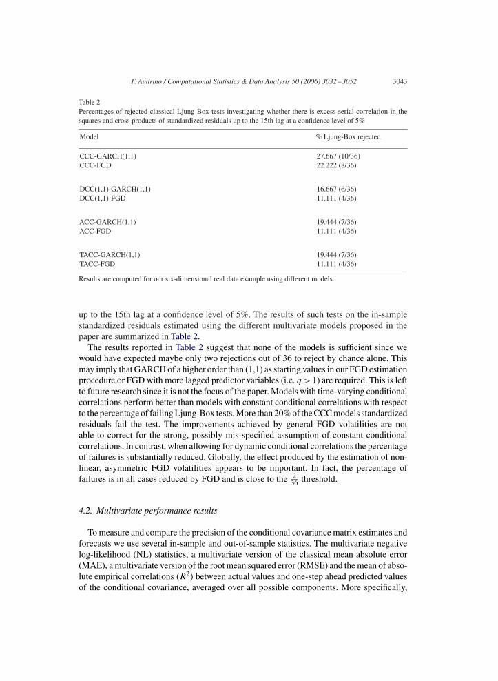
Table 2Percentages of rejected classical Ljung-Box tests investigating whether there is excess serial correlation in thesquares and cross products of standardized residuals up to the 15th lag at a confidence level of 5%
Model % Ljung-Box rejected
CCC-GARCH(1,1) 27.667 (10/36)CCC-FGD 22.222 (8/36)
DCC(1,1)-GARCH(1,1) 16.667 (6/36)DCC(1,1)-FGD 11.111 (4/36)
ACC-GARCH(1,1) 19.444 (7/36)ACC-FGD 11.111 (4/36)
TACC-GARCH(1,1) 19.444 (7/36)TACC-FGD 11.111 (4/36)
Results are computed for our six-dimensional real data example using different models.
up to the 15th lag at a confidence level of 5%. The results of such tests on the in-samplestandardized residuals estimated using the different multivariate models proposed in thepaper are summarized in Table 2.
The results reported in Table 2 suggest that none of the models is sufficient since wewould have expected maybe only two rejections out of 36 to reject by chance alone. Thismay imply that GARCH of a higher order than (1,1) as starting values in our FGD estimationprocedure or FGD with more lagged predictor variables (i.e. q > 1) are required. This is leftto future research since it is not the focus of the paper. Models with time-varying conditionalcorrelations perform better than models with constant conditional correlations with respectto the percentage of failing Ljung-Box tests. More than 20% of the CCC models standardizedresiduals fail the test. The improvements achieved by general FGD volatilities are notable to correct for the strong, possibly mis-specified assumption of constant conditionalcorrelations. In contrast, when allowing for dynamic conditional correlations the percentageof failures is substantially reduced. Globally, the effect produced by the estimation of non-linear, asymmetric FGD volatilities appears to be important. In fact, the percentage offailures is in all cases reduced by FGD and is close to the 2
36 threshold.
4.2. Multivariate performance results
To measure and compare the precision of the conditional covariance matrix estimates andforecasts we use several in-sample and out-of-sample statistics. The multivariate negativelog-likelihood (NL) statistics, a multivariate version of the classical mean absolute error(MAE), a multivariate version of the root mean squared error (RMSE) and the mean of abso-lute empirical correlations (R2) between actual values and one-step ahead predicted valuesof the conditional covariance, averaged over all possible components. More specifically,
3044 F. Audrino / Computational Statistics & Data Analysis 50 (2006) 3032–3052
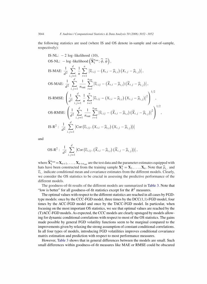
the following statistics are used (where IS and OS denote in-sample and out-of-sample,respectively):
IS-NL: − 2 log -likelihood (10),
OS-NL: − log -likelihood(
Xnout1 ; �, �
),
IS-MAE:1
d2
d∑i,j=1
1
n
n∑t=1
∣∣vt,ij − (Xt,i − �t,i
) (Xt,j − �t,j
)∣∣ ,
OS-MAE:1
d2
d∑i,j=1
1
nout
nout∑t=1
∣∣vt,ij − (Xt,i − �t,i
) (Xt,j − �t,j
)∣∣ ,
IS-RMSE:
⎛⎝ 1
d2
d∑i,j=1
1
n
n∑t=1
∣∣vt,ij − (Xt,i − �t,i
) (Xt,j − �t,j
)∣∣2⎞⎠1/2
,
OS-RMSE:
⎛⎝ 1
d2
d∑i,j=1
1
nout
nout∑t=1
∣∣vt,ij − (Xt,i − �t,i
) (Xt,j − �t,j
)∣∣2⎞⎠1/2
,
IS-R2 : 1
d2
d∑i,j=1
∣∣Cor(vt,ij ,
(Xt,i − �t,i
) (Xt,j − �t,j
))∣∣and
OS-R2 : 1
d2
d∑i,j=1
∣∣Cor(vt,ij ,
(Xt,i − �t,i
) (Xt,j − �t,j
))∣∣ ,
where Xnout1 =Xn+1, . . . , Xn+nout are the test data and the parameter estimates equipped with
hats have been constructed from the training sample Xn1 = X1, . . . , Xn. Note that �t,· and
vt,· indicate conditional mean and covariance estimates from the different models. Clearly,we consider the OS statistics to be crucial in assessing the predictive performance of thedifferent models.
The goodness-of-fit results of the different models are summarized in Table 3. Note that“low is better” for all goodness-of-fit statistics except for the R2 measures.
The optimal values with respect to the different statistics are reached in all cases by FGD-type models: once by the CCC-FGD model, three times by the DCC(1,1)-FGD model, fourtimes by the ACC-FGD model and once by the TACC-FGD model. In particular, whenfocusing on the most important OS statistics, we see that optimal values are reached by the(T)ACC-FGD models. As expected, the CCC models are clearly upstaged by models allow-ing for dynamic conditional correlations with respect to most of the OS statistics. The gainsmade possible by general FGD volatility functions seem to be marginal compared to theimprovements given by relaxing the strong assumption of constant conditional correlations.In all four types of models, introducing FGD volatilities improves conditional covariancematrix estimation and prediction with respect to most performance measures.
However, Table 3 shows that in general differences between the models are small. Suchsmall differences within goodness-of-fit measures like MAE or RMSE could be obscured
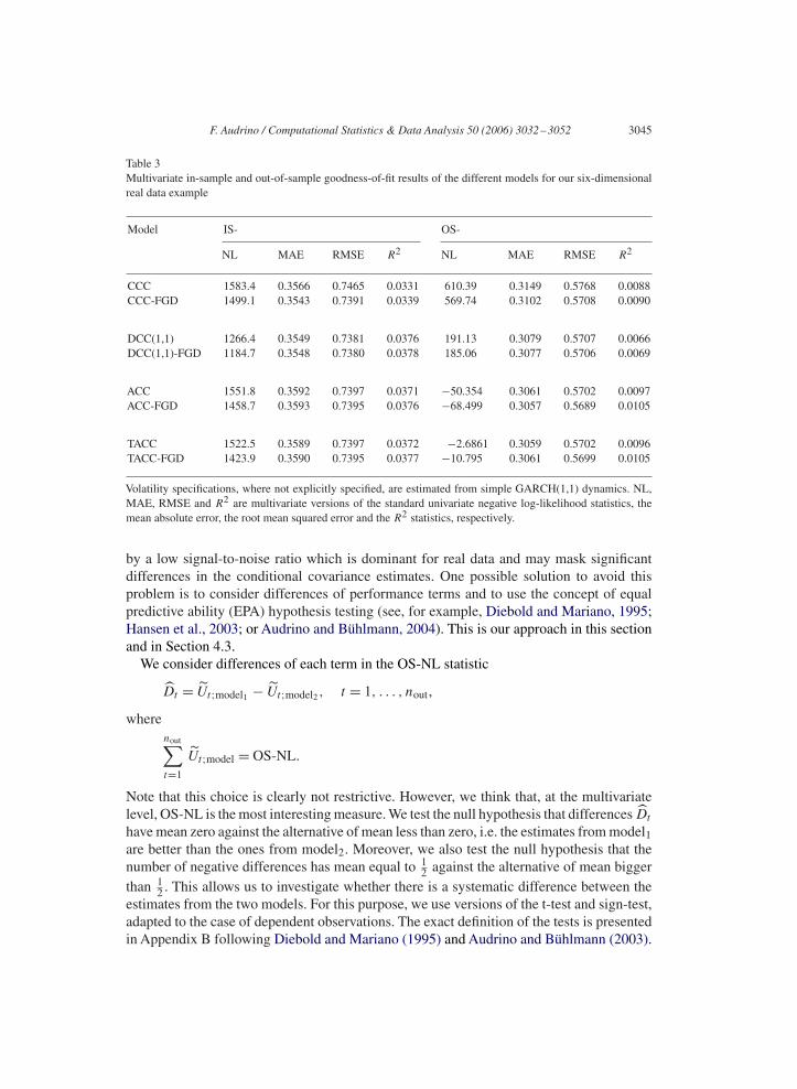
F. Audrino / Computational Statistics & Data Analysis 50 (2006) 3032–3052 3045
Table 3Multivariate in-sample and out-of-sample goodness-of-fit results of the different models for our six-dimensionalreal data example
Model IS- OS-
NL MAE RMSE R2 NL MAE RMSE R2
CCC 1583.4 0.3566 0.7465 0.0331 610.39 0.3149 0.5768 0.0088CCC-FGD 1499.1 0.3543 0.7391 0.0339 569.74 0.3102 0.5708 0.0090
DCC(1,1) 1266.4 0.3549 0.7381 0.0376 191.13 0.3079 0.5707 0.0066DCC(1,1)-FGD 1184.7 0.3548 0.7380 0.0378 185.06 0.3077 0.5706 0.0069
ACC 1551.8 0.3592 0.7397 0.0371 −50.354 0.3061 0.5702 0.0097ACC-FGD 1458.7 0.3593 0.7395 0.0376 −68.499 0.3057 0.5689 0.0105
TACC 1522.5 0.3589 0.7397 0.0372 −2.6861 0.3059 0.5702 0.0096TACC-FGD 1423.9 0.3590 0.7395 0.0377 −10.795 0.3061 0.5699 0.0105
Volatility specifications, where not explicitly specified, are estimated from simple GARCH(1,1) dynamics. NL,MAE, RMSE and R2 are multivariate versions of the standard univariate negative log-likelihood statistics, themean absolute error, the root mean squared error and the R2 statistics, respectively.
by a low signal-to-noise ratio which is dominant for real data and may mask significantdifferences in the conditional covariance estimates. One possible solution to avoid thisproblem is to consider differences of performance terms and to use the concept of equalpredictive ability (EPA) hypothesis testing (see, for example, Diebold and Mariano, 1995;Hansen et al., 2003; or Audrino and Bühlmann, 2004). This is our approach in this sectionand in Section 4.3.
We consider differences of each term in the OS-NL statistic
Dt = Ut;model1 − Ut;model2 , t = 1, . . . , nout,
wherenout∑t=1
Ut;model = OS-NL.
Note that this choice is clearly not restrictive. However, we think that, at the multivariatelevel, OS-NL is the most interesting measure. We test the null hypothesis that differences Dt
have mean zero against the alternative of mean less than zero, i.e. the estimates from model1are better than the ones from model2. Moreover, we also test the null hypothesis that thenumber of negative differences has mean equal to 1
2 against the alternative of mean biggerthan 1
2 . This allows us to investigate whether there is a systematic difference between theestimates from the two models. For this purpose, we use versions of the t-test and sign-test,adapted to the case of dependent observations. The exact definition of the tests is presentedin Appendix B following Diebold and Mariano (1995) and Audrino and Bühlmann (2003).
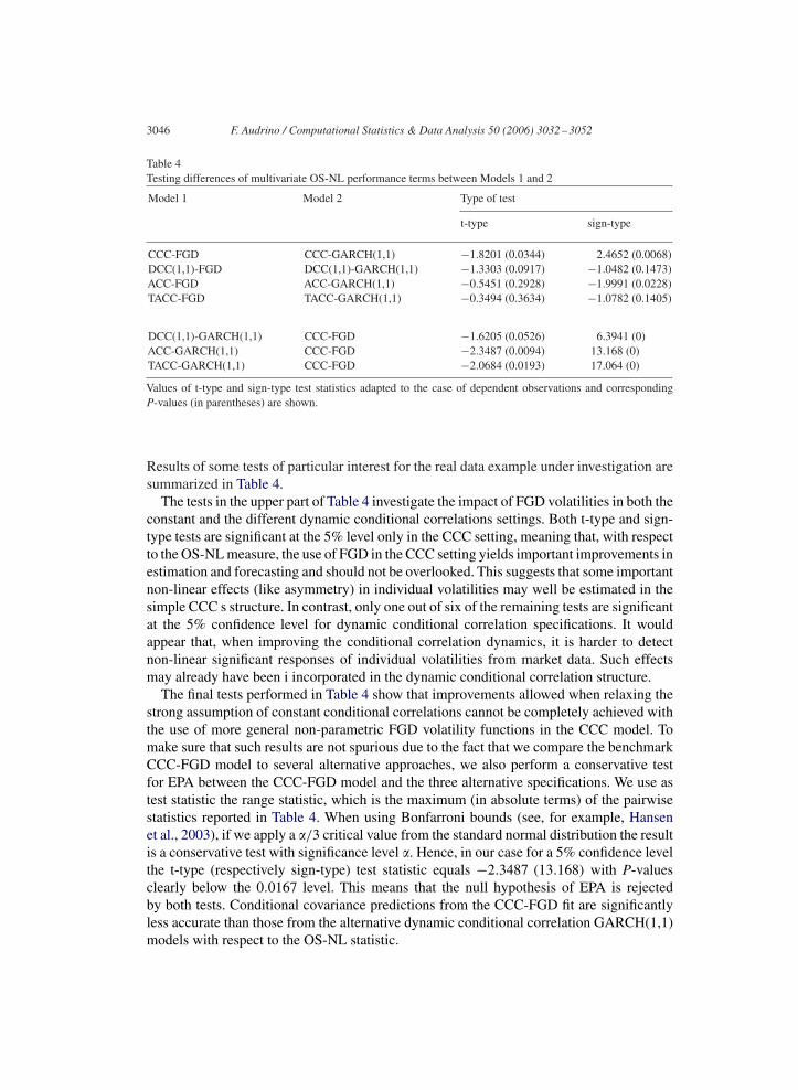
3046 F. Audrino / Computational Statistics & Data Analysis 50 (2006) 3032–3052
Table 4Testing differences of multivariate OS-NL performance terms between Models 1 and 2
Model 1 Model 2 Type of test
t-type sign-type
CCC-FGD CCC-GARCH(1,1) −1.8201 (0.0344) 2.4652 (0.0068)DCC(1,1)-FGD DCC(1,1)-GARCH(1,1) −1.3303 (0.0917) −1.0482 (0.1473)ACC-FGD ACC-GARCH(1,1) −0.5451 (0.2928) −1.9991 (0.0228)TACC-FGD TACC-GARCH(1,1) −0.3494 (0.3634) −1.0782 (0.1405)
DCC(1,1)-GARCH(1,1) CCC-FGD −1.6205 (0.0526) 6.3941 (0)ACC-GARCH(1,1) CCC-FGD −2.3487 (0.0094) 13.168 (0)TACC-GARCH(1,1) CCC-FGD −2.0684 (0.0193) 17.064 (0)
Values of t-type and sign-type test statistics adapted to the case of dependent observations and correspondingP-values (in parentheses) are shown.
Results of some tests of particular interest for the real data example under investigation aresummarized in Table 4.
The tests in the upper part of Table 4 investigate the impact of FGD volatilities in both theconstant and the different dynamic conditional correlations settings. Both t-type and sign-type tests are significant at the 5% level only in the CCC setting, meaning that, with respectto the OS-NL measure, the use of FGD in the CCC setting yields important improvements inestimation and forecasting and should not be overlooked. This suggests that some importantnon-linear effects (like asymmetry) in individual volatilities may well be estimated in thesimple CCC s structure. In contrast, only one out of six of the remaining tests are significantat the 5% confidence level for dynamic conditional correlation specifications. It wouldappear that, when improving the conditional correlation dynamics, it is harder to detectnon-linear significant responses of individual volatilities from market data. Such effectsmay already have been i incorporated in the dynamic conditional correlation structure.
The final tests performed in Table 4 show that improvements allowed when relaxing thestrong assumption of constant conditional correlations cannot be completely achieved withthe use of more general non-parametric FGD volatility functions in the CCC model. Tomake sure that such results are not spurious due to the fact that we compare the benchmarkCCC-FGD model to several alternative approaches, we also perform a conservative testfor EPA between the CCC-FGD model and the three alternative specifications. We use astest statistic the range statistic, which is the maximum (in absolute terms) of the pairwisestatistics reported in Table 4. When using Bonfarroni bounds (see, for example, Hansenet al., 2003), if we apply a �/3 critical value from the standard normal distribution the resultis a conservative test with significance level �. Hence, in our case for a 5% confidence levelthe t-type (respectively sign-type) test statistic equals −2.3487 (13.168) with P-valuesclearly below the 0.0167 level. This means that the null hypothesis of EPA is rejectedby both tests. Conditional covariance predictions from the CCC-FGD fit are significantlyless accurate than those from the alternative dynamic conditional correlation GARCH(1,1)models with respect to the OS-NL statistic.
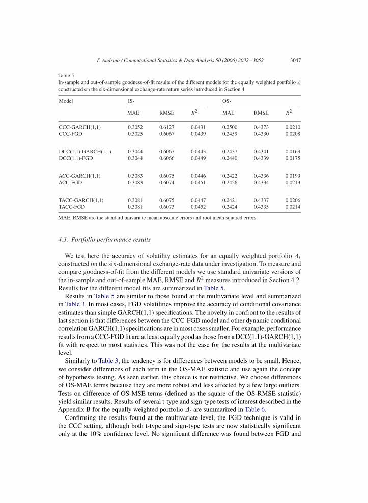
F. Audrino / Computational Statistics & Data Analysis 50 (2006) 3032–3052 3047
Table 5In-sample and out-of-sample goodness-of-fit results of the different models for the equally weighted portfolio �constructed on the six-dimensional exchange-rate return series introduced in Section 4
Model IS- OS-
MAE RMSE R2 MAE RMSE R2
CCC-GARCH(1,1) 0.3052 0.6127 0.0431 0.2500 0.4373 0.0210CCC-FGD 0.3025 0.6067 0.0439 0.2459 0.4330 0.0208
DCC(1,1)-GARCH(1,1) 0.3044 0.6067 0.0443 0.2437 0.4341 0.0169DCC(1,1)-FGD 0.3044 0.6066 0.0449 0.2440 0.4339 0.0175
ACC-GARCH(1,1) 0.3083 0.6075 0.0446 0.2422 0.4336 0.0199ACC-FGD 0.3083 0.6074 0.0451 0.2426 0.4334 0.0213
TACC-GARCH(1,1) 0.3081 0.6075 0.0447 0.2421 0.4337 0.0206TACC-FGD 0.3081 0.6073 0.0452 0.2424 0.4335 0.0214
MAE, RMSE are the standard univariate mean absolute errors and root mean squared errors.
4.3. Portfolio performance results
We test here the accuracy of volatility estimates for an equally weighted portfolio �t
constructed on the six-dimensional exchange-rate data under investigation. To measure andcompare goodness-of-fit from the different models we use standard univariate versions ofthe in-sample and out-of-sample MAE, RMSE and R2 measures introduced in Section 4.2.Results for the different model fits are summarized in Table 5.
Results in Table 5 are similar to those found at the multivariate level and summarizedin Table 3. In most cases, FGD volatilities improve the accuracy of conditional covarianceestimates than simple GARCH(1,1) specifications. The novelty in confront to the results oflast section is that differences between the CCC-FGD model and other dynamic conditionalcorrelation GARCH(1,1) specifications are in most cases smaller. For example, performanceresults from a CCC-FGD fit are at least equally good as those from a DCC(1,1)-GARCH(1,1)fit with respect to most statistics. This was not the case for the results at the multivariatelevel.
Similarly to Table 3, the tendency is for differences between models to be small. Hence,we consider differences of each term in the OS-MAE statistic and use again the conceptof hypothesis testing. As seen earlier, this choice is not restrictive. We choose differencesof OS-MAE terms because they are more robust and less affected by a few large outliers.Tests on difference of OS-MSE terms (defined as the square of the OS-RMSE statistic)yield similar results. Results of several t-type and sign-type tests of interest described in theAppendix B for the equally weighted portfolio �t are summarized in Table 6.
Confirming the results found at the multivariate level, the FGD technique is valid inthe CCC setting, although both t-type and sign-type tests are now statistically significantonly at the 10% confidence level. No significant difference was found between FGD and
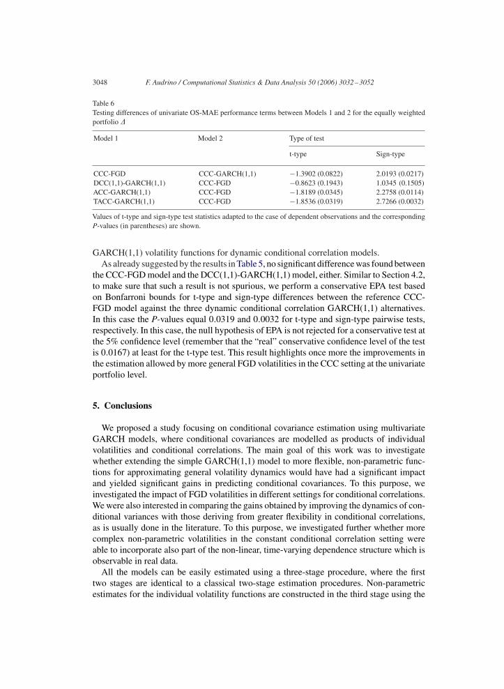
3048 F. Audrino / Computational Statistics & Data Analysis 50 (2006) 3032–3052
Table 6Testing differences of univariate OS-MAE performance terms between Models 1 and 2 for the equally weightedportfolio �
Model 1 Model 2 Type of test
t-type Sign-type
CCC-FGD CCC-GARCH(1,1) −1.3902 (0.0822) 2.0193 (0.0217)DCC(1,1)-GARCH(1,1) CCC-FGD −0.8623 (0.1943) 1.0345 (0.1505)ACC-GARCH(1,1) CCC-FGD −1.8189 (0.0345) 2.2758 (0.0114)TACC-GARCH(1,1) CCC-FGD −1.8536 (0.0319) 2.7266 (0.0032)
Values of t-type and sign-type test statistics adapted to the case of dependent observations and the correspondingP-values (in parentheses) are shown.
GARCH(1,1) volatility functions for dynamic conditional correlation models.As already suggested by the results in Table 5, no significant difference was found between
the CCC-FGD model and the DCC(1,1)-GARCH(1,1) model, either. Similar to Section 4.2,to make sure that such a result is not spurious, we perform a conservative EPA test basedon Bonfarroni bounds for t-type and sign-type differences between the reference CCC-FGD model against the three dynamic conditional correlation GARCH(1,1) alternatives.In this case the P-values equal 0.0319 and 0.0032 for t-type and sign-type pairwise tests,respectively. In this case, the null hypothesis of EPA is not rejected for a conservative test atthe 5% confidence level (remember that the “real” conservative confidence level of the testis 0.0167) at least for the t-type test. This result highlights once more the improvements inthe estimation allowed by more general FGD volatilities in the CCC setting at the univariateportfolio level.
5. Conclusions
We proposed a study focusing on conditional covariance estimation using multivariateGARCH models, where conditional covariances are modelled as products of individualvolatilities and conditional correlations. The main goal of this work was to investigatewhether extending the simple GARCH(1,1) model to more flexible, non-parametric func-tions for approximating general volatility dynamics would have had a significant impactand yielded significant gains in predicting conditional covariances. To this purpose, weinvestigated the impact of FGD volatilities in different settings for conditional correlations.We were also interested in comparing the gains obtained by improving the dynamics of con-ditional variances with those deriving from greater flexibility in conditional correlations,as is usually done in the literature. To this purpose, we investigated further whether morecomplex non-parametric volatilities in the constant conditional correlation setting wereable to incorporate also part of the non-linear, time-varying dependence structure which isobservable in real data.
All the models can be easily estimated using a three-stage procedure, where the firsttwo stages are identical to a classical two-stage estimation procedures. Non-parametricestimates for the individual volatility functions are constructed in the third stage using the
F. Audrino / Computational Statistics & Data Analysis 50 (2006) 3032–3052 3049
functional gradient descent (FGD) technique in Audrino and Bühlmann (2003) where the(time-varying) conditional correlation dynamics remain fixed.
The empirical evidence we collected by testing the different models on a six-dimensionalreal exchange-rate data sample served two purposes. First, it helped us demonstrate thestrong predictive power of FGD volatilities in the CCC setting, suggesting that non-lineareffects in volatilities cannot be neglected in this simple context for conditions correlations.Secondly, it proved the ability of the FGD technique in the CCC setting to partially close thegap to more structured models featuring time-varying correlations for univariate portfolioapplications.
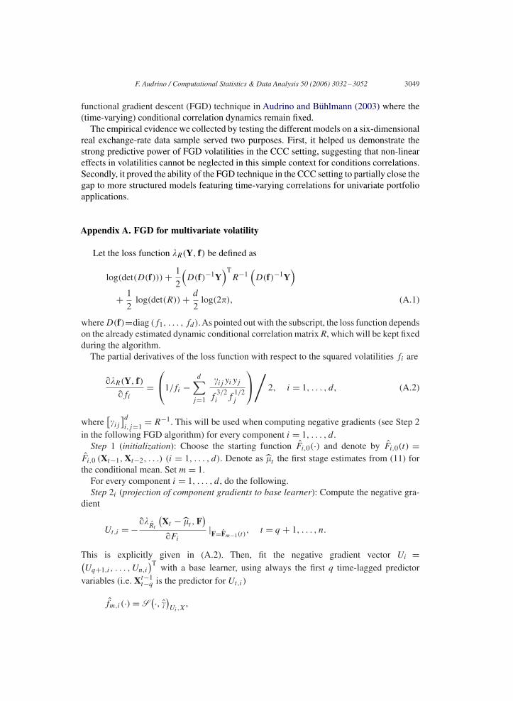
Appendix A. FGD for multivariate volatility
Let the loss function �R(Y, f) be defined as
log(det(D(f))) + 1
2
(D(f)−1Y
)TR−1
(D(f)−1Y
)+ 1
2log(det(R)) + d
2log(2�), (A.1)
where D(f)=diag (f1, . . . , fd).As pointed out with the subscript, the loss function dependson the already estimated dynamic conditional correlation matrix R, which will be kept fixedduring the algorithm.
The partial derivatives of the loss function with respect to the squared volatilities fi are
��R(Y, f)�fi
=⎛⎝1/fi −
d∑j=1
ij yiyj
f3/2i f
1/2j
⎞⎠/ 2, i = 1, . . . , d, (A.2)
where[ij
]di,j=1
= R−1. This will be used when computing negative gradients (see Step 2in the following FGD algorithm) for every component i = 1, . . . , d.
Step 1 (initialization): Choose the starting function Fi,0(·) and denote by Fi,0(t) =Fi,0 (Xt−1, Xt−2, . . .) (i = 1, . . . , d). Denote as �t the first stage estimates from (11) forthe conditional mean. Set m = 1.
For every component i = 1, . . . , d, do the following.Step 2i (projection of component gradients to base learner): Compute the negative gra-
dient
Ut,i = −��Rt
(Xt − �t , F
)�Fi
|F=Fm−1(t), t = q + 1, . . . , n.
This is explicitly given in (A.2). Then, fit the negative gradient vector Ui =(Uq+1,i , . . . , Un,i
)T with a base learner, using always the first q time-lagged predictorvariables (i.e. Xt−1
t−q is the predictor for Ut,i)
fm,i(·) = S(·, )
Ui,X,
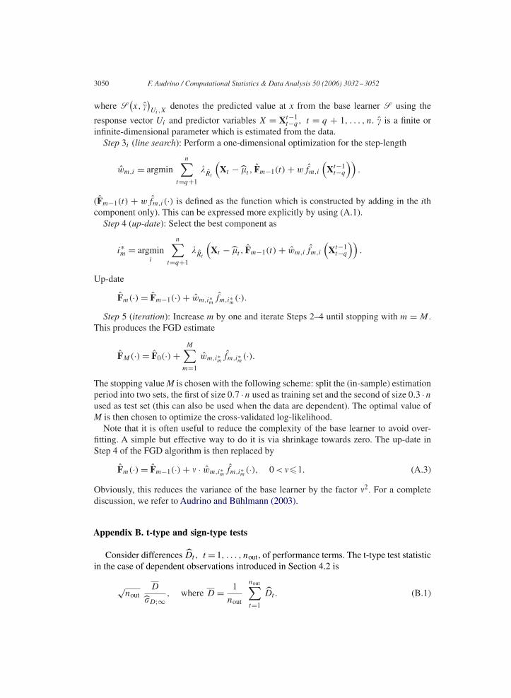
3050 F. Audrino / Computational Statistics & Data Analysis 50 (2006) 3032–3052
where S(x,
)Ui,X
denotes the predicted value at x from the base learner S using the
response vector Ui and predictor variables X = Xt−1t−q, t = q + 1, . . . , n. is a finite or
infinite-dimensional parameter which is estimated from the data.Step 3i (line search): Perform a one-dimensional optimization for the step-length
wm,i = argminn∑
t=q+1
�Rt
(Xt − �t , Fm−1(t) + wfm,i
(Xt−1
t−q
)).
(Fm−1(t) + wfm,i(·) is defined as the function which is constructed by adding in the ithcomponent only). This can be expressed more explicitly by using (A.1).
Step 4 (up-date): Select the best component as
i∗m = argmini
n∑t=q+1
�Rt
(Xt − �t , Fm−1(t) + wm,i fm,i
(Xt−1
t−q
)).
Up-date
Fm(·) = Fm−1(·) + wm,i∗mfm,i∗m(·).Step 5 (iteration): Increase m by one and iterate Steps 2–4 until stopping with m = M .
This produces the FGD estimate
FM(·) = F0(·) +M∑
m=1
wm,i∗mfm,i∗m(·).
The stopping value M is chosen with the following scheme: split the (in-sample) estimationperiod into two sets, the first of size 0.7 ·n used as training set and the second of size 0.3 ·nused as test set (this can also be used when the data are dependent). The optimal value ofM is then chosen to optimize the cross-validated log-likelihood.
Note that it is often useful to reduce the complexity of the base learner to avoid over-fitting. A simple but effective way to do it is via shrinkage towards zero. The up-date inStep 4 of the FGD algorithm is then replaced by
Fm(·) = Fm−1(·) + · wm,i∗mfm,i∗m(·), 0 < �1. (A.3)
Obviously, this reduces the variance of the base learner by the factor 2. For a completediscussion, we refer to Audrino and Bühlmann (2003).
Appendix B. t-type and sign-type tests
Consider differences Dt , t = 1, . . . , nout, of performance terms. The t-type test statisticin the case of dependent observations introduced in Section 4.2 is
√nout
D
�D;∞, where D = 1
nout
nout∑t=1
Dt . (B.1)
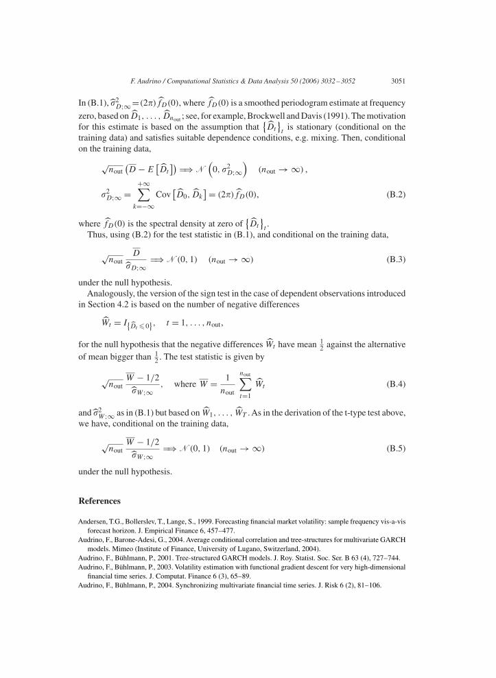
F. Audrino / Computational Statistics & Data Analysis 50 (2006) 3032–3052 3051
In (B.1), �2D;∞=(2�)fD(0), where fD(0) is a smoothed periodogram estimate at frequency
zero, based on D1, . . . , Dnout ; see, for example, Brockwell and Davis (1991). The motivationfor this estimate is based on the assumption that
{Dt
}t
is stationary (conditional on thetraining data) and satisfies suitable dependence conditions, e.g. mixing. Then, conditionalon the training data,
√nout
(D − E
[Dt
]) ⇒ N(
0, �2D;∞
)(nout → ∞) ,
�2D;∞ =
+∞∑k=−∞
Cov[D0, Dk
]= (2�)fD(0), (B.2)
where fD(0) is the spectral density at zero of{Dt
}t.
Thus, using (B.2) for the test statistic in (B.1), and conditional on the training data,
√nout
D
�D;∞⇒ N(0, 1) (nout → ∞) (B.3)
under the null hypothesis.Analogously, the version of the sign test in the case of dependent observations introduced
in Section 4.2 is based on the number of negative differences
Wt = I{Dt �0}, t = 1, . . . , nout,
for the null hypothesis that the negative differences Wt have mean 12 against the alternative
of mean bigger than 12 . The test statistic is given by
√nout
W − 1/2
�W ;∞, where W = 1
nout
nout∑t=1
Wt (B.4)
and �2W ;∞ as in (B.1) but based on W1, . . . , WT . As in the derivation of the t-type test above,
we have, conditional on the training data,
√nout
W − 1/2
�W ;∞⇒ N(0, 1) (nout → ∞) (B.5)
under the null hypothesis.
References
Andersen, T.G., Bollerslev, T., Lange, S., 1999. Forecasting financial market volatility: sample frequency vis-a-visforecast horizon. J. Empirical Finance 6, 457–477.
Audrino, F., Barone-Adesi, G., 2004. Average conditional correlation and tree-structures for multivariate GARCHmodels. Mimeo (Institute of Finance, University of Lugano, Switzerland, 2004).
Audrino, F., Bühlmann, P., 2001. Tree-structured GARCH models. J. Roy. Statist. Soc. Ser. B 63 (4), 727–744.Audrino, F., Bühlmann, P., 2003. Volatility estimation with functional gradient descent for very high-dimensional
financial time series. J. Computat. Finance 6 (3), 65–89.Audrino, F., Bühlmann, P., 2004. Synchronizing multivariate financial time series. J. Risk 6 (2), 81–106.

3052 F. Audrino / Computational Statistics & Data Analysis 50 (2006) 3032–3052
Baur, D., 2003. A flexible dynamic correlation model. Mimeo (Joint Research Center, Ispra, Italy, 2003).Beckaert, G., Wu, G., 2000. Asymmetric volatility and risk in equity markets. Rev. Financial Stud. 13, 1–42.Black, F., 1976. Studies in stock price volatility changes. Proceedings of the American Statistical Association,
Business and Economic Statistics Section, pp .177–181.Bollerslev, T., 1986. Generalized autoregressive conditional heteroscedasticity. J. Econometrics 31, 307–327.Bollerslev, T., 1990. Modelling the coherence in short-run nominal exchange rates: a multivariate generalized
ARCH model. Rev. Econom. Statist. 72, 498–505.Campbell, J.Y., Hentschel, L., 1992. No news is good news: an asymmetric model of changing volatility in stock
returns. J. Financial Econom. 31, 281–318.Cappiello, L., Engle, R.F., Sheppard, K., 2003. Asymmetric dynamics in the correlations of global equity and bond
returns. Mimeo (University of California, San Diego, 2003).Christie, A.A., 1982. The stochastic behavior of common stock variances-value, leverage and interest rates effects.
J. Financial Econom. 10, 407–432.Diebold, F.X., Mariano, R.S., 1995. Comparing predictive accuracy. J. Business Econom. Statist. 13, 253–263.Engle, R.F., 2002. Dynamic conditional correlation—a simple class of multivariate GARCH models. J. Business
Econom. Statist. 20, 339–350.Engle, R.F., Sheppard, K., 2001. Theoretical and empirical properties of dynamic conditional correlation
multivariate GARCH. Mimeo (University of California, San Diegom, 2001).Errunza, V.K.H., Hung, M.-W., 1999. Can the gains from international diversification be achieved without trading
abroad? J. Finance 54, 2075–2107.Hansen, P.R., Lunde, A., 2002. A forecast comparison of volatility models: does anything beat a GARCH(1,1)?
Mimeo (Department of Economics, Brown University, 2002).Hansen, P.R., Lunde,A., Nason, J.M., 2003. Choosing the best volatility models: the model confidence set approach.
Oxford Bull. Econom. Statist. 65, 839–861.Kroner, K.F., Ng, V.K., 1998. Modeling asymmetric comovements of asset returns. Rev. Financial Stud. 11 (4),
817–844.Ledoit, O., Santa-Clara, P., Wolf, M., 2003. Flexible multivariate GARCH modeling with an application to
international stock markets. Rev. Econom. Statist. 85 (3), 735–747.Lee, T., Saltoglu, B., 2001. Evaluating the predictive performance of value-at-risk models in emerging markets: a
reality check. Mimeo (Department of Economics, University of California, Riverside, 2001).Newey, W.K., McFadden, D., 1994. Large sample estimation and hypothesis testing. Handbook of Econometrics,
vol. 4. North-Holland, Amsterdam, pp. 2111–2245.Pagan, A., 1986. Two stage and related estimators and their applications. Rev. Econom. Stud. 53 (4), 517–538.Pelletier, D., 2004. Regime switching for dynamic correlations. Forthcoming in the Journal of Econometrics.Tse, Y.K., 2000. A test for constant correlations in a multivariate GARCH model. J. Econometrics 98, 107–127.Tse,Y., Tsui, A., 2002. A multivariate GARCH model with time-varying correlations. J. Business Econom. Statist.
20, 351–362.Wu, G., 2001. The determinants of asymmetric volatility. Rev. Financial Stud. 14, 837–859.