the impact of capital flows on real exchange rates in ... · the impact of capital flows on real...
TRANSCRIPT

The Impact of Capital Flows on Real
Exchange rates in South Africa
MISHI SYDEN
(200705942)
A dissertation submitted in fulfillment of the requirements for the degree
MASTER OF COMMERCE
ECONOMICS
in the
Faculty of Management and Commerce
at the
University of Fort Hare
South Africa
East London
December 2012
SUPERVISOR: PROFESSOR A. TSEGAYE

i
ABSTRACT
The neoclassical theory suggests that free flows of external capital should be
equilibrating and thereby facilitating smoothening of an economy's consumption or
production patterns. South Africa has a very low savings rate, making it highly
dependent on capital inflows which create instability and volatility in global markets. A
policy dilemma is undoubtedly evident: capital inflows help to cater for the domestic low
savings and at the same time the inflows pose instability, a threat on competitiveness
and volatility challenges to the same economy due to their impact on exchange rates.
The question is: are all forms of capital flows equally destabilizing?
Since studies based on South Africa considered only the relationship between
aggregate capital flows and real exchange rate, modelling individual components of
capital flows could enlighten policy formulation even further. The composition of the
flows and their effects on the composition of aggregate demand determine the evolution
of real exchange rate response to surges in capital flows.
Through co-integration and vector error correction modelling techniques applied to
South African data between 1990 and 2010, the study found out that foreign portfolio
investment exerts the greatest appreciation effect on the South African real exchange
rate, followed by other investment and finally foreign direct investment. Thus the impact
of capital flows on real exchange rate in South Africa differs by type of capital. This
presents varied policy implications.

ii
DECLARATIONS
On originality of work
I, the undersigned, Mishi Syden student Number 200705942, hereby declare that the
dissertation is my own original work, and that it has not been submitted, and will not be
presented at any other University for a similar or any other degree award.
Date:………………………
Signature:…………………………………
On plagiarism
I Mishi Syden student number 200705942 hereby declare that I am fully aware of the
University of Fort Hare’s policy on plagiarism and I have taken every precaution to
comply with the regulations.
Signature: ........................
On research ethics clearance
I Mishi Syden student number 200705942 hereby declare that I am fully aware of the
University of Fort Hare’s policy on research ethics and I have taken every precaution to
comply with the regulations. I have obtained an ethical clearance certificate from the
University of Fort Hare’s Research Ethics Committee and my reference number is the
following:..........N/A.................
Signature: ..............................

iii
ACKNOWLEDGEMENTS
Firstly, I would like to thank God, whose hand I continually and sometimes mysteriously felt
upon me as I worked on this study, for making this possible. Many thanks and gratitude goes to
my supervisor and mentor, Professor Asrat Tsegaye for patiently and enthusiastically guiding
and encouraging me throughout the thesis writing process. I have been extremely blessed to
have a supervisor who cared so much about my work, and who responded to my questions and
queries so promptly. Prof., your positive outlook and confidence in my research inspired me and
gave me confidence and your careful editing contributed enormously to the production of this
thesis. I would also like to thank all the members of staff at University of Fort Hare, Department
of Economics for their support.
I must express my gratitude to Lilymore Mudziwapasi, my confidante, for her continued support
and encouragement. I also thank my friends Hlanganani Siqondile Sibanda, Sibanisezwe
Khumalo, Nomfundo Vacu, Forget Kapingura, Tendai Chimucheka, Admire Mthombeni, among
many others for their support and inspiration. I was continually amazed by their willingness to
proof read countless pages and varied comments and words of encouragement throughout the
journey. Any typos that remain are my responsibility.
I am indebted to my parents, Mrs. Theresa Mishi and the late Mr. Tapfumanei Mishi for, without
their love, guidance and provisions I would not have reached this far. I am grateful to the
patience of my mother, and siblings (and their families) and many other relatives who
experienced all of the ups and downs of my research. Many thanks go to Mr. Ezekiel and Mrs.
Autilia Gororo’s family; Mr. Norest Madih and wife; for they continuously spurred me on.
Completing this work would have been all the more difficult were it not for the support provided
by GMRDC through fee waiver facility; the Economic Research of Southern Africa (ERSA) to
attend various conferences/ working groups, and interact with so many people broadening my
reasoning. Special mention goes to the 2012 Second Monetary Policy and Macroeconomic
modelling Conference participants who encouraged and reenergised my effort on the thesis.
Those people/bodies, such as the Downtown East London and Gonubie Churches of Christ,
Students Economic Review Assembly at UFH among other student societies and African
Monitor (where I got an opportunity as Research Intern), that provided a much needed form of
escape from my studies, also deserve thanks for helping me keep things in perspective.

iv
DEDICATION
To My Parents; Lily and my siblings

i
TABLE OF CONTENTS ABSTRACT .......................................................................................................................................... i
DECLARATIONS ............................................................................................................................... ii
On originality of work ......................................................................................................................... ii
On plagiarism ....................................................................................................................................... ii
On research ethics clearance .............................................................................................................. ii
ACKNOWLEDGEMENTS ................................................................................................................ iii
DEDICATION ..................................................................................................................................... iv
LIST OF FIGURES ............................................................................................................................ iv
LIST OF TABLES .............................................................................................................................. iv
ACRONYMS AND ABBREVIATIONS ............................................................................................. v
CHAPTER 1: INTRODUCTION AND BACKGROUND OF THE STUDY .................................. 1
1.1. Introduction .............................................................................................................................. 1
1.2. Problem Statement ................................................................................................................ 4
1.3. Objectives ................................................................................................................................ 5
1.4. Hypotheses ............................................................................................................................. 6
1.5. Justification for the study ....................................................................................................... 6
1.6. Organisation of the study ...................................................................................................... 7
CHAPTER 2: OVERVIEW OF SOUTH AFRICA’S FOREIGN EXCHANGE MARKETS AND
THE BOP’S CAPITAL ACCOUNT ................................................................................................... 9
2.1. Introduction .............................................................................................................................. 9
2.2. Overview of the South African Foreign Exchange Markets ........................................... 10
2.2.3. Foreign Exchange rates .................................................................................................. 10
2.3.1. Exchange controls in South Africa- background ......................................................... 13
2.2.3. South Africa’s Exchange rate policy evolution post 1994 .......................................... 15
2.2.4. Exchange rates trends ..................................................................................................... 16
2.3. Overview of the South African Balance of Payment Accounts: Capital Account ....... 20
2.3.1. Capital Account Liberalisation process: content and sequencing ............................ 21
2.3.2. Liberalising the Capital Account (external financial liberalisation) ............................ 22
2.3.3. Prasad-Rajan (P-R) Pragmatic Approach to Capital Account Liberalisation .......... 23
2.3.4. Composition and Behaviour of Capital Flows .............................................................. 28

ii
2.3.5. Capital Account and Exchange rates ............................................................................ 31
2.4. Summary and Analysis ........................................................................................................ 33
CHAPTER 3: LITERATURE REVIEW .......................................................................................... 35
3.1. Introduction ................................................................................................................................ 35
3.2. Theoretical Literature ............................................................................................................... 35
3.2.1. Traditional Theories ......................................................................................................... 36
3.2.2. Modern Theories ................................................................................................................. 40
3.2.3. The Fisher Effect (Interest Rate Factor) .............................................................................. 47
3.3. Empirical Evidence ................................................................................................................... 50
3.3.1. Evidence from Developed Economies .......................................................................... 51
3.3.2. Evidence from Emerging Market and Developing Economies .................................. 52
3.3.3. Evidence from South Arica ............................................................................................. 60
3.3.4. Hypothesized link between foreign exchange markets and the capital account ............... 62
3.4. Assessment of Literature ........................................................................................................ 63
CHAPTER 4: RESEARCH METHODOLOGY ............................................................................. 65
4.1. Introduction ............................................................................................................................ 65
4.2. Model Specification .............................................................................................................. 65
4.3. Data Sources and Definition of Variables ......................................................................... 67
4.3.1. Real Effective Exchange Rate ............................................................................................ 67
4.3.2. Government spending .......................................................................................................... 67
4.3.3. Capital flows ........................................................................................................................... 68
4.3.4. Productivity gap/ technical progress................................................................................... 68
4.3.5. Terms of trade ....................................................................................................................... 69
4.3.6. Trade policy (trade openness) ........................................................................................ 69
4.3.7. Exchange rate market pressure ..................................................................................... 70
4.4. Data Analysis/ Estimation Techniques .............................................................................. 70
4.4.1 Testing for stationarity/ Unit-root ........................................................................................ 71
4.4.3. Co-integration Modelling ..................................................................................................... 79
4.4.4. Diagnostic checks ................................................................................................................ 86
4.4.4.1. Autocorrelation LM test................................................................................................ 87
4.4.4.2. Heteroskedasticity test ................................................................................................ 87
4.4.4.3. Residual normality test ................................................................................................ 87

iii
4.4.5. Impulse response and variance decomposition .............................................................. 88
4.4.6. Econometric tools ................................................................................................................. 89
4.5. Summary ............................................................................................................................... 89
CHAPTER 5: ESTIMATION AND INTERPRETATION OF RESULTS .................................... 91
5.1. Introduction ............................................................................................................................ 91
5.2. Testing for stationarity/ Unit-root tests .............................................................................. 91
5.2.1. Informal Unit Root Tests .................................................................................................. 92
5.2. Granger Causality Test........................................................................................................ 97
5.3 Co-integration Tests ............................................................................................................. 98
5.3.1. Co-integration test results ............................................................................................... 98
5.4. Diagnostic checks for the VECMs ................................................................................... 107
5.4.1. Autocorrelation LM test ...................................................................................................... 108
5.5. Impulse response and variance decomposition ............................................................ 109
5.5.1. Impulse response analysis ................................................................................................ 109
5.5.2. Variance decomposition .................................................................................................... 110
5.7. Chapter Summary .................................................................................................................. 113
CHAPTER 6: STUDY SUMMARY, CONCLUSIONS, POLICY IMPLICATIONS AND
RECOMMENDATIONS ................................................................................................................. 114
6.1. Summary of the study and Conclusions ......................................................................... 114
6.2. Policy Implications, Recommendations and Lessons for Peer Economies .............. 117
6.3. Limitations of the Study and areas for further research ............................................... 119
REFERENCES ............................................................................................................................... 120
APPENDICES .......................................................................................................................................... A
A1: Data ............................................................................................................................................... A
A2:Correlograms ................................................................................................................................ D
A3: Granger Causality Results ......................................................................................................... E

iv
LIST OF FIGURES Figure 2.1 Real Exchange rates Trends ............................................................................................... 17
Figure 2.2 South Africa’s Net Capital Flows (1990-2010) ................................................................... 29
Figure 2.3 South Africa’s Capital Inflows by type of capital flow (1990-2010) ................................... 30
Figure 3.1 Exchange Rate Determinants ............................................................................................. 48
Figure 3.2 Mundell-Flemming Model ................................................................................................. 49
Figure 5.1: Unit root tests- Graphical analysis at levels ...................................................................... 92
Figure 5.2: Unit root tests- Graphical analysis at first difference ....................................................... 94
Figure 5.3: Co-integration graph ....................................................................................................... 102
Figure 5.4: AR Roots Graph ............................................................................................................... 107
Figure 5.5: Impulse response of REER to its independents ............................................................. 110
Figure 5.6: Variance Decomposition ................................................................................................. 111
LIST OF TABLES
Table 2.1: Comparison between previous and revised weights ......................................................... 12
Table 2.2 Exchange rate Controls ....................................................................................................... 14
Table 2.3: The Weiss chronology of the ideal sequencing of structural economic reform ................ 25
Table 2.4: South African reform sequencing ...................................................................................... 27
Table 5.1: Unit root tests 1994Q1- 2009Q4 at levels and first differences (∆) ................................... 96
Table 5.10: Residual normality test .................................................................................................. 109
Table 5.11: Variance decomposition ................................................................................................ 112
Table 5.2: Granger causality tests ....................................................................................................... 98
Table 5.3: VAR Lag Order Selection Criteria ...................................................................................... 100
Table 5.4: The Pantula principle test results ..................................................................................... 100
Table 5.5: Johansen co-integration rank test results ........................................................................ 102
Table 5.6: VECM results .................................................................................................................... 103
Table 5.7 Vector Error Correction Model ......................................................................................... 106
Table 5.8: Langrange Multiplier test results .................................................................................... 108
Table 5.9: Heteroskedasticity test .................................................................................................... 108

v
ACRONYMS AND ABBREVIATIONS
ADF- Augmented Dickey-Fuller Test
BOP- Balance Of Payment
GDP- Gross Domestic Product
PP- Phillips-Perron
PPP- Purchasing Power Parity
REER- Real Effective Exchange Rate
RER- Real Exchange Rate
RSA- Republic of South Africa
SARB- South African Reserve Bank
US- United States of America
VAR- Vector Autoregressive
VECM- Vector Error Correction Modeling
BESA- Bond Exchange of South Africa
JSE – Johannesburg Stock Exchange
FDI- Foreign Direct Investment
FPI- Foreign Portfolio Investment
OTHERIN- Other Investments
SA- South Africa
BEER- Behavioural Effective Exchange Rate
FEER- Fundamental Effective Exchange Rate

1
CHAPTER 1: INTRODUCTION AND BACKGROUND OF THE
STUDY
1.1. Introduction
Economists, academics, and financial sector operators had long recognised that dealing
with cross boarder capital movements is a difficult policy issue, (Edwards, 1999). The
neoclassical theory suggests that free flow of external capital should be equilibrating
and thereby facilitating smoothening of an economy's consumption or production
patterns. In most countries, the data suggested that capital inflows had supplemented
domestic savings (see, Khatri et al, 1997). Based on this, policymakers in developing
countries more often seek to attract external resources on the assumption that they will
finance savings gaps and promote growth and economic development (Dornbusch,
1998). Unfortunately, these arguments seem to be disconnected from real-world
experiences (Singh, 2003; Icard, 2012), as an influx of the capital tends to pose great
policy dilemma to the same policymakers. Nonetheless, most developing economies
continue to open up their capital accounts with myriad reasons justify.
Developments in an economy’s current account of the balance of payments (BOP)
accounts often indicate its position in attracting foreign resources. Economic reforms in
effort to combat deteriorating economic performance, socio-political challenges or
reflecting goals of new political dispensation often involve financial liberalisation, a
reform bent on attracting external funding. In the context of policy design and
implementation, concern is on results of the reforms, in other words, the correctness
and appropriateness of the contents of the reform pack and their sequencing. Icard
(2012) suggested that momentum in capital account liberalisation should be adapted to
the degree of resilience of the domestic financial sector to external shocks and its ability
to deal with large flows of foreign capital.
South Africa got reintroduced to the international markets in the early 1990’s after an
era of isolation during the apartheid rule. The coming of democratic governance, its
need to heal apartheid injustices, eradicate poverty and create employment saw a
plethora of economic reforms being implemented. The Bill of Rights of 1994 of the new

2
Constitution in South Africa (RSA, 1996), served as a beacon for major economic
reforms that includes: macroeconomic measures of stabilisation; external financial
liberalisation; trade reform; domestic financial liberalisation; and reform of commodity
and labour markets. How these reforms impact capital flow movements, is a question of
interest to academics and policymakers alike. The understanding is essential in the
understanding trends in capital flows, however not the main focus of this current study
but an area of future research. With the inherently disappointing savings culture; tax
reforms, fiscal discipline and the phased approach to exchange control liberalisation
were all set on improving South Africa's attractiveness as a destination for foreign
investment. This form of investment turns out to be a precondition for the new South
Africa in order to address the challenges at hand given the savings culture’s status quo.
According to, Aron, Leape and Thomas (2010), for the greater period since 1994, net
capital inflows have helped to alleviate the key structural constraint of low domestic
savings with the increasing openness to both trade and capital flows, also meaning
South Africa has become vulnerable to new sources of external shocks in the form of
surges and reversals in international capital flows, posing new challenges for
macroeconomic management. Policymakers have been, more often than not, left in the
doldrums with the effects of surges in capital inflows on the domestic currency; see van
der Merwe (2003). One such effect is the pressure on the domestic currency, an
appreciation of the currency when inflows grow.
In light of this, how could an economy enjoy benefits from capital inflows and evade the
related costs? The answer also needs an understanding of the impact different forms of
capital inflows exert on real exchange rates. Across literature, Edwards (1998), Sy and
Tabarraei (2009), Jongwanich (2010), Combes, Kinda and Plane (2011), it is evident
capital inflows results in real exchange rate appreciation. And there is a general view
that the choice of exchange rate regime determines the effect of capital flows on the
real exchange rate. Combes, et al. (2010) stated that, the relationship between the real
exchange rate and capital flows can be seen as depending on the choice of the
exchange rate system. South Africa is currently under floating exchange regime in an
Inflation Targeting (IT) monetary policy framework. The exchange rate flexibility policy is
a stance which, Combes, et al (2011) found to be helpful in dampening appreciation of

3
the real effective exchange rate caused by capital flows. Interestingly: South African
Treasury department (2011) reported that, during 2010 South Africa received net
inflows of R92 billion in liquid foreign capitals, which contributed to upward pressure on
the exchange rate. Adding to that, Icard (2012) pointed out that an influx of foreign
capital leads to currency appreciation under a more flexible exchange rate regime.The
impact of capital flows on real exchange rate is an important and controversial issue for
emerging market economies.
In South Africa different stakeholders from Congress of South African Trade Union
(COSATU) to the Manufacturing Circle1 had identified the strengthening of the Rand
[real] exchange rate as an important factor constraining export growth, the development
of the manufacturing sector and job creation, (Budget Speech Competition, 2011). Real
exchange rate (RER) as a measure of how much, on average, South African produced
goods and services will cost relative to equivalent basket of foreign produced goods and
services, and hence their competitiveness over time becomes a fundamental economic
variable. Exchange rate movements are worthy to curtail in order to mitigate
uncertainties that can impede trade, for example a prolonged real appreciation
associated with large capital inflows can negatively impact on export competitiveness
and investment in the external sector, (see de Paula, 2007). According to Creamer
(February 2011) SARB spent 2% of gross domestic product (GDP), during 2010 on
foreign exchange reserve accumulation in a bid to moderate the effect of different forms
of capital flows on the Rand, which had appreciated strongly in the previous year. This
study seeks to investigate the impact of capital flows on real exchange rate in South
Africa. As in Siourounis (2003), such investigation is motivated by modern international
finance theory which asserts that currencies are as much influenced by capital flows as
by account balances and long-term interest rates.
1 Manufacturing Circle interacts with government and other stakeholders in order to: review, debate and help
formulate policies which will have a positive impact on South Africa’s manufacturing base. The Manufacturing Circle is made up of a number of South Africa’s leading medium to large manufacturing companies from a wide range of industries.

4
1.2. Problem Statement
Developing economies suffer from low savings rates and end up looking abroad for
capital resources. Reuters (2011) noted the South African Finance Minister, Pravin
Gordhan, claiming that South Africa had a very low savings rate, making it highly
dependent on capital flows which are creating instability and volatility in global markets.
A policy dilemma is undoubtedly evident: capital inflows help to cater for the domestic
low savings rates in providing capital resources and at the same time the inflows pose
instability, a threat on competitiveness and volatility challenges to the same economy
due to their impact on exchange rate. An inquiry on the impact of capital flows on real
exchange rate in South Africa will add, to the current literature, necessary policy
considerations and insights to possible policy response tools and mechanism to
accommodate use of foreign capital without much threat on macroeconomic
performance. Gordhan (2010) highlighted on the interconnectedness of investment and
consumption (economic activity) across countries, the changes which would bring real
opportunities for growth and a redistribution of global income and welfare, but also
noted that they are not correlated in predictable ways with exchange rate movements.
This unpredictability of the correlation between flows of capital and the value of the
domestic currency (real exchange rate) forms part of inquiry in this study.
Understanding the relationship (short- and long-term) will help predict the correlation
between these two variables with some degree of certainty.
South Africa was rediscovered by world financial markets in the early 1990’s upon
rescinding of economic sanctions, investor confidence started to build-up in the eve of
democratic governance and looming macroeconomic policy reforms under new
government. It is imperative to note the macroeconomic policy reforms that took place
and their sequencing as these have a great bearing on what later transpired in South
African capital markets and therefore thus on real exchange rates development.
Edwards (1998), noted that most economists agree that liberalisation of the capital
account should take place once trade liberalisation reform has been implemented and
that financial reform (including relaxation of capital controls) should only be
implemented once a modern and efficient bank regulatory and supervisory framework is

5
in place. Which order did these reforms take in South Africa? The results of this
analysis will help gauge if South Africa did it right or it is now experiencing the
consequences of following the wrong sequence in the first place.
The Washington Consensus by Williamson, (1990), as part of the International Best
Practice suggested guidelines on the contents and sequencing of economic reforms.
The recommended sequence is of the order: macroeconomic measures of stabilisation;
reform of domestic commodity and labour markets; tax reform; trade reform; domestic
financial liberalisation; and external financial liberalisation. In South Africa according to
Calitz (2002), reforms took the order: macroeconomic measures of stabilisation;
external financial liberalisation; trade reform; domestic financial liberalisation; and
reform of commodity and labour markets. South Africa did not match the prescribed
sequencing; this has a bearing on the results of the reforms. Liberalisation process has
to consider stability of exchange rates and according to Icard (2012) during the late
1980s and early 1990s, attempts to combine exchange rate stability in Europe with a
progressive liberalisation of capital accounts triggered a series of foreign exchange
crises. .Therefore liberalisation process becomes relevant to the extent of exchange
rate stability Chapter two provides a greater discussion of the sequences and the
possible consequences thereof.
1.3. Objectives
The main objective of this study is to investigate the impact of different forms of capital
flows on real exchange rates in South Africa.
The specific objectives are:
i. to critically review the characteristics and behaviour of capital flows and real
exchange rates in South Africa;
ii. to empirically establish the impact of capital flows on real exchange rates in
South Africa; and
iii. to make conclusions and policy recommendations based on findings of the study

6
1.4. Hypotheses
1. Capital inflows impart negatively on real exchange rates
2. Impact of capital flows on real exchange rate is greatly dependent on the form of
the capital flows
1.5. Justification for the study
According to Pretorius (2002) the opening up of our [South African] markets together
with the well-developed financial system, led to volumes of capital flows never
experienced before. This coincided with increased volatility in the exchange rate of the
Rand. The study investigated the impact of different forms of capital flows on real
exchange rates in South Africa, affording us a better analysis of which type of capital
exerts the greatest impact. Ideally how the substantial flow of capital (necessitated by
liberalisation of financial markets) among countries, influence exchange rates in an
emerging market economy. Capital inflows (Foreign Direct Investment- FDI, Foreign
Portfolio Investment- FPI and Other Investments) tend to appreciate real exchange
rates, lowering interest rates and increasing consumption, investment and growth. As
FDI is more sustainable than the other two (see Berument & Dincer, 2004), which can
easily be reversed leading to financial instabilities, it is of paramount importance to
distinguish the particular effects of each capital flow form on the real exchange rate,
(see also Claessens, Dooley, & Warner (1995); Nowak (2001)). There is great debate
(notably between COSATU and South African Reserve Bank- SARB) on how to deal
with exchange rate appreciation, and what are the forces behind the Rand appreciation
against major currencies. Therefore the need to research on the significance of capital
flows in explaining exchange rates movements. The results found contribute to literature
and inform policy makers about the real variables of concern in addressing pressures
on the exchange rates.
Lartey (2008) argued that the capital inflows have been both beneficial and problematic
posing serious concerns among policymakers because of their potential effects on
macroeconomic stability, the competitiveness of the export sector, and the external

7
viability of the recipient countries. With globalisation, any country would want to improve
or maintain its competitiveness position so as to reap the benefits that come with such
an economic setup. This brings out the importance of real exchange rate in an
economy, more specifically emerging open market economy like South Africa. Real
exchange rate is a key policy variable in South Africa’s open economy, Aron, Elbadawi
and Kahn (1997).
Since other studies based on South Africa, (for example: Aron et al 1997; Simwaka,
2004; Mohamed, 2006; Castilleja-Vargas, 2009), considered only the relationship
between aggregate capital flows and real exchange rate; modelling individual
components of capital flows could enlighten policy formulation even further. Analysis of
the influence of capital flows on exchange rate in South Africa is limited- with particular
concern on the disaggregated capital flows. Gordhan (2011:11) admits that changes in
the volume and direction of capital flows [in South Africa] may be significant over the
year ahead [2012], and are largely beyond the authorities control or influence. This
concern indicates the need to unpack the different types of capital flows and analyse
closely their impact on real exchange rates.
The contradiction in empirical conclusions and current experiences indicates the debate
is raging on and thus calls for further empirical analysis into the impact of capital flows
on real exchange rates. This study testes the impact of different forms of capital flows
on real exchange rates in South Africa.
1.6. Organisation of the study
This study is divided into six (6) chapters as follows: following this Chapter 1 of
Introduction and Background of the Study is Chapter 2 providing: Overview of South
Africa’s Foreign Exchange Markets and the BOP (Capital Account). Chapter 3 reviews
the theoretical and empirical literature while Chapter 4 addresses the methodology,
specification of the model and data analysis. Chapter 5 presents econometric

8
regression results, interpretation and model robustness checks; while Chapter 6
concludes and provides policy recommendations and implications of the results.

9
CHAPTER 2: OVERVIEW OF SOUTH AFRICA’S FOREIGN
EXCHANGE MARKETS AND THE BOP’S CAPITAL ACCOUNT
2.1. Introduction
The first step in understanding the effect of capital flows on real exchange rate is to
comprehend the determination of exchange rates (analysis of the exchange rate
market) and the effects of capital movements (analysis of the capital account of Balance
of Payment accounts). The main aim of this chapter is to: investigate the market where
exchange rates are determined including their various definitions and also to examine
the capital account which traces the movement in capital flows. Furthermore a review of
trends in the different forms of capital flows to South Africa since 1994 is done, focusing
on changes in composition and amounts.
This chapter gives a background and general overview of South Africa’s Foreign
Exchange Markets and the BOP’s Capital Account. Furthermore it analyses the impact
of liberalisation process, exchange rate policy evolution, as well as the trends in capital
flows and exchange rates over the past sixteen years. The contents and sequencing of
financial liberalisation process in South Africa will be explored, with an analysis of the
possible consequences of the order of reform taken on capital flows movement
appended. An analysis into the different forms of foreign capitals flows will be carried
out, and whether the inflows are seeking higher returns or just safe havens it will be
discussed here.
According to Mboweni (2006), South Africa is in a fortunate position compared to many
other emerging markets as all three components of its capital markets (market for long-
term bank loans and deposits, the bond market and the equity market) - which services
the capital account, are well developed. This position gives South Africa, a competitive
edge over many other emerging economies, resulting in attraction of large capitals even
beyond its borders.

10
2.2. Overview of the South African Foreign Exchange Markets
Economic agents often trade with each other even across their national boundaries
despite most countries having their own domestic currencies for which they regard legal
tender within the respective borders. In this instance, according to Appleyard, Field and
Cobb (2008), economic interaction can only occur if there is a specific link between
currencies, so that the value of a given transaction can be ascertained by both parties in
their own respective currencies. Foreign exchange rates, the price of one currency for
another or a basket of others, is the explicit link. The rates are established in foreign
exchange markets, a worldwide network of markets and institutions (Appleyard et al,
2008), that facilitates the trade in different currencies. The foreign exchange market is a
system (does not have specific location), through which a nation’s currency is
exchanged for the currency of other nations.
2.2.3. Foreign Exchange rates
Understanding exchange rates through media (electronic and print) can be a daunting
experience because there are numerous terms and measures. Miles and Scott (2005)
noted that various exchange rates are quoted, so are as many exchange rate terms.
There are bilateral nominal versus real exchange rates, as well as multilateral effective
nominal versus real effective exchange rates. An exchange rate can be defined as the
price of one currency for another or a basket of others. The contemporary tendency is to
look at a country’s multilateral effective exchange rates, that is, the value of a currency
in terms of weighted average of the other currencies of its major trading partners,
(Wilson, 1986); as compared to bilateral terms (the rate at which currency of one
country is swapped for that of another). Again more focus, in this study, will be on real
effective exchange rates (the measure of competitiveness of an economy) over nominal
effective exchange rate (rate at which currencies can be exchanged).
The foreign exchange markets are essential as various economic agents require foreign
exchange for a variety of reasons: purchase goods and services or to purchase foreign
assets (bank deposits held abroad, foreign bonds, stocks, and physical facilities such as
factory buildings). How the latter (purchase for domestic assets by foreigners- capital

11
inflows) impact [real] exchange rates forms the crux of inquiry in this study. These
varied reasons determine the demand for and supply of currencies (both domestic and
foreign), therefore the exchange rates. From a theoretical perspective the forces of both
demand for and supply of currency determine its value relative to that of others, with a
fall in value identified as depreciation while the increase in relative value is known as
appreciation. In reality, however some countries manipulate this in some way, to suit
their desired objectives or collaborate with other macroeconomic policies, for example
to stimulate exports, (Preeg, 2003; Staiger and Sykes, 2010). Economies that maintain
a fixed exchange rate require the intervention and commitment of the relevant central
bank to keep the rate in check. The relative value of a currency influences its role in an
economy, more specially trade with other countries. According to Aghveli, Khan, and
Montiel (1991), exchange rates perform a dual role in small open economies, with their
movements able to achieve or maintain international competitiveness and thus ensure a
viable balance of payments. On the other end, stable exchange rates can anchor
domestic prices.
There are different measures of exchange rates as mentioned above which include:
nominal versus real or real effective exchange rates expressed either in bilateral or
multilateral terms. As alluded to in the preceding paragraph, this study focuses on the
real exchange rates that effectively reveal South Africa’s competitiveness in the world,
that is, the multilateral real effective exchange rates.
2.2.1.1. Why multilateral Effective exchange rates?
Bilateral exchange rates measure the value of a currency relative to that of another
country. The limitation to this is that, it will not reflect the overall value of the currency
against all other currencies (more especially a country’s major trading partners). This is
compounded by the fact that, a Rand for example, will appreciate against the euro but
weaken against the dollar and yen. With bilateral exchange rates, it is difficult to tell if
the overall exchange rate of the Rand is stronger or weaker. However, an effective
exchange rate index can be constructed to answer that. An effective exchange rate
index is designed to show a currency’s value against a weighted average of various
other currencies. The weighting is determined by using the different countries’ share in

12
foreign trade with the country under consideration as base hence sometimes referred to
as “trade-weighted” rate, see Table 2.1 below.
Table 2.1: Comparison between previous and revised weights
Country/Area Previous weight Revised weight
Euro area 36,38 34,82
United States 15,47 14,88
China 3,14 12,49
United Kingdom 15,37 10,71
Japan 10,43 10,12
Switzerland 5,54 2,83
Australia 1,68 2,04
Sweden 1,81 1,99
India - 2,01
Republic of Korea 2,64 1,96
China, Hong Kong SAR 2,70 1,48
Singapore 1,66 1,40
Brazil - 1,37
Israel 1,22 1,11
Zambia - 0,80
Canada 1,96 -
Total 100,00 100,00
Source: Real Effective Exchange Rate Weighting structure: SARB, 2011
This is the measure for exchange rate to be used in this study. Real effective exchange
rate is calculated by deflating the nominal effective exchange rate index by a weighted
price index. The weighted price index can best be calculated as an index of domestic
prices relative to a weighted index of the prices of the ‘major’ trading partners’
currencies used to calculate the nominal effective exchange rate index.
2.2.1.2. South Africa’s weighting structure
The weights depend on the relative volume of bilateral trade between South Africa and
the particular country. South Africa’s current (as of 2011) weighting structure of the
index as described by SARB (2011) is presented in Table 2.1 above. India, Brazil and

13
Zambia have been added, with Canada being dropped from the list of major trading
partners.
The SARB has revised the weights used in the calculation of the nominal and real
effective exchange rates of the Rand. The revised weights have been used in the
calculation of the nominal and real effective exchange rate time series from 1 January
2005 when it was statistically linked to the previously calculated effective exchange rate
time series. According to SARB (2011), data prior to 1 January 2005 will therefore not
be affected by the revision exercise. The methodology for the calculation of the new
weights has remained unchanged.
Currently China is South Africa's largest trading partner; it surpassed the U.S. in 2009.
China’s weight leaped by almost 298% from 3.14 out of the group, with Switzerland
shading nearly 96%. The swinging reflects the ever changing flow of trade between
countries owing to various arrangements or dismantling of others thereof. There is an
increase in trade with fellow emerging market economies as reflected by the rise in
China’s share and the inclusion of Brazil and India in the list of largest trading partners
of South Africa.
2.3.1. Exchange controls in South Africa- background
The responsibility for exchange control policy in South Africa is vested with the Minister
of Finance, with some powers and functions delegated to certain officials of the SARB.
Specifically the Exchange control Department of SARB advices on, implements and
administers such policy on behalf of the government of South Africa, (SARB, 2012)
Exchange controls were first introduced in South Africa in 1939 taking the form of
Emergency Finance Regulations adopted by the Sterling Area to prevent large capital
outflows and to protect foreign reserves of Sterling Area members.
On its own, South Africa introduced a set of exchange controls in 1961 through the
Exchange Control Regulations Issued in terms of the Currency and Exchange Act (No.

14
9 of 1933)2. The motivation for such controls was to protect the domestic economy from
the undesirable effects of non-economically instigated capital outflows. After abolishing
the Financial Rand in 1982, after the De Kock-Commission recommendations,
exchange controls were re-introduced during 1985 as international isolation pinches on.
Any outward transfer of funds other than normal trade related transactions, were subject
to prior approval by the Exchange Control authorities, (SARB, 2010). Exchange controls
have long been influenced by the trends in capital flows; however, capital flows have
been assessed in aggregate form. Table 2.2 below present the advantages (or purpose)
and disadvantages of exchange controls to South Africa.
South Africa removed the last major stumbling block with regards to exchange control
on non-residents in March 1995, when the dual exchange rate system was finally
brought to an end. Euphoria significantly manifested and surges in capital flows were
witnessed in the subsequent months.
Table 2.2 Exchange rate Controls
Advantages/ Purpose Disadvantages
1. Ensures the repatriation into South
African banking system of all foreign
currency acquired by residents of SA;
2. Prevent the loss of such foreign
currency resources thorough transfer
abroad of real financial capital assets
held in SA; and
3. Effectively control the movement into
and out of SA of real and financial
assets while at the same time not
interfering with the efficient operation of
the commercial, industrial and financial
systems of the country.
1. Controls discouraged inward foreign
investment into SA;
2. administering controls required large
staff compliment at a considerable
cost;
3. controls inhibit the development of
domestic corporations and institutions
by restricting international expansion;
4. They prevent residents from hedging
risks in other currencies and countries
by exercising private portfolio
diversification through acquisition of
foreign assets.
Source: The Exchange rate Control policy: SARB, 2011
2 “Governor-General (The President) may make regulations in regard to any matter directly or indirectly relating to
or affecting or having a bearing upon currency, banking or exchanges”.

15
Moving out of the sanctions era in the early 1990’s, enabled South African government
to address the liberalisation of exchange controls, to mitigate the burden
(disadvantages) that come with such controls, see Table 2.2 above. It is imperative to
note that capital controls have the tendency to alter largely the composition, but not the
volume, of capital flows and sterilised intervention can affect both volume and
composition. Capital account restrictions are in some instances assumed to be
associated with a higher share of FDI; this may serve as motive for controlling capital to
tap the advantages that comes with FDI.
2.2.3. South Africa’s Exchange rate policy evolution post 1994
Due to exchange rates’ significance in influencing economic activities, authorities to
some extent (and varied success) try to define the path their economy’s exchange rate
will follow. Van der Merwe and Mollentze, (2010), asserts that bad exchange rate
management can lead to unstable international relations that can detrimentally affect
international trade of a country and cause large speculative financial flows which could
disrupt financial markets and efficient allocation of funds. Authorities have to make
serious considerations on the exchange rate management framework (regime) that best
co-exist with other macroeconomic policies. At one extreme end, there is a fixed
exchange rate policy, with the authorities pegging the rate at which they want the
currency to trade with other (particular) foreign currencies. To the other end there is
freely floating exchange rate, where (purely) forces of supply and demand determine
the rate. Floating and fixed exchange rate regimes are the basic ones, however many
variations of these exists. The choice of the exchange rate policy stance is made
depending on the objectives the authorities want to achieve, and also in relation to other
policies like the monetary policy framework, trade and fiscal policy stance. Many
countries have experienced different exchange policy regimes, changing from one to
another in line with other policy frameworks and the social, political and economic
conditions at that time.
In August 1998, the central bank announced policy changes for the Rand. These
included laissez-faire approach towards management of the Rand. This move, allowed
the exchange rates to depreciate and appreciate freely in the world of volatile capital

16
movements. With financial globalisation, the prior August 1998 exchange policy
afforded currency speculators a one way bet within the South African foreign exchange
market. It follows; this could result in the unintended consequence of inviting
speculators and others to test tenacity or to see how deep the ‘pockets’ are. On the
other hand, the policy changes fostered liberalisation of financial markets- exchange
control relaxation. These changes will be discussed further in section 2.3 below. A year
later, the central bank announced that it will not be supporting the value of the Rand by
selling dollars out of reserves or buying dollars when the currency appreciates, (SARB,
1999). The move showed commitment towards a freely floating exchange rate of the
Rand, reflecting underlying economic fundamentals. To that, the central bank also
announced the elimination of the dollar exposure of the Reserve Bank on forward
account (SARB, 2010), meaning the forward book was not going to be used to support
the currency.
The economic fundamentals and other macroeconomic policy stance also tend to
determine the intervention possible in the face of a misaligned currency. The South
African Rand have been viewed as overvalued by different stakeholders including the
manufacturing sector leaders (known as Manufacturing Circle). Manufacturers have
called the government to intervene aggressively to weaken the Rand to about R8.50,
from persistent levels below R7.50 to the dollar (Manufacturing Circle, 2011). On the
other hand however, the SARB however argues that, when the ‘fiscus’ is in surplus, it
is relatively easy to provide support to fund foreign exchange purchases and to cover
the costs of sterilisation, but with government running a budget deficit, the policy
choices are limited, (Marcus, 2011). The main issue can be what is causing the
exchange rate appreciation than what can be done to correct it. Hence this study seek
to investigate one of such possible causes, capital flows.
2.2.4. Exchange rates trends
Exchange rates behaviour reflects various fundamental issues and has a bearing on the
economy as a whole. The South African Rand has been highly volatile since 1990 (see,
Figure 2.1, page 9). Mtonga (2006) asserts that the South African economy is
dependent on global economy, with foreign trade being critical to economic growth.

17
Volatility of the Rand exchange rates will therefore, be a threat to growth prospects,
through their detrimental effect on exports competitiveness. The South African export
sector is reported to be experiencing retarded growth due to the declining
competitiveness of domestic products (Manufacturing Circle, 2011). An increase in real
effective exchange rate of the Rand (see, Figure 2.1, panel A and C) indicates real
exchange rate appreciation while a decrease shows depreciation. Panel A and C
presents the REER of the Rand based on South Africa’s 15 major trading partners,
monthly and yearly respectively. The monthly trend reveals clearly the volatility of the
Rand during the period and allows for close identification of possible factors influencing
the path taken by the Rand. In Figure 2.1 Panel B, an increase reveals depreciation
while a decrease reflects appreciation of the Rand against the US$. Not surprisingly the
trend in this panel (bilateral exchange rate of the Rand/ US$) correlates (in terms of the
value of the Rand and not shape of the curve) to panel C (real effective exchange rate
of the Rand).
Figure 2.1 Real Exchange rates Trends
Source: Author’s own Sketch, Data from SARB Online Statistical Query, 2011
An overvalued real exchange rate has the implication of making domestic goods
become more expensive relative to those of other countries thereby constraining the
Panel B. Panel A.
Panel A
Panel B
Panel C

18
export sector. This may worsen a country’s external position coupled with rising
unemployment, of which in South Africa, the unemployment rate persistently high
(between 24 and 26%, rates varying with the source of data). The effects of exchange
rate trends on an economy also depend with the prevailing stance of other policies.
From Figure 2.1 it can be revealed that the exchange rate of the Rand fluctuated; but
the Reserve Bank kept it in check by intervening heavily in the foreign exchange market
(SARB, 2010). Unexpectedly, the intervention was in conflict, in some way, to the
central bank’s commitment to the monetary policy regime focused on controlling money
supply.
In April 1996, the Rand started to depreciate as a result of net capital outflow (section
2.2.5 below provides more detail) causing the Rand to be undervalued (SARB, 1996).
The Rand value correction did not reflect underlying economic fundamentals such as
interest rate levels and the overall balance of payment situation. However, during the
first quarter of 1997, the Rand had managed to recover levels in line with
macroeconomic fundamentals.
In November 1997, and mid 1998 the Rand exchange rate came under pressure from
the contagion effects emanating from East Asian markets. According to SARB (2010),
there is a structural weakness within the South African economy. This is in the form of
low investment and savings ratio to GDP. Albeit low, the domestic investment spending
ratio to GDP is higher than the gross domestic savings, resulting in current account
deficits at all stages of business cycle. The shortfalls are often financed by ‘hot’ portfolio
capital inflows, rendering the Rand susceptible to mutations in the reaction of foreign
investors.
The Rand appreciation to R4.93 to the dollar (Panel B of Figure 2.1 above) in January
1998, called for central bank’s change of strategy to the use of interest rates as a tool to
defend the value of the Rand. This discouraged speculation as borrowing Rands at
higher interest rate becomes uneconomical. In late May 1998, the Rand weakened to
below R5.10 to the dollar and to R6.32 by August 1998, (SARB, 2010), despite
monetary authorities pushing short term domestic interest rates up aggressively and

19
intervention in the foreign exchange market. The trend stopped in September 1998
settling at R6.12 to the dollar.
The Rand hit an all-time low trade-weighted exchange rate in December 2001, leading
to the appointment of Myburgh Commission of enquiry by the state president in early
2002. The pressure on the Rand was coming from different directions: a freely
exchange rate regime associated with a current account deficit and outward movement
of investment capital; delayed repatriation of foreign currency export proceeds;
heightening risk aversion towards investment in emerging-market economies (SARB,
2003); and unsettled political situation in neighbouring Zimbabwe among others.
The Rand exchange started improving from December 2001 steadily and persistently
through to December 2003, surprisingly despite the heavy repo cuts during 2003. The
strength emanated from increases in commodity prices, weakening of the US dollar,
and significant interest rate differential existing between South Arica and its major
trading partners at that time. The export sector Rand value earnings were lower,
deteriorating during 2003. During this period, the central bank insisted on leaving the
exchange rate determination to market forces (except for the ad hoc buying of dollars in
order to accumulate foreign reserves), (SARB, 2003), despite wide calls to intervene.
From 2004 through to early 2006, the Rand exchange remained strong and started
falling in 2006, before levelling off during 2007. In the second half of 2008, the Rand
slumped as maybe due to the international credit crisis of 2007-08 which was gaining
momentum.
The Rand trade-weighted exchange rate appreciated by about 20% between March
2009 and September of the same 2010. This trend saw the Minister of Finance voice
concerns on the uncompetitive rate in his 2010 Medium Term Budget Policy Statement.
The then governor for the central bank, Tito Mboweni echoed the same sentiments by
describing the Rand’s appreciation as “somewhat overdone”. The appreciating Rand’s
impact on trade imbalances and on the manufacturing and mining sectors was noted.
The Rand fortified by more than 22% against the dollar from early 2009 to end 2010.

20
In the discussion above, more often, the movement of the Rand was closely linked to
movements in international capital. This implies a link between the foreign exchange
market and the capital account balance of the balance of payments accounts. The link,
however, needs to be econometrically tested, and from the scope on this study, at a
disaggregated level.
Capital flows in and out of an economy are captured in the Capital/ Financial account of
the BOP accounts. It is necessary to have an analysis in the trends and developments
of the South African capital account since negotiations for political independence started
in the early 1990s in order to try and relate with the foreign exchange rate trends
revealed above.
2.3. Overview of the South African Balance of Payment
Accounts: Capital Account
The Balance of Payment (BOP) is a bookkeeping system for recording all receipts and
payments that have a direct bearing on the movement of funds between a nation and
foreign counterparts, (Mishkin, 2009). The BOP can be divided into two major sections
for exchange rate analysis purposes: the current account, recording movement in goods
and services and capital/ financial account capturing the receipts from capital
transactions. The capital account is of much interest in this study as it holds
transactions for the flow of portfolio and direct investment capital in and out of a country.
Monetary authorities of a given economy have mechanism to manage or influence the
volume, type and/ or direction of flow of capital across international borders. Policies to
attract movement of capital across the borders are referred to as capital account
liberalisation policies, and a liberalised capital account is referred to as open. Closing
the capital account entail, putting capital controls in place to limit the flow of capital in
and/or out of the country. It then follows that, the (level of) liberalisation of the country’s
capital account has a bearing on the volume, direction and nature (type) of capital flows.
The analysis of the capital account liberalisation in South Africa, since 1990 followed by
the trends in capital flows since then is detailed below.

21
2.3.1. Capital Account Liberalisation process: content and sequencing
Given the prior 1994 socio-economic injustices, economic isolation by the rest of the
world, disturbed economic structures and oppression under the Apartheid regime,
economic reforms became a precondition for a new South Africa, (Calitz, 2002).
According to Crase, Dollery and Worthington (1999), monetary and fiscal policy had to
ensure macroeconomic stability to generate domestic and international confidence in
the South African economy. This stability is a necessary but not sufficient condition to
stimulate economic growth; other measures have to be implemented in order to boost
the economy. Over and above the indisputable importance of macroeconomic stability,
Crase, et al (1999) argued that, higher economic growth rates also require significant
structural or microeconomic reform in order to enhance the adaptability and flexibility of
the South African economy and so stimulate economic growth. In this context, economic
reforms were a necessary step to ensure economic growth.
Furthermore, to ensure growth and stability, there is need for capital funds, which are
usually scarce in developing economies, especially ones emerging from political and
economic sanctions like South Africa in the early 1990’s. To that, Gallagher (2011),
stated that, based on the “law of variable proportions”, through liberalising the flows of
international capital, developing countries would benefit by getting access to cheaper
credit and investment from developed markets, promoting growth and stability. This
seemed a noble reason for South Africa to open up capital accounts, given also the
pathetic savings culture, in order to rebuild the economy. In the economic reform
package, South Africa had financial liberalisation measures recognising the need to
open up capital accounts.
Of great significance is the question posed by Edwards (1998): “…whether the capital
account should be opened relatively early on in the liberalisation process, or whether its
reform should be postponed until the reform process has reached a certain level of
maturity?” This question was posed at the backdrop of surges in capital flows into Latin
America that had a spiralling effect to the extent of generating large real exchange rate
appreciations among other challenges.

22
After 1994, the South African government decided on a gradual approach to the
elimination of exchange controls rather than a “big-bang” approach, (SARB, 2010). In
South Africa, the gradualist approached allowed the policymakers to separate external
and domestic financial liberalisation, starting with the former on 13 March 1995 and the
latter spread over 1995 to 2000. This, albeit, taking a reverse order (F-E Weiss
chronological order of sequencing – see Table 2.3 below), has the general argument
that controls make it difficult to reverse funds, and thereby resemble a form of
investment lock-in which scares away investors. Investors want to get in, where they
can easily leave, anytime with minimal costs. Therefore removal of exchange controls
implied unwavering commitment by the new government to macroeconomic stability
(fiscal and monetary stability). The gradualist approach was necessary due to the
depleted official foreign exchange reserves, and need for steady adjustment in the
domestic economy, (Stals, 1998).
The focus here is mainly on the capital account liberalisation process from the bigger
picture of the economic reforms instituted since 1994. The approach was meant to give
the government room to implement other policy changes in order to achieve the
preconditions necessary for successful abolition of exchange control. This allowed the
exchange rate controls to be classified and thereafter phased out steadily.
2.3.2. Liberalising the Capital Account (external financial liberalisation)
According to Prasad and Rajan (2008), capital account liberalisation can imply removing
impediments to inflows of capital, or allowing domestic investors to invest more freely in
foreign assets. Inflows of foreign direct investment are considered quite attractive for an
emerging market economy as they are likely to be more stable than other types of
capital flows (portfolio flows and bank loans, which can be reversed quickly) and also
tend to bring in more transfers of technological and managerial expertise.
As a way to closely srcutinise how capital account liberalisation took place in South
Africa, it can be necessary to do so along the ‘suggested’ practical approach to such
process. The next sub-section presents a pragmatic approach as proposed in Prasad

23
and Rajan (2008) in tandem with a review of the approach pursued by South African
authorities.
Weiss (1995), along the “Washington Consensus” by Williamson (2004) reasoning,
recommended an ideal sequencing for undertaking reforms, with Edwards (1989)
highlighting penalties for not following such sequencing. Guided by Calitz (2002), Table
2.3 below presents the sequencing as suggested by Weiss (1995) with a comparison of
the sequencing as followed by South African authorities shown in Table 2.4. According
to Calitz (2002) it became apparent that the best reform programme could fail or
underperform if steps are taken in the wrong order, for example, if financial liberalisation
takes place too early, it may harm the process of trade liberalisation. This implies that
the order of economic reforms matters, as much as the content (the policy mix).
2.3.3. Prasad-Rajan (P-R) Pragmatic Approach to Capital Account Liberalisation
Prasad and Rajan (2008) suggested four guiding principles to a gradual and
opportunistic approach to capital account liberalisation that takes into account individual
country circumstances, which are considered practical. These principles will be used
here, as lenses to inspect / reflect on the capital account opening in South Africa.
i. Not all countries are ready for capital account liberalisation—typically the more
developed the country, the more prepared it is. However, some may want to
liberalise to improve institutions even if the net benefits do not seem to be
overwhelming. Others may want to liberalise because leakages through trade are
creating de facto channels for capital to flow. There are, therefore various reasons to
liberalise. South Africa’s liberalisation agenda had been influenced by principles of
equity, freedom and the restoration of basic human rights for all the people of the
country, (Stals, 1998). Even if, in the context of P-R approach, the economy was not
ready, the socio-economic and political challenges on ground favoured such. The
motive to liberalise was therefore fully justified.
ii. Liberalising flows and strengthening institutions at a time when the country’s
economic situation is good and the external environment is relatively benign can
stimulate the institutional development that will sustain the country’s economy even

24
when the environment turns bad. However, there are costs to opening up.
Substantial inflows could lead to an overvalued exchange rate, and there are costs
limits to sterilisation. South Africa was coming out of an era of isolation, and hence
the external environment was better than the internal one, hence the need to access
resources from foreign economies. The coming of new government gave hope to
many investors, boosting business confidence and thus an opportunity for South
Africa to attract more resources and build the economy. However, the costs of large
capital inflows are difficult to circumvent, presenting a policy challenge to authorities.
A part solution to that would be:
iii. Rather than the central bank intervening and sterilising these inflows, and
accumulating more reserves, a pragmatic approach would focus on encouraging
more international portfolio diversification by domestic investors—that is,
encouraging outflows. The channels for households to invest money in other
countries have to be made more accessible and easier to use. This is theoretically
appealing but it raises a difficulty—how to prevent possible capital flight when times
turn adverse? When domestic conditions become malignant, foreign investors will
withdraw and hold back their investment whilst domestic investors will increase their
investments offshore. This put much strain on the domestic market, leading to a
crisis or crush. One of the easy way to limit the damage will be to discourage (moral
suasion or by restraint policy) domestic investors to invest outside. However,
shutting off international access for individuals in bad times may be difficult and even
impose costs if investors have entered into situations where they have to put up
further capital (for example, to cater for margin calls) to maintain their investments.
For South Africa, controls applicable to the outward investment of capital by
residents were gradually relaxed on a sectorial basis. Firstly, controls on direct
investment abroad by South Africans were loosened up, with institutional investors
subsequently allowed to diversify part of their portfolios into foreign currency
denominated assets. From 1997, private individuals were allowed to invest, albeit
limited amounts, their savings outside South Africa.
iv. Thus, the fourth point of guidance is that in the early stages of liberalisation, it is best
if these private sector outflows are easily controlled. The South African, Minister of

25
Finance, in 2003 Budget Speech stated that the gradual approach to capital account
liberalisation is advisable and should occur late in the process of economic reform.
This approach resonates to the prudential regulation to governing the foreign
portfolio investment investors such as long term insurers and pension funds.
Table 2.3: The Weiss chronology of the ideal sequencing of structural economic
reform
Benchmark
Sequence
number
Reform category Policy focus
A Macroeconomic measures of
stabilisation
Particularly in terms of expenditure restriction and
exchange rate adjustment
B Reform of domestic commodity and
labour markets
Removing price and wage controls and phasing out
subsidies
C Tax reform Broadening the tax base and rationalising many taxes
D
Trade reform Removal of quotas and reduction of tariffs plus further
exchange rate adjustment
E
Domestic
financial liberalisation
Removing or raising interest rate ceilings and loosening
restrictions on commercial bank activity
F External financial liberalisation Removing controls on capital inflows and outflows
Source: Adapted from Calitz (2002)
Table 2.3 presents the recommended sequence of reform, with capital account
liberalisation being the last. Wrong sequencing carries a penalty (Edwards, 1998b). Of
particular interest in Edwards (1998b) is the reference to the consensus by most
analysts that liberalisation of the capital account should only take place once trade
liberalisation reform has been implemented, and financial reform should only be
implemented once a modern and efficient bank regulatory and supervisory framework is
in place. This consensus is in line with the sequencing proposed by Weiss (1995), see
Table 2.3, but unfortunately, does not tally somewhat exactly with the sequence
followed in South Africa (see Table 2.4 below). Noticeably in South Africa, financial
liberalisation of 13 March 1995 was done (little bit) earlier or almost at the same time
with trade reforms that started in 1995. What effect would this had had on export
sector, job creation ability of the South African economy? South Africa’s

26
competitiveness is a cause for concern, since the export sector contributes immensely
to economic output.

27
Table 2.4: South African reform sequencing South Africa
Date Sequence
number
Reform category Policy focus
Throughout
Period
A Macroeconomic
measures of
stabilisation
High real interest rates (generally speaking)
17 March
1993
Macroeconomic
measures of stabilisation
First in series of budgets aimed at reducing budget
deficit, which fell from 8,5 per cent of GDP in 1992/93
to 2,5 per cent in 2000/01
13 March
1995
F External financial liberalisation Abolition of financial Rand and start of process of
gradual phasing out of foreign exchange control
1995 and
Beyond
D Trade reform SA signing of WTO agreement on trade liberalisation
in January 1995; multiyear implementation period
1995-00 E Domestic financial
Liberalisation
Various measures to continue domestic financial
market liberalisation started in 1980s; after 1995:
enhanced market entry (with permission in 1995 to
foreign banks to open branches in South Africa);
development of new markets (e.g. a formalised gilt
market and further development of market for financial
derivatives); introduction/development of new financial
instruments (e.g. commercial paper, equity options
and futures contracts; continuous deregulation of the
Johannesburg
Stock Exchange; replacement in March 1998 of Bank
rate with a more market related repo rate; etc.
1995 B Reform of domestic
commodity and labour markets
Promulgation of Labour Relations Act, legalising
collective wage bargaining at sectorial level
1995-00 C Tax reform Various tax measures to broaden the tax base;
increase (and later decrease) in marginal personal
income tax rates; increase in tax burden; lower
company tax rates
1998 B Reform of domestic
commodity and labour markets
Promulgation of various labour Acts to protect workers'
rights, legalise affirmative action, reduce wage gaps
and institute a training levy on firms
Nov 1998 E Domestic financial
Liberalisation
SA offer on financial services liberalisation made to
the WTO
1998-2000 B Reform of domestic
commodity and labour markets
Gradual, but slow start in privatisation actions
Source: Adapted from Weiss (1995) and Calitz (2002)
Furthermore, Edwards (1998b) pointed out that, one of the penalties of not following
the right order of reform is that real exchange rate appreciations induced by surges

28
in capital inflows may frustrate a trade liberalisation reform by reducing the export
sector’s international competitiveness. It is advisable to at least, delay the
liberalisation of short term capital. In South Africa, the Manufacturing Circles have
complained about the strong value of Rand, they claim as rampaging the sector.
From Table 2.4 above, reform of commodity and labour markets were preceded by
exchange control deregulation which was done concurrently with trade reforms since
March 1995. Although phased, external financial liberalisation was introduced way
too early in the reform process. This procedure carries a penalty; South African
economy will carry for long- a retarded export sector. This is why there are diverging
calls on how to deal with the export sector which is not contributing much as
expected to the country’s GDP, and more so not allowing leveraging of the
employment issues.
2.3.4. Composition and Behaviour of Capital Flows
Different types of capital flows may exert different effects to an economy. Therefore it
is imperative to analyse capital flows in their disaggregated form. The types, all have
differing degrees of resilient. According to Ahmed, Arezki and Funke (2005), South
Africa’s composition of capital inflows appears to be biased towards portfolio
investment as compared to other emerging markets. The early empirical literature on
the composition of capital flows has stressed regional differences, but this have been
refuted by modern empirical literature (see Montiel and Reinhart 1999) which now
points to economic policies. Unfortunately sudden swing in market sentiment can
result in large reversals of portfolio flows, which can be detrimental to the economy.
The existence of relatively undervalued assets, during the 1990’s, in South Africa
tended to have pulled investors. Several years of international isolation and high real
interest rates created the attractive conditions. The interest rate spread was
maintained at relatively high levels, 4.7% in 1994 and increasing to 5.3% by year
2000.
Compared to other emerging economies, during 1994- 2002, the share of FDI in
capital flows amounted to 30 percent in South Africa against over 70 percent in the
comparator countries, Ahmed, et al (2005). Specifically, the authors noted that,
during this period, FDI inflows amounted to 1.5 per cent of GDP a year, on average,

29
whereas portfolio inflows totalled about 3.5 per cent of GDP. These are
comparatively low figures, even at such low rates, portfolio inflows were on the lead.
Figure 2.2 South Africa’s Net Capital Flows (1990-2010)
Source: Author’s own Drawing, Data from SARB (2011)
From 1995 to 1997, the volumes traded in the Bond Exchange of South Africa
(BESA) increased by 67.6% to US$ 927 billion. The relaxation of exchange controls
contributed immensely to the development of the BESA, with total gross transactions
by non-residents exceeding US$257 billion. There was growth in net portfolio flows
as a percentage of GDP from 1990, albeit with some disturbances. Net capital flows
during the 1990s was unstable owing to the movements of short-term portfolio flows
allowed to move by 13 March 1995. This movement can be attributed to changes in
sentiment towards developing countries in global financial markets, contagion from
financial crises in other parts of the world and economic slowdown in developed
economies.
From early 1990’s negotiations regarding political settlement were successfully
completed, marking substantial increase in FDI inflow to South Africa. The end of
apartheid corresponded with a period of high liquidity in international markets,
coupled with a huge growth in the value of the assets of institutional investors,
(Mohamed, 2006). Between 1994 and 2000 FDI was a small proportion of total
-40,000
0
40,000
80,000
120,000
160,000
200,000
90 92 94 96 98 00 02 04 06 08 10
Net Capital Inflows to S.A from the rest of the worldR Millions
Year

30
capital inflows in South Africa. In 2001 when there was a significant drop in net
portfolio flows, net direct investment was a more significant portion of total capital
inflows. In 2001 net direct investment was large and net portfolio and net other
capital flows were relatively small.
Figure 2.3 South Africa’s Capital Inflows by type of capital flow (1990-2010)
Source: Author’s own Drawing, Data from SARB, (2011)
From, Figures 2.2 and 2.3 above, capital flows started improving from 1992 buoyed
after the 1994 democratic elections. After 1997 capital inflows seem to have been
affected by the financial crises in East Asia and elsewhere (see Figure 2.2). Net
capital flows as a percentage of GDP decreased from 1997 to 1998 and then
increased again in 1999, only to experience a severe drop in 2000 and it dropped
again in 2001. The 2001 South African Rand currency crisis provides a good
example of how the factors associated with surges in short-term flows have the
potential to weaken the economy. In 2004 there is a large increase in net capital
flows of 4.4% of GDP from a -1.2% of GDP in 2003 to 3.2% of GDP by 2004. Net
capital flows as a percentage of GDP increased to 4.6% in 2005.
The economic reforms as discussed above tend to explain the movements of capital
to South Africa as investors had the belief that economic reforms, usually in line with
0
200,000
400,000
600,000
800,000
1,000,000
90 92 94 96 98 00 02 04 06 08 10
FDI FPI OTHERIN
Year
R m
illio
ns
S.A. Capital Inflows Trend: by Capital Type

31
the ‘popular’ Washington Consensus, would lead to environments where they could
earn good returns on their investments. Furthermore credit ratings for South Africa
were improving, due to the stability ensured by the new government.
A large amount of the capital flows entering South Africa have been short-term
portfolio flows. The surge in net capital flows was not absorbed into productive
activities but reinforced negative trends present in the South African economy, such
as growing imports and consumption, rising share price indices and capital flight. In
1999 net portfolio flows led the inflows and were 42% of exports and 6% of GDP.
Traditionally most portfolio inflows into South Africa were used in the public sector.
During the period 1995 until the 2001 currency crisis, the bulk of portfolio inflows
went to the private sector. The use to which capital inflows is put to, do matter
significantly since when used wastefully it weakens the economy because a
country’s liabilities are increased but there is no growth in productive assets.
According to Mohamed (2006) surges in net capital flows into the South African
economy actually weakened the economy. This situation arose because the surges
have not contributed to investment in productive capacity that will lead to future
growth in the economy. The growth realised was consumption-driven economic
growth necessitated by inflows of portfolio capital by creating unrealistic sense of
optimism in the economy that may have contributed to increased household
consumption levels, record car sales and the housing price boom It was also argued
that the lessons of surges in capital flows, capital absorption and financial crises in
other developing countries should have made South Africa’s economic policymakers
weary of the huge potential for disaster associated with liberalisation of capital
controls. The 2001 currency crisis short-term cost could have served as a beacon to
the government to seriously consider effectual capital management practices and to
look beyond conventional solutions to financial market instability to which they
prescribed.
2.3.5. Capital Account and Exchange rates
The capital account presents the transactions for the flow of capital for portfolio and
direct investment purposes in and out of a country. When a foreign investor wants to
buy South African government bonds for investment purposes, they have to do this

32
in Rands. An increase in the demand for the Rand will thus be witnessed as the
investor exchanges foreign currency for the Rand. When this transaction is
successful, it reflects on the financial account. On the other hand, when another
investor decides to sell South African government bonds, it will increase the supply
of the Rand in the market. Therefore, a surplus on the financial account of a country
will reflect an increase in demand for a currency, thus implying an appreciation of the
currency, while a deficit on the financial account implies an increase in supply of the
currency (thus reflecting a depreciation of the currency). This shows a link between
the movement of funds across borders and the exchange rate. Form the upward
trend of capital inflows observed in graphs above, and the depicted link between the
capital account and exchange rates, an appreciation of the Rand is expected.
There is a general view that the choice of exchange rate regime determines the
effect of capital flows on the real exchange rate. Combes et al (2010) stated that, the
relation between the real exchange rate and capital flows can be seen as depending
on the choice of the exchange rate system. South Africa is currently under floating
exchange regime in an Inflation Targeting (IT) monetary policy framework. On the
contrary there is an argument that capital inflows increase expenditure, and
appreciates the domestic currency, and the phenomenon is experienced regardless
of the exchange rate regime, Edwards (1998), Jongwanich (2010). Switching
between exchange rate regimes will not do anything significant to curtail the effects
of capital inflows on exchange rates. The nature of the exchange rate system only
varies the exact way (path) that capital inflows effects will be transmitted to real
exchange rates. Jongwanich (2010) asserted that RER appreciation occurs
regardless of the exchange rate regime implemented in a country; with a flexible
exchange rate regime, (real) currency appreciation occurring due to the appreciation
of the nominal exchange rate while under a fixed exchange rate regime, the
appreciation comes mainly through a rise of non-tradable prices. This argument
seems to justify what has been happening in South Africa as exchange rate
appreciation has been witnessed under the flexible exchange rate policy regime.
According to Wonacott and Blumenstein (2011) South Africa, meanwhile, has borne
the burden of "hot" capital flows into its markets. With relatively high interest rates
and a liquid stock market, the Rand has rallied. It is now approaching its strongest

33
point in three and half years against the dollar. The witnessed currency strength has
hampered South Africa's commodities exports. Yet it also has softened the impact of
high oil prices and helped to keep inflation in check, leaving some officials
ambivalent about its benefits for the economy.
2.4. Summary and Analysis
This chapter was aimed at analysing the South African foreign exchange market and
the financial account of the balance of payments accounts. The main focus was to
observe the trends in exchange rates and capital flows over the study period of
1990- 2010.
Definitions of exchange rates have been discussed and clarified and various classes
of capital flows have been identified. For the purpose of this study, real effective
exchange rate of the Rand will be used in order to investigate how exchange rates
are impacted by different classes of capital flows. Capital flows will be disaggregated
into FDI, FPI and other investments as discussed in the chapter.
From the analysis above, it has been revealed that exchange rates and capital flows
are closely related. The movements in exchange rates over the period of study, have
much to do with the trends in capital flows. There is therefore a great reason to
hypothesise that capital flows are one of the determinants of exchange rates. More
so, different forms of capital flow have been identified in the analysis, thus pointing
out to the need to closely investigate the impact of each class of capital on the real
effective exchange rate in South Africa.
The early 1990’s presented an opportunity for South Africa to embark on economic
reforms which among many other policies included exchange control deregulation.
Although the approach and justification are noble, the timing of exchange control in
line with other reform policies was not (perfectly) ideal. The manufacturing sector
failed to witness expected growth as the export sector always encountered
competitiveness challenges. The analysis on exchange rates trend showed that, the
rates are so volatile- mainly due to the surges in capital flows (in and outward
bound). The free movement of capital flows had been necessitated by opening up of

34
the capital account. Unfortunately South African tradable goods sector had felt the
pinch of the opening to portfolio flows before trade reforms stabilised the sector.
It is imperative to look at the theoretical and empirical explanation of the impact of
capital flows on real exchange rate in different economies: advanced and emerging
markets as well as singling out the empirical studies done so far for South Africa.
35
CHAPTER 3: LITERATURE REVIEW
3.1. Introduction
Having analysed the trends in the foreign exchange market and financial account
(capital flows) of the balance of payments for South Africa, and postulated the
possible link between real exchange rates and these capital flows, it is now
imperative to look at what literature says about that connection. This chapter looks at
the theoretical framework and empirical work related to the topic under study. The
literature review is vital as it enriched the understanding of variables to include in the
model of empirical analysis and the expected sign of coefficients. An assessment of
the theories pertaining to real exchange rate determination and empirical work by
other researchers is done to conclude this section.
The determination of exchange rate of a country is based on the supply and demand
for the currency. There are various factors that influence the currency’s supply and
demand, but most importantly how relevant are changes in the capital account in
determining the exchange rate.
The chapter is organised broadly organised as follows: section 3.2 is Theoretical
Literature; section 3.3 reviews Empirical Literature under the following headings;
Studies from advanced economies, emerging and developing economies, and from
South Africa, lastly section 3.4 provides an assessment and conclusion of the
chapter.
3.2. Theoretical Literature
Different theoretical models relating to the determination of the real exchange rate
are discussed here as they are important inputs into the real exchange rate
determination analysis. The theories of exchange rate determination have evolved
over time, from the now traditional to the modern theories. It is necessary to note
that, these theoretical frameworks differ in how they value the foreign sector (with
regard to capital flows). According to Van der Merwe and Mollentze (2010), in the
traditional models, changes in exchange rates were mainly related to current account
transactions, as financial flows were relatively unimportant, heavily regulated in

36
some countries, and were largely undertaken to finance international transactions in
goods and services. The importance of financial flows in the determination of
exchange rates under the flexible exchange rates regime was brought about by the
demise of the Bretton Woods system of fixed exchange rates, added Van der Merwe
and Mollentze (2010). In the South African case, as discussed in chapter 2, financial
liberalisation saw the volume of international trade in financial assets overshadow
trade in goods and services upon which the traditional theories base.
From this distinction, traditional models include purchasing power parity theorem,
elasticity and the absorption approaches while the modern theories consist of
monetary and portfolio approaches. The latter group concentrates on the importance
of financial flows in the determination of real exchange rates. Though all these
theories are going to be discussed in turn in this study, emphasis is on the modern
theories which value the role of capital flows in exchange rate determination.
3.2.1. Traditional Theories
3.2.1.1. Purchasing power parity (PPP) - constant equilibrium exchange rate
PPP indicates that the nominal exchange rate is the domestic price level divided by
the foreign price level. It is usually taken as a measure of the long-run nominal
exchange rate, rather than a concept that holds continuously. The disadvantage is
presence of non-tradable goods in the price basket which will bring about a
systematic deviation of the observed exchange rate from the exchange rate it imply
(du Toit, 2005). According to this theory, domestic goods will generally cost the same
as foreign goods measured in a common currency, when adjusted for international
trade costs. Price differences over and above such costs will be eliminated in the
long run through international trade, from the practice of arbitraging. This means that
the general terms of trade between domestic and foreign goods, measured in terms
of the real exchange rate, will be in equilibrium at a certain level. Alternatively, it
could be said that the equilibrium real exchange rates is constant.
Du Toit (2005) presented three concepts of PPP theory that are employed by
economists, namely: The Law of One Price, Absolute Purchasing Power Parity, and
Relative Purchasing Power Parity.

37
3.2.1.1.1. Absolute Purchasing Power Parity
This theory is based on the law of one price. The ‘law of one price’ states that
identical goods should have the same price in all locations as a result of arbitrage.
For example, a Big MacDonald Burger (Big Mac) should cost the same in New York,
London, Tokyo and Johannesburg after adjusting for the exchange rate. Instead of
focusing on individual products, absolute PPP enables comparison of the price of a
basket of similar goods between two countries. Absolute PPP is derived as a
measure of an equilibrium exchange rate:
E=
Where E is the exchange rate, P* is the price in the first county, and P being price in the
second country.
This implies that the real exchange rate is equal to one as
E x
=
x
= 1
The absolute PPP is intuitively appealing in the sense that, say prices in Botswana
rise by 10 per cent and remain constant in South Africa, each Rand still buys the
same basket of goods in Botswana, but those goods are now 10 per cent more
expensive – hence the Rand strengthens by 10 per cent against the Pula. In this
case, movements in prices determine the strength of the currency.
Though this theory has advantages of enabling determining if a currency is
overvalued or undervalued, it also has shortcomings. Among others these include
that, the basket of goods may differ between the two countries; the existence of non-
traded goods; neglect of transport costs, tariffs or any other controls of free
movement of goods; and its disregard of financial flows. Considering the current
international economics status quo, disregard of financial flows is detrimental as it
bound to misdirect policy considerations.
Some of these shortcomings necessitated the development of the relative
purchasing power parity.

38
3.2.1.1.2. Relative Purchasing Power Parity
Relative PPP depends on the ratio of the growth rates of the prices in the two
countries, compared to absolute PPP which depends on the ratio of the level of
prices in two countries. For this reason, it is the rate of inflation that is significant
here. Therefore, relative PPP requires that the exchange rate be only proportional to
the ratio of the two price indices.
Under this theory, the exchange rate can be stated as:
ΔE =π-π*
Where Δ is change in and π represents inflation (π- inflation rate in the first country and π*
inflation rate in the second country).
According to Van der Merwe and Mollentze (2010), the RPPP theory is an
improvement on the absolute purchasing power parity theory as instead of being
affected by absolute levels transportation costs, tariffs, and other obstacles to trade,
it is only affected by changes in these aggregates. Though a development, it still
lacks consideration of structural changes within the economy.
The shortcomings of PPP, are from how it fails to be a good predictor of exchange
rate in the short run- where factors like capital flows take centre stage. Accordingly,
PPP is a poor predictor of short-term exchange rate movements and it tends to hold
over the long-term, (du Toit, 2005), and (Appleyard et al, 2008). Nevertheless,
evidence supporting the long-term effectiveness of PPP as a predictor of exchange
fluctuations is weak. This calls for some explanation- what makes the PPP a bad
predictor of exchange rate?
PPP does not hold because the measure of inflation varies across countries;
transaction costs, import taxes and export subsidies prevent arbitrage from taking
place and factors of production are not completely mobile in the short-term. Due to
this, PPP is not a good pointer of what will happen to the exchange rate in the short
run. It must be acknowledged that price movements play a role in exchange rate
movements, but they are overshadowed by other factors in the short run, (du Toit,
2005). These are factors such as capital flows due to political risk as well as supply
and demand pressures of goods, services and financial assets.

39
From Figure 2.1, Chapter 2, volatility of the real exchange rate has been observed,
rendering purchasing power approach inadequate to provide the determinants of and
estimate real exchange rates.
3.2.1.2. The Elasticity approach
This approach focuses on the relationship between the real exchange rate and trade
in goods and services (current account balance), (van Marrewijk, 2005). In essence,
the approach indicates to what extent the quantity of imports demanded and the
quantity of exports supplied adjust in response to a change in relative prices. And it
follows that, the changes in relative prices are the determinant of the country’s
balance of payments and the exchange rate, (van der Merwe and Mollentze, 2010).
In relation to this study, the theory falls short as it was developed during the period of
fixed exchange rates where the role of financial flows in international transactions
was diminutive.
Furthermore, the theory provided an explanation of how a change in exchange rate
would affect the trade balance, rather than how changes in relative prices would
affect the exchange rate. The theory therefore originally modelled, exchange rate as
an independent variable rather than a dependent, weakening its applicability in this
study.
3.2.1.3. The Absorption approach
The absorption approach builds up on the elasticity approach framework to include
income effects, which enables the analysis of some simple policy – adjustment
problem, (van Marrewijk, 2005).
The approach emphasises the role of real domestic income and expenditure in
determining the level of exchange rates as well as the current account. Van Der
Merwe and Mollentze (2010), presented the notation of the theory as:

40
That is
Grouping the total domestic expenditure to form the absorption (A), meaning the part
of gross domestic product that is absorbed by residents, we get
With the current account balance (Ca) formed from exports less imports, we get
It follows that the current account balance is the difference between gross domestic
product and the gross domestic expenditure as
And thus change in current account is
When a country’s aggregate income exceeds its absorption it should lead to an
appreciation of its currency provided the surplus on the current account recorded is
not offset by financial outflows.
A policy implication of this approach is that, expenditure switching policies promoting
the consumption of domestically produced goods at the cost of imported goods will
not necessarily lead to an improvement in the exchange rate of the country if overall
absorption does not decline, (van Der Merwe & Mollentze, 2010).
Again, this approach falls short of giving guidance to this study due to the lack of
recognition of the role of international capital flows in the determination of exchange
rates as it was developed to explain the effect of a devaluation of a currency under a
fixed-exchange rate system.
3.2.2. Modern Theories
3.2.2.1. The monetary approach
Under this approach that originated from the University of Chicago developed by
Robert Mundell and H.G Johnson, (van Der Merwe & Mollentze, 2010), a country’s
balance of payments and the exchange rate of its currency are the result of
differences between the quantity of money demanded and that of money supplied.
Their main argument was that, money plays a crucial role in the adjustment of

41
balance of payments and the exchange rate of a country, applying the Cambridge
equation of money demand.
Where Md is the desired money balances, k is the desired ratio of nominal money
balances to nominal national income, P is the domestic price level and Y is real
output.
With the country’s money supply represented by the following:
( )
Where Ms is total money supply, m is the money multiplier, DC is domestic
component of a country’s monetary base while, F is the foreign component of the
country’s monetary base.
A further assumption is made that, absolute purchasing-power parity holds over long
term and thus resulting in:
( )
Under parity conditions P = EP*, with E being the exchange rate and P* the foreign
price level of traded goods and services.
( )
Any disturbance in the demand for or supply of money will result in a country’s
change of currency value. More so, any change in domestic credit extension, the
foreign price level, or real income will affect the country’s exchange rate. From the
monetary approach perspective the disturbances will be corrected by an automatic
adjustment process, with the process depending on the exchange-rate system of the
concerned country.
This approach, however an improvement to the previous ones, it is not short of its
own shortcomings. According to Van Der Merwe and Mollentze, (2010), this
approach only concentrates on the demand for and supply of money, whereas
households have much broader choice between holding assets denominated in the

42
domestic currency and those denominated in foreign currencies, making it too
restrictive. Furthermore, prices in goods markets adjust more gradually over a longer
period of time, while asset markets ones can adjust instantaneously resulting in
exchange rate overshooting. In addition to all this, exchange rates do not only
depend on the supply of and demand for money, but also on inflation expectations,
expected changes in exchange rates, and interest differentials.
The shortcomings motivated further development of the approaches.
3.2.2.2. The portfolio approach
Compared to the monetary approach, domestic and foreign bonds are regarded as
imperfect substitutes here, and the exchange rate is not only determined by the
supply of and demand for financial assets in each country. Furthermore, van Der
Merwe and Mollentze, (2010), noted that unlike the traditional theories which were
mainly focusing on transaction in goods and services in the determination of
exchange rates, the portfolio approach explains the changes in exchange rates
mainly through financial flows. It is argued that, households allocate their wealth
among alternative assets as follows:
Where W is household wealth, M is money, B being domestic assets, E is the
exchange value of the domestic currency while, B* represent foreign assets.
Under this approach, exchange rate can be stated as:
( )
The exchange rate plays an equilibrating role, balancing asset demands and
supplies, given the domestic money supply, domestic assets and foreign assets.
From the capital inflows perspective, if for example, there is an increase in domestic
interest rates, the demand for domestic bonds will rise and the demand foreign
bonds will decline, and the domestic currency appreciates. This follows, if investors
are net sellers of foreign assets, as the supply for foreign currency increases causing
an appreciation of the domestic currency.

43
The portfolio approach had influenced the empirically convenient models extensively
used in literature. These will be evaluated and the best suitable for our study will be
used.
3.2.2.2.1. Fundamental equilibrium exchange rate (FEER) - The macroeconomic
balance approach
FEER is the real exchange rate that is explicitly consistent with internal and external
balance, (Mtonga, 2006). Internal balance means that actual production equals the
potential production level, so that price inflation is stable. External balance is
characterised by a sustainable level of the current account balance vis-`a-vis other
countries. Equilibrium real exchange will change once the macroeconomic balance
position changes.
Clark et al (1994) highlighted the major improvement of this approach as from the
PPP approach. It is noted that researchers often have to select a different set of
economic fundamentals defining both internal and external equilibrium, and thus a
different value of the exchange rate, resting upon the timeframe under investigation.
From this statement, it can be argued that the set of economic fundamentals need
not be unique from economy to economy, country characteristics are captured.
It follows that, the equilibrium exchange rate is thus expected as a range of
equilibrium exchange rates rather than a unit (single number), and changes overtime
in tandem with fluctuations of its fundamental determinants, (IMF Institute, 1998).
The macroeconomic balance approach is seemingly a mere method of calculating
equilibrium real exchange rates than a true theory of exchange rate determination. It
fails to embody theoretically testable predictions. This is often overcome by
employing theoretical models designed to seek a set of economic relationships
describing an economy’s output and balance of payments position, and where the
value of the underlying determinants will be set at full employment or sustainable
levels, (Mtonga, 2006). The approach however has been widely applied mainly on
industrial countries, unlike to emerging market economies like South Africa.
3.2.2.2.2. Behavioural equilibrium exchange rate (BEER)
The BEER developed by Clark and MacDonald (1999) is regarded as a very general
approach to modelling equilibrium exchange rates since it is not based on any
specific exchange rate model. It proposes that real factors are a key explanation for

44
the weak mean reversion to PPP observed in the data. The approach is a modelling
strategy designed to seek a long run relationship between observed real exchanges
and a set of fundamental determinants derived from a theoretical real exchange rate
model.
This approach allows cross country differences in productivity growth and fiscal and
monetary policies to contribute to persistent deviations from purchasing power parity.
The additional feature is that the real exchange rate is required to be in equilibrium
only in terms of its value presented by the relevant set of explanatory variables over
a defined sample period.
Mtonga (2006) noted that, application of this approach requires specification of
behavioural relationship of the real exchange rate and a set of economic
fundamentals drawn from a reduced-form theoretical model. The theoretical model
will ensure derivation of internal and external balance equilibrium.
The BEER approach is based on the hypothesis of uncovered real interest parity,
which can be formalised as follows:
( )
where r is the real exchange rate, re symbolises the logarithm of the expected real
exchange rate and (ire−ire, f) represents the expected real interest rate differential
between the home country and abroad. This equation indicates that an increase in
the real interest rate differential coincides with a real appreciation of a corresponding
size for a given expected real exchange rate. The expected real exchange rate can
be determined by a set of macroeconomic variables z (fundamental determinants)
that characterises (relevant) aspects of the domestic and foreign economies:
where α0 is constant and β represents the effects of z. The expected real exchange
rate is assumed to be equal to the equilibrium exchange rate in the long run. The
equilibrium exchange rate in the long run (BEER, r ) is the real exchange rate that
arises when the (effects of) macroeconomic variables are at their equilibrium levels
or paths.
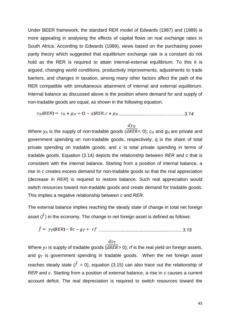
45
Under BEER framework, the standard RER model of Edwards (1987) and (1989) is
more appealing in analysing the effects of capital flows on real exchange rates in
South Africa. According to Edwards (1989), views based on the purchasing power
parity theory which suggested that equilibrium exchange rate is a constant do not
hold as the RER is required to attain internal-external equilibrium. To this it is
argued, changing world conditions, productivity improvements, adjustments to trade
barriers, and changes in taxation, among many other factors affect the path of the
RER compatible with simultaneous attainment of internal and external equilibrium.
Internal balance as discussed above is the position where demand for and supply of
non-tradable goods are equal, as shown in the following equation.
......................……………………3.14
Where yN is the supply of non-tradable goods ( < 0); cN and gN are private and
government spending on non-tradable goods, respectively; q is the share of total
private spending on tradable goods; and c is total private spending in terms of
tradable goods. Equation (3.14) depicts the relationship between RER and c that is
consistent with the internal balance. Starting from a position of internal balance, a
rise in c creates excess demand for non-tradable goods so that the real appreciation
(decrease in RER) is required to restore balance. Such real appreciation would
switch resources toward non-tradable goods and create demand for tradable goods.
This implies a negative relationship between c and RER.
The external balance implies reaching the steady state of change in total net foreign
asset ( ) in the economy. The change in net foreign asset is defined as follows:
……………......................................……. 3.15
Where yT is supply of tradable goods ( > 0); rf is the real yield on foreign assets,
and gT is government spending in tradable goods. When the net foreign asset
reaches steady state ( = 0), equation (3.15) can also trace out the relationship of
RER and c. Starting from a position of external balance, a rise in c causes a current
account deficit. The real depreciation is required to switch resources toward the

46
tradable sector and create demand for non-tradable goods to restore external
balance. This reveals a positive relationship between RER and c.
Solving equations (3.13) and (3.14) yields the determinants of RER as shown in
equation (3.15) below:
( )
Since f* is determined at the steady-state equilibrium, it is unobserved data. Under
the assumption of credit ceiling constraint, f* become exogenous and at the external
equilibrium, the negative value of rf* (-rf*) equals the country’s current account
balance net of interest transfer (Jongwanich, 2010). A widening current account
deficit implies that the country relies on higher net foreign capital inflows to maintain
external balance. The (equilibrium) RER must appreciate in order to restore
equilibrium. Capital flows and government spending are not the only fundamental
variables that could shift the internal and external balance and therefore affect the
RER.
In addition to capital flows, government spending on tradable and non-tradables
goods, equation 3.15 can be extended to reflect other variables that shift the internal
and external balance and hence affect the RER. Edwards (1989) presented a
theoretical way of analysing the way in which real exchange rates react to a number
of real disturbances that include changes in tariffs system, terms of trade (TOT)
shocks, and technological progress. A shift in a county’s trade toward greater
liberalisation leads to an increase in demand for tradable goods, with the RER
required to depreciate in order switch the demand from tradable to non-tradables
goods and then restore internal-external balance. In theory it is not clear how terms
of trade (ratio of export to import prices) impact RER, but if the income effect
associated with terms of trade deterioration dominates the substitution effect, a
worsening in TOT will result in RER depreciation. Technological progress variable is
based on Balassa (1964) reinterpretation of the PPP theory. A faster technological
progress is usually associated with stronger productivity in the tradables sector than
in the non-traded sector resulting in RER appreciation as prices of the non-tradables
tend to rise relative to prices of the tradables. It is necessary at this point to turn to
empirical studies, to assess the applicability of these different economic
fundamentals as determinants of RER.

47
From the three popular theoretical approaches of real exchange rate determination
discussed here, it suffice to say that in recent approaches (FEER and BEER) capital
flows are a significant component of the set of economic fundamentals of real
exchange rates. This is due to the approaches’ inclusion of the external balance,
which in essence implies reaching the steady state of change in total net foreign
asset in the economy.
3.2.3. The Fisher Effect (Interest Rate Factor)
Interest rate differentials play a role in determining the exchange rate as capital flows
in or out of a country. This is one of the international parity conditions. As more
capital flows to the country, the currency will appreciate, however, the Fisher
equation also only holds in the long run, (du Toit, 2005). Although the interest rate
plays a definite role, other factors like risk, news and expectations may overshadow
the day-to-day capital flows to and from a country. In recent years the flow of capital
in the global markets due to trade in financial assets has come to the point where
interest rates play a large role in determining where capital will tend to go. These
flows of capital determine the exchange rate in the short-medium term. However,
capital is a coward and will hit the road at the slightest sign of potential losses in the
current location or better prospects in another location. It is therefore not surprising
that exchange rates are volatile in response to new and unexpected news becoming
available in the market.
According to du Toit (2005), trade that results in the flow of capital across countries
will influence currency movements. This trade can be in the form of the traditional
goods and services, or in financial instruments between major market players.
Capital flows have been identified as a medium term determinant of exchange rate,
along with monetary and fiscal policy, and international parity conditions among
others. Figure 3.1 below identifies the different determinants of the exchange rate,
categorised under the time horizons that they are significant.

48
Figure 3.1 Exchange Rate Determinants
Source: Rosenberg (2003)
Since the main focus of this study is to assess the impact of capital flows in its
disaggregated form on real exchange rate, the discussion on this schematic diagram
had zeroed on capital flows (under medium-run determinants). Foreign demand for a
country’s currency will lead to an increase in the value of the domestic currency.
Capital flows can come from foreign direct investment (FDI), a flight to quality,
perceived strength, or the existence of investment opportunities.
3.2.3.1. The Mundell-Flemming model
In the Mundell-Flemming model, an expansionary fiscal policy typically helps raise
domestic interest rates and increases domestic economic activity Hinkle, &
Nsengiyumva, 1999). Increased domestic interest rates should result in an increase
capital inflow, which can either increase the currency’s value, at the same time
increased domestic economic activity can contribute to a deterioration of the trade
account, and/ or decrease the currency’s value. Figure 3.2 below illustrates how an
expansionary fiscal policy feeds into capital (in) flows, passing through to overall
balance of payments and ultimately the currency value.

49
Figure 3.2 Mundell-Flemming Model
Source: Rosenberg (2003)
From the analysis here, level of interest rates (or policies that lead to their increase)
determines the direction of the movement of capital across borders. Other factors will
further determine which type actually flows out or into the economy. Theoretically it is
clear that capital flows affect the exchange rates, however empirical analysis need to
be done and be assessed against the theory outlined in this section.
Neoclassical theory arguments are confirmed in Reinhardt, Ricci and Tressel (2010)
that less developed countries proved to experience net capital inflows and more
developed countries experienced net capital outflows, conditional of various
countries’ characteristics. Capital goes where the marginal return will be higher,
supported also by law of variable proportions. Net capital inflows to South Africa are
expected based on the classical theory assumptions. Firstly, South Africa has made
progress with regards to fundamentals that affect the production structure of the
economy, such as technological developments, factors of production, government
policies, and the institutional structure. Secondly international capital market
imperfections, such as sovereign risk and challenges of asymmetric information, are
not a major challenge for South Africa given its sophisticated financial markets.
Expected return on investment is high in many developing countries, and the high
level of uncertainty associated with those expected returns have been reviewed

50
downwards due to the high levels of defaults by developed countries- there has been
a swing in default risk between emerging economies and developed counterparts.
At some point in time, the different theories of exchange rate determination
discussed above, have shaped different studies with different conclusions reached.
To further argue on the role of different types of capital flows in determining real
exchange rates, there is need to critically review empirical literature to date so as to
guide the empirical analysis in this study.
3.3. Empirical Evidence
Since Salter’s seminal paper in 1959, it has been widely accepted that the real
exchange rates respond to capital flows. Over the past two to three decades
empirical investigations on impact of capital flows on real exchange rate have taken
center stage necessitated by currency crushes and financial crises that robed many
economies their celebrated growth paths. However, limited studies have been
conducted to determine the impact of capital flows on real exchange rate in South
Africa and other developing countries, let alone the impact of disaggregated capital
flows. Specifically, there are no studies that have analysed the impact of different
types of capital flows on the real exchange rate in the South African economy. The
existing empirical literature, disputes the appropriateness of the purchasing power
parity (PPP) as a model for the determination of the equilibrium real exchange rate,
because of the slow mean reversion of real exchange rates to a constant level (long
run equilibrium implied by the PPP assumption). As a result, there has been a shift
away from PPP-based model of the equilibrium real exchange rate to the
behavioural and fundamentals frameworks, such as those by Edwards (1987),
(1989) and Mtonga (2006), offered in the previous section. These observations will
influence the sections to follow in this study.
There are several ways of categorising empirical literature on the behaviour and
determinants of the real exchange rate, (Takaendesa, 2006). These include grouping
by the type of analysis employed, for example country-by-country analysis, cross-
section analysis and panel data analysis, and categorisation by countries studied,
such as studies of developed countries or developing countries. According to
Takaendesa, the latter categorisation allows sensitivity to structural differences

51
amongst these country groupings. The categorisation by countries studied will be
adopted for this study. It follows then, that this section is divided into empirical
evidence from developed countries, developing and other emerging economies, and
finally narrowed down to empirical literature from South Africa.
3.3.1. Evidence from Developed Economies
From developed economies the major studies are Brooks, Edison, Kumar and Sløk
(2004), Nilsson (2004), and Castilleja-Vargas (2009)
Brooks, et al (2004) explored the ability of portfolio and foreign direct investment
flows to track movements in the euro and the yen against the dollar. Net portfolio
flows from the euro area into US stocks (perhaps reflecting differences in expected
productivity growth) followed movements in the euro against the dollar closely. Net
FDI flows, which capture the burst in cross-border mergers and acquisition activity,
appeared less important in tracking movements in the euro-dollar rates, probably
because many mergers and acquisition transactions consist of share swaps. The
authors argued that movements in the yen versus the dollar remain more closely tied
to conventional variables such as the current account and interest differential. Large
inflows into the US equity markets and direct investment flows have financed the
current account deficit and allowed the dollar to remain strong. Capital inflows
therefore are not always bad. Conversely, large and initially unanticipated outflows
from the euro area appeared to account for a substantial part of its fall and persistent
weakness, (Brooks, et al., 2004). An analysis of bilateral exchange rates and current
account balances showed that the latter are generally not significant for explaining
exchange rate movements. On the other hand analysing the relationship between
exchange rates and portfolio flows suggested that in the second half of the 1990s, in
the case of the euro area, there was a strong relationship between exchange rate
movements and equity flows. An increase in equity flows to the USA was associated
with a clear depreciation of the euro (or synthetic euro prior to 1999) in relation to the
US dollar, added the authors.
Similarly, Nilsson (2004), examined the long-run relationship between the real
effective exchange rate and its fundamental determinants, and derives a real
effective equilibrium exchange rate for the Swedish krona. The relative effective
terms of trade, the relative effective price of tradables to non-tradables, and net

52
foreign debt as a share of GDP were considered as the fundamentals. The estimated
parameter of the net foreign debt ratio is -0.10, meaning an increase in net foreign
debt by 1 percent of GDP requires a 0.10 percent depreciation of the real exchange
rate to restore equilibrium. The adjustment coefficient in the net foreign debt ratio
equation, however, comes out to be negative and significant. Since the parameter of
the net foreign debt ratio in the co-integrating vector is negative as well, the equation
has a destabilising tendency in the system. This is clearly a desired property, as an
undervalued real exchange rate should tend to contribute to a decreasing net foreign
debt ratio and thereby cause the real exchange rate to become increasingly
undervalued. Even though this equation is destabilising, the overall system is stable
due to the relatively high speed of adjustment of the real exchange rate.
In Castilleja-Vargas (2009), the estimates showed no significant correlation between
net capital inflows and the real exchange rate with panel data of developed countries
using Fixed-Effects, the Arellano and Bond first difference and system GMM
estimators in its one-step modality (assuming homoskedastic errors).
3.3.2. Evidence from Emerging Market and Developing Economies
Studies on emerging markets (except South Africa) and developing economies
include those of Agenor et al. (1997), Dabos and Juan-Ramon (1998), Korsu and
Braima (2006), Feridun (2008), (Jaeger 2010), Jongwanich (2010), Ibarra (2011),
and, Combes et al (2011), among others.
In the context of an empirical model, Elbadawi and Soto (1994) examine the impact
of capital flows, among other fundamentals, on long-term exchange rates in Chile.
The real exchange rate and its fundamentals were found to be co-integrated during
1960-92. This co-integration allowed a reinterpretation of uni-equatorial estimates of
the equilibrium real exchange rate (ERER) to be consistent with long-run forward-
looking behavioural models. It also permits the estimation of an error-correction
model capable of disentangling short-run from long-run shocks in observed
movements of the ERER. This is a key technique given the non stationarity of most
economic time series. According to the authors, the non-stationary nature of the
fundamentals allows one to decompose innovations into permanent and transitory
components - to get an empirical measure of the sustainability of the fundamental
with which the ERER is determined. Generally the study found out that the estimate

53
of the co-integration of the ERER and its corresponding dynamic error-correction
specification corroborates the theoretical model and produces fairly consistent
results. The derived ERER index and the corresponding real exchange rate
misalignment (for given sustainable values of the fundamentals) successfully
reproduce the salient episodes in Chile's macroeconomic history. The study
disaggregated capital flows into four components: 1) short-term capital flows; 2)
long-term capital flows; 3) portfolio investment; and 4) foreign direct investment.
Short-term capital flows and portfolio investment were found to have no effect on the
ERER (although they can affect the real exchange rate in the short run). But long-
term capital inflows and foreign direct investment have a significant appreciating
effect on the ERER. To the extent that the then inflow of capital to Chile was
dominated by long-term capital flows that are judged to be sustainable, an important
part of the ensuing appreciation of the real exchange rate is consistent with
equilibrium behaviour - reducing the need for counterbalancing exchange rate on
macroeconomic policies.
Agenor et al. (1997) examined the relationship between the real exchange rate and
fiscal policy and capital inflows in Turkey using a VAR model. The study concluded
that positive shocks to government spending and capital inflows lead to an
appreciation of the real exchange rate.
On the other hand Dabos and Juan-Ramon (1998) estimated the long-run response
of the export (and true) real exchange rate to capital inflows in Mexico for the period
1970:1– 97:4, and for the sub-periods prior and after the trade liberalisation and
other structural reforms initiated in 1984 along the lines of Salter (1959) and
Rodriguez (1994). The authors also examined the short-term dynamic properties of
a system involving capital inflows, the external terms of trade, and the real exchange
rate and found that the system is a stable, true error correction model, and that
deviations from equilibrium due to exogenous shocks are corrected in about 14
quarters.
The empirical findings suggest that there exists a long-run relationship between the
ratio of capital inflows to GDP, the external terms of trade, and the export (and the
true) real exchange rate. Based on the estimated relationship for the sub-period of
greater openness (1984:2–97:4), a once and for all increase in the ratio of capital

54
inflow to GDP by one unit would, other things equal, lead to a long-run real
appreciation of the peso of about 21 percent (as defined by the export real exchange
rate) or about 42 percent (as defined by the true real exchange rate).
Dabos et al (1998) tested the Sjaastad and Manzur (1996) hypothesis that (because
protection reduces not only the volume of trade but also the margins of substitution
between traded and non-traded goods) capital movements have less impact on the
real exchange rate (thus, it exhibits less variability) when the economy is more open.
The findings failed to support the hypothesis. In fact, the long-run response of the
real exchange rate to capital movements was found to be greater in the second sub-
period when the economy was more open. In the same context, the authors also
conducted variance tests of the export real exchange rate and the ratio of capital
inflow to GDP and failed to reject the hypothesis of no difference between the
variances across sub-periods for these two variables at a unit percent significance
level. Openness (financial liberalisation) has been implied to have a role in
determining extent of the response of real exchange rate to capital movements in the
study by Dabos et al (1998).
Kim, S., Kim S.H. and Wang (2004) examined the macroeconomic effects of capital
account liberalisation in Korea. In their study simple data analysis suggested that
capital account liberalisation substantially changed the nature and composition of
capital flows. Based on the VAR model, the authors discovered the following: after
capital market liberalisation, capital flows become less driven by current account
imbalances and therefore become more autonomous; capital account liberalisation
significantly changes the effects of capital flows on macroeconomic variables; capital
account liberalisation is highly related to consumption and investment booms, and
subsequent appreciation of nominal and real exchange rates, which leads to the
current account worsening; and finally, there is strong evidence of sterilised foreign
exchange market intervention in response to capital inflows.
Indonesia’s financial sector liberalisation succeeded in strengthening the capacity of
the domestic financial system and promoting the rapid expansion of foreign capital
inflows for financing national development, argued Goeltom (2005). Contrary to that,
in the first half of the 1990s huge inflows of capital, much of which were short-term,
led to asset price bubbles in the property sector and superfluous credit expansion

55
that threatened financial system stability. According to the author, Indonesia became
an easy target for speculators because of weaknesses in the financial system, poor
corporate governance and heavy dependence on the external sector. As a result, the
economy plunged into a prolonged crisis. An open economy offers a means of
financing development beyond the capacity of domestic sources as globalisation is
an unstoppable phenomenon an economy must do what is necessary to profit from
such trend. Goeltom (2005), argued that the monitoring of foreign exchange flows
will not be aimed at imposing restrictions on capital flows, but instead, it is more for
statistical purposes in support of monetary policy and improved transparency, one of
the prerequisites for the creation of an efficient market.
Korsu and Braima (2006) based on the inter-temporal optimizing framework of
Edwards (1989) investigated the determinants of the real exchange rate for Sierra
Leone by controlling also for the effects of price changes, using annual aggregate
data from 1970 to 2005. Unit root and co-integration tests were carried out and an
error correction model of the actual real exchange rate model was estimated in the
context of Hendry’s general-to-specific modeling while the equilibrium real exchange
rate is estimated using the Johansen Maximum Likelihood procedure. The results of
the error correction model shows that increase in the price level, capital inflow,
capital accumulation and trade restrictions appreciate the actual real exchange rate
of Sierra Leone. Capital accumulation, increase in output, increase in government
expenditure and trade restrictions appreciate the equilibrium real exchange rate
Feridun (2008) investigated the determinants of two major currency crises of 1994
and 2000–2001 in Turkey. The results suggested that the currency crises in Turkey
are associated with capital reversals, or the “sudden stops” of capital inflows. This is
one of the dangers of allowing too much ‘hot’ money into the system. The author
argued that the results are supportive of the analysis of the Turkish monetary policy
by Balkan and Yeldan (2002), who explained that with the opening up of the Turkish
economy to the speculative foreign transactions, the Central Bank is bound to take a
passive role, and the domestic economy is trapped into the vicious cycle of high real
interest rates together with an overvalued domestic currency. Strong evidence
emerged that increases in US interest rates lead to an increase in the likelihood of a
currency crisis in Turkey, and also an increase in the real interest rate differential

56
between the three-month US deposit rate and the three-month Turkey deposit rate
increase the likelihood of a currency crisis in Turkey asserted Feridun, (2008). The
findings reveal that increased devaluation expectations caused by higher US interest
rates lead to a self-fulfilling speculative attack on the Turkish lira. To the author, the
finding is not surprising as a large percentage of the capitalisation of the Istanbul
Stock Exchange is owned by foreign investors, who can withdraw their funds at any
time if they that find investing elsewhere are more profitable. Risk aversion inherent
with investors has created instabilities within many economies and the endangering
fact is that, loss of appetite on assets from a particular country has a contagion effect
to the assets of other countries of the same class (for example emerging markets).
According to Castilleja-Vargas (2009), unlike developed countries, changes in net
capital flows are significantly positively correlated with real exchange rate
movements in emerging markets.
For Mexico, Ibarra (2011) studied the effect of the different types of capital flows on
the real exchange rate. Long-run real exchange rate equations were estimated
following the bounds testing approach of Pesaran et al (2001). The methodology
used control set of variables (fundamentals), comprising the ratio of industrial
production between Mexico and the US, the ratio of the share of government
consumption in GDP between the same countries, and the international price of oil
(as an indicator of Mexico’s commodity terms of trade). The fundamentals are the
immediate determinants of real exchange rate which, and the expected future
evolution, will detect the path of the exchange rate of an economy. The author
argued that, foreign capital inflows allow a country to run current account deficits and
thus attain higher investment levels without having to sacrifice consumption. Any
economy would prefer this benefit, let alone emerging market economies with limited
capital resources. However, Ibarra (2011) claims that the inflows tend to appreciate
the recipient country’s currency in real terms and reduce profitability in the tradables
sector, resulting in current account deficits that have as counterpart booming
consumption but depressed investment levels. Resultantly, the study added; the
potentially positive influence of capital flows on economic growth will be undermined.
The major finding of the paper is that not only portfolio investment but also FDI can
strongly appreciate the recipient country’s currency. This phenomenon, however

57
cannot be easily generalised as country characteristics play a significant role, even
among those economies with similar growth prospects.
The level of capital flows to the BRICs (Brazil, Russia, India and China), a group of
emerging market economies- differs markedly, with Brazil experiencing the highest
level of inflows during 2009-10 due to its more open capital markets (compared to
China and India), perceived improvement in post-crisis growth and/or lower
“leverage” (compared to Russia) and very high interest rates, noted (Jaeger 2010).
South Africa’s level of inflows recorded sharp increase during 2009-10, see Creamer
(February 2011), giving an unprecedented upward pressure on the Rand. Jaeger
(2010) further argued that, the degree to which countries are struggling with capital
inflows differs significantly, as they do with respect to their policy responses in terms
of currency appreciation, reserve accumulation and capital controls. It is therefore
imperative to understand the actual impact of capital flows on exchange rate for a
particular country in order to respond correctly. According to Bhinda, Leape, Martin,
Griffith-Jones, et al (1999), following heavy capital outflows in early 1994, South
Africa experienced a surge in capital inflows after the successful democratic
elections in April 1994.
According to the Deutsche Bank Research (February, 2011) BRICs currencies have
been appreciating in real terms, within the last two years (2009-2010), the Russian
rubble and Indian rupee have appreciated by more than 10% in real effective terms.
The Chinese Yuan had barely moved and the Brazilian real had strengthened by
40%, albeit from depressed post-crisis levels. The Brazilian real had also
appreciated the most in nominal terms. The report noted that it is not surprising
therefore that the Brazilian authorities should have taken the most aggressive
measures aimed at slowing capital inflows. The appreciations of the respective
currencies are linked to the increase in capital inflows. The capital influx worries can
also be deduced from the joint statement by BRICS officials (at the first BRIC[S]
Summit including South Africa on 14 April 2011: Sanya, China) as they warned that
developing countries face risks from capital inflows caused by loose monetary
policies in developed nations (Kolyandr and Fletcher, 2011). South Africa has a lot to
learn from fellow emerging markets, in terms of dealing with exchange rate pressure
mainly from the increased influx of capital flows.

58
Jongwanich (2010) noted that, one of the unfavourable side effects of “too much”
capital flows is (real) exchange rate appreciation, or loss of a country’s
competitiveness, which could unfavourably distress tradable production and export
sectors. Jongwanich further argued that RER appreciation occurs regardless of the
exchange rate regime implemented in a country; with a flexible exchange rate
regime, (real) currency appreciation occurring due to the appreciation of the nominal
exchange rate while under a fixed exchange rate regime, the appreciation comes
mainly through a rise of non-tradable prices. With globalisation, any country would
want to improve its competitiveness position or at least to remain competitive so as
to reap the benefits that come with such an economic setup. This brings out the
importance of real exchange rate in an economy, more specifically emerging open
market economy like South Africa. Real exchange rate is a key policy variable in
South Africa’s open economy, Aron, Elbadawi and Kahn (1997). Jongwanich (2010)
paper tried to answer the following questions,
how far the real exchange rate can be adjusted in response to capital flows
whether the composition of capital flows matters in determining the
movements of the (real) exchange rate
whether capital inflows and outflows impact in various ways on RERs;
by using a dynamic panel data model for emerging Asian economies to examine the
relationship between capital flows and RER. The author estimated RER as a function
of government spending (GSPEND), net flows of foreign direct investment (FDI), net
flows of portfolio investment (PORT), net flows of other investment flows (bank
loans) (OTHIN), difference in the rate of productivity growth in tradable-good
production of a country i at time t compared to that of the main trading partner
countries (PRODi ,t), terms of trade (TOT) and trade openness (OPEN). This study
will try to answer the last two questions with respect to South Africa.
All capital flow elements (FDI, PORT, and OTHIN) were further divided into inflows
and outflows to form a second model, and lastly dummy variables were introduced to
have a third model in Jongwanich (2010). The distinction among capital flows with
regards to composition and directional flow is very crucial and can be highly
informative to policymakers. Few studies have disaggregated capital flows according
to composition (type), with particular reference to South Africa. Jongwanich pointed

59
out that, there has been no systematic analysis that studies how different types of
capital flows impact (real) exchange rates. This paper will take note of this and will
disaggregate capital flows according to composition in South Africa, an economy that
had witnessed a great volatility in its currency.
Bakardzhieval, Naceur, and Kamar (2010) asserted that attracting capital and foreign
exchange flows is crucial for developing countries. The authors noted that these
flows could lead to real exchange rate appreciation and may thus have detrimental
effects on competitiveness, jeopardizing exports and growth. The study investigates
the dilemma by comparing the impact of six types of capital and foreign exchange
flows on real exchange rate behavior in a sample of 57 developing countries
covering Africa, Europe, Asia, Latin America, and the Middle East. The study’s
results reveal that portfolio investments, foreign borrowing, aid, and income lead to
real exchange rate appreciation, while remittances have disparate effects across
regions. Foreign direct investments have no effect on the real exchange rate,
contributing to resolve the above dilemma. As a panel data analysis the study used
Generalized Method of Moments (GMM) estimator, which corrects for both of these
biases and takes into account the dynamics of real exchange rates. This estimation
technique is not possible in this study since the data is time series and not panel
data.
Combes et al (2011) distinguished between public capital flows (official loans, debt
interest and official transfers) and private capital flows (private transfers, FDI, FPI,
and commercial bank loans). The ‘Other’ capital flows in Jongwanich (2010) as
discussed above were further disaggregated into bank loans and private transfers.
The authors noted that, the spectacular rise in private flows in the past years have
been driven by FDI and current private transfers mainly remittances, although
appreciating the significance of commercial bank loans. Using a sample of 42
developing countries for 1980-2006, Combes et al applied a pooled mean group
estimation technique that allowed short-run heterogeneity while imposing long-run
homogeneity on the real exchange rate determination across countries. They found
aggregated capital inflows as well as public and private flows to be causing real
exchange rate appreciation. Using a de facto measure of exchange rate flexibility,
they found that exchange rate flexibility helps dampen real appreciation due to

60
capital inflows. It is also crucial to test the significance of exchange rate flexibility on
mitigating currency pressures due to surges in capital flows in South Africa.
Contrary to the majority of studies Sy and Tabarraei (2010) concluded that real
fundamentals are the main driving forces of real exchange rate movements in less
developed countries (LDCs) not capital inflows. The study covered the period 1970
through to 2004. The Balassa-Samuelson effect in their study accounts for 57% of
the RER variations while capital inflows account only for 19% of RER variations. The
Dutch Disease theory is not rejected but its effect on RER movements in LDCs is
weak. The study tested the link between capital inflows and real exchange rate
movements in LDCs theoretically and empirically. Capital inflows in their study were
suggested to be oil revenues, foreign aid, remittances or FDI. Overall their study
concluded that capital inflows affect the real exchange rate in the short run and
mainly the productivity in the long run.
Okonjo-Iweala (2011), (managing director at the World bank), as quoted by Gray
(2011) argued that: though investment funds had flowed into emerging markets and
some frontier markets in recent years, many African countries enjoying growth are
struggling to attract the attention of a broad range of investors (these bring different
forms of capital). Okonjo-Iweala (2011), advocates for more foreign investors, in
other words an encouragement of capital inflows in order to boost economic growth
in Africa. These arguments however seem to be disconnected from real-world
experiences, as an influx of the capital tends to pose great policy dilemma to the
same policymakers, Singh (2003). Policymakers have been, of recent, left in the
doldrums with the effects of surges in capital inflows on the domestic currency; see
van der Merwe (2003). One such effect is the pressure on the domestic currency, an
appreciation of the currency when inflows grow.
3.3.3. Evidence from South Arica
Studies modelling capital flows and real exchange rates in South Africa are skimpy
considering the role capital flows play in determining exchange rates, and those
disaggregating capital flows in the three official categories are non-existent. The
studies analysing capital flows and exchange rates in South Africa include Bhinda, et
al, et al (1999), Wesso (2001), Mohamed (2006), Aron, Leape and Thomas (2010),
among others.

61
Changes in amount and direction of capital flows will result in gross negative
repercussion on the economy as a whole. Such changes in external capital flows can
have strong effects on inflation and real economic activity through their effect on the
[real] exchange rate and the cost of capital; in some circumstances countries have
experienced them as a ‘sudden stop’ and wide-ranging crisis, Harris (Undated).
Policy dilemma will be experienced as there will be need for trade-offs since
addressing one challenge may worsen the other. Intervention in the foreign
exchange market in response to capital flows enables authorities to influence the
stability of the real exchange rate, however, attaching a single policy instrument to
multiple objectives inevitably leads to conflicts, forcing authorities to make trade-offs,
Bhinda, et al, (1999).
Foreign capital is crucial for supporting economic growth in any economy, South
Africa not an exception. Policymakers therefore formulate policies that attract
investors in order to contribute to the domestic economy’s growth. Wesso (2001)
argued that South Africa needs foreign capital in order to support economic growth in
the country with tax reforms, fiscal discipline and the gradual liberalisation of
exchange control [in the past] all aimed at increasing its attractiveness as a
destination for foreign investment. The SARB has classified capital flows into: foreign
direct investment, which involves investment in a firm where foreign investors have
at least 10 per cent of the voting rights; foreign portfolio investment which includes
the purchase and sale of bonds and equities listed on international and domestic
capital markets; and other foreign investment which consists of foreign loans and
deposits between banks, companies and governments. This classification will be
adopted for the purpose of this study, as also data is available for al the categories.
Simwaka (2004) analysed the contributions of economic fundamentals as
technological progress, degree of openness, government consumption, nominal
devaluation, international capital flows, excess domestic credit to the determination
of real effective exchange rate (REER) in Malawi (1980-1999) and South Africa
(1987-1999). The coefficient on capital flows had different signs, positive for Malawi
and negative for South Africa. Simwaka concluded that, the effect of capital flows on
REER depends on whether the capital flows are spent on either traded or non-traded
sector; therefore differing relationships are expected across countries.

62
Mohamed (2006) examined the effects of more domestic liquidity as a result of the
large net capital inflows and argued that surges in inflows are of concern because
they increase potential for financial risk and instability in the economy. This is one of
the few empirical analyses that modelled capital flows, especially looking beyond
FDI. The research revealed that the surges in capital flows have not been well
absorbed into the South African economy; apparently there was little or no
investment except consumption and asset price bubbles that increased financial
fragility. This strengthens the doubt about the economic benefits of large capital
flows despite arguments by Aron, Leape and Thomas (2010) that foreign capital
inflows play a critical role in sustaining higher levels of investment and growth in
South Africa given the persistently low national savings rate and consequent savings
deficit. All the same no reference to the impact of these capital inflows on
macroeconomic variables such as exchange rate had been made.
Real exchange rate determinants according to Mtonga (2006), includes: domestic
supply-supply side factors, stance of fiscal policy, factors related to changes in the
country’s international economic environment (including flow of international capital
and transfers), and stance of trade and commercial policy. All these identified, are
crucial economic fundamentals with regard to real exchange rate movements.
One of the main mandates of central banks is maintaining financial stability which
entails ensuring a stable currency relative to those of other economies, especially
major trading partners. Siourounis (2003) suggested that, the reason of investigating
the empirical relationship between capital flows and exchange rates is motivated by
modern international finance theory which asserts that currencies are as much
influenced by capital flows as by account balances and long-term interest rates.
3.3.4. Hypothesized link between foreign exchange markets and the capital account
Agenor and Hoffmaister (1998) put forward two factors that determine the evolution
of real exchange rate response to surges in capital flows. The first being the
macroeconomic response, the second and of interest to this study is the composition
of the flows and their effects on the composition of aggregate demand. The
abundance of private capital inflows confronted many Asian and Latin American

63
authorities with a transfer problem, (Reisen, 1998). This had proved to be a
challenge beyond Latin America, but inherent with most developing and emerging
market economies (DEM). The authorities are left with no option but to consider
whether to control the flow of capitals (BRICS, 2011) or how much to accept/ resist,
based expectantly on the different types of capital flows. FDI component of capital
flows is well known for its contribution to the expansion of production capacity
through bringing or enabling acquisition of technology and expertise. On the other
hand, FPI, bank loans and remittances among others, often sustain consumption
thereby shifting the aggregate demand only. Controlling capital flows in general may
not be justifiable without understanding their behaviours in disaggregated terms.
It has been noted above that, the composition of the capital flows and their effects on
the composition of aggregate demand determine how they impact foreign exchange
rate. It can now be hypothesised that an exchange rate can come under pressure
from surges in capital inflows. According to SARB, (2010), it only requires net capital
inflows to fall to levels below the prevailing deficits on the current account for the
exchange rate to start coming under pressure. The portrayed linkage implies the
significance of capital inflows in determining the path of the exchange rate;
especially as it cannot be expected for South Africa to experience steady net capital
inflows.
A major fall of the Rand’s value during 2007-08 could be ascribed to innumerable
factors that do not allow a cut in the flow of capital from South Africa. One of the
factors, according to SARB (2011), is the disinvesting by foreigners from SA equity
markets, resulting in JSE all-share index falling by about 36% from November 2007
to October 2008. On the other hand, the strength of the Rand in 2009 is ascribed to
the return of international investors to emerging market countries, the weakness of
the US dollar and the steady ascendants of commodity prices during that period.
3.4. Assessment of Literature
The behavioural exchange rate determination approach is going to be adopted in this
study, ensuring internal and external sector equilibrium. This approach allows the
identification of fundamental variables that impact the real exchange rate. It is
necessary to hypothesise a high volume of capital inflows to South Africa due to the
sophisticated financial market, despite disagreement on the real effects of such on

64
major economic variables. This then rules out the Lucas paradox in the South
African context, as, though a developing country; there are more inflows than
outflow. The neoclassical theory is therefore likely to hold. There is limited empirical
work for South Africa along this topic, more especially ones modelling disaggregated
capital flows. This study will contribute immensely to the literature. There is evidence
that, even if economies can be classified in the same group, for example BRIC[S],
their experience with capital flows differs markedly, therefore encouraging us to
focus on South Africa and have an in-depth analysis rather than generalisation.
Some key variables worth considering are the conventional set of fundamentals
suggested by most researches in explaining movements in real exchange rate.
These variables include productivity gap/ technological progress; terms of trade;
trade policy (openness), and government spending; see Simwaka (2004),
Jongwanich (2010), and Combes et al (2011). The variables are worth considering in
this study as they help specify our model.
From the studies reviewed, it is apparent that the common model is multivariate
encouraging the use of the vector-autoregressive (VAR) framework in conducting
empirical analysis.

65
CHAPTER 4: RESEARCH METHODOLOGY
4.1. Introduction
This chapter describes the analytical framework that is used in this study based on
the literature reviewed in Chapter 3. The main drive of this study was to assess the
impact of changes in different forms of capital flows on the real exchange rates in
South Africa. The real exchange rate empirical determination follows the internal-
external balance approach taking into account the economic fundamentals that are
central to real exchange rate movements as espoused in the preceding chapter on
literature review.
The chapter is split into the following major sub-sections: 4.2 Specifies the model;
4.3 spells out the data definition and the sources; 4.4 presents the methods of data
analysis and estimation techniques, while section 4.5 concludes and summarises the
chapter.
4.2. Model Specification
The general form real exchange rate model used in this study is based on works of
Elbadawi and Soto (1994), Edwards (1998), and Jongwanich (2010), with some
modifications. The theoretical underpinning of this empirical approach is based on
the internal-external balance framework of exchange rate determination. The
empirical approach takes the form:
................................................4.1
Where:
REERt = Real Effective Exchange Rate at time t
GSPENDt = government spending at time t
Kt = capital flows at time t
TOTt = terms of trade at time t
OPENt = trade openness at time t
TPt=technical progress measured by the industrial production index
EMPt = the measure for the flexibility of exchange rate policy in time t
The main variable of concern here is the Kt (total capital flows). There is great reason
to hypothesise a measurable influx of foreign investments to emerging markets. This

66
is supported by higher emerging market (EM) and lower developed market (DM)
creditworthiness which appears to persist. The swing in creditworthiness has been
behind the greater “calculated” asset allocation, especially in the form of portfolio and
short term investments, to EM by DM institutional investors, (Mallick and Sousa,
2009). This entails that, the effects of different forms (FDI; FPI; foreign bank loans
and remittances (OTHER foreign investments)) of foreign capital on real exchange
rates are a force worth to reckon. Due to this observation, and supported by
literature reviewed in preceding chapter, the Kt variable will be disaggregated into:
foreign direct investment (FDIt), foreign portfolio investment (FPIt), and other
investments (OTHINt).
There is no consensus on the influence exchange rate policy has in relation to the
impact of capital flows on real exchange rate. To assess the effectiveness of
exchange rate policy as a hedge against real appreciation due to capital inflows, an
exchange rate flexibility variable and its cross-term (with capital inflows variable) will
be added. The exchange market pressure (EMP) will be the proxy for exchange rate
flexibility. The degree of EMP is derived from the relationship between nominal
exchange rate and relative foreign reserves, Combes et al (2010), as:
EMP = %Δet -%Δft
Where %Δet is the variation of the nominal exchange rate (Δet) in year t expressed
as a percentage and %Δft is the percentage change in foreign reserves during year t.
The disaggregated linear model will take the form:
..….…..................... 4.2
Kt in equation 4.1 is disaggregated here into: FDI, FPI and OTHIN. Since we want to
measure the impact of different forms of capital flows on the real exchange rates, the
coefficients of main focus becomes β1, β2, and β3. The estimates of these
coefficients will be compared in terms of significance and impact exerted on real
exchange rate in order to determine which form is most influential. To ascertain the
influence the exchange rate policy has in relation to the impact of capital flows on
real exchange rate, coefficient α5 will be analysed.

67
4.3. Data Sources and Definition of Variables
This study employs data set on variables consisting of quarterly observations from
the first quarter of 1990 to the fourth quarter of 2010. The period of study is
motivated by the need to analyse the impact of capital flows on real exchange rate in
a period of new government and a set of economic reforms. The new government
started in 1994, however 1990 is chosen because of the processes pre 1994 election
which saw the removal of sanctions and other restrictions on South Africa. These
policies influenced the repositioning of South Africa into the world.
The data was obtained from South African Reserve Bank online statistical query,
International Monetary Fund (IMF’s) International Financial Statistics online
database, and World Bank Development Indicators among other sources. The
variables to be employed for the purposes of meeting the stated objectives ought to
be defined and a priori relationships highlighted.
4.3.1. Real Effective Exchange Rate
The CPI-based real effective exchange rate index for the Rand, provided by SARB
as average value of bilateral exchange rates for the period with respect to 15 trading
partners , weighted by volume of trade in manufactured goods between South Africa
and these countries was used. The real effective exchange rate of the rand is
measured in foreign currency terms (index, 2000=100), thus an increase in this
variable indicates an appreciation of the rand. The current weighting structure of the
index as described on SARB has been presented in Chapter 2 Table 2.1.
4.3.2. Government spending
This measures the fiscal position in the economy. Fiscal policy portrays an
ambiguous effect on REER as the direction of its quantitative influence depends on
the sectoral composition of the change in government expenditure, (Mtonga, 2006).
From literature, government spending on tradable and non-tradable sectors affect
the REER in a different direction. When government increase its spending on
tradable goods, the resulting effect would be an increase in import consumption,
raising demand for tradable goods and therefore bringing about a trade deficit. A
depreciation of the Rand would be required in order to restore external equilibrium.
On the other hand, when the increased spending is on non-tradable goods, this will

68
create an excess demand in the non-tradable goods market with an increase in the
relative price of non-traded goods required to maintain goods market equilibrium.
This therefore results in an appreciating real exchange rate. It seems to be
appropriate to include both expenditures in the REER function; unfortunately there is
no data available in such a disaggregated manner. GSPEND, the ratio of
government consumption spending to GDP expressed as percentage is an
acceptable proxy for the fiscal position. However, since government expenditure is
relatively more intensive in non-tradable goods sector, thus a negative relationship
between GSPEND and REER was expected. The source of the data for this
measure was the SARB.
4.3.3. Capital flows
The SARB classifies capital flows into:
a. foreign direct investment (FDI), which involves investment in a firm where
foreign investors have at least 10 per cent of the voting rights;
b. foreign portfolio investment (FPI) which includes the purchase and sale of
bonds and equities listed on international and domestic capital markets; and
c. Other foreign investment which consists of foreign loans and deposits
between banks, companies and governments
This classification was adopted for the purpose of this study, as also data was
available on SARB website for all the three categories. FDI, FPI and OTHIN
variables were expected to have a negative relationship with REER, implying a rise
in any of these result in REER appreciation (lower REER).
4.3.4. Productivity gap/ technical progress
This variable captures the potential Balassa-Samuelson effect. The differences in the
rate of productivity growth in tradable-good production of a country compared to that
of the main trading partner countries are a potential factor that affects the REER. It
is defined as a country’s GDP per capita relative to the weighted average GDP per
capita of its trading partners. The weights of the trading partners are similar to those
used in constructing REER. The assumption is that, productivity grows faster in
tradable than in non-tradable sectors. No source of data is available for this variable.
In empirical literature, however, the variable is usually proxied. We measured this

69
variable by relative real GDP per capita, which measures labour productivity as real
GDP divided by total population. The data source was the SARB. TP was expected
to have a positive relationship with REER.
4.3.5. Terms of trade
This is defined as the ratio of the world price of a country’s exports to the world price
of imports. The ratio captures the exogenous changes in world prices that will affect
the REER. This ratio captures factors related to changes in the economy’s
international economic environment. For South Africa, it either includes or excludes
gold exports/imports, and data source is the SARB. The effects of TOT cannot be
determined a priori; the empirical evidence, however, shows that improved TOT tend
to lead to REER appreciation. Mundell (1997) stated that there is no systematic
theoretic sign of the relationship between TOT and REER. TOT can worsen
(improve) because of increases (decreases) in the price of imports or decreases
(increases) in the price of exports. An improvement in a country’s TOT refers to an
increase in the price of its exportable goods relative to importable goods, and thus is
expected to appreciate the real exchange rate. According to Mtonga (2006),
increases in the price of exports allow growth of the export sector output, and thus
gives rise to excess supply of exportable goods and a trade surplus. This increase in
export sector output would allow an increase in the real wage in the traded goods
sector relative to that of the non-traded goods sector. As a result of this, a
redistribution of labour from the non-traded to the traded goods sector would be
expected. At the same time, output of non-traded goods would be expected to
contract, thereby creating excess demand in the non-traded goods market, and thus
a higher relative price. Both the improvement of the trade balance and the rise in the
price on non-tradable goods require an appreciation of the real exchange rate if
equilibrium is to be maintained.
4.3.6. Trade policy (trade openness)
This is defined as the ratio of the sum of imports and exports of goods and services
to GDP. It measures the commercial policy of the economy, how liberalised is the
economy. The ratio represents the trade policies as it is affected by factors such as
tariffs, quotas and subsidies that influence trade. The data source for imports,

70
exports and GDP is the SARB. The degree of liberalisation (OPEN) is expected to
have a positive relationship with REER as trade liberalisation works by channeling
resources from the tradable sector into the non-tradable sector. Trade openness
affects prices of non-tradables through income and substitution effects. A lower
openness level (restrictions on trade) has a negative effect on the prices of tradables
through income effect and a positive effect through substation effect. Trade
openness impact on the real exchange rate is mixed in the literature. Egert (2003)
drew up an overview of the real exchange rate determinants from empirical studies
and their coefficients’ expected sign. The expected sign depends on the
consideration at hand: considering openness as an indicator of trade liberalization,
an improvement in openness should lead to a depreciation of the real exchange rate.
On the other hand, it can be argued that supply capacity can be improved by
openness and this leads to an improvement in the trade balance and an appreciation
of the exchange rate.
4.3.7. Exchange rate market pressure
The argument by other researchers that the exchange rate regime has an influence
on how capital flows impact the real exchange rates necessitated the inclusion on
this variable. The EMP will be used to proxy, degree of exchange policy flexibility.
There are different measures of EMP which include: making use of the dummy
variable, de-jure and de-facto measures. For the purposes of this study the degree of
EMP is derived from the relationship between nominal exchange rate and relative
foreign reserves. The sign of the coefficient of EMP cross term with Kt variable is not
certain.
4.4. Data Analysis/ Estimation Techniques
The above specified model (equation 4.2) is subjected to a number of econometric
tests. Several techniques are available for parameter estimation, ranging from
classical regression methods to co-integration based techniques.
The classical regression methods are based on the assumption that all the variables
to be included in a regression are stationary (integrated of order zero), [I (0)], but
most economic series are not. Therefore estimations based on this technique will be

71
spurious. A preferred approach would be to successively difference the variables
until stationary is achieved, (Asteriou and Hall, 2007), but this throws away useful
long run information that may be in the data. This problem can be resolved by the
new generation of models based on co-integration and error correction modeling.
Unit root or stationarity tests will be done on all the series before proceeding with the
tests for co-integration and estimation of parameters. Both formal and informal unit
root testing methods were considered, and the one best suiting our model is chosen,
allowing for robustness checks. There are also several co-integration based
methods, those based on univariate versus those based on multivariate models.
Since the model used in this study is multivariate, there is a likelihood of having more
than one co-integrating vectors; therefore our selection was from those techniques
based on multiple equation regression.
4.4.1 Testing for stationarity/ Unit-root
The tests are meant to investigate if the series are stationary. Stationary is a key
concept underlying time series processes. According to Asteriou and Hall, (2007) a
time series is covariance stationary when it has the following three characteristics:
i. Exhibits mean reversion in that it fluctuates around a constant long-run mean;
ii. Has a finite variance that is time-invariant; and
iii. Has a theoretical correlogram that diminishes as the lag length increases.
Analysing non-stationary series has a general problem of the usual standard tests of
significance being invalid. Informal tests consisting of graphical analysis and
Correlogram (auto-correlation function) were performed to visually inspect the
behaviour of the variables under consideration.
4.4.1.1. Informal Unit Root Tests
4.4.1.1.1. Graphical displays
A popular informal test for stationarity is the graphical analysis of the series. This is a
visual plot of the series which is an important step in the analysis of time series
before pursuing any formal tests. This preliminary examination of the data (eye

72
balling) is important as it allows the detection of any data capturing errors, and
structural breaks and gives an idea of the trends and stationarity of the data set.
4.4.1.1.2. Correlograms and Q-statistics
Secondly, for informal tests, an inspection of correlograms (autocorrelation of
residual functions) is carried out. This allows examination of seasonal patterns of
time series. In essence, the correlograms displays graphically and numerically the
autocorrelation function (ACF), that is, serial correlation coefficients (and their
standard errors) for consecutive lags in a specified range of lags. Usually ranges of
two standard errors for each lag are marked in correlograms but normally the size of
auto correlation is of more interest than its reliability because of greater interest are
very strong and highly significant autocorrelations, (Gujarati, 2004).
There is serial correlation, that is, autocorrelation, when either the dependent
variable or the residual show correlation with its values in pasts periods. This is a
problem because standard errors are not consistent, affecting statistical inferences.
If there is no serial correlation in the residuals, the autocorrelations and partial
autocorrelations at all lags should be nearly zero, and all Q-statistics should be
insignificant with large p-values. A common finding in time series regressions is that
the residuals are correlated with their own lagged values. This serial correlation
violates the standard assumption of regression theory that disturbances are not
correlated with other disturbances, (QMS, 2009).
In the case of non-stationary processes, the theoretical autocorrelation coefficients
are not defined but one may be able to obtain an expression for E (r k), the expected
value of the sample autocorrelation coefficients. For long time series, these
coefficients decline slowly. Hence in time series analysis we can make an initial
judgment as to whether a time series is non-stationary or not by computing its
sample correlogram and seeing how quickly the coefficients decline. We turn to this
and the analysis of correlograms is subdivided into two analyses as follows:
4.4.1.1.3. Autocorrelations (AC)
The dotted lines in the plots of the autocorrelations are the approximate two standard
error bounds. If the autocorrelation is within these bounds, it is not significantly
different from zero at (approximately) the 5% significance level.

73
4.4.1.1.3.1. Partial Autocorrelations (PAC)
This is a partial correlation since it measures the correlation of Y values that are k
periods apart after removing the correlation from the intervening lags. If the pattern
of autocorrelation is one that can be captured by an auto regression of order less
than k, then the partial autocorrelation at lag k will be close to zero. Again, if the
partial autocorrelation is within these bounds, it is not significantly different from zero
at (approximately) the 5% significance level.
To consider whether a correlation coefficient of ACF is significant or not we judged
by its standard error. Bartlett (1950) has shown that if a time series is purely
Random, that is, it exhibits white noise the sample autocorrelation coefficients are
normally distributed with zero mean and variance equal to one over the sample size.
A non-stationary time series might need to be differenced more that once before it
becomes stationary, and if the series becomes stationary after d numbers of
differences is said to be integrated of order d.
According to Asteriou and Hall, (2007), most macroeconomic time series are trended
and therefore in most cases are non-stationary. As is with most economic and
financial series, the series in this study are not expected to be integrated of order
zero [I (0)], therefore allowing us to make use of co-integrating techniques.
4.4.1.2. Formal Unit Root tests
In simple terms, testing for unit roots is testing for the order of integration of a series.
Dickey and Fuller (1979, 1981) devised the procedure to formally tests for non-
stationarity arguing that testing for non-stationarity is equivalent to testing the
existence of a unit root. This is based on the assumption that is white noise
process from:
- = - + ………………………………………………………….……4.3
And
=
is stationary, thus differencing we obtained stationarity. Unfortunately the error
term ( ) is unlikely to be white noise, Dickey and Fuller extended their test
procedure providing an augmented version which includes extra lagged terms of the

74
dependent variable in order to eliminate autocorrelation. Hence, the augmented
Dickey-Fuller (ADF) test for unit roots which was employed in this study.
Dickey–Fuller tests are supported by the distribution theory based on the assumption
that the error terms are statistically independent and have a constant variance,
(Asteriou & Hall, 2007). This means effort should be made to ensure that error terms
are uncorrelated and that they really have a constant variance when using the ADF
methodology. Philips and Perron (1988) developed a simplified version of ADF test
procedure that makes mild assumptions concerning the distribution of errors, the PP
test. Strictly speaking, the PP test does not refute the ADF test but presents just
modifications of the ADF t statistics that take into account the less restrictive nature
of the error process. For this reason, the two tests were employed in this study for
robustness check purposes and they are discussed fully below.
4.4.1.1. Augmented Dickey Fuller (ADF)
Brooks (2004) asserted that the ADF test is more preferred to the DF test since the
later has critical values that are greater in absolute terms and may sometimes lead
to a rejection of a correct null hypothesis. The process involves estimating the
following equation:
= ∑ ........................................................................... 4.4
The lags of absorb any dynamic structure that may be present in the dependent
variable to ensure that εt is not auto correlated (Brooks, 2004). This test estimates
three models for each variable that is either with;
a. no constant and no trend;
b. constant and no trend; or
c. both constant and trend
The difference concerns the presence of deterministic elements (constant and
trend), and unless the actual data generating process is known, there is a question
concerning whether it is appropriate to estimate under assumption a, b or c,
(Asteriou and Hall, 2007).
Gujarati (2003) points out that the rationale behind introducing lags is to include
enough terms so that the error term is serially uncorrelated. With ADF, having too

75
few number of lags will not eliminate all of the autocorrelation while using too many
will increase the coefficient standard errors. The latter take place as an increase in
the number of parameters to estimate consumes the degrees of freedom. As a
result, Gujarati argues that the power of the test will be reduced, in the end, for
stationary process the null hypothesis of a unit root will less likely be rejected than
would have been the case otherwise.
4.4.1.2. Phillips-Perron (PP)
For robustness and to ensure accuracy of the unit root results, a second unit root
test by Phillips and Perron (1988) is used. The method employs a nonparametric
approach to control serial correlation in the error term. The test regression is the AR
(1) process:
....................................................................................... 4.5
The PP test makes a correction to the t-statistic of the coefficient from the AR(1)
regression to account for the serial correlation in whilst the ADF test corrects for
higher order serial correlation by adding lagged differenced terms on the right hand
side (Brooks, 2008). The PP test has been widely used in the empirical analysis
since it can be argued that both DF and ADF tests do not consider the cases of
heteroskedasticity and non-normality frequently revealed in raw data of economic
time series variables.
The advantages of the PP tests over the ADF tests include: the PP tests are robust
to general forms of heteroskedasticity in the error term( ), and the user does not
have to specify a lag length for the test regression. The Phillips-Perron (PP) unit root
tests differ from the ADF tests mainly in how they deal with serial correlation and
heteroskedasticity in the errors. The PP method estimates the non-augmented
Dickey-Fuller test equation and corrects for any serial correlation and
heteroskedasticity in the errors ( ) of the test regression by directly modifying the -
ratio of the coefficient, (Asteriou and Hall, 2007). The asymptotic distribution of the
PP modified t-ratio is the same as that of the ADF statistic.
Under the PP method the null hypothesis H0, that has a unit root is tested against
the alternative, H1, that is stationary. The level of stationarity ranges from strict
stationarity, weak stationarity or white noise. A series is said to be strictly stationary

76
when the distribution remains the same as time progresses, implying that the
probability that y falls within a particular interval is the same now as at any time in
the past or future (Brooks, 2002). Weakly stationarity refers to a series with a
constant mean, constant variance and constant auto covariance. Lastly, a white
noise process has a constant mean, constant variance and a zero auto covariance
except at lag zero (Brooks: 2002).
Having identified the order of integration next is to estimate the parameters.
Co-integration techniques should only be applied if the underlying variables are
integrated of the same order, (King & Watson, 1997). Thus if both series are found to
be of the same order, they can be tested to verify whether a stable long-run
relationship exists between them. Brooks (2008) shows that if a combination of I (1)
variables are co-integrated, then this combination is I (0) in other words stationary.
Economic and finance theory often suggests the existence of long-run equilibrium
relationships among non-stationary time series variables and if these variables are
I(1), then co-integration techniques can be used to model these long-run relations,
(Asteriou & Hall, 2007).
4.4.2. Granger Causality Test
Having established the order of integration, it is imperative to test the existence and
direction of causality between REER on one hand and its determinants on the other.
At this stage the direction of causation between REER and capital flows will be
tested in this study on bi-variate models without exogenous variables and bi-variate
models with exogenous variables.
Basically a causality test involves examining whether the lags of one variable can be
included in another equation, (Brooks, 2002). Testing for the direction of causation
between REER and capital flows, this study will employ the Likelihood Ratio (LR) as
discussed above. The LR test statistic is chosen to select the appropriate number of
lags in cross section restrictions. The LR has a Chi-square (2א) distribution with
degrees of freedom equal to the number of restrictions in the system of equations.
The LR is specified as follows:
( ) (

77
where Σr and Σu are the variance matrices of the unrestricted and restricted system of
equations respectively, and c is the maximum number of regressors in the longest
unrestricted equation.
In this study, to test for causality between REER and capital flows, three alternative
Granger-causality models can be specified on both bi-variate models types: VAR in
levels, VAR in first differences and the ECM. The appropriate Granger-causality
alternative models that best fit the bi-variate models developed will be used, resting
upon the results of unit roots and co-integration tests. The parameters of capital
flows in the REER equation will be tested that they are jointly equal to zero using the
Seemingly Unrelated Regression (SUR) under the three types of VAR models.
Furthermore, it will also be tested that the parameters of REER in the capital flows
equation are jointly equal to zero.
4.4.2.1. VAR in Levels
The model assumes the series to be I (0). Meaning the series can be modelled as
VAR in levels (VAR-L). If the series of this study are I (0), various VAR- L will be
developed for both types of bi-variate models developed, with the models used to
test for Granger-causality between REER and capital flows. The VAR-L with current
exogenous variables will include the following equations for GDP and capital flows:
= ∑ ∑
∑
∑ ∑
∑
∑
…………4.11
= ∑ ∑
∑
∑ ∑
∑
∑
................4.12
Where are the intercept terms and and are Random disturbances
with mean zero, serially uncorrelated and stationary. The lag length orders of the
variables are (autoregressive process) and (exogenous variables).
From equation 4.11 and 4.12 the joint hypotheses for Granger non-causality
between REER and capital flows, based on stationary variables, state that there is
no causation:
From K to REER (equation 4.11)
If H0: = = = 0,

78
From REER to K (equation 4.12)
If H0: = = = 0.
The null hypotheses indicate that, with stationary variables, capital flows do not
Granger-cause REER and REER does not Granger-cause capital flows.
4.4.2.2. VAR in First Differences
The VAR in first differences (VAR-D) assumes that the variables are I (1) but not co-
integrated. Faced with such a scenario, the differentiated series are modelled as
VAR-D. The representation of REER and K equations to be incorporated in to the
VAR-D with exogenous variables is:
= ∑
∑ ∑
∑
∑ ∑
∑
..........4.13
= ∑
∑ ∑
∑
∑ ∑
∑
..........4.14
Where ∆ is the first difference operator and the error terms are white noise. The joint
hypotheses for Granger non-causality between REER and capital flows on a no co-
integrating relationships indicate that there is no causation:
From K to REER (equation 4.11)
If H0: = = = 0,
From REER to K (equation 4.12)
If H0: = = = 0.
With the null hypothesis indicating that, with no evidence of co-integration, capital
flows does not Granger cause REER and REER does not Granger-cause capital
flows.

79
4.4.3. Co-integration Modelling
A set of variables is defined as co-integrated if a linear combination of the two
variables is stationary. To proceed to this stage, all the series of interest should be
integrated of the same order, at least I (1), from the unit root tests. If the series
display level stationarity, that is, are I (0), standard regression and statistical
inference could be carried out, as there would be no problem of spurious
regressions. Harris (1995) however, shows that it is not necessary for all the
variables in the model to have the same order of integration, especially if theory a
priori suggests that such variables should be included. Thus, a combination of I (0), I
(1) and I (2) can be tested for co-integration. More generally, if variables with
differing orders of integration are combined, the combination would have an order of
integration equal to the largest. The exception to this rule is when the series are
co-integrated.
Gujarati (2003) points out that the co-integration of two or more series suggests that
there is a long run or equilibrium relationship between them. This means that even
though the series themselves may be non-stationary, they will move closely together
over time and their difference will be stationary. The long run relationship between
the series is the equilibrium to which the system joins over time and the disturbance
term can be interpreted as the disequilibrium error or the distance that the system is
away from equilibrium at time t.
Brooks (2002) further shows that a co-integrating relationship may also be seen as a
long term or equilibrium phenomenon, since it is possible that co-integrating
variables may wander from the relationship in the short run, but their relationship
would return in the long-run. This concept is particularly important in this study where
we seek to identify and distinguish those variables that have a long term relationship
with real exchange rate.
There are two broad ways of testing for co-integration: those that are residual based,
such as the Engle-Granger approach and those that are based on maximum
likelihood estimation on a VAR system, such as the Johansen method. The former
seeks to determine whether the residuals have an equilibrium relationship or are
stationary and the latter seeks to determine the rank of the matrix. Brooks, (2002)

80
highlighted that the Engle Granger 2 Step method suffers from the following
problems;
1. The usual infinite sample problem of lack of power in unit root and co-
integration tests,
2. There could be a simultaneous equation bias if the causality between y and
x runs in both directions. This single equation approach requires the
researcher to normalize on one variable,
3. It is not possible to perform any hypothesis tests about the actual co-
integration relationship estimated.
The Engle-Granger technique assumes that there is only one co-integrating
relationship. In this case, the OLS estimation will be applicable only if there is only
one co-integrating vector. However since this is unlikely to be the case, the Engle-
Granger model will not be valid and will not be able to identify all co-integrating
relationships. According to Seddighi et al. (2000) in the presence of more than one
co-integrating relationships, the Engle-Granger approach would produce inconsistent
estimates.
The model of the study is multivariate, there is a likelihood of having more than one
co-integrating vectors. Therefore, in this study we employed vector autoregressive
(VAR) based co-integration tests using the methodology developed in Johansen
(1991, 1995). According Harris, (1995), the Johansen (1991, 1995) approach is
preferred to other techniques such as the Engle-Granger (1987) as it is able to take
into account the underlying time series properties of the data and is a systems
equation test that provides estimates of all co-integrating relationships that may exist
within a vector of non-stationary variables or a mixture of stationary and non-
stationary variables. These include: unit root tests, and the co-integration tests.
The Johansen technique is more preferred to Engle-Granger since it captures the
underlying properties of time series data and provides all co-integration relationships
between variables. Since our model is multivariate, there is a likelihood of having
more than one co-integrating vector.
The purpose of the VAR co-integration tests is to determine whether the variables in
our real exchange rate determination model are co-integrated or not. The presence

81
of co-integration relation(s) forms the basis of the vector error correction model
(VECM) specification. The Johansen methodology can be briefly described below:
4.4.3.1. The Johansen Co-integration Technique
The Johansen test allows for testing restricted forms of the co-integrated vector(s). It
centres on an examination of the Π matrix. Π is interpreted as a long run coefficient
matrix. Johansen and Juselius (1990) proposed two tests for determining the number
of co-integrating vectors. These are the likelihood ratio test, which is based on the
maximum eigenvalue and the trace test. According to their analysis the power of the
trace test is lower than the power of the maximal eigenvalue test (Johansen and
Juselius: 1990). Generally the Johansen and Juselius testing and estimating
procedure follows four steps which are as follows:
4.4.3.1.1. Setting the appropriate lag length of the model
The choice of optimal lag length of the variables of interest is imperative in
econometric model estimation, especially in a VEC model. This is so as to avoid
spurious rejection or acceptance of estimated results. For example, if there are n
variables with lag length k, it is necessary to estimate n (nk+1) coefficients. The lag
length also influences the power of rejecting hypothesis. For instance, if k is too
large, degrees of freedom maybe wasted. Moreover, if the lag length is too small,
important lag dependences maybe omitted from the VAR and if serial correlation is
present the estimated coefficients will be inconsistent.
The choice of lag length is an empirical question. This is so in order to avoid
spurious rejection or acceptance of estimated results. Brooks (2002) argues that the
Johansen test can be affected by the lag length employed in the VECM. It is
therefore important to attempt to select the lag length optimally, that is, the chosen
lag length should produce the number and form of co-integration relations that
conform to all the a priori knowledge associated with economic theory. According to
Brooks (2002) one way of deciding this question is to use information criterion such
as the Akaike Information Criteria (AIC),Schwarz Information Criteria (SIC),Hannan-
Quinn criterion (HIQ), Final predication error (FPE) as well as Likelihood Ratio test
(LR) criteria and choose that model that gives the lowest values of these criteria.

82
This is because all these criteria can produce conflicting VAR order selections.
However, decision about the lag structure of a VAR model could be based on the
fact that a given criteria produces a white noise residual and conserves degree of
freedom. Including too many lagged terms will waste degrees of freedom and may
introduce the possibility of multicolinearity. On the other hand including too few lags
will lead to specification errors and omission of important lag dependences. Also if
serial correlation is present the estimated coefficients will be inconsistent. The lag
length also influences the power of rejecting hypothesis.
4.4.3.1.2. Choose the right model regarding the deterministic components in the
multivariate system
The choice of deterministic components requires that all variables be pre-tested to
assess the order of integration. It is easier to detect the possible trends when a
series is plotted. The order of integration is important, because variables with
different orders of integration pose problems in setting the co-integration relationship.
Order of integration is detected by the unit root tests discussed prior. The graphical
analysis of the raw data and unit root tests, together with a priori knowledge from
economic theory, should assist in selecting the deterministic trend assumption to be
used in the Johansen test for co-integration (rank of Π).
However, in order to make a choice on the deterministic trend assumption model,
Hansen and Juselius (1995) suggested a method called the “Pantula principle” for
simultaneously determining rank and deterministic components of the system. As is
well known in the literature, co-integration tests are very sensitive to the assumptions
made about the deterministic components (i.e., the intercept and the trend) of the
model. There are basically five alternative models in theory regarding deterministic
trend assumption, namely:
(i) no intercepts and no trends,
(ii) restricted intercepts and no trends,
(iii) unrestricted intercepts and no trends,
(iv) unrestricted intercepts and restricted trends and
(v) unrestricted intercepts and unrestricted trends.

83
These five models are nested so that model (i) is contained in model (ii) which is
contained in model (iii) and so on. In order to choose one of these models, Hansen
and Juselius (1995) suggest a method called the “Pantula principle” for
simultaneously determining rank and deterministic components of the system. This
principle involves a series of steps. First, using the Trace test, we test the null
hypothesis of zero co-integrating vectors for model (i) (the most restricted model). If
that hypothesis is rejected, the same hypothesis is considered for model (ii), (iii), and
so on. If the hypothesis is rejected for the most unrestricted model considered (that,
is model (v)), the procedure continues by testing the null hypothesis of at most one
co-integrating vector for the most restricted model considered (model (i)) repeating
the order. The process only stops when the hypothesis is not rejected for the first
time.
Hjelm and Johansson (2005) however, showed that the Pantula principle suffers
from a major drawback of being heavily biased towards choosing model (iii) when
the correct data generating process is given by model (iv). These researchers have
instead proposed a modification, which they call the ‘modified Pantula principle’,
which improves the probability of choosing the correct model significantly. According
to their modified principle, firstly models that are not compatible with economic
theory or the data set are to be excluded (in this instance, model (i) is excluded).
The Pantula principle is applied as before, only that model (i) is excluded, and if this
chooses model (ii), (iv) or (v), and then accept the result. If the principle chooses
model (iii), test for the presence of a linear trend in the co-integrating space. If the
null of no trend is rejected, choose case (iv); otherwise choose case (iii).
4.4.3.1.3. Determination of the rank of П
This step involves determining the number of co-integrating vectors. The model
considered for co-integration can be estimated in several forms based on the
specification of the constant and the time trend. If the model has a constant without a
time trend, then it can be estimated in two forms. It can be estimated with either the
constant inside the co-integrating vector or outside the co-integrating vector. If the
model has a time trend, then it is considered either inside or outside the co-
integrating vector.

84
It is of great importance to evaluate whether the results of the analysis have a sound
economic base. Causality tests will be applied on the error correction model to
identify a structural model and determine whether the estimated model is
reasonable.
Assuming a vector: Xt = [REER, GSPEND, K, TOT, OPEN, TP, EMP] and assuming
that the vector has a VAR representation of the form:
∑ Π ………………………………………………………… 4.6
Where z is a (n x 1) vector of deterministic variables, ε is a (n x 1) vector of white
noise error terms and Π is a (n x n) matrix of coefficients. So as to use the Johansen
test, the VAR (4.6) above needs to be turned into a VECM specification (Brooks:
2002), which may be specified as:
∑ Π ……………………………………………4.7
Where is a vector of I (1) variables as discussed above, are all I (0) variables.
Δ indicates the first difference operator, B is a (n x n) coefficient matrix and Π is a (n
x n) matrix whose rank determines the number of co-integrating relationships.
According to Brooks (2002), the Johansen’s co-integration test is to estimate the
rank of the Π matrix (r) from an unrestricted VAR and to test whether we can reject
the restrictions implied by the reduced rank of Π. If Π is of full rank (r = n), it suggest
that variables are level stationary and if it is of zero rank (r = 0), no co-integration
exists among the variables. On the other hand, if Π is of reduced rank (r<n), then
there exists (n x r) matrices α and β such that:
Π αβ
Where α represents the speed of adjustment matrix showing the speed with which
the system responds to last period’s variations from the equilibrium relationship and
β is a matrix of long run coefficients.
In order to estimate the ∏ matrix the appropriate order k of the VAR has to be
determined and the lag length must be selected optimally as discussed under lag
selection above. Once the appropriate VAR order k and the deterministic trend
assumption have been identified, the rank of the ∏ matrix can be tested. The

85
Johansen and Juselius tests employ two alternatives for the reduced rank tests in
determining the co-integration of variables. The two test statistics for co-integration
employed under the Johansen technique are formulated as:
λ trace (r) = ∑ ( λ̂ )
………………………………………………4.8
and
λ max (r+1) = ( ̂ ) …………………………………………………..4.9
where r in equation (4.8) and (4.9) is the number of co-integrating vectors under the
null hypothesis and ̂ is the estimated value for the ith ordered eigenvalue from the Π
matrix. Therefore, the larger the ̂ , the larger and negative will be the test statistic.
Each eigenvalue will have associated with it a different co-integrating vector, which
will be eigenvectors. A significantly non-zero eigenvalue indicates a significant co-
integrating vector. λ trace is a joint test where the null hypothesis is that the number
of co-integrating vectors is less than or equal to r against the alternative that there
are more than r. It starts with p eigenvalues and then successively the largest is
removed. λ trace= 0 when all the =0, for i =1...g. The co-integration test between
the Ys is calculated by looking at the rank of the Π matrix via its eigenvalues. The
rank of a matrix is equal to the number of its characteristic roots (eigenvalues) that
are different from zero.
λ max conducts separates tests on each eigenvalue. The null hypothesis is that the
number of co-integrating vectors is r against the alternative of r+1 (Brooks, 2002).
Johansen and Juselius (1990) provide critical values for the two statistics. The
distribution of the test statistics is non-standard and the critical values depend on the
value of the g-r, the number of non-stationary components and whether constants
are included in each of the equations.
Intercepts are included either in the co-integrating vectors themselves or as
additional terms in the VAR. The latter is equivalent to including a trend in the data
generating process for the levels of the series. Therefore the maximum eigenvalue
provides an alternative to the trace statistic for the number of co-integrated variables.
Johansen and Juselius (1990) observe that the maximum eigenvalue is more reliable
than the trace test in identifying the number of co-integrated variables. The long term
relationship between the variables can be revealed by the tests.

86
To determine the rank of the Π matrix the above trace and maximum eigenvalue test
statistics are compared to the (nonstandard) critical values from Osterwald-Lenun
(1992), which differ slightly from those originally reported by Johansen and Juselius
(1990). Osterwald-Lenun (1992) provides a more complete set of critical values for
the Johansen test. For both tests, if the test statistic is greater than the critical
values, the null hypothesis that there are r co-integrating vectors is rejected in favour
of the corresponding alternative hypothesis.
However, the trace and maximum eigenvalue statistics may yield conflicting results.
To deal with this problem, Johansen and Juselius (1990) recommend the
examination of the estimated co-integrating vector and basing one’s choice on the
interpretability of the co-integrating relations.
4.4.3.1.4. Estimating the VECM
The final step involves estimating the VECM if co-integration is found. This is done
by specifying the number of co integrating vectors, trend assumption used in the
previous step and normalizing the model on the true co-integrating relation(s).
Hence, a VECM is merely a restricted VAR designed for use with non-stationary
series that have been found to be co integrated. The specified co integrating relation
in the VECM restricts the long run behaviour of the endogenous variables to
converge to their co-integrating relationships, while allowing for short run adjustment
dynamics. Once estimation is complete, the residuals from the VECM must be
checked for normality, heteroskedacity and autocorrelation; but before that
diagnostic checks are carried out.
4.4.4. Diagnostic checks
Diagnostic checks are conducted in order to validate the parameter estimation
outcomes achieved by the estimated model. Diagnostic checks test the stochastic
properties of the model, such as residual autocorrelation, heteroskedasticity, and
normality. Johansen suggests using residuals from the unrestricted model to decide
whether the model is acceptable or not. The assumption is that the error terms are
independent. On diagnostic tests, the null hypothesis is that they are well specified,
thus p values below 0.05 indicate that there is a problem.

87
4.4.4.1. Autocorrelation LM test
Gujarati (2003) defines autocorrelation as the relationship between members of a
series of observations ordered in time. It arises in cases where the data have a time
dimension and where two or more consecutive error terms are related. In this case,
the error term is subject to autocorrelation or serial correlation. The Lagrange
Multiplier (LM) test is used in this study as it is a multivariate test statistic for residual
serial correlation up to the specified lag order. Harris (1995) argues that the lag order
for this test should be the same as that of the corresponding VAR. The test statistic
for the chosen lag order (m) is computed by running an auxiliary regression of the
residuals ( μt ) on the original right-hand explanatory variables and the lagged
residuals ( μt −m ). Johansen, (1995) presents the formula of the LM statistic and
provides detail on this test. The LM statistic tests the null hypothesis of no serial
correlation against an alternative of autocorrelated residuals.
4.4.4.2. Heteroskedasticity test
The widely used test for heteroskedasticity is White’s (1980) general test to systems
of equations. It assumes that the estimated regression model is a standard linear.
The test regression is run by regressing each cross product of the residuals on the
cross products of the regressors and testing the joint significance of the regression.
The null hypothesis is that the errors are both homoskedastic and independent of the
regressors and that there is no problem of misspecification. The absence of any one
or more these conditions could result in a significant test statistic. Subsequently, if
we fail to reject the null hypothesis, we have homoskedasticity.
4.4.4.3. Residual normality test
The residual normality test used in this study is the multivariate extension of the
Jarque-Bera (1980) normality test which compares the third and fourth moments of
the residuals to those from the normal distribution. One way of detecting
misspecification problems is through observing the regression residuals. Usually the
normality test checks for skewness (third moment) and excess (Verbeek, 2000).
Jarque-Bera normality test compares the third and fourth moments of the residuals
to those from the normal distribution under the null hypothesis that residuals are

88
normally distributed and a significant Jarque-Bera statistic, therefore, points to non-
normality in the residuals.
4.4.5. Impulse response and variance decomposition
After the determinants of real exchange rates are identified in a well-behaved model
questions that remain are: how real exchange rates reacts to shocks in any of those
determinants (mainly the different forms of capital flows), which shock is relatively
the most important and how long, on average, will it take for real exchange rate to
restore its equilibrium following such shock. According to Brooks (2002), the usual
block F-tests and an examination of causality in a VAR will show which of the
variables in the model have statistically significant influences on the future values of
each of the variables in the system.
However, these tests will not reveal whether changes in a value of a given variable
have a negative or positive influence on the other variables in the system, or how
long it would take for the effect to work through the system. To provide such
information, Lütkepohl and Reimers (1992) and Mellander et al. (1992) developed
impulse response and forecast error variance decomposition analyses for a VAR
process with co-integrated variables. These are briefly discussed below.
4.4.5.1. Impulse response analysis
Impulse response functions trace the effects of a shock to one endogenous variable
on to the other variables in the VAR. A unit shock is given to each of the system
equations, and the responses of all the variables for the future time periods are
traced. A shock to a variable in a VAR not only directly affects that variable, but is
also transmitted to all other endogenous variables in the system through the dynamic
structure of the VAR. For each variable from the equations separately, a unit or one-
time shock is applied to the forecast error and the effects upon the VAR system over
time are observed.
In the context of this study, the impulse response function answers questions with
regard to response of real exchange rate to a one standard error unit shock in any
of the other variables being studied. The analysis is also used to determine the signs
of the effects between the variables. The impulse response analysis is applied on the

89
VECM and, provided that the system is stable, the shock should gradually fade,
(Brooks, 2002).
4.4.5.2. Variance decomposition
This is a confirmation of the impulse response functions for examining the effects of
shocks to the dependent variables. It provides information on the linkage of each of
the variables to the objective being tested. This technique determines how much of
the forecast error variance for any variable in a system, is explained by innovations
to each explanatory variable, over a series of time horizons. In essence the variance
decomposition provides information about the relative importance of each Random
innovation in affecting the variables in the VAR, (Brooks, 2002). It is also important to
consider the ordering of the variables when conducting the tests, because the error
terms of the equations in the VAR will be correlated, so the result will be dependent
on the order in which the equations are estimated in the model. Brooks also
observed that own series shocks explain most of the forecast error variance of the
series in a VAR. The same factorisation technique and information used in
estimating impulse responses is applied in the variance decompositions.
4.4.6. Econometric tools
The study utilised Eviews 7. The software includes a wide range of single and
multiple equation estimation techniques for time series data. The software allows a
simple estimation of Co-integration and Vector Error Correction models. The
software allows the examination for the impulse response functions and variance
decompositions for the VECM as well. In addition, the software allows the
presentation of a variety of graphical and tabular formats, as well as run a number of
diagnostic tests.
4.5. Summary
The chapter focused on specifying the empirical model to test the impact of different
forms of capital flows on real exchange rates in South Africa The VAR model was
specified to analyse the effect of capital flows on real exchange rate behaviour. The
widely used Augmented Dickey Fuller (ADF) and Phillips-Perron (PP) tests constitute

90
the formal tests for unit root. The regression analysis is based on the VECM
procedure. The regression results will be shown and interpreted in the next chapter.

91
CHAPTER 5: ESTIMATION AND INTERPRETATION OF
RESULTS
5.1. Introduction
Following the model developed in Chapter 4, this chapter is meant to present,
interpret and analyse all the tests results. The chapter applies the techniques
discussed previously to South African data in order to achieve the objectives set out
in chapter 1. It augments the trends analysis of Chapter 2 by applying the analytical
techniques proposed on quarterly data covering the period 1990 to 2010. The results
presented include those of unit root, co-integration, and granger causality tests.
Assuming the presence of a least one co-integration relationship among the
variables, the error correction model (VECM) will be estimated; otherwise VAR
analysis will be done. The econometric package used in this study is E-views version
7.
The rest of the chapter is divided into six sub-sections. The first presents the results
of stationarity/unit root tests, the second presents and discuss the co-integration
tests results; the third discusses the diagnostic tests while section four presents
impulse response and variance decomposition analyses. Granger causality tests are
presented in section 5, and finally section six summarises the chapter.
5.2. Testing for stationarity/ Unit-root tests
It is argued that when the dependant and independent variables have unit roots,
traditional estimation methods using observations on levels of those variables will
likely find a statistically significant relationship, even when meaningful economic
linkage is absent (Granger and Newbold 1974). For meaningful policy analysis it is
important therefore to distinguish between a correlation that arises from a shared
trend and one associated with an underlying causal relationship. In this study a set of
informal and formal tests to inspect the presence of unit root in the series were
employed.

92
5.2.1. Informal Unit Root Tests
5.2.1.2. Graphical displays
A popular informal test for stationarity is the graphical analysis of the series. This is a
visual plot of the series which is an important step in the analysis of time series
before pursuing any formal tests. This preliminary examination of the data (eye
balling) is important as it allows the detection of any data capturing errors, and
structural breaks and gives an idea of the trends and stationarity of the data set.
Figure 5.1 below displays plots of all variables considered for the real exchange rate
model.
From Figure 5.1 below, the impression is that six of the series (LFDI, LFPI, K,
LOPEN, LOTHERIN, and LTOT) are trending upwards with some fluctuations while
the remainder (LGSPEND, EMP, LREER, and LTP) do not show any trend albeit
huge fluctuations.
All the other variables in Figure 5.1 have a time variant mean and variance
suggesting that they are not stationary in their levels , except for EMP (which follows
a stationary process- white noise process, as it moves closely around its mean), and
GSPEND. GSPEND could be stationary or closer to the stationary boundary, it also
seems to be hovering around its mean, but the variance is clearly not constant over
time.
Figure 5.1: Unit root tests- Graphical analysis at levels
Source: Author’s computation using EViews 7
4.3
4.4
4.5
4.6
4.7
4.8
4.9
90 92 94 96 98 00 02 04 06 08 10
LREER
3.0
3.1
3.2
3.3
3.4
3.5
3.6
90 92 94 96 98 00 02 04 06 08 10
LGSPEND
4.7
4.8
4.9
5.0
5.1
90 92 94 96 98 00 02 04 06 08 10
LOPEN
4.4
4.5
4.6
4.7
4.8
4.9
90 92 94 96 98 00 02 04 06 08 10
LTOT
4.34
4.36
4.38
4.40
4.42
4.44
4.46
90 92 94 96 98 00 02 04 06 08 10
LTP
8
9
10
11
12
13
90 92 94 96 98 00 02 04 06 08 10
LFDI
8
9
10
11
12
13
90 92 94 96 98 00 02 04 06 08 10
LFPI
9.2
9.6
10.0
10.4
10.8
11.2
11.6
90 92 94 96 98 00 02 04 06 08 10
LOTHERIN
-120
-80
-40
0
40
90 92 94 96 98 00 02 04 06 08 10
EMP
-10,000
0
10,000
20,000
30,000
40,000
50,000
90 92 94 96 98 00 02 04 06 08 10
K

93
Based on this analysis alone, we cannot be sure about the stationarity status of the
variables, especially those that do not follow a clear trend such as GSPEND in this
study. Therefore, what is required here is some more analysis.
5.2.1.3. Correlograms and Q-statistics
The analysis of correlograms is subdivided into two as follows:
5.2.1.3.1. Autocorrelations (AC)
At level series, all variables displays serial correlation, meaning that these variables
have unit roots at levels. This tally with the graphical displays presented above. At
first difference, however the correlograms of all the series, but GSPEND, shows no
statistical significant correlations (see Table A1, Appendices). It shows that the
variables are stationary after being differenced once. Since there are still more test
to be carried out, GSPEND series will be monitored closely on how it behaves under
those other tests and conclusions will be drawn thereafter.
5.2.1.3.2. Partial Autocorrelations (PAC)
Based on the discussion in chapter 4, since there are 84 observation in this study,
the variance is 1/84 = 0.011905 and the standard error is √0.011905 = 0.11. Then
following the properties of the standard normal distribution, the 95% confidence
interval for any (population) ρk is: ρˆk± 1.96 (0.11). If the preceding interval includes
the value of zero, we do not reject the hypothesis that the true ρk is zero, but if this
interval does not include 0, we reject the hypothesis that the true ρk is zero.
The partial autocorrelation results exactly mirror the autocorrelation results, implying
that the series are stationary only after first differencing.
Due to such inconclusive nature of the analysis at levels, on the presence of unit root
in the series, the series were difference once and graphical analysis repeated. After
differencing once (Figure 5.2), all variables become stationary. Despite LGSPEND
displaying weak stationarity, conclusion can be reached out that all variables are
stationary at first difference. Meaning they are integrated of order one, that is, they
are I (1) based on graphical analysis.

94
Figure 5.2: Unit root tests- Graphical analysis at first difference
Source: Author’s computation using EViews 7
Based on these informal analyses alone, we cannot be sure about the stationarity
status of the variables, especially those that do not follow a clear trend such as
GSPEND. Therefore, we move on to formal hypothesis testing procedure.
5.2.2. Formal Unit Root tests
The formal tests used in this study are the Augmented Dickey-Fuller (ADF) and
Phillips-Peron (PP).The results of these tests are reported in table 5.1. The results
confirmed that differencing once was all that was required to bring these variables to
stationarity.
These tests were applied to the data under different deterministic trend assumptions,
but those that excluded constant and trend and that has a trend and intercept
produced robust results. The option with constant and no trend produced ‘explosive’
results (especially under the ADF).
Conforming to the informal tests, EMP is stationary at level and all other variables
need to be differenced once for the series to be stationary at 1% significant level,
under the two formal tests employed. It is not surprising though that EMP is level
stationary because it is measured as the difference between the variation of the
nominal exchange rate (Δet) in year t expressed as a percentage and the percentage
change in foreign reserves during year- this means it has been differenced already.
-.2
-.1
.0
.1
.2
90 92 94 96 98 00 02 04 06 08 10
Differenced LREER
-.4
-.2
.0
.2
.4
90 92 94 96 98 00 02 04 06 08 10
Differenced LGSPEND
-.08
-.04
.00
.04
.08
90 92 94 96 98 00 02 04 06 08 10
Differenced LOPEN
-.08
-.04
.00
.04
.08
90 92 94 96 98 00 02 04 06 08 10
Differenced LTOT
-.06
-.04
-.02
.00
.02
.04
90 92 94 96 98 00 02 04 06 08 10
Differenced LTP
-.6
-.4
-.2
.0
.2
.4
.6
.8
90 92 94 96 98 00 02 04 06 08 10
Differenced LFDI
-.2
-.1
.0
.1
.2
90 92 94 96 98 00 02 04 06 08 10
Differenced LFPI
-.3
-.2
-.1
.0
.1
.2
.3
90 92 94 96 98 00 02 04 06 08 10
Differenced LOTHERIN
-80
-40
0
40
80
90 92 94 96 98 00 02 04 06 08 10
Differenced EMP
-10,000
-7,500
-5,000
-2,500
0
2,500
5,000
90 92 94 96 98 00 02 04 06 08 10
Differenced K

95
Also the variable, GSPEND, which did not follow a clear trend under the informal
test, proved to be stationary at level under PP method only (under two models of
intercept and trend & intercept) but non stationary with ADF under all three models.
However this variable is considered stationary after differencing for the purposes of
this study, as confirmed by both methods (ADF and PP).
On the other hand, all variables, except capital flow variables (FDI, FPI, OTHERIN
and K) are stationary at 1% significant level under all three models for both the
methods used. These capital variables have a mixture of significant levels under
both methods used. For example, FDI stationarity is significant at 10% using ADF
under a no trend no intercept assumption and is not stationary assuming intercept
and intercept & trend still under the ADF.
However the same variable is stationary at 1% significant level under all three
assumptions based on PP method. Despite such variation, considering informal
tests and the formal test, the results point to the fact that such variable is stationary
after differencing and it is significant. The purpose for using various methods is for
robustness checks, they may not necessarily conform but the results may point to a
single direction.
From the above tests, we conclude therefore that all series are first difference
stationary I (1), thus the variables are integrated of the same order. Therefore it is
possible to carry on to co-integration tests.

96
Table 5.1: Unit root tests 1994Q1- 2009Q4 at levels and first differences (∆) Test Augmented Dickey – Fuller
(ADF)
Phillips Peron
(PP)
Order of integration
None With constant With constant and trend
None With constant
With constant and trend
REER -0.256454 -1.943492 -1.881645 -0.256454 -1.992980 -1.982530 I(1)
∆ REER -8.530467*** -8.477533*** -8.465071*** -8.532253*** -8.479503*** -8.467130*** I(0)
GSPEND 0.440673 -1.268221 -1.127604 -0.289922 -10.01283*** -9.980108*** I(1)
∆GSPEND -22.40325*** -22.36690*** -22.23565*** -49.60166*** -45.69123*** -47.90018*** I(0)
OPEN 0.869075 -0.351014 -2.393623 1.484396 1.369947 -1.327607 I(1)
∆OPEN -10.35047*** -10.28248*** -10.71566*** -10.08907*** -10.26757*** -14.25168*** I(0)
TP -0.098829 -2.187104 -2.366312 -0.149678 -2.084392 -2.233987 I(1)
∆TP -7.246599*** -7.202482*** -7.157971*** -7.046736*** -7.001330*** -6.953050*** I(0)
TOT 0.805864 -0.645376 -1.728336 1.301878 1.022686 -0.116338 I(1)
∆TOT -10.10123*** -10.13861*** -8.364839*** -9.835084*** -9.979372*** -12.34186*** I(0)
FDI 2.361501** 1.5000388 -0.894168 2.956536*** 1.387409 -1.292629 I(1)
∆FDI -1.647011* -2.372796 -2.928916 -4.635987*** -5.124614*** -5.354133*** I(0)
FPI 2.233430 1.224404 -1.100294 4.558237*** 2.795037* 0.133467 I(1)
∆FPI -2.855342*** -3.475206*** -3.938073** -2.354080** -3.134412** -3.897790** I(0)
OTHERIN -1.210839 -2.362301 -3.642621** 0.485690 -1.047793 -2.623963 I(1)
∆OTHERI
N
-3.843254*** -3.860256*** -3.699311** -4.926648*** -5.017839*** -4.987146*** I(0)
EMP -5.956501*** -6.604875*** -6.604875*** -5.855191*** -6.418479*** -6.426466*** I(0)
K -0.961363 -1.482273 -2.037957 -0.629176 -1.147072 -1.913950 I(1)
∆K -1.993465** -2.209493 -4.194788*** -3.614259*** -3.647374*** -3.627689** I(0)
Critical value 1%
-2.56 -3.43 -3.96 -2.56 -3.43 -3.96
Critical value 5%
-1.94 -2.86 -3.41 -1.94 -2.86 -3.41
Critical value 10%
-1.62 -2.57 -3.13 -1.62 -2.57 -3.13
Notes: *** (1% level of significance), ** (5%level of significance) and *(10% level of significance. Maximum Bandwidth for the PP test has been decided on the basis of Newey-West (1994) The ADF and PP tests are based on the null hypothesis of unit roots.
Since the test do not have conventional‘t’ distribution, special critical values originally calculated by Dickey and Fuller are used. Also, the asymptotic distribution of the PP t statistic is in most instances the same as the ADF, therefore, the same values are applicable, (Asteriou and Hall, 2007:296-299)
Source: Author’s Computation using EViews 7

97
5.2. Granger Causality Test
The VECM allows causality to emerge even if the coefficients’ lagged differences of
the explanatory variable are not jointly significant (Miller & Russek, 1990). It must be
pointed out that the standard Granger-causality test omits the additional channel of
influence. VAR model is estimated to infer the number of lag terms required (with the
help of simulated results using VAR) to obtain the best fitting model and appropriate
lag lengths were then used in causality tests yielding the F-statistics and respective
p-values.
The main thrust of the study is on the impact of capital flows on real exchange rate;
therefore under this analysis granger causality of between different forms of capital
flows and the real exchange rate was tested. An error correction procedure was
employed to model short-run changes in the relationship between capital flows and
real exchange rate in South Africa.
A rejection of the null hypothesis imply that the first series Granger-causes the
second series and vice versa. The estimated Granger causality results are reported
in Table 5.2 page 98.
Results presented in table 5.2 show that all our variables of concern (LFDI, LFPI and
LOTHERIN) granger cause real exchange rate in South Africa (LREER) at 1%
significant levels except for LFPI which is at 95% confidence interval. On the other
hand all the selected control variables (macroeconomic fundamentals) granger
cause real exchange rate in South Africa, mainly at 1% significance level and only
technological progress (LTP) is at 10%.
Interestingly, on the reverse only other investments (LOTHERIN) granger cause real
exchange rate (LREER), giving a conclusion that only other investment and real
exchange rate have bi-directional causality at 1% significant level.

98
Table 5.2: Granger causality tests3
VEC Granger Causality/Block Erogeneity Wald Tests
Date: 01/29/12 Time: 21:07
Sample: 1990Q1 2010Q4
Included observations: 79
Dependent variable: D(LREER) Excluded Chi-sq df Prob. D(LGSPEND) 29.41711 4 0.0000
D(LOPEN) 19.41126 4 0.0007
D(LTOT) 27.16352 4 0.0000
D(LTP) 8.139063 4 0.0866
D(LFDI) 14.30216 4 0.0064
D(LFPI) 11.30080 4 0.0234
D(LOTHERIN) 18.14401 4 0.0012 All 92.94232 28 0.0000
Source: Author’s own computation using EViews 7
5.3 Co-integration Tests
According to Juselius (1994), as cited in Aron et al., (1997), the main difficulty is the
interpretation of co-integrating vectors which include a large number of variables. On
the other hand, having too few variables has a risk an omitted variables bias. In this
study, effort was made to select variables by estimating alternative models and using
theoretical priors to achieve a parsimonious equation, at the same time trying to
avoid obsession with this purely ‘model-mining’ by interrogating contextual
applicability of each variable.
5.3.1. Co-integration test results
a. Order of integration
Based on unit root tests conducted and results discussed above, all methods (formal
and informal tests) show that all the variables are integrated of order one. Having
established the order of integration, co-integration tests were conducted. If the
variables are also co-integrated, they can be represented by a VAR in differences
with an ‘error correction’ component, that is, by a Vector Error Correction Model
3 More results on Table A2 in appendices

99
(VECM). In order to construct the VECM, we need to determine the order of the
VAR, which is the optimum number of lags.
Great caution was observed to minimize the risk of an omitted variable bias by
focusing on finding a model that simultaneously produces meaningful results and
includes as many variables as suggested by theory.
b. Optimal Lag Length Selection Criteria
In this study, Akaike Information Criterion (AIC), Schwarz Information Criterion (SIC),
Hannan-Quinn criterion (HIQ), Final predication error (FPE) as well as Likelihood
Ratio test (LR) were used to select the lag length. An optimal lag length suggested
by the above information criteria can be chosen as these criteria may sometimes
produce conflicting lag length choices. However, decision about the lag structure of
a VEC model could be based on the fact that a given criterion produces a white
noise residual and conserves degrees of freedom. Since these criteria can produce
conflicting lag length choices their choice was augmented by theoretical priors.
In this study, Table 5.3 presents the selection of an optimal lag length. Since the
series are quarterly, the selection is drawn from a maximum of 8 lags in order to
allow for adjustment in the model and the attainment of biddable residuals.
As shown in table 5.3 below, the LR chose 4 lags, the FPE and AIC selected 7 lags,
while SC and HQ chose 1 lag for the VAR. Thus, the information criteria approach
produces conflicting results and no conclusion can be reached on this approach
alone, as expected. Brooks (2002: 427) attributes this problem to a small sample
bias. In this study two set of lags (1 and 7) will be used and observe which one
produce results that best fits theoretical priors.

100
Table 5.3: VAR Lag Order Selection Criteria
VAR Lag Order Selection Criteria
Endogenous variables: REER GSPEND TOT TP OPEN FDI FPI OTHERIN EMP*K
Exogenous variables: C
Date: 01/24/12 Time: 19:44
Sample: 1990Q1 2010Q4
Included observations: 77
Lag LogL LR FPE AIC SC HQ
0 -3536.301 NA 1.32e+30 92.05976 92.30327 92.15717
1 -3242.795 518.3993 3.44e+27 86.09858 88.29019* 86.97521*
2 -3196.127 72.72948 5.67e+27 86.54876 90.68847 88.20461
3 -3131.432 87.38096 6.38e+27 86.53070 92.61850 88.96577
4 -3035.851 109.2348* 3.71e+27 85.71042 93.74633 88.92472
5 -2968.586 62.89725 5.64e+27 85.62562 95.60962 89.61913
6 -2884.912 60.85382 8.11e+27 85.11460 97.04670 89.88734
7 -2723.887 83.64932 2.99e+27* 82.59447* 96.47467 88.14643
* indicates lag order selected by the criterion
LR: sequential modified LR test statistic (each test at 5% level)
FPE: Final prediction error
AIC: Akaike information criterion
SC: Schwarz information criterion
HQ: Hannan-Quinn information criterion
Source: Author’s computation using EViews 7
c. Deterministic trend assumption (Pantula Principle test)
The Pantula Principle test has been applied to the series and using the Trace
statistic conclusions were drawn on the deterministic trend suitable for this analysis
and data. The results are presented in Table 5.4 below.
Table 5.4: The Pantula principle test results
R n-r Model 2 Model 3 Model 4
Trace Test
statistic
Critical
value
Trace Test
statistic
Critical
value
Trace Test
statistic
Critical
value
0 3 211.6935 169.5991 202.7244 159.5297 225.2290 187.4701
1 2 146.9250 134.5780 137.9974 125.6154 159.7125 150.5585
2 1 103.4717* 103.8473 94.67400 95.75366 115.8367 117.7082
Note: * indicates the first time that the null cannot be rejected
Source: Author’s computation based of EViews 7

101
Based on the results presented, in Table 5.4 the Johansen co-integration test is
therefore conducted under the assumption of restricted intercepts and no trends
(Model 2) as chosen by the Pantula principle test. Since the Pantula test chose
model 2, there is no need to proceed with the modified Pantula tests based on the
recommendation of Hjelm and Johansson (2005).The results of table 5.4 above
allows us to accept that there are two co-integrating vectors and there are no
deterministic trend in the levels of the data.
d. Determination of the rank of П
Following the determination of the correct-integrating model, the next step is to
estimate the Johansen co-integration rank test. The top part of Table 5.5 page 102,
presents the Johansen co-integration test based on the trace test, while the bottom
part presents the results of this test based on the maximum eigenvalue test. Starting
with the trace test, the null hypothesis of no co-integrating vectors is rejected, since
the test statistic of about 166.01 is greater than the 5 per cent critical value of
approximately 134.68. In the same way, the null hypothesis that there are at most 1
co-integrating vectors is rejected, but the null hypothesis that there are at most 2 co-
integrating vectors cannot be rejected, since the test statistic of approximately 69.49
is now less than the 5 per cent critical value of about 76.97. The trace test, therefore,
indicates at least 2 co-integrating relationships (vectors) at the 5 per cent level of
significance. The maximum eigenvalue form of the Johansen test also rejects the
null hypothesis of no co-integration at the same level as the trace statistic, thus it
corroborate with the trace statistic results.
The two tests, therefore, suggests that there are at least 2 co-integrating relationship
in the real exchange rate model. Thus, accordingly at least 2 co-integrating vectors
are assumed based on the supporting rank tests.
.

102
Table 5.5: Johansen co-integration rank test results
Unrestricted Co-integration Rank Test (Trace)
Hypothesized Trace 0.05
No. of CE(s) Eigenvalue Statistic Critical Value Prob.**
None * 0.477962 166.0081 134.6780 0.0002
At most 1 * 0.409630 112.7069 103.8473 0.0114
At most 2 0.285389 69.49233 76.97277 0.1622
At most 3 0.252317 41.93891 54.07904 0.3768
At most 4 0.131540 18.09525 35.19275 0.8356
At most 5 0.066397 6.530496 20.26184 0.9246
At most 6 0.010877 0.896794 9.164546 0.9639 Trace test indicates 2 cointegrating eqn(s) at the 0.05 level
* denotes rejection of the hypothesis at the 0.05 level
**MacKinnon-Haug-Michelis (1999) p-values
Unrestricted Co-integration Rank Test (Maximum Eigenvalue)
Hypothesized Max-Eigen 0.05
No. of CE(s) Eigenvalue Statistic Critical Value Prob.**
None * 0.477962 53.30123 47.07897 0.0095
At most 1 * 0.409630 43.21452 40.95680 0.0274
At most 2 0.285389 27.55342 34.80587 0.2825
At most 3 0.252317 23.84366 28.58808 0.1797
At most 4 0.131540 11.56476 22.29962 0.6970
At most 5 0.066397 5.633702 15.89210 0.8276
At most 6 0.010877 0.896794 9.164546 0.9639 Max-eigenvalue test indicates 2 cointegrating eqn(s) at the 0.05 level
* denotes rejection of the hypothesis at the 0.05 level
**MacKinnon-Haug-Michelis (1999) p-values
Source: Author’s own computation using EViews 7
The focus of this study is on the real exchange rate model; therefore more focus is
on the first co-integration equation. There is need to test stationarity for the vectors; if
stationary then the results are robust. Here the vector of concern is the one of
REER, and is the only one to be presented as in Takaendesa (2006) and Xu (2012).
This first vector (see figure 5.3 below) in the co-integration seems to be stationary.
Figure 5.3: Co-integration graph
Source: Author’s own computation using EViews 7
-.3
-.2
-.1
.0
.1
.2
.3
92 94 96 98 00 02 04 06 08 10
Cointegrating relation 1
-.3
-.2
-.1
.0
.1
.2
.3
92 94 96 98 00 02 04 06 08 10
Cointegrating relation 2

103
5.3.2. Vector Error Correction Modeling
5.3.2.1 Long run Relationship
VECM allows us to distinguish between the long and short run determinants of the
real exchange rate. Using the number of co-integrating relationships, the number of
lags and the deterministic trend assumption obtained in the previous steps a VECM
is specified and estimated. However, before interpreting the results from the VECM,
there is need to identify the true co-integrating relationships that have been
suggested in the last section. Table 5.5 presents the results from the estimated
VECM. In order to avoid any bias of the regression results by measurement errors,
the co-integrating regression was considered without imposition of symmetry and
proportionality restrictions. It is imperative to note that, as stated in chapter 4, real
exchange rate is proxied by the real effective exchange rate index with an increase
in the index reflecting appreciation. A positively signed coefficient suggests that the
concerned variable cause real exchange rate appreciation as it increases.
The general-to-specific strategy was used and insignificant variables were
sequentially eliminated, thus leading to a parsimonious specification. On the other
hand, the focus of this study is on the impact of capital flows on real exchange rate,
therefore for each specification considered co-integration equation 1 was presented
and discussed. The three model specifications analysed differ in that for the second
and third model there is no exchange rate flexibility measure interacted by the capital
flows variable. Also models two and three differ with respect to the number of lags
used, 1 and 7 respectively given that the information criterion produces different lag
lengths.
Table 5.6: VECM results Model 1 Model 2 Model 3
Variable Coint.Eq1 P values Coint.Eq1 P values Coint.Eq1 P values
LREER(-1) 1 0 1 0 1 0
LGSPEND(-1) 0 1 0 1 0 1
LOPEN(-1) 0.272084 0.710 -2.156061 5.66888 -1.684400 2.40774
LTOT(-1) 0.652081 1.856 2.703055 -7.33476 1.087941 1.98296
LTP(-1) -0.420716 1.907 0.193766 -0.75425 0.694825 1.38177
LFDI(-1) -0.00982 0.042 -0.055858 2.00113 -0.272756 7.95812
LFPI(-1) -0.002403 0.808 -0.140519 2.81945 -0.479448 5.43409
LOTHERIN(-1) -0.18231 5.244 -0.225532 3.47984 -0.449589 3.96666
EMP(-1)*K(-1) -0.00000348 7.356 - - - -
C -2.459154 1.296 -3.295133 2.40158 -7.207130 3.71260
R2
0.837076 0.917321 0.853133
F- Statistic 2.831051 3.841435 2.845943
Source: Author’s own computation using EViews 7

104
LOPEN, a measure of the degree of trade liberalisation is not significant in
specification (1), this could be a result of its association with other variables that
disturb or share its impact on the real exchange rate. The negative coefficient of this
variable in regression (1), however, suggests that an increase in openness
depreciates the real exchange rate and thus corroborates the theoretical
relationship. The liberalisation policies in the mid-1990s could have helped to
depreciate the Rand to the low values of 1996, when it was considered to be
undervalued (as highlighted in Chapter 2 & SARB, 1996). With the other two
specifications, the results are inconsistent with theory.
LTOT displays a negative influence in the regression and is significant in all the three
different specifications. This finding suggests the dominance of substitution over
income effects in South Africa, supporting results by Takaendesa (2006). A one
percentage improvement in the terms of trade will depreciate the real exchange rate
by between 0.65 to 2.7%. This result is again in line with theoretical predictions. This
means that increases in the price of South African exports permit an expansion of
the export sector output, and therefore gives rise to excess supply of exportable
goods and a trade surplus.
The impact of technological progress (LTP) on the real exchange rate is theoretically
ambiguous, thus can either be positive or negative depending on the sector that
benefit from the technological advancement. More often it will grow the tradable
goods sector and lower their prices relative to non-tradable goods, causing the real
exchange rate to appreciate. Considering the significant coefficient in regression (1)
a one percentage improvement in relative technological progress appreciates the
real exchange rate by about 0.42%. This collaborates with literature, for example,
Jongwanich (2010).
This study, unlike most studies for South Africa, disaggregates capital flows in order
to allow analysis of the specific forms of capital inflows on REER, and thus
differences in the magnitude of influence of these capital flow variables on real
exchange rate is plausible. Capital flows have been expected to have an
appreciation effect on REER. This is such that increases in the flow of capital imply a
higher net foreign asset position of the country, which increases the country’s level of
real income. This then allows an increased expenditure on domestic (non-tradable)

105
goods (MacDonald & Ricci, 2003 and Mtonga, 2006), creating excess demand and a
rise in the price of non-tradable goods. From the results, short term capital inflows
tend to appreciate the REER. Though in the first specification that included an
exchange policy flexibility variable all the capital flow variables displayed an
appreciation effect, the results were not significant except that of other investments.
A percentage point increase in other investments has a significant 0.18 per cent
appreciation effect on the real exchange rate.
In specification (2) and (3) all capital flow variables display a significant appreciation
effect on the real exchange rate. In both models short term flows (LFPI) and
(LOTHERIN) have the greatest appreciation effect on real exchange rate. Going with
the highly significant model (3), a percentage point increase in foreign direct
investment appreciates the Rand by about 0.27 % while a same increase in foreign
portfolio investment and other investment appreciates the real exchange rate by
0.48% and 0.45% respectively. This should not be strange given the many
advantages that come with FDI (job creation, infrastructural development, skill and
technological transfer among many others). Such features of FDI tend to counter the
potential appreciation of the currency by helping expanding the economic capacity of
the receiving country. FPI had the strongest influence on the REER due to its
volumes increased by the positive investor sentiments on emerging markets at the
back drop of 2008/09 financial crisis.
Lastly, flexibility of exchange rate policy though the result highly significant, the
impact is minute. The results suggest that exchange rate flexibility increases real
appreciation due to capital inflows, unfortunately with very small magnitude. This
contradicts findings by Combes et al, (2011). In the light of the magnitude of the
coefficient, the argument by Jongwanich (2010) that real exchange rate appreciation
occurs regardless of the exchange rate regime became plausible for South Africa. In
South Africa therefore real currency appreciation is through the appreciation of the
nominal exchange rate given the flexible exchange rate regime.
5.3.2.2 Short run relationships
Short run analysis is intended to capture the short run determinants of the real
exchange rate. Comparing the coefficients of the error correction terms (CointEq1),
of Table 5.6) below, for the first vector shows that LREER has the most significant

106
coefficient, with a t-value of -3.80 and has a correct negative sign. The other
variables either have a wrong sign or are less significant, suggesting that the real
exchange rate equation constitutes the true co-integrating relationship in the first co-
integrating vector.
Table 5.7 Vector Error Correction Model
Error Correction: D(LREER) D(LGSPEND) D(LOPEN) D(LTOT) D(LTP) D(LFDI) D(LFPI) D(LOTHERIN)
CointEq1 -5.451798 0.482552 -0.936689 -1.292024 -0.143216 2.058850 -0.049200 0.934415
(1.43446) (1.93541) (1.17746) (0.79478) (0.40891) (3.95496) (1.38417) (1.74315)
[-3.80059] [ 0.24933] [-0.79551] [-1.62563] [-0.35023] [ 0.52057] [-0.03554] [ 0.53605]
CointEq2 6.528197 0.018961 1.176739 1.680737 0.171886 -3.949415 -0.394826 -0.262722
(1.69356) (2.28499) (1.39014) (0.93834) (0.48278) (4.66932) (1.63419) (2.05801)
[ 3.85471] [ 0.00830] [ 0.84649] [ 1.79118] [ 0.35604] [-0.84582] [-0.24160] [-0.12766]
Source: Author’s own computation using EViews 7
In table 5.7 the speed of adjustment is indicated by the coefficients of the error
correction terms. LREER, LOPEN, LTOT, LTP and LFPI have coefficients that are
negative indicating that these variables converge to their long-run equilibrium.
However LGSPEND, LFDI and LOTHERIN have a positive coefficient indicating that
any disequilibrium in them continues to grow. Furthermore, it should be noted that a
positive coefficient in an error correction model could also signify incomplete
specifications. The adjustment coefficients entail short-run dynamics. They reveal
the speed of adjustments of the variables in response to a standard deviation from
long-run equilibrium. For example, REER (LREER) changes by -5.451798 units in
response to the one unit deviation from long-run equilibrium, GSPEND by 0.482552
units and so on. According to Enders (1995), in order for the system to return to the
long-run equilibrium, the movements of at least some of the variables must respond
to the magnitude of the disequilibrium. This is so because if all adjustment
coefficients were equal to zero, there would be no long-run relation and no error
correction.
Since most of the short run effects from the VECM were insignificant, more
information on the short run dynamics can be obtained from impulse response and
variance decomposition analyses. However, before considering impulse response
and variance decomposition analyses, there is need to confirm that the results from

107
the VECMs we have just reported are deriving from efficient models with well-
behaved residuals. Thus, the next step is to perform diagnostic tests on the residuals
from the alternative model specifications.
5.4. Diagnostic checks for the VECMs
The VAR model was subjected to rigorous diagnostic tests. Diagnostic checks are
crucial in this analysis, because if there is problem in the residuals from the
estimation of a model, it is an indication that the model is not efficient, such that
parameter estimates from such a model may be biased. The VAR was tested for AR
Roots test and serial correlation and the results are indicated in Figure 5.4 below.
Figure 5.4: AR Roots Graph
Source: Author’s own computation using EViews 7
Under AR test, the estimated VAR is stationary if all roots have modulus less than
one and thus lie inside the unit circle. If the VAR is not stable, certain results such as
impulse response standard errors are not valid. Figure 5.4 shows that all roots lie
inside the unit circle which is an indication that the VAR model is stable.
Of importance in this analysis are the residual diagnostic checks for serial
correlation, normality and heteroskedasticity. As mentioned in Chapter 4, the three
tests are based on the null hypothesis that there is no serial correlation, there is
-1.5
-1.0
-0.5
0.0
0.5
1.0
1.5
-1.5 -1.0 -0.5 0.0 0.5 1.0 1.5
Inverse Roots of AR Characteristic Polynomial

108
normality and there is no heteroskedasticity problem for the LM, Jarque-Bera and
White heteroskedasticity tests, respectively.
5.4.1. Autocorrelation LM test
Lagrange Multiplier (LM) test was carried out to check for autocorrelation based on
residual auto covariances. The null hypothesis of the test is that there is no serial
correlation in the residuals up to the specified lag order.
Table 5.8: Langrange Multiplier test results
Lags LM-Stat Prob
1 62.39418 0.5335
2 107.0024 0.0006
3 86.27740 0.0332
4 125.1009 0.0000
5 72.41814 0.2200
6 85.80619 0.0358
7 65.89419 0.4111
8 92.52854 0.0113
9 104.6997 0.0010
10 73.29051 0.1997
11 67.32239 0.3641
12 80.32916 0.0817
Probs from chi-square with 64 df.
Source: Author’s own computation using EViews 7
There is serial correlation when the residuals show correlation with its values in past
periods. A zero probability value would indicate the presence of serial correlation and
if the probability of the LM statistic is high, we fail to reject the null that there is no
serial correlation. In the above table probability of 0.535 is high, therefore we fail to
reject the null hypothesis and thus conclude: there is no serial correlation among our
variables.
Table 5.9: Heteroskedasticity test
Joint test:
Chi-sq Df Prob.
2459.112 2448 0.4333 Source: Author’s own computation using EViews 7
Table 5.9, presents the result of the White Heteroskedasticity (no cross terms) p
value of 0.4333 which implies that the null of homoskedastic residuals cannot be
rejected, so there is no indication of heteroskedasticity.

109
From the results presented in table 5.10, we fail to reject the hypothesis of normal
distribution as the JB test of 9.928563 and a p value of 0.8703 is a clear indication of
normality at 1 percent.
Table 5.10: Residual normality test
Null Hypothesis: residuals are multivariate normal
Chi-sq P value
Skewness 2.341976 0.9687
Kurtosis 7.586587 0.4749
Jarque-Bera 9.928563 0.8703
Source: Author’s own computation using EViews 7
The probabilities of the Kurtosis (p-value 0.4749) and Skewness (p-value 0.9687)
are both insignificant thus we fail to reject the null hypothesis which is a clear
indication of normality.
The diagnostic test results reveal that the model is relatively well specified. Now
possible to move on and check the impulse response and variance decomposition of
the series.
5.5. Impulse response and variance decomposition
5.5.1. Impulse response analysis
Since this study focuses on the determinants of the real exchange rate, only the
responses of the real exchange rate to shocks in its determinants are reported in
figure 5.5. These impulse response functions show the dynamic response of the real
exchange rate to a one-period standard deviation shock to the innovations of the
system and also indicate the directions and persistence of the response to each of
the shocks over a 10 quarter (2.5 years) period.
Thus as indicated in chapter 4, the impulse response function traces the temporal
and directional response of an endogenous variable to a change in one of the
structural innovations. Impulse responses functions give an indication of the lag
structure in the economy, showing the responses of a particular variable to a one-
time shock in each of the variables in the system. It follows that the interpretation of

110
the impulse response functions should take into consideration the use of first
differencing of the variables as well as the vector error correction estimates. Thus, a
one-time shock to the first difference in a variable is a permanent shock to the level
of that variable.
Figure 5.5: Impulse response of REER to its independents
Source: Author’s own computation using EViews 7
The variables have varied impact on real exchange rate. LGSPEND, LOPEN, LFPI
display a strong permanet shock on real exchange rate in South Africa, while LFDI,
LTOT have a moderate effect. LTP and OTHERIN can be argued to have transitory
shocks to the real exchange rate. From those exerting transitory shocks, other
investments (LOTHERIN) has significant influence on the REER.
5.5.2. Variance decomposition
Variance decomposition analysis provides a means of determining the relative
importance of shocks in explaining variations in the variable of interest. In the context
of this study, it therefore provides a way of determining the relative importance of
shocks to each of the determinants of the real exchange rate in explaining variations
in the real exchange rate. The results of the variance decomposition analysis are
presented in figure 5.6 page 111, and these show the proportion of the forecast error
-.04
-.02
.00
.02
.04
.06
1 2 3 4 5 6 7 8 9 10
Response of LREER to LREER
-.04
-.02
.00
.02
.04
.06
1 2 3 4 5 6 7 8 9 10
Response of LREER to LGSPEND
-.04
-.02
.00
.02
.04
.06
1 2 3 4 5 6 7 8 9 10
Response of LREER to LOPEN
-.04
-.02
.00
.02
.04
.06
1 2 3 4 5 6 7 8 9 10
Response of LREER to LTOT
-.04
-.02
.00
.02
.04
.06
1 2 3 4 5 6 7 8 9 10
Response of LREER to LTP
-.04
-.02
.00
.02
.04
.06
1 2 3 4 5 6 7 8 9 10
Response of LREER to LFDI
-.04
-.02
.00
.02
.04
.06
1 2 3 4 5 6 7 8 9 10
Response of LREER to LFPI
-.04
-.02
.00
.02
.04
.06
1 2 3 4 5 6 7 8 9 10
Response of LREER to LOTHERIN
Response to Cholesky One S.D. Innovations

111
variance in the real exchange rate explained by its own innovations and innovations
in its determinants.
In essence, variance decompositions give the proportion of the movement in the
dependent variables that are due to their own shocks, versus shocks to the other
variables. A shock to the ith variable will directly affect that variable and will be
transmitted to all of the other variables in the system through the dynamic structure
of the VAR, (Brooks, 2008).
Figure 5.6: Variance Decomposition
Source: Author’s own computation using EViews 7
Also table 5.11, on page 112, illustrates the variance decomposition of the real
exchange rate (LREER) which is the focus of our study with a 10 quarter horizon
using Choleski decomposition method in order to identify the most effective
instrument to use in targeting each variable of interest. This helps in separating
innovations of the endogenous variables into portions that can be attributed to their
own innovations and to innovations from other variables.
0
20
40
60
80
100
1 2 3 4 5 6 7 8 9 10
Percent LREER var iance due to LREER
0
20
40
60
80
100
1 2 3 4 5 6 7 8 9 10
Percent LREER var iance due to LGSPEND
0
20
40
60
80
100
1 2 3 4 5 6 7 8 9 10
Percent LREER var iance due to LOPEN
0
20
40
60
80
100
1 2 3 4 5 6 7 8 9 10
Percent LREER var iance due to LTOT
0
20
40
60
80
100
1 2 3 4 5 6 7 8 9 10
Percent LREER var iance due to LTP
0
20
40
60
80
100
1 2 3 4 5 6 7 8 9 10
Percent LREER var iance due to LFDI
0
20
40
60
80
100
1 2 3 4 5 6 7 8 9 10
Percent LREER var iance due to LFPI
0
20
40
60
80
100
1 2 3 4 5 6 7 8 9 10
Percent LREER var iance due to LOTHERIN
Variance Decomposition

112
Table 5.11: Variance decomposition
Period S.E. LREER LGSPEND LOPEN LTOT LTP LFDI LFPI LOTHERIN
1 0.034992 100.0000 0.000000 0.000000 0.000000 0.000000 0.000000 0.000000 0.000000 2 0.046161 83.43514 0.049915 2.046378 0.013666 0.386631 0.120329 13.58444 0.363503 3 0.057401 60.23260 4.869892 1.577555 0.194419 10.44303 3.421476 17.23940 2.021633 4 0.080627 45.16139 5.808870 1.361307 0.138377 9.734493 6.305008 14.19994 17.29061 5 0.101670 48.93648 3.894192 0.856655 0.098509 9.893932 5.528660 15.31092 15.48065 6 0.112484 42.75633 4.466804 1.386211 0.255872 8.199689 5.794264 20.00891 17.13192 7 0.126629 33.73762 6.766512 2.671976 0.220499 6.480159 6.041489 23.43784 20.64391 8 0.136980 28.83924 9.362184 4.879855 0.259444 5.556062 5.891488 26.69867 18.51306 9 0.151728 23.62911 11.63567 5.208987 1.608782 4.636062 6.212538 31.33546 15.73339
10 0.171166 18.56706 14.62693 6.929743 2.570992 3.643353 6.582094 32.89844 14.18139
Source: Author’s own computation using EViews 7
The results indicates that the predominant sources of variations in REER forecast
errors is its own shocks, which account for between 18 and 100 per cent of the
forecast errors in REER over a 10 quarter horizon. This is followed by the shocks
from foreign portfolio investment (LFPI). Innovations in capital flow variables are an
important as a source of forecast error variance accounting for a combined effect of
about 53%. The results point to the argument that foreign capital is not good to the
receiving economy due to its pressure of domestic real exchange rate. It is of
interest to note the importance of foreign portfolio investments that explains up to a
third of the forecast errors in REER over the 10 quarters. Foreign portfolio
investment is the greatest source of variations in REER over the 10 quarters,
followed by other investment (14%), real exchange rate (19%), government spending
(15%), openness and foreign direct investment (both at 7%). The results are in line
with theory and empirical studies, that foreign portfolio investment exerts pressure of
the domestic currency. Interestingly in the second quarter, foreign portfolio
investment with be accounting about 14% of the variations in real exchange rate
which is far beyond an other variables except real exchange rate itself at around
83%.
Among the variables of concern (capital flows variables), foreign portfolio
investments (LFPI) and other investments (LOTHERIN) exerts sizeable shocks on
real exchange rate as well as proving to be important sources of forecast error
variance (figure 5.6). This is no surprise given the resilience nature and far reaching
benefits (economy wide impact) of foreign direct investment which makes its
absorption in the economic system easier and therefore exert a stable shock to real
exchange rate.

113
5.7. Chapter Summary
This chapter presented the results from econometric analysis employing the different
techniques as outlined in chapter four. These results guided conclusions drawn and
consequently policy recommendations made as outlined in the following chapter,
Chapter 6.

114
CHAPTER 6: STUDY SUMMARY, CONCLUSIONS, POLICY
IMPLICATIONS AND RECOMMENDATIONS
The chapter drew conclusions from results of the study, make recommendations for
future policy formulation as well as articulate the implications of the findings on South
Africa and in broader context on developing and emerging market economies.
6.1. Summary of the study and Conclusions
This study set out to investigate the impact of different forms of capital flows on real
exchange rate in South Africa using quarterly data of the period 1990 to 2010.
Analysis of the influence of capital flows on exchange rates in South Africa has been
limited- with particular concern on the disaggregated capital flows. The debate is
raging on and has called for further empirical analysis into the impact of different
forms of capital flows on real exchange rates.
A qualitative analysis of chapter 2 revealed that exchange rates and capital flows are
closely related. The movements in exchange rates over the period of study can be
said to be largely associated with the trends in capital flows. This is the basis for the
hypothesis that capital flows are one of the determinants of exchange rates. More
so, different forms of capital flows have been identified in the analysis, thus pointing
out to the need to closely investigate the impact of each class of capital on the real
exchange rate in South Africa considering that the direction and extent of their
influence on real exchange rates could be different.
Hypothesising a high volume of capital inflows to South Africa is vindicated by the
sophisticated financial markets of the economy, notwithstanding disagreement on
the real effects of such on major economic variables. This then rules out the Lucas
paradox within the South African context.
The limited empirical work on South Africa along this topic, with respect to ones
modelling disaggregated capital flows necessitated this study to contribute
immensely to the literature. Even if economies can be classified in the same group,
their experience with capital flows differs markedly (depending on liberalisation

115
sequencing and extent as well as other macroeconomic policies like exchange rate
policy); therefore this further justifies the reason to focus on South Africa and thus
have an in-depth analysis rather than generalisation. South Africa instituted financial
liberalisation reforms following a unique sequence that pose unique influence on
capital flows trend and composition and thus effects on exchange rates.
Following extensive literature review, the VAR model was specified to analyse the
effect of capital flows on real exchange rate behaviour. Augmented Dickey Fuller
(ADF) and Phillips-Perron (PP) tests constituted the formal tests for unit root. The
regression analysis was based on the VECM procedure, given that the variables
series are non-stationary at levels. The literature review informed the variables used
in the study, and also supported the notion of disaggregating capital flows.
Based on the regression results, different forms of capital flows proved to have
differing effects, in terms of magnitude, on the real exchange rate in South Africa.
Johansen co-integration tests on alternative model specifications provided evidence
that there is co-integration between the real exchange rate and some economic
fundamentals as well as the three different forms of capital flows which were
included in those models.
Such finding indicates that the real exchange rate is subject to changes as a result of
changes in its fundamentals and, as the main focus of this study, through changes in
capital flows. Different forms of capital flows influence movements in real exchange
rates at differing degrees, with foreign portfolio investment exerting much
appreciation effect that the other two (FDI and other investments). Given the
sophistication of the South African capital market, that serves to attract more
portfolio investments, the pressure on the real exchange rate is expected to persist
as long as portfolio investments persist. Evidence of co-integration allowed the
estimation of VECMs, which simultaneously provided the parameter estimates for
both the long and short run relationships. The variables that have a long run
relationship with the real exchange rate include the three forms of capital flows,
terms of trade and technological progress. An increase in any of the capital flows
variables has an appreciative effect on the real exchange rate in South Africa.
The short run dynamics from the VECMs suggested real exchange rate, openness,
terms of trade, technological progress and foreign portfolio investment converge to

116
their long-run equilibrium. On the other hand government spending, foreign direct
investment and other investment have a positive coefficient indicating that any
disequilibrium in them continues to grow. Nonetheless, a better picture of the short
run dynamics emerged from the impulse response and variance decomposition
analyses. Impulse response analysis found out that LGSPEND, LOPEN, LFPI
display a strong permanent shock on real exchange rate in South Africa, while LFDI,
LTOT have a moderate effect. LTP and OTHERIN can be argued to have transitory
shocks to the real exchange rate. While the latter tests proved that innovations in
capital flow variables are important as a source of forecast error variance accounting
for a combined effect of about 53%. The results point to the argument that foreign
capital is not always beneficial to the receiving economy due to its pressure on
domestic real exchange rate. Different calls on real exchange rate devaluation in
South Africa as discussed in the study emanates from the undesirable effects of
strong exchange rate, which among other things discourages exports. It is of interest
to note the importance of foreign portfolio investments which explains up to a third of
the forecast errors in REER over the 10 quarters. Foreign portfolio investment is the
greatest source of variations in REER over the 10 quarters, followed by other
investment (14%), real exchange rate (19%), government spending (15%), openness
and foreign direct investment (both at 7%). The results are in line with theory and
empirical studies, that foreign portfolio investment exerts pressure of the domestic
currency. There is need for a balance between financial innovations and the real
economy as the analysis here indicates that the sophistication of the financial sector
(enabling it to attract more foreign portfolio investment) may end up being a
disservice to the real economy through hampering exports and other growth
initiatives. Financial markets operators and policy makers need to consider the costs
and benefits for financial innovation on the real economy.
Granger causality tests were conducted and the results show that all the variables of
concern in this study (LFDI, LFPI and LOTHERIN) significantly granger cause real
exchange rate change (LREER), in South Africa. On the other hand all the selected
control variables (macroeconomic fundamentals) granger cause real exchange rate
change in South Africa, mainly at 1% significance level and only technological
progress (LTP) is at 10%. Interestingly, on the reverse only other investments
(LOTHERIN) granger cause real exchange rate change, giving a conclusion that only

117
other investment and real exchange rate have bi-directional causality at 1%
significant level.
In summary, the impact of capital flows on real exchange rate in South Africa
depends on the type of capital, attesting the second hypothesis of this study.
6.2. Policy Implications, Recommendations and Lessons for
Peer Economies
Summing the results of this study highlights a number of policy implications. The
presence of long run co-integration between real exchange rate and its determinants
(mainly capital flows) found in this study implies the effectiveness of managing one
of the variables in influencing the long run behaviour of the other variables. Given the
Granger causality results, managing capital flows would aid stabilising real exchange
rate volatility in South Africa. This justifies the call by BRICS (2011) to control capital
flows in order to curtail currency instability which ends up filtering into the real
economy. Government need to pursue sound macroeconomic and trade policies to
minimise the risks associated with capital account liberalisation.
The fact that the effect of the different forms of capital flows differ in magnitude calls
for different treatment of the capital flows with regard to control policies. Transaction
such as the 2011 Walmart-Masmart R16.5 billion acquisition could be viewed from a
different angle, given the low effect of foreign direct investment on real exchange
rate. This is so, because foreign direct investors come with new skills, different
operation methods, bring along large networks and international business
experience, contribute immensely to capital formation and job creation process. In
the process, the effect on real exchange rate is counter effected and the resulting net
effect is a reduced appreciation effect on the Rand. Aggregating capital flows will
have the consequence of losing out on such plethora of foreign direct investment
advantages.
The upward trend in capital flows ensures availability of investment funds within
South Africa given the adamantly low savings rate. Without proper policies of
encouraging savings in South Africa, especially by households, capital flows remain

118
crucial to cover up for this shortfall. Unfortunately some forms of capital inflows like
portfolio and other investments are detrimental to the trend followed by rand and
hence have a potential to hurt sectors like manufacturing.
Exchange rate policy flexibility does not matter much on the overall effect of capital
flows on real exchange rate. Therefore the calls by the trade unions and
Manufacturing Circle leaders to have the exchange rate policy changed in South
Africa has been rendered baseless by this study. The calls that capital flows are
exerting a great appreciation effect on the exchange rate are however true as shown
in the results of this study, and from the analysis short term capital flows are the
most problematic.
From the highlighted implications, some recommendations can be made. Capital
flows must not be aggregated, especially when capital control policies are being
considered.
It follows then that since capital flows to South Africa are crucial for augmenting the
low savings rate, other measures should be taken in order to reduce the overall
effect of capital flows on real exchange rate without losing on the important funds.
The measures can take the form of an encouragement of domestic individuals and
cooperates to invest abroad in times of exchange rate appreciation due to large
volumes of inflows. The counter outflows reduce the net capital flow therefore
lowering the overall effect on real exchange rate. This is however not a
straightforward measure especially if domestic investors engage internationally on
margin. This requires a continued servicing of the margin account, which may result
in greater capital outflow in times when more capital inflows will be required.
Developing and emerging market economies have to encourage savings in order not
to solely rely on foreign funds as they destabilise the economy due to their effect on
real exchange rate. More importantly, short term funds, like the other investment, if
possible need to be limited or avoided. BRICS grouping is justified in calling for
capital controls, led by China; however efforts must be on controlling “hot money”,
foreign portfolio investment and other investments, than the stable and resilient
foreign direct investment.

119
6.3. Limitations of the Study and areas for further research
The study focused on selected macroeconomic variables determining the real
exchange rate in South Africa that can be accommodated by the models.
Also, this work only considered the period from 1990 up to 2010. However the period
covered is of great significance to policy formulation as the advent of democracy
came with a number of policy reforms which changed the macroeconomic operation
order of the economy.
The study is limited to the South African economy only and the consequence is that
the results obtained may not be directly applicable to other economies. Nonetheless,
the study remains significant as the conclusions drawn from it may prove to be useful
in the South African context. Applications to other economies must be done with
caution, given different economic structures and the nature of the currency, as the
Rand is a commodity currency.
Past researchers have been confronted with the problem of unavailability of data, or
availability in a different format than the one intended for use in the study, particularly
in developing countries. Some of the variables either have to be excluded in the
empirical model, with the risk of an omitted variables bias, or proxies were made for
those variables. The risk involved in finding proxies is that they may not correctly
represent the impact of the actual variables, resulting in inconsistent results.
Nevertheless, these problems seem not to have significantly affected the findings
presented of this study, since they corroborate with both the theoretical and empirical
facts on the impact of capital flows on real exchange rate.
This study also supported by literature suggested that, if capital inflows are directed
towards consumption as compared to capital expenditure, the adverse effect on
value of the domestic currency will be more. This point to an area of further research,
investigating the absorption of capital flows in South Africa, so as to ascertain where
the foreign capital is spent.

120
REFERENCES
AGENOR, P.R. and HOFFMAISTER, H.W. (1998) Capital inflows and the real exchange
rate: Analytical Framework and Econometric Evidence; Chapter in Glick R. (1998),
Managing Capital Flows and Exchange Rates: Perspectives from the Pacific Basin;
Cambridge University Press
AGENOR, P.R., McDERMOTT, C.J. and Ucer, E.M. (1997) Fiscal imbalances, capital
inflows, and the real exchange rate: the case of Turkey. IMF Working Paper, no. 97/1.
AGHVELI, B., KHAN M., and MONTIEL P. (1991) Exchange Rate Policy In Developing
Countries: Some Analytical Issues. Occasional Papers 78. IMF: Washington, DC.
AHMED, F., AREZKI, R. and FUNKE, N. (2005) The Composition of Capital Flows: Is
South Africa Different? IMF Working Paper WP/05/40, International Monetary Fund.
APPLEYARD, D.R., FIELD A.J. Jr. and COBB S.L. (2008) International. Economics, 6 th
edition. Boston, MA: McGraw-Hill
ARON, J., LEAPE,J. and THOMAS, L. (2010) Portfolio Flows; Exchange Rate Policy and
Capital Markets in South Africa.” CSAE Conference: “Economic Development in Africa,
2010.” 21-23 March, 2010, St Catherine's College, Oxford, UK.
ARON, J., ELBADAWI, I. and KAHN, B. (1997) Determinants of the real exchange rate in
South Africa, Centre for the Study of African Economies, no. WPS/97-16, CSEA publishing,
Oxford, Retrieved: April 24, 2011, from www.csae.ox.ac.uk/resprogs/smmsae/pdfs/smmsae-
2002-13.pdf
ASTERIOU, D. and HALL, S.G. (2007) Applied Econometrics. Palgrave 2007, rev. edition.
BAKARDZHIEVA, D., NACEUR, B.S and KAMAR, B. (2010) The Impact Of Capital And
Foreign Exchange Flows On The Competitiveness Of Developing Countries, IMF
Working Paper WP/10/154.
BALASSA, B. (1964) The Purchasing Power Parity Doctrine: A Reappraisal, Journal of
Political Economy, Vol. 72, pp. 584–96.
BALKAN, E. and YELDAN, E. (2002) Peripheral Development Under Financial
Liberalization: The Turkish Experience” in N. Balkan (ed) The Ravages of Neo-
Liberalism: Economy, Society and Gender in Turkey, New York: Nova Science Pub.
BARTLETT, M. (1950) Tests of Significance in Factor Analysis; British Journal of
Psychology, Statistical Section 3: 77-85; June1950

121
BERUMENT H., and DINCER N. N. (2004) Do Capital Flows Improve Macroeconomic
Performance in Emerging Markets? The Turkish Experience; Emerging Markets Finance
& Trade, Vol. 40, No. 4 (Jul. - Aug., 2004), pp. 20-32: M.E. Sharpe, Inc.
BHINDA N., LEAPE J., MARTIN M., GRIFFITH-JONES S., et al (1999) Private Capital
Flows to Africa: Perception and Reality; FONDAD, Nov 1999, Available Online:
www.fondad.org ; Accessed 12 June 2011
BRICS, (2011) Third Summit, Sanya, China
BROOKS, C. (2008) Introductory Econometrics For Finance, Second Edition, Cambridge:
Cambridge University Press.
BROOKS, C. (2004) Introductory Econometrics for Finance. Cambridge University Press.
BROOKS, C. (2002) Introductory Econometrics For Finance. New York, Cambridge
University Press
BROOKS, R., EDISON, H., KUMAR, M. S. and SLØK, T. (2004) Exchange Rates and
Capital Flows. European Financial Management, 10: 511–533. doi: 10.1111/j.1354-
7798.2004.00261.x
BUDGET SPEECH COMPETITION, (2011) Postgraduate Category Essay: Available
online [http://www.budgetspeechcompetition.co.za/essay_questions/index] Accessed on 16
March 2011
CALITZ, E. (2002) Structural Economic Reform In South Africa: Some International
Comparisons. South African Journal of Economics, 70: 103–122. doi: 10.1111/j.1813-
6982.2002.tb01290.x
CASTILLEJA-VARGAS L. (2009) Capital Flows and Real Exchange Rate Depreciation
Effects on the Business Cycle in Emerging Markets Journal of Business & Policy
Research Vol.4 No. 2 December 2009, Pp. 72-92
CLAESSENS, S., DOOLEY, M.P. and WARNEr, A. (1995) Portfolio Capital Flows: Hot or
Cold?; Development Discussion Paper No. 501, Harvard Institute of International
Development
CLARK, P.B., and MACDONALD, R. (1998) Exchange Rates and Economic
Fundamentals: A Methodological Comparison of BEERs and FEERs, IMF Working
Paper WP/98/67
CLARK, P.B., BARTOLIMI, L., BAYOUMI, T. and SYMANSKY, S. ed; (1994) Exchange
Rates and Economic Fundamentals: A Framework for Analysis; Occasional Ppaer No.
115 (Washington: International Monetary Fund)

122
COMBES, J. L., KINDA T., and PLANE P. (2011) Capital Flows, Exchange Rate
Flexibility, and Real Exchange Rate; IMF Working Paper, African Department
CRASE, L., DOLLERY, B., and WORTHINGTON, A. (1999) Structural Reform of the
South African Economy; Working Paper Series in Economics No. 99-1 – May 1999; ISSN
1442 2980 http://www.une.edu.au/febl/EconStud/wps.htm
CREAMER, T. (2011) Gordhan warns on rapid Rand retreat, confirms R53bn in 2010
reserve accumulation. 2011. Polity News. Retrieved on 08 April 2011, from
http://www.polity.org.za
DABOS, M., and JUAN-RAMOU, V.H. (2000) Real Exchange Rate Response to Capital
Flows in Mexico: An Empirical Analysis; IMF Working Paper, 00/108 June 2000
DEUTSCHE BANK RESEARCH, (2011) BRIC Capital Markets Monitor February 2011;
Chartbook [Online]. Available: http://www.dbresearch.com/PROD/DBR_INTERNET_EN
PROD/PROD0000000000270281.PDF ; [Accessed on December 10 2012]
DICKEY, D. A. and FULLER, W.A. (1979) Distribution of the Estimator for
Autoregressive Time Series with a Unit Root. J. Amer. Statist. Assoc. 74, 427-431.
DICKEY, D.A. and FULLER, W.A (1981) Likelihood Ratio Statistics for Autoregresssive
Time Series with a Unit Root. Econometrica 49, 1057-1072.
DORNBUSCH, R. (1987) Exchange Rates and Prices, American Economic Review .77,
(March): 93-106.
DORNBUSCH, R.(1998) Capital Controls: An Idea Whose Time Is Past: Should the IMF
Pursue Capital-Account Convertibility? Essays in International Finance, ed. by S. Fischer
et al., pp. 207; Washington: International Monetary Fund.
DU TOIT, D. (2005) Introduction to the Forex Market - A South African perspective,
[On-line] Available: www.saifm.co.za [Accessed 5 August 2011].
EDWARDS, S. (1998) Capital Flows, Real Exchange Rates, and Capital Controls: Some
Latin American Experiences; Working Paper 6800; National Bureau of Economic
Research: http://www.nber.org/papers/w6800
EDWARDS, S. (1999) How Effective Are Capital Controls? Journal of Economic
Perspectives 13 (Fall): 65–84. A shorter and slightly different version, “The Mirage of Capital
Controls,” dated May 1999, appears at
www.anderson.ucla.edu/faculty/sebastian.edwards/for_aff.pdf.

123
EDWARDS, S. (1987) Economics Liberalization and the Equilibrium Real Exchange
Rate in Developing Countries, UCLA Economics Working Papers 433, UCLA Department
of Economics.
EDWARDS, S. (1989) On the Sequencing of Structural Reforms, NBER Working Paper
No. w3138. Available at SSRN: http://ssrn.com/abstract=302567
ÉGERT, B. (2003) Assessing Equilibrium Exchange Rates in CEE Acceding Countries:
Can We Have DEER with BEER without FEER? A Critical Survey of the Literature,
Oesterreichische Nationalbank, Focus on Transition, No. 2., pp. 38-106.
ELBADAWI, I.A. and SOTO, R. (1994) Capital Flows and Long-Term Equilibrium Real
Exchange Rates in Chile; Policy Research Working Paper 1306: The World Bank Policy
Research Department Macroeconomics and Growth Division, June 1994
ENDERS, W. (1995) Applied Econometric Time Series. John Wiley & Sons Inc. Alabama
FERIDUN, M. (2008) Currency Crises In Emerging Markets: The Case Of Post-
Liberalisation Turkey; The Developing Economies, XLVI-4 (December 2008): 386–427 doi:
10.1111/j.1746-1049.2008.00071.x
GALLAGHER, K. (2011) Regaining Control? Capital Controls and the Global Financial
Crisis; Political Economy Research Institute: University of Massachusetts Amherst
GOELTOM, M.S. (2005), Capital flows in Indonesia: challenges and policy responses,
BIS Papers No. 44
GORDHAN P. 2010 Medium Term Budget Policy Statement 27 October 2010; Retrieved
on 01 April 2011, from www.treasury.gov.za
GORDHAN P. 2011 Budget Speech. February 23, 2011. Retrieved on 01 April 2011, from
www.treasury.gov.za
GRANGER, C.W.J. and NEWBOLD, P. (1974) Spurious Regressions in Econometrics;
Journal of Econometrics, Vol. 2: 111-120.
GUJARATI, D. N. (2004) Basic Econometrics, 4/e., McGraw-Hill
HANSEN, H., and JUSELIUS, K. (1995) Cats In Rats: Co-Integration Analysis Of Time
Series. Distributed by Estima, Evanston, IL.
HARRIS, R. (1995) Using Cointegration Analysis In Econometric Modelling. London:
Prentice Hall.

124
HARRIS. L. (Undated), Capital Flows and Policy in Emerging-Market Economies-
http://www.esaf.org/internet/Publication.nsf/LADV/C5EFA4CCEAB629044225760100341678
/$File/Laurence+Harris.pdf
HINKLE, L.E. and NSENGIYUMVA, F. (1999) External Real Exchange Rates: Purchasing
Power Parity, the Mundell-Fleming Model, and Competitiveness in traded Goods; In,
Hinkle, L.E., and Montiel, P.J., (eds). Exchange rate misalignment: concepts and
measurement for developing countries. A World Bank research publication. New York:
Oxford University Press
HJELM, G and JOHANSSON, M.W. (2005) A Monte Carlo Study on the Pitfalls in
Determining Deterministic Components in Cointegrating Models, Journal of
Macroeconomics, Vol. 27, pp. 691-703.
IBARRA, C. A. (2011) Capital Flows and Real Exchange Rate Appreciation in Mexico,
World Development (2011), doi:10.1016/j.worlddev.2011.05.020
ICARD, A. (2012) Deputy General Manager of the BIS, on the occasion of the joint
BIS/SAFE seminar on 'Capital Account Liberalisation In China: International
Perspectives' in Beijing on 12-13 September 2002.
IMF INSTITUTE, (1998) South Africa, IMF Country staff Report
JAEGER, M. (2010) Emerging Markets Capital Flows – How Are The BRIC Countries
Faring And Coping? Deutsche Bank Research, [Online]. Available:
http://www.dbresearch.de/servlet/reweb2.ReWEB. [Accessed 12 November 2011]
JARQUE, C. and BERA, A. (1980) Efficient Tests For Normality Homoscedasticity And
Serial Independence Of Regression Residuals. Econometric Letters 6, 255/259
JOHANSEN, S. and JUSELIUS, K. (1990) Maximum Likelihood Estimation and Inference
on Cointegration with Application to the Demand for Money, Oxford Bulletin of
Economics and Statistics, 52 (169-210).
JOHANSEN, S. and JUSELIUS, K. (1990) The Full Information Maximum Likelihood
Procedure For Inference On Cointegration-With Applications To The Demand For
Money, Oxford Bulletin of Economics and Statistics. 52, 168-210.
JOHANSEN, S. (1988) Statistical Analysis Of Cointegrating Vectors, Journal of
Economic Dynamics and Control 12, 551-570.
JOHANSEN, S. (1991) Estimation And Hypothesis Testing Of Co-Integration Vectors In
Gaussian Vector Autoregressive Models; Econometrica. 59: 1551–1580.
JOHANSEN, S. (1995) Likelihood-Based Inference In Cointegrated Vector
Autoregressive Models. Oxford: Oxford University Press.

125
JONGWANICH, J. (2010) Capital Flows and Real Exchange Rates in Emerging Asian
Countries; ADB Economics WP Series
KHATRI, Y., LEAPE J. and VAN DER MERWE, E. (1997) Capital Flows and
Macroeconomic Policy in South Africa, paper presented to EFA Workshop on Private
Capital Flows and Macroeconomic Policy in Sub- Saharan Africa, Cape Town, 15 July.
KIM, S., KIM, S.H and WANG, Y. (2004) Macroeconomic Effects of Capital Account
Liberalisation: the Case of Korea Review of Development Economics, 8(4), 624–639,
2004
KING, G. and WATSON, M.W. (1997) Testing long-run neutrality, Economic Quarterly,
Federal Reserve Bank of Richmond, issue Sum, pages 69-101
KOLYANDR A. and FLETCHER O. (2011) Brics Group Warns on Capital Flows; [Online]
http://online.wsj.com/article/SB10001424052748703730104576261780039961802.html,
Accessed on 23 November 2011
KORSU, R.D. and BRAIMA, S.J. (2009) The Determinants Of The Real Exchange Rate In
Sierra Leone. [Online]. Available: http://www.africametrics.org/conference-papers09.html.
[Accessed 16 March 2011].
LARTEY, E.K.K, (2008) Capital Inflows, Dutch Disease Effects, and Monetary Policy in
a Small Open Economy; Review of International Economics, 16(5), 971–989
LÜTKEPOHL, H. and REIMERS, H.E. (1992) Impulse Response Analysis Of A
Cointegrated System. Journal of Economic Dynamics and Control. 16: 53-78.
MALLICK, S.K., and SOUSA, R.M. (2009) Monetary Policy and Economic Activity in the
BRICS,NIPE Working Papers 27/2009, NIPE - Universidade do Minho.
MANUFACTURING CIRCLE, (2011) Quarterly Reports, various issues
MARCUS, G. (September, 2011) Rand meddling may not work,
http://www.fin24.com/Economy/Marcus-Rand-meddling-may-not-work-20110915 Accessed
on 15 September 2011
MBOWENI, T.T. (2006) Deepening Capital Markets: The Case of South Africa; Governor
of the South African Reserve Bank, at the seminar on “Deepening Financial Sectors in
Africa: Experiences and Policy Options”, co-organised and cosponsored by the IMF/AFR
and DFID. Johannesburg, 7 November 2006
MELLANDER, E., VREDIN, A. and WARNE, A.. (1992) Stochastic trends and economic
fluctuations in a small open economy. Journal of Applied Econometrics. 7: 369-394.

126
MILES, D. and SCOTT, A., (2005) Macroeconomics: understanding the wealth of
nations Chichester, England: Wiley,
MILLER, STEPHEN M. and RUSSEK, FRANK S. (1990) Co-integration and error
correction models: the temporal causality between government taxes and spending.
Southern Economic Journal, 221 (29).
MISHKIN, F.S. (2009) Globalization, Macroeconomic Performance, and Monetary
Policy, Journal of Money, Credit and Banking, Blackwell Publishing, vol. 41(s1), pages 187-
196, 02.
MOHAMED, S. (2006) The Impact Of International Capital Flows On The South Africa
Economy Since The End Of Apartheid; Available on:
http://www.policyinnovations.org/ideas/policy_library/data/01386
MONTIEL, P. and REINHART, C. (1999) Do Capital Controls And Macroeconomic Policy
Influence The Volume And Composition Of Capital Flows? Evidence from the 1990s,
Journal of International Money and Finance, 18(4), 619-635.
MTONGA E. (2006) The Real Exchange Rate Of The Rand And Competiveness Of
South Africa’s Trade; Available Online: http://mpra.ub.uni_muechen.de/1192/
MUNDELL, R. (1997) Optimum Currency Areas, Extended version of speech at Tel-Aviv
University, Dec. 5, 1997
NILSSON, K. (2004) Do Fundamentals Explain the Behaviour of the Swedish Real
Effective Exchange Rate?. The Scandinavian Journal of Economics, 106: 603–622. doi:
10.1111/j.0347-0520.2004.00379.x
NOWAK, M. (2001) The Volatility of Capital Flows in South Africa: Some Empirical
Observations; Paper presented at the Bureau of Economic Research Conference-
Stellenbosch, South Africa
OKONJO-IWEALA, (2011) Investors Should Get In On Africa Growth: World Bank;
Available online [ http://af.reuters.com ]
OSTERWALD-LENUN, M. (1992) A Note With Quantiles Of The Asymptotic Distribution
Of The ML Cointegration Rank Test Statistics, Oxford Bulletin of Economics and
Statistics. 54: 461-472.
PESARAN, H. SHIN, Y. and SMITH, R. (2001) Bound Testing Approaches To The
Analysis Of Level Relationships, Journal of Applied Econometrics.16, 289-326.
PHILLIPS, P. C. B. and PERRON, P. (1988) Testing for a Unit Root in Time Series
Regression. Biometrika 75, 335-346.

127
PRASAD E.S., and RAJAN R. G. (2008) A Pragmatic Approach to Capital Account
Liberalisation; Journal of Economic Perspectives—Volume 22, Number 3—Summer
2008—Pages 149–172
PRETORIUS M. (2002) How does Globalisation Affect Income Distribution in South
Africa? 2002 Trade and Industry Policy Strategies, Annual Forum: Glenburn Lodge,
Muldersdrift
PRETORIUS, E. (2002) Economic Determinants Of Emerging Stock Market
Interdependence, Emerging Markets Review, 3, 84-105.
PREEG, E.H. (2003) Exchange Rate Manipulation to Gain an Unfair Competitive
Advantage: The Case Against Japan and China; International Institute of Economics
QMS, (2009) EViews 7 User’s Guide II, Quantitative Micro Software, LLC
REINHARDT, D. RICCI L.A., and TRESSEL, T. (2010) International Capital Flows and
Development: Financial Openness Matters; IMF Working Paper: Research Department,
October 2010
REISEN, H. (1998) Sustainable And Excessive Current Account Deficits, Empirica,
Springer, vol. 25(2), pages 111-131, January.
REUTERS, (2011) “SA needs to build savings – Gordhan.” 2011. Polity News. Retrieved
on 08 April 2011, from http://www.polity.org.za
RODRIGUEZ, C.A. (1989) Macroeconomic Policies for Structural Adjustment; World
Bank, Working Paper Series, No. 247
ROSENBERG, M.R. (2003) Exchange-rate determination: models and strategies for
exchange-rate forecasting, New York: McGraw-Hill
RSA. 1996. Constitution of the Republic of South Africa Act 108 of 1996. Pretoria.
SALTER, W. (1959) Internal and External Balance: The Role of Price and Expenditure
Effects, Economic Record, Vol. 35, pp. 226-38.
SARB, (1996) Quarterly Bulletin, various issues
SARB, (1996) Quarterly Bulletin, various issues
SARB, (1999) Quarterly Bulletin, various issues
SARB, (2003) Quarterly Bulletin, various issues
SARB, (2010) Quarterly Bulletin, various issues

128
SARB, (2010) Introduction to Central Banking, SARB College
SARB, (2011) Quarterly Bulletin, various issues
SEDDIGHI, H. R., LAWLER, K. A. and KATOS, A. V. (2000) Econometrics: A Practical
Approach. Routledge: London.
SIMWAKA, K, (2004) Dynamics of real effective exchange rate in Malawi and South
Africa, International Trade, EconWPA,
http://EconPapers.repec.org/RePEc:wpa:wuwpit:0407006.
SINGH, A. (2003) Capital Account Liberalisation, Free Long-Term Capital Flows,
Financial Crises And Economic Development; Eastern Economic Journal, 29(2): 191-
216. Also published in: Arestis, P., Baddeley, M. and McCombie, J. (eds.) Globalisation,
Regionalism and Economic Activity. Edward Elgar, UK/US, pp.15-46.
SIOUROUNIS, G., (2003) Capital Flows and Exchange Rates: An Empirical Analysis,
Working Paper, and London Business School.
SJAASTAD L.M., and MANZUR, M. (1996) Protectionist and Real Exchange Rate
Volatility; Working Paper, Department of Economics, University of Chicago, September
1996
SARB, (2006) Quarterly Bulletin Time Series. [On-line]. Available:
http://www.reservebank.co.za/ [Accessed 9 January 2011].
STALS, C., (1998) The Integration of the South African Financial System in the Global
Financial Markets, Address at The Financial Forum of the National Bank of Belgium,
Brussels; 1998-05-14.
STAIGER, ROBERT W. & SYKES, ALAN O. (2010) Currency manipulation’ and world
trade, World Trade Review, Cambridge University Press, vol. 9(04), pages 583-627,
October
SY M. and H. TABARRAEI (2009) Capital Inflows and Exchange Rate in LDC: The Dutch
Disease Problem Revisited; Paris School of Economics
TAKAENDESA, P. (2006) The Behaviour And Fundamental Determinants Of The Real
Exchange Rate In South Africa. Master’s thesis, Rhodes University.
VAN DER MERWE, (2003), The Exchange Rate Regime and Monetary Arrangements in
South Africa, Address by Dr E.J. van der Merwe, Chief Economist of the South African
Reserve Bank at the meeting of the International Monetary Convention, Madrid, 14 May
2003
VAN DER MERWE E. and MOLLENTZE S. (2010) Monetary Economics in South Africa,
Oxford Press Southern Africa

129
VAN MARREWIK, C. (2005) Basic Exchange Rate Theories; International
Macroeconomics and Finance Program; Discussion Paper No. 0501; Centre for
International Economic Studies
VERBEEK, M. (2000) A Guide to Modern Econometrics, Chichester, UK: Wiley.
WEISS, J. (1995) Economic Policy in Developing Countries: The Reform Agenda. London:
Prentice Hall and Harvester Wheatsheaf.
WESSO, G. R. (2001) The Dynamics of Capital Flows in South Africa: An Empirical
Investigation; Article Quarterly Bulletin: June 2001, Reserve Bank of South Africa
WESSO, G.R. (2001) The Dynamics Of Capital Flows In South Africa: An Empirical
Investigation, Quarterly Bulletin, June, South African Reserve Bank.
WHITE, H. (1980) A Heteroskedasticity-Consistent Covariance Matrix And A Direct
Test For Heteroskedasticity, Econometrica. 48: 817-838.
WILLIAMSON J. (1990) What Washington Means By Policy Reform. In J Williamson (Ed).
Latin American adjustment: how much has happened? Washington DC: Institute for
International Economics: 5-20.
WILLIAMSON, J., (2004) The Washington Consensus as Policy Prescription for
Development, A Lecture in the series “Practitioners of Development” delivered at the World
Bank on January 13.
WONACOTT, P., and BLUMENSTEIN, R. South Africa Seeks Currency Fix; The Wall
Street Journal/ Economy Available online
http://online.wsj.com/article/SB10001424052748703730104576260482927796392.html;
Accessed on: 2011/09/03
XU, Y. (2012) Demographic Changes, Household Savings and Economic Growth in All
China: A Time-Series Approach; Masters Thesis, Lund University

A
APPENDICES
A1: Data
PERIOD REER GSPEND TOT TP FDI FPI K OTHERIN
OPEN EMP
1990/01 119.1 29.4 97.9 81.5 5495.797
4991.484
-1104.53
11705.61
126.5 -0.9
1990/02 117.83 25.4 98.1 81.4 5764.078
5237.141
-1015.84
11276.27
129.1 8.084657
1990/03 116.35 25.2 101.9 81.5 6034.641
5537.828
-954.906
10990.08
127.1 -4.22813
1990/04 118.78 22.7 97.8 81.7 6307.484
5893.547
-921.719
10847.05
123 -12.62
1991/01 121.76 30.4 94.2 80.7 6582.609
6304.297
-916.281
10847.17
117 -15.6876
1991/02 122.58 27.3 95.8 81 6860.016
6770.078
-938.594
10990.45
120.9 16.96416
1991/03 123.22 25.2 97.9 80.8 7139.703
7290.891
-988.656
11276.89
121.3 2.652734
1991/04 124.19 23.6 98.7 80.7 7421.672
7866.734
-1066.47
11706.48
124.6 -6.08782
1992/01 123.9 29.2 98.1 80 7741.547
8738.586
-1171.56
12472.91
121.9 -24.8327
1992/02 125.31 29.1 100.3 79 8013.828
9328.102
-1305.06
13111.34
120.7 -26.1426
1992/03 124.85 27.4 95.5 76.9 8274.141
9876.258
-1466.5 13815.47
117.5 -29.9824
1992/04 126.42 24.5 95 77.3 8522.484
10383.05
-1655.88
14585.28
116.5 37.91615
1993/01 126.79 34.7 95.8 77.5 8549.836
10193.8 -2431.2 15890.16
121.1 24.02691
1993/02 123.08 27.8 96.3 77.4 8857.852
10879.76
-2453.24
16603.59
120.9 9.684169
1993/03 120.93 27.8 95.3 78 9237.508
11786.23
-2280.02
17194.97
119.6 14.94928
1993/04 123.26 24.3 97.8 78.3 9688.805
12913.21
-1911.54
17664.28
121.1 -21.7859
1994/01 125.49 30.1 99.9 78.5 10324.59
14942.43
-862.789
17331.73
116.9 -3.67756
1994/02 119.3 27.9 99.3 79.9 10874.03
16237.76
-297.773
17828.84
124.1 13.74738
1994/03 118.95 27.6 96.6 79.7 11449.97
17480.91
268.5078
18475.8 121.9 -43.8821
1994/04 120.48 23.5 96.7 82.3 12052.41
18671.9 836.0547
19272.63
117.9 -101.168
1995/01 119.7 29.5 98.1 84.1 12858.96
19377.31
1838.969
20346.63
114.4 -32.1586
1995/02 115.33 28.9 96.4 83.2 13443.35
20637.31
2235.406
21392.25
118.6 19.09477
1995/03 119.92 26.1 97 82.8 13983.2 22018.5 2459.469
22536.81
118.3 -31.418
1995/04 122.11 24.3 96.5 82.1 14478.49
23520.88
2511.156
23780.31
120.1 -5.15802
1996/01 121.87 31.4 97.3 81.3 14338.38
25455.18
1762.344
25995.91
122.7 -14.5125
1996/02 110.22 26.5 97.2 81 14980.93
27075.63
1720.531
27088.02
124.8 36.17422

B
1996/03 108.13 28.2 95.3 81.4 15815.27
28692.98
1757.594
27929.8 126.5 -4.19523
1996/04 107.21 26 93.9 81.3 16841.41
30307.21
1873.531
28521.26
122.6 -9.76455
1997/01 117.85 31.1 95.6 81.2 18893.84
31261.46
2275.219
27458.55
121.1 -44.947
1997/02 121.61 27.4 97.7 81.3 19969.78
33132.23
2466.156
28110.88
122.5 -43.8625
1997/03 120.42 27.7 99.4 80.9 20903.72
35262.63
2653.219
29074.41
125.8 -91.3923
1997/04 116.99 24.1 96.5 81.2 21695.66
37652.68
2836.406
30349.15
122.7 -26.9692
1998/01 118.22 29.2 97 80.7 13538.68
39459.67
3467.477
33610.83
124.2 -4.25018
1998/02 114.64 27.1 99.2 80.5 17569.38
42706.08
3462.211
34837.67
124.4 -25.323
1998/03 97.25 27.6 94.3 79 24980.85
46549.2 3272.367
35705.42
122.1 -7.18706
1998/04 102.07 24.9 95.2 79.3 35773.09
50989.05
2897.945
36214.08
121.6 2.561725
1999/01 98.45 28.2 97.2 79 66856.55
60022.91
1643.906
34522.31
124.9 -10.9385
1999/02 101.11 26.7 96.1 78.3 77646.13
64057.27
1178.344
35049.31
120.6 -2.97028
1999/03 102.25 27.1 91.3 78.3 85052.29
67089.43
806.2188
35953.75
115.6 -9.12026
1999/04 101.94 22.7 90 79.4 89075.02
69119.38
527.5313
37235.63
115.9 -21.7611
2000/01 103.09 27 90.2 78.7 80021.13
66587.29
618.7266
37701.42
118 -10.971
2000/02 99.43 24.6 92 79 81154.3 68036.77
416.3359
40215.58
119.1 -12.9611
2000/03 100.64 25.1 91.4 79.4 82781.34
69907.99
196.8047
43584.58
118.2 2.286906
2000/04 96.83 21.4 91.6 80.2 84902.23
72200.95
-39.8672
47808.42
121.3 -14.4024
2001/01 93.96 27.2 93.2 80.5 94537.25
78132.35
-229.109
61176.95
122.8 -7.14433
2001/02 96.68 24.2 94.4 79.9 94837.75
79982.09
-525.891
63794.55
123.3 -1.92599
2001/03 94.02 26.3 92 78.6 92824 80966.87
-865.641
63951.05
120.5 -8.258
2001/04 80.89 21.3 91.5 80 88496 81086.7 -1248.36
61646.45
123.5 -31.4809
2002/01 76.65 28.4 92 80.7 70089.02
77756.41
-2917.8 48660.14
128.1 -29.9002
2002/02 83.51 23.4 92.1 81.1 65838.41
77180.4 -2888.95
44721.61
127 20.90656
2002/03 81.49 25 93.3 81 63979.45
76773.49
-2405.58
41610.23
127.2 -9.52073
2002/04 88.53 20.7 90.9 80.6 64512.12
76535.7 -1467.67
39326.02
123.7 23.92049
2003/01 96.29 27.8 96.3 80.9 73225.65
75022.05
745.8594
39034.81
126.8 16.24251
2003/02 100.75 23.4 95 80.1 76225.91
75700.45
2264.391
37938.56
123.3 15.54921
2003/03 105.83 27.3 96.6 80.4 79302.13
77125.95
3909.016
37203.13
124.6 0.232837
2003/04 110.05 22.4 96.9 82.4 82454.3 79298.55
5679.734
36828.5 123.7 13.5032
2004/01 104.78 27.7 102.5 84 82548.95
79266.87
8626.234
36467.73
128.6 -12.6125

C
2004/02 110.18 24.7 98.4 83.7 87106.42
84114.2 10229.27
36953.52
125 -23.327
2004/03 112.56 26.3 98.8 85.1 92993.23
90889.16
11538.52
37938.89
124.8 -8.07195
2004/04 112.98 22.5 95.4 84.9 100209.4
99591.77
12553.98
39423.86
122 -6.84812
2005/01 114.97 28.3 98.5 84.6 113038.9
114176.4
11456.96
41263.34
123.7 -15.9805
2005/02 110.58 25.5 101.1 85.1 121200.1
125152.5
12612.35
43805.53
129.4 -13.5137
2005/03 111.43 26.1 98.4 85.6 128977.1
136474.6
14201.45
46905.34
126.4 -27.9921
2005/04 113.02 22.9 102.1 86.2 136369.9
148142.5
16224.24
50562.78
130 -2.50093
2006/01 118.52 28.8 103.5 85.3 141321.4
161068.4
19474.06
57257.8 131 1.169682
2006/02 111.29 25.4 103.4 85.5 148768.4
173063.4
22046.94
61038.51
134.7 -13.9287
2006/03 102.93 25.9 101.4 85.5 156654 185039.5
24736.19
64384.85
134.2 -24.8954
2006/04 102.75 24.2 100.4 85.9 164978.2
196996.8
27541.81
67296.84
134.4 -11.3018
2007/01 103.36 27.1 105.4 86.2 184974.3
220647.8
31748.07
66351.3 138.4 -4.97911
2007/02 105.59 25.7 105.7 86.1 189682.1
227882.2
34272.74
69763.83
138.9 -1.27924
2007/03 104.58 26.5 102.4 85.4 190335.2
230412.7
36400.09
74111.27
134.9 -11.6075
2007/04 106.66 24.5 101.1 85.7 186933.4
228239.2
38130.1 79393.61
135.1 2.713022
2008/01 94.14 27.5 106.4 85.3 155536.9
199968.8
41834.12
95722.93
141.7 -30.6677
2008/02 93.84 24.2 102 84.4 153601.4
196944.6
41820.95
98830.26
141.2 -10.7317
2008/03 100.11 28.1 101.1 84.5 157187 197773.7
40461.91
98827.66
140.1 4.408454
2008/04 88.29 27.3 102.1 81.2 166293.7
202456 37757.02
95715.15
140.4 -38.6475
2009/01 89.89 28.5 108.9 77.9 198052.1
215860.2
28673.34
78330.02
142.1 -0.04029
2009/02 102 28.6 111.4 77.9 211348.8
226301.5
25289.91
73462.73
141.7 29.46967
2009/03 106.39 29.6 108.6 77.6 223314.3
238648.7
22573.78
69950.61
139 3.200394
2009/04 107.38 29.4 109.8 78.9 233948.8
252901.6
20524.97
67793.64
142 -2.5189
2010/01 108.99 29.1 110.5 79.7 243252.1
269060.3
19143.47
66991.83
140.6 0.911525
2010/02 113.73 27.7 115.8 80.4 251224.3
287124.7
18429.28
67545.17
148.3 -0.2111
2010/03 115.93 29.6 119.3 79.3 257865.3
307095 18382.41
69453.67
152 2.809529
2010/04 116.91 28.7 123.2 80.6 263175.3
328971 19002.84
72717.33
155.9 8.920309

D
A2:Correlograms
GSPND Variable
Date: 01/04/12 Time: 11:10
Sample: 1990Q1 2010Q4
Included observations: 83 Autocorrelation Partial Correlation AC PAC Q-Stat Prob *****| . | *****| . | 1 -0.686 -0.686 40.498 0.000
. |*** | .*| . | 2 0.395 -0.144 54.067 0.000
*****| . | ******| . | 3 -0.616 -0.781 87.529 0.000
. |******| . |*. | 4 0.830 0.199 149.02 0.000
****| . | . |*. | 5 -0.598 0.094 181.37 0.000
. |*** | . | . | 6 0.390 0.071 195.31 0.000
****| . | **| . | 7 -0.613 -0.279 230.20 0.000
. |******| . |*. | 8 0.803 0.110 290.87 0.000
****| . | . | . | 9 -0.586 -0.002 323.55 0.000
. |*** | . | . | 10 0.391 -0.033 338.35 0.000
****| . | .*| . | 11 -0.593 -0.127 372.82 0.000
. |***** | . | . | 12 0.751 -0.051 428.81 0.000
****| . | . | . | 13 -0.543 -0.016 458.58 0.000
. |*** | . | . | 14 0.378 -0.052 473.22 0.000
****| . | . |*. | 15 -0.541 0.104 503.60 0.000
. |***** | . | . | 16 0.668 -0.034 550.62 0.000
****| . | . |*. | 17 -0.482 0.090 575.47 0.000
. |** | . | . | 18 0.344 -0.028 588.34 0.000
****| . | . | . | 19 -0.502 0.029 616.11 0.000
. |**** | . | . | 20 0.621 0.030 659.33 0.000
***| . | . | . | 21 -0.464 -0.030 683.88 0.000
. |** | . | . | 22 0.340 -0.007 697.24 0.000
***| . | . | . | 23 -0.469 0.001 723.05 0.000
. |**** | . | . | 24 0.562 0.012 760.87 0.000
***| . | . | . | 25 -0.416 0.030 781.93 0.000
. |** | . | . | 26 0.311 0.043 793.86 0.000
***| . | . | . | 27 -0.443 -0.064 818.54 0.000
. |**** | . | . | 28 0.519 -0.048 853.06 0.000
***| . | . | . | 29 -0.375 -0.006 871.45 0.000
. |** | . | . | 30 0.285 -0.023 882.28 0.000
***| . | . | . | 31 -0.395 0.051 903.49 0.000
. |*** | . | . | 32 0.455 -0.039 932.11 0.000
**| . | . | . | 33 -0.335 -0.009 947.97 0.000
. |** | . | . | 34 0.271 -0.000 958.52 0.000
***| . | .*| . | 35 -0.390 -0.102 980.83 0.000
. |*** | . | . | 36 0.442 0.007 1010.2 0.000

E
A3: Granger Causality Results
VEC Granger Causality/Block Erogeneity Wald Tests
Date: 01/29/12 Time: 21:07
Sample: 1990Q1 2010Q4
Included observations: 79
Dependent variable: D(LREER) Excluded Chi-sq df Prob. D(LGSPEND) 29.41711 4 0.0000
D(LOPEN) 19.41126 4 0.0007
D(LTOT) 27.16352 4 0.0000
D(LTP) 8.139063 4 0.0866
D(LFDI) 14.30216 4 0.0064
D(LFPI) 11.30080 4 0.0234
D(LOTHERIN) 18.14401 4 0.0012 All 92.94232 28 0.0000
Dependent variable: D(LFDI) Excluded Chi-sq df Prob. D(LREER) 1.242766 4 0.8710
D(LGSPEND) 1.998029 4 0.7361
D(LOPEN) 1.078081 4 0.8977
D(LTOT) 1.281079 4 0.8646
D(LTP) 2.926271 4 0.5702
D(LFPI) 3.652700 4 0.4550
D(LOTHERIN) 2.198020 4 0.6994 All 15.28566 28 0.9753
Dependent variable: D(LFPI) Excluded Chi-sq df Prob. D(LREER) 4.792035 4 0.3093
D(LGSPEND) 1.585571 4 0.8114
D(LOPEN) 1.188427 4 0.8800
D(LTOT) 3.028580 4 0.5531
D(LTP) 4.563866 4 0.3350
D(LFDI) 7.151228 4 0.1281
D(LOTHERIN) 0.985736 4 0.9120 All 34.19312 28 0.1946
Dependent variable: D(LOTHERIN) Excluded Chi-sq df Prob. D(LREER) 15.83913 4 0.0032
D(LGSPEND) 4.714233 4 0.3179
D(LOPEN) 5.299049 4 0.2580
D(LTOT) 1.778683 4 0.7764

F
D(LTP) 2.801628 4 0.5916
D(LFDI) 2.576209 4 0.6310
D(LFPI) 8.363662 4 0.0791 All 37.33313 28 0.1117