the - iaria journals · antónio manuel duarte nogueira, ... canada / liverpool john moores...

The International Journal on Advances in Telecommunications is published by IARIA.

ISSN: 1942-2601

journals site: http://www.iariajournals.org

contact: [email protected]

Responsibility for the contents rests upon the authors and not upon IARIA, nor on IARIA volunteers,

staff, or contractors.

IARIA is the owner of the publication and of editorial aspects. IARIA reserves the right to update the

content for quality improvements.

Abstracting is permitted with credit to the source. Libraries are permitted to photocopy or print,

providing the reference is mentioned and that the resulting material is made available at no cost.

Reference should mention:

International Journal on Advances in Telecommunications, issn 1942-2601

vol. 10, no. 1 & 2, year 2017, http://www.iariajournals.org/telecommunications/

The copyright for each included paper belongs to the authors. Republishing of same material, by authors

or persons or organizations, is not allowed. Reprint rights can be granted by IARIA or by the authors, and

must include proper reference.

Reference to an article in the journal is as follows:

<Author list>, “<Article title>”

International Journal on Advances in Telecommunications, issn 1942-2601

vol. 10, no. 1 & 2, year 2017, <start page>:<end page> , http://www.iariajournals.org/telecommunications/

IARIA journals are made available for free, proving the appropriate references are made when their

content is used.

Sponsored by IARIA

www.iaria.org

Copyright © 2017 IARIA

International Journal on Advances in Telecommunications

Volume 10, Number 1 & 2, 2017

Editors-in-Chief

Tulin Atmaca, Institut Mines-Telecom/ Telecom SudParis, FranceMarko Jäntti, University of Eastern Finland, Finland

Editorial Advisory Board

Ioannis D. Moscholios, University of Peloponnese, GreeceIlija Basicevic, University of Novi Sad, SerbiaKevin Daimi, University of Detroit Mercy, USAGyörgy Kálmán, Gjøvik University College, NorwayMichael Massoth, University of Applied Sciences - Darmstadt, GermanyMariusz Glabowski, Poznan University of Technology, PolandDragana Krstic, Faculty of Electronic Engineering, University of Nis, SerbiaWolfgang Leister, Norsk Regnesentral, NorwayBernd E. Wolfinger, University of Hamburg, GermanyPrzemyslaw Pochec, University of New Brunswick, CanadaTimothy Pham, Jet Propulsion Laboratory, California Institute of Technology, USAKamal Harb, KFUPM, Saudi ArabiaEugen Borcoci, University "Politehnica" of Bucharest (UPB), RomaniaRichard Li, Huawei Technologies, USA

Editorial Board

Fatma Abdelkefi, High School of Communications of Tunis - SUPCOM, Tunisia

Seyed Reza Abdollahi, Brunel University - London, UK

Habtamu Abie, Norwegian Computing Center/Norsk Regnesentral-Blindern, Norway

Rui L. Aguiar, Universidade de Aveiro, Portugal

Javier M. Aguiar Pérez, Universidad de Valladolid, Spain

Mahdi Aiash, Middlesex University, UK

Akbar Sheikh Akbari, Staffordshire University, UK

Ahmed Akl, Arab Academy for Science and Technology (AAST), Egypt

Hakiri Akram, LAAS-CNRS, Toulouse University, France

Anwer Al-Dulaimi, Brunel University, UK

Muhammad Ali Imran, University of Surrey, UK

Muayad Al-Janabi, University of Technology, Baghdad, Iraq

Jose M. Alcaraz Calero, Hewlett-Packard Research Laboratories, UK / University of Murcia, Spain

Erick Amador, Intel Mobile Communications, France

Ermeson Andrade, Universidade Federal de Pernambuco (UFPE), Brazil

Cristian Anghel, University Politehnica of Bucharest, Romania

Regina B. Araujo, Federal University of Sao Carlos - SP, Brazil

Pasquale Ardimento, University of Bari, Italy

Ezendu Ariwa, London Metropolitan University, UK

Miguel Arjona Ramirez, São Paulo University, Brasil

Radu Arsinte, Technical University of Cluj-Napoca, Romania

Tulin Atmaca, Institut Mines-Telecom/ Telecom SudParis, France

Mario Ezequiel Augusto, Santa Catarina State University, Brazil

Marco Aurelio Spohn, Federal University of Fronteira Sul (UFFS), Brazil

Philip L. Balcaen, University of British Columbia Okanagan - Kelowna, Canada

Marco Baldi, Università Politecnica delle Marche, Italy

Ilija Basicevic, University of Novi Sad, Serbia

Carlos Becker Westphall, Federal University of Santa Catarina, Brazil

Mark Bentum, University of Twente, The Netherlands

David Bernstein, Huawei Technologies, Ltd., USA

Eugen Borcoci, University "Politehnica"of Bucharest (UPB), Romania

Fernando Boronat Seguí, Universidad Politecnica de Valencia, Spain

Christos Bouras, University of Patras, Greece

Martin Brandl, Danube University Krems, Austria

Julien Broisin, IRIT, France

Dumitru Burdescu, University of Craiova, Romania

Andi Buzo, University "Politehnica" of Bucharest (UPB), Romania

Shkelzen Cakaj, Telecom of Kosovo / Prishtina University, Kosovo

Enzo Alberto Candreva, DEIS-University of Bologna, Italy

Rodrigo Capobianco Guido, São Paulo State University, Brazil

Hakima Chaouchi, Telecom SudParis, France

Silviu Ciochina, Universitatea Politehnica din Bucuresti, Romania

José Coimbra, Universidade do Algarve, Portugal

Hugo Coll Ferri, Polytechnic University of Valencia, Spain

Noel Crespi, Institut TELECOM SudParis-Evry, France

Leonardo Dagui de Oliveira, Escola Politécnica da Universidade de São Paulo, Brazil

Kevin Daimi, University of Detroit Mercy, USA

Gerard Damm, Alcatel-Lucent, USA

Francescantonio Della Rosa, Tampere University of Technology, Finland

Chérif Diallo, Consultant Sécurité des Systèmes d'Information, France

Klaus Drechsler, Fraunhofer Institute for Computer Graphics Research IGD, Germany

Jawad Drissi, Cameron University , USA

António Manuel Duarte Nogueira, University of Aveiro / Institute of Telecommunications, Portugal

Alban Duverdier, CNES (French Space Agency) Paris, France

Nicholas Evans, EURECOM, France

Fabrizio Falchi, ISTI - CNR, Italy

Mário F. S. Ferreira, University of Aveiro, Portugal

Bruno Filipe Marques, Polytechnic Institute of Viseu, Portugal

Robert Forster, Edgemount Solutions, USA

John-Austen Francisco, Rutgers, the State University of New Jersey, USA

Kaori Fujinami, Tokyo University of Agriculture and Technology, Japan

Shauneen Furlong , University of Ottawa, Canada / Liverpool John Moores University, UK

Ana-Belén García-Hernando, Universidad Politécnica de Madrid, Spain

Bezalel Gavish, Southern Methodist University, USA

Christos K. Georgiadis, University of Macedonia, Greece

Mariusz Glabowski, Poznan University of Technology, Poland

Katie Goeman, Hogeschool-Universiteit Brussel, Belgium

Hock Guan Goh, Universiti Tunku Abdul Rahman, Malaysia

Pedro Gonçalves, ESTGA - Universidade de Aveiro, Portugal

Valerie Gouet-Brunet, Conservatoire National des Arts et Métiers (CNAM), Paris

Christos Grecos, University of West of Scotland, UK

Stefanos Gritzalis, University of the Aegean, Greece

William I. Grosky, University of Michigan-Dearborn, USA

Vic Grout, Glyndwr University, UK

Xiang Gui, Massey University, New Zealand

Huaqun Guo, Institute for Infocomm Research, A*STAR, Singapore

Song Guo, University of Aizu, Japan

Kamal Harb, KFUPM, Saudi Arabia

Ching-Hsien (Robert) Hsu, Chung Hua University, Taiwan

Javier Ibanez-Guzman, Renault S.A., France

Lamiaa Fattouh Ibrahim, King Abdul Aziz University, Saudi Arabia

Theodoros Iliou, University of the Aegean, Greece

Mohsen Jahanshahi, Islamic Azad University, Iran

Antonio Jara, University of Murcia, Spain

Carlos Juiz, Universitat de les Illes Balears, Spain

Adrian Kacso, Universität Siegen, Germany

György Kálmán, Gjøvik University College, Norway

Eleni Kaplani, Technological Educational Institute of Patras, Greece

Behrouz Khoshnevis, University of Toronto, Canada

Ki Hong Kim, ETRI: Electronics and Telecommunications Research Institute, Korea

Atsushi Koike, Seikei University, Japan

Ousmane Kone, UPPA - University of Bordeaux, France

Dragana Krstic, University of Nis, Serbia

Archana Kumar, Delhi Institute of Technology & Management, Haryana, India

Romain Laborde, University Paul Sabatier (Toulouse III), France

Massimiliano Laddomada, Texas A&M University-Texarkana, USA

Wen-Hsing Lai, National Kaohsiung First University of Science and Technology, Taiwan

Zhihua Lai, Ranplan Wireless Network Design Ltd., UK

Jong-Hyouk Lee, INRIA, France

Wolfgang Leister, Norsk Regnesentral, Norway

Elizabeth I. Leonard, Naval Research Laboratory - Washington DC, USA

Richard Li, Huawei Technologies, USA

Jia-Chin Lin, National Central University, Taiwan

Chi (Harold) Liu, IBM Research - China, China

Diogo Lobato Acatauassu Nunes, Federal University of Pará, Brazil

Andreas Loeffler, Friedrich-Alexander-University of Erlangen-Nuremberg, Germany

Michael D. Logothetis, University of Patras, Greece

Renata Lopes Rosa, University of São Paulo, Brazil

Hongli Luo, Indiana University Purdue University Fort Wayne, USA

Christian Maciocco, Intel Corporation, USA

Dario Maggiorini, University of Milano, Italy

Maryam Tayefeh Mahmoudi, Research Institute for ICT, Iran

Krešimir Malarić, University of Zagreb, Croatia

Zoubir Mammeri, IRIT - Paul Sabatier University - Toulouse, France

Herwig Mannaert, University of Antwerp, Belgium

Michael Massoth, University of Applied Sciences - Darmstadt, Germany

Adrian Matei, Orange Romania S.A, part of France Telecom Group, Romania

Natarajan Meghanathan, Jackson State University, USA

Emmanouel T. Michailidis, University of Piraeus, Greece

Ioannis D. Moscholios, University of Peloponnese, Greece

Djafar Mynbaev, City University of New York, USA

Pubudu N. Pathirana, Deakin University, Australia

Christopher Nguyen, Intel Corp., USA

Lim Nguyen, University of Nebraska-Lincoln, USA

Brian Niehöfer, TU Dortmund University, Germany

Serban Georgica Obreja, University Politehnica Bucharest, Romania

Peter Orosz, University of Debrecen, Hungary

Patrik Österberg, Mid Sweden University, Sweden

Harald Øverby, ITEM/NTNU, Norway

Tudor Palade, Technical University of Cluj-Napoca, Romania

Constantin Paleologu, University Politehnica of Bucharest, Romania

Stelios Papaharalabos, National Observatory of Athens, Greece

Gerard Parr, University of Ulster Coleraine, UK

Ling Pei, Finnish Geodetic Institute, Finland

Jun Peng, University of Texas - Pan American, USA

Cathryn Peoples, University of Ulster, UK

Dionysia Petraki, National Technical University of Athens, Greece

Dennis Pfisterer, University of Luebeck, Germany

Timothy Pham, Jet Propulsion Laboratory, California Institute of Technology, USA

Roger Pierre Fabris Hoefel, Federal University of Rio Grande do Sul (UFRGS), Brazil

Przemyslaw Pochec, University of New Brunswick, Canada

Anastasios Politis, Technological & Educational Institute of Serres, Greece

Adrian Popescu, Blekinge Institute of Technology, Sweden

Neeli R. Prasad, Aalborg University, Denmark

Dušan Radović, TES Electronic Solutions, Stuttgart, Germany

Victor Ramos, UAM Iztapalapa, Mexico

Gianluca Reali, Università degli Studi di Perugia, Italy

Eric Renault, Telecom SudParis, France

Leon Reznik, Rochester Institute of Technology, USA

Joel Rodrigues, Instituto de Telecomunicações / University of Beira Interior, Portugal

David Sánchez Rodríguez, University of Las Palmas de Gran Canaria (ULPGC), Spain

Panagiotis Sarigiannidis, University of Western Macedonia, Greece

Michael Sauer, Corning Incorporated, USA

Marialisa Scatà, University of Catania, Italy

Zary Segall, Chair Professor, Royal Institute of Technology, Sweden

Sergei Semenov, Broadcom, Finland

Dimitrios Serpanos, University of Patras and ISI/RC Athena, Greece

Adão Silva, University of Aveiro / Institute of Telecommunications, Portugal

Pushpendra Bahadur Singh, MindTree Ltd, India

Mariusz Skrocki, Orange Labs Poland / Telekomunikacja Polska S.A., Poland

Leonel Sousa, INESC-ID/IST, TU-Lisbon, Portugal

Cristian Stanciu, University Politehnica of Bucharest, Romania

Liana Stanescu, University of Craiova, Romania

Cosmin Stoica Spahiu, University of Craiova, Romania

Young-Joo Suh, POSTECH (Pohang University of Science and Technology), Korea

Hailong Sun, Beihang University, China

Jani Suomalainen, VTT Technical Research Centre of Finland, Finland

Fatma Tansu, Eastern Mediterranean University, Cyprus

Ioan Toma, STI Innsbruck/University Innsbruck, Austria

Božo Tomas, HT Mostar, Bosnia and Herzegovina

Piotr Tyczka, ITTI Sp. z o.o., Poland

John Vardakas, University of Patras, Greece

Andreas Veglis, Aristotle University of Thessaloniki, Greece

Luís Veiga, Instituto Superior Técnico / INESC-ID Lisboa, Portugal

Calin Vladeanu, "Politehnica" University of Bucharest, Romania

Benno Volk, ETH Zurich, Switzerland

Krzysztof Walczak, Poznan University of Economics, Poland

Krzysztof Walkowiak, Wroclaw University of Technology, Poland

Yang Wang, Georgia State University, USA

Yean-Fu Wen, National Taipei University, Taiwan, R.O.C.

Bernd E. Wolfinger, University of Hamburg, Germany

Riaan Wolhuter, Universiteit Stellenbosch University, South Africa

Yulei Wu, Chinese Academy of Sciences, China

Mudasser F. Wyne, National University, USA

Gaoxi Xiao, Nanyang Technological University, Singapore

Bashir Yahya, University of Versailles, France

Abdulrahman Yarali, Murray State University, USA

Mehmet Erkan Yüksel, Istanbul University, Turkey

Pooneh Bagheri Zadeh, Staffordshire University, UK

Giannis Zaoudis, University of Patras, Greece

Liaoyuan Zeng, University of Electronic Science and Technology of China, China

Rong Zhao , Detecon International GmbH, Germany

Zhiwen Zhu, Communications Research Centre, Canada

Martin Zimmermann, University of Applied Sciences Offenburg, Germany

Piotr Zwierzykowski, Poznan University of Technology, Poland

International Journal on Advances in Telecommunications

Volume 10, Numbers 1 & 2, 2017

CONTENTS

pages: 1 - 10Interference Suppression and Signal Detection for LTE and WLAN Signals in Cognitive Radio ApplicationsJohanna Vartiainen, Centre for Wireless Communications, University of Oulu, FinlandRisto Vuohtoniemi, Centre for Wireless Communications, University of Oulu, FinlandAttaphongse Taparugssanakorn, Telecommunications Asian Institute of Technology, ThailandNatthanan Promsuk, Telecommunications Asian Institute of Technology, Thailand

pages: 11 - 21Impact of Analytics and Meta-learning on Estimating Geomagnetic Storms: A Two-stage Framework forPredictionTaylor K. Larkin, The University of Alabama, United StatesDenise J. McManus, The University of Alabama, United States

pages: 22 - 37Near Capacity Signaling over Fading Channels using Coherent Turbo Coded OFDM and Massive MIMOKasturi Vasudevan, IIT Kanpur, India

pages: 38 - 49Modelling and Characterization of Customer Behavior in Cellular NetworksThomas Couronn e, France Telecom R&D, FranceValery Kirzner, Institute of Evolution University of Haifa, IsraelKaterina Korenblat, Ort Braude College, IsraelElena Ravve, Ort Braude College, IsraelZeev Volkovich, Ort Braude College, Israel

pages: 50 - 59A Constraint Programming Approach to Optimize Network Calls by Minimizing Variance in Data AvailabilityTimesLuis Neto, ISR-P, Instituto de Sistemas e Robótica - Porto, Portugal, PortugalHenrique Lopes Cardoso, LIACC, Laboratório de Inteligência Artificial e Ciência de Computadores, PortugalCarlos Soares, INESC TEC, Instituto de Engenharia de Sistemas e Computadores, Tecnologia e Ciência, PortugalGil Gonçalves, ISR-P, Instituto de Sistemas e Robótica - Porto, Portugal, Portugal

pages: 60 - 71Microarea Selection Method for Broadband Infrastructure Installation Based on Service Diffusion ProcessMotoi Iwashita, Chiba Institute of Technology, JapanAkiya Inoue, Chiba Institute of Technology, JapanTakeshi Kurosawa, Tokyo University of Science, JapanKen Nishimatsu, NTT Network Technology Laboratories, Japan

pages: 72 - 84An Improved Preamble Aided Preamble Structure Independent Coarse Timing Estimation Method for OFDMSignalsSoumitra Bhowmick, IIT, Kanpur, IndiaKasturi Vasudevan, IIT, Kanpur, India

Interference Suppression and Signal Detection for LTE and WLAN Signals in Cognitive

Radio Applications

Johanna Vartiainenand Risto Vuohtoniemi

Centre for WirelessCommunications

University of OuluOulu, Finland

Email: [email protected]: [email protected]

Attaphongse Taparugssanagornand Natthanan Promsuk

School of Engineering and TechnologyICT Department, TelecommunicationsAsian Institute of Technology (AIT)

Pathum Thani, ThailandEmail: [email protected]

Email: [email protected]

Abstract—Cognitive radio spectrum is traditionally divided intotwo spaces. Black space is reserved to primary users trans-missions and secondary users are able to transmit in whitespace. To get more capacity, black space has been divided intoblack and grey spaces. Grey space includes interfering signalscoming from primary and other secondary users, so the needfor interference suppression has grown. Novel applications likeInternet of Things generate narrowband interfering signals. Inthis paper, the performance of the forward consecutive meanexcision algorithm (FCME) method is studied in the presence ofnarrowband interfering signals. In addition, the extension of theFCME method called the localization algorithm based on double-thresholding (LAD) method that uses three thresholds is proposedto be used for both narrowband interference suppression andintended signal detection. Both Long Term Evolution (LTE)signal simulations and real-world LTE and Wireless Local AreaNetwork (WLAN) signal measurements were used to verify theusability of the methods in future cognitive radio applications.

Keywords–interference suppression; signal detection; grey zone;cognitive radio; measurements.

I. INTRODUCTIONHeavily used spectrum calls for new technologies and in-

novations. Novel applications and signals like Long Term Evo-lution (LTE) generate novel interfering environments like dis-cussed in COCORA 2016 [1]. Cognitive radio (CR) [2][3][4][5][6][7] offers possibility to effective spectrum usage allowingsecondary users (SU) to transmit at unreserved frequenciesif they guarantee that primary users (PU) transmissions arenot disturbed. Earlier, spectrum was divided into two zones(spaces): black and white zone. As black zone was fullyreserved to PUs and off limits to secondary users, theirtransmission was allowed in white zones where there wereno PU transmissions. The problem in this classification is thatif the spectrum is not totally unused, secondary users are notable to transmit. Thus, the spectrum usage is not as efficientas it could be. Instead, spectra can be divided into three zones:white, grey (or gray) and black zone [8]. In this model, theSU transmission is allowed in white and grey spaces, as blackspaces are reserved for PUs.

Cognitive radio has several novel applications. Long TermEvolution Advanced (LTE-A) is a 4G mobile communica-

tion technology [9]. LTE for M2M communication (LTE-M)exploits cognitive radio technology and utilizes flexible andintelligent spectrum usage. Its focus is on high capacity. LTE-A enables one of the newest topics called Wide Area Internetof Things (IoT) [10], where sensors, systems and other smartdevices are connected to Internet. Therein, long-range commu-nication, long battery life and minimal amount of data, as wellas narrow bandwidth are key issues. IoT (or, widely thinking,Network of Things, NoT [11]) is already here. However, thereare several problems and challenges. Many IoT devices usealready overcrowded unlicensed bands. Another possibility isto use operated mobile communication networks but it wastesfinancial/frequency resources and technologies like 3G andLTE do not support IoT directly. Secondly, radio networkscome more and more complex. Self-organized networks (SON)[12] form a key to manage complex IoT networks. One of theexisting SON solutions is LTE standard. However, SON has nointelligent learning aka cognitivity. Cognitive IoT (CIoT) termhas been proposed to highlight required intelligence [13][14].CIoT can be considered to be a technological revolution thatbrings a new era of communication, connectivity and comput-ing. It has been predicted that by 2020, there are billions ofconnected devices in the world [15]. Thus, cognitivity is reallyneeded.

As cognitive radio technology offers more efficient spec-trum use, there are many challenges. One of those is thatthe cognitive world is an interference-intensive environment.Especially in-band interfering signals cause problems. Thereare three main types of interference in CR: from SU to PU(SU-PU interference), from PU to SU (PU-SU interference),and interference among SUs (SU-SU interference) [16][17].The basic idea in CR is that SU must not interfere PUs,so there should not be SU-PU interference. Instead, SU maybe interfered by PUs or other SUs. When there are multiplePUs and SUs with different applications and technologies,cumulative interference is a problematic task [18]. In greyspaces, there is interference from PU (and possible other SU)transmissions. It is efficient to mitigate unknown interferencein order to achieve higher capacity. Therefore, interferencesuppression (IS) methods are needed.

1

International Journal on Advances in Telecommunications, vol 10 no 1 & 2, year 2017, http://www.iariajournals.org/telecommunications/

2017, © Copyright by authors, Published under agreement with IARIA - www.iaria.org

It is crystal clear that when operating in real-world withmobile devices and varying environment, computational com-plexity is one of the key issues. Fast and reliable as well ascost-effective, powersave and adaptive methods are needed.Thus, it is beneficial if one method does several operations. Inthis paper, a transform domain IS method called the forwardconsecutive mean excision (FCME) algorithm [19][20] is usedfor interfering signal suppression (IS) in cognitive radio ap-plications [1]. Its extension called the localization algorithmbased on double-thresholding (LAD) method [21][22] can beused for intended signal detection. Both the methods detectall kind of signals regardless of their modulation types. Thedifference is that the LAD method is more accurate and,thus, suitable for detection. Thus, the extended LAD methodthat uses three thresholds is proposed to be used for bothinterference suppression and intended signal detection. TheFCME algorithm and the LAD method are blind constant falsealarm rate (CFAR) -type methods that are able to find allkind of relatively narrowband (RNB) signals in all kind ofenvironments and in all kind of frequency areas. Here, RNBmeans that the suppressed signal is narrowband with respectto the studied bandwidth. The wider the studied band is thewider the suppressed signal can be.

First, future cognitive radio applications and interferenceenvironment in cognitive radios are considered. Focus is on ISin SU receiver interfered by PUs and other SUs. A scenariothat clarifies the interference environment is presented andIS methods are discussed. The FCME algorithm and LADmethods are presented and those feasibilities are considered.Simulations for LTE-signals are used to verify the performanceof the extended LAD method that uses three thresholds. Mea-surement results for LTE and Wireless Local Area Network(WLAN) signals are used to verify the performance of theFCME IS method.

This paper is organized as follows. The state of art isdiscussed in Section II. Section III focuses on interferenceenvironment in cognitive radios as Section IV considers in-terference suppression. The FCME algorithm and the LADmethod are presented and their feasibility is considered inSection V. Simulation and measurement results are presentedin Section VI. Conclusions are drawn in Section VII.

II. STATE OF THE ART

Future applications that use cognitive approach include,for example, LTE-A and cognitive IoT [23][24]. LTE-A isan advanced version of LTE. Therein, orthogonal FrequencyDivision Multiplex (OFDM) signal is used. In OFDM systems,data is divided between several closely spaced carriers. LTEdownlink uses OFDM signal as uplink uses Single CarrierFrequency Division Multiple Access (SC-FDMA). Downlinksignal has more power than uplink signal. Thus, its interferencedistance is larger than uplink signals. OFDM offers high databandwidths and tolerance to interference. As LTE uses 6bandwidths up to 20 MHz, LTE-A may offer even 100 MHzbandwidth. LTE-A offers about three times greater spectrumefficiency when compared to LTE. In addition, some kindof cognitive characteristics are expected [25][26][27]. RNBinterfering signals exist especially at grey zones. This callsfor IS.

In the network ecosystem, it is expected that cognitiveIoT [28][29] will be the next ’big’ thing to focus on. Wide-

area IoT is a network of nodes like sensors and it offersconnections between/to/from systems and smart devices (i.e.,objects) [10][30]. Cognitive IoT enables objects to learn, thinkand understand both the physical and social world. Connectedobjects are intelligent and autonomous and they are able tointeract with environment and networks so that the amount ofhuman intervention is minimized. Basically, a human cognitionprocess is integrated into IoT system design. Technically,CIoT operates as a transparent bridge between the social andphysical world. The radio platform in CIoT devices should beefficient, simple, agile and have low power. CIoT has severaladvantages, including time, money and effort saving whileresource efficiency is increased. It offers adaptable and simpleautomated systems. CIoT will consist of numerous heteroge-neous, interconnected, embedded and intelligent devices thatwill generate a huge amount of data. The long-range (even tensof kilometers) connection of nodes via cellular connections isexpected. Data sent by nodes is minimal and transmissions mayseldom occur. Thus, there is no need to use wide bandwidthsfor a transmission. This saves power consumption but alsospectrum resources.

Proposed technologies include, e.g., LoRa (’long range’)[31], Neul (’cloud’ in English) [32], Global System for Mobile(GSM), SigFox [33], and LTE-M [34]. As Neul is able tooperate in bands below 1 GHz and LoRa as well as SigFoxoperate in ISM band, LTE-M operates in LTE frequencies. InSigFox, messages are 100 Hz wide. In Neul, 180 kHz band isneeded. A common thing is that the ultra-narrowband (UNB)signals are proposed to be used. For example, LTE-M (BW1.4 MHz) and narrowband IoT (NB-IoT) in LTE bands (BW200 kHz) are studied. In LTE-M, maximum transmit power isof the order of 20 dBm. In the Third-Generation PartnershipProject’s (3GPP) Radio Access Network Plenary Meeting 69,it was decided to standardize narrowband IoT [35][36]. Mostof those technologies are on the phase of development. In anycase, it is expected that the amount of narrowband signals isgrowing. Thus, IS is required, especially when it is operatedin mobile bands.

III. INTERFERENCE ENVIRONMENT IN CRThe received discrete-time signal is assumed to be of form

r(n) =m∑i=1

si(n) +

p∑j=1

ij(n) + η, n ∈ Z, (1)

where si(n) is the ith intended (relatively) narrowband signal,ij(n) is the jth unknown (relatively) narrowband interferingsignal, m is the number of intended signals, p is the number ofinterfering signals, and η is a complex additive white Gaussiannoise (AWGN) with variance σ2

η . Here, relatively narrowbandsignal means that the joint bandwidth of the intended andinterfering signal(s) is less than 80% of the total bandwidth,so the FCME method is able to operate [19].

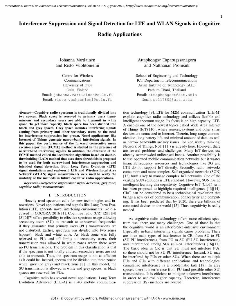
In modern CR, the spectrum is divided into three zones- white, grey and black. In Figure 1, zone classification ispresented. It is assumed that PU-SU distance is >y km in thewhite zone, <x km in the black zone, and in the grey zone itholds that x km <PU-SU-distance <y km [37]. It means that ifSU is more than y km from the PU, SU is allowed to transmit.If SU is closer than y km but further than x km from the PU,SU may be able to transmit with low power. Spectrum sensing

2



y-z km x-y km 0-x km

y kmz km x km

black

zone

grey

zone

white

zone

0 km

Figure 1: White, grey and black zones.

is required before transmission and there are interfering signalsso IS is needed to ensure SU transmissions. If PU-SU distanceis less than x km, SU transmission is not allowed.

Interference environment differs between the zones. Whitespace contains only noise. Therein, the noise is most com-monly additive white Gaussian (AWGN) noise at the receiver’sfront-end, and man-made noise. This is related to the used fre-quency band. Grey space contains interfering signals within thenoise, which causes challenges. Grey space is occupied by PU(and possible other SU) signals with low to medium power thatmeans interference with low to medium power. IS is requiredespecially is this zone. Black space includes communicationssignals, possible interfering signals, and noise. In black space,there are PU signals with high power and SUs have no access.

There must be some rules that enable SUs to transmit ingrey zone without causing any harm to PUs. According to [38],SU can transmit at the same time as PU if the limit of inter-ference temperature at the desired receiver is not reached. In[3], it is considered the maximum amount of interference thata receiver is able to tolerate, i.e., an interference temperaturemodel. This can be used when studying interference from SUto PU network. In [39], primary radio network (PRN) definessome interference margin. This can be done based on channelconditions and target performance metric. Interference marginis broadcasted to the cognitive radio network. In any case, themaximum transmit power of SUs is limited.

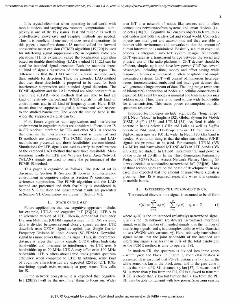
In our scenario presented in Figure 2, it is assumed thatwe have one PU base station (BS), several PU mobile stationsand several SUs. SU terminals form microcells. Part or all ofSUs are mobile and part of SUs may be intelligent devicesor sensors (i.e., IoT). Between SUs, weak signal powers areneeded for a transmission. One microcell can consist of, forexample, devices in an office room. They can use the same ordifferent signal types than PU. For example, in the office roomcase, WLAN can be used. Between the intelligent devices(IoT), UNB signals are used. It is assumed that SUs operateat grey zone, so IS is required to ensure the quality of SUtransmissions.

SUs measure signals transmitted by PU base stations andestimate relative distance to them. Using this information,SUs know whether their short range communication willcause harmful interference to the PU base station. To enablesecondary transmissions under continuous interference causedby the PU base station this interference is attenuated by IS.

The secondary access point knows the locations of PUterminals or SUs measure the power levels of the signals

Figure 2: Scenario with one macrocell and two microcells.

coming from PU mobile terminals in the uplink. If it isassumed that SUs know the locations of PUs, SUs do notinterfere with PUs. If SUs do not know PUs locations, theirtransmission is allowed when received PU signal power isbelow some predetermined threshold. If the level of the powercoming from a certain primary terminal is small, it is assumedthat secondary transmission generates negligible interferencetowards primary terminal. However, it may happen that SUsdon’t sense closely spaced silent PUs.

Let us consider microcell 1 in Figure 2. There are one SUtransmitter SU TX1 and four terminals SU i, i = 1, · · · , 4. Inaddition to the intended signal from SU TX1, SU 1 receivesthe noise η, SU 2 receives PU downlink (PU BS) signal andthe noise η, SU 3 receives PU downlink (PU BS) and PUuplink (PU 1) signals and the noise η, and SU 4 receives PUdownlink (PU BS) signal, signal from other microcell’s SU,and the noise η. That is, we get from (1) that

r1(n) = s(n) + η, (2)

r2(n) = s(n) + i2(n) + η, (3)

r3(n) = s(n) +

2∑j=1

ij(n) + η, (4)

r4(n) = s(n) +

3∑j=2

ij(n) + η, (5)

where i1(n) is PU 1, i2(n) is PU BS and i3(n) is other SU. Forexample, if it is assumed that PUs are in the LTE-A networkand SUs use WLAN signals, receiver SU 2 has to suppressOFDM signal, receiver SU 3 has to suppress OFDM and SC-FDMA signals, and receiver SU 4 has to suppress OFDM andWLAN signals.

In addition, interfering and communication (intended) sig-nals have to be separated from each other. The receiver has to

3



know what signals are interfering signals to be suppressed andwhat signals are of interest. In an ideal situation, detected andinterfering signals have distinct characteristics. However, this isnot always the situation. An easy way to separate an interferingsignal from the intended signal is to use different bandwidths.For example, in LTE networks, it is known that there are 6different signal bandwidths between 1.4 and 20 MHz that areused [9]. Especially if a different signal type is used, it is easyto separate interfering signals from our information signal. Itcan also be assumed that interfering signal has higher powerthan the desired signal. However, this consideration is out ofthe scope of this paper.

IV. INTERFERENCE SUPPRESSION

Interference suppression exploits the characteristics ofdesired/interfering signal by filtering the received signal[40]. After 1970, IS techniques have been widely studied.IS techniques include, for example, filters, cyclostationar-ity, transform-domain methods like wavelets and short-timeFourier transform (STFT), high order statistics, spatial process-ing like beamforming and joint detection/multiuser detection[41]. Filter-based IS is performed in the time domain. Thosecan be further divided into linear and nonlinear methods. Opti-mal filter (Wiener filter) can be defined only if the interferenceand signal of interest are known by their Power Spectral Den-sities (PSDs), which is only possible when they are stationary.Usually, the signal, the interference or both are nonstationary,so adaptive filtering is the alternative capable of tracking theircharacteristics. Linear predictive filters can be made adaptiveusing, for example, the least mean square (LMS) algorithm. Infilter-based IS, both computational complexity and hardwarecosts are low but co-channel interference cannot be suppressed,and no interference with similar waveforms to signals canbe suppressed. Cyclostationarity based IS has low hardwarecomplexity but medium computational complexity. This maycause challenges in real-time low-power applications.

In transform domain IS [42], signal is suppressed infrequency or in some other transform domain (like fractionalFourier transform). Usually, frequency domain is used, sosignal is transformed using the Fourier transform. Computa-tional complexity is medium, but transform domain IS cannotbe used when interference and signal-of-interest have thesame kind of waveforms and spectral power concentration.However, waveform design may be used. Transform domainIS has low hardware complexity. High-order statistics based ISis computationally complex, and multiple antennas/samplersare needed, so its hardware cost is high and computationalcomplexity too. In beamforming, co-channel interference aswell as interference with similar waveforms to the signal ofinterest can be suppressed, but because of multiple antennas,the hardware cost is high. Its computational complexity ismedium.

The less about the interfering signal characteristics isknown, the more demanding the IS task will be. As most ofthe IS methods need some information about the suppressedsignals and/or noise, there are some methods that are able tooperate blindly [19]. Blind IS methods do not need any a prioriinformation about the interfering signals, their modulations orother characteristics. Also, the noise level can be unknown, soit has to be estimated. Blind IS methods are well suited fordemanding and varying environments.

V. THE FCME AND THE LAD METHODS

The adaptively operating FCME method [19] was orig-inally proposed for impulsive IS in the time domain. Itwas noticed later that the method is practical also in thefrequency domain [20]. Earlier, the FCME method has mainlybeen studied against sinusoidal and impulsive signals that arenarrowband ones. The computational complexity of the FCMEmethod is N log2(N) due to the sorting [20]. Analysis of theFCME method has been presented in [20].

The FCME method adapts according to the noise level,so no information about the noise level is required. Becausethe noise is used as a basis of calculation, there is no needfor information about the suppressed signals. Even thoughit is assumed in the calculation that the noise is Gaussian,the FCME method operates even if the noise is not purelyGaussian [20]. In fact, it is sufficient that the noise differsfrom the signal. When it is assumed that the noise is Gaussian,x2 (=the energy of samples) has a chi-squared distributionwith two degrees of freedom. Thus, the used IS threshold iscalculated using [19]

Th = −ln(PFA,DES)x2 = TCMEx2, (6)

where TCME = −ln(PFA,DES) is the used pre-determinedthreshold parameter [20], PFA,DES is the desired false alarmrate used in constant false alarm rate (CFAR) methods,

x2 =1

Q

Q∑i=1

|xi|2 (7)

denotes the average sample mean, and Q is the size of theset. For example, when it is selected that PFA,DES = 0.1(=10% of the samples are above the threshold in the noise-only case), the threshold parameter TCME = −ln(0.1) = 2.3.In cognitive radio related applications, controlling PFA,DES isimportant, because PFA,DES is directly related to the loss ofspectral opportunities and caused interference [20]. Selectionof proper PFA,DES values is discussed more detailed in [20].The FCME method rearranges the frequency-domain samplesin an ascending order according to the sample energy, selects10% of the smallest samples to form the set Q, and calculatesthe mean of Q. After that, (6) is used to calculate the firstthreshold. Then, Q is updated to include all the samples belowthe threshold, a new mean is calculated, and a new thresholdis computed. This is continued until there are no new samplesbelow the threshold. Finally, samples above the threshold arefrom interfering signal(s) and suppressed.

The FCME algorithm is blind and it is independent ofmodulation methods, signal types and amounts of signals. Itcan be used in all frequency areas, from kHz to GHz. Theonly requirements are that (1) the signal(s) can not cover thewhole bandwidth under consideration, and (2) the signal(s)are above the noise level. The first requirement means that theFCME method can be used against RNB signals. For example,10 MHz signal is wideband when the studied bandwidth isthat 10 MHz, but RNB when the studied bandwidth is, e.g.,100 MHz. In fact, it is enough that the interfering signal doesnot cover more than 80% of the studied bandwidth. However,the narrower the interference is, the better the FCME methodoperates [43].

The LAD method [21] uses two FCME-thresholds in orderto enhance the detection capability of the FCME method

4



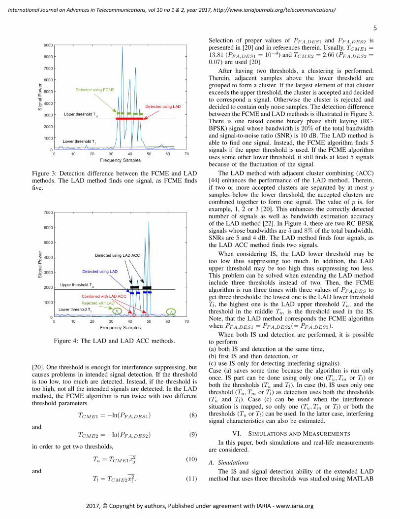
Figure 3: Detection difference between the FCME and LADmethods. The LAD method finds one signal, as FCME findsfive.

Figure 4: The LAD and LAD ACC methods.

[20]. One threshold is enough for interference suppressing, butcauses problems in intended signal detection. If the thresholdis too low, too much are detected. Instead, if the threshold istoo high, not all the intended signals are detected. In the LADmethod, the FCME algorithm is run twice with two differentthreshold parameters

TCME1 = −ln(PFA,DES1) (8)

andTCME2 = −ln(PFA,DES2) (9)

in order to get two thresholds,

Tu = TCME1x2j (10)

andTl = TCME2x2l . (11)

Selection of proper values of PFA,DES1 and PFA,DES2 ispresented in [20] and in references therein. Usually, TCME1 =13.81 (PFA,DES1 = 10−4) and TCME2 = 2.66 (PFA,DES2 =0.07) are used [20].

After having two thresholds, a clustering is performed.Therein, adjacent samples above the lower threshold aregrouped to form a cluster. If the largest element of that clusterexceeds the upper threshold, the cluster is accepted and decidedto correspond a signal. Otherwise the cluster is rejected anddecided to contain only noise samples. The detection differencebetween the FCME and LAD methods is illustrated in Figure 3.There is one raised cosine binary phase shift keying (RC-BPSK) signal whose bandwidth is 20% of the total bandwidthand signal-to-noise ratio (SNR) is 10 dB. The LAD method isable to find one signal. Instead, the FCME algorithm finds 5signals if the upper threshold is used. If the FCME algorithmuses some other lower threshold, it still finds at least 5 signalsbecause of the fluctuation of the signal.

The LAD method with adjacent cluster combining (ACC)[44] enhances the performance of the LAD method. Therein,if two or more accepted clusters are separated by at most psamples below the lower threshold, the accepted clusters arecombined together to form one signal. The value of p is, forexample, 1, 2 or 3 [20]. This enhances the correctly detectednumber of signals as well as bandwidth estimation accuracyof the LAD method [22]. In Figure 4, there are two RC-BPSKsignals whose bandwidths are 5 and 8% of the total bandwidth.SNRs are 5 and 4 dB. The LAD method finds four signals, asthe LAD ACC method finds two signals.

When considering IS, the LAD lower threshold may betoo low thus suppressing too much. In addition, the LADupper threshold may be too high thus suppressing too less.This problem can be solved when extending the LAD methodinclude three thresholds instead of two. Then, the FCMEalgorithm is run three times with three values of PFA,DES toget three thresholds: the lowest one is the LAD lower thresholdTl, the highest one is the LAD upper threshold Tu, and thethreshold in the middle Tm is the threshold used in the IS.Note, that the LAD method corresponds the FCME algorithmwhen PFA,DES1 = PFA,DES2(= PFA,DES3).

When both IS and detection are performed, it is possibleto perform(a) both IS and detection at the same time,(b) first IS and then detection, or(c) use IS only for detecting interfering signal(s).Case (a) saves some time because the algorithm is run onlyonce. IS part can be done using only one (Tu, Tm or Tl) orboth the thresholds (Tu and Tl). In case (b), IS uses only onethreshold (Tu, Tm or Tl) as detection uses both the thresholds(Tu and Tl). Case (c) can be used when the interferencesituation is mapped, so only one (Tu, Tm or Tl) or both thethresholds (Tu or Tl) can be used. In the latter case, interferingsignal characteristics can also be estimated.

VI. SIMULATIONS AND MEASUREMENTS

In this paper, both simulations and real-life measurementsare considered.

A. SimulationsThe IS and signal detection ability of the extended LAD

method that uses three thresholds was studied using MATLAB

5



Figure 5: Received signals at receiver. Intended signal and PU-SU interference, T=time and f=frequency.

0 1 2 3 4 5 6 7

Frequency [Hz] 109

0

1

2

3

4

5

6

7

Sig

nal p

ower

[Wat

t]

10-12

Interfering 16-QAM signalIntended 16-QAM signal

Figure 6: One intended 16-QAM signal and one interfering16-QAM signal. SNR=15 dB, SIR=12 dB.

simulations. In the simulations the focus was on the last 100meters at IoT network. There was a total of N devices, whichwere uniformly and independently deployed in a 2-dimensionalcircular plane with plane radius R. This deployment resultsin a 2-D Poisson point distribution of devices. After thenetwork was formed the devices were assumed to be static. Thenoise was additive white Gaussian noise (AWGN). The signalsand the noise were assumed to be uncorrelated. Here, 16-quadrature amplitude modulation (QAM) signal that transmits4 bits per symbol was used. It is one of the modulationtypes used in LTE. There were 1024 samples and fast Fouriertransformation (FFT) was used. In the simulations, IS anddetection were performed at the same time. IS was performedusing one threshold Tm = 6.9, as detection was performedusing two LAD thresholds Tu = 9.21 and Tl = 2.3. SNR isthe ratio of intended signal energy to noise power, as signal-to-interference ratio (SIR) is the ratio of intended signal energyto interfering signal energy.

The first situation is like (3), i.e., there is PU-SU in-

0 1 2 3 4 5 6 7

Frequency [Hz] 109

0

1

2

3

4

5

6

7

Sig

nal p

ower

[Wat

t]

10-12

Detected signal

Suppressed signal


Figure 7: One intended 16-QAM signal and one interfering16-QAM signal. After interference suppression and detection.SNR=15 dB, SIR=12 dB.

0 1 2 3 4 5 6 7 109

Frequency [Hz]

0

1

2

3

4

5

6

7S

igna

l Pow

er [W

att]

10-12


Figure 8: One intended 16-QAM signal and one interfering16-QAM signal. SNR=12 dB, SIR=15 dB.

terference (Figure 5). Thus, the received signal is of formr2(n) = s(n) + i2(n) + η, where s(n) and i2(n) are both16-QAM signals. Now, s(n) is intended signal (red arrow)as i2(n) is interfering signal from PU (blue arrow). Theirbandwidth covers about 30% of the total bandwidth. In Fig-ure 6, SNR=15 dB and SIR=12 dB, so intended signal isstronger than interfering signal. Figure 7 shows the situationafter interference suppression and signal detection. In Figure 8,SNR=12 dB and SIR=15 dB more, so intended signal is weakerthan interfering signal. The situation after signal detection andIS is illustrated in Figure 9. It can be said that both the methodsperform well.

Next, r4(n) = s(n) +∑3j=2 ij(n) + η like in (5). Now

6



0 1 2 3 4 5 6 7 109

Frequency [Hz]

0

1

2

3

4

5

6

7S

igna

l Pow

er [W

att]

10-12

Suppressed signal

Detected signal


Figure 9: One intended 16-QAM signal and one interfering16-QAM signal. After interference suppression and detection.SNR=12 dB, SIR=15 dB.

Figure 10: Received signals at receiver. Intended signal, PU-SU and SU-SU interference, T=time and f=frequency.

there are two suppressed signals: one is from PU and one isfrom other SU so there is both PU-SU and SU-SU interference(Figure 10). Now, s(n) is intended signal (red arrow), i2(n)is interfering signal from PU (blue arrow), and i3(n) is inter-fering signal from other SU (green arrow). Their bandwidthcovers about 45% of the total bandwidth. In Figure 11, all thethresholds Tu, Tl and Tm are presented. As the intended signalis detected using theresholds Tu and Tl, the IS is performedusing threshold Tm. As can be seen, all the signals are foundand both the interfering signals are suppressed.

B. MeasurementsThe IS performance of the FCME method against RNB

signals was studied using real-world wireless data. The re-sults are based on real-life measurements. Measurements wereperformed using spectrum analyzer Agilent E4446 [45] (Fig-ure 12). Three types of signals were studied, namely theLTE uplink, LTE downlink, and WLAN signals. All thosesignals are commonly used wireless signals. Both LTE1800

0 1 2 3 4 5 6

Frequency [Hz] 109

0

0.5

1

1.5

2

2.5

3

3.5

4

Sig

nal p

ower

[Wat

t]

10-12

Upper threshold Tu

Lower threshold Tl

Middle threshold Tm

Detected signalSuppressed signals


Figure 11: One intended 16-QAM signal and two interfering16-QAM signals. Interference suppression (Tm) and detection(Tu and Tl) thresholds. SNR=15 dB, SIR=12 dB.

Figure 12: Agilent E4446. LTE1800 network downlink signals.

network frequencies and WLAN signals were measured atthe University of Oulu, Finland. IS was performed using theFCME method with threshold parameter 4.6, i.e., desired falsealarm rate PFA,DES = 1% = 0.01 [20].

LTE1800 network operates at 2 × 75 MHz band so thatuplink is on 1.710− 1.785 GHz and downlink is on 1.805−1.880 GHz [46]. LTE downlink uses OFDM signal as uplinkuses SC-FDMA. LTE assumes a small nominal guard band(10% of the band, excluding 1.4 MHz case).

One measurement at 1.7− 1.9 GHz containing 1000 timedomain sweeps and 1601 frequency domain points is seen inFigure 13. Therein, yellow means strong signal power (=signal)as green means weaker signal power (=noise). Therein, onlydownlink signaling is present. Downlink signals have largerinterference distance than uplink signals. Interfering signalscover about 30% of the studied bandwidth. In Figure 14,situation after the FCME IS is presented. Therein, yellowmeans strong signal power as white means no signal power.It can be seen that the signals (white) have been suppressedand the noise is now dominant (yellow). On uplink signalfrequencies where no signals are present (600 first frequency

7



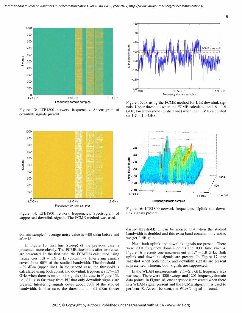
Figure 13: LTE1800 network frequencies. Spectrogram ofdownlink signals present.

Figure 14: LTE1800 network frequencies. Spectrogram ofsuppressed downlink signals. The FCME method was used.

domain samples), average noise value is −99 dBm before andafter IS.

In Figure 15, first line (sweep) of the previous case ispresented more closely. The FCME thresholds after two casesare presented. In the first case, the FCME is calculated usingfrequencies 1.8 − 1.9 GHz (downlink). Interfering signalscover about 60% of the studied bandwidth. The threshold is−89 dBm (upper line). In the second case, the threshold iscalculated using both uplink and downlink frequencies 1.7−1.9GHz when there is no uplink signals (like case in Figure 13),i.e., SU is so far away from PU that only downlink signals arepresent. Interfering signals cover about 30% of the studiedbandwidth. In that case, the threshold is −91 dBm (lower

1.8 GHz 1.85 GHz 1.9 GHz−130

−120

−110

−100

−90

−80

−70

−60

Frequency domain samples

Sig

nal p

ower

[dB

m]

FCME threhsold

Figure 15: IS using the FCME method for LTE downlink sig-nals. Upper threshold when the FCME calculated on 1.8−1.9GHz, lower threshold (dashed line) when the FCME calculatedon 1.7− 1.9 GHz.

Figure 16: LTE1800 network frequencies. Uplink and down-link signals present.

dashed threshold). It can be noticed that when the studiedbandwidth is doubled and this extra band contains only noise,we get 2 dB gain.

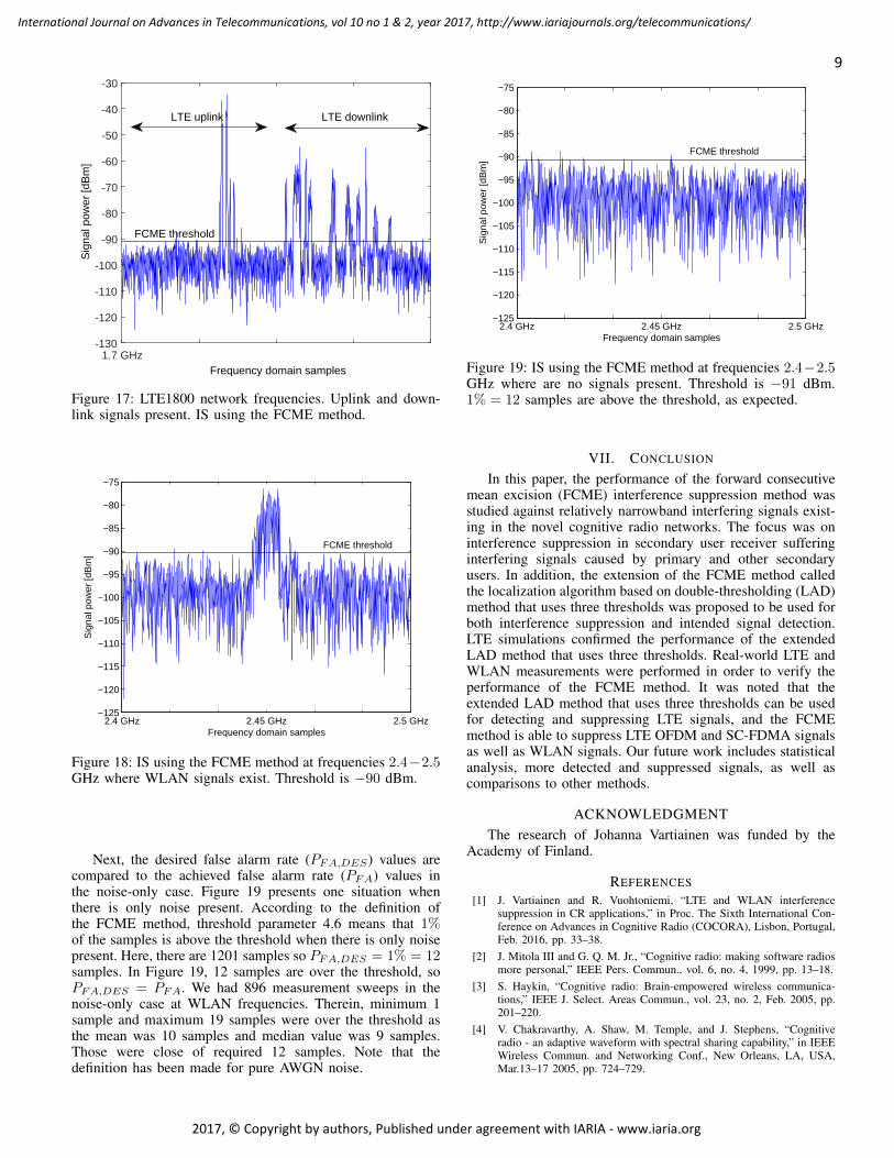
Next, both uplink and downlink signals are present. Therewere 2001 frequency domain points and 1000 time sweeps.Figure 16 presents one measurement at 1.7 − 1.9 GHz. Bothuplink and downlink signals are present. In Figure 17, onesnapshot when both uplink and downlink signals are presentis presented. Therein, both signals are suppressed.

In the WLAN measurements, 2.4−2.5 GHz frequency areawas used. There were 1000 sweeps and 1201 frequency domaindata points. In Figure 18, one snapshot is presented when thereis a WLAN signal present and the FCME algorithm is used toperform IS. As can be seen, the WLAN signal is found.

8



1.7 GHzFrequency domain samples

-130

-120

-110

-100

-90

-80

-70

-60

-50

-40

-30S

igna

l pow

er [d

Bm

]

FCME threshold

LTE uplink LTE downlink

Figure 17: LTE1800 network frequencies. Uplink and down-link signals present. IS using the FCME method.

2.4 GHz 2.45 GHz 2.5 GHz−125

−120

−115

−110

−105

−100

−95

−90

−85

−80

−75


Sig

nal p

ower

[dB

m]

FCME threshold

Figure 18: IS using the FCME method at frequencies 2.4−2.5GHz where WLAN signals exist. Threshold is −90 dBm.

Next, the desired false alarm rate (PFA,DES) values arecompared to the achieved false alarm rate (PFA) values inthe noise-only case. Figure 19 presents one situation whenthere is only noise present. According to the definition ofthe FCME method, threshold parameter 4.6 means that 1%of the samples is above the threshold when there is only noisepresent. Here, there are 1201 samples so PFA,DES = 1% = 12samples. In Figure 19, 12 samples are over the threshold, soPFA,DES = PFA. We had 896 measurement sweeps in thenoise-only case at WLAN frequencies. Therein, minimum 1sample and maximum 19 samples were over the threshold asthe mean was 10 samples and median value was 9 samples.Those were close of required 12 samples. Note that thedefinition has been made for pure AWGN noise.

2.4 GHz 2.45 GHz 2.5 GHz−125

−120

−115

−110

−105

−100

−95

−90

−85

−80

−75


Sig

nal p

ower

[dB

m]

FCME threshold

Figure 19: IS using the FCME method at frequencies 2.4−2.5GHz where are no signals present. Threshold is −91 dBm.1% = 12 samples are above the threshold, as expected.

VII. CONCLUSION

In this paper, the performance of the forward consecutivemean excision (FCME) interference suppression method wasstudied against relatively narrowband interfering signals exist-ing in the novel cognitive radio networks. The focus was oninterference suppression in secondary user receiver sufferinginterfering signals caused by primary and other secondaryusers. In addition, the extension of the FCME method calledthe localization algorithm based on double-thresholding (LAD)method that uses three thresholds was proposed to be used forboth interference suppression and intended signal detection.LTE simulations confirmed the performance of the extendedLAD method that uses three thresholds. Real-world LTE andWLAN measurements were performed in order to verify theperformance of the FCME method. It was noted that theextended LAD method that uses three thresholds can be usedfor detecting and suppressing LTE signals, and the FCMEmethod is able to suppress LTE OFDM and SC-FDMA signalsas well as WLAN signals. Our future work includes statisticalanalysis, more detected and suppressed signals, as well ascomparisons to other methods.

ACKNOWLEDGMENTThe research of Johanna Vartiainen was funded by the

Academy of Finland.

REFERENCES

[1] J. Vartiainen and R. Vuohtoniemi, “LTE and WLAN interferencesuppression in CR applications,” in Proc. The Sixth International Con-ference on Advances in Cognitive Radio (COCORA), Lisbon, Portugal,Feb. 2016, pp. 33–38.

[2] J. Mitola III and G. Q. M. Jr., “Cognitive radio: making software radiosmore personal,” IEEE Pers. Commun., vol. 6, no. 4, 1999, pp. 13–18.

[3] S. Haykin, “Cognitive radio: Brain-empowered wireless communica-tions,” IEEE J. Select. Areas Commun., vol. 23, no. 2, Feb. 2005, pp.201–220.

[4] V. Chakravarthy, A. Shaw, M. Temple, and J. Stephens, “Cognitiveradio - an adaptive waveform with spectral sharing capability,” in IEEEWireless Commun. and Networking Conf., New Orleans, LA, USA,Mar.13–17 2005, pp. 724–729.

9



[5] S. N. Shankar, C. Cordeiro, and K. Challapali, “Spectrum agile radios:Utilization and sensing architectures,” in IEEE Int. Symposium on Dy-namic Spectrum Access Networks (DySpAN) 2005, vol. 1, Baltimore,USA, Nov. 2005, pp. 160–169.

[6] T. Yucek and H. Arslan, “A survey of spectrum sensing algorithms forcognitive radio applications,” IEEE Commun. Surveys and Tutorials,vol. 11, no. 1, 2009, pp. 116–130.

[7] J. Mitola III, “Cognitive radio architecture evolution,” IEEE Proceed-ings, vol. 97, no. 4, 2009, pp. 626–641.

[8] S. Haykin, D. J. Thomson, and J. H. Reed, “Spectrum sensing for cog-nitive radio - the utility of the multitaper method and cyclostationarityfor sensing the radio spectrum, including the digital tv spectrum, isstudied theoretically and experimentally,” Proc. of the IEEE, vol. 97,no. 5, May 2009, pp. 849–877.

[9] 3GPP, “The mobile broadband standard,” (2013), http://www.3gpp.org[retrieved: May, 2017].

[10] K. Ashton, “That ’internet of things’ thing,” RFID Journal, June 2009,http://www.rfidjournal.com/articles/view?4986 [retrieved: May, 2017].

[11] J. Voas, “Networks of ’things’,” NIST Special Publication 800-183,July 2016. http://dx.doi.org/10.6028/NIST. SP.800-183 [retrieved: May,2017].

[12] O.-C. Iacoboaiea, B. Sayrac, S. B. Jemaa, and P. Bianchi, “SON coordi-nation in heterogenous networks: A reinforcement learning framework,”IEEE Trans. Wirel. Commun., vol. 15, no. 9, 2016, pp. 5835–5847.

[13] R. F. Shigueta, M. Fonseca, A. C. Viana, A. Ziviani, and A. Munaretto,“A strategy for opportunistic cognitive channel allocation in wirelessinternet of things,” in IFIP Wireless Days, Rio de Janeiro, Brazil, Nov2014.

[14] A. Alja and A. H. Aghvami, “Cognitive machine-to-machine communi-cations for internet-of-things: A protocol stack perspective,” IEEE IoTJournal, vol. 2, no. 2, 2016, pp. 103–112.

[15] A. Nordrum, “Popular internet of things forecast of 50 billiondevices by 2020 is outdated,” in IEEE Spectrum, Aug. 2016,http://spectrum.ieee.org/tech-talk/telecom/internet/popular-internet-of-things-forecast-of-50-billion-devices-by-2020-is-outdated [retrieved:May, 2017].

[16] Z. Chen, “Interference modelling and management for cogni-tive radio networks,” Ph.D. dissertation, Doctoral Thesis (sub-mitted), Apr. 2011, http://www.ros.hw.ac.uk/bitstream/10399/2421/1/ChenZ 0511 eps.pdf [retrieved: May, 2017].

[17] K. Nishimori, H. Yomo, and P. Popovski, “Distributed interferencecancellation for cognitive radios using periodic signals of the primarysystem,” IEEE Trans. Wirel. Commun., vol. 10, no. 9, 2011, pp. 2971– 2981.

[18] J. Peha, “Spectrum sharing in the gray space,” TelecommunicationsPolicy Journal, vol. 37, no. 2-3, 2013, pp. 167–177.

[19] H. Saarnisaari, P. Henttu, and M. Juntti, “Iterative multidimensionalimpulse detectors for communications based on the classical diagnosticmethods,” IEEE Trans. Commun., vol. 53, no. 3, Mar. 2005, pp. 395–398.

[20] J. Vartiainen, “Concentrated signal extraction using consecutive meanexcision algorithms,” Ph.D. dissertation, Acta Univ Oul Technica C 368.Faculty of Technology, University of Oulu, Finland, Nov. 2010, http://jultika.oulu.fi/Record/isbn978-951-42-6349-1 [retrieved: May, 2017].

[21] J. Vartiainen, J. J. Lehtomaki, and H. Saarnisaari, “Double-thresholdbased narrowband signal extraction,” in Proc. IEEE Veh. Technol. Conf.(VTC) 2005, Stockholm, Sweden, May/June 2005, pp. 1288–1292.

[22] J. Vartiainen, J. J. Lehtomaki, H. Saarnisaari, and M. Juntti, “Two-dimensional signal localization algorithm for spectrum sensing,” IEICETrans. Commun., vol. E93-B, no. 11, Nov. 2010, pp. 3129–3136.

[23] J. A. Stankovic, “Research directions for the internet of things,” IEEEInt. of Things Journal, vol. 1, no. 1, Feb. 2014, pp. 3–9.

[24] A. H. Ngu, M. Gutierrez, V. Metsis, S. Nepal, and Q. Z. Sheng, “IoTmiddleware: A survey on issues and enabling technologies,” IEEE Int.of Things Journal, vol. 4, no. 1, Feb. 2017, pp. 1–20.

[25] P. Karunakaran, T. Wagner, A. Scherb, and W. Gerstacker, “Sensing forspectrum sharing in cognitive LTE-A cellular networks,” cornell Uni-versity Library. http://arxiv.org/abs/1401.8226 [retrieved: May, 2017].

[26] L. Zhang, L. Yang, and T. Yang, “Cognitive interference managementfor LTE-A femtocells with distributed carrier selection,” in Proc. IEEEVeh. Technol. Conf. (VTC) Fall, 2010, pp. 1–5.

[27] V. Osa, C. Hearranz, J. F. Monserrat, and X. Gelabert, “Implementingopportunistic spectrum access in LTE-advanced,” EURASIP Journal onWireless Communications and Networking, vol. 99, 2012, pp. 1–17.

[28] Q. Wu et al., “Cognitive internet of things: A new paradigm beyondconnection,” IEEE Journal of Internet of Things, vol. 1, no. 2, 2014,pp. 1–15, [retrieved: May, 2017].

[29] J. Tervonen, K.Mikhaylov, S. Pieska, J. Jamsa, and M.Heikkila, “Cogni-tive internet-of-things solutions enabled by wireless sensor and actuatornetworks,” in IEEE Conf. on Cognitive Infocommun. (CogInfoCom),2014, pp. 97–102.

[30] F. Xia, L. T. Yang, L. Wang, and A. Vine, “Internet of things,” Int.Journal of Commun. Systems, vol. 25, 2012, pp. 1101–1102.

[31] LoRa, http://lora-alliance.org/ [retrieved: May, 2017].[32] Neul, www.neul.com [retrieved: May, 2017].[33] SigFox, www.sigfox.com [retrieved: May, 2017].[34] Nokia, “LTE M2M - optimizing LTE for the internet of things,” in White

paper, 2014, http://networks.nokia.com/file/34496/lte-m-optimizing-lte-for-the-internet-of-things [retrieved: May, 2017].

[35] J. Gozalvez, “New 3GPP standarf for IoT,” IEEE Vehicular TechnologyMagazine, vol. 11, no. 1, Mar. 2016, pp. 14–20.

[36] 3GPP16, “Standardization of NB-IOT completed,” (2016),http://www.3gpp.org/news-events/3gpp-news [retrieved: May, 2017].

[37] Z. Feng and Y. Xu, “Cognitive TD-LTE system operatingin TV white space in china,” ITU-R WP 5A, Geneva,Switzerland, (2013), http://studylib.net/doc/13258156/cognitive-td-lte-system-operating-in-tv-white-space-in-china[retrieved: May, 2017].

[38] J. Mitra and L. Lampe, “Sensing and suppression of impulsive interfer-ence,” in Canadian Conference on Electrical and Computer Engineering(CCECE), Canada, May 2009, pp. 219–224.

[39] Y. Ma, D. I. Kim, and Z. Wu, “Optimization of OFDMA-based cellularcognitive radio networks,” IEEE Trans. on Commun., vol. 58, no. 8,2010, pp. 2265–2276.

[40] J. Andrews, “Interference cancelation for cellular systems: a contempo-rary overview,” IEEE Wireless Comm., vol. 12, no. 2, Apr. 2005, pp.19–29.

[41] X. Hong, Z. Chen, C.-X. Wang, S. A. Vorobyov, and J. S. Thompson,“Cognitive radio networks - interference cancelation and managementtechniques,” IEEE Veh. Technol. Magazine, Dec. 2009, pp. 76–84.

[42] L. B. Milstein and P. K. Das, “An analysis of a real-time transformdomain filtering digital communication system - part I: Narrowbandinterference rejection using eral-time Fourier transforms,” IEEE Trans.Commun., vol. 28, 1980, pp. 816–824.

[43] J. Vartiainen, J. J. Lehtomaki, H. Saarnisaari, and M. Juntti, “Analysisof the consecutive mean excision algorithms,” J. Elect. Comp. Eng.,2011, pp. 1–13.

[44] J. Vartiainen, H. Sarvanko, J. Lehtomaki, M. Juntti, and M. Latva-aho,“Spectrum sensing with LAD based methods,” in Proc. IEEE Int. Symp.Pers., Indoor, Mobile Radio Commun. (PIMRC), Athens, Greece, Aug.2007, pp. 1–5.

[45] Agilent, http://www.agilent.com [retrieved: May, 2017].[46] Nokia Siemens Networks, “Introducing LTE with max-

imum reuse of GSM assets,” in White paper, 2011,http://www.gsma.com/spectrum/introducing-lte-with-maximum-reuse-of-gsm-asset/ [retrieved: May, 2017].

10



Impact of Analytics and Meta-learning on Estimating Geomagnetic StormsA Two-stage Framework for Prediction

Taylor K. Larkin1 and Denise J. McManus2Information Systems, Statistics, and Management Science

Culverhouse College of CommerceThe University of AlabamaTuscaloosa, AL 35487-0226

Email: [email protected], [email protected]

Abstract—Cataclysmic damage to telecommunication infrastruc-tures, from power grids to satellites, is a global concern. Nat-ural disasters, such as hurricanes, tsunamis, floods, mud slides,and tornadoes have impacted telecommunication services whilecosting millions of dollars in damages and loss of business.Geomagnetic storms, specifically coronal mass ejections, have thesame risk of imposing catastrophic devastation as other naturaldisasters. With increases in data availability, accurate predictionscan be made using sophisticated ensemble modeling schemes. Inthis work, one such scheme, referred to as stacked generalization,is used to predict a geomagnetic storm index value associatedwith 2,811 coronal mass ejection events that occurred between1996 and 2014. To increase lead time, two rounds (stages) ofstacked generalization using data relevant to a coronal massejection’s life span are executed. Results show that for this dataset,stacked generalization performs significantly better than usinga single model in both stages for the most important errormetrics. In addition, overall variable importance scores for eachpredictor variable can be calculated from this ensemble strategy.Utilizing these importance scores can help aid telecommunicationresearchers in studying the significant drivers of geomagneticstorms while also maintaining predictive accuracy.

Keywords–ensemble modeling; space weather; quantile regres-sion; stacked generalization; telecommunications.

I. INTRODUCTION

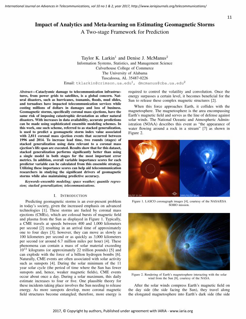
Predicting geomagnetic storms is an ever-present problemin today’s society, given the increased emphasis on advancedtechnologies [1]. These storms are fueled by coronal massejections (CMEs), which are colossal bursts of magnetic fieldand plasma from the Sun as displayed in Figure 1. Typically,a CME travels at speeds between 400 and 1,000 kilometersper second [2] resulting in an arrival time of approximatelyone to four days [3]; however, they can move as slowly as100 kilometers per second or as quickly as 3,000 kilometersper second (or around 6.7 million miles per hour) [4]. Thesephenomena can contain a mass of solar material exceeding1013 kilograms (or approximately 22 trillion pounds) [5] andcan explode with the force of a billion hydrogen bombs [6].Naturally, CME events are often associated with solar activitysuch as sunspots [4]. During the solar minimum of the 11year solar cycle (the period of time where the Sun has fewersunspots and, hence, weaker magnetic fields), CME eventsoccur about once a day. During a solar maximum, this dailyestimate increases to four or five. One plausible theory forthese incidents taking place involves the Sun needing to releaseenergy. As more sunspots develop, more coronal magneticfield structures become entangled; therefore, more energy is

required to control the volatility and convolution. Once theenergy surpasses a certain level, it becomes beneficial for theSun to release these complex magnetic structures [2].

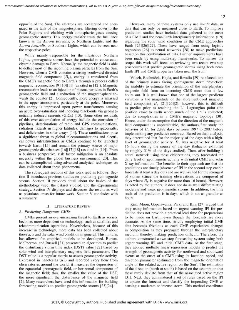
When this force approaches Earth, it collides with themagnetosphere. The magnetosphere is the area encompassingEarth’s magnetic field and serves as the line of defense againstsolar winds. The National Oceanic and Atmospheric Admin-istration (NOAA) describes this event as “the appearance ofwater flowing around a rock in a stream” [7] as shown inFigure 2.

Figure 1. LASCO coronagraph images [4], courtesy of the NASA/ESASOHO mission.

Figure 2. Rendering of Earth’s magnetosphere interacting with the solarwind from the Sun [8], courtesy of the NASA.

After the solar winds compress Earth’s magnetic field onthe day side (the side facing the Sun), they travel alongthe elongated magnetosphere into Earth’s dark side (the side

11



opposite of the Sun). The electrons are accelerated and ener-gized in the tails of the magnetosphere, filtering down to thePolar Regions and clashing with atmospheric gases causinggeomagnetic storms. This energy transfer emits the brillianceknown as the Aurora Borealis, or Northern Lights, and theAurora Australis, or Southern Lights, which can be seen nearthe respective poles.

While mainly responsible for the illustrious NorthernLights, geomagnetic storms have the potential to cause cata-clysmic damage to Earth. Normally, the magnetic field is ableto deflect most of the incoming plasma particles from the Sun.However, when a CME contains a strong southward-directedmagnetic field component (Bz), energy is transferred fromthe CME’s magnetic field to Earth’s through a process calledmagnetic reconnection [9][10][11] (as cited in [12]). Magneticreconnection leads to an injection of plasma particles in Earth’sgeomagnetic field and a reduction of the magnetosphere to-wards the equator [2]. Consequently, more energy is amassedin the upper atmosphere, particularly at the poles. Moreover,this energy is impressed upon power transformers causingan acute over-saturation and inducing black-outs via geomag-netically induced currents (GICs) [13]. Some other residualsof this over-accumulation of energy include the corrosion ofpipelines, deteriorations of radio and GPS communications,radiation hazards in higher latitudes, damages to spacecrafts,and deficiencies in solar arrays [14]. These ramifications posea significant threat to global telecommunications and electri-cal power infrastructures as CMEs continue to be launchedtowards Earth [15] and remain the primary source of majorgeomagnetic disturbances [16][17][18] (as cited in [19]). Froma business perspective, risk factor mitigation is an absolutenecessity within the global business environment [20]. Thiscan be accomplished using advanced analytical techniques ondata collected about these phenomena.

The subsequent sections of this work read as follows. Sec-tion II introduces previous studies on predicting geomagneticstorms. Section III provides detail about the basics of themethodology used, the dataset studied, and the experimentalstrategy. Section IV displays and discusses the results as wellas postulates areas for future work. Section V concludes witha summary.

II. LITERATURE REVIEW

A. Predicting Dangerous CMEsCMEs present an ever-increasing threat to Earth as society

becomes more dependent on technology, such as satellites andtelecommunication operations. Nevertheless, because of thisincrease in technology, more data has been collected aboutthese acts and the solar wind condition in general. This, in turn,has allowed for empirical models to be developed. Burton,McPherron, and Russell [21] presented an algorithm to predictthe disturbance storm time index (DST) value [22] based onsolar wind and interplanetary magnetic field parameters. TheDST value is a popular metric to assess geomagnetic activity.Expressed in nanoteslas (nT) and recorded every hour fromobservatories around the world, it measures the depression ofthe equatorial geomagnetic field, or horizontal component ofthe magnetic field; thus, the smaller the value of the DST,the more significant the disturbance of the magnetic field[2]. Many researchers have used this information for buildingforecasting models to predict geomagnetic storms [23][24].

However, many of these systems only use in-situ data, ordata that can only be measured close to Earth. To improveprediction, studies have included data gathered at the onsetof a CME and the near-Earth interplanetary information (IPI)regarding the solar wind condition as the CME approachesEarth [25][26][27]. These have ranged from using logisticregression [26] to neural networks [28] to make predictionsbased on this combination of data. Further improvements havebeen made by using multi-step frameworks. To narrow thescope, this work will focus on reviewing two recent two-stepprocedures that predict geomagnetic storms using both near-Earth IPI and CME properties taken near the Sun.

Valach, Bochnıcek, Hejda, and Revallo [29] reinforced oneof the primary issues facing geomagnetic storm prediction:the inability to estimate the orientation of the interplanetarymagnetic field from an incoming CME more than a fewhours out. It is well-known that one of the largest predictorvariables is the magnitude of the aforementioned magneticfield component Bz [21][26][2]; however, this is difficultto predict prior to reaching the L1 Lagrangian point (theposition close to Earth where much of the IPI is collected)due to complexities in a CME’s magnetic topology [30].Hence, under the assumption that the direction of the magneticfield component is unpredictable, the authors first study thebehavior of Bz for 2,882 days between 1997 to 2007 beforeimplementing any predictive construct. Based on their analysis,they determined that for the majority of the days with a high-level of geomagnetic activity, Bz was negative for at least16 hours during the course of the day (behavior exhibitedby roughly 31% of the days studied). Then, after building aneural network using these observations, they forecasted thedaily level of geomagnetic activity with initial CME and solarX-ray information. The benefits to their approach are that thepredictions are timely (absence of IPI in the second step enableforecasts at least a day out) and are well-suited for the strongestof storms (since the training observations are composed ofdays where Bz is negative for more than 16 hours). However,as noted by the authors, it does not do as well differentiatingmoderate and weak geomagnetic storms. In addition, the timescale of the prediction is in days, which is not as granular ashours.

Kim, Moon, Gopalswamy, Park, and Kim [27] argued thatonly using information based on urgent warning IPI for pre-diction does not provide a practical lead time for preparationsto be made on Earth, even though the forecasts are moreaccurate. At the same time, strictly employing initial CMEdata becomes frivolous as each CME experiences changesin composition as they propagate through the interplanetarymedium, thereby, making prediction difficult. Therefore, theauthors constructed a two-step forecasting system using bothurgent warning IPI and initial CME data. At the first stage,they applied multiple linear regression models to predict thestrength of geomagnetic activity for northward and southwardevents at the onset of a CME using its location, speed, anddirection parameter (estimated from the magnetic orientationangle of the related active region on the Sun). The estimationof the direction (north or south) is based on the assumption thatthese rarely deviate from that of the associated active region[31]. Next, they administered a set of rules based on the IPIto update the forecast and classify the impending CME ascausing a moderate or intense storm. This method contributes

12



a medium-term to short-term forecast from the first observanceof a CME to its approach to Earth. While this method yieldsaccurate and interpretable results, only 55 CMEs from 1997-2003 were studied. Moreover, the absence of using a validationscheme when creating the rules can lead to over-fitting whenpredicting on future data [32].

Interestingly enough, the former work assumes the direc-tion of the magnetic field component in a CME is unpredictablewhile the latter estimates this in their step one models. Inthis work, the direction is not considered in any of the steps.Instead, the dataset captures values of Bz prior to the climaxof a given geomagnetic storm [33]. Thus, if this value is highin magnitude, then this reflects the southward behavior.

Aside from the work by Dryer et al. [25], which usedan ensemble of four physics-based models to predict shockarrival times, the idea of using ensembles of models has notbeen very prevalent in the literature. Stacked generalization[34] is a type of ensemble that uses the individual predictionsfrom a set of base models as inputs for another model tomake a final prediction. This strategy has been the backboneof successful schemes in areas such as predicting financialfraud [35], bankruptcy [36], and user ratings in the famousNetflix Prize competition [37]. Therefore, leveraging moreadvanced ensemble frameworks for predictive modeling hasthe opportunity to increase accuracy in this field.

B. Stacked GeneralizationThe idea of stacked generalization can be simplified in the

following way:

• Construct a dataset consisting of predictions from aset of level 0 (or base) learners using a training and atest set. Refer to this as the metadata.

• Generate a level 1 (or meta) learner that utilizes thepredictions made at the previous level as inputs. Thatis, train the meta-learner on the metadata as opposedto the original training data.

Often times, the predictions from the base-learners are de-termined via k-fold cross-validation [38]. Define the datasetS = {(yi,xi), i = 1, ..., n} where xi is a vector of predictorvariables and yi is the corresponding response value for the ithobservation. Specifically, split the dataset S into k near equaland disjoint sets such that S1, S2, ..., Sk. Let S−k = S−Sk andSk be the training and test sets, respectively. Execute the base-learner on the first S−k parts and produce a prediction for theheld-out part Sk. Repeat this procedure until each subset of Shas been used as a test set exactly once. Extract all the hold-out predictions to create the metadata. Because generating themetadata is an independent process across each base-learner, itcan be parallelized for faster computation. That is, each base-learner can be trained at the same time. This is key as timeplays a pivotal role in geomagnetic storm prediction [27].

The meta-learner’s purpose is to gain information aboutthe generalization behavior of each learner trained at the base-level. Popular choices for meta-learners have been linear mod-els [39]. While this ensemble strategy leverages the strengthsand weaknesses of the base-learners, it can be prone to over-fitting [40]. Therefore, in order to combat this issue, employingregularized linear methods can perform better than their non-regularized counterparts [41][38][42]. Reid and Grudic [42]experimented with three regularization penalties: ridge [43],

lasso [44], and the elastic net [45]. The authors showed thatimposing these penalties perform well on multi-class datasets.They commented that using the lasso and elastic net penaltiescan promote sparse solutions that can reduce the size of theensemble at the meta-level. Pruning the size of an ensemblemodel has been explored in other works [46][47][48]. Itcan lead to better generalization and promote the necessarydiversity in the base-learner predictions [34].

Based upon the results in previous studies, it seems ad-vantageous to implement a regularized meta-learner to havethe best potential for success in stacked generalization. Byusing various types of penalty functions, a learning system caneffectively make predictions and provide sparse solutions, evenin situations with severe multicollinearity since all of the base-learners are trying to predict the same outcome [38]. However,none of the studies mentioned above discuss how to choosea meta-learner when the outlier values are important for re-gression tasks. Specifically for predicting geomagnetic storms,outliers are important because strong CMEs do not occur often;hence, a meta-learner cannot downplay the effect of thesefor prediction. If anything, the meta-learner should treat thesevalues with more emphasis. In addition, subsetting the datato only include these outliers for model construction inhibitsmeta-knowledge to be gained for all CME events. Therefore,for this study, a regularized quantile regression model is chosenfor the meta-learner in order to more adequately deal withoutliers, improve accuracy, and promote sparse solutions.

C. Regularized Quantile RegressionRecall the ordinary least squares (OLS) solution for the

coefficients in linear regression:

βols = (X ′X)−1X ′Y (1)

where X is the predictor matrix of dimension n × (p + 1)and Y is the vector of outcomes of dimension n × 1 for nobservations and p predictor variables. Specifically,

X =

1 x11 x12 . . . x1p1 x21 x22 . . . x2p

1...

.... . .

...1 xn1 xn2 . . . xnp

Y =

y1y2...yn

Alternatively, Eq. (1) can be written as the following optimiza-tion problem:

argminβ

1

n

n∑i=1

(yi − x′iβ)2 (2)

To apply regularization to the estimated coefficients, a penaltyterm can be added such that [49]

argminβ

1

n

n∑i=1

(yi − x′iβ)2 +p∑j=1

pλ(|βj |) (3)

where pλ(·) dictates the type of penalty function with a non-negative constant λ to determine the amount of regulariza-tion. Utilizing constrained regression approaches enables theability to perform variable selection or improve predictionin particular environments. However, the main goal in thesemethods is to estimate the conditional mean of some responsegiven a set of predictor variables. Situations may arise whereit is more advantageous to investigate a certain part of the

13



conditional distribution [50][51]; hence, quantile regressionwas developed [52]. The goal of quantile regression is tooffer “a comprehensive strategy for completing the regressionpicture” (pg. 20) [53]. In general, this involves minimizing thesum of asymmetrically weighted absolute residuals [52]

argminβ

1

n

[ ∑i∈{i:yi≥x′iβ}

τ |yi − x′iβ|

+∑

i∈{i:yi<x′iβ}

(1− τ)|yi − x′iβ|] (4)

for some given quantile level τ . In this way, different weightsare placed on positive (under-prediction) and negative (over-prediction) errors corresponding to the desired quantile. Notethat when τ = 0.5, this simply reduces to median regression.As with the linear case, the coefficients in quantile regressioncan be penalized the same way. Using lasso has been apopular choice due to its sparse nature [54][55]. However,it has been shown that lasso has some limitations in high-dimensional situations or ones with severe multicollinearity[45]. In addition, it lacks oracle properties [56][57]. That is,lasso does not select the correct subset of predictor variableswhile also efficiently estimating the non-zero coefficients as ifonly the truly influential predictor variables are included in themodel, asymptotically [58]. Thus other penalties, such as thesmoothly clipped absolute deviation (SCAD) [56], have beendeveloped. This has been shown to retain oracle properties forpenalized quantile regression models [59]. It can be definedas a quadratic spline function with knots at λ and aλ to makethe following objective function:

argminβ

1

n

[ ∑i∈{i:yi≥x′iβ}

τ |yi − x′iβ|

+∑

i∈{i:yi<x′iβ}

(1− τ)|yi − x′iβ|]

+

p∑j=1

pλ(|βj |)

(5)

where

pλ(|β|) =

λ|β| 0 ≤ |β| < λ

aλ|β| − (β2 + λ2)/2

a− 1λ ≤ |β| ≤ aλ

(a+ 1)λ2

2|β| > aλ

for some a > 2 and λ > 0. By assigning different weightsdepending on |β|, SCAD avoids over-penalizing large co-efficients, as is a common problem in lasso [56][59][49].Traditionally, solving Eq. (5) is difficult due to its non-convexnature. Fortunately, efficient algorithms have been developedto increase the computational speed for solving these non-differentiable and non-convex optimization problems [49]. Be-cause of the advantages of using the SCAD penalty, this workemploys this type of regularization on a quantile regressionmodel at the meta-level. Note that subsequent uses of SCADrefer to the quantile regression model in Eq. (5).

D. A Two-stage ApproachGiven the success of multi-step approaches, this work

executes two rounds of stacked generalization using two datasources:

1) Initial CME properties taken at the time of ejection2) Initial CME properties taken at the time of ejection

plus the IPI

The execution of stacked generalization on the first data source,noted as stage one, can provide a preliminary estimate as tohow strong a CME will be. Then, after adding the important IPIin stage two, the forecast can be updated to more accuratelyreflect the potential danger from the respective CME. Thistwo-stage meta-learning approach seeks to emulate Kim etal.’s [27] medium-term to short-term forecast for predictinggeomagnetic storms. To increase in the interpretation of theframework, the variable importance strategy for stacked gen-eralization described by Larkin [33] is instituted. This involvescalculating model-specific variable importance scores for eachbase-learner and then weighting these scores based on thecoefficients from SCAD to produce a final aggregated variableimportance score for each predictor variable.

III. METHODOLOGY

A. DataFour sources are considered to construct the experimental

dataset: near-Earth CME information provided by Richardsonand Cane [60][61], OMNI hourly averaged solar wind dataat one AU (astronomical unit) from the Coordinated DataAnalysis (Workshop) Web [62], CME measurements given bythe Large Angle and Spectrometric Coronagraph (LASCO)located on the Solar and Heliospheric Observatory (SOHO)satellite [63], and some Sun characteristics recorded by NOAA[64]. These data are combined so that each CME has beenassigned IPI values (such as Bz) prior to the DST minimumduring a predicted area of effect on Earth. Establishing thesevalues before the DST minimum gives a lead time priorto the climax of the geomagnetic storms and allows for amore realistic prediction scenario, especially since Bz typicallyminimizes prior to the minimization of the DST value [65].Also included are the initial measurements about the speedand angle of a CME at the time of ejection from the Sunand daily Sun characteristics on the day of ejection. Afterfiltering out missing values and some unnecessary rows, adataset composed of 2,811 CME events from 1996 to 2014with 28 predictor variables is ready for analysis [33]. Noteonly 16 of the 28 predictor variables will be be used in the firststage. Approximately 5% of the observations in the dataset aredeemed as strongly geoeffective (i.e. produce a geomagneticstorm with a DST ≤ −100nT). The list of predictor variablesis divided into initial CME and solar characteristics in TableI and the subsequent IPI in Table II. Predictor variables typesare denoted as continuous (C), discrete (D), or binary (B).

B. Experimental Set-upThe analysis is performed in the R environment version

3.3.2 [66] using the caret (Classification And REgressionTraining) package [67]. This package allows for a streamlineduser interface for applying a diverse set of predictive mod-els from different packages with options to perform variouspre-processing, post-processing, resampling, and visualization

14



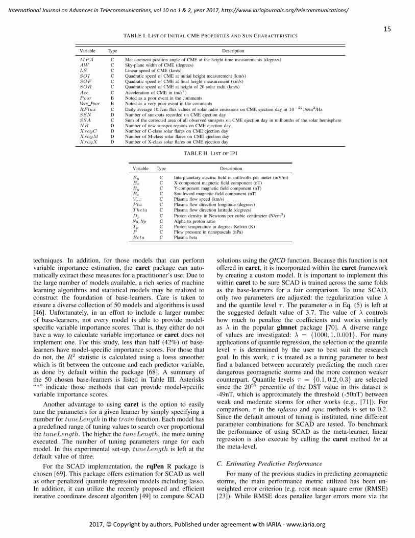
TABLE I. LIST OF INITIAL CME PROPERTIES AND SUN CHARACTERISTICS

Variable Type Description

MPA C Measurement position angle of CME at the height-time measurements (degrees)AW C Sky-plane width of CME (degrees)LS C Linear speed of CME (km/s)SOI C Quadratic speed of CME at initial height measurement (km/s)SOF C Quadratic speed of CME at final height measurement (km/s)SOR C Quadratic speed of CME at height of 20 solar radii (km/s)Acc C Acceleration of CME in (m/s2)Poor B Noted as a poor event in the commentsVery Poor B Noted as a very poor event in the commentsRFlux C Daily average 10.7cm flux values of solar radio emissions on CME ejection day in 10−22J/s/m2/HzSSN D Number of sunspots recorded on CME ejection daySSA C Sum of the corrected area of all observed sunspots on CME ejection day in millionths of the solar hemisphereNR D Number of new sunspot regions on CME ejection dayXrayC D Number of C-class solar flares on CME ejection dayXrayM D Number of M-class solar flares on CME ejection dayXrayX D Number of X-class solar flares on CME ejection day

TABLE II. LIST OF IPI

Variable Type Description

Ey C Interplanetary electric field in millivolts per meter (mV/m)Bx C X-component magnetic field component (nT)By C Y-component magnetic field component (nT)Bz C Southward magnetic field component (nT)Vsw C Plasma flow speed (km/s)Phi C Plasma flow direction longitude (degrees)Theta C Plasma flow direction latitude (degrees)Dp C Proton density in Newtons per cubic centimeter (N/cm3)Na Np C Alpha to proton ratioTp C Proton temperature in degrees Kelvin (K)P C Flow pressure in nanopascals (nPa)Beta C Plasma beta

techniques. In addition, for those models that can performvariable importance estimation, the caret package can auto-matically extract these measures for a practitioner’s use. Due tothe large number of models available, a rich series of machinelearning algorithms and statistical models may be realized toconstruct the foundation of base-learners. Care is taken toensure a diverse collection of 50 models and algorithms is used[46]. Unfortunately, in an effort to include a larger numberof base-learners, not every model is able to provide model-specific variable importance scores. That is, they either do nothave a way to calculate variable importance or caret does notimplement one. For this study, less than half (42%) of base-learners have model-specific importance scores. For those thatdo not, the R2 statistic is calculated using a loess smootherwhich is fit between the outcome and each predictor variable,as done by default within the package [68]. A summary ofthe 50 chosen base-learners is listed in Table III. Asterisks“*” indicate those methods that can provide model-specificvariable importance scores.

Another advantage to using caret is the option to easilytune the parameters for a given learner by simply specifying anumber for tuneLength in the train function. Each model hasa predefined range of tuning values to search over proportionalthe tuneLength. The higher the tuneLength, the more tuningexecuted. The number of tuning parameters range for eachmodel. In this experimental set-up, tuneLength is left at thedefault value of three.

For the SCAD implementation, the rqPen R package ischosen [69]. This package offers estimation for SCAD as wellas other penalized quantile regression models including lasso.In addition, it can utilize the recently proposed and efficientiterative coordinate descent algorithm [49] to compute SCAD

solutions using the QICD function. Because this function is notoffered in caret, it is incorporated within the caret frameworkby creating a custom model. It is important to implement thiswithin caret to be sure SCAD is trained across the same foldsas the base-learners for a fair comparison. To tune SCAD,only two parameters are adjusted: the regularization value λand the quantile level τ . The parameter a in Eq. (5) is left atthe suggested default value of 3.7. The value of λ controlshow much to penalize the coefficients and works similarlyas λ in the popular glmnet package [70]. A diverse rangeof values are investigated: λ = {1000, 1, 0.001}. For manyapplications of quantile regression, the selection of the quantilelevel τ is determined by the user to best suit the researchgoal. In this work, τ is treated as a tuning parameter to bestfind a balanced between accurately predicting the much rarerdangerous geomagnetic storms and the more common weakercounterpart. Quantile levels τ = {0.1, 0.2, 0.3} are selectedsince the 20th percentile of the DST value in this dataset is-49nT, which is approximately the threshold (-50nT) betweenweak and moderate storms for other works (e.g., [71]). Forcomparison, τ in the rqlasso and rqnc methods is set to 0.2.Since the default amount of tuning is instituted, nine differentparameter combinations for SCAD are tested. To benchmarkthe performance of using SCAD as the meta-learner, linearregression is also execute by calling the caret method lm atthe meta-level.

C. Estimating Predictive Performance

For many of the previous studies in predicting geomagneticstorms, the main performance metric utilized has been un-weighted error criterion (e.g. root mean square error (RMSE)[23]). While RMSE does penalize larger errors more via the

15



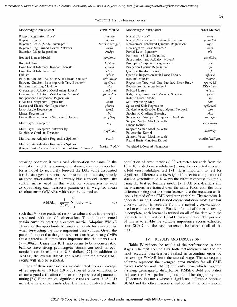
TABLE III. LIST OF BASE-LEARNERS

Model/Algorithm/Learner caret Method Model/Algorithm/Learner caret Method

Bagged Regression Trees* treebag Neural Network* nnetBayesian Lasso blasso Neural Network with Feature Extraction pcaNNetBayesian Lasso (Model Averaged) blassoAveraged Non-convex Penalized Quantile Regression rqncBayesian Regularized Neural Network brnn Non-negative Least Squares* nnlsBayesian Ridge Regression bridge Partial Least Squares* pls

Boosted Linear Model* glmboost Partitioning Using Deletion,Substitution, and Addition Moves* partDSA

Boosted Tree bstTree Principal Component Regression pcrConditional Inference Random Forest* cforest Projection Pursuit Regression pprConditional Inference Tree ctree Quantile Random Forest qrfCubist* cubist Quantile Regression with Lasso Penalty rqlassoExtreme Gradient Boosting with Linear Booster* xgbLinear Random Forest* rangerExtreme Gradient Boosting with Tree Booster* xgbTree Regression Tree with One Standard Error Rule* rpart1SEExtreme Learning Machine elm Regularized Random Forest* RRFglobalGeneralized Additive Model using Loess* gamLoess Relaxed Lasso relaxoGeneralized Additive Model using Splines* gamSpline Ridge Regression with Variable Selection fobaIndependent Component Regression icr Robust Linear Model rlmk-Nearest Neighbors Regression kknn Self-organizing Map bdkLasso and Elastic Net Regression* glmnet Spike and Slab Regression spikeslabLeast Angle Regression lars2 Stacked AutoEncoder Deep Neural Network dnnLinear Regression* lm Stochastic Gradient Boosting* gbmLinear Regression with Stepwise Selection leapSeq Supervised Principal Component Analysis superpc

Multi-layer Perceptron mlp Support Vector Machine withLinear Kernel svmLinear

Multi-layer Perceptron Network byStochastic Gradient Descent* mlpSGD Support Vector Machine with

Polynomial Kernel svmPoly

Multivariate Adaptive Regression Splines* earth Support Vector Machine withRadial Basis Function Kernel svmRadialSigma

Multivariate Adaptive Regression Splines(Bagged with Generalized Cross-validation Pruning)* bagEarthGCV Weighted k-Nearest Neighbors knn

squaring operator, it treats each observation the same. In thecontext of predicting geomagnetic storms, it is more importantfor a model to accurately forecast the DST value associatedfor the strongest of storms. At the same time, focusing strictlyon these observations can severely bias a model. Hence, thecentral metric used in this work for comparison as wellas optimizing each learner’s parameters is weighted meanabsolute error (WMAE), which can be defined as

WMAE =1∑wi

n∑i=1

wi|yi − yi| (6)

such that yi is the predicted response value and wi is the weightassociated with the ith observation. This is implementedwithin caret by creating a custom metric. Adopting WMAEallows for the opportunity to penalize models for inaccuracieswhen forecasting the more important observations. Given thepotential impact that dangerous storms can have, strong CMEsare weighted as 10 times more important than the others (DST> −100nT). Using this 10:1 ratio seems to be a conservativebalance since strong geomangetic storms can result in eco-nomic losses in trillions of U.S. dollars [72]. In addition toWMAE, the overall RMSE and RMSE for the strong CMEevents will also be reported.

Each of these error metrics are calculated from an averageof ten repeats of 10-fold (10 × 10) nested cross-validation toensure a good estimation of error in the presence of parametertuning [73]. Furthermore, significance tests between the SCADmeta-learner and each individual learner are conducted on the

population of error metrics (100 estimates for each from the10 × 10 nested cross-validation) using the corrected repeatedk-fold cross-validation test [74]. It is important to test forsignificant differences to investigate if the extra computation ofstacked generalization is worth the effort compared to simplyusing the best performing model [75]. All base-learners andmeta-learners are trained over the same folds with the onlydifference being that the meta-learners use the metadata as itsinputs instead of the CME predictor variables. The metadata isgenerated using 10-fold nested cross-validation. Note that thiscross-validation is separate from the nested cross-validationused to estimate the error. Finally, after all of the error testingis complete, each learner is trained on all of the data with theparameters optimized via 10-fold cross-validation. The purposeof this is to enable the variable importance scores extractedfrom SCAD and the base-learners to be based on all of thedata.

IV. RESULTS AND DISCUSSION

Table IV reflects the results of the performance in bothstages. The first column lists both meta-learners and the tenmost accurate base-learners ranked in ascending order bythe average WMAE from the second stage. The subsequentcolumns represent the averaged error metrics for all CMEevents (WMAE and RMSE) and only those which triggereda strong geomagnetic disturbance (RMSE). Bold and italicsindicate the best performing method. The dagger symbol“†” denotes instances where a significant difference betweenSCAD and the other learners is not found at the conventional

16



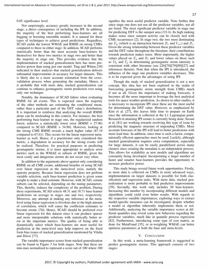
0.05 significance level.Not surprisingly, accuracy greatly increases in the second

stage, a direct consequence of including the IPI. In addition,the majority of the best performing base-learners are allbagging or boosting ensemble models. It is natural for thesetypes of techniques to achieve good predictions. Regardless,SCAD yields the lowest WMAE and RMSE on strong CMEscompared to these in either stage. In addition, SCAD performsstatistically better than the most accurate base-learners bythemselves for these two metrics in stage two and better thanthe majority in stage one. This provides evidence that theimplementation of stacked generalization here has more pre-dictive power than using just one model. Ting and Witten [39]indicated in their analysis that stacked generalization deliverssubstantial improvements in accuracy for larger datasets. Thisis likely due to a more accurate estimation from the cross-validation process when generating the metadata. Hence, itis probable that with more data, stacked generalization cancontinue to enhance geomagnetic storm prediction over usingonly one technique.

Notably, the dominance of SCAD falters when evaluatingRMSE for all events. This is expected since the majorityof the other methods are estimating the conditional mean,rather than a particular part of the DST value’s distribution.It is important to reinforce that analyzing the overall RMSEalone can be misleading in this context. For instance, the bestperforming base-learner in stage one, the regularized randomforest, achieves a statistically lower error (RMSE = 27.96)compared to SCAD (RMSE = 34.90). However, looking atthe strong CME RMSE reveals a much higher value (87.19compared to 67.61). This occurs for the linear regression meta-learner as well. Hence, if a practitioner only considered thismetric, a degradation in accuracy for the strong events willbe realized. Therefore, for practical purposes in predictinggeomagnetic storms, it is more appropriate to analyze errormetrics such as the WMAE or subsets of RMSE, given themost costly and dangerous storms do not occur very often.

In addition to the arguments above against only consideringRMSE on all CME events, additional benefits of using SCADover linear regression at the meta-level exist, namely thesparsity property. Because linear regression does not performvariable selection, each base-learner prediction is given someweight to make a final estimate. However, with SCAD, certainsubsets can be selected, depending on the tuning parameters.This, thereby, reduces the complexity of the problem. Duringthese experiments, SCAD selects 48.31 and 18.71 base-learnerpredictions on average in stages one and two, respectively.Moreover, any attempt at making any inference at the meta-level using linear regression is frivolous due to the high amountof correlation, which will cause the coefficient estimates tobecome erratic [76]. Hence, SCAD should be preferred overlinear regression for this dataset since it can produce sparserand more interpretable solutions with statistically better er-ror in the important metrics. The quality of being able todynamically select which base-learners are most useful forprediction at the meta-level may help improve on the fixedform bias issues of stacked generalization mentioned by Vilaltaand Drissi [77].

The variable importance scores from stacked generalizationcan be found in Figure 3 for both stages. Note that these aremin-max normalized to represent a score out of 100 where 100

signifies the most useful predictor variable. Note further thatsince stage one does not use all the predictor variables, not allare listed. The most significant predictor variable in stage onefor predicting DST is the sunspot area (SSA). Its high rankingmakes sense since sunspot activity can be closely tied withCME occurrences [2]. In stage two, the two most dominatingare Ey (which is an interaction between Bz and Vsw) and Bz .Given the strong relationship between these predictor variablesand the DST value throughout the literature, their contributionstowards prediction makes sense. More importantly, the highervalues placed on Ey and Bz and lower values on those suchas Dp and Tp in determining geomagnetic storm intensity isconsistent with other literature (see [26][78][79][80][27] andreferences therein). Note that when the IPI is introduced, theinfluence of the stage one predictor variables decreases. Thisis to be expected given the advantages of using IPI.

Though the study of stacked generalization is not a newconcept, this idea has not been explored in the realm offorecasting geomagnetic storm strength from CMEs muchif not at all. Given the importance of making forecasts, itbecomes all the more important to leverage the best analyticaltools for space weather prediction. As shown in other studies, itis necessary to incorporate IPI since these are the most usefulfor determining the DST value. However, as emphasized byKim et al. [27], this leaves little time to prepare on Earthonce the information is collected at the L1 Lagrangian point.Research in attaining IPI sooner is currently being done. Savaniet al. [81] are working towards resolving this type of issue bypredicting the magnetic structure of impending CMEs. Moreaccurate forecasts of the IPI will lead to better predictions withmore lead time. In addition, since time is such a factor, compu-tationally efficient approaches must be used. Luckily, althoughstacked generalization requires extra computation, especiallyfor large datasets, it can be easily parallelized across manyclusters since creating the metadata is an independent process.This allows for scalability as new models and algorithms areconstantly being developed. Incorporating a larger number offaster and smarter base-learners provides the opportunity toincrease predictive power.

This study brings several future work opportunities. Firstly,as more data is collected on CMEs in more advanced ways,implementation on larger datasets is possible for both clas-sification and regression tasks. With more data, stacked gen-eralization is more probable to find predictive improvements[39]. Secondly, this work only includes 50 base-learners.Increasing this number by incorporating different models andalgorithms could yield even better results. With regards tothe respective variable importances, exploring ways to extractmodel-specific measures can be investigated, despite whethera model or algorithm inherently implements them or not.Additionally, analyzing the variable importance scores at dif-ferent quantiles may reveal some new behaviors regarding thepredictor variables, much like in quantile process regression[82]. Furthermore, introducing some type of cost matrix, asdone for MetaFraud [35], or re-weighting WMAE can betteroptimize parameters at both the base and meta-levels.

V. CONCLUSION

In this work, a meta-learning framework is suggested topredict geomagnetic storms. This approach consists of twostages:

17



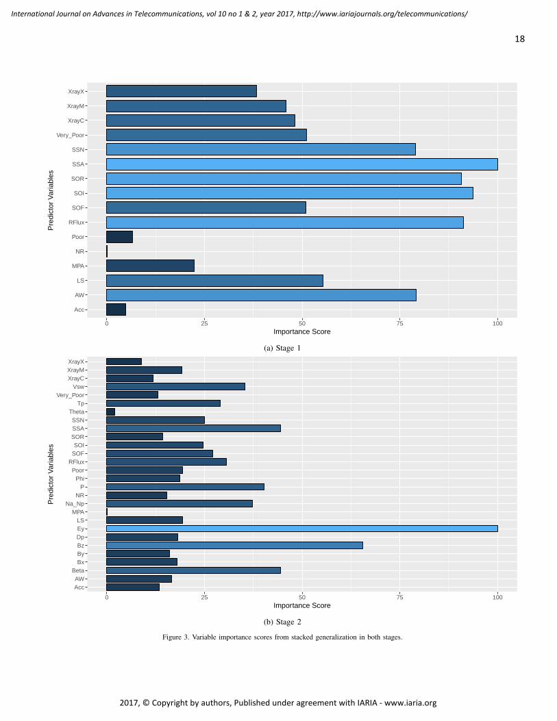
Acc

AW

LS

MPA

NR

Poor

RFlux

SOF

SOI

SOR

SSA

SSN

Very_Poor

XrayC

XrayM

XrayX

0 25 50 75 100Importance Score

Pre

dict

or V

aria

bles

(a) Stage 1

AccAW

BetaBxByBzDpEyLS

MPANa_Np

NRP

PhiPoor

RFluxSOFSOI

SORSSASSN

ThetaTp

Very_PoorVsw

XrayCXrayMXrayX

0 25 50 75 100Importance Score

Pre

dict

or V

aria

bles

(b) Stage 2

Figure 3. Variable importance scores from stacked generalization in both stages.

18



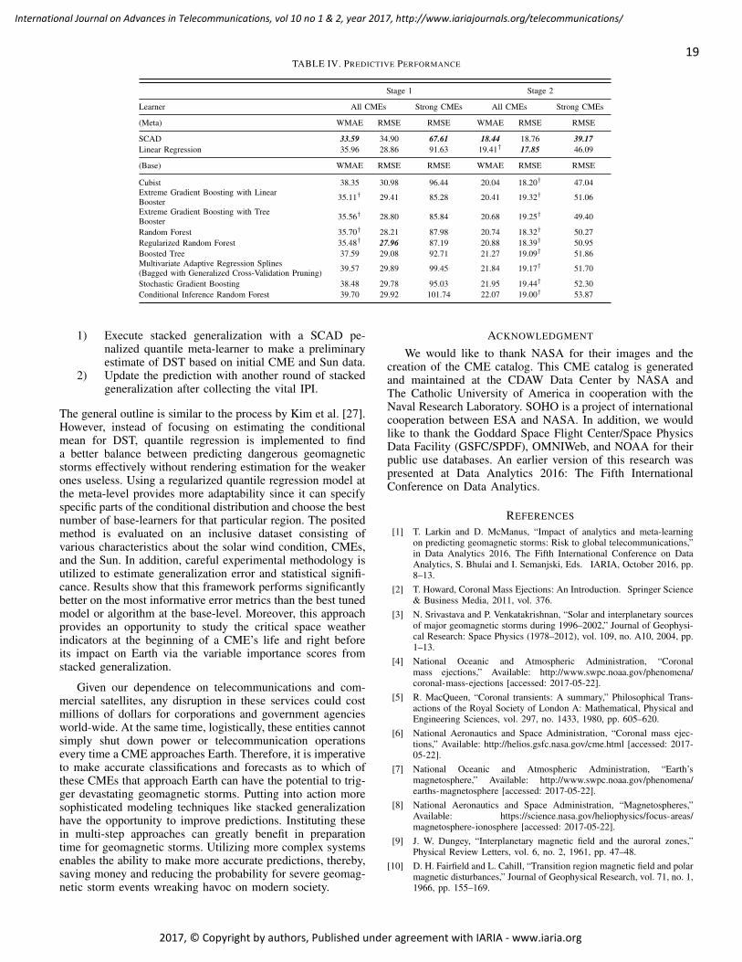
TABLE IV. PREDICTIVE PERFORMANCE

Stage 1 Stage 2

Learner All CMEs Strong CMEs All CMEs Strong CMEs

(Meta) WMAE RMSE RMSE WMAE RMSE RMSE

SCAD 33.59 34.90 67.61 18.44 18.76 39.17Linear Regression 35.96 28.86 91.63 19.41† 17.85 46.09

(Base) WMAE RMSE RMSE WMAE RMSE RMSE

Cubist 38.35 30.98 96.44 20.04 18.20† 47.04Extreme Gradient Boosting with LinearBooster 35.11† 29.41 85.28 20.41 19.32† 51.06

Extreme Gradient Boosting with TreeBooster 35.56† 28.80 85.84 20.68 19.25† 49.40

Random Forest 35.70† 28.21 87.98 20.74 18.32† 50.27Regularized Random Forest 35.48† 27.96 87.19 20.88 18.39† 50.95Boosted Tree 37.59 29.08 92.71 21.27 19.09† 51.86Multivariate Adaptive Regression Splines(Bagged with Generalized Cross-Validation Pruning) 39.57 29.89 99.45 21.84 19.17† 51.70

Stochastic Gradient Boosting 38.48 29.78 95.03 21.95 19.44† 52.30Conditional Inference Random Forest 39.70 29.92 101.74 22.07 19.00† 53.87

1) Execute stacked generalization with a SCAD pe-nalized quantile meta-learner to make a preliminaryestimate of DST based on initial CME and Sun data.

2) Update the prediction with another round of stackedgeneralization after collecting the vital IPI.

The general outline is similar to the process by Kim et al. [27].However, instead of focusing on estimating the conditionalmean for DST, quantile regression is implemented to finda better balance between predicting dangerous geomagneticstorms effectively without rendering estimation for the weakerones useless. Using a regularized quantile regression model atthe meta-level provides more adaptability since it can specifyspecific parts of the conditional distribution and choose the bestnumber of base-learners for that particular region. The positedmethod is evaluated on an inclusive dataset consisting ofvarious characteristics about the solar wind condition, CMEs,and the Sun. In addition, careful experimental methodology isutilized to estimate generalization error and statistical signifi-cance. Results show that this framework performs significantlybetter on the most informative error metrics than the best tunedmodel or algorithm at the base-level. Moreover, this approachprovides an opportunity to study the critical space weatherindicators at the beginning of a CME’s life and right beforeits impact on Earth via the variable importance scores fromstacked generalization.

Given our dependence on telecommunications and com-mercial satellites, any disruption in these services could costmillions of dollars for corporations and government agenciesworld-wide. At the same time, logistically, these entities cannotsimply shut down power or telecommunication operationsevery time a CME approaches Earth. Therefore, it is imperativeto make accurate classifications and forecasts as to which ofthese CMEs that approach Earth can have the potential to trig-ger devastating geomagnetic storms. Putting into action moresophisticated modeling techniques like stacked generalizationhave the opportunity to improve predictions. Instituting thesein multi-step approaches can greatly benefit in preparationtime for geomagnetic storms. Utilizing more complex systemsenables the ability to make more accurate predictions, thereby,saving money and reducing the probability for severe geomag-netic storm events wreaking havoc on modern society.

ACKNOWLEDGMENT

We would like to thank NASA for their images and thecreation of the CME catalog. This CME catalog is generatedand maintained at the CDAW Data Center by NASA andThe Catholic University of America in cooperation with theNaval Research Laboratory. SOHO is a project of internationalcooperation between ESA and NASA. In addition, we wouldlike to thank the Goddard Space Flight Center/Space PhysicsData Facility (GSFC/SPDF), OMNIWeb, and NOAA for theirpublic use databases. An earlier version of this research waspresented at Data Analytics 2016: The Fifth InternationalConference on Data Analytics.

REFERENCES

[1] T. Larkin and D. McManus, “Impact of analytics and meta-learningon predicting geomagnetic storms: Risk to global telecommunications,”in Data Analytics 2016, The Fifth International Conference on DataAnalytics, S. Bhulai and I. Semanjski, Eds. IARIA, October 2016, pp.8–13.

[2] T. Howard, Coronal Mass Ejections: An Introduction. Springer Science& Business Media, 2011, vol. 376.

[3] N. Srivastava and P. Venkatakrishnan, “Solar and interplanetary sourcesof major geomagnetic storms during 1996–2002,” Journal of Geophysi-cal Research: Space Physics (1978–2012), vol. 109, no. A10, 2004, pp.1–13.

[4] National Oceanic and Atmospheric Administration, “Coronalmass ejections,” Available: http://www.swpc.noaa.gov/phenomena/coronal-mass-ejections [accessed: 2017-05-22].

[5] R. MacQueen, “Coronal transients: A summary,” Philosophical Trans-actions of the Royal Society of London A: Mathematical, Physical andEngineering Sciences, vol. 297, no. 1433, 1980, pp. 605–620.

[6] National Aeronautics and Space Administration, “Coronal mass ejec-tions,” Available: http://helios.gsfc.nasa.gov/cme.html [accessed: 2017-05-22].

[7] National Oceanic and Atmospheric Administration, “Earth’smagnetosphere,” Available: http://www.swpc.noaa.gov/phenomena/earths-magnetosphere [accessed: 2017-05-22].

[8] National Aeronautics and Space Administration, “Magnetospheres,”Available: https://science.nasa.gov/heliophysics/focus-areas/magnetosphere-ionosphere [accessed: 2017-05-22].

[9] J. W. Dungey, “Interplanetary magnetic field and the auroral zones,”Physical Review Letters, vol. 6, no. 2, 1961, pp. 47–48.

[10] D. H. Fairfield and L. Cahill, “Transition region magnetic field and polarmagnetic disturbances,” Journal of Geophysical Research, vol. 71, no. 1,1966, pp. 155–169.

19



[11] W. D. Gonzalez and B. T. Tsurutani, “Criteria of interplanetary param-eters causing intense magnetic storms (DST <-100 nT),” Planetary andSpace Science, vol. 35, no. 9, 1987, pp. 1101–1109.

[12] Y. Wang, P. Ye, S. Wang, G. Zhou, and J. Wang, “A statistical studyon the geoeffectiveness of Earth-directed coronal mass ejections fromMarch 1997 to December 2000,” Journal of Geophysical Research:Space Physics (1978–2012), vol. 107, no. A11, 2002, pp. SSH 2–1–SSH 2–9.

[13] J. Kappernman and V. D. Albertson, “Bracing for the geomagneticstorms,” Spectrum, IEEE, vol. 27, no. 3, 1990, pp. 27–33.

[14] Space Studies Board and others, Severe Space Weather Events: Un-derstanding Societal and Economic Impacts: A Workshop Report.National Academies Press, 2008.

[15] D. Baker, X. Li, A. Pulkkinen, C. Ngwira, M. Mays, A. Galvin, andK. Simunac, “A major solar eruptive event in July 2012: Definingextreme space weather scenarios,” Space Weather, vol. 11, no. 10, 2013,pp. 585–591.

[16] J. Gosling, S. Bame, D. McComas, and J. Phillips, “Coronal massejections and large geomagnetic storms,” Geophysical Research Letters,vol. 17, no. 7, 1990, pp. 901–904.

[17] V. Bothmer and R. Schwenn, “The interplanetary and solar causes ofmajor geomagnetic storms,” Journal of Geomagnetism and Geoelectric-ity, vol. 47, no. 11, 1995, pp. 1127–1132.

[18] B. T. Tsurutani and W. D. Gonzalez, “The interplanetary causes ofmagnetic storms: A review,” Washington DC American GeophysicalUnion Geophysical Monograph Series, vol. 98, 1997, pp. 77–89.

[19] J. Zhang, K. Dere, R. Howard, and V. Bothmer, “Identification of solarsources of major geomagnetic storms between 1996 and 2000,” TheAstrophysical Journal, vol. 582, no. 1, 2003, pp. 520–533.

[20] D. McManus, H. Carr, and B. Adams, “Wireless on the precipice: The14th century revisited,” Communications of the ACM, vol. 54, no. 6,2011, pp. 138–143.

[21] R. K. Burton, R. McPherron, and C. Russell, “An empirical relationshipbetween interplanetary conditions and DST,” Journal of GeophysicalResearch, vol. 80, no. 31, 1975, pp. 4204–4214.

[22] M. Sugiura, “Hourly values of equatorial DST for the IGY,” Ann. Int.Geophys. Yr., vol. 35, 1964, pp. 1–44.

[23] E.-Y. Ji, Y.-J. Moon, N. Gopalswamy, and D.-H. Lee, “Comparisonof DST forecast models for intense geomagnetic storms,” Journal ofGeophysical Research: Space Physics, vol. 117, no. A3, 2012, pp. 1–9.

[24] T. Andriyas and S. Andriyas, “Relevance vector machines as a tool forforecasting geomagnetic storms during years 1996–2007,” Journal ofAtmospheric and Solar-Terrestrial Physics, vol. 125, 2015, pp. 10–20.

[25] M. Dryer, Z. Smith, C. Fry, W. Sun, C. Deehr, and S.-I. Akasofu, “Real-time shock arrival predictions during the halloween 2003 epoch,” SpaceWeather, vol. 2, no. 9, 2004, pp. 1–10.

[26] N. Srivastava, “A logistic regression model for predicting the occurrenceof intense geomagnetic storms,” in Annales Geophysicae, vol. 23, no. 9,2005, pp. 2969–2974.

[27] R.-S. Kim, Y.-J. Moon, N. Gopalswamy, Y.-D. Park, and Y.-H. Kim,“Two-step forecast of geomagnetic storm using coronal mass ejectionand solar wind condition,” Space Weather, vol. 12, no. 4, 2014, pp.246–256.

[28] J. Uwamahoro, L. McKinnell, and J. Habarulema, “Estimating thegeoeffectiveness of halo CMEs from associated solar and IP parametersusing neural networks,” Annales Geophysicae-Atmospheres Hydro-spheresand Space Sciences, vol. 30, no. 6, 2012, pp. 963–972.

[29] F. Valach, J. Bochnıcek, P. Hejda, and M. Revallo, “Strong geomagneticactivity forecast by neural networks under dominant southern orienta-tion of the interplanetary magnetic field,” Advances in Space Research,vol. 53, no. 4, 2014, pp. 589–598.

[30] R. Schwenn, “Space weather: The solar perspective,” Living Reviewsin Solar Physics, vol. 3, no. 1, 2006, pp. 1–72.

[31] V. Yurchyshyn, V. Abramenko, and D. Tripathi, “Rotation of white-lightcoronal mass ejection structures as inferred from lasco coronagraph,”The Astrophysical Journal, vol. 705, no. 1, 2009, p. 426.

[32] D. M. Hawkins, “The problem of overfitting,” Journal of ChemicalInformation and Computer Sciences, vol. 44, no. 1, 2004, pp. 1–12.

[33] T. Larkin, “Advanced analytical tools for geomagnetic storm prediction:Ensembles and their insights,” Ph.D. dissertation, The University ofAlabama, 2017, unpublished thesis.

[34] D. H. Wolpert, “Stacked generalization,” Neural Networks, vol. 5, no. 2,1992, pp. 241–259.

[35] A. Abbasi, C. Albrecht, A. Vance, and J. Hansen, “Metafraud: Ameta-learning framework for detecting financial fraud,” MIS Quarterly,vol. 36, no. 4, 2012, pp. 1293–1327.

[36] C.-F. Tsai and Y.-F. Hsu, “A meta-learning framework for bankruptcyprediction,” Journal of Forecasting, vol. 32, no. 2, 2013, pp. 167–179.

[37] J. Sill, G. Takacs, L. Mackey, and D. Lin, “Feature-weighted linearstacking,” arXiv preprint arXiv:0911.0460, 2009, pp. 1–17.

[38] L. Breiman, “Stacked regressions,” Machine Learning, vol. 24, no. 1,1996, pp. 49–64.

[39] K. M. Ting and I. H. Witten, “Issues in stacked generalization,” J. Artif.Intell. Res.(JAIR), vol. 10, 1999, pp. 271–289.

[40] R. Caruana, A. Niculescu-Mizil, G. Crew, and A. Ksikes, “Ensembleselection from libraries of models,” in Proceedings of the Twenty-firstInternational Conference on Machine Learning. ACM, 2004, pp. 18–25.

[41] M. LeBlanc and R. Tibshirani, “Combining estimates in regression andclassification,” Journal of the American Statistical Association, vol. 91,no. 436, 1996, pp. 1641–1650.

[42] S. Reid and G. Grudic, “Regularized linear models in stacked general-ization,” in Multiple Classifier Systems. Springer, 2009, pp. 112–121.

[43] A. E. Hoerl and R. W. Kennard, “Ridge regression: Biased estimationfor nonorthogonal problems,” Technometrics, 1970, pp. 55–67.

[44] R. Tibshirani, “Regression shrinkage and selection via the lasso,”Journal of the Royal Statistical Society. Series B (Methodological),1996, pp. 267–288.

[45] H. Zou and T. Hastie, “Regularization and variable selection via theelastic net,” Journal of the Royal Statistical Society: Series B (StatisticalMethodology), vol. 67, no. 2, 2005, pp. 301–320.

[46] G. Zenobi and P. Cunningham, “Using diversity in preparing ensemblesof classifiers based on different feature subsets to minimize generaliza-tion error,” in Machine Learning: ECML 2001. Springer, 2001, pp.576–587.

[47] Z.-H. Zhou, J. Wu, and W. Tang, “Ensembling neural networks: manycould be better than all,” Artificial Intelligence, vol. 137, no. 1, 2002,pp. 239–263.

[48] N. Rooney, D. Patterson, and C. Nugent, “Pruning extensions tostacking,” Intelligent Data Analysis, vol. 10, no. 1, 2006, pp. 47–66.

[49] B. Peng and L. Wang, “An iterative coordinate descent algorithm forhigh-dimensional nonconvex penalized quantile regression,” Journal ofComputational and Graphical Statistics, vol. 24, no. 3, 2015, pp. 676–694.

[50] F. Mosteller and J. W. Tukey, “Data analysis and regression: A secondcourse in statistics,” Addison-Wesley Series in Behavioral Science:Quantitative Methods, 1977.

[51] B. S. Cade and B. R. Noon, “A gentle introduction to quantile regressionfor ecologists,” Frontiers in Ecology and the Environment, vol. 1, no. 8,2003, pp. 412–420.

[52] R. Koenker and G. Bassett Jr, “Regression quantiles,” Econometrica:Journal of the Econometric Society, 1978, pp. 33–50.

[53] R. Koenker and K. Hallock, “Quantile regression: An introduction,”Journal of Economic Perspectives, vol. 15, no. 4, 2001, pp. 43–56.

[54] R. Koenker, “Quantile regression for longitudinal data,” Journal ofMultivariate Analysis, vol. 91, no. 1, 2004, pp. 74–89.

[55] Y. Li and J. Zhu, “L1-norm quantile regression,” Journal of Computa-tional and Graphical Statistics, 2012.

[56] J. Fan and R. Li, “Variable selection via nonconcave penalized like-lihood and its oracle properties,” Journal of the American StatisticalAssociation, vol. 96, no. 456, 2001, pp. 1348–1360.

[57] H. Zou, “The adaptive lasso and its oracle properties,” Journal of theAmerican Statistical Association, vol. 101, no. 476, 2006, pp. 1418–1429.

[58] F. Audrino and L. Camponovo, “Oracle properties and finite sample

20



inference of the adaptive lasso for time series regression models,” arXivpreprint arXiv:1312.1473, 2013.

[59] Y. Wu and Y. Liu, “Variable selection in quantile regression,” StatisticaSinica, 2009, pp. 801–817.

[60] H. Cane and I. Richardson, “Interplanetary coronal mass ejections inthe near-earth solar wind during 1996–2002,” Journal of GeophysicalResearch: Space Physics (1978–2012), vol. 108, no. A4, 2003, pp. SSH6–1–SSH 6–13.

[61] I. Richardson and H. Cane, “Near-earth interplanetary coronal massejections during solar cycle 23 (1996–2009): Catalog and summary ofproperties,” Solar Physics, vol. 264, no. 1, 2010, pp. 189–237.

[62] J. King and N. Papitashvili, “Solar wind spatial scales in and compar-isons of hourly wind and ACE plasma and magnetic field data,” Journalof Geophysical Research: Space Physics, vol. 110, no. A2, 2005, pp.1–8.

[63] N. Gopalswamy, S. Yashiro, G. Michalek, G. Stenborg, A. Vourlidas,S. Freeland, and R. Howard, “The SOHO/LASCO CME catalog,” Earth,Moon, and Planets, vol. 104, no. 1-4, 2009, pp. 295–313.

[64] National Oceanic and Atmospheric Administration, “Index of/pub/warehouse,” Available: ftp://ftp.swpc.noaa.gov/pub/warehouse [ac-cessed: 2017-05-22].

[65] G.-H. Moon, “Variation of Magnetic Field (By, Bz) Polarity andStatistical Analysis of Solar Wind Parameters during the MagneticStorm Period,” Journal of Astronomy and Space Sciences, vol. 28, no. 2,2011, pp. 123–132.

[66] R Core Team, R: A Language and Environment for Statistical Com-puting, R Foundation for Statistical Computing, Vienna, Austria, 2017,Available: https://www.R-project.org/ [accessed: 2017-05-22].

[67] M. K. C. from Jed Wing, S. Weston, A. Williams, C. Keefer, A. En-gelhardt, T. Cooper, Z. Mayer, B. Kenkel, the R Core Team, M. Ben-esty, R. Lescarbeau, A. Ziem, L. Scrucca, Y. Tang, C. Candan, andT. Hunt., caret: classification and regression training, 2016, R packageversion 6.0-70. Available: https://CRAN.R-project.org/package=caret[accessed: 2016-07-27].

[68] M. Kuhn, “Building predictive models in R using the caret package,”Journal of Statistical Software, vol. 28, no. 5, 2008, pp. 1–26.

[69] B. Sherwood and A. Maidman, rqPen: Penalized Quantile Regression,2016, R package version 1.4. Available: https://CRAN.R-project.org/package=rqPen [accessed: 2016-07-27].

[70] J. Friedman, T. Hastie, and R. Tibshirani, “Regularization paths forgeneralized linear models via coordinate descent,” Journal of StatisticalSoftware, vol. 33, no. 1, 2010, p. 1.

[71] C. Loewe and G. Prolss, “Classification and mean behavior of magneticstorms,” Journal of Geophysical Research: Space Physics, vol. 102,no. A7, 1997, pp. 14 209–14 213.

[72] Lloyd’s and the Atmospheric and Environmental Research Inc.,“Solar storm risk to the north american electrical grid,” 2013,Available: https://www.lloyds.com/∼/media/lloyds/reports/emerging%20risk%20reports/solar%20storm%20risk%20to%20the%20north%20american%20electric%20grid.pdf [accessed: 2017-05-22].

[73] S. Varma and R. Simon, “Bias in error estimation when using cross-validation for model selection,” BMC Bioinformatics, vol. 7, no. 1,2006, p. 91.

[74] R. R. Bouckaert and E. Frank, “Evaluating the replicability of sig-nificance tests for comparing learning algorithms,” in Advances inKnowledge Discovery and Data Mining. Springer, 2004, pp. 3–12.

[75] S. Dzeroski and B. Zenko, “Is combining classifiers with stacking betterthan selecting the best one?” Machine Learning, vol. 54, no. 3, 2004,pp. 255–273.

[76] T. Hastie, R. Tibshirani, and J. Friedman, The Elements of StatisticalLearning: Data Mining, Inference, and Prediction. New York: Springer,2009.

[77] R. Vilalta and Y. Drissi, “A perspective view and survey of meta-learning,” Artificial Intelligence Review, vol. 18, no. 2, 2002, pp. 77–95.

[78] E. Echer, W. Gonzalez, and B. Tsurutani, “Interplanetary conditionsleading to superintense geomagnetic storms (DST <= -250 nT) duringsolar cycle 23,” Geophysical Research Letters, vol. 35, no. 6, 2008.

[79] Y. I. Yermolaev, M. Y. Yermolaev, I. Lodkina, and N. Nikolaeva,

“Statistical investigation of heliospheric conditions resulting in magneticstorms: 2,” Cosmic Research, vol. 45, no. 6, 2007, pp. 461–470.

[80] E.-Y. Ji, Y.-J. Moon, K.-H. Kim, and D.-H. Lee, “Statistical comparisonof interplanetary conditions causing intense geomagnetic storms (DST<= -100 nT),” Journal of Geophysical Research: Space Physics (1978–2012), vol. 115, no. A10, 2010.

[81] N. Savani, A. Vourlidas, A. Szabo, M. Mays, I. Richardson, B. Thomp-son, A. Pulkkinen, R. Evans, and T. Nieves-Chinchilla, “Predicting themagnetic vectors within coronal mass ejections arriving at earth: 1.initial architecture,” Space Weather, 2015.

[82] R. Koenker and J. A. Machado, “Goodness of fit and related inferenceprocesses for quantile regression,” Journal of the American StatisticalAssociation, vol. 94, no. 448, 1999, pp. 1296–1310.

21



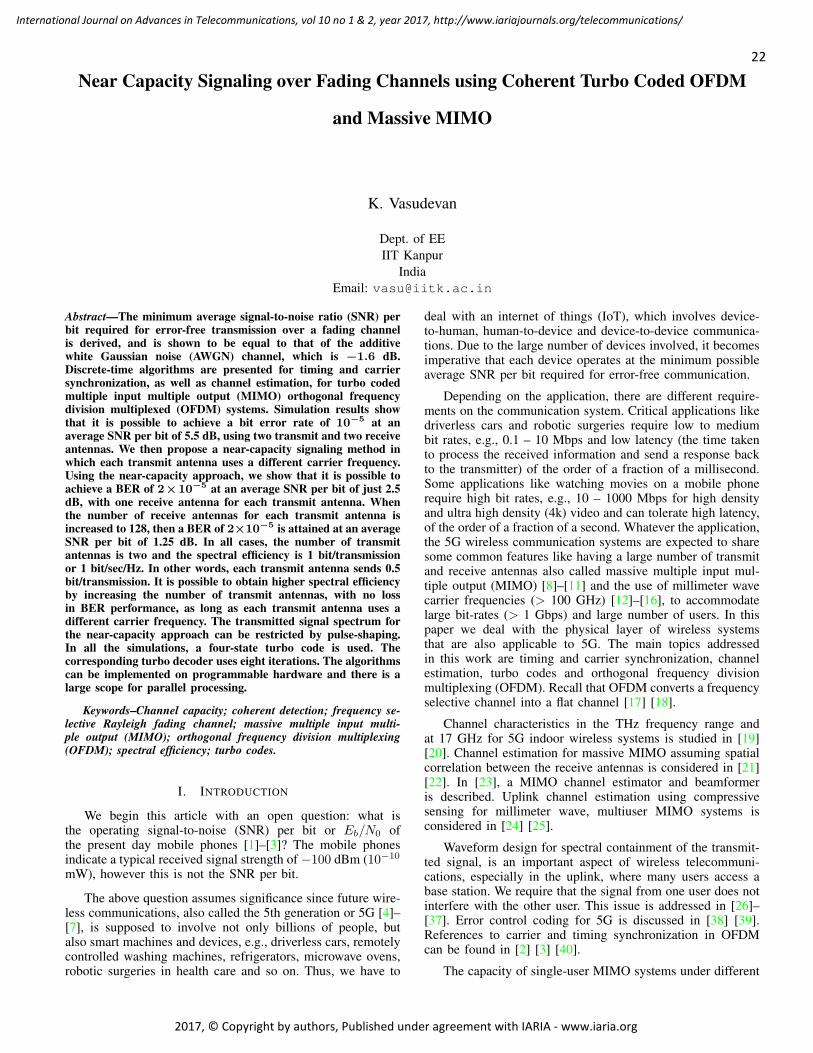
Near Capacity Signaling over Fading Channels using Coherent Turbo Coded OFDM

and Massive MIMO

K. Vasudevan

Dept. of EE

IIT Kanpur

India

Email: [email protected]

Abstract—The minimum average signal-to-noise ratio (SNR) perbit required for error-free transmission over a fading channelis derived, and is shown to be equal to that of the additivewhite Gaussian noise (AWGN) channel, which is −1.6 dB.Discrete-time algorithms are presented for timing and carriersynchronization, as well as channel estimation, for turbo codedmultiple input multiple output (MIMO) orthogonal frequencydivision multiplexed (OFDM) systems. Simulation results showthat it is possible to achieve a bit error rate of 10

−5 at anaverage SNR per bit of 5.5 dB, using two transmit and two receiveantennas. We then propose a near-capacity signaling method inwhich each transmit antenna uses a different carrier frequency.Using the near-capacity approach, we show that it is possible toachieve a BER of 2×10

−5 at an average SNR per bit of just 2.5dB, with one receive antenna for each transmit antenna. Whenthe number of receive antennas for each transmit antenna isincreased to 128, then a BER of 2×10

−5 is attained at an averageSNR per bit of 1.25 dB. In all cases, the number of transmitantennas is two and the spectral efficiency is 1 bit/transmissionor 1 bit/sec/Hz. In other words, each transmit antenna sends 0.5bit/transmission. It is possible to obtain higher spectral efficiencyby increasing the number of transmit antennas, with no lossin BER performance, as long as each transmit antenna uses adifferent carrier frequency. The transmitted signal spectrum forthe near-capacity approach can be restricted by pulse-shaping.In all the simulations, a four-state turbo code is used. Thecorresponding turbo decoder uses eight iterations. The algorithmscan be implemented on programmable hardware and there is alarge scope for parallel processing.

Keywords–Channel capacity; coherent detection; frequency se-lective Rayleigh fading channel; massive multiple input multi-ple output (MIMO); orthogonal frequency division multiplexing(OFDM); spectral efficiency; turbo codes.

I. INTRODUCTION

We begin this article with an open question: what isthe operating signal-to-noise (SNR) per bit or Eb/N0 ofthe present day mobile phones [1]–[3]? The mobile phonesindicate a typical received signal strength of −100 dBm (10−10

mW), however this is not the SNR per bit.

The above question assumes significance since future wire-less communications, also called the 5th generation or 5G [4]–[7], is supposed to involve not only billions of people, butalso smart machines and devices, e.g., driverless cars, remotelycontrolled washing machines, refrigerators, microwave ovens,robotic surgeries in health care and so on. Thus, we have to

deal with an internet of things (IoT), which involves device-to-human, human-to-device and device-to-device communica-tions. Due to the large number of devices involved, it becomesimperative that each device operates at the minimum possibleaverage SNR per bit required for error-free communication.

Depending on the application, there are different require-ments on the communication system. Critical applications likedriverless cars and robotic surgeries require low to mediumbit rates, e.g., 0.1 – 10 Mbps and low latency (the time takento process the received information and send a response backto the transmitter) of the order of a fraction of a millisecond.Some applications like watching movies on a mobile phonerequire high bit rates, e.g., 10 – 1000 Mbps for high densityand ultra high density (4k) video and can tolerate high latency,of the order of a fraction of a second. Whatever the application,the 5G wireless communication systems are expected to sharesome common features like having a large number of transmitand receive antennas also called massive multiple input mul-tiple output (MIMO) [8]–[11] and the use of millimeter wavecarrier frequencies (> 100 GHz) [12]–[16], to accommodatelarge bit-rates (> 1 Gbps) and large number of users. In thispaper we deal with the physical layer of wireless systemsthat are also applicable to 5G. The main topics addressedin this work are timing and carrier synchronization, channelestimation, turbo codes and orthogonal frequency divisionmultiplexing (OFDM). Recall that OFDM converts a frequencyselective channel into a flat channel [17] [18].

Channel characteristics in the THz frequency range andat 17 GHz for 5G indoor wireless systems is studied in [19][20]. Channel estimation for massive MIMO assuming spatialcorrelation between the receive antennas is considered in [21][22]. In [23], a MIMO channel estimator and beamformeris described. Uplink channel estimation using compressivesensing for millimeter wave, multiuser MIMO systems isconsidered in [24] [25].

Waveform design for spectral containment of the transmit-ted signal, is an important aspect of wireless telecommuni-cations, especially in the uplink, where many users access abase station. We require that the signal from one user does notinterfere with the other user. This issue is addressed in [26]–[37]. Error control coding for 5G is discussed in [38] [39].References to carrier and timing synchronization in OFDMcan be found in [2] [3] [40].

The capacity of single-user MIMO systems under different

22



assumptions about the channel impulse response (also calledthe channel state information or CSI) and the statistics ofthe channel impulse response (also called channel distributioninformation or CDI) is discussed in [41]. The capacity ofMIMO Rayleigh fading channels in the presence of interfer-ence and receive correlation is discussed in [42]. The low SNRcapacity of MIMO fading channels with imperfect channelstate information is presented in [43].

The main contribution of this paper is to develop discrete-time algorithms for coherently detecting multiple input, multi-ple output (MIMO), orthogonal frequency division multiplexed(OFDM) signals, transmitted over frequency selective Rayleighfading channels. Carrier frequency offset and additive whiteGaussian noise (AWGN) are the other impairments consideredin this work. The minimum SNR per bit required for error-freetransmission over frequency selective MIMO fading channelsis derived. Finally we demonstrate how we can approach closeto the channel capacity.

To the best of our knowledge, other than the work in[40], which deals with turbo coded single input single output(SISO) OFDM, and [2] [3], which deal with turbo coded singleinput multiple output (SIMO) OFDM, discrete-time algorithmsfor the coherent detection of turbo coded MIMO OFDMsystems have not been discussed earlier in the literature.Coherent detectors for AWGN channels is discussed in [44][45]. Simulations results for a 2×2 turbo coded MIMO OFDMsystem indicate that a BER of 10−5, is obtained at an averageSNR per bit of just 5.5 dB, which is a 2.5 dB improvementover the performance given in [2]. If each transmit antennatransmits at a different carrier frequency, then we show thatit is possible to achieve a BER of 2 × 10−5 at an averageSNR per bit of just 2.5 dB, with one receive antenna for eachtransmit antenna. When the number of receive antennas foreach transmit antenna is increased to 128, then a BER of2×10−5 is obtained at an average SNR per bit of 1.25 dB. In allcases, the number of transmit antennas is two and the spectralefficiency is 1 bit/transmission or 1 bit/sec/Hz. In other words,each transmit antenna sends 0.5 bit/transmission. It is possibleto obtain higher spectral efficiency by increasing the number oftransmit antennas, with no loss in BER performance, as longas each transmit antenna uses a different carrier frequency. Itis possible to band limit the transmitted signal using pulseshaping. In all the simulations, a four-state turbo code is used.The corresponding turbo decoder uses eight iterations.

This paper is organized as follows. Section II presents thesystem model. The discrete-time algorithms and simulationresults for the coherent receiver are given in Section III.Near-capacity signaling is presented in Section IV. Finally,Section V concludes the paper.

II. SYSTEM MODEL

We assume a MIMO-OFDM system with Nt transmit andNr receive antennas, with QPSK modulation. The data fromeach transmit antenna is organized into frames, as shown inFigure 1(a), similar to [2] [3] [40]. Note the presence ofthe cyclic suffix, whose purpose will be explained later. InFigure 1(b), we observe that only the data and postambleQPSK symbols are interleaved. The buffer QPSK symbols (B)are sent to the IFFT without interleaving. In Figure 1, the

Ld

Ld−

point

IFFT

Bsk, 3, Ld−1, nt

Ld2

Data

PostambleLo

BBuffer

Buffer

Sk, 3, 0, nt

Sk, 3, Ld−1, nt

(b)

sk, 3, 0, nt

Data

Interleaver

π(·)

Lcp Ld

B Data Postamble BCyclic

prefixPreamble

Lp

Cyclic

suffix

Lcs

s1, n, nt sk, 2, n, ntsk, 3, n, nt

s4, n, nt

sk, n, nt

(a)s5, n, nt

Figure 1. The frame structure in the time domain.

subscript k refers to the kth frame, n denotes the time indexin a frame and 1 ≤ nt ≤ Nt is the index to the transmitantenna. The total length of the frame is

L = Lp + Lcs + Lcp + Ld. (1)

Let us assume a channel span equal to Lh. The channel spanassumed by the receiver is [3] [40]

Lhr = 2Lh − 1 (2)

Note that Lh depends on the delay spread of the channel, andis measured in terms of the number of symbols. Recall that,the delay spread is a measure of the time difference betweenthe arrival of the first and the last multipath signal, as seen bythe receiver. Typically

Lh = d0/(cTs) (3)

where d0 is the distance between the longest and shortestmultipath, c is the velocity of light and Ts is the symbolduration which is equal to the sample spacing of sk, n, nt

inFigure 1(a). We have assumed a situation where the mobile isclose to the base station and the longest path is reflected fromthe cell edge, which is approximately equal to the cell diameterd0, as shown in Figure 2. The base stations, depicted by greendots, are interconnected by a high data-rate backhaul, shownby the blue lines. The cell edge is given by the red circles.Note that d1 < d0. In order to obtain symmetry, the backhaulforms an equilateral triangle of length d1. The base station isat the center of each cell, whose diameter is d0. For Lh = 10,1/Ts = 107 bauds and c = 3 × 108 meters per sec, we getd0 = 300 meters. Similarly with Lh = 10 and 1/Ts = 108

bauds we obtain d0 = 30 meters. In other words, as the baudrate increases, the cell size needs to decrease, and consequentlythe transmit power decreases, for the same channel span Lh.The length of the cyclic prefix and suffix is [17]:

Lcp = Lcs = Lhr − 1. (4)

23



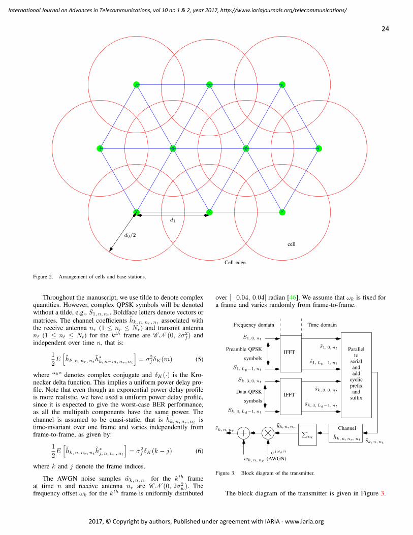
d1

Cell edge

cell

d0/2

Figure 2. Arrangement of cells and base stations.

Throughout the manuscript, we use tilde to denote complexquantities. However, complex QPSK symbols will be denotedwithout a tilde, e.g., S1, n, nt

. Boldface letters denote vectors or

matrices. The channel coefficients hk, n, nr, ntassociated with

the receive antenna nr (1 ≤ nr ≤ Nr) and transmit antennant (1 ≤ nt ≤ Nt) for the kth frame are C N (0, 2σ2

f ) andindependent over time n, that is:

1

2E[

hk, n, nr, nth∗

k, n−m,nr, nt

]

= σ2fδK(m) (5)

where “*” denotes complex conjugate and δK(·) is the Kro-necker delta function. This implies a uniform power delay pro-file. Note that even though an exponential power delay profileis more realistic, we have used a uniform power delay profile,since it is expected to give the worst-case BER performance,as all the multipath components have the same power. The

channel is assumed to be quasi-static, that is hk, n, nr, ntis

time-invariant over one frame and varies independently fromframe-to-frame, as given by:

1

2E[

hk, n, nr, nth∗

j, n, nr, nt

]

= σ2fδK(k − j) (6)

where k and j denote the frame indices.

The AWGN noise samples wk, n, nrfor the kth frame

at time n and receive antenna nr are C N (0, 2σ2w). The

frequency offset ωk for the kth frame is uniformly distributed

over [−0.04, 0.04] radian [46]. We assume that ωk is fixed fora frame and varies randomly from frame-to-frame.

IFFT

IFFT

Channel

hk, n, nr , nt

sk, 3, Ld−1, nt

Sk, 3, Ld−1, nt

Data QPSK

symbols

Sk, 3, 0, nt

Preamble QPSK

symbols

S1, Lp−1, nt

S1, 0, nt

s1, 0, nt

s1, Lp−1, nt

sk, 3, 0, nt

rk, n, nr

wk, n, nr(AWGN)

∑nt

yk, n, nr

e jωkn

sk, n, nt

Time domainFrequency domain

Parallelto

serialandadd

cyclicprefixand

suffix

Figure 3. Block diagram of the transmitter.

The block diagram of the transmitter is given in Figure 3.

24



With reference to Figs. 1(a) and 3, note that:

s1, n, nt=

1

Lp

Lp−1∑

i=0

S1, i, nte j 2πni/Lp

for 0 ≤ n ≤ Lp − 1

sk, 3, n, nt=

1

Ld

Ld−1∑

i=0

Sk, 3, i, nte j 2πni/Ld

for 0 ≤ n ≤ Ld − 1

sk, 2, n, nt= sk, 3, Ld−Lcp+n, nt

for 0 ≤ n ≤ Lcp − 1

s4, n, nt= s1, n, nt

for 0 ≤ n ≤ Lcs − 1

s5, n, nt= s1, n, nt

+ s4, n−Lp, nt. (7)

From (7), it is clear that the preamble is independent of theframe k. However, each transmit antenna has its own preamble,for the purpose of synchronization and channel estimation atthe receiver.

The preamble in the frequency domain, for each transmitantenna is generated as follows. Let πp(i), for 0 ≤ i ≤ Lp−1,denote the interleaver map for the preamble. Let

Sr =[

Sr, 0 . . . Sr, Lp−1

]T

Lp×1(8)

denote a random vector of QPSK symbols. The preamblevector for the transmit antenna nt is first initialized by

S1, nt=

[

S1, 0, nt. . . S1, Lp−1, nt

]T

Lp×1

= 0Lp×1. (9)

Next, we substitute

S1, πp(i4:i5), nt= Sr(i4 : i5). (10)

where i4 : i5 denotes the range of indices from i4 to i5, bothinclusive, and

i4 = (nt − 1)Lp/Nt

i5 = i4 + Lp/Nt − 1. (11)

Note that the preamble in the frequency domain for eachtransmit antenna has only Lp/Nt non-zero elements, the restof the elements are zero. Moreover, due to πp(·), the Lp/Nt

non-zero elements are randomly interspersed over the Lp

subcarriers in the frequency domain, for each transmit antenna.

By virtue of the preamble construction in (9), (10) and(11), the preambles in the frequency and time domains corre-sponding to transmit antennas nt and mt satisfy the relation(using Parseval’s energy theorem):

S1, i, ntS∗

1, i,mt= (2NtLp/Ld)δK(nt −mt)

for 0 ≤ i ≤ Lp − 1

⇒ s1, n, nt⊙Lp

s∗1,−n,mt=

0 for nt 6= mt,0 ≤ n ≤ Lp − 1

(2Lp/Ld)δK(n)for nt = mt

(12)

where “⊙Lp” denotes the Lp-point circular convolution. In

other words, the preambles corresponding to distinct transmitantennas are orthogonal over Lp samples. Moreover, the au-tocorrelation of the preambles in frequency and time domain,

can be approximated by a weighted Kronecker delta function(this condition is usually satisfied by random sequences havingzero-mean; the approximation gets better as Lp increases).

We assume Sk, 3, i, nt∈ {±1± j}. Since we require:

E[

|s1, n, nt|2]

= E[

|sk, 3, n, nt|2]

= 2/Ld∆= σ2

s (13)

we must have S1, i, nt∈√

LpNt/Ld (±1± j). In other words,the average power of the preamble part must be equal to theaverage power of the data part, in the time domain.

Due to the presence of the cyclic suffix in Figure 1 and(7), and due to (12), we have

s5, n, nt⋆ s∗1, Lp−1−n,mt

=

0 for Lp − 1 ≤ n ≤ Lp + Lhr − 2,nt 6= mt

(2Lp/Ld)δK(n− Lp + 1)for nt = mt

(14)

where “⋆” denotes linear convolution.

The signal for the kth frame and receive antenna nr canbe written as (for 0 ≤ n ≤ L+ Lh − 2):

rk, n, nr=

Nt∑

nt=1

(

sk, n, nt⋆ hk, n, nr, nt

)

e jωkn + wk, n, nr

= yk, n, nre jωkn + wk, n, nr

(15)

where sk, n, ntis depicted in Figure 1(a) and

yk, n, nr=

Nt∑

nt=1

sk, n, nt⋆ hk, n, nr, nt

. (16)

Note that any random carrier phase can be absorbed in thechannel impulse response.

The uplink and downlink transmissions between the mo-biles and base station could be carried out using time divisionduplex (TDD) or frequency division duplex (FDD). Timedivision (TDMA), frequency division (FDMA), code division(CDMA), orthogonal frequency division (OFDMA), for down-link transmissions and filterbank multicarrier (FBMC), foruplink transmissions [26], are the possible choices for multipleaccess (MA) techniques.

III. RECEIVER

In this section, we discuss the discrete-time receiver algo-rithms.

A. Start of Frame (SoF) and Coarse Frequency Offset Estimate

The start of frame (SoF) detection and coarse frequencyoffset estimation is performed for each receive antenna 1 ≤nr ≤ Nr and transmit antenna 1 ≤ nt ≤ Nt, as given by thefollowing rule (similar to (22) in [40] and (24) in [3]): choosethat value of m and νk which maximizes

∣

∣

∣

(

rk,m, nre−j νkm

)

⋆ s∗1, Lp−1−m,nt

∣

∣

∣. (17)

Let mk(·) denote the time instant and νk(·) denote the coarseestimate of the frequency offset (both of which are functionsof nr and nt), at which the maximum in (17) is obtained. Note

25



that (17) is a two-dimensional search over m and νk, whichcan be efficiently implemented in hardware, and there is a largescope for parallel processing. In particular, the search over νkinvolves dividing the range of ωk ([−0.04, 0.04]] radians) intoB1 frequency bins, and deciding in favour of that bin whichmaximizes (17). In our simulations, B1 = 64 [3] [40].

Note that in the absence of noise and due to the propertiesgiven in (14)

mk(nr, nt) = Lp − 1 + argmaxm

∣

∣

∣hk,m, nr, nt

∣

∣

∣(18)

where argmaxm corresponds to the value of m for which∣

∣

∣hk,m, nr, nt

∣

∣

∣is maximum. We also have

Lp − 1 ≤ mk(nr, nt) ≤ Lp + Lh − 2. (19)

If mk(·) lies outside the range in (19), the frame is declaredas erased (not detected). This implies that the peak in (17) isdue to noise, and not due to the channel. The results for SoFdetection at 0 dB SNR per bit for Lp = 512, 1024, 4096 aregiven in Figs. 4, 5, and 6, respectively, for Nt = Nr = 2.The parameter Z in the three figures denotes the correlationmagnitude given by (17).

The average value of the coarse frequency offset estimateis given by

ωk =

∑Nr

nr=1

∑Nt

nt=1 νk(nr, nt)

NrNt. (20)

B. Channel Estimation

We assume that the SoF has been estimated using (17)with outcome m0, k given by (assuming the condition in (19)is satisfied for all nr and nt):

m0, k = mk(1, 1)− Lp + 1 0 ≤ m0, k ≤ Lh − 1 (21)

and the frequency offset has been perfectly canceled [3] [40].Observe that any value of nr and nt can be used in thecomputation of (21). We have taken nr = nt = 1. Define

m1, k = m0, k + Lh − 1. (22)

For the sake of notational simplicity, we drop the subscript kin m1, k, and refer to it as m1. The steady-state, preamble part

of the received signal for the kth frame and receive antennanr can be written as:

rk,m1, nr=

Nt∑

nt=1

s5, nthk, nr, nt

+ wk,m1, nr(23)

where

rk,m1, nr=

[

rk,m1, nr. . . rk,m1+Lp−1, nr

]T

[Lp × 1] vector

wk,m1, nr=

[

wk,m1, nr. . . wk,m1+Lp−1, nr

]T

[Lp × 1] vector

hk, nr, nt=

[

hk, 0, nr, nt. . . hk, Lhr−1, nr, nt

]T

[Lhr × 1] vector

s5, nt=

s5, Lhr−1, nt. . . s5, 0, nt

... . . ....

s5, Lp+Lhr−2, nt. . . s5, Lp−1, nt

[Lp × Lhr] matrix (24)

where Lhr is the channel length assumed by the receiver (see(2)), s5, nt

is the channel estimation matrix and rk,m1, nris

the received signal vector after cancellation of the frequencyoffset. Observe that s5, nt

is independent of m1 and due to therelations in (12) and (14), we have

sH5,mt

s5, nt=

{

0Lhr×Lhrfor nt 6= mt

(2Lp/Ld)ILhrfor nt = mt

(25)

where ILhris an Lhr × Lhr identity matrix and 0Lhr×Lhr

is an Lhr × Lhr null matrix. The statement of the MLchannel estimation is as follows. Find hk, nr,mt

(the estimate

of hk, nr,mt) such that:

(

rk,m1, nr−

Nt∑

mt=1

s5,mthk, nr,mt

)H

(

rk,m1, nr−

Nt∑

mt=1

s5,mthk, nr,mt

)

(26)

is minimized. Differentiating with respect to h∗

k, nr,mtand

setting the result to zero yields [17] [47]:

hk, nr,mt=(

sH5,mt

s5,mt

)−1sH5,mt

rk,m1, nr. (27)

Observe that when m0, k = Lh−1 in (21), and noise is absent(see (29) in [40] and (35) in [3]), we obtain:

hk, nr,mt

=[

hk, 0, nr,mt. . . hk, Lh−1, nr,mt

0 . . . 0]T

. (28)

Similarly, when m0, k = 0 and in the absence of noise:

hk, nr,mt

=[

0 . . . 0 hk, 0, nr,mt. . . hk, Lh−1, nr,mt

]T. (29)

To see the effect of noise on the channel estimate in (27),consider

u =(

sH5,mt

s5,mt

)−1sH5,mt

wk,m1, nr. (30)

It can be shown that

E[

uuH]

=σ2wLd

LpILhr

∆= 2σ2

uILhr. (31)

Therefore, the variance of the ML channel estimate (σ2u) tends

to zero as Lp → ∞ and Ld is kept fixed. Conversely, whenLd is increased keeping Lp fixed, there is noise enhancement[2] [3]. The magnitude spectrum of the actual and estimatedchannel for various preamble lengths are shown in Figs. 7, 8and 9 for Nt = Nr = 2 and 0 dB average SNR per bit. Note

that Hk, i, nr, ntdenotes the Ld-point discrete Fourier transform

(DFT) of hk, n, nr, ntin (5).

C. Fine Frequency Offset Estimation

The fine frequency offset estimate is obtained using thefollowing rule: choose that value of time instant m andfrequency offset νk, f which maximizes:∣

∣

∣

(

rk,m, nre−j (ωk+νk, f )m

)

⋆ y∗1, k, L2−1−m,nr, nt

∣

∣

∣(32)

26



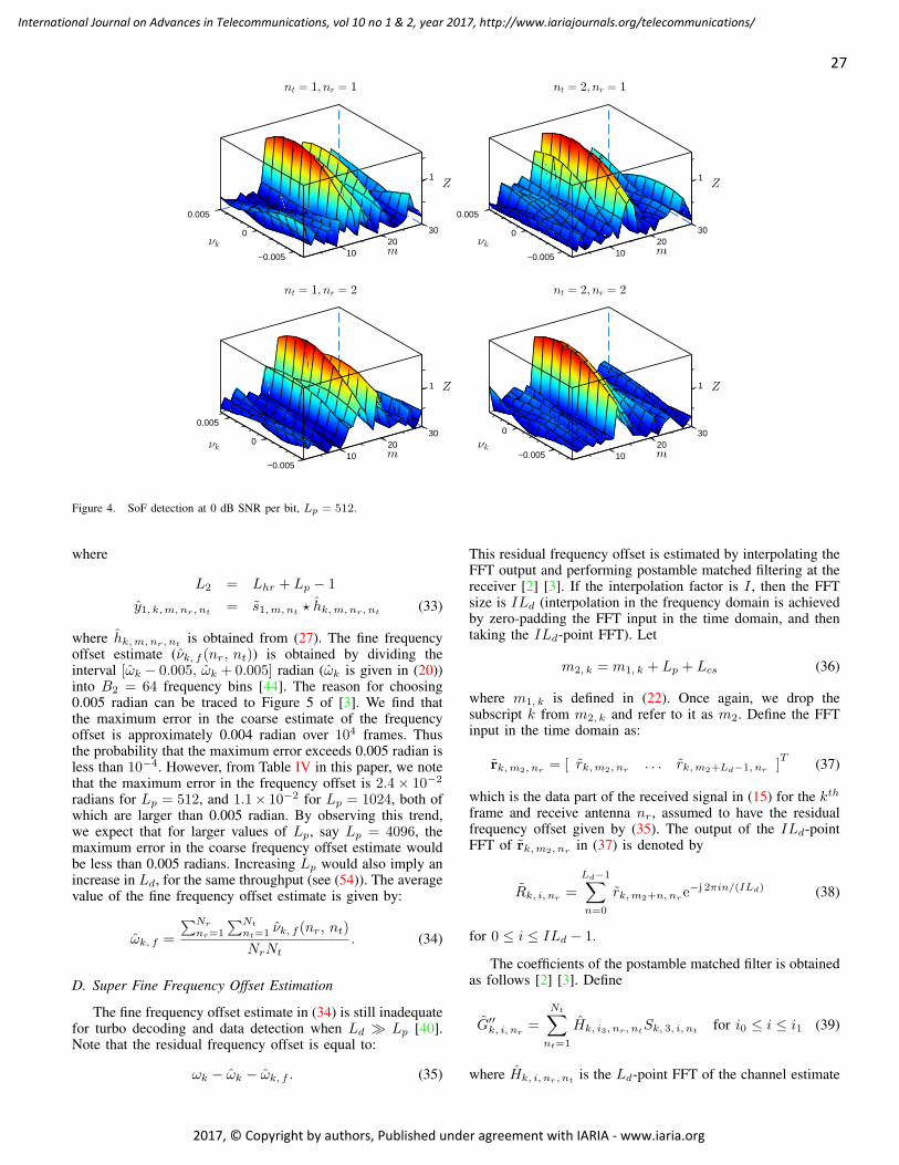
2010

300

−0.005

0.005

1

2010

300

−0.005

0.005

1

2010

300

−0.005

0.005

1

2010

300

−0.005

1

Figure 4. SoF detection at 0 dB SNR per bit, Lp = 512.

where

L2 = Lhr + Lp − 1

y1, k,m, nr, nt= s1,m, nt

⋆ hk,m, nr, nt(33)

where hk,m, nr, ntis obtained from (27). The fine frequency

offset estimate (νk, f (nr, nt)) is obtained by dividing theinterval [ωk − 0.005, ωk + 0.005] radian (ωk is given in (20))into B2 = 64 frequency bins [44]. The reason for choosing0.005 radian can be traced to Figure 5 of [3]. We find thatthe maximum error in the coarse estimate of the frequencyoffset is approximately 0.004 radian over 104 frames. Thusthe probability that the maximum error exceeds 0.005 radian isless than 10−4. However, from Table IV in this paper, we notethat the maximum error in the frequency offset is 2.4× 10−2

radians for Lp = 512, and 1.1× 10−2 for Lp = 1024, both ofwhich are larger than 0.005 radian. By observing this trend,we expect that for larger values of Lp, say Lp = 4096, themaximum error in the coarse frequency offset estimate wouldbe less than 0.005 radians. Increasing Lp would also imply anincrease in Ld, for the same throughput (see (54)). The averagevalue of the fine frequency offset estimate is given by:

ωk, f =

∑Nr

nr=1

∑Nt

nt=1 νk, f (nr, nt)

NrNt. (34)

D. Super Fine Frequency Offset Estimation

The fine frequency offset estimate in (34) is still inadequatefor turbo decoding and data detection when Ld ≫ Lp [40].Note that the residual frequency offset is equal to:

ωk − ωk − ωk, f . (35)

This residual frequency offset is estimated by interpolating theFFT output and performing postamble matched filtering at thereceiver [2] [3]. If the interpolation factor is I , then the FFTsize is ILd (interpolation in the frequency domain is achievedby zero-padding the FFT input in the time domain, and thentaking the ILd-point FFT). Let

m2, k = m1, k + Lp + Lcs (36)

where m1, k is defined in (22). Once again, we drop thesubscript k from m2, k and refer to it as m2. Define the FFTinput in the time domain as:

rk,m2, nr= [ rk,m2, nr

. . . rk,m2+Ld−1, nr ]T

(37)

which is the data part of the received signal in (15) for the kth

frame and receive antenna nr, assumed to have the residualfrequency offset given by (35). The output of the ILd-pointFFT of rk,m2, nr

in (37) is denoted by

Rk, i, nr=

Ld−1∑

n=0

rk,m2+n, nre−j 2πin/(ILd) (38)

for 0 ≤ i ≤ ILd − 1.

The coefficients of the postamble matched filter is obtainedas follows [2] [3]. Define

G′′

k, i, nr=

Nt∑

nt=1

Hk, i3, nr, ntSk, 3, i, nt

for i0 ≤ i ≤ i1 (39)

where Hk, i, nr, ntis the Ld-point FFT of the channel estimate

27



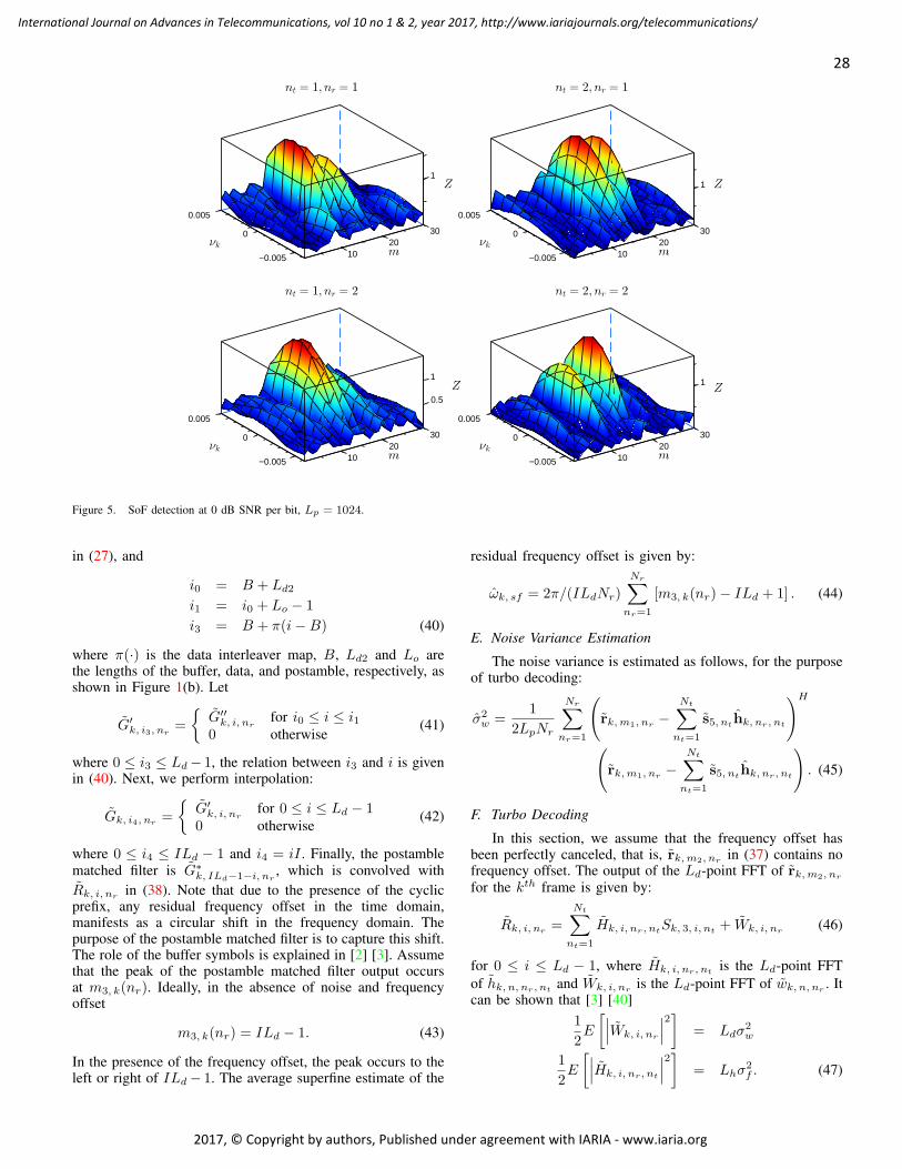
2010

300

−0.005

0.005

1

2010

300

−0.005

0.005

1

2010

300

−0.005

0.005

1

0.5

2010

300

−0.005

0.005

1


in (27), and

i0 = B + Ld2

i1 = i0 + Lo − 1

i3 = B + π(i−B) (40)

where π(·) is the data interleaver map, B, Ld2 and Lo arethe lengths of the buffer, data, and postamble, respectively, asshown in Figure 1(b). Let

G′

k, i3, nr=

{

G′′

k, i, nrfor i0 ≤ i ≤ i1

0 otherwise(41)

where 0 ≤ i3 ≤ Ld − 1, the relation between i3 and i is givenin (40). Next, we perform interpolation:

Gk, i4, nr=

{

G′

k, i, nrfor 0 ≤ i ≤ Ld − 1

0 otherwise(42)

where 0 ≤ i4 ≤ ILd − 1 and i4 = iI . Finally, the postamble

matched filter is G∗

k, ILd−1−i, nr, which is convolved with

Rk, i, nrin (38). Note that due to the presence of the cyclic

prefix, any residual frequency offset in the time domain,manifests as a circular shift in the frequency domain. Thepurpose of the postamble matched filter is to capture this shift.The role of the buffer symbols is explained in [2] [3]. Assumethat the peak of the postamble matched filter output occursat m3, k(nr). Ideally, in the absence of noise and frequencyoffset

m3, k(nr) = ILd − 1. (43)

In the presence of the frequency offset, the peak occurs to theleft or right of ILd − 1. The average superfine estimate of the

residual frequency offset is given by:

ωk, sf = 2π/(ILdNr)

Nr∑

nr=1

[m3, k(nr)− ILd + 1] . (44)

E. Noise Variance Estimation

The noise variance is estimated as follows, for the purposeof turbo decoding:

σ2w =

1

2LpNr

Nr∑

nr=1

(

rk,m1, nr−

Nt∑

nt=1

s5, nthk, nr, nt

)H

(

rk,m1, nr−

Nt∑

nt=1

s5, nthk, nr, nt

)

. (45)

F. Turbo Decoding

In this section, we assume that the frequency offset hasbeen perfectly canceled, that is, rk,m2, nr

in (37) contains nofrequency offset. The output of the Ld-point FFT of rk,m2, nr

for the kth frame is given by:

Rk, i, nr=

Nt∑

nt=1

Hk, i, nr, ntSk, 3, i, nt

+ Wk, i, nr(46)

for 0 ≤ i ≤ Ld − 1, where Hk, i, nr, ntis the Ld-point FFT

of hk, n, nr, ntand Wk, i, nr

is the Ld-point FFT of wk, n, nr. It

can be shown that [3] [40]

1

2E

[

∣

∣

∣Wk, i, nr

∣

∣

∣

2]

= Ldσ2w

1

2E

[

∣

∣

∣Hk, i, nr, nt

∣

∣

∣

2]

= Lhσ2f . (47)

28



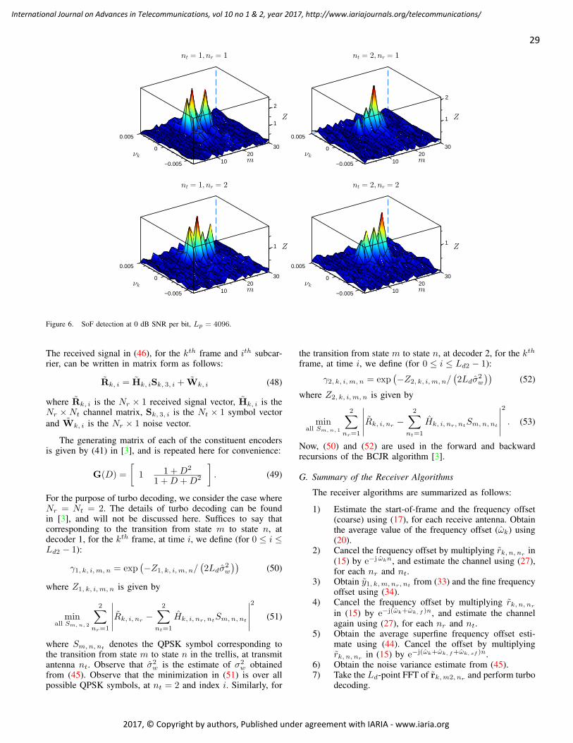
2010

300

−0.005

0.005

2

1

2010

300

−0.005

0.005

2

1

2010

300

−0.005

0.005

1

2010

300

−0.005

0.005

1


The received signal in (46), for the kth frame and ith subcar-rier, can be written in matrix form as follows:

Rk, i = Hk, iSk, 3, i + Wk, i (48)

where Rk, i is the Nr × 1 received signal vector, Hk, i is theNr ×Nt channel matrix, Sk, 3, i is the Nt × 1 symbol vector

and Wk, i is the Nr × 1 noise vector.

The generating matrix of each of the constituent encodersis given by (41) in [3], and is repeated here for convenience:

G(D) =

[

1 1 +D2

1 +D +D2

]

. (49)

For the purpose of turbo decoding, we consider the case whereNr = Nt = 2. The details of turbo decoding can be foundin [3], and will not be discussed here. Suffices to say thatcorresponding to the transition from state m to state n, atdecoder 1, for the kth frame, at time i, we define (for 0 ≤ i ≤Ld2 − 1):

γ1, k, i,m, n = exp(

−Z1, k, i,m, n/(

2Ldσ2w

))

(50)

where Z1, k, i,m, n is given by

minall Sm,n, 2

2∑

nr=1

∣

∣

∣

∣

∣

Rk, i, nr−

2∑

nt=1

Hk, i, nr, ntSm,n, nt

∣

∣

∣

∣

∣

2

(51)

where Sm,n, ntdenotes the QPSK symbol corresponding to

the transition from state m to state n in the trellis, at transmitantenna nt. Observe that σ2

w is the estimate of σ2w obtained

from (45). Observe that the minimization in (51) is over allpossible QPSK symbols, at nt = 2 and index i. Similarly, for

the transition from state m to state n, at decoder 2, for the kth

frame, at time i, we define (for 0 ≤ i ≤ Ld2 − 1):

γ2, k, i,m, n = exp(

−Z2, k, i,m, n/(

2Ldσ2w

))

(52)

where Z2, k, i,m, n is given by

minall Sm,n, 1

2∑

nr=1

∣

∣

∣

∣

∣

Rk, i, nr−

2∑

nt=1

Hk, i, nr, ntSm,n, nt

∣

∣

∣

∣

∣

2

. (53)

Now, (50) and (52) are used in the forward and backwardrecursions of the BCJR algorithm [3].

G. Summary of the Receiver Algorithms

The receiver algorithms are summarized as follows:

1) Estimate the start-of-frame and the frequency offset(coarse) using (17), for each receive antenna. Obtainthe average value of the frequency offset (ωk) using(20).

2) Cancel the frequency offset by multiplying rk, n, nrin

(15) by e−j ωkn, and estimate the channel using (27),for each nr and nt.

3) Obtain y1, k,m, nr, ntfrom (33) and the fine frequency

offset using (34).4) Cancel the frequency offset by multiplying rk, n, nr

in (15) by e−j(ωk+ωk, f )n, and estimate the channelagain using (27), for each nr and nt.

5) Obtain the average superfine frequency offset esti-mate using (44). Cancel the offset by multiplyingrk, n, nr

in (15) by e−j(ωk+ωk, f+ωk, sf )n.6) Obtain the noise variance estimate from (45).7) Take the Ld-point FFT of rk,m2, nr

and perform turbodecoding.

29



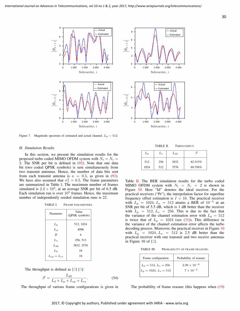
0 2 000 4 0001 000 3 000

0

2

4

6

8Actual

Estimated

0 2 000 4 0001 000 3 000

0

2

4

6

8 Actual

Estimated

0 2 000 4 0001 000 3 000

0

2

4

6

8Actual

Estimated

0 2 000 4 0001 000 3 000

0

2

4

6Actual

Estimated

Figure 7. Magnitude spectrum of estimated and actual channel, Lp = 512.

H. Simulation Results

In this section, we present the simulation results for theproposed turbo coded MIMO OFDM system with Nt = Nr =2. The SNR per bit is defined in (92). Note that one databit (two coded QPSK symbols) is sent simultaneously fromtwo transmit antennas. Hence, the number of data bits sentfrom each transmit antenna is κ = 0.5, as given in (92).We have also assumed that σ2

f = 0.5. The frame parametersare summarized in Table I. The maximum number of framessimulated is 2.2 × 104, at an average SNR per bit of 6.5 dB.Each simulation run is over 103 frames. Hence, the maximumnumber of independently seeded simulation runs is 22.

TABLE I. FRAME PARAMETERS.

Lp

Ld

B

Lo

Ld2

Lh

Lcp = Lcs

512, 1024

4096

4

256, 512

10

Value(QPSK symbols)

Parameter

18

3832, 3576

The throughput is defined as [2] [3]:

T =Ld2

Ld + Lp + Lcp + Lcs. (54)

The throughput of various frame configurations is given in

TABLE II. THROUGHPUT.

Lp Lo Ld2 T

512 256 3832 82.515%

1024 512 3576 69.356%

Table II. The BER simulation results for the turbo codedMIMO OFDM system with Nt = Nr = 2 is shown inFigure 10. Here “Id” denotes the ideal receiver. For thepractical receivers (“Pr”), the interpolation factor for superfinefrequency offset estimation is I = 16. The practical receiverwith Lp = 1024, Lo = 512 attains a BER of 10−5 at anSNR per bit of 5.5 dB, which is 1 dB better than the receiverwith Lp = 512, Lo = 256. This is due to the fact thatthe variance of the channel estimation error with Lp = 512is twice that of Lp = 1024 (see (31)). This difference inthe variance of the channel estimation error affects the turbodecoding process. Moreover, the practical receiver in Figure 10with Lp = 1024, Lo = 512 is 2.5 dB better than thepractical receiver with one transmit and two receive antennasin Figure 10 of [2].

TABLE III. PROBABILITY OF FRAME ERASURE.

Lp = 512, Lo = 256

Lp = 1024, Lo = 512

Probability of erasure

2.98× 10−2

7× 10−4

Frame configuration

The probability of frame erasure (this happens when (19)

30



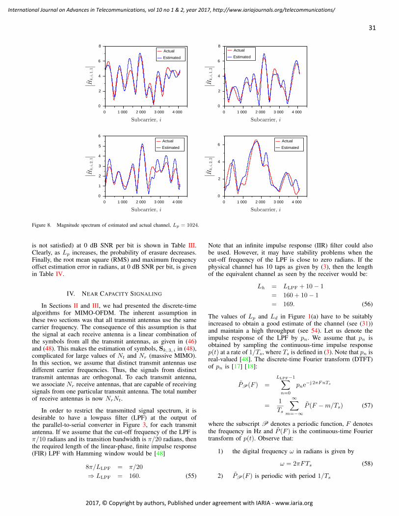
0 2 000 4 0001 000 3 000

0

2

4

6

8Actual

Estimated

0 2 000 4 0001 000 3 000

0

2

4

6

8Actual

Estimated

0 2 000 4 0001 000 3 000

0

2

4

6

1

3

5Actual

Estimated

0 2 000 4 0001 000 3 000

0

2

4

6Actual

Estimated


is not satisfied) at 0 dB SNR per bit is shown in Table III.Clearly, as Lp increases, the probability of erasure decreases.Finally, the root mean square (RMS) and maximum frequencyoffset estimation error in radians, at 0 dB SNR per bit, is givenin Table IV.

IV. NEAR CAPACITY SIGNALING

In Sections II and III, we had presented the discrete-timealgorithms for MIMO-OFDM. The inherent assumption inthese two sections was that all transmit antennas use the samecarrier frequency. The consequence of this assumption is thatthe signal at each receive antenna is a linear combination ofthe symbols from all the transmit antennas, as given in (46)and (48). This makes the estimation of symbols, Sk, 3, i in (48),complicated for large values of Nt and Nr (massive MIMO).In this section, we assume that distinct transmit antennas usedifferent carrier frequencies. Thus, the signals from distincttransmit antennas are orthogonal. To each transmit antenna,we associate Nr receive antennas, that are capable of receivingsignals from one particular transmit antenna. The total numberof receive antennas is now NrNt.

In order to restrict the transmitted signal spectrum, it isdesirable to have a lowpass filter (LPF) at the output ofthe parallel-to-serial converter in Figure 3, for each transmitantenna. If we assume that the cut-off frequency of the LPF isπ/10 radians and its transition bandwidth is π/20 radians, thenthe required length of the linear-phase, finite impulse response(FIR) LPF with Hamming window would be [48]

8π/LLPF = π/20

⇒ LLPF = 160. (55)

Note that an infinite impulse response (IIR) filter could alsobe used. However, it may have stability problems when thecut-off frequency of the LPF is close to zero radians. If thephysical channel has 10 taps as given by (3), then the lengthof the equivalent channel as seen by the receiver would be:

Lh = LLPF + 10− 1

= 160 + 10− 1

= 169. (56)

The values of Lp and Ld in Figure 1(a) have to be suitablyincreased to obtain a good estimate of the channel (see (31))and maintain a high throughput (see 54). Let us denote theimpulse response of the LPF by pn. We assume that pn isobtained by sampling the continuous-time impulse responsep(t) at a rate of 1/Ts, where Ts is defined in (3). Note that pn isreal-valued [48]. The discrete-time Fourier transform (DTFT)of pn is [17] [18]:

PP(F ) =

LLPF−1∑

n=0

pne−j 2πFnTs

=1

Ts

∞∑

m=−∞

P (F −m/Ts) (57)

where the subscript P denotes a periodic function, F denotes

the frequency in Hz and P (F ) is the continuous-time Fouriertransform of p(t). Observe that:

1) the digital frequency ω in radians is given by

ω = 2πFTs (58)

2) PP(F ) is periodic with period 1/Ts

31



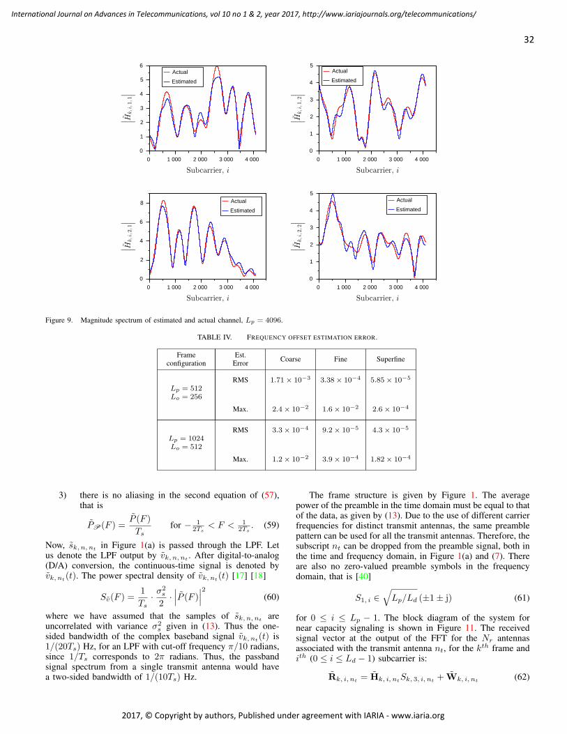
0 2 000 4 0001 000 3 000

0

2

4

6

1

3

5Actual

Estimated

0 2 000 4 0001 000 3 000

0

2

4

1

3

5Actual

Estimated

0 2 000 4 0001 000 3 000

0

2

4

6

8 Actual

Estimated

0 2 000 4 0001 000 3 000

0

2

4

1

3

5Actual

Estimated


TABLE IV. FREQUENCY OFFSET ESTIMATION ERROR.

5.85× 10−5

SuperfineCoarse

1.71× 10−3

Fine

3.38× 10−4

2.4× 10−2 1.6× 10−2 2.6× 10−4

RMS

Max.

Est.Errorconfiguration

Frame

Lp = 512Lo = 256

Lp = 1024Lo = 512

3.3× 10−4 9.2× 10−5 4.3× 10−5RMS

Max. 1.2× 10−2 3.9× 10−4 1.82× 10−4

3) there is no aliasing in the second equation of (57),that is

PP(F ) =P (F )

Tsfor − 1

2Ts< F < 1

2Ts. (59)

Now, sk, n, ntin Figure 1(a) is passed through the LPF. Let

us denote the LPF output by vk, n, nt. After digital-to-analog

(D/A) conversion, the continuous-time signal is denoted byvk, nt

(t). The power spectral density of vk, nt(t) [17] [18]

Sv(F ) =1

Ts· σ

2s

2·∣

∣

∣P (F )

∣

∣

∣

2

(60)

where we have assumed that the samples of sk, n, ntare

uncorrelated with variance σ2s given in (13). Thus the one-

sided bandwidth of the complex baseband signal vk, nt(t) is

1/(20Ts) Hz, for an LPF with cut-off frequency π/10 radians,since 1/Ts corresponds to 2π radians. Thus, the passbandsignal spectrum from a single transmit antenna would havea two-sided bandwidth of 1/(10Ts) Hz.

The frame structure is given by Figure 1. The averagepower of the preamble in the time domain must be equal to thatof the data, as given by (13). Due to the use of different carrierfrequencies for distinct transmit antennas, the same preamblepattern can be used for all the transmit antennas. Therefore, thesubscript nt can be dropped from the preamble signal, both inthe time and frequency domain, in Figure 1(a) and (7). Thereare also no zero-valued preamble symbols in the frequencydomain, that is [40]

S1, i ∈√

Lp/Ld (±1± j) (61)

for 0 ≤ i ≤ Lp − 1. The block diagram of the system fornear capacity signaling is shown in Figure 11. The receivedsignal vector at the output of the FFT for the Nr antennasassociated with the transmit antenna nt, for the kth frame andith (0 ≤ i ≤ Ld − 1) subcarrier is:

Rk, i, nt= Hk, i, nt

Sk, 3, i, nt+ Wk, i, nt

(62)

32



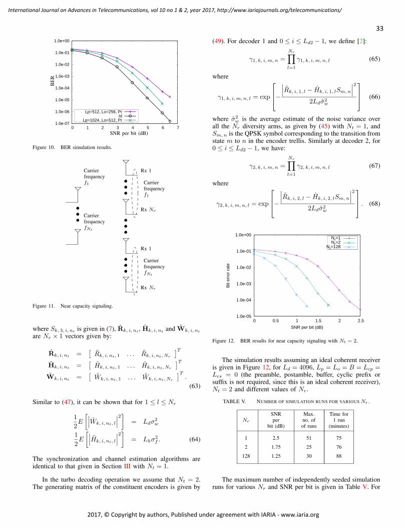
1.0e-07

1.0e-06

1.0e-05

1.0e-04

1.0e-03

1.0e-02

1.0e-01

1.0e+00

0 1 2 3 4 5 6 7

Lp=512, Lo=256, PrId

Lp=1024, Lo=512, Pr

SNR per bit (dB)

BE

R

Figure 10. BER simulation results.

f1

fNt

f1

fNt

Carrierfrequency

Carrierfrequency

Carrierfrequency

Carrierfrequency

Rx 1

Rx Nr

Rx 1

Rx Nr

Figure 11. Near capacity signaling.

where Sk, 3, i, ntis given in (7), Rk, i, nt

, Hk, i, ntand Wk, i, nt

are Nr × 1 vectors given by:

Rk, i, nt=

[

Rk, i, nt, 1 . . . Rk, i, nt, Nr

]T

Hk, i, nt=

[

Hk, i, nt, 1 . . . Hk, i, nt, Nr

]T

Wk, i, nt=

[

Wk, i, nt, 1 . . . Wk, i, nt, Nr

]T.

(63)

Similar to (47), it can be shown that for 1 ≤ l ≤ Nr

1

2E

[

∣

∣

∣Wk, i, nt, l

∣

∣

∣

2]

= Ldσ2w

1

2E

[

∣

∣

∣Hk, i, nt, l

∣

∣

∣

2]

= Lhσ2f . (64)

The synchronization and channel estimation algorithms areidentical to that given in Section III with Nt = 1.

In the turbo decoding operation we assume that Nt = 2.The generating matrix of the constituent encoders is given by

(49). For decoder 1 and 0 ≤ i ≤ Ld2 − 1, we define [2]:

γ1, k, i,m, n =

Nr∏

l=1

γ1, k, i,m, n, l (65)

where

γ1, k, i,m, n, l = exp

−

∣

∣

∣Rk, i, 1, l − Hk, i, 1, lSm,n

∣

∣

∣

2

2Ldσ2w

(66)

where σ2w is the average estimate of the noise variance over

all the Nr diversity arms, as given by (45) with Nt = 1, andSm,n is the QPSK symbol corresponding to the transition fromstate m to n in the encoder trellis. Similarly at decoder 2, for0 ≤ i ≤ Ld2 − 1, we have:

γ2, k, i,m, n =

Nr∏

l=1

γ2, k, i,m, n, l (67)

where

γ2, k, i,m, n, l = exp

−

∣

∣

∣Rk, i, 2, l − Hk, i, 2, lSm,n

∣

∣

∣

2

2Ldσ2w

. (68)

1.0e-05

1.0e-04

1.0e-03

1.0e-02

1.0e-01

1.0e+00

0 0.5 1 1.5 2 2.5

Bit

erro

r ra

te

SNR per bit (dB)

Nr=1Nr=2

Nr=128

Figure 12. BER results for near capacity signaling with Nt = 2.

The simulation results assuming an ideal coherent receiveris given in Figure 12, for Ld = 4096, Lp = Lo = B = Lcp =Lcs = 0 (the preamble, postamble, buffer, cyclic prefix orsuffix is not required, since this is an ideal coherent receiver),Nt = 2 and different values of Nr.

TABLE V. NUMBER OF SIMULATION RUNS FOR VARIOUS Nr .

Nr

1

2

128

Time for1 run

75

76

88

(minutes)

SNRper

bit (dB)

2.5

1.75

1.25

Max.no. ofof runs

51

25

30

The maximum number of independently seeded simulationruns for various Nr and SNR per bit is given in Table V. For

33



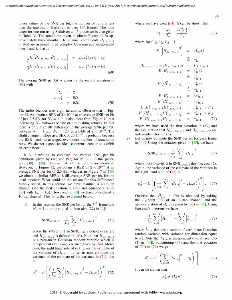
lower values of the SNR per bit, the number of runs is lessthan the maximum. Each run is over 103 frames. The timetaken for one run using Scilab on an i5 processor is also givenin Table V. The total time taken to obtain Figure 12 is ap-

proximately three months. The channel coefficients Hk, i, nt, l

in (63) are assumed to be complex Gaussian and independentover i and l, that is

1

2E[

Hk, i1, nt, lH∗

k, i2, nt, l

]

= Lhσ2fδK(i1 − i2)

1

2E[

Hk, i, nt, l1H∗

k, i, nt, l2

]

= Lhσ2fδK(l1 − l2).

(69)

The average SNR per bit is given by the second equation in(92) with

Pav = 2

Lhσ2f = 0.5

κ = 0.5. (70)

The turbo decoder uses eight iterations. Observe that in Fig-ure 12, we obtain a BER of 2×10−5 at an average SNR per bitof just 2.5 dB, for Nr = 1. It is also clear from Figure 12 thatincreasing Nr follows the law of diminishing returns. In factthere is only 1.25 dB difference in the average SNR per bit,between Nr = 1 and Nr = 128, at a BER of 2 × 10−5. Theslight change in slope at a BER of 2×10−5 is probably becausethe BER needs to averaged over more number of simulationruns. We do not expect an ideal coherent detector to exhibitan error floor.

It is interesting to compare the average SNR per bitdefinitions given by (70) and (92) for Nr = 1 in this paper,with (38) in [40]. Observe that both definitions are identical.However, in Figure 12, we obtain a BER of 2 × 10−5 at anaverage SNR per bit of 2.5 dB, whereas in Figure 7 of [40]we obtain a similar BER at 8 dB average SNR per bit, for theideal receiver. What could be the reason for this difference?Simply stated, in this section we have assumed a 4096-tapchannel (see the first equation in (69) and equation (37) in[40] with Lh = Ld). However, in [40] we have considered a10-tap channel. This is further explained below.

1) In this section, the SNR per bit for the kth frame andNr = 1 is proportional to (see also (22) in [2])

SNRk, bit, 1 ∝ 1

Ld

Ld−1∑

i=0

∣

∣

∣Hk, i, nt, 1

∣

∣

∣

2

(71)

where the subscript 1 in SNRk, bit, 1 denotes case (1)

and Hk, i, nt, 1 is defined in (63). Note that Hk, i, nt, 1

is a zero-mean Gaussian random variable which isindependent over i and variance given by (64). More-over, the right hand side of (71) gives the estimate of

the variance of Hk, i, nt, 1. Let us now compute thevariance of the estimate of the variance in (71), thatis

σ21 = E

(

1

Ld

Ld−1∑

i=0

∣

∣

∣Hk, i, nt, 1

∣

∣

∣

2

− 2Lhσ2f

)2

(72)

where we have used (64). It can be shown that

σ21 =

σ4H

Ld=

4L2hσ

4f

Ld(73)

where for 0 ≤ i ≤ Ld − 1

E

[

∣

∣

∣Hk, i, nt, 1

∣

∣

∣

2]

= 2Lhσ2f

∆= σ2

H

Hk, i, nt, 1, I + jHk, i, nt, 1, Q = Hk, i, nt, 1

E[

H2k, i, nt, 1, I

]

= σ2H/2

∆= σ2

H, 1

E[

H2k, i, nt, 1, Q

]

= σ2H/2

∆= σ2

H, 1

E[

H4k, i, nt, 1, I

]

= 3σ4H, 1

E[

H4k, i, nt, 1, Q

]

= 3σ4H, 1

E[

H2k, i, nt, 1, IH

2k, j, nt, 1, I

]

= σ4H, 1 i 6= j

E[

H2k, i, nt, 1, QH

2k, j, nt, 1, Q

]

= σ4H, 1 i 6= j

E[

H2k, i, nt, 1, IH

2k, j, nt, 1, Q

]

= σ4H, 1 (74)

where we have used the first equation in (69) andthe assumption that Hk, i, nt, 1, I and Hk, j, nt, 1, Q areindependent for all i, j.

2) Let us now compute the SNR per bit for each framein [40]. Using the notation given in [40], we have

SNRk, bit, 2 ∝ 1

Ld

Ld−1∑

i=0

∣

∣

∣Hk, i

∣

∣

∣

2

(75)

where the subscript 2 in SNRk, bit, 2 denotes case (2).Again, the variance of the estimate of the variance inthe right hand side of (75) is

σ22 = E

(

1

Ld

Ld−1∑

i=0

∣

∣

∣Hk, i

∣

∣

∣

2

− 2Lhσ2f

)2

. (76)

Observe that Hk, i in (76) is obtained by takingthe Ld-point FFT of an Lh-tap channel, and the

autocorrelation of Hk, i is given by (37) in [40]. UsingParseval’s theorem we have

1

Ld

Ld−1∑

i=0

∣

∣

∣Hk, i

∣

∣

∣

2

=

Lh−1∑

n=0

∣

∣

∣hk, n

∣

∣

∣

2

(77)

where hk, n denotes a sample of zero-mean Gaussianrandom variable with variance per dimension equal

to σ2f . Note that hk, n is independent over n (see also

(1) in [40]). Substituting (77) and the first equationof (74) in (76) we get

σ22 = E

(

Lh−1∑

n=0

∣

∣

∣hk, n

∣

∣

∣

2

− σ2H

)2

. (78)

It can be shown that

σ22 = 4Lhσ

4f (79)

34



where we have used the following relations:

E

[

∣

∣

∣hk, n

∣

∣

∣

2]

= 2σ2f

hk, n, I + jhk, n,Q = hk, n

E[

h2k, n, I

]

= σ2f

E[

h2k, n,Q

]

= σ2f

E[

h4k, n, I

]

= 3σ4f

E[

h4k, n,Q

]

= 3σ4f

E[

h2k, n, Ih

2k,m, I

]

= σ4f n 6= m

E[

h2k, n,Qh

2k,m,Q

]

= σ4f n 6= m

E[

h2k, n, Ih

2k,m,Q

]

= σ4f (80)

where we have assumed that hk, n, I and hk,m,Q areindependent for all n, m.

Substituting

Lh = 10

Ld = 4096 (81)

in (74) and (80) we obtain

σ21 = 0.1σ4

f

σ22 = 40σ4

f . (82)

Thus we find that the variation in the SNR per bit for eachframe is 400 times larger in case (2) than in case (1). Therefore,in case (2) there are many frames whose SNR per bit is muchsmaller than the average value given by (92), resulting in alarge number of bit errors. Conversely, the average SNR perbit in case (2) needs to be much higher than in case (1) forthe same BER.

V. CONCLUSIONS

Discrete-time algorithms for the coherent detection of turbocoded MIMO OFDM system are presented. Simulations resultsfor a 2× 2 turbo coded MIMO OFDM system indicate that aBER of 10−5, is obtained at an SNR per bit of just 5.5 dB,which is a 2.5 dB improvement over the performance given inthe literature. The minimum average SNR per bit for error-freetransmission over fading channels is derived and shown to beequal to −1.6 dB, which is the same as that for the AWGNchannel.

Finally, an ideal near capacity signaling is proposed, whereeach transmit antenna uses a different carrier frequency. Sim-ulation results for the ideal coherent receiver show that it ispossible to achieve a BER of 2×10−5 at an average SNR perbit equal to 2.5 dB, with two transmit and two receive antennas.When the number of receive antennas for each transmit antennais increased to 128, the average SNR per bit required to attaina BER of 2× 10−5 is 1.25 dB. The spectral efficiency of theproposed near capacity system is 1 bit/sec/Hz. Higher spectralefficiency can be obtained by increasing the number of transmitantennas with no loss in BER performance. A pulse shapingtechnique is also proposed to reduce the bandwidth of thetransmitted signal.

Future work could address the issues of peak-to-averagepower ratio (PAPR).

APPENDIX

A. The Minimum Average SNR per bit for Error-free Trans-mission over Fading Channels

In this appendix, we derive the minimum average SNR perbit for error-free transmission over MIMO fading channels.Consider the signal

rn = xn + wn for 0 ≤ n < N (83)

where xn is the transmitted signal (message) and wn denotessamples of zero-mean noise, not necessarily Gaussian. Allthe terms in (83) are complex-valued or two-dimensionaland are transmitted over one complex dimension. Here theterm dimension refers to a communication link between thetransmitter and the receiver carrying only real-valued signals.We also assume that xn and wn are ergodic random processes,that is, the time average statistics is equal to the ensembleaverage. The time-averaged signal power over two-dimensionsis given by, for large values of N :

1

N

N−1∑

n=0

|xn|2 = P ′

av. (84)

The time-averaged noise power per dimension is

1

2N

N−1∑

n=0

|wn|2 = σ′2w =

1

2N

N−1∑

n=0

|rn − xn|2 . (85)

The received signal power over two-dimensions is

1

N

N−1∑

n=0

|rn|2 =1

N

N−1∑

n=0

|xn + wn|2

=1

N

N−1∑

n=0

|xn|2 + |wn|2

= P ′

av + 2σ′2w

= E[

|xn + wn|2]

(86)

where we have assumed independence between xn and wn

and the fact that wn has zero-mean. Note that in (86) it isnecessary that either xn or wn or both, have zero-mean.

Next, we observe that (85) is the expression for a 2N -

dimensional noise hypersphere with radius σ′

w

√2N . Similarly,

(86) is the expression for a 2N -dimensional received signal

hypersphere with radius

√

N(P ′

av + 2σ′2w).

Now, the problem statement is: how many noise hyper-spheres (messages) can fit into the received signal hypersphere,such that the noise hyperspheres do not overlap (reliable

decoding), for a given N , P ′

av and σ′2w? The solution lies in the

volume of the two hyperspheres. Note that a 2N -dimensionalhypersphere of radius R has a volume proportional to R2N .Therefore, the number of possible messages is

M =

(

N(

P ′

av + 2σ′2w

))N

(

2Nσ′2w

)N=

(

P ′

av + 2σ′2w

2σ′2w

)N

(87)

over N samples (transmissions). The number of bits requiredto represent each message is log2(M), over N transmissions.

35



Therefore, the number of bits per transmission, defined as thechannel capacity, is given by [49]

C =1

Nlog2(M)

= log2

(

1 +P ′

av

2σ′2w

)

bits per transmission (88)

over two dimensions or one complex dimension (here again theterm “dimension” implies a communication link between thetransmitter and receiver, carrying only real-valued signals. Thisis not to be confused with the 2N -dimensional hyperspherementioned earlier or the M -dimensional orthogonal constella-tions in [18]).

Proposition A.1: Clearly, the channel capacity is additiveover the number of dimensions. In other words, channelcapacity over D dimensions, is equal to the sum of thecapacities over each dimension, provided the information isindependent across dimensions [2]. Independence of informa-tion also implies that, the bits transmitted over one dimensionis not the interleaved version of the bits transmitted over anyother dimension.

Proposition A.2: Conversely, if C bits per transmission aresent over 2Nr dimensions, (Nr complex dimensions), it seemsreasonable to assume that each complex dimension receivesC/Nr bits per transmission [2].

The reasoning for Proposition A.2 is as follows. We assumethat a “bit” denotes “information”. Now, if each of the Nr

antennas (complex dimensions) receive the “same” C bits ofinformation, then we might as well have only one antenna,since the other antennas are not yielding any additional infor-mation. On the other hand, if each of the Nr antennas receive“different” C bits of information, then we end up receivingmore information (CNr bits) than what we transmit (C bits),which is not possible. Therefore, we assume that each complexdimension receives C/Nr bits of “different” information.

Note that, when

xn =

Nt∑

nt=1

Hk, n, nr, ntSk, 3, n, nt

wn = Wk, n, nr(89)

as given in (46), the channel capacity remains the same as in(88). We now define the average SNR per bit for MIMO sys-tems having Nt transmit and Nr receive antennas. We assumethat κ information bits are transmitted simultaneously fromeach transmit antenna. The amount of information receivedby each receive antenna is κNt/Nr bits per transmission,over two dimensions (due to Proposition A.2). Assumingindependent channel frequency response and symbols across

different transmit antennas, the average SNR of Rk, i, nrin

(46) can be computed from (47) as:

SNRav =2Lhσ

2fPavNt

2Ldσ2w

=P ′

av

2σ′2w

(90)

for κNt/Nr bits, where

Pav = E[

|Sk, 3, i, nt|2]

. (91)

The average SNR per bit is

SNRav, b =2Lhσ

2fPavNt

2Ldσ2w

· Nr

κNt

=Lhσ

2fPavNr

Ldσ2wκ

=P ′

av

2σ′2w

· Nr

κNt. (92)

Moreover, for each receive antenna we have

C = κNt/Nr bits per transmission (93)

over two dimensions. Substituting (92) and (93) in (88) we get

C = log2 (1 + C · SNRav, b)

⇒ SNRav, b =2C − 1

C. (94)

Clearly as C → 0, SNRav, b → ln(2), which is the minimumSNR required for error-free transmission over MIMO fadingchannels.

REFERENCES

[1] K. Vasudevan, “Coherent turbo coded mimo ofdm,” in ICWMC 2016,The 12th International Conference on Wireless and Mobile Communi-cations, Nov. 2016, pp. 91–99, [Online].

[2] ——, “Coherent detection of turbo-coded ofdm signals transmittedthrough frequency selective rayleigh fading channels withreceiver diversity and increased throughput,” Wireless PersonalCommunications, vol. 82, no. 3, 2015, pp. 1623–1642. [Online].Available: http://dx.doi.org/10.1007/s11277-015-2303-8

[3] ——, “Coherent detection of turbo-coded OFDM signals transmittedthrough frequency selective rayleigh fading channels with receiverdiversity and increased throughput,” CoRR, vol. abs/1511.00776, 2015.[Online]. Available: http://arxiv.org/abs/1511.00776

[4] J. G. Andrews et al., “What will 5g be?” IEEE Journal on SelectedAreas in Communications, vol. 32, no. 6, June 2014, pp. 1065–1082.

[5] O. Galinina, A. Pyattaev, S. Andreev, M. Dohler, and Y. Koucheryavy,“5g multi-rat lte-wifi ultra-dense small cells: Performance dynamics,architecture, and trends,” IEEE Journal on Selected Areas in Commu-nications, vol. 33, no. 6, June 2015, pp. 1224–1240.

[6] C. L. I et al., “New paradigm of 5g wireless internet,” IEEE Journalon Selected Areas in Communications, vol. 34, no. 3, Mar. 2016, pp.474–482.

[7] M. Agiwal, A. Roy, and N. Saxena, “Next generation 5g wirelessnetworks: A comprehensive survey,” IEEE Communications SurveysTutorials, vol. 18, no. 3, thirdquarter 2016, pp. 1617–1655.

[8] F. Rusek et al., “Scaling up mimo: Opportunities and challenges withvery large arrays,” IEEE Signal Processing Magazine, vol. 30, no. 1,Jan. 2013, pp. 40–60.

[9] J. Hoydis, S. ten Brink, and M. Debbah, “Massive mimo in the ul/dlof cellular networks: How many antennas do we need?” IEEE Journalon Selected Areas in Communications, vol. 31, no. 2, Feb. 2013, pp.160–171.

[10] E. Bjrnson, E. G. Larsson, and M. Debbah, “Massive mimo for maximalspectral efficiency: How many users and pilots should be allocated?”IEEE Transactions on Wireless Communications, vol. 15, no. 2, Feb.2016, pp. 1293–1308.

[11] K. L. Wong, C. Y. Tsai, J. Y. Lu, D. M. Chian, and W. Y. Li, “Compacteight mimo antennas for 5g smartphones and their mimo capacityverification,” in 2016 URSI Asia-Pacific Radio Science Conference(URSI AP-RASC), Aug. 2016, pp. 1054–1056.

[12] Z. Pi and F. Khan, “An introduction to millimeter-wave mobile broad-band systems,” IEEE Communications Magazine, vol. 49, no. 6, June2011, pp. 101–107.

36



[13] T. S. Rappaport et al., “Broadband millimeter-wave propagation mea-surements and models using adaptive-beam antennas for outdoor urbancellular communications,” IEEE Transactions on Antennas and Propa-gation, vol. 61, no. 4, Apr. 2013, pp. 1850–1859.

[14] ——, “Millimeter wave mobile communications for 5g cellular: It willwork!” IEEE Access, vol. 1, 2013, pp. 335–349.

[15] T. S. Rappaport, W. Roh, and K. Cheun, “Mobile’s millimeter-wavemakeover,” IEEE Spectrum, vol. 51, no. 9, Sept. 2014, pp. 34–58.

[16] S. Niknam, A. A. Nasir, H. Mehrpouyan, and B. Natarajan, “A multi-band ofdma heterogeneous network for millimeter wave 5g wirelessapplications,” IEEE Access, vol. 4, 2016, pp. 5640–5648.

[17] K. Vasudevan, Digital Communications and Signal Processing, Secondedition (CDROM included). Universities Press (India), Hyderabad,www.universitiespress.com, 2010.

[18] ——, “Digital Communications and Signal Processing, Third edition,”2016, URL: http://home.iitk.ac.in/∼vasu/book0.pdf [accessed: 2017-02-01].

[19] N. Khalid and O. B. Akan, “Wideband thz communication channel mea-surements for 5g indoor wireless networks,” in 2016 IEEE InternationalConference on Communications (ICC), May 2016, pp. 1–6.

[20] N. R. Zulkefly et al., “Channel characterization for indoor environmentat 17 ghz for 5g communications,” in 2015 IEEE 12th MalaysiaInternational Conference on Communications (MICC), Nov. 2015, pp.241–245.

[21] Q. Guo, G. Gui, and F. Li, “Block-partition sparse channel estimationfor spatially correlated massive mimo systems,” in 2016 8th Inter-national Conference on Wireless Communications Signal Processing(WCSP), Oct. 2016, pp. 1–4.

[22] M. Kuerbis, N. M. Balasubramanya, L. Lampe, and A. Lampe, “On theuse of channel models and channel estimation techniques for massivemimo systems,” in 2016 24th European Signal Processing Conference(EUSIPCO), Aug. 2016, pp. 823–827.

[23] V. Sridhar, T. Gabillard, and A. Manikas, “Spatiotemporal-mimo chan-nel estimator and beamformer for 5g,” IEEE Transactions on WirelessCommunications, vol. 15, no. 12, Dec. 2016, pp. 8025–8038.

[24] H. Xie, F. Gao, and S. Jin, “An overview of low-rank channel estimationfor massive mimo systems,” IEEE Access, vol. 4, 2016, pp. 7313–7321.

[25] Q. Wang, Z. Zhou, J. Fang, and Z. Chen, “Compressive channelestimation for millimeter wave multiuser mimo systems via pilot reuse,”in 2016 8th International Conference on Wireless CommunicationsSignal Processing (WCSP), Oct. 2016, pp. 1–6.

[26] B. Farhang-Boroujeny, “Ofdm versus filter bank multicarrier,” IEEESignal Processing Magazine, vol. 28, no. 3, May 2011, pp. 92–112.

[27] Y. Chen, F. Schaich, and T. Wild, “Multiple access and waveformsfor 5g: Idma and universal filtered multi-carrier,” in 2014 IEEE 79thVehicular Technology Conference (VTC Spring), May 2014, pp. 1–5.

[28] B. Farhang-Boroujeny and H. Moradi, “Ofdm inspired waveformsfor 5g,” IEEE Communications Surveys Tutorials, vol. 18, no. 4,Fourthquarter 2016, pp. 2474–2492.

[29] E. Basar, “Index modulation techniques for 5g wireless networks,” IEEECommunications Magazine, vol. 54, no. 7, July 2016, pp. 168–175.

[30] S. Venkatesan and R. A. Valenzuela, “Ofdm for 5g: Cyclic prefixversus zero postfix, and filtering versus windowing,” in 2016 IEEEInternational Conference on Communications (ICC), May 2016, pp.1–5.

[31] P. Weitkemper et al., “Hardware experiments on multi-carrier wave-forms for 5g,” in 2016 IEEE Wireless Communications and NetworkingConference, April 2016, pp. 1–6.

[32] Z. Hraiech, F. Abdelkefi, and M. Siala, “Pops-ofdm with differenttx/rx pulse shape durations for 5g systems,” in 2015 5th InternationalConference on Communications and Networking (COMNET), Nov.2015, pp. 1–6.

[33] X. Zhang, L. Chen, J. Qiu, and J. Abdoli, “On the waveform for 5g,”IEEE Communications Magazine, vol. 54, no. 11, Nov. 2016, pp. 74–80.

[34] A. A. Zaidi et al., “Waveform and numerology to support 5g servicesand requirements,” IEEE Communications Magazine, vol. 54, no. 11,Nov. 2016, pp. 90–98.

[35] G. Berardinelli, K. I. Pedersen, T. B. Sorensen, and P. Mogensen,“Generalized dft-spread-ofdm as 5g waveform,” IEEE CommunicationsMagazine, vol. 54, no. 11, Nov. 2016, pp. 99–105.

[36] C. An, B. Kim, and H. G. Ryu, “Design of w-ofdm and nonlinearperformance comparison for 5g waveform,” in 2016 International Con-ference on Information and Communication Technology Convergence(ICTC), Oct. 2016, pp. 1006–1009.

[37] Y. Qi and M. Al-Imari, “An enabling waveform for 5g – qam-fbmc:Initial analysis,” in 2016 IEEE Conference on Standards for Commu-nications and Networking (CSCN), Oct. 2016, pp. 1–6.

[38] R. Garzn-Bohrquez, C. A. Nour, and C. Douillard, “Improving turbocodes for 5g with parity puncture-constrained interleavers,” in 20169th International Symposium on Turbo Codes and Iterative InformationProcessing (ISTC), Sept. 2016, pp. 151–155.

[39] L. Guo, Z. Ning, Q. Song, Y. Cui, and Z. Chen, “Toward efficient 5gtransmission: Ser performance analysis for asynchronous physical-layernetwork coding,” IEEE Access, vol. 4, 2016, pp. 5083–5097.

[40] K. Vasudevan, “Coherent detection of turbo coded ofdm signals trans-mitted through frequency selective rayleigh fading channels,” in SignalProcessing, Computing and Control (ISPCC), 2013 IEEE InternationalConference on, Sept. 2013, pp. 1–6.

[41] A. Goldsmith, S. A. Jafar, N. Jindal, and S. Vishwanath, “Capacitylimits of mimo channels,” IEEE Journal on Selected Areas in Commu-nications, vol. 21, no. 5, June 2003, pp. 684–702.

[42] Y. Wang and D. W. Yue, “Capacity of mimo rayleigh fading channels inthe presence of interference and receive correlation,” IEEE Transactionson Vehicular Technology, vol. 58, no. 8, Oct. 2009, pp. 4398–4405.

[43] F. Benkhelifa, A. Tall, Z. Rezki, and M. S. Alouini, “On the lowsnr capacity of mimo fading channels with imperfect channel stateinformation,” IEEE Transactions on Communications, vol. 62, no. 6,June 2014, pp. 1921–1930.

[44] K. Vasudevan, “Iterative Detection of Turbo Coded Offset QPSK in thePresence of Frequency and Clock Offsets and AWGN,” Signal, Imageand Video Processing, Springer, vol. 6, no. 4, Nov. 2012, pp. 557–567.

[45] ——, “Design and development of a burst acquisition system forgeosynchronous satcom channels,” CoRR, vol. abs/1510.07106, 2015.[Online]. Available: http://arxiv.org/abs/1510.07106

[46] H. Minn, V. K. Bhargava, and K. B. Letaief, “A Robust Timingand Frequency Synchronization for OFDM Systems,” IEEE Trans. onWireless Commun., vol. 2, no. 4, July 2003, pp. 822–839.

[47] S. Haykin, Adaptive Filter Theory, 3rd ed. Prentice Hall, 1996.

[48] J. G. Proakis and D. G. Manolakis, Digital Signal Processing: Prin-ciples, Algorithms and Applications, 2nd ed. Maxwell MacMillan,1992.

[49] J. G. Proakis and M. Salehi, Fundamentals of Communication Systems.Pearson Education Inc., 2005.

37



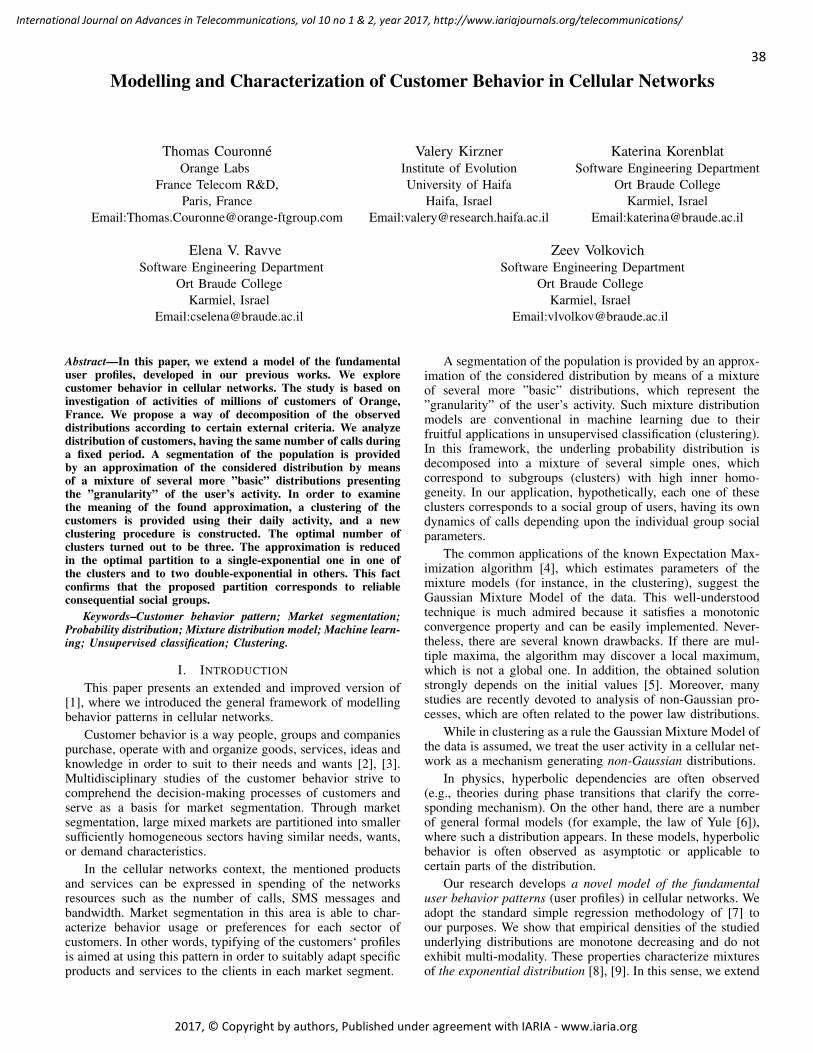
Modelling and Characterization of Customer Behavior in Cellular Networks

Thomas CouronneOrange Labs

France Telecom R&D,Paris, France

Email:[email protected]

Valery KirznerInstitute of EvolutionUniversity of Haifa

Haifa, IsraelEmail:[email protected]

Katerina KorenblatSoftware Engineering Department

Ort Braude CollegeKarmiel, Israel


Elena V. RavveSoftware Engineering Department



Zeev VolkovichSoftware Engineering Department



Abstract—In this paper, we extend a model of the fundamentaluser profiles, developed in our previous works. We explorecustomer behavior in cellular networks. The study is based oninvestigation of activities of millions of customers of Orange,France. We propose a way of decomposition of the observeddistributions according to certain external criteria. We analyzedistribution of customers, having the same number of calls duringa fixed period. A segmentation of the population is providedby an approximation of the considered distribution by meansof a mixture of several more ”basic” distributions presentingthe ”granularity” of the user’s activity. In order to examinethe meaning of the found approximation, a clustering of thecustomers is provided using their daily activity, and a newclustering procedure is constructed. The optimal number ofclusters turned out to be three. The approximation is reducedin the optimal partition to a single-exponential one in one ofthe clusters and to two double-exponential in others. This factconfirms that the proposed partition corresponds to reliableconsequential social groups.

Keywords–Customer behavior pattern; Market segmentation;Probability distribution; Mixture distribution model; Machine learn-ing; Unsupervised classification; Clustering.

I. INTRODUCTION

This paper presents an extended and improved version of[1], where we introduced the general framework of modellingbehavior patterns in cellular networks.

Customer behavior is a way people, groups and companiespurchase, operate with and organize goods, services, ideas andknowledge in order to suit to their needs and wants [2], [3].Multidisciplinary studies of the customer behavior strive tocomprehend the decision-making processes of customers andserve as a basis for market segmentation. Through marketsegmentation, large mixed markets are partitioned into smallersufficiently homogeneous sectors having similar needs, wants,or demand characteristics.

In the cellular networks context, the mentioned productsand services can be expressed in spending of the networksresources such as the number of calls, SMS messages andbandwidth. Market segmentation in this area is able to char-acterize behavior usage or preferences for each sector ofcustomers. In other words, typifying of the customers‘ profilesis aimed at using this pattern in order to suitably adapt specificproducts and services to the clients in each market segment.

A segmentation of the population is provided by an approx-imation of the considered distribution by means of a mixtureof several more ”basic” distributions, which represent the”granularity” of the user’s activity. Such mixture distributionmodels are conventional in machine learning due to theirfruitful applications in unsupervised classification (clustering).In this framework, the underling probability distribution isdecomposed into a mixture of several simple ones, whichcorrespond to subgroups (clusters) with high inner homo-geneity. In our application, hypothetically, each one of theseclusters corresponds to a social group of users, having its owndynamics of calls depending upon the individual group socialparameters.

The common applications of the known Expectation Max-imization algorithm [4], which estimates parameters of themixture models (for instance, in the clustering), suggest theGaussian Mixture Model of the data. This well-understoodtechnique is much admired because it satisfies a monotonicconvergence property and can be easily implemented. Never-theless, there are several known drawbacks. If there are mul-tiple maxima, the algorithm may discover a local maximum,which is not a global one. In addition, the obtained solutionstrongly depends on the initial values [5]. Moreover, manystudies are recently devoted to analysis of non-Gaussian pro-cesses, which are often related to the power law distributions.

While in clustering as a rule the Gaussian Mixture Model ofthe data is assumed, we treat the user activity in a cellular net-work as a mechanism generating non-Gaussian distributions.

In physics, hyperbolic dependencies are often observed(e.g., theories during phase transitions that clarify the corre-sponding mechanism). On the other hand, there are a numberof general formal models (for example, the law of Yule [6]),where such a distribution appears. In these models, hyperbolicbehavior is often observed as asymptotic or applicable tocertain parts of the distribution.

Our research develops a novel model of the fundamentaluser behavior patterns (user profiles) in cellular networks. Weadopt the standard simple regression methodology of [7] toour purposes. We show that empirical densities of the studiedunderlying distributions are monotone decreasing and do notexhibit multi-modality. These properties characterize mixturesof the exponential distribution [8], [9]. In this sense, we extend

38



the study of [10], where it was shown that a parallel useractivity in recording in an email address book leads to anappropriate exponential distribution of the clients.

In order to explore the meaning of the found approxima-tion, a clustering of the customers is provided, based on theirdaily activity, and a new clustering procedure is constructedin the spirit of the bi-clustering methodology of [11], [12].

We base our study on analysis of the underlying distributionof customers, who have the same number of calls during a fixedperiod, say a day. In this research, an exponential distributionmixture model is applied. It is shown that a three-exponentialdistribution fits well the needed target.

The estimated optimal number of clusters turned out tobe three. A straightforward clustering of the original data ishardly expected to deliver a robust and meaningful partition.Such a situation is a common place in the current practice.Moreover, in many applications the aim is to reveal not merelypotential clusters, but also a quite small number of variables,which adequately settle that partition. For instance, the sparseK-means (SK-means) proposed in [13], at once discovers theclusters and the key clustering variables.

A new procedure in the spirit of such a bi-clusteringmethodology, where features and items are simultaneouslyclustered, is applied in this paper. Firstly, 24 hours inside a day(the features) are clustered consistent with the correspondingusers’ activity. In the next step, the users are divided in groupsaccording to their occurrences in the previous partition ofhours. As a result, a sufficiently robust clustering of users isobtained together with a description of the clusters in terms ofcall activity.

The observed dissimilarity between hours (from the pointof view of the users’ behavior) can be naturally characterizedby a distance between the corresponding distributions. In thispaper, we employ Kolmogorov-Smirnov two sample test statis-tic [14], [15], which is actually the maximal distance betweentwo empirical normalized cumulative distribution functions.

Then we use the Partitioning Around Medoids clusteringalgorithm [16], in order to cluster the data. This algorithmoperates with a distance matrix, but not with the itemsthemselves. This is feasible for small data sets (such as theconsidered one, composed of 24 hours) and a small numberof clusters three in our case. One of the input parametersof the algorithm is the number of clusters. We estimate theoptimal number of their hours clusters, using the Silhouettecoefficient of [17]. Here ideas of both cohesion and separationare combined: for individual points as well as for partitions.The number of clusters was checked in the interval of [2−10],and the optimal one was found to be 3 for all the considereddata sets.

When we obtain classification of users’ activity across thehour clusters, we built a vector, composed of the fractions ofcalls falling within each hour cluster. At this stage, we produceuser clustering employing this new data representation. Notethat, due to the large amount of data, we deal here with ahigh complexity clustering task. It means that the traditionalclustering algorithms cannot be directly applied to this situa-tion. In order to resolve this problem we apply a resamplingclustering procedure, according to which the whole data set ispartitioned based on clustering of its samples.

Figure 1. DSN curves for InCalls (a) and OutCalls (b), obtained oneach day of the whole period of observation (13 days).

Finally, we obtain the optimal partition with a single-exponential call distribution in one of the clusters and twodouble-exponential call distributions in others. This fact con-firms that the proposed partition corresponds to reliable con-sequential social groups. We emphasize the fact that thesimilarity measure, applied in the clustering process, is formedwithout any reference to the previously discussed mixturemodel.

The results, presented in the paper, are obtained by meansof a study of the daily activity of a real group of users duringthe period from March 31, 2009 through April 11, 2009. Foreach considered day, several million users in this group areactive (making one or more calls). The time of each input oroutput call is known. Note that the sets of active users ondifferent days vary.

The paper is structured as follows. Section II is devotedto a distribution model of user activity and its decomposition.Section III describes the customer clustering procedure and itsevaluations. The section presents model-based evaluation ofthe proposed customer classification. Section IV summarizesthe paper and provides outlook.

II. DISTRIBUTION MODEL OF USER ACTIVITY

In this section, we consider a mixture model approximationof the underlying distribution of users having the same numberof calls during a day. We denote by DSN the Day SameNumber distribution. We distinguish two types of user activity:input calls, denoted by InCalls, and output calls, denoted byOutCalls.

All users (about five millions) are divided into groupsaccording to their number of calls per day, so that the i-th group contains all customers having exactly i calls per aparticular day. The size of the i-th group is denoted by Ni.Obviously, the contents and sizes of the groups are not thesame for different days. In addition, the number of groups withi > 100 is very small in the dataset, and these groups mostlikely contain ”non-standard” users such that sales agents, callcenters and so on. We omit such groups together with users,who do not call at all in a given day, since this lack of activitycould be explained by factors that are not directly related tothe user activity on the network.

The DSN curves, normalized to 1, of InCalls (a) andOutCalls (b) as well as the corresponding numbers of callsranging from 1 to 50, are shown in Fig. 1. We note that thecurves are of almost the same monotonically decreasing formfor all 13 days of the observation.

39



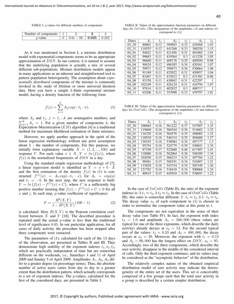
TABLE I. p-values for different numbers of components

Number of components 1 2 3 4p-value 0 8.6e− 06 0.025 0.282

As it was mentioned in Section I, a mixture distributionmodel with exponential components seems to be an appropriateapproximation of DSN . In our context, it is natural to assumethat the underlying population is actually a mix of severaldifferent sub-populations. Mixture distribution models appearin many applications as an inherent and straightforward tool topattern population heterogeneity. The assumption about expo-nentially distributed components of the mixture is commonlyinvoked in the study of lifetime or more universal durationdata. Here you have a simple k-finite exponential mixturemodel, having a density function of the following form

f(x) =

k∑j=1

Ajexp(−tj · x), (1)

where Aj and tj , j = 1, ...k are nonnegative numbers, and∑kj=1Aj = 1. For a given number of components k, the

Expectation–Maximization (EM ) algorithm [4] is a traditionalmethod for maximum likelihood estimation of finite mixtures.

However, we apply another approach in the spirit of thelinear regression methodology without any prior assumptionabout k - the number of components. For this purpose, weinitially form explanatory variable X = (1, 2, ..., 100) andresponse Y . For each value x ∈ X , Y = ln (f(x)), wheref(x) is the normalized frequencies of DSN in a day.

Using the standard simple regression methodology of [7],a linear regression model is identified as Y = a + b · Xand the first estimation of the density f(x) in (1) is con-structed: f (1)(x) = A1 exp(−t1 · x), for A1 = exp(a)and t1 = −b. In the next step, the new response is built:Y = ln

(f(x)− f (1)(x) + C

), where C is a sufficiently big

positive number insuring that f(x)− f (1)(x) + C > 0 for allx and j. In each step, p-value coefficient of significance:

F =R2(X,Y )

1−R2(X,Y )(100− 1) (2)

is calculated. Here R(X,Y ) is the Pearson correlation coef-ficient between X and Y [18]. The described procedure isrepeated until the actual p-value is less than the traditionallevel of significance 0.05. In our particular application, for allcases of daily activity, the procedure has been stopped afterthree components were extracted.

The parameters of (1), calculated for each of the 13 daysof the observation, are presented in Tables II and III. Theydemonstrate high stability of the exponent indexes t1, t2, t3,which are practically independent of time but are somewhatdifferent on the weekends, i.e., Saturdays 4 and 11 of April2009 and Sunday 5 of April 2009. Amplitudes A1, A2, A3 dif-fer to a greater degree (in percentage terms). Thus, the absolutenumber of active users varies from day to day to a greaterextent than the distribution pattern, which actually correspondsto a set of exponent indexes. The p-values, calculated for thefirst of the considered days, are presented in Table I.

TABLE II. Values of the approximation function parameters on differentdays for InCalls. (The designations of the amplitudes (A) and indexes (t)

correspond to (1))

Dates A1 t1 A2 t2 A3 t303 30 80001 0.12 399893 0.32 420568 1.0203 31 110555 0.12 441268 0.33 380258 1.1504 01 94021 0.11 421456 0.31 401002 1.0104 02 99683 0.11 419564 0.3 411258 1.0504 03 96660 0.11 409176 0.29 405050 0.9804 04 90424 0.12 406385 0.34 420161 1.0704 05 59971 0.12 399873 0.36 530064 1.0804 06 91189 0.11 425022 0.31 450957 1.0404 07 83467 0.11 415012 0.3 431301 0.9604 08 93358 0.11 430842 0.31 422297 104 09 102169 0.11 426124 0.31 416794 1.0704 10 97814 0.11 402832 0.3 408717 104 11 65206 0.11 353998 0.33 439797 1.01

TABLE III. Values of the approximation function parameters on differentdays for OutCalls. (The designations of the amplitudes (A) and indexes (t)

correspond to (1))

Dates A1 t1 A2 t2 A3 t303 30 100684 0.16 561222 0.37 527907 1.2503 31 119660 0.16 560344 0.36 514682 1.3204 01 116329 0.16 564578 0.35 498085 1.3204 02 118910 0.16 546314 0.35 494688 1.2704 03 130193 0.16 538984 0.34 497177 1.304 04 95354 0.16 524779 0.39 548041 1.3404 05 87109 0.17 522660 0.46 617407 1.4104 06 110086 0.16 562064 0.36 548389 1.3404 07 102030 0.15 560233 0.35 497784 1.2204 08 90481 0.15 568191 0.34 510487 1.2104 09 115820 0.16 543334 0.34 505349 1.2604 10 121782 0.16 518418 0.34 500068 1.2404 11 80915 0.15 445910 0.39 538691 1.22

In the case of InCalls (Table II), the ratio of the exponentindexes is: 3·t1 ≈ t2, 3·t2 ≈ t3. In the case of OutCalls (TableIII), this ratio is somewhat different: 2 · t1 ≈ t2, 3.5 · t2 ≈ t3.The decay value x0 of each component in (1) is chosen inorder to normalize the component value at this point to 1.

The components are not equivalent in the sense of theirdecay value (see Table IV). In fact, the exponent with indext3 = 1.0 and amplitude A3 = 500, 000 (these values aretypical for one of the three exponents, which describe the dailyactivity) already decays at x0 = 13. For the second typicalpair of the values: t2 = 0.33 and A2 = 400, 000, the decayoccurs at x0 = 39. Moreover, the exponent with t1 = 0.12and A1 = 90, 000 has the longest effect on DSN : x0 = 95.Accordingly, two of the three components, which describe theuser activity, disappear in the middle of the considered intervalof calls. Only the third exponent continues, and its values maybe considered as the ”asymptotic behavior” of the distribution.

The relatively complex nature of the obtained empiricaldistribution model of user activity may indicate the hetero-geneity of the entire set of the users. This set is conceivablycomposed of a few groups such that the total user activity ina group is described by a certain simpler distribution.

40



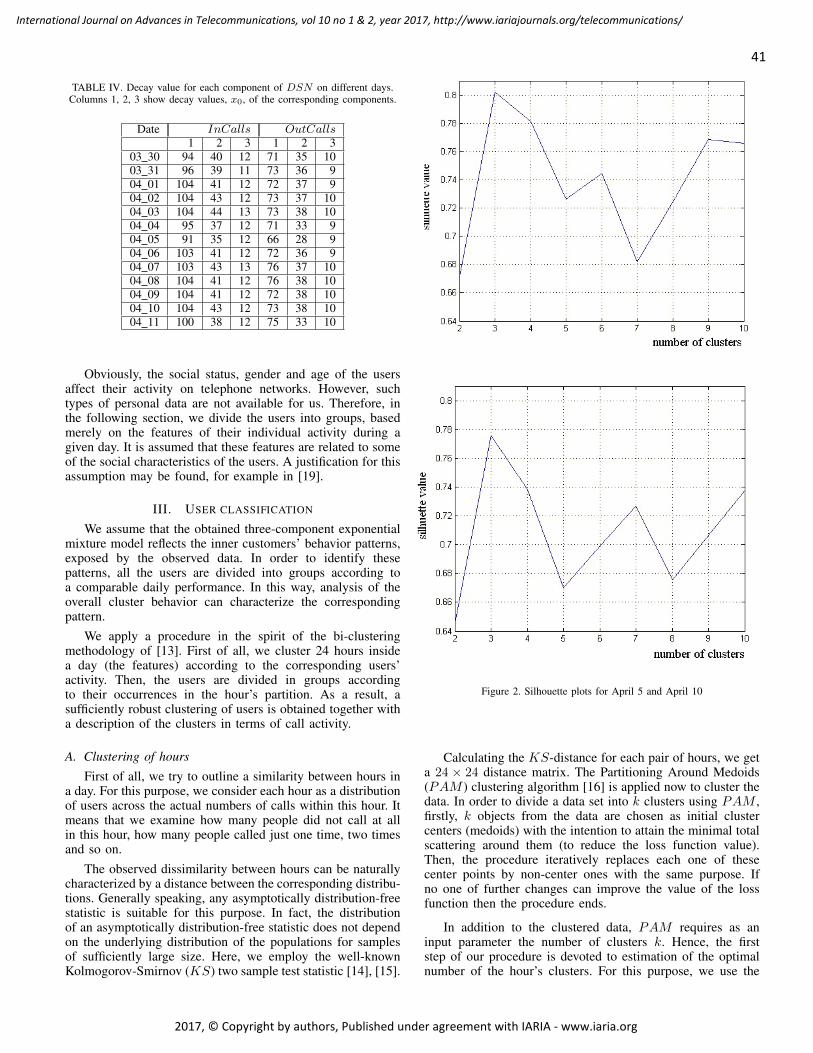
TABLE IV. Decay value for each component of DSN on different days.Columns 1, 2, 3 show decay values, x0, of the corresponding components.

Date InCalls OutCalls1 2 3 1 2 3

03 30 94 40 12 71 35 1003 31 96 39 11 73 36 904 01 104 41 12 72 37 904 02 104 43 12 73 37 1004 03 104 44 13 73 38 1004 04 95 37 12 71 33 904 05 91 35 12 66 28 904 06 103 41 12 72 36 904 07 103 43 13 76 37 1004 08 104 41 12 76 38 1004 09 104 41 12 72 38 1004 10 104 43 12 73 38 1004 11 100 38 12 75 33 10

Obviously, the social status, gender and age of the usersaffect their activity on telephone networks. However, suchtypes of personal data are not available for us. Therefore, inthe following section, we divide the users into groups, basedmerely on the features of their individual activity during agiven day. It is assumed that these features are related to someof the social characteristics of the users. A justification for thisassumption may be found, for example in [19].

III. USER CLASSIFICATION

We assume that the obtained three-component exponentialmixture model reflects the inner customers’ behavior patterns,exposed by the observed data. In order to identify thesepatterns, all the users are divided into groups according toa comparable daily performance. In this way, analysis of theoverall cluster behavior can characterize the correspondingpattern.

We apply a procedure in the spirit of the bi-clusteringmethodology of [13]. First of all, we cluster 24 hours insidea day (the features) according to the corresponding users’activity. Then, the users are divided in groups accordingto their occurrences in the hour’s partition. As a result, asufficiently robust clustering of users is obtained together witha description of the clusters in terms of call activity.

A. Clustering of hours

First of all, we try to outline a similarity between hours ina day. For this purpose, we consider each hour as a distributionof users across the actual numbers of calls within this hour. Itmeans that we examine how many people did not call at allin this hour, how many people called just one time, two timesand so on.

The observed dissimilarity between hours can be naturallycharacterized by a distance between the corresponding distribu-tions. Generally speaking, any asymptotically distribution-freestatistic is suitable for this purpose. In fact, the distributionof an asymptotically distribution-free statistic does not dependon the underlying distribution of the populations for samplesof sufficiently large size. Here, we employ the well-knownKolmogorov-Smirnov (KS) two sample test statistic [14], [15].

Figure 2. Silhouette plots for April 5 and April 10

Calculating the KS-distance for each pair of hours, we geta 24 × 24 distance matrix. The Partitioning Around Medoids(PAM ) clustering algorithm [16] is applied now to cluster thedata. In order to divide a data set into k clusters using PAM ,firstly, k objects from the data are chosen as initial clustercenters (medoids) with the intention to attain the minimal totalscattering around them (to reduce the loss function value).Then, the procedure iteratively replaces each one of thesecenter points by non-center ones with the same purpose. Ifno one of further changes can improve the value of the lossfunction then the procedure ends.

In addition to the clustered data, PAM requires as aninput parameter the number of clusters k. Hence, the firststep of our procedure is devoted to estimation of the optimalnumber of the hour’s clusters. For this purpose, we use the

41



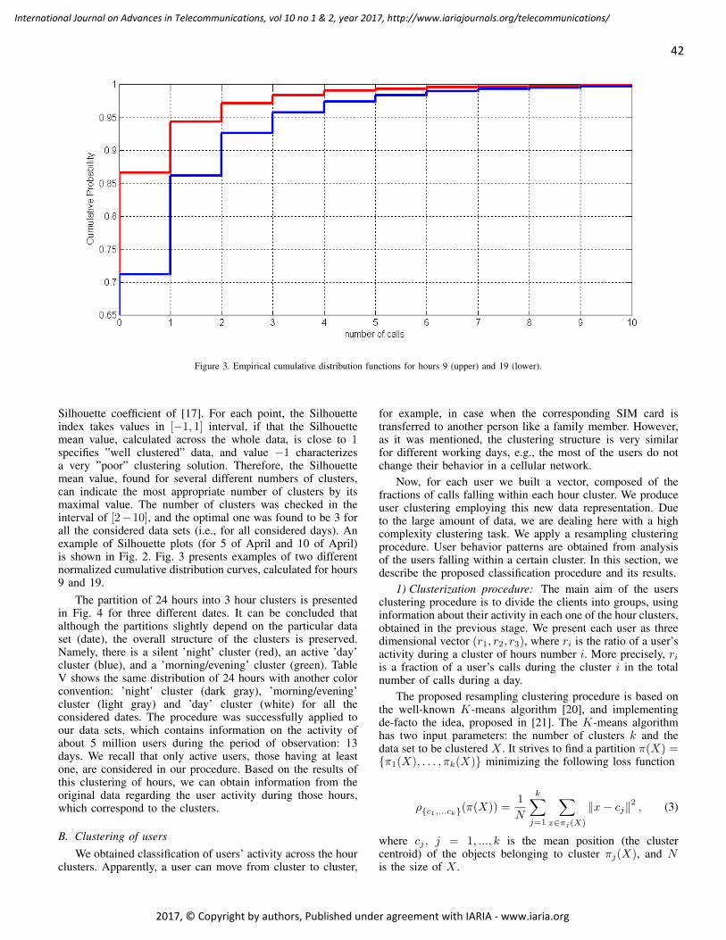
Figure 3. Empirical cumulative distribution functions for hours 9 (upper) and 19 (lower).

Silhouette coefficient of [17]. For each point, the Silhouetteindex takes values in [−1, 1] interval, if that the Silhouettemean value, calculated across the whole data, is close to 1specifies ”well clustered” data, and value −1 characterizesa very ”poor” clustering solution. Therefore, the Silhouettemean value, found for several different numbers of clusters,can indicate the most appropriate number of clusters by itsmaximal value. The number of clusters was checked in theinterval of [2−10], and the optimal one was found to be 3 forall the considered data sets (i.e., for all considered days). Anexample of Silhouette plots (for 5 of April and 10 of April)is shown in Fig. 2. Fig. 3 presents examples of two differentnormalized cumulative distribution curves, calculated for hours9 and 19.

The partition of 24 hours into 3 hour clusters is presentedin Fig. 4 for three different dates. It can be concluded thatalthough the partitions slightly depend on the particular dataset (date), the overall structure of the clusters is preserved.Namely, there is a silent ’night’ cluster (red), an active ’day’cluster (blue), and a ’morning/evening’ cluster (green). TableV shows the same distribution of 24 hours with another colorconvention: ’night’ cluster (dark gray), ’morning/evening’cluster (light gray) and ’day’ cluster (white) for all theconsidered dates. The procedure was successfully applied toour data sets, which contains information on the activity ofabout 5 million users during the period of observation: 13days. We recall that only active users, those having at leastone, are considered in our procedure. Based on the results ofthis clustering of hours, we can obtain information from theoriginal data regarding the user activity during those hours,which correspond to the clusters.

B. Clustering of usersWe obtained classification of users’ activity across the hour

clusters. Apparently, a user can move from cluster to cluster,

for example, in case when the corresponding SIM card istransferred to another person like a family member. However,as it was mentioned, the clustering structure is very similarfor different working days, e.g., the most of the users do notchange their behavior in a cellular network.

Now, for each user we built a vector, composed of thefractions of calls falling within each hour cluster. We produceuser clustering employing this new data representation. Dueto the large amount of data, we are dealing here with a highcomplexity clustering task. We apply a resampling clusteringprocedure. User behavior patterns are obtained from analysisof the users falling within a certain cluster. In this section, wedescribe the proposed classification procedure and its results.

1) Clusterization procedure: The main aim of the usersclustering procedure is to divide the clients into groups, usinginformation about their activity in each one of the hour clusters,obtained in the previous stage. We present each user as threedimensional vector (r1, r2, r3), where ri is the ratio of a user’sactivity during a cluster of hours number i. More precisely, riis a fraction of a user’s calls during the cluster i in the totalnumber of calls during a day.

The proposed resampling clustering procedure is based onthe well-known K-means algorithm [20], and implementingde-facto the idea, proposed in [21]. The K-means algorithmhas two input parameters: the number of clusters k and thedata set to be clustered X . It strives to find a partition π(X) ={π1(X), . . . , πk(X)} minimizing the following loss function

ρ{c1,...ck}(π(X)) =1

N

k∑j=1

∑x∈πj(X)

‖x− cj‖2 , (3)

where cj , j = 1, ..., k is the mean position (the clustercentroid) of the objects belonging to cluster πj(X), and Nis the size of X .

42



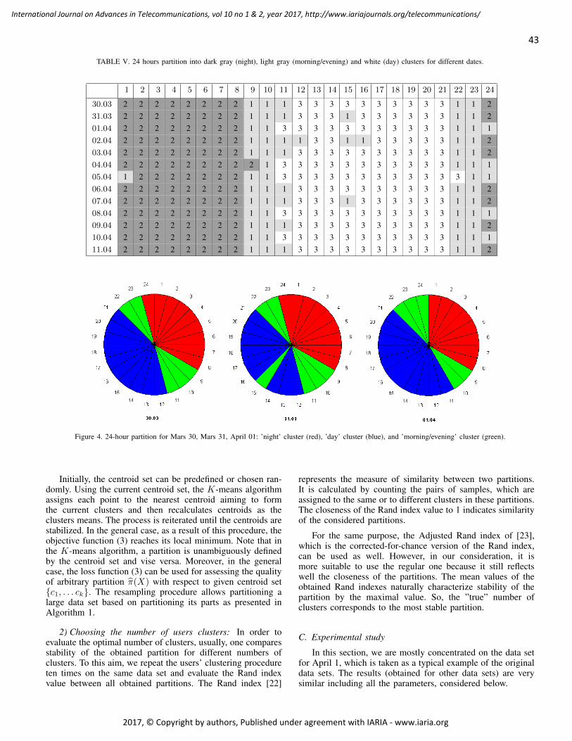
TABLE V. 24 hours partition into dark gray (night), light gray (morning/evening) and white (day) clusters for different dates.

1 2 3 4 5 6 7 8 9 10 11 12 13 14 15 16 17 18 19 20 21 22 23 24

30.03 2 2 2 2 2 2 2 2 1 1 1 3 3 3 3 3 3 3 3 3 3 1 1 231.03 2 2 2 2 2 2 2 2 1 1 1 3 3 3 1 3 3 3 3 3 3 1 1 201.04 2 2 2 2 2 2 2 2 1 1 3 3 3 3 3 3 3 3 3 3 3 1 1 102.04 2 2 2 2 2 2 2 2 1 1 1 1 3 3 1 1 3 3 3 3 3 1 1 203.04 2 2 2 2 2 2 2 2 1 1 1 3 3 3 3 3 3 3 3 3 3 1 1 204.04 2 2 2 2 2 2 2 2 2 1 3 3 3 3 3 3 3 3 3 3 3 1 1 105.04 1 2 2 2 2 2 2 2 1 1 3 3 3 3 3 3 3 3 3 3 3 3 1 106.04 2 2 2 2 2 2 2 2 1 1 1 3 3 3 3 3 3 3 3 3 3 1 1 207.04 2 2 2 2 2 2 2 2 1 1 1 3 3 3 1 3 3 3 3 3 3 1 1 208.04 2 2 2 2 2 2 2 2 1 1 3 3 3 3 3 3 3 3 3 3 3 1 1 109.04 2 2 2 2 2 2 2 2 1 1 1 3 3 3 3 3 3 3 3 3 3 1 1 210.04 2 2 2 2 2 2 2 2 1 1 3 3 3 3 3 3 3 3 3 3 3 1 1 111.04 2 2 2 2 2 2 2 2 1 1 1 3 3 3 3 3 3 3 3 3 3 1 1 2

Figure 4. 24-hour partition for Mars 30, Mars 31, April 01: ’night’ cluster (red), ’day’ cluster (blue), and ’morning/evening’ cluster (green).

Initially, the centroid set can be predefined or chosen ran-domly. Using the current centroid set, the K-means algorithmassigns each point to the nearest centroid aiming to formthe current clusters and then recalculates centroids as theclusters means. The process is reiterated until the centroids arestabilized. In the general case, as a result of this procedure, theobjective function (3) reaches its local minimum. Note that inthe K-means algorithm, a partition is unambiguously definedby the centroid set and vise versa. Moreover, in the generalcase, the loss function (3) can be used for assessing the qualityof arbitrary partition π(X) with respect to given centroid set{c1, . . . ck}. The resampling procedure allows partitioning alarge data set based on partitioning its parts as presented inAlgorithm 1.

2) Choosing the number of users clusters: In order toevaluate the optimal number of clusters, usually, one comparesstability of the obtained partition for different numbers ofclusters. To this aim, we repeat the users’ clustering procedureten times on the same data set and evaluate the Rand indexvalue between all obtained partitions. The Rand index [22]

represents the measure of similarity between two partitions.It is calculated by counting the pairs of samples, which areassigned to the same or to different clusters in these partitions.The closeness of the Rand index value to 1 indicates similarityof the considered partitions.

For the same purpose, the Adjusted Rand index of [23],which is the corrected-for-chance version of the Rand index,can be used as well. However, in our consideration, it ismore suitable to use the regular one because it still reflectswell the closeness of the partitions. The mean values of theobtained Rand indexes naturally characterize stability of thepartition by the maximal value. So, the ”true” number ofclusters corresponds to the most stable partition.

C. Experimental study

In this section, we are mostly concentrated on the data setfor April 1, which is taken as a typical example of the originaldata sets. The results (obtained for other data sets) are verysimilar including all the parameters, considered below.

43



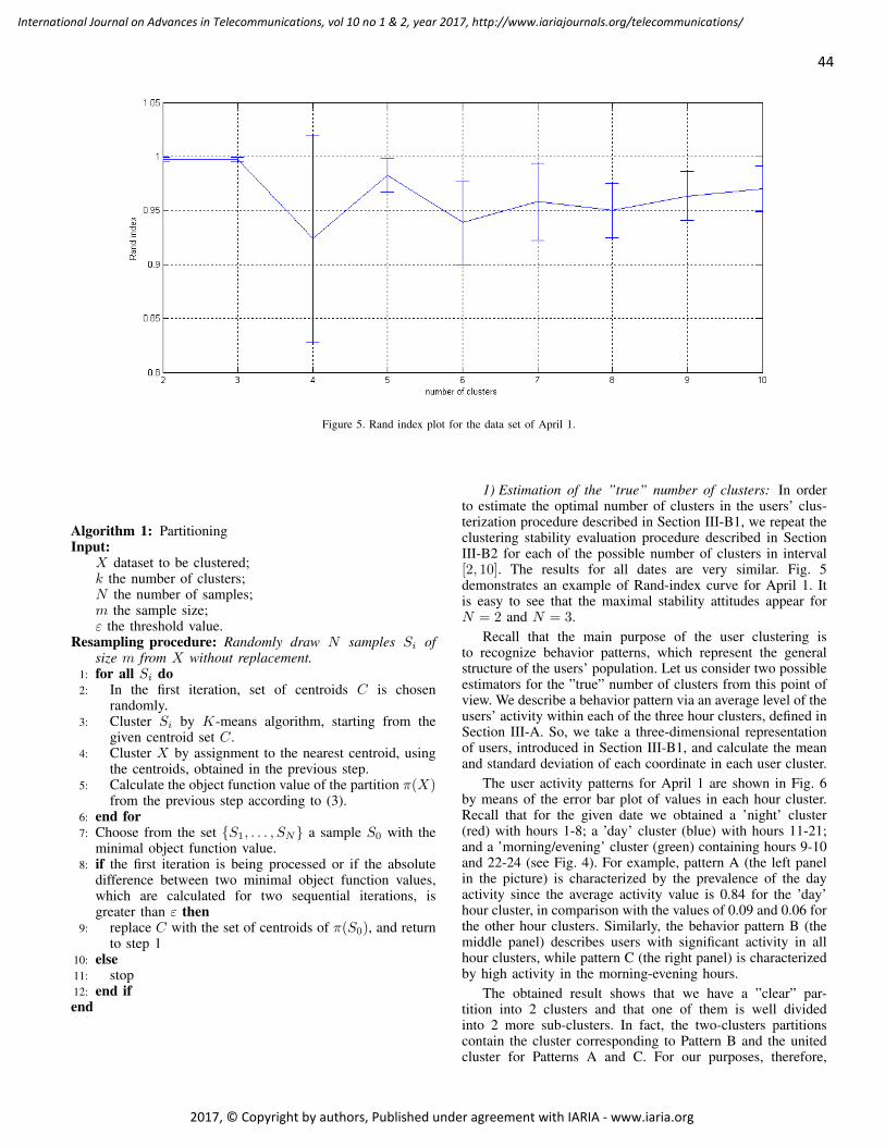
Figure 5. Rand index plot for the data set of April 1.

Algorithm 1: PartitioningInput:

X dataset to be clustered;k the number of clusters;N the number of samples;m the sample size;ε the threshold value.

Resampling procedure: Randomly draw N samples Si ofsize m from X without replacement.

1: for all Si do2: In the first iteration, set of centroids C is chosen

randomly.3: Cluster Si by K-means algorithm, starting from the

given centroid set C.4: Cluster X by assignment to the nearest centroid, using

the centroids, obtained in the previous step.5: Calculate the object function value of the partition π(X)

from the previous step according to (3).6: end for7: Choose from the set {S1, . . . , SN} a sample S0 with the

minimal object function value.8: if the first iteration is being processed or if the absolute

difference between two minimal object function values,which are calculated for two sequential iterations, isgreater than ε then

9: replace C with the set of centroids of π(S0), and returnto step 1

10: else11: stop12: end ifend

1) Estimation of the ”true” number of clusters: In orderto estimate the optimal number of clusters in the users’ clus-terization procedure described in Section III-B1, we repeat theclustering stability evaluation procedure described in SectionIII-B2 for each of the possible number of clusters in interval[2, 10]. The results for all dates are very similar. Fig. 5demonstrates an example of Rand-index curve for April 1. Itis easy to see that the maximal stability attitudes appear forN = 2 and N = 3.

Recall that the main purpose of the user clustering isto recognize behavior patterns, which represent the generalstructure of the users’ population. Let us consider two possibleestimators for the ”true” number of clusters from this point ofview. We describe a behavior pattern via an average level of theusers’ activity within each of the three hour clusters, defined inSection III-A. So, we take a three-dimensional representationof users, introduced in Section III-B1, and calculate the meanand standard deviation of each coordinate in each user cluster.

The user activity patterns for April 1 are shown in Fig. 6by means of the error bar plot of values in each hour cluster.Recall that for the given date we obtained a ’night’ cluster(red) with hours 1-8; a ’day’ cluster (blue) with hours 11-21;and a ’morning/evening’ cluster (green) containing hours 9-10and 22-24 (see Fig. 4). For example, pattern A (the left panelin the picture) is characterized by the prevalence of the dayactivity since the average activity value is 0.84 for the ’day’hour cluster, in comparison with the values of 0.09 and 0.06 forthe other hour clusters. Similarly, the behavior pattern B (themiddle panel) describes users with significant activity in allhour clusters, while pattern C (the right panel) is characterizedby high activity in the morning-evening hours.

The obtained result shows that we have a ”clear” par-tition into 2 clusters and that one of them is well dividedinto 2 more sub-clusters. In fact, the two-clusters partitionscontain the cluster corresponding to Pattern B and the unitedcluster for Patterns A and C. For our purposes, therefore,

44



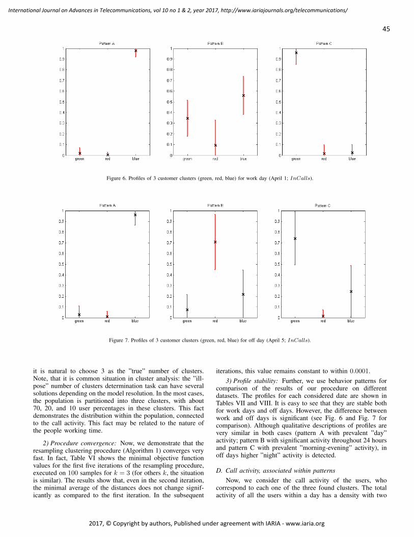
Figure 6. Profiles of 3 customer clusters (green, red, blue) for work day (April 1; InCalls).

Figure 7. Profiles of 3 customer clusters (green, red, blue) for off day (April 5; InCalls).

it is natural to choose 3 as the ”true” number of clusters.Note, that it is common situation in cluster analysis: the ”ill-pose” number of clusters determination task can have severalsolutions depending on the model resolution. In the most cases,the population is partitioned into three clusters, with about70, 20, and 10 user percentages in these clusters. This factdemonstrates the distribution within the population, connectedto the call activity. This fact may be related to the nature ofthe people working time.

2) Procedure convergence: Now, we demonstrate that theresampling clustering procedure (Algorithm 1) converges veryfast. In fact, Table VI shows the minimal objective functionvalues for the first five iterations of the resampling procedure,executed on 100 samples for k = 3 (for others k, the situationis similar). The results show that, even in the second iteration,the minimal average of the distances does not change signif-icantly as compared to the first iteration. In the subsequent

iterations, this value remains constant to within 0.0001.3) Profile stability: Further, we use behavior patterns for

comparison of the results of our procedure on differentdatasets. The profiles for each considered date are shown inTables VII and VIII. It is easy to see that they are stable bothfor work days and off days. However, the difference betweenwork and off days is significant (see Fig. 6 and Fig. 7 forcomparison). Although qualitative descriptions of profiles arevery similar in both cases (pattern A with prevalent ”day”activity; pattern B with significant activity throughout 24 hoursand pattern C with prevalent ”morning-evening” activity), inoff days higher ”night” activity is detected.

D. Call activity, associated within patternsNow, we consider the call activity of the users, who

correspond to each one of the three found clusters. The totalactivity of all the users within a day has a density with two

45



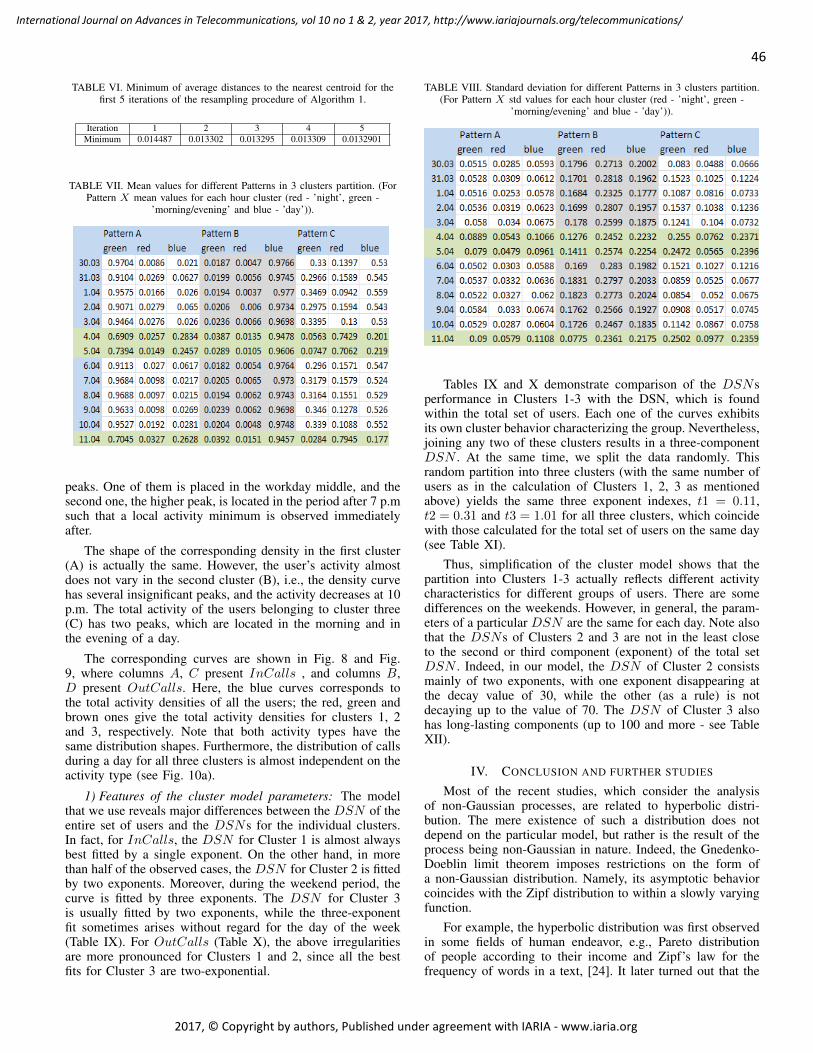
TABLE VI. Minimum of average distances to the nearest centroid for thefirst 5 iterations of the resampling procedure of Algorithm 1.

Iteration 1 2 3 4 5Minimum 0.014487 0.013302 0.013295 0.013309 0.0132901

TABLE VII. Mean values for different Patterns in 3 clusters partition. (ForPattern X mean values for each hour cluster (red - ’night’, green -

’morning/evening’ and blue - ’day’)).

peaks. One of them is placed in the workday middle, and thesecond one, the higher peak, is located in the period after 7 p.msuch that a local activity minimum is observed immediatelyafter.

The shape of the corresponding density in the first cluster(A) is actually the same. However, the user’s activity almostdoes not vary in the second cluster (B), i.e., the density curvehas several insignificant peaks, and the activity decreases at 10p.m. The total activity of the users belonging to cluster three(C) has two peaks, which are located in the morning and inthe evening of a day.

The corresponding curves are shown in Fig. 8 and Fig.9, where columns A, C present InCalls , and columns B,D present OutCalls. Here, the blue curves corresponds tothe total activity densities of all the users; the red, green andbrown ones give the total activity densities for clusters 1, 2and 3, respectively. Note that both activity types have thesame distribution shapes. Furthermore, the distribution of callsduring a day for all three clusters is almost independent on theactivity type (see Fig. 10a).

1) Features of the cluster model parameters: The modelthat we use reveals major differences between the DSN of theentire set of users and the DSNs for the individual clusters.In fact, for InCalls, the DSN for Cluster 1 is almost alwaysbest fitted by a single exponent. On the other hand, in morethan half of the observed cases, the DSN for Cluster 2 is fittedby two exponents. Moreover, during the weekend period, thecurve is fitted by three exponents. The DSN for Cluster 3is usually fitted by two exponents, while the three-exponentfit sometimes arises without regard for the day of the week(Table IX). For OutCalls (Table X), the above irregularitiesare more pronounced for Clusters 1 and 2, since all the bestfits for Cluster 3 are two-exponential.

TABLE VIII. Standard deviation for different Patterns in 3 clusters partition.(For Pattern X std values for each hour cluster (red - ’night’, green -

’morning/evening’ and blue - ’day’)).

Tables IX and X demonstrate comparison of the DSNsperformance in Clusters 1-3 with the DSN, which is foundwithin the total set of users. Each one of the curves exhibitsits own cluster behavior characterizing the group. Nevertheless,joining any two of these clusters results in a three-componentDSN . At the same time, we split the data randomly. Thisrandom partition into three clusters (with the same number ofusers as in the calculation of Clusters 1, 2, 3 as mentionedabove) yields the same three exponent indexes, t1 = 0.11,t2 = 0.31 and t3 = 1.01 for all three clusters, which coincidewith those calculated for the total set of users on the same day(see Table XI).

Thus, simplification of the cluster model shows that thepartition into Clusters 1-3 actually reflects different activitycharacteristics for different groups of users. There are somedifferences on the weekends. However, in general, the param-eters of a particular DSN are the same for each day. Note alsothat the DSNs of Clusters 2 and 3 are not in the least closeto the second or third component (exponent) of the total setDSN . Indeed, in our model, the DSN of Cluster 2 consistsmainly of two exponents, with one exponent disappearing atthe decay value of 30, while the other (as a rule) is notdecaying up to the value of 70. The DSN of Cluster 3 alsohas long-lasting components (up to 100 and more - see TableXII).

IV. CONCLUSION AND FURTHER STUDIES

Most of the recent studies, which consider the analysisof non-Gaussian processes, are related to hyperbolic distri-bution. The mere existence of such a distribution does notdepend on the particular model, but rather is the result of theprocess being non-Gaussian in nature. Indeed, the Gnedenko-Doeblin limit theorem imposes restrictions on the form ofa non-Gaussian distribution. Namely, its asymptotic behaviorcoincides with the Zipf distribution to within a slowly varyingfunction.

For example, the hyperbolic distribution was first observedin some fields of human endeavor, e.g., Pareto distributionof people according to their income and Zipf’s law for thefrequency of words in a text, [24]. It later turned out that the

46



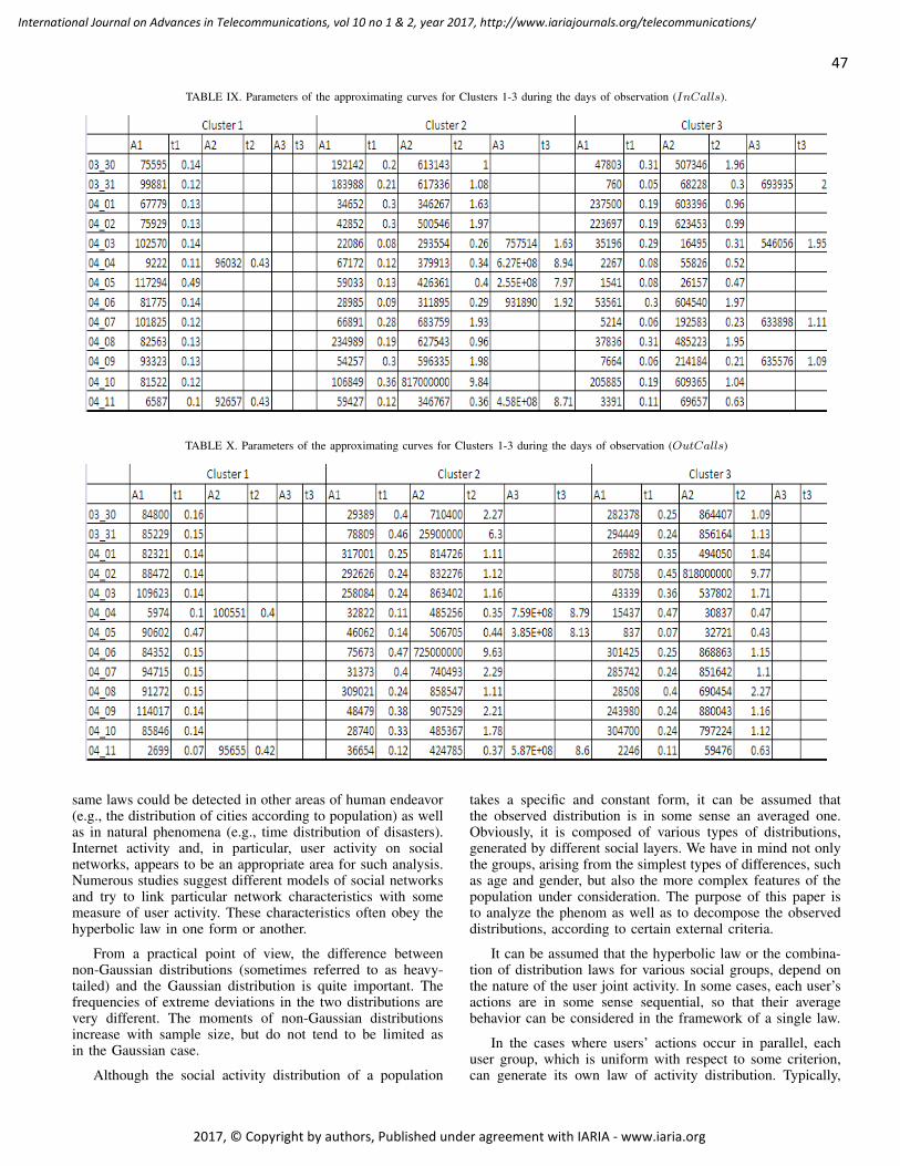
TABLE IX. Parameters of the approximating curves for Clusters 1-3 during the days of observation (InCalls).

TABLE X. Parameters of the approximating curves for Clusters 1-3 during the days of observation (OutCalls)

same laws could be detected in other areas of human endeavor(e.g., the distribution of cities according to population) as wellas in natural phenomena (e.g., time distribution of disasters).Internet activity and, in particular, user activity on socialnetworks, appears to be an appropriate area for such analysis.Numerous studies suggest different models of social networksand try to link particular network characteristics with somemeasure of user activity. These characteristics often obey thehyperbolic law in one form or another.

From a practical point of view, the difference betweennon-Gaussian distributions (sometimes referred to as heavy-tailed) and the Gaussian distribution is quite important. Thefrequencies of extreme deviations in the two distributions arevery different. The moments of non-Gaussian distributionsincrease with sample size, but do not tend to be limited asin the Gaussian case.

Although the social activity distribution of a population

takes a specific and constant form, it can be assumed thatthe observed distribution is in some sense an averaged one.Obviously, it is composed of various types of distributions,generated by different social layers. We have in mind not onlythe groups, arising from the simplest types of differences, suchas age and gender, but also the more complex features of thepopulation under consideration. The purpose of this paper isto analyze the phenom as well as to decompose the observeddistributions, according to certain external criteria.

It can be assumed that the hyperbolic law or the combina-tion of distribution laws for various social groups, depend onthe nature of the user joint activity. In some cases, each user’sactions are in some sense sequential, so that their averagebehavior can be considered in the framework of a single law.

In the cases where users’ actions occur in parallel, eachuser group, which is uniform with respect to some criterion,can generate its own law of activity distribution. Typically,

47



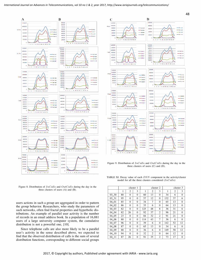
Figure 8. Distribution of InCalls and OutCalls during the day in thethree clusters of users (A) and (B).

users actions in such a group are aggregated in order to patternthe group behavior. Researchers, who study the parameters ofsuch networks, often find fractal properties and hyperbolic dis-tributions. An example of parallel user activity is the numberof records in an email address book. In a population of 16,881users of a large university computer system, the cumulativedistribution is not a powerful one, [10].

Since telephone calls are also more likely to be a paralleluser’s activity in the sense described above, we expected tofind that the observed distribution of calls is the sum of severaldistribution functions, corresponding to different social groups

Figure 9. Distribution of InCalls and OutCalls during the day in thethree clusters of users (C) and (D).

TABLE XI. Decay value of each DSN component in the activity/clustermodel for all the three clusters considered (InCalls)

cluster 1 cluster 2 cluster 31 2 3 1 2 3 1 2 3

03 30 80 0 0 60 13 0 34 6 003 31 95 0 0 57 12 0 132 37 604 01 85 0 0 34 7 0 65 13 004 02 86 0 0 35 6 0 64 13 004 03 82 0 0 125 48 8 36 31 604 04 82 26 0 92 37 2 96 21 004 05 23 0 0 84 32 2 91 21 004 06 80 0 0 114 43 7 36 6 004 07 96 0 0 39 6 0 142 52 1204 08 87 0 0 65 13 0 34 6 004 09 88 0 0 36 6 0 149 58 1204 10 94 0 0 32 2 0 64 12 004 11 87 26 0 91 35 2 73 17 0

48



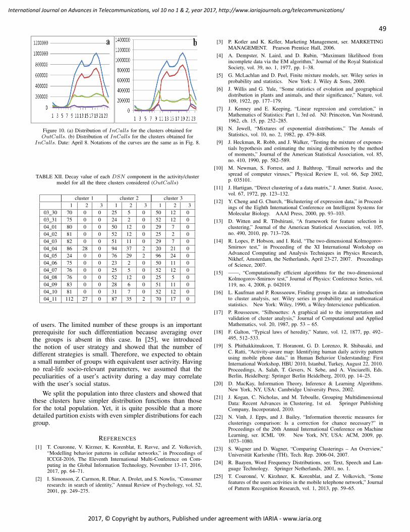
Figure 10. (a) Distribution of InCalls for the clusters obtained forOutCalls. (b) Distribution of InCalls for the clusters obtained for

InCalls. Date: April 8. Notations of the curves are the same as in Fig. 8.

TABLE XII. Decay value of each DSN component in the activity/clustermodel for all the three clusters considered (OutCalls)

cluster 1 cluster 2 cluster 31 2 3 1 2 3 1 2 3

03 30 70 0 0 25 5 0 50 12 003 31 75 0 0 24 2 0 52 12 004 01 80 0 0 50 12 0 29 7 004 02 81 0 0 52 12 0 25 2 004 03 82 0 0 51 11 0 29 7 004 04 86 28 0 94 37 2 20 21 004 05 24 0 0 76 29 2 96 24 004 06 75 0 0 23 2 0 50 11 004 07 76 0 0 25 5 0 52 12 004 08 76 0 0 52 12 0 25 5 004 09 83 0 0 28 6 0 51 11 004 10 81 0 0 31 7 0 52 12 004 11 112 27 0 87 35 2 70 17 0

of users. The limited number of these groups is an importantprerequisite for such differentiation because averaging overthe groups is absent in this case. In [25], we introducedthe notion of user strategy and showed that the number ofdifferent strategies is small. Therefore, we expected to obtaina small number of groups with equivalent user activity. Havingno real-life socio-relevant parameters, we assumed that thepeculiarities of a user’s activity during a day may correlatewith the user’s social status.

We split the population into three clusters and showed thatthese clusters have simpler distribution functions than thosefor the total population. Yet, it is quite possible that a moredetailed partition exists with even simpler distributions for eachgroup.

REFERENCES

[1] T. Couronne, V. Kirzner, K. Korenblat, E. Ravve, and Z. Volkovich,“Modelling behavior patterns in cellular networks,” in Proceedings ofICCGI-2016, The Eleventh International Multi-Conference on Com-puting in the Global Information Technology, November 13-17, 2016,2017, pp. 64–71.

[2] I. Simonson, Z. Carmon, R. Dhar, A. Drolet, and S. Nowlis, “Consumerresearch: in search of identity,” Annual Review of Psychology, vol. 52,2001, pp. 249–275.

[3] P. Kotler and K. Keller, Marketing Management, ser. MARKETINGMANAGEMENT. Pearson Prentice Hall, 2006.

[4] A. Dempster, N. Laird, and D. Rubin, “Maximum likelihood fromincomplete data via the EM algorithm,” Journal of the Royal StatisticalSociety, vol. 39, no. 1, 1977, pp. 1–38.

[5] G. McLachlan and D. Peel, Finite mixture models, ser. Wiley series inprobability and statistics. New York: J. Wiley & Sons, 2000.

[6] J. Willis and G. Yule, “Some statistics of evolution and geographicaldistribution in plants and animals, and their significance,” Nature, vol.109, 1922, pp. 177–179.

[7] J. Kenney and E. Keeping, “Linear regression and correlation,” inMathematics of Statistics: Part 1, 3rd ed. NJ: Princeton, Van Nostrand,1962, ch. 15, pp. 252–285.

[8] N. Jewell, “Mixtures of exponential distributions,” The Annals ofStatistics, vol. 10, no. 2, 1982, pp. 479–848.

[9] J. Heckman, R. Robb, and J. Walker, “Testing the mixture of exponen-tials hypothesis and estimating the mixing distribution by the methodof moments,” Journal of the American Statistical Association, vol. 85,no. 410, 1990, pp. 582–589.

[10] M. Newman, S. Forrest, and J. Balthrop, “Email networks and thespread of computer viruses,” Physical Review E, vol. 66, Sep 2002,p. 035101.

[11] J. Hartigan, “Direct clustering of a data matrix,” J. Amer. Statist. Assoc,vol. 67, 1972, pp. 123–132.

[12] Y. Cheng and G. Church, “Biclustering of expression data,” in Proceed-ings of the Eighth International Conference on Intelligent Systems forMolecular Biology. AAAI Press, 2000, pp. 93–103.

[13] D. Witten and R. Tibshirani, “A framework for feature selection inclustering,” Journal of the American Statistical Association, vol. 105,no. 490, 2010, pp. 713–726.

[14] R. Lopes, P. Hobson, and I. Reid, “The two-dimensional Kolmogorov-Smirnov test,” in Proceeding of the XI International Workshop onAdvanced Computing and Analysis Techniques in Physics Research,Nikhef, Amsterdam, the Netherlands, April 23-27, 2007. Proceedingsof Science, 2007.

[15] ——, “Computationally efficient algorithms for the two-dimensionalKolmogorov-Smirnov test,” Journal of Physics: Conference Series, vol.119, no. 4, 2008, p. 042019.

[16] L. Kaufman and P. Rousseeuw, Finding groups in data: an introductionto cluster analysis, ser. Wiley series in probability and mathematicalstatistics. New York: Wiley, 1990, a Wiley-Interscience publication.

[17] P. Rousseeuw, “Silhouettes: A graphical aid to the interpretation andvalidation of cluster analysis,” Journal of Computational and AppliedMathematics, vol. 20, 1987, pp. 53 – 65.

[18] F. Galton, “Typical laws of heredity,” Nature, vol. 12, 1877, pp. 492–495, 512–533.

[19] S. Phithakkitnukoon, T. Horanont, G. D. Lorenzo, R. Shibasaki, andC. Ratti, “Activity-aware map: Identifying human daily activity patternusing mobile phone data,” in Human Behavior Understanding: FirstInternational Workshop, HBU 2010, Istanbul, Turkey, August 22, 2010.Proceedings, A. Salah, T. Gevers, N. Sebe, and A. Vinciarelli, Eds.Berlin, Heidelberg: Springer Berlin Heidelberg, 2010, pp. 14–25.

[20] D. MacKay, Information Theory, Inference & Learning Algorithms.New York, NY, USA: Cambridge University Press, 2002.

[21] J. Kogan, C. Nicholas, and M. Teboulle, Grouping MultidimensionalData: Recent Advances in Clustering, 1st ed. Springer PublishingCompany, Incorporated, 2010.

[22] N. Vinh, J. Epps, and J. Bailey, “Information theoretic measures forclusterings comparison: Is a correction for chance necessary?” inProceedings of the 26th Annual International Conference on MachineLearning, ser. ICML ’09. New York, NY, USA: ACM, 2009, pp.1073–1080.

[23] S. Wagner and D. Wagner, “Comparing Clusterings – An Overview,”Universitat Karlsruhe (TH), Tech. Rep. 2006-04, 2007.

[24] R. Baayen, Word Frequency Distributions, ser. Text, Speech and Lan-guage Technology. Springer Netherlands, 2001, no. 1.

[25] T. Couronne, V. Kirzhner, K. Korenblat, and Z. Volkovich, “Somefeatures of the users activities in the mobile telephone network,” Journalof Pattern Recognition Research, vol. 1, 2013, pp. 59–65.

49



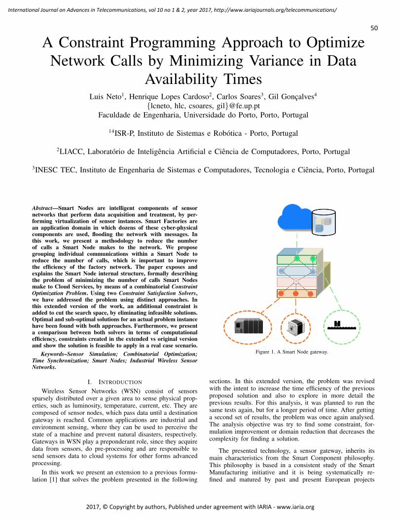
A Constraint Programming Approach to OptimizeNetwork Calls by Minimizing Variance in Data

Availability TimesLuis Neto1, Henrique Lopes Cardoso2, Carlos Soares3, Gil Goncalves4

{lcneto, hlc, csoares, gil}@fe.up.ptFaculdade de Engenharia, Universidade do Porto, Porto, Portugal

14ISR-P, Instituto de Sistemas e Robotica - Porto, Portugal

2LIACC, Laboratorio de Inteligencia Artificial e Ciencia de Computadores, Porto, Portugal

3INESC TEC, Instituto de Engenharia de Sistemas e Computadores, Tecnologia e Ciencia, Porto, Portugal

Abstract—Smart Nodes are intelligent components of sensornetworks that perform data acquisition and treatment, by per-forming virtualization of sensor instances. Smart Factories arean application domain in which dozens of these cyber-physicalcomponents are used, flooding the network with messages. Inthis work, we present a methodology to reduce the numberof calls a Smart Node makes to the network. We proposegrouping individual communications within a Smart Node toreduce the number of calls, which is important to improvethe efficiency of the factory network. The paper exposes andexplains the Smart Node internal structure, formally describingthe problem of minimizing the number of calls Smart Nodesmake to Cloud Services, by means of a combinatorial ConstraintOptimization Problem. Using two Constraint Satisfaction Solvers,we have addressed the problem using distinct approaches. Inthis extended version of the work, an additional constraint isadded to cut the search space, by eliminating infeasible solutions.Optimal and sub-optimal solutions for an actual problem instancehave been found with both approaches. Furthermore, we presenta comparison between both solvers in terms of computationalefficiency, constraints created in the extended vs original versionand show the solution is feasible to apply in a real case scenario.

Keywords–Sensor Simulation; Combinatorial Optimization;Time Synchronization; Smart Nodes; Industrial Wireless SensorNetworks.

I. INTRODUCTION

Wireless Sensor Networks (WSN) consist of sensorssparsely distributed over a given area to sense physical prop-erties, such as luminosity, temperature, current, etc. They arecomposed of sensor nodes, which pass data until a destinationgateway is reached. Common applications are industrial andenvironment sensing, where they can be used to perceive thestate of a machine and prevent natural disasters, respectively.Gateways in WSN play a preponderant role, since they acquiredata from sensors, do pre-processing and are responsible tosend sensors data to cloud systems for other forms advancedprocessing.

In this work we present an extension to a previous formu-lation [1] that solves the problem presented in the following

Figure 1. A Smart Node gateway.

sections. In this extended version, the problem was revisedwith the intent to increase the time efficiency of the previousproposed solution and also to explore in more detail theprevious results. For this analysis, it was planned to run thesame tests again, but for a longer period of time. After gettinga second set of results, the problem was once again analysed.The analysis objective was try to find some constraint, for-mulation improvement or domain reduction that decreases thecomplexity for finding a solution.

The presented technology, a sensor gateway, inherits itsmain characteristics from the Smart Component philosophy.This philosophy is based in a consistent study of the SmartManufacturing initiative and it is being systematically re-fined and matured by past and present European projects

50



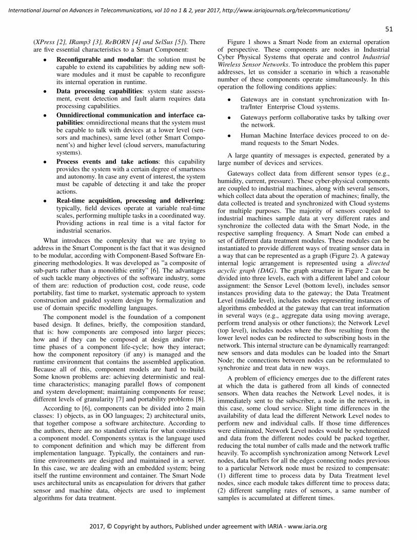
(XPress [2], IRamp3 [3], ReBORN [4] and SelSus [5]). Thereare five essential characteristics to a Smart Component:• Reconfigurable and modular: the solution must be

capable to extend its capabilities by adding new soft-ware modules and it must be capable to reconfigureits internal operation in runtime.

• Data processing capabilities: system state assess-ment, event detection and fault alarm requires dataprocessing capabilities.

• Omnidirectional communication and interface ca-pabilities: omnidirectional means that the system mustbe capable to talk with devices at a lower level (sen-sors and machines), same level (other Smart Compo-nent’s) and higher level (cloud servers, manufacturingsystems).

• Process events and take actions: this capabilityprovides the system with a certain degree of smartnessand autonomy. In case any event of interest, the systemmust be capable of detecting it and take the properactions.

• Real-time acquisition, processing and delivering:typically, field devices operate at variable real-timescales, performing multiple tasks in a coordinated way.Providing actions in real time is a vital factor forindustrial scenarios.

What introduces the complexity that we are trying toaddress in the Smart Component is the fact that it was designedto be modular, according with Component-Based Software En-gineering methodologies. It was developed as ”a composite ofsub-parts rather than a monolithic entity” [6]. The advantagesof such tackle many objectives of the software industry, someof them are: reduction of production cost, code reuse, codeportability, fast time to market, systematic approach to systemconstruction and guided system design by formalization anduse of domain specific modelling languages.

The component model is the foundation of a componentbased design. It defines, briefly, the composition standard,that is: how components are composed into larger pieces;how and if they can be composed at design and/or run-time phases of a component life-cycle; how they interact;how the component repository (if any) is managed and theruntime environment that contains the assembled application.Because all of this, component models are hard to build.Some known problems are: achieving deterministic and real-time characteristics; managing parallel flows of componentand system development; maintaining components for reuse;different levels of granularity [7] and portability problems [8].

According to [6], components can be divided into 2 mainclasses: 1) objects, as in OO languages; 2) architectural units,that together compose a software architecture. According tothe authors, there are no standard criteria for what constitutesa component model. Components syntax is the language usedto component definition and which may be different fromimplementation language. Typically, the containers and run-time environments are designed and maintained in a server.In this case, we are dealing with an embedded system; beingitself the runtime environment and container. The Smart Nodeuses architectural units as encapsulation for drivers that gathersensor and machine data, objects are used to implementalgorithms for data treatment.

Figure 1 shows a Smart Node from an external operationof perspective. These components are nodes in IndustrialCyber Physical Systems that operate and control IndustrialWireless Sensor Networks. To introduce the problem this paperaddresses, let us consider a scenario in which a reasonablenumber of these components operate simultaneously. In thisoperation the following conditions applies:

• Gateways are in constant synchronization with In-tra/Inter Enterprise Cloud systems.

• Gateways perform collaborative tasks by talking overthe network.

• Human Machine Interface devices proceed to on de-mand requests to the Smart Nodes.

A large quantity of messages is expected, generated by alarge number of devices and services.

Gateways collect data from different sensor types (e.g.,humidity, current, pressure). These cyber-physical componentsare coupled to industrial machines, along with several sensors,which collect data about the operation of machines; finally, thedata collected is treated and synchronized with Cloud systemsfor multiple purposes. The majority of sensors coupled toindustrial machines sample data at very different rates andsynchronize the collected data with the Smart Node, in therespective sampling frequency. A Smart Node can embed aset of different data treatment modules. These modules can beinstantiated to provide different ways of treating sensor data ina way that can be represented as a graph (Figure 2). A gatewayinternal logic arrangement is represented using a directedacyclic graph (DAG). The graph structure in Figure 2 can bedivided into three levels, each with a different label and colourassignment: the Sensor Level (bottom level), includes sensorinstances providing data to the gateway; the Data TreatmentLevel (middle level), includes nodes representing instances ofalgorithms embedded at the gateway that can treat informationin several ways (e.g., aggregate data using moving average,perform trend analysis or other functions); the Network Level(top level), includes nodes where the flow resulting from thelower level nodes can be redirected to subscribing hosts in thenetwork. This internal structure can be dynamically rearranged:new sensors and data modules can be loaded into the SmartNode; the connections between nodes can be reformulated tosynchronize and treat data in new ways.

A problem of efficiency emerges due to the different ratesat which the data is gathered from all kinds of connectedsensors. When data reaches the Network Level nodes, it isimmediately sent to the subscriber, a node in the network, inthis case, some cloud service. Slight time differences in theavailability of data lead the different Network Level nodes toperform new and individual calls. If those time differenceswere eliminated, Network Level nodes would be synchronizedand data from the different nodes could be packed together,reducing the total number of calls made and the network trafficheavily. To accomplish synchronization among Network Levelnodes, data buffers for all the edges connecting nodes previousto a particular Network node must be resized to compensate:(1) different time to process data by Data Treatment levelnodes, since each module takes different time to process data;(2) different sampling rates of sensors, a same number ofsamples is accumulated at different times.

51



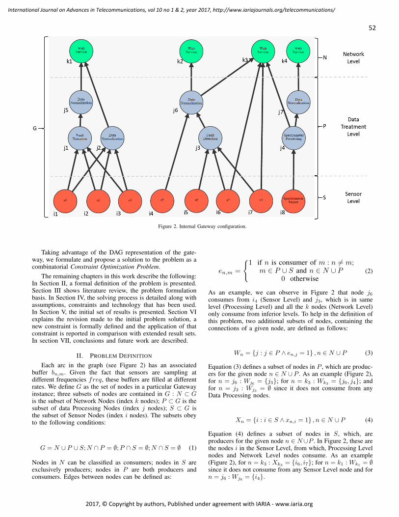
Figure 2. Internal Gateway configuration.

Taking advantage of the DAG representation of the gate-way, we formulate and propose a solution to the problem as acombinatorial Constraint Optimization Problem.

The remaining chapters in this work describe the following:In Section II, a formal definition of the problem is presented.Section III shows literature review, the problem formulationbasis. In Section IV, the solving process is detailed along withassumptions, constraints and technology that has been used.In Section V, the initial set of results is presented. Section VIexplains the revision made to the initial problem solution, anew constraint is formally defined and the application of thatconstraint is reported in comparison with extended result sets.In section VII, conclusions and future work are described.

II. PROBLEM DEFINITION

Each arc in the graph (see Figure 2) has an associatedbuffer bn,m. Given the fact that sensors are sampling atdifferent frequencies freq, these buffers are filled at differentrates. We define G as the set of nodes in a particular Gatewayinstance; three subsets of nodes are contained in G : N ⊂ Gis the subset of Network Nodes (index k nodes); P ⊂ G is thesubset of data Processing Nodes (index j nodes); S ⊂ G isthe subset of Sensor Nodes (index i nodes). The subsets obeyto the following conditions:

G = N ∪ P ∪ S;N ∩ P = ∅;P ∩ S = ∅;N ∩ S = ∅ (1)

Nodes in N can be classified as consumers; nodes in S areexclusively producers; nodes in P are both producers andconsumers. Edges between nodes can be defined as:

en,m =

{1 if n is consumer of m : n 6= m;

m ∈ P ∪ S and n ∈ N ∪ P0 otherwise

(2)

As an example, we can observe in Figure 2 that node j6consumes from i4 (Sensor Level) and j3, which is in samelevel (Processing Level) and all the k nodes (Network Level)only consume from inferior levels. To help in the definition ofthis problem, two additional subsets of nodes, containing theconnections of a given node, are defined as follows:

Wn = {j : j ∈ P ∧ en,j = 1} , n ∈ N ∪ P (3)

Equation (3) defines a subset of nodes in P , which are produc-ers for the given node n ∈ N ∪ P . As an example (Figure 2),for n = j6 : Wj6 = {j3}; for n = k3 : Wk3

= {j6, j4}; andfor n = j3 : Wj3 = ∅ since it does not consume from anyData Processing nodes.

Xn = {i : i ∈ S ∧ xn,i = 1} , n ∈ N ∪ P (4)

Equation (4) defines a subset of nodes in S, which, areproducers for the given node n ∈ N∪P . In Figure 2, these arethe nodes i in the Sensor Level, from which, Processing Levelnodes and Network Level nodes consume. As an example(Figure 2), for n = k3 : Xk3

= {i6, i7}; for n = k1 : Wk1= ∅

since it does not consume from any Sensor Level node and forn = j6 : Wj6 = {i4}.

52



A processing node in P applies an algorithm to transform thedata coming from its associated producers. The data generatedat the sensor level is delivered to the processing nodes as abatch, which contains the number of samples equal to the sizeof the buffer for the corresponding edge.

In order to the processing to be possible, the number ofelements in each collection must be the same. This constraintmust be applied to the subsets Wn and Xn of a given node nin N ∪P , respectively; for that constraint to be respected, thesize of every buffer associated to each element in Wn ∪ Xn

must be the same. Formally this constraint can be representedas:

∀n ∈ N ∪ P,∀m ∈Wn ∪Xn : |bn,m| = f(n) (5)

Where |bn,m| represents the size of the given buffer for thegiven edge en,m and f(n) is the size of any buffer from whichnode n consumes.

The size of a buffer is adjustable and can vary from 1 to1000. The objective of this problem is to arrange a combinationof values to parametrize the size of every buffer |b|, for everyarc in the graph, which minimizes the differences betweentimes at the Network Nodes in which data is available to besent to the network. To calculate the time that takes data to beavailable at every node k ∈ N , the times for all its providersin the graph must be calculated. As data comes in collections(sets of single values), let us define burst as the exact time atwhich data is sent from one provider node to a consumer nodeand represent the burst of a node n as Bn.

The burst of a Sensor Node i is defined by the product ofits sampling frequency and the size of the buffer associatedto the edge en,i we are assuming. That way, every time asample from a sensor is collected, that sample is sent to allconsumers of that sensor. A burst of a Sensor Node to anadjacent consumer node, m, occurs when the buffer for theedge ei,m is completely filled, and is formally represented bythe expression:

Bi,m = freq(i)×|bi,m|×ei,m = 1;∀i ∈ S∧m ∈ P ∪N (6)

For a Data Processing Node, the burst time must contemplateall the burst times from its providers, the time that takes for theassociated function T (f(n)) to treat one data sample and thesize of the buffer associated to the edge en,m we are assuming.The expression which determines the burst time for a DataProcessing Node j to a consumer node m is defined as:

Bj,m = (maxi∈Wj∪Xj(Bi,j) + T (fj)× (|Wj |+ |Xj |))× |bj,m|; ej,m = 1 (7)

We assume that the growth in time complexity of the functionT (fn) : n ∈ P is linear with the number of samples to process.Since the size of each producer buffer is equal, we multiplythe total number of producers of j by the cost of treating asingle sample. To calculate the burst for j1 (see Figure 2), wetake the max burst of Xj1 and sum the product of T (fj1) (timeto process one sensor sample) with the number of elements inXj1 (which corresponds to the producers i1, i2 and i3).

Finally, to calculate the burst of a Network Node k ∈ N :

Bk = maxi∈Xk∪Wk

(Bi,k) (8)

Using the expression to calculate the burst for each NetworkNode, the objective is to minimize the variance of burst for allthe Network Nodes and also minimize the sum of all buffersizes in the DAG. By varying the size of the buffers in thegraph, the variance of all burst times for Network Nodes andthe sum of all buffer sizes are minimized. With a varianceof zero or closer, data from different Network Nodes can bepacked in the same payload and sent to the subscribers in thenetwork. Even if the quantity of data exceeds the maximumpayload size for the protocol in use, or the physical link beingused, the number of connections needed is far less than itis when using the original strategy of independent calls. Thenumber of buffers |P ∪N |, times an upper bound buffer sizeof 1000 is multiplied by the variance. This way, the variancehas more impact in the search of an optimal solution than thesum of all buffer sizes.

V (Bk)× 1000× |P ∪N |+∑

n∈|P∪N |

∑m∈Wn∪Xn

|bn,m| (9)

As follows from Equation (9), minimizing variance of bursttimes for network nodes is the major concern. To reflect this,the variance is multiplied by the maximum possible size for abuffer (1000, which is a reasonable number of samples for asensor), times the number of Processing and Network nodes.This will drive the solver to focus on a solution with lessvariance, and break ties by considering the minimal buffer sizes(as these incur a cost). With a variance of 0 at the NetworkLevel nodes, all data produced can be sent to the cloud usingthe same call. If variance is higher than 0, a threshold must beused to decide the maximum reasonable time to wait betweenbursts. In comparison with individual calls strategy – a callmade every time a burst at the Network Level occurs – thenumber of calls to the cloud is minimized as a consequence.The theoretical search space of the problem is En, where Erepresents the total number of edges in the graph and n = 1000is the Buffer Size domain upper bound. The real search space,imposed by the constraint of Equation (5), can be determinedby Fn, where F = |P |+ |N | is the total number of Processingand Network nodes in the graph.

III. RELATED WORK

To the best of our knowledge, there is no scientific literatureor works that cover this exact problem. The problem presentedin this work emerged due to the very specific nature of SmartNodes applied to industrial monitoring situations. Since anexact formulation or solution to this problem could not befound, the related works presented are analogous in the sensethat some knowledge could be used to refine the modellingand solutions presented.

The theoretical background behind this problem has a largespectrum of application. The problem of modelling buffersizes is mostly applied to network routing, to which theworks [9],[10] and [11] are examples. As we are not interestedin dealing with networks intrinsic characteristics, those buffer

53



optimization problems can hardly be extrapolated to this work.The domain of Wireless Sensor Networks (WSN) is anotherscope of application of buffer modelling optimization, withrelevant literature in this domain; the section of Routingproblems in [12] covers a great number of important works re-garding Flow Based Optimization Models, for data aggregationand routing problems. WSN optimization models care withconstraints that this problem modulation does not cover, suchas: residual energy of nodes, link properties, network lifetime,network organization and routing strategies.

A relevant work in WSN revealed to be of the major inter-est for this work. The authors presented and solved the problemof removing inconsistent time offsets, in time synchronizationprotocols for WSN [13]. The problem presented has a highdegree of similarity with the case we are dealing. The problemis represented by a Time Difference Graph (TDG), where eachnode is a sensor, every sensor has local time and every arc hasan associated cost time given by a function. The solution to theproblem is given by a Constraint Satisfaction Problem (CSP)approach. For every arc in the graph there exists an adjustmentvariable (analogous to the buffer size in this case), assignmentsare made to the variables to find the largest consistent sub-graph, i.e., a sub-graph in which inconsistent time offsets areeliminated.

Focusing the search in the literature domain of CSP prob-lems, several works were revealed in the sub-domain of bal-ancing, planning and scheduling activities that can be relatedto this application [14][15][16][17][18]. Namely, models ofcombinatorial optimization for minimizing the maximum/totallateness/tardiness of directed graphs of tasks with precedenceand time constraints [14][18]. These problems are analogousto this work, and due to a simplified formulation with thesame constraints (precedences and time between nodes), canbe easily extrapolated to our case.

IV. IMPLEMENTING AND TESTING

A. Problem AssumptionsThe Smart Node application has several interfaces for real

sensors, the physical connections range from radio frequencyto cabled protocols. By testing this model with simulatedscenarios, we assume no interference or noise of any type cancause disturbance in the sampling frequency. In a real casescenario, a sensor could enter in an idle state for a varietyof reasons. In that case, data would not be transmitted at all,causing the transmission of data to the Cloud to be postponedfor undefined time, waiting for the Network Level node burstdepending on the idle sensor. For simplification, we assumea sensor never enters an idle state. Also, it is assumed thatthe time that takes to treat one sample of data will increaselinearly for more than one sample, as mentioned for T (fj)when introducing Equation (7).

B. Constraint Satisfaction Problem SolversFor comparison of performance purposes we implemented

the problem using both OptaPlanner and SICStus Prolog. Asthe Smart Node is implemented in Java we can take advantageof a direct integration with OptaPlanner in future. On theother hand, we expected that SICStus Prolog would producethe same results with better computation times because of thelightweight implementation and optimized constraint library.Using these premises and the results presented in the next

section a grounded decision about what solver to use in futureimplementations of the Smart Node can be made.

C. TestsTo validate the problem solutions, several DAG configura-

tions were tested using the two implemented versions, based onOptaPlanner and SICStus Prolog, as described in Section IV.To test the implementations an algorithm to generate instancesof the problem was built. The script generates instances of theSmart Node internal structure, DAG’s, with a given number ofProcessing and Network nodes. Algorithm 1 briefly illustratesthe approach:

Data: G← S ∪ P ∪NResult: Smart Node internal configuration GnotV isitedNodes← G;Pnodes← randomInteger( |P∪N |

2 , |P ∪N | − 2);Nnodes← nNodes− Pnodes;Snodes←randomInteger(nNodes

2 , nNodes + nNodes2 );

G← S, P,N ←generateNodes(Snodes, Pnodes,Nnodes);remainingEdges← Pnodes× 2 +Nnodes+Snodes;while remainingEdges > 0 do

if node← notV isitedNodes.nextNode() thennotV isitedNodes.remove(node);

elsenode← G.randomNode();

endif node is S then

connect to a random P or S node, disconnectednodes first;remainingEdges−−;

else if node is P thenget connection from a random P or S node,disconnected nodes first;

connect to a random P or S node, disconnectednodes first;remainingEdges−−;remainingEdges−−;

elseget connection from random a P or S node,disconnected nodes first;remainingEdges−−;

endend

Algorithm 1: Smart Node instance generation.

Real scenarios generally have a higher number of SensorNodes, followed by a small number of Processing Nodes andan even smaller number of Network Nodes. Typically, the totalnumber of nodes does not exceed 30 per operation. The in-stance generator picks aleatory numbers for the nodes boundedby a real case scenario application. Sampling frequencies forthe sensors are assumed to vary from 400 to 2000 milliseconds.Functions to treat data in Processing Nodes are not typicallycomplex. We measured the real case scenario functions to treatthe minimum amount of data (1 sample) and we got valuesranging from 0.19 to 0.38 milliseconds. To cover the buffersize domain, we need to take the worst case, 1000 samples.Given best and worst cases, the values attributed to cost of

54



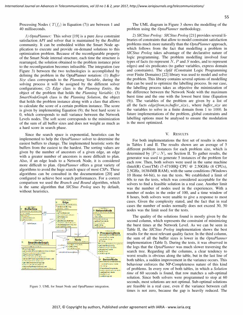
Processing Nodes ( T (fj) in Equation (7)) are between 1 and40 milliseconds.

1) OptaPlanner: This solver [19] is a pure Java constraintsatisfaction API and solver that is maintained by the RedHatcommunity. It can be embedded within the Smart Node ap-plication to execute and provide on-demand solutions to thisoptimization problem. Because of the reconfigurable propertyof the Smart Node internal structure, each time the structure isrearranged, the solution obtained to the problem instance priorto the reconfiguration becomes infeasible. The integration (seeFigure 3) between the two technologies is accomplished bydefining the problem in the OptaPlanner notation: (1) BufferSize class corresponds to the Planning Variable, during thesolving process it will be assigned by the different solverconfigurations; (2) Edge class is the Planning Entity, theobject of the problem that holds the Planning Variable; (3)SmartNodeGraph class is the Planning Solution, the objectthat holds the problem instance along with a class that allowsto calculate the score of a certain problem instance. The scoreis given by implementing Equation (9); the best hard score is0, which corresponds to null variance between the NetworkLevels nodes. The soft score corresponds to the minimizationof the sum of all buffer sizes and does not weight as much asa hard score in search phase.

Since the search space is exponential, heuristics can beimplemented to help the OptaPlanner solver to determine theeasiest buffers to change. The implemented heuristic sorts thebuffers from the easiest to the hardest. The sorting values aregiven by the number of ancestors of a given edge, an edgewith a greater number of ancestors is more difficult to plan.Also, if an edge leads to a Network Node, it is consideredmore difficult to plan. OptaPlanner offers a great variety ofalgorithms to avoid the huge search space of most CSPs. Thesealgorithms can be consulted in the documentation [20] andconfigured to achieve best search performances. For a correctcomparison we used the Branch and Bound algorithm, whichis the same algorithm that SICStus Prolog uses by default,without heuristics.

Figure 3. UML for Smart Node and OptaPlanner integration.

The UML diagram in Figure 3 shows the modelling of theproblem using the OptaPlanner methodology.

2) SICStus Prolog: SICStus Prolog [21] provides several li-braries of constraints that allow to model constraint satisfactionproblems much more naturally than the OptaPlanner approach,which follows from the fact that modelling a problem inSICStus Prolog takes advantage of the declarative nature oflogic programming. The problem modelling involved fourtypes of facts (to represent N , P and S nodes, and to representedges) and six predicates (to gather variables, express domainand constraints). The clpfd (Constraint Logic Programmingover Finite Domains) [22] library was used to model and solvethe problem. This library contains several options of modellingthat can be used to optimize the labelling process. In our case,the labelling process takes as objective the minimization ofthe difference between the Network Node with the maximumburst time and the one with the lowest burst time (Equation(9)). The variables of the problem are given by a list ofall the facts edge(from,to,buffer size)., where buffer size arethe variables to solve in a finite domain from 1 to 1000. Infuture implementations of the problem, global constraints andlabelling options must be analysed to ensure the modulationis the most optimized.

V. RESULTS

For both implementations the first set of results is shownin Tables I and II. The results shown are an average of 5different problem instances for each problem size, which isdetermined by |P ∪N |, see Section II. To gather results, thegenerator was used to generate 5 instances of the problem foreach row. Then, both solvers were used in the same machine(Intel(R) Core(TM) i7-4710HQ CPU @ 2.50GHz (8 CPUs),2.5GHz, 16384MB RAM), with the same conditions (Windows10 Home 64-bit), to run the tests. We established a limit of60s to run the tests, which was considered acceptable for thesolvers to find a feasible solution in a real case. Another limitwas the number of nodes used in the experiences. With anumber of nodes in the order of 100, and a time window of8 hours, both solvers were unable to give a response to mostcases. Given the complexity stated, and the fact that in realcases the number of nodes normally does not exceed 30, 50nodes was the limit used for the tests.

The quality of the solutions found is mostly given by thesecond column, which represents the constraint of minimizingthe burst times at the Network Level. As we can be seen inTable II, the SICStus Prolog implementation shows the bestresults for the most relevant quality factor. In the third column,the sum of all the buffer sizes is lower in the OptaPlannerimplementation (Table I). During the tests, it was observed inthe logs that the OptaPlanner was much slower traversing thesearch tree. Regarding all the columns, a clear tendency toworst results is obvious along the table, but in the last line ofboth tables, a sudden improvement in the variance occurs. Thisbehaviour enforces the NP-Completeness nature of this kindof problems. In every row of both tables, in which a Solutiontime of 60 seconds is found, that row matches a sub-optimalsolution. Since both solvers were programmed to stop at 60seconds, most solutions are not optimal. Sub-optimal solutionsare feasible in a real case, even if the variance between calltimes is not zero, because the gap is heavily reduced. The

55



TABLE I. OptaPlanner results

TABLE II. SICStus results

Smart Component can define a time window with the size ofthe variance, and this way, include all results in the same call.

VI. PROBLEM REVISION

In this section, the second set of results is presented anddiscussed. A deeper problem analysis was conducted and theconclusions of this analysis are applied in a third set of tests.

Firstly, the time limit imposed to the search conducted inthe previous results (Table I and Table II), was extended to 9hours. To add more detail to the study, two new columns wereadded to the new results (Table III, Table IV and Table V). Theinitial variance ∆Vi(Bk), introduced in the first column, is thevariance calculated with all buffer sizes set to the minimumsize of 1. This column was introduced to give an idea of byhow much is the time difference between the optimized versionis produced and the first approach - set all buffers to samevalue, 1. The second column introduced was ”Total Searchtime (s)”, it indicates the total amount of time that the searchprocess took. For 32400 seconds (or 9 hours), it indicates anon optimal solution, because the search phase surpassed thetime limit established. When the time indicated is the same as

in ”Total Search time (s)”, it means that an optimal solutionwas found timely. ”Total Search time (s)” indicates the timethat took to find the solution presented in the table, which isthe last optimization found before the time limit was exceeded.With this separation it is possible to see that most of the results(∆Vf (Bk)) are found in a average time of 2.46 hours for theSICStus implementation. These results motivated a problemrevision to decrease the search time and that is addressed inthe following sections.

TABLE III. OptaPlanner Extended Results

TABLE IV. SICStus Extended Results

A. Proposed EnhancementTo analyse the problem more deeply, let us consider the

buffers in the graph were adjusting its size is really critical.The buffers in inferior levels, all that connect P and S nodes,

56



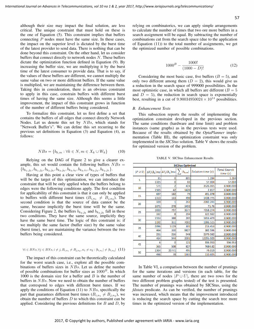
although their size may impact the final solution, are lesscritical. The unique constraint that must hold on these isthe one of Equation (5). This constraint implies that buffersconnecting P nodes must have the same size. In these cases,the impact on the superior level is dictated by the burst timeof the latest provider to send data. There is nothing that can bedone beyond this constraint. On the other hand, let us considerbuffers that connect directly to network nodes N . These buffersdictate the optimization function defined in Equation (9). Byincreasing the buffer size, we are multiplying it by the bursttime of the latest consumer to provide data. That is to say, ifthe values of these buffers are different, we cannot multiply thesame value on two or more different buffers. If the same valueis multiplied, we are maintaining the difference between them.Taking this in consideration, there is an obvious constraintto apply in this case, constrain buffers with different bursttimes of having the same size. Although this seems a littleimprovement, the impact of this constraint grows in functionof the number of different buffers being considered.

To formalize this constraint, let us first define a set thatcontains the buffers of all edges that connect directly NetworkNodes. Let us denote this set by NBs, which stands for”Network Buffer’s”. We can define this set recurring to theprevious set definitions in Equation (3) and Equation (4), asfollows:

NBs = {bk,m : ∀k ∈ N,m ∈ Xk ∪Wk} (10)

Relying on the DAG of Figure 2 to give a clearer ex-ample, this set would contain the following buffers NBs ={bk1,j5 , bk1,j2 , bk2,j6 , bk3,j6 , bk3,i6 , bk3,i7 , bk3,j4 , bk4,j7}.

Having at this point a clear view of types of buffers thatwill be the target of this optimization, we can introduce theconstraint that will be only applied when the buffers belong toedges were the following conditions apply. The first conditionfor applicability of this constraint is that it can only be appliedto buffers with different burst times (Bi,n1

6= Bj,n2). The

second condition is that the source of data cannot be thesame, because implicitly the burst time will be the same.Considering Figure 2, the buffers bk2,j6 and bk3,j6 fall in thesetwo conditions. They have the same source, implicitly theyhave the same burst time. The logic of this constraint is: ifwe multiply the same factor (buffer size) by the same value(burst time), we are maintaining the variance between the twobuffers being considered.

∀i ∈ BNs, ∀j ∈ BNs, i 6= j, Bi,n16= Bj,n2

, n1 6= n2 : |bi,n1| 6= |bi,n2

| (11)

The impact of this constraint can be theoretically calculatedfor the worst search case, i.e., explore all the possible com-binations of buffers sizes in NBs. Let us define the numberof possible combinations for buffer sizes as 1000B . In which1000 is the domain size for a buffer and B is the number ofbuffers in NBs. Now we need to obtain the number of buffersthat correspond to edges with different burst times. If weapply the conditions of Equation (11) to NBs, specifically thepart that guarantees different burst times (Bi,n1

6= Bj,n2), we

obtain the number of buffers D to which this constraint can beapplied. Considering the previous definitions for B and D, by

relying on combinatorics, we can apply simple arrangementsto calculate the number of times that two ore more buffers in asearch assignment will be equal. By subtracting the number ofcombinations cut from the search space (due to the applicationof Equation (11)) to the total number of assignments, we getthe optimized number of possible combinations.

1000B − 1000!

(1000−D)!(12)

Considering the most basic case, five buffers (B = 5), andonly two different among them (D = 2), this would give usa reduction in the search space of 999000 possibilities. In themost optimistic case, in which all buffers are different (B = 5and D = 5), the reduction in search space is exponentiallybest, resulting in a cut of 9.90034950024× 1014 possibilities.

B. Enhancement TestsThis subsection reports the results of implementing the

optimization constraint developed in the previous section.The same conditions (hardware and time limit) and probleminstances (same graphs) as in the previous tests were used.Because of the results obtained by the OptaPlanner imple-mentation (Table III), the optimization constraint was onlyimplemented in the SICStus solution. Table V shows the resultsfor optimized version of the problem.

TABLE V. SICStus Enhancement Results

In Table VI, a comparison between the number of pruningsfor the same iterations and versions (in each table, for thesame number of nodes |P ∪ U |, there are two rows for thetwo different problem graphs tested) of the test is presented.The number of prunings was obtained by SICStus, using thefdstats predicate. As can be verified, the number of pruningswas increased, which means that the improvement introducedis reducing the search space by cutting the search tree moretimes in the optimized version of the implementation.

57



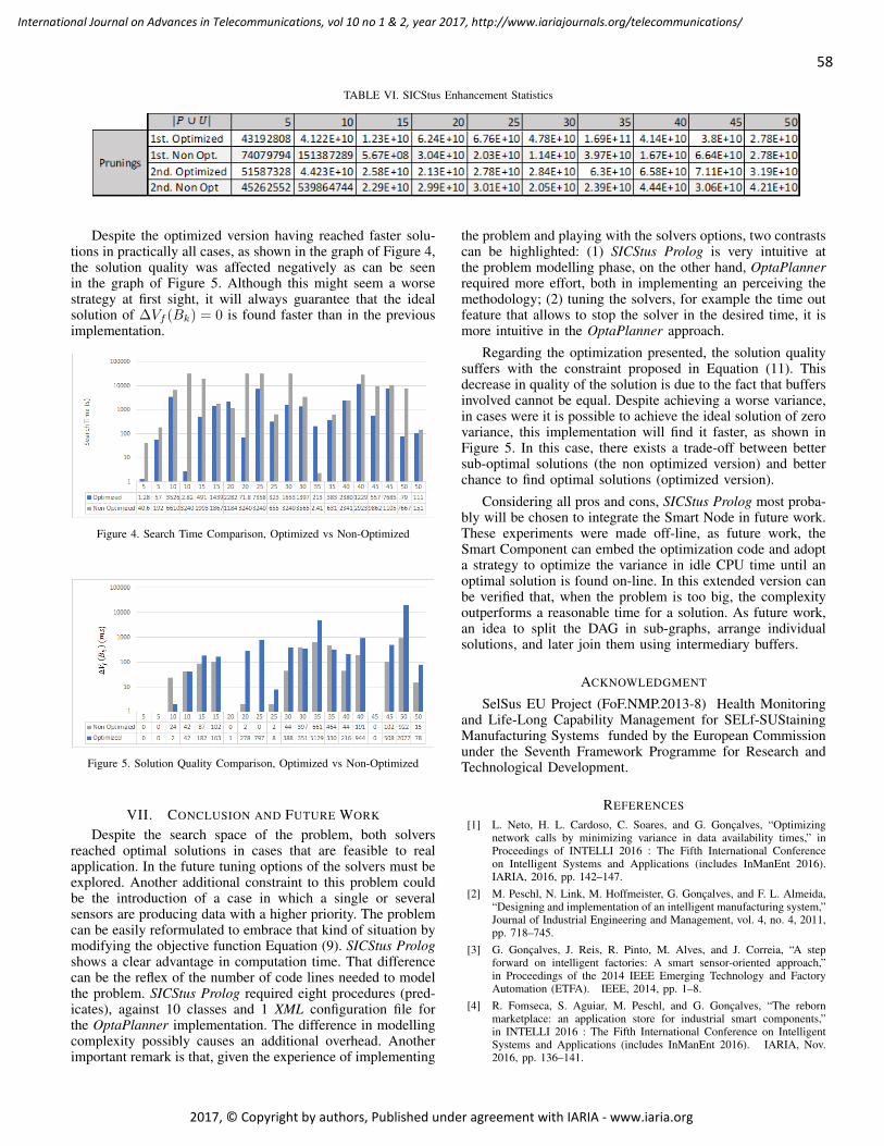
TABLE VI. SICStus Enhancement Statistics

Despite the optimized version having reached faster solu-tions in practically all cases, as shown in the graph of Figure 4,the solution quality was affected negatively as can be seenin the graph of Figure 5. Although this might seem a worsestrategy at first sight, it will always guarantee that the idealsolution of ∆Vf (Bk) = 0 is found faster than in the previousimplementation.

Figure 4. Search Time Comparison, Optimized vs Non-Optimized

Figure 5. Solution Quality Comparison, Optimized vs Non-Optimized

VII. CONCLUSION AND FUTURE WORK

Despite the search space of the problem, both solversreached optimal solutions in cases that are feasible to realapplication. In the future tuning options of the solvers must beexplored. Another additional constraint to this problem couldbe the introduction of a case in which a single or severalsensors are producing data with a higher priority. The problemcan be easily reformulated to embrace that kind of situation bymodifying the objective function Equation (9). SICStus Prologshows a clear advantage in computation time. That differencecan be the reflex of the number of code lines needed to modelthe problem. SICStus Prolog required eight procedures (pred-icates), against 10 classes and 1 XML configuration file forthe OptaPlanner implementation. The difference in modellingcomplexity possibly causes an additional overhead. Anotherimportant remark is that, given the experience of implementing

the problem and playing with the solvers options, two contrastscan be highlighted: (1) SICStus Prolog is very intuitive atthe problem modelling phase, on the other hand, OptaPlannerrequired more effort, both in implementing an perceiving themethodology; (2) tuning the solvers, for example the time outfeature that allows to stop the solver in the desired time, it ismore intuitive in the OptaPlanner approach.

Regarding the optimization presented, the solution qualitysuffers with the constraint proposed in Equation (11). Thisdecrease in quality of the solution is due to the fact that buffersinvolved cannot be equal. Despite achieving a worse variance,in cases were it is possible to achieve the ideal solution of zerovariance, this implementation will find it faster, as shown inFigure 5. In this case, there exists a trade-off between bettersub-optimal solutions (the non optimized version) and betterchance to find optimal solutions (optimized version).

Considering all pros and cons, SICStus Prolog most proba-bly will be chosen to integrate the Smart Node in future work.These experiments were made off-line, as future work, theSmart Component can embed the optimization code and adopta strategy to optimize the variance in idle CPU time until anoptimal solution is found on-line. In this extended version canbe verified that, when the problem is too big, the complexityoutperforms a reasonable time for a solution. As future work,an idea to split the DAG in sub-graphs, arrange individualsolutions, and later join them using intermediary buffers.

ACKNOWLEDGMENT

SelSus EU Project (FoF.NMP.2013-8) Health Monitoringand Life-Long Capability Management for SELf-SUStainingManufacturing Systems funded by the European Commissionunder the Seventh Framework Programme for Research andTechnological Development.

REFERENCES

[1] L. Neto, H. L. Cardoso, C. Soares, and G. Goncalves, “Optimizingnetwork calls by minimizing variance in data availability times,” inProceedings of INTELLI 2016 : The Fifth International Conferenceon Intelligent Systems and Applications (includes InManEnt 2016).IARIA, 2016, pp. 142–147.

[2] M. Peschl, N. Link, M. Hoffmeister, G. Goncalves, and F. L. Almeida,“Designing and implementation of an intelligent manufacturing system,”Journal of Industrial Engineering and Management, vol. 4, no. 4, 2011,pp. 718–745.

[3] G. Goncalves, J. Reis, R. Pinto, M. Alves, and J. Correia, “A stepforward on intelligent factories: A smart sensor-oriented approach,”in Proceedings of the 2014 IEEE Emerging Technology and FactoryAutomation (ETFA). IEEE, 2014, pp. 1–8.

[4] R. Fomseca, S. Aguiar, M. Peschl, and G. Goncalves, “The rebornmarketplace: an application store for industrial smart components,”in INTELLI 2016 : The Fifth International Conference on IntelligentSystems and Applications (includes InManEnt 2016). IARIA, Nov.2016, pp. 136–141.

58



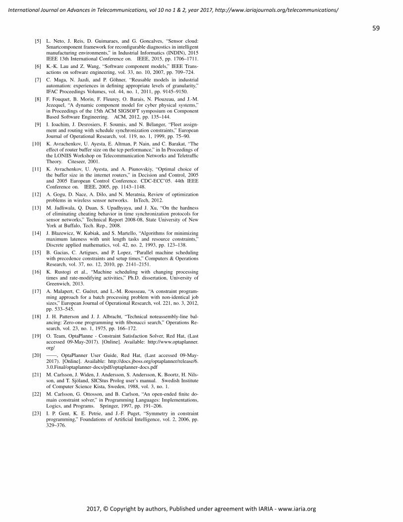
[5] L. Neto, J. Reis, D. Guimaraes, and G. Goncalves, “Sensor cloud:Smartcomponent framework for reconfigurable diagnostics in intelligentmanufacturing environments,” in Industrial Informatics (INDIN), 2015IEEE 13th International Conference on. IEEE, 2015, pp. 1706–1711.

[6] K.-K. Lau and Z. Wang, “Software component models,” IEEE Trans-actions on software engineering, vol. 33, no. 10, 2007, pp. 709–724.

[7] C. Maga, N. Jazdi, and P. Gohner, “Reusable models in industrialautomation: experiences in defining appropriate levels of granularity,”IFAC Proceedings Volumes, vol. 44, no. 1, 2011, pp. 9145–9150.

[8] F. Fouquet, B. Morin, F. Fleurey, O. Barais, N. Plouzeau, and J.-M.Jezequel, “A dynamic component model for cyber physical systems,”in Proceedings of the 15th ACM SIGSOFT symposium on ComponentBased Software Engineering. ACM, 2012, pp. 135–144.

[9] I. Ioachim, J. Desrosiers, F. Soumis, and N. Belanger, “Fleet assign-ment and routing with schedule synchronization constraints,” EuropeanJournal of Operational Research, vol. 119, no. 1, 1999, pp. 75–90.

[10] K. Avrachenkov, U. Ayesta, E. Altman, P. Nain, and C. Barakat, “Theeffect of router buffer size on the tcp performance,” in In Proceedings ofthe LONIIS Workshop on Telecommunication Networks and TeletrafficTheory. Citeseer, 2001.

[11] K. Avrachenkov, U. Ayesta, and A. Piunovskiy, “Optimal choice ofthe buffer size in the internet routers,” in Decision and Control, 2005and 2005 European Control Conference. CDC-ECC’05. 44th IEEEConference on. IEEE, 2005, pp. 1143–1148.

[12] A. Gogu, D. Nace, A. Dilo, and N. Meratnia, Review of optimizationproblems in wireless sensor networks. InTech, 2012.

[13] M. Jadliwala, Q. Duan, S. Upadhyaya, and J. Xu, “On the hardnessof eliminating cheating behavior in time synchronization protocols forsensor networks,” Technical Report 2008-08, State University of NewYork at Buffalo, Tech. Rep., 2008.

[14] J. Błazewicz, W. Kubiak, and S. Martello, “Algorithms for minimizingmaximum lateness with unit length tasks and resource constraints,”Discrete applied mathematics, vol. 42, no. 2, 1993, pp. 123–138.

[15] B. Gacias, C. Artigues, and P. Lopez, “Parallel machine schedulingwith precedence constraints and setup times,” Computers & OperationsResearch, vol. 37, no. 12, 2010, pp. 2141–2151.

[16] K. Rustogi et al., “Machine scheduling with changing processingtimes and rate-modifying activities,” Ph.D. dissertation, University ofGreenwich, 2013.

[17] A. Malapert, C. Gueret, and L.-M. Rousseau, “A constraint program-ming approach for a batch processing problem with non-identical jobsizes,” European Journal of Operational Research, vol. 221, no. 3, 2012,pp. 533–545.

[18] J. H. Patterson and J. J. Albracht, “Technical noteassembly-line bal-ancing: Zero-one programming with fibonacci search,” Operations Re-search, vol. 23, no. 1, 1975, pp. 166–172.

[19] O. Team, OptaPlanne - Constraint Satisfaction Solver, Red Hat, (Lastaccessed 09-May-2017). [Online]. Available: http://www.optaplanner.org/

[20] ——, OptaPlanner User Guide, Red Hat, (Last accessed 09-May-2017). [Online]. Available: http://docs.jboss.org/optaplanner/release/6.3.0.Final/optaplanner-docs/pdf/optaplanner-docs.pdf

[21] M. Carlsson, J. Widen, J. Andersson, S. Andersson, K. Boortz, H. Nils-son, and T. Sjoland, SICStus Prolog user’s manual. Swedish Instituteof Computer Science Kista, Sweden, 1988, vol. 3, no. 1.

[22] M. Carlsson, G. Ottosson, and B. Carlson, “An open-ended finite do-main constraint solver,” in Programming Languages: Implementations,Logics, and Programs. Springer, 1997, pp. 191–206.

[23] I. P. Gent, K. E. Petrie, and J.-F. Puget, “Symmetry in constraintprogramming,” Foundations of Artificial Intelligence, vol. 2, 2006, pp.329–376.

59



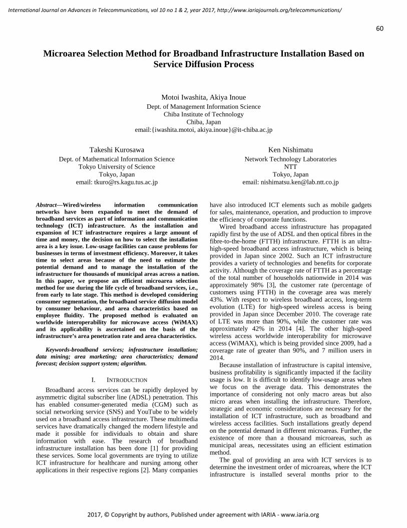
Microarea Selection Method for Broadband Infrastructure Installation Based on Service Diffusion Process

Motoi Iwashita, Akiya Inoue Dept. of Management Information Science

Chiba Institute of Technology Chiba, Japan

email:{iwashita.motoi, akiya.inoue}@it-chiba.ac.jp

Takeshi Kurosawa Dept. of Mathematical Information Science

Tokyo University of Science Tokyo, Japan

email: [email protected]

Ken Nishimatu Network Technology Laboratories

NTT Tokyo, Japan

email: [email protected]

Abstract—Wired/wireless information communication networks have been expanded to meet the demand of broadband services as part of information and communication technology (ICT) infrastructure. As the installation and expansion of ICT infrastructure requires a large amount of time and money, the decision on how to select the installation area is a key issue. Low-usage facilities can cause problems for businesses in terms of investment efficiency. Moreover, it takes time to select areas because of the need to estimate the potential demand and to manage the installation of the infrastructure for thousands of municipal areas across a nation. In this paper, we propose an efficient microarea selection method for use during the life cycle of broadband services, i.e., from early to late stage. This method is developed considering consumer segmentation, the broadband service diffusion model by consumer behaviour, and area characteristics based on employee fluidity. The proposed method is evaluated on worldwide interoperability for microwave access (WiMAX) and its applicability is ascertained on the basis of the infrastructure’s area penetration rate and area characteristics.

Keywords-broadband services; infrastructure installation; data mining; area marketing; area characteristics; demand forecast; decision support system; algorithm.

I. INTRODUCTION Broadband access services can be rapidly deployed by

asymmetric digital subscriber line (ADSL) penetration. This has enabled consumer-generated media (CGM) such as social networking service (SNS) and YouTube to be widely used on a broadband access infrastructure. These multimedia services have dramatically changed the modern lifestyle and made it possible for individuals to obtain and share information with ease. The research of broadband infrastructure installation has been done [1] for providing these services. Some local governments are trying to utilize ICT infrastructure for healthcare and nursing among other applications in their respective regions [2]. Many companies

have also introduced ICT elements such as mobile gadgets for sales, maintenance, operation, and production to improve the efficiency of corporate functions.

Wired broadband access infrastructure has propagated rapidly first by the use of ADSL and then optical fibres in the fibre-to-the-home (FTTH) infrastructure. FTTH is an ultra-high-speed broadband access infrastructure, which is being provided in Japan since 2002. Such an ICT infrastructure provides a variety of technologies and benefits for corporate activity. Although the coverage rate of FTTH as a percentage of the total number of households nationwide in 2014 was approximately 98% [3], the customer rate (percentage of customers using FTTH) in the coverage area was merely 43%. With respect to wireless broadband access, long-term evolution (LTE) for high-speed wireless access is being provided in Japan since December 2010. The coverage rate of LTE was more than 90%, while the customer rate was approximately 42% in 2014 [4]. The other high-speed wireless access worldwide interoperability for microwave access (WiMAX), which is being provided since 2009, had a coverage rate of greater than 90%, and 7 million users in 2014.

Because installation of infrastructure is capital intensive, business profitability is significantly impacted if the facility usage is low. It is difficult to identify low-usage areas when we focus on the average data. This demonstrates the importance of considering not only macro areas but also micro areas when installing the infrastructure. Therefore, strategic and economic considerations are necessary for the installation of ICT infrastructure, such as broadband and wireless access facilities. Such installations greatly depend on the potential demand in different microareas. Further, the existence of more than a thousand microareas, such as municipal areas, necessitates using an efficient estimation method.

The goal of providing an area with ICT services is to determine the investment order of microareas, where the ICT infrastructure is installed several months prior to the

60



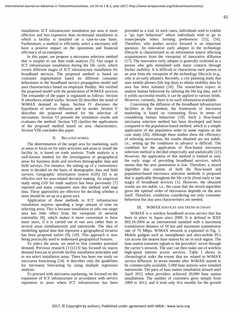
installation. ICT infrastructure installation per area is more effective and less expensive than on-demand installation in which a facility is installed on a case-to-case basis. Furthermore, a method to efficiently select a microarea will have a positive impact on the operations and financial efficiency of an enterprise.

In this paper, we propose a microarea selection method that is simpler to use than trade analysis [5]. Our target is ICT infrastructure installation during the life cycle, which covers different stages of ICT infrastructure installation for broadband services. The proposed method is based on consumer segmentation based on different consumer behaviours in the broadband service propagation model and area characteristics based on employee fluidity. We verified the proposed model with the penetration of WiMAX services. The remainder of the paper is organized as follows: Section II introduces related works. Section III describes the trend of WiMAX demand in Japan. Section IV discusses the hypothesis of service diffusion and its model. Section V describes the proposed method for the selection of microareas. Section VI presents the simulation results and evaluates the method. Section VII clarifies the applications of the proposed method based on area characteristics. Section VIII concludes this paper.

II. RELATED WORKS The determination of the target area for marketing, such

as areas to focus on for sales activities and areas to install the facility in, is based on trade analysis. Trade analysis is a well-known method for the investigation of geographical areas for business deals and involves demographic data and field surveys. For instance, the setting up of a convenience store is decided on the basis of demographic data and field surveys. Geographic information system (GIS) [6] is an effective tool for area-related decision making. An empirical study using GIS for trade analysis has been previously [7] reported and many companies uses this method with map data. These approaches are effective for deciding whether a store should be set up in a given area.

Application of these methods to ICT infrastructure installation requires spending a large amount of time on selecting areas. This is because installation in only one target area has little effect from the viewpoint of network externality [8], which makes it more convenient to have more users, if it is carried out in one area rather than in several areas simultaneously and nationwide. The idea of modelling spatial data that represent a geographical location has been proposed earlier [9], [10]. This approach is now being practically used to understand geographical features.

To select the areas, we need to first consider potential demand. Previous research [11]-[13] has focused on macro demand forecast to provide facility installation principles and to not select installation areas. There has been one study on microarea forecasting [14]. It describes only the guidelines for microarea forecasting by using multiple regression analysis.

To proceed with microarea marketing, we focused on the expansion of ICT infrastructure in accordance with service reputation in areas where ICT infrastructure has been

provided as a trial. In such cases, individuals tend to exhibit a “go type behaviour” where individuals tend to go to issues/people when forming preferences [15], [16]. Therefore, who pushes service forward is an important question. An innovative early adopter in the technology lifecycle is characterized as an information source affecting acquaintances from the viewpoint of innovative diffusion [17]. The innovative early adopter is generally reckoned as a person who gets stimulated with many contacts through his/her mobility. It is difficult to characterise each person in an area from the viewpoint of the technology lifecycle (e.g., who is an early adopter). Recently, a city planning study that uses mobile phones (life log data) to obtain mobility data by area has been initiated [18]. The researchers expect to analyse human behaviour by utilizing the life log data, and if it yields successful results, it can be applied to various fields. However, currently, there is no such information available.

Concerning the diffusion of the broadband infrastructure facilities at the moment, the framework of microarea marketing is based on commuting flows in terms of considering human behaviour [19]. Such a flow-based microarea selection method has been developed and been compared to the population-based method, which is a simple application of the population order in some regions as the case study [20]. Although these studies show the efficiency of selecting microareas, the results obtained are not stable; i.e., setting up the conditions in advance is difficult. The condition for the application of flow-based microarea selection method is decided empirically and analytically [21]. However, the application of this method is limited to only the early stage of providing broadband services, which means that the area penetration is low. Therefore, a mixed algorithm that consists of both the flow-based and population-based microarea selection methods is proposed that is applicable throughout the life cycle (from early to late stage) of broadband services [1]. However, the obtained results are not stable, i.e., the cause that the mixed algorithm gives the optimal order of microareas depends on the area itself. Therefore, conditions considering not only consumer behaviour but also area characteristics are needed.

III. WIMAX SERVICES AND TREND IN JAPAN WiMAX is a wireless broadband access service that has

been in place in Japan since 2009. It is defined in IEEE 802.16-2004 as an international standard with a maximum transmission distance of 50 km and maximum transmission rate of 70 Mbps. WiMAX network is explained in Fig. 1. Mobile gadgets such as smartphones and ultra-mobile PCs can access the nearest base station by air in each region. The base station transmits signals to the providers’ server through the carrier’s network. The user can then make use of wireless high-speed internet access services. Table I shows in chronological order the events that are related to WiMAX service diffusion. In seven months after WiMAX started to be commercially available, 5,000 base stations were installed nationwide. The pace of base station installation slowed until April 2012 when providers achieved 20,000 base station installations. The number of customers grew steeply from 2009 to 2013, and it took only five months for the growth

61



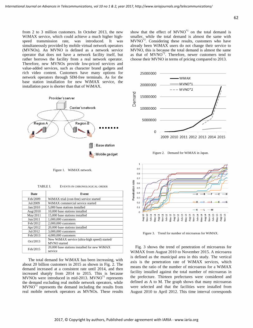
from 2 to 3 million customers. In October 2013, the new WiMAX service, which could achieve a much higher high-speed transmission rate, was introduced. It was simultaneously provided by mobile virtual network operators (MVNOs). An MVNO is defined as a network service operator that does not have a network facility itself, but rather borrows the facility from a real network operator. Therefore, new MVNOs provide low-priced services and value-added services, such as character brand gadgets and rich video content. Customers have many options for network operators through SIM-free terminals. As for the base station installation for new WiMAX service, the installation pace is shorter than that of WiMAX.

Figure 1. WiMAX network.

TABLE I. EVENTS IN CHRONOLOGICAL ORDER

Date Event Feb/2009 WiMAX trial (cost-free) service started Jul/2009 WiMAX commercial service started Jan/2010 5,000 base stations installed Aug/2010 10,000 base stations installed May/2011 15,000 base stations installed Jun/2011 1,000,000 customers Feb/2012 2,000,000 customers Apr/2012 20,000 base stations installed Jul/2012 3,000,000 customers Feb/2013 4,000,000 customers

Oct/2013 New WiMAX service (ultra-high speed) started/ MVNO started

Feb/2015 20,000 base stations installed for new WiMAX service

The total demand for WiMAX has been increasing, with

about 20 billion customers in 2015 as shown in Fig. 2. The demand increased at a consistent rate until 2014, and then increased sharply from 2014 to 2015. This is because MVNOs were introduced in mid-2013. MVNO*1 represents the demand excluding real mobile network operators, while MVNO*2 represents the demand including the results from real mobile network operators as MVNOs. These results

show that the effect of MVNO*1 on the total demand is smaller, while the total demand is almost the same with MVNO*2. Considering these results, customers who have already been WiMAX users do not change their service to MVNO, this is because the total demand is almost the same as that of MVNO*2. Therefore, newer customers tend to choose their MVNO in terms of pricing compared to 2013.

Figure 2. Demand for WiMAX in Japan.

Figure 3. Trend for number of microareas for WiMAX.

Fig. 3 shows the trend of penetration of microareas for

WiMAX from August 2010 to November 2015. A microarea is defined as the municipal area in this study. The vertical axis is the penetration rate of WiMAX services, which means the ratio of the number of microareas for a WiMAX facility installed against the total number of microareas in the prefecture. Thirteen prefectures were considered and defined as A to M. The graph shows that many microareas were selected and that the facilities were installed from August 2010 to April 2012. This time interval corresponds

62



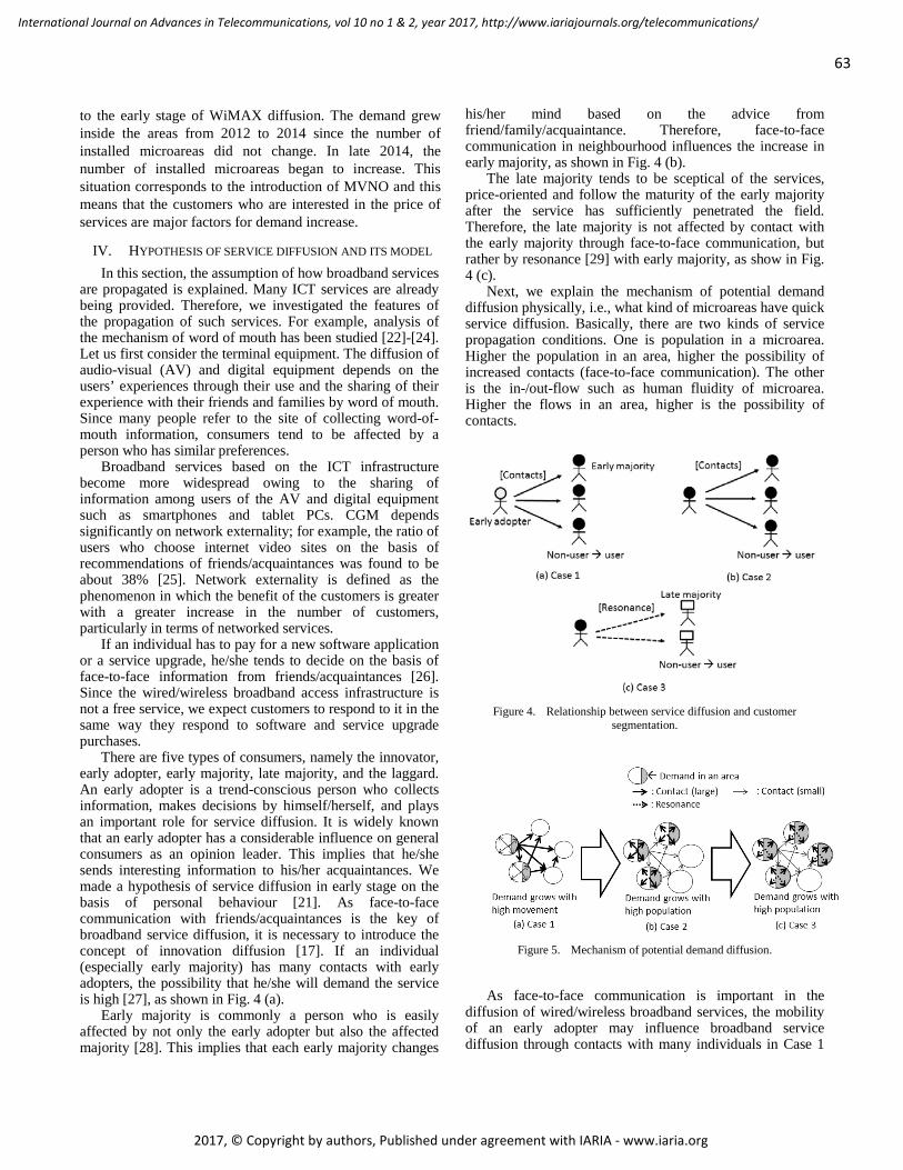
to the early stage of WiMAX diffusion. The demand grew inside the areas from 2012 to 2014 since the number of installed microareas did not change. In late 2014, the number of installed microareas began to increase. This situation corresponds to the introduction of MVNO and this means that the customers who are interested in the price of services are major factors for demand increase.

IV. HYPOTHESIS OF SERVICE DIFFUSION AND ITS MODEL In this section, the assumption of how broadband services

are propagated is explained. Many ICT services are already being provided. Therefore, we investigated the features of the propagation of such services. For example, analysis of the mechanism of word of mouth has been studied [22]-[24]. Let us first consider the terminal equipment. The diffusion of audio-visual (AV) and digital equipment depends on the users’ experiences through their use and the sharing of their experience with their friends and families by word of mouth. Since many people refer to the site of collecting word-of-mouth information, consumers tend to be affected by a person who has similar preferences.

Broadband services based on the ICT infrastructure become more widespread owing to the sharing of information among users of the AV and digital equipment such as smartphones and tablet PCs. CGM depends significantly on network externality; for example, the ratio of users who choose internet video sites on the basis of recommendations of friends/acquaintances was found to be about 38% [25]. Network externality is defined as the phenomenon in which the benefit of the customers is greater with a greater increase in the number of customers, particularly in terms of networked services.

If an individual has to pay for a new software application or a service upgrade, he/she tends to decide on the basis of face-to-face information from friends/acquaintances [26]. Since the wired/wireless broadband access infrastructure is not a free service, we expect customers to respond to it in the same way they respond to software and service upgrade purchases.

There are five types of consumers, namely the innovator, early adopter, early majority, late majority, and the laggard. An early adopter is a trend-conscious person who collects information, makes decisions by himself/herself, and plays an important role for service diffusion. It is widely known that an early adopter has a considerable influence on general consumers as an opinion leader. This implies that he/she sends interesting information to his/her acquaintances. We made a hypothesis of service diffusion in early stage on the basis of personal behaviour [21]. As face-to-face communication with friends/acquaintances is the key of broadband service diffusion, it is necessary to introduce the concept of innovation diffusion [17]. If an individual (especially early majority) has many contacts with early adopters, the possibility that he/she will demand the service is high [27], as shown in Fig. 4 (a).

Early majority is commonly a person who is easily affected by not only the early adopter but also the affected majority [28]. This implies that each early majority changes

his/her mind based on the advice from friend/family/acquaintance. Therefore, face-to-face communication in neighbourhood influences the increase in early majority, as shown in Fig. 4 (b).

The late majority tends to be sceptical of the services, price-oriented and follow the maturity of the early majority after the service has sufficiently penetrated the field. Therefore, the late majority is not affected by contact with the early majority through face-to-face communication, but rather by resonance [29] with early majority, as show in Fig. 4 (c).

Next, we explain the mechanism of potential demand diffusion physically, i.e., what kind of microareas have quick service diffusion. Basically, there are two kinds of service propagation conditions. One is population in a microarea. Higher the population in an area, higher the possibility of increased contacts (face-to-face communication). The other is the in-/out-flow such as human fluidity of microarea. Higher the flows in an area, higher is the possibility of contacts.

Figure 4. Relationship between service diffusion and customer

segmentation.

Figure 5. Mechanism of potential demand diffusion.

As face-to-face communication is important in the

diffusion of wired/wireless broadband services, the mobility of an early adopter may influence broadband service diffusion through contacts with many individuals in Case 1

63



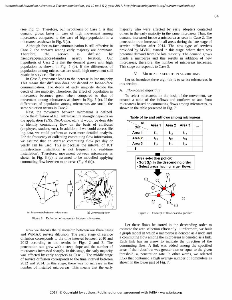
(see Fig. 5). Therefore, our hypothesis of Case 1 is that demand grows faster in case of high movement among microareas compared to the case of high population in a microarea, as shown in Fig. 5 (a).

Although face-to-face communication is still effective in Case 2, the contacts among early majority are dominant. Therefore, the service is diffused by friends/acquaintances/families nearby location. Our hypothesis of Case 2 is that the demand grows with high population as shown in Fig. 5 (b). If the differences of population among microareas are small, high movement still results in service diffusion.

In Case 3, resonance leads to the increase in late majority. This means that diffusion does not depend on face-to-face communication. The deeds of early majority decide the deeds of late majority. Therefore, the effect of population in microareas becomes great when compared to that of movement among microareas as shown in Fig. 5 (c). If the differences of population among microareas are small, the same situation occurs in Case 2.

Next, the movement between microareas is defined. Since the diffusion of ICT infrastructure strongly depends on the application (SNS, Net-Game, etc.), it would be desirable to identify commuting flow on the basis of attributes (employee, student, etc.). In addition, if we could access life log data, we could perform an even more detailed analysis. For the frequency of collecting commuting flow information, we assume that an average commuting flow per day or yearly can be used. This is because the interval of ICT infrastructure installation is not frequent (no real-time installation). Therefore, movement between microareas as shown in Fig. 6 (a) is assumed to be modelled applying commuting flow between microareas (Fig. 6 (b)).

Figure 6. Definition of movement between microareas.

Now we discuss the relationship between our three cases

and WiMAX service diffusion. The early stage of service diffusion corresponds to the time interval between 2010 and 2012 according to the results in Figs. 2 and 3. The penetration rate grew with a steep slope and the number of microareas increased sharply. In this stage, the early majority was affected by early adopters as Case 1. The middle stage of service diffusion corresponds to the time interval between 2012 and 2014. In this stage, there was no increase in the number of installed microareas. This means that the early

majority who were affected by early adopters contacted others in the early majority in the same microarea. Thus, the demand increased inside a microarea as seen in Case 2. The penetration rate increased in all areas during the late stage of service diffusion after 2014. The new type of services provided by MVNO started in this stage, where there was potential demand from the late majority. The demand grows inside a microarea and this results in addition of new microareas, therefore, the number of micoareas increases. This stage corresponds to Case 3.

V. MICROAREA SELECTION ALGORITHMS Let us introduce three algorithms to select microareas in

this section.

A. Flow-based algorithm To select microareas on the basis of the movement, we

created a table of the inflows and outflows to and from microareas based on commuting flows among microareas, as shown in the table presented in Fig. 7.

Figure 7. Concept of flow-based algorithm.

Let these flows be sorted in the descending order to

estimate the area selection efficiently. Furthermore, we built a graph model in which a microarea is denoted as a node and a commuting flow among the microareas is denoted as a link. Each link has an arrow to indicate the direction of the commuting flow. A link was added among the specified areas if the in/outflow was greater than or equal to the given threshold, α, penetration rate. In other words, we selected links that contained a high average number of commuters as shown in the lower part of Fig. 7.

64



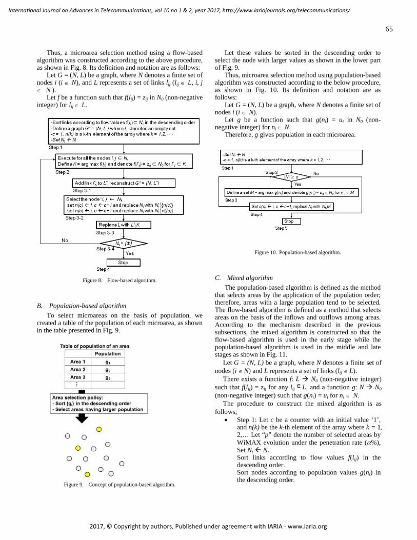
Thus, a microarea selection method using a flow-based algorithm was constructed according to the above procedure, as shown in Fig. 8. Its definition and notation are as follows:

Let G = (N, L) be a graph, where N denotes a finite set of nodes i (i ∈ N), and L represents a set of links lij (lij ∈ L, i, j ∈ N ).

Let f be a function such that f(lij) = zij in N0 (non-negative integer) for lij ∈ L.

Figure 8. Flow-based algorithm.

B. Population-based algorithm To select microareas on the basis of population, we

created a table of the population of each microarea, as shown in the table presented in Fig. 9.

Figure 9. Concept of population-based algorithm.

Let these values be sorted in the descending order to select the node with larger values as shown in the lower part of Fig. 9.

Thus, microarea selection method using population-based algorithm was constructed according to the below procedure, as shown in Fig. 10. Its definition and notation are as follows:

Let G = (N, L) be a graph, where N denotes a finite set of nodes i (i ∈ N).

Let g be a function such that g(ni) = ui in N0 (non-negative integer) for ni ∈ N.

Therefore, g gives population in each microarea.

Figure 10. Population-based algorithm.

C. Mixed algorithm The population-based algorithm is defined as the method

that selects areas by the application of the population order; therefore, areas with a large population tend to be selected. The flow-based algorithm is defined as a method that selects areas on the basis of the inflows and outflows among areas. According to the mechanism described in the previous subsections, the mixed algorithm is constructed so that the flow-based algorithm is used in the early stage while the population-based algorithm is used in the middle and late stages as shown in Fig. 11.

Let G = (N, L) be a graph, where N denotes a finite set of nodes (i ∈ N) and L represents a set of links (lij ∈ L).

There exists a function f: L N0 (non-negative integer) such that f(lij) = zij for any lij L, and a function g: N N0 (non-negative integer) such that g(ni) = ui for ni ∈ N.

The procedure to construct the mixed algorithm is as follows;

• Step 1: Let c be a counter with an initial value ‘1’, and n(k) be the k-th element of the array where k = 1, 2,… Let “p” denote the number of selected areas by WiMAX evolution under the penetration rate (α%), Set Nt N. Sort links according to flow values f(lij) in the descending order. Sort nodes according to population values g(ni) in the descending order.

65



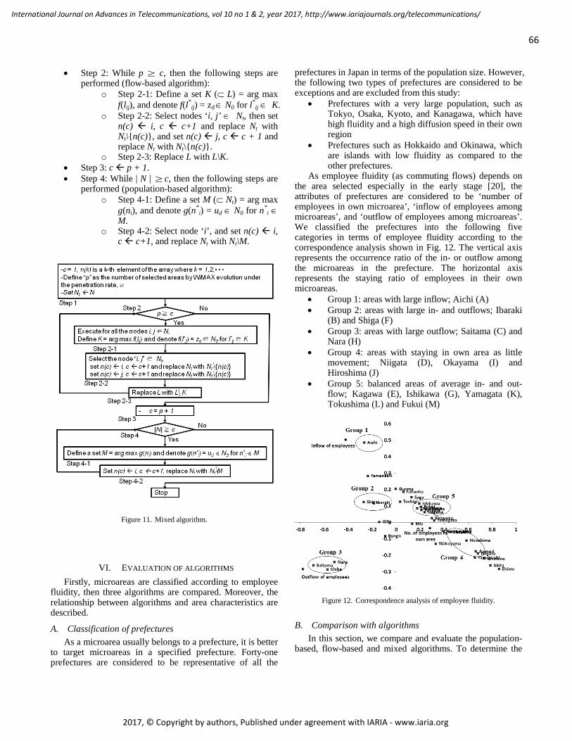
• Step 2: While p ≥ c, then the following steps are performed (flow-based algorithm):

o Step 2-1: Define a set K (⊂ L) = arg max f(lij), and denote f(l*ij) = zd ∈ N0 for l*

ij ∈ K. o Step 2-2: Select nodes ‘i, j’ ∈ Nt, then set

n(c) i, c c+1 and replace Nt with Nt\{n(c)}, and set n(c) j, c c + 1 and replace Nt with Nt\{n(c)}.

o Step 2-3: Replace L with L\K. • Step 3: c p + 1. • Step 4: While | N | ≥ c, then the following steps are

performed (population-based algorithm): o Step 4-1: Define a set M (⊂ Nt) = arg max

g(ni), and denote g(n*i) = ud ∈ N0 for n*

i ∈ M.

o Step 4-2: Select node ‘i’, and set n(c) i, c c+1, and replace Nt with Nt\M.

Figure 11. Mixed algorithm.

VI. EVALUATION OF ALGORITHMS Firstly, microareas are classified according to employee

fluidity, then three algorithms are compared. Moreover, the relationship between algorithms and area characteristics are described.

A. Classification of prefectures As a microarea usually belongs to a prefecture, it is better

to target microareas in a specified prefecture. Forty-one prefectures are considered to be representative of all the

prefectures in Japan in terms of the population size. However, the following two types of prefectures are considered to be exceptions and are excluded from this study:

• Prefectures with a very large population, such as Tokyo, Osaka, Kyoto, and Kanagawa, which have high fluidity and a high diffusion speed in their own region

• Prefectures such as Hokkaido and Okinawa, which are islands with low fluidity as compared to the other prefectures.

As employee fluidity (as commuting flows) depends on the area selected especially in the early stage [20], the attributes of prefectures are considered to be ‘number of employees in own microarea’, ‘inflow of employees among microareas’, and ‘outflow of employees among microareas’. We classified the prefectures into the following five categories in terms of employee fluidity according to the correspondence analysis shown in Fig. 12. The vertical axis represents the occurrence ratio of the in- or outflow among the microareas in the prefecture. The horizontal axis represents the staying ratio of employees in their own microareas.

• Group 1: areas with large inflow; Aichi (A) • Group 2: areas with large in- and outflows; Ibaraki

(B) and Shiga (F) • Group 3: areas with large outflow; Saitama (C) and

Nara (H) • Group 4: areas with staying in own area as little

movement; Niigata (D), Okayama (I) and Hiroshima (J)

• Group 5: balanced areas of average in- and out-flow; Kagawa (E), Ishikawa (G), Yamagata (K), Tokushima (L) and Fukui (M)

Figure 12. Correspondence analysis of employee fluidity.

B. Comparison with algorithms In this section, we compare and evaluate the population-

based, flow-based and mixed algorithms. To determine the

66



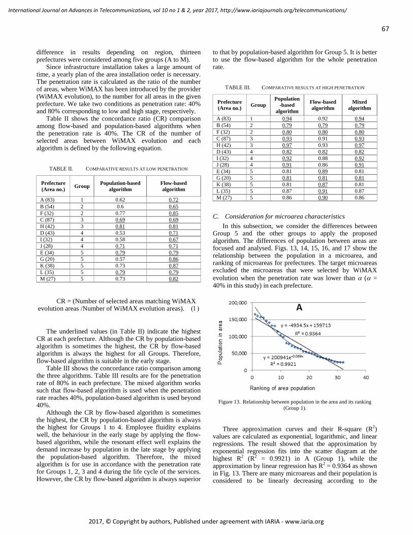
difference in results depending on region, thirteen prefectures were considered among five groups (A to M).

Since infrastructure installation takes a large amount of time, a yearly plan of the area installation order is necessary. The penetration rate is calculated as the ratio of the number of areas, where WiMAX has been introduced by the provider (WiMAX evolution), to the number for all areas in the given prefecture. We take two conditions as penetration rate: 40% and 80% corresponding to low and high stage, respectively.

Table II shows the concordance ratio (CR) comparison among flow-based and population-based algorithms when the penetration rate is 40%. The CR of the number of selected areas between WiMAX evolution and each algorithm is defined by the following equation.

TABLE II. COMPARATIVE RESULTS AT LOW PENETRATION

Prefecture (Area no.) Group Population-based

algorithm Flow-based algorithm

A (83) 1 0.62 B (54)

0.72 2 0.6

F (32) 0.65

2 0.77 C (87)

0.85 3 0.69

H (42) 0.69

3 0.81 D (43)

0.81 4 0.53

I (32) 0.71

4 0.58 J (28)

0.67 4 0.71

E (34) 0.71

5 0.79 G (20)

0.79 5 0.57

K (38) 0.86

5 0.73 L (35)

0.87 5 0.79

M (27) 0.79

5 0.73

0.82

CR = (Number of selected areas matching WiMAX evolution areas /Number of WiMAX evolution areas). (1)

The underlined values (in Table II) indicate the highest

CR at each prefecture. Although the CR by population-based algorithm is sometimes the highest, the CR by flow-based algorithm is always the highest for all Groups. Therefore, flow-based algorithm is suitable in the early stage.

Table III shows the concordance ratio comparison among the three algorithms. Table III results are for the penetration rate of 80% in each prefecture. The mixed algorithm works such that flow-based algorithm is used when the penetration rate reaches 40%, population-based algorithm is used beyond 40%.

Although the CR by flow-based algorithm is sometimes the highest, the CR by population-based algorithm is always the highest for Groups 1 to 4. Employee fluidity explains well, the behaviour in the early stage by applying the flow-based algorithm, while the resonant effect well explains the demand increase by population in the late stage by applying the population-based algorithm. Therefore, the mixed algorithm is for use in accordance with the penetration rate for Groups 1, 2, 3 and 4 during the life cycle of the services. However, the CR by flow-based algorithm is always superior

to that by population-based algorithm for Group 5. It is better to use the flow-based algorithm for the whole penetration rate.

TABLE III. COMPARATIVE RESULTS AT HIGH PENETRATION

Prefecture (Area no.) Group

Population-based

algorithm

Flow-based algorithm

Mixed algorithm

A (83) 1 0.92 0.94 B (54)

0.94 2 0.79 0.79

F (32) 0.79

2 0.80 0.80 C (87)

0.80 3 0.91 0.93

H (42) 0.93

3 0.93 0.97 D (43)

0.97 4 0.82 0.82

I (32) 0.82

4 0.88 0.92 J (28)

0.92 4 0.86 0.91

E (34) 0.91

5 0.81 0.81 0.89 G (20) 5 0.81 0.81 K (38)

0.81 5 0.81 0.81 0.87

L (35) 5 0.87 0.87 0.91 M (27) 5 0.86 0.86 0.90

C. Consideration for microarea characteristics In this subsection, we consider the differences between

Group 5 and the other groups to apply the proposed algorithm. The differences of population between areas are focused and analysed. Figs. 13, 14, 15, 16, and 17 show the relationship between the population in a microarea, and ranking of microareas for prefectures. The target microareas excluded the microareas that were selected by WiMAX evolution when the penetration rate was lower than α (α = 40% in this study) in each prefecture.

Figure 13. Relationship between population in the area and its ranking

(Group 1).

Three approximation curves and their R-square (R2)

values are calculated as exponential, logarithmic, and linear regressions. The result showed that the approximation by exponential regression fits into the scatter diagram at the highest R2 (R2 = 0.9921) in A (Group 1), while the approximation by linear regression has R2 = 0.9364 as shown in Fig. 13. There are many microareas and their population is considered to be linearly decreasing according to the

67



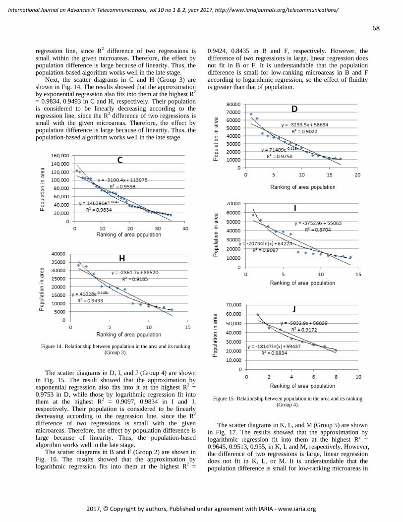
regression line, since R2 difference of two regressions is small within the given microareas. Therefore, the effect by population difference is large because of linearity. Thus, the population-based algorithm works well in the late stage.

Next, the scatter diagrams in C and H (Group 3) are shown in Fig. 14. The results showed that the approximation by exponential regression also fits into them at the highest R2 = 0.9834, 0.9493 in C and H, respectively. Their population is considered to be linearly decreasing according to the regression line, since the R2 difference of two regressions is small with the given microareas. Therefore, the effect by population difference is large because of linearity. Thus, the population-based algorithm works well in the late stage.


(Group 3).

The scatter diagrams in D, I, and J (Group 4) are shown

in Fig. 15. The result showed that the approximation by exponential regression also fits into it at the highest R2 = 0.9753 in D, while those by logarithmic regression fit into them at the highest R2 = 0.9097, 0.9834 in I and J, respectively. Their population is considered to be linearly decreasing according to the regression line, since the R2 difference of two regressions is small with the given microareas. Therefore, the effect by population difference is large because of linearity. Thus, the population-based algorithm works well in the late stage.

The scatter diagrams in B and F (Group 2) are shown in Fig. 16. The results showed that the approximation by logarithmic regression fits into them at the highest R2 =

0.9424, 0.8435 in B and F, respectively. However, the difference of two regressions is large, linear regression does not fit in B or F. It is understandable that the population difference is small for low-ranking microareas in B and F according to logarithmic regression, so the effect of fluidity is greater than that of population.


(Group 4).

The scatter diagrams in K, L, and M (Group 5) are shown

in Fig. 17. The results showed that the approximation by logarithmic regression fit into them at the highest R2 = 0.9645, 0.9513, 0.955, in K, L and M, respectively. However, the difference of two regressions is large, linear regression does not fit in K, L, or M. It is understandable that the population difference is small for low-ranking microareas in

68



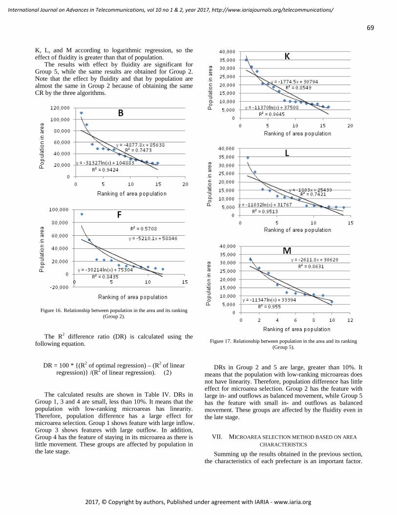
K, L, and M according to logarithmic regression, so the effect of fluidity is greater than that of population.

The results with effect by fluidity are significant for Group 5, while the same results are obtained for Group 2. Note that the effect by fluidity and that by population are almost the same in Group 2 because of obtaining the same CR by the three algorithms.


(Group 2).

The R2 difference ratio (DR) is calculated using the

following equation.

DR = 100 * {(R2 of optimal regression) – (R2 of linear regression)} /(R2 of linear regression). (2)

The calculated results are shown in Table IV. DRs in

Group 1, 3 and 4 are small, less than 10%. It means that the population with low-ranking microareas has linearity. Therefore, population difference has a large effect for microarea selection. Group 1 shows feature with large inflow. Group 3 shows features with large outflow. In addition, Group 4 has the feature of staying in its microarea as there is little movement. These groups are affected by population in the late stage.


(Group 5).

DRs in Group 2 and 5 are large, greater than 10%. It

means that the population with low-ranking microareas does not have linearity. Therefore, population difference has little effect for microarea selection. Group 2 has the feature with large in- and outflows as balanced movement, while Group 5 has the feature with small in- and outflows as balanced movement. These groups are affected by the fluidity even in the late stage.

VII. MICROAREA SELECTION METHOD BASED ON AREA CHARACTERISTICS

Summing up the results obtained in the previous section, the characteristics of each prefecture is an important factor.

69



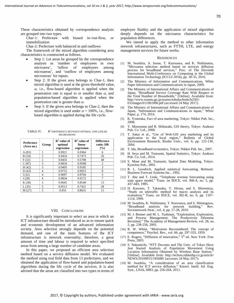
These characteristics obtained by correspondence analysis are grouped into two types.

Char-1: Prefecture with biased in-/out-flow, or immobilization Char-2: Prefecture with balanced in and outflows The framework of the mixed algorithm considering area

characteristics is constructed as follows. • Step 1: Let areas be grouped by the correspondence

analysis as ‘number of employees in own microarea’, ‘inflow of employees among microareas’, and ‘outflow of employees among microareas’ for inputs.

• Step 2: If the given area belongs to Char-1, then mixed algorithm is used at the given threshold value, α, i.e., flow-based algorithm is applied when the penetration rate is equal to or smaller than α, and population-based algorithm is applied when the penetration rate is greater than α.

• Step 3: If the given area belongs to Char-2, then the mixed algorithm is used under α = 100%, i.e., flow-based algorithm is applied during the life cycle.

TABLE IV. R2-DIFFERENCE BETWEEN OPTIMAL AND LINEAR REGRESSIONS

Prefecture (Area no.) Group

R2 value of optimal

regression

R2 value of linear

regression

Difference ratio: DR

(%) A (83) 1 0.9921 0.9364 6 B (54) 2 0.9424 0.7473 26 F (32) 2 0.8435 0.5708 48 C (87) 3 0.9834 0.9598 2 H (42) 3 0.9493 0.9185 3 D (43) 4 0.9753 0.9023 8 I (32) 4 0.9097 0.8704 5 J (28) 4 0.9834 0.9172 7 K (38) 5 0.9645 0.8549 13 L (35) 5 0.9513 0.7421 28 M (27) 5 0.955 0.8631 11

VIII. CONCLUSIONS It is significantly important to select an area in which an

ICT infrastructure should be introduced so as to ensure quick and economic development of an advanced information society. Area selection strongly depends on the potential demand, and one of the main features of the ICT infrastructure is network externality; therefore, a great amount of time and labour is required to select specified areas from among a large number of candidate areas.

In this paper, we proposed an efficient area selection method based on a service diffusion model. We evaluated the method using real field data from 13 prefectures, and we obtained the application of flow-based and population-based algorithms during the life cycle of the services. It is also advised that the areas are classified into two types in terms of

employee fluidity and the application of mixed algorithm deeply depends on the microarea characteristics for population differences.

We intend to apply the method to other information network infrastructures, such as FTTH, LTE, and energy management services for future works.

REFERENCES [1] M. Iwashita, A. Inoue, T. Kurosawa, and K. Nishimatsu,

“Microarea selection method based on services diffusion process for broadband services,” Proc. of The Eleventh International Multi-Conference on Computing in the Global Information Technology (ICCGI 2016), pp. 30-35, 2016.

[2] The Ministry of Information and Communications, White Paper Information and Communications in Japan, 2009.

[3] The Ministry of International Affairs and Communications of Japan, “Broadband Service Coverage Rate With Respect to the Total Number of Households,” [Online]. Available from: http://www.soumu.go.jp/soutsu/tohoku/hodo/h2501-03/images/0110b1006.pdf (accessed 24 May 2017).

[4] The Ministry of International Affairs and Communications of Japan, “Information and Communications in Japan,” White Paper, p. 174, 2014.

[5] K. Yonetaka, Fact of area marketing, Tokyo: Nikkei Pub. Inc., 2008.

[6] Y. Murayama and R. Shibazaki, GIS theory, Tokyo: Asakura Pub. Co. Ltd., 2008.

[7] T. Sakai et al., “Use of Web-GIS area marketing and its application to the local region,” Bulletin of Global Environment Research, Rissho Univ., vol. 6, pp. 125-130, 2004.

[8] T. Ida, Broadband economics, Tokyo: Nikkei Pub. Inc., 2007. [9] H. Seya and M. Tsutsumi, Spatial Statistics, Tokyo: Asakura

Pub. Co. Ltd., 2014. [10] S. Mase and M. Tsutsumi, Spatial Data Modeling, Tokyo:

Kyoritsu Pub., 2001. [11] R. L. Goodrich, Applied statistical forecasting, Belmont:

Business Forecast Systems Inc., 1992. [12] T. Abe and T. Ueda, “Telephone revenue forecasting using

state space model,” Trans. on IEICE, vol. J68-A, no. 5, pp. 437-443, 1985.

[13] H. Kawano, T. Takanaka, Y. Hiruta, and S. Shinomiya, “Study on teletraffic method for macro analysis and its evaluation,” Trans. on IEICE, vol. J82-B, no. 6, pp. 1107-1114, 1999.

[14] M. Iwashita, K. Nishimatsu, T. Kurosawa, and S. Shimogawa, “Broadband analysis for network building,” Rev. Socionetwork Strat., vol. 4, pp. 17-28, 2010.

[15] M. J. Benner and M. L. Tushman, “Exploitation, Exploration, and Process Management: The Productivity Dilemma Revisited,” The Academy of Management Review, vol. 28, no. 2, pp. 238-256, 2003.

[16] R. W. White, “Motivation Reconsidered: The concept of competence,” Psychol. Rev., vol. 66, pp. 297-333, 1959.

[17] E. Rogers, “Diffusion of innovation,” 5th ed. New York: Free Press, 2003.

[18] S. Nakamichi, “NTT Docomo and The Univ. of Tokyo Have Just Started Analysis of Population Movement Using Location Information Obtained by Wireless Base Station,” [Online]. Available from: http://techon.nikkeibp.co.jp/article/ NEWS/20100915/185680/ (accesses 24 May 2017).

[19] M. Iwashita, “A consideration of an area classification method for ICT service diffusion,” Knowl. Intell. Inf. Eng. Syst., LNAI, 6883, pp. 256-264, 2011.

70



[20] M. Iwashita, A. Inoue, T. Kurosawa, and K. Nishimatsu, “Micro area selection framework for ICT infrastructure diffusion based on commuting flow,” Int. J. Comp. Inf. Sci., vol. 13, no. 2, pp. 10-19, 2012.

[21] M. Iwashita, A. Inoue, T. Kurosawa, and K. Nishimatsu, “Efficient microarea selection algorithm for infrastructure installation of broadband services,” Int. J. Comput. Intell. Stud., Inderscience publishers, Vol. 5, Nos 3/4, pp. 29-236, 2017.

[22] K. Ikeda, “The Diffusion of Innovation Through Word-Of-Mouth and Social Networks: A social Psychological Study Combining Snowball Surveys and Multi-Agent Simulation,” Tokyo: Univ. of Tokyo Press, 2010.

[23] S. P. A. T. Dentsu, “How to Create an Atmosphere to Make You Feel Buying,” Tokyo: Diamond Inc., 2007.

[24] H. Katahira, “New theory AIDEES like big tidal stream,” Diamond Visionary, vol. 42, no. 7, pp. 34-37, 2006.

[25] Macromill, “Field Survey of Using Internet Video Site”. [Online]. Available from: http://monitor.macromill.com/

researchdata/20070701movie/index.html (accessed 24 May 2017).

[26] “The Institute for Information and Communications Policy, Research Study of Determinative Factors for Internet Usage and Reality of Use” Tokyo: The Institute for Information and Communications Policy, 2009.

[27] S. Shimogawa and M. Iwashita, “Method for analyzing sociodynamics of telecommunication-based services,” Proc. of 9th IEEE/ACIS International Conference on Computer and Information Science, pp. 99-104, 2010.

[28] G. A. Moor, “Crossing the chasm: Marketing and selling high-tech goods to mainstream customers,” New York: Harper Business, 1991.

[29] Y. Ohsawa, M. Matsumura, and K. Takahashi, “Resonance without Response: The Way of Topic Growth in Communication,” Chance Discov. Real World Decis. Making, Stud. Comput. Intell., Vol. 30, pp. 155-165, 2006.

71



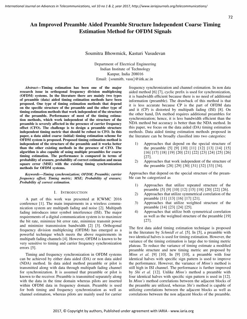
An Improved Preamble Aided Preamble Structure Independent Coarse TimingEstimation Method for OFDM Signals

Soumitra Bhowmick, Kasturi Vasudevan

Department of Electrical EngineeringIndian Institute of Technology

Kanpur, India 208016Email: {soumitb, vasu}@iitk.ac.in

Abstract—Timing estimation has been one of the majorresearch issue in orthogonal frequency division multiplexing(OFDM) systems. In the literature there are mainly two typesof preamble (data) aided timing estimation methods have beenproposed. One type of timing estimation methods that dependon the specific structure of the preamble and the other type oftiming estimation methods that work independent of the structureof the preamble. Performance of most of the timing estima-tion methods, which work independent of the structure of thepreamble is severely affected in the presence of carrier frequencyoffset (CFO). The challenge is to design a preamble structureindependent timing metric that should be robust to CFO. In thispaper, a data aided coarse (initial) timing estimation scheme forOFDM system is proposed. Proposed timing estimation method isindependent of the structure of the preamble and it works betterthan the other existing methods in the presence of CFO. Thealgorithm is also capable of using multiple preambles for coarsetiming estimation. The performance is compared in terms ofprobability of erasure, probability of correct estimation and meansquare error (MSE) with the existing timing synchronizationmethods for OFDM systems.

Keywords—Timing synchronization; OFDM; Preamble; carrierfrequency offset; Timing metric; MSE; Probability of erasure;Probability of correct estimation.

I. INTRODUCTION

A part of this work was presented at ICWMC 2016conference [1]. The main impairments in a wireless commu-nication system are multipath fading and noise [2]. Multipathfading introduces inter symbol interference (ISI). The majorrequirements of a digital communication system is to maximizethe bit rate, minimize bit error rate, minimize transmit powerand minimize transmission bandwidth [2] [3]. Orthogonalfrequency division multiplexing (OFDM) has emerged as apowerful technique which meets the above requirements inmultipath fading channels [4]. However, OFDM is known to bevery sensitive to timing and carrier frequency synchronizationerrors [5].

Timing and frequency synchronization in OFDM systemscan be achieved by either data aided (DA) or non data aided(NDA) method. In data aided method preamble or pilot istransmitted along with data through multipath fading channelfor synchronization. It is assumed that preamble or pilot isknown to the receiver. Preamble is transmitted separately alongwith the data in the time domain whereas pilots are insertedwithin OFDM data in frequency domain. Preamble is usedfor both timing and frequency synchronization as well aschannel estimation, whereas pilots are mainly used for carrier

frequency synchronization and channel estimation. In non dataaided method [6] [7], cyclic prefix is used for synchronization,it is bandwidth efficient because there is no need of additionalinformation (preamble). The drawback of this method is thatit is less accurate because CP is the part of OFDM dataand it (CP) is distorted by multipath fading (ISI) [8]. Onthe other hand, DA method requires additional preambles forsynchronization; hence, it is less bandwidth efficient than theNDA method but accuracy is better than the NDA method. Inthis paper, we focus on the data aided (DA) timing estimationmethods. Data aided timing estimation methods proposed inthe literature can be broadly classified into two categories:

1) Approaches that depend on the special structure ofthe preamble [5] [9] [10] [11] [12] [13] [14] [15][16] [17] [18] [19] [20] [21] [22] [23] [24] [25] [26][27].

2) Approaches that work independent of the structure ofthe preamble [28] [29] [30] [31] [32] [33] [34].

Approaches that depend on the special structure of the pream-ble can be categorized as

1) Approaches that utilize repeated structure of thepreamble [5] [9] [10] [12] [15] [18] [20] [22] [26].

2) Approaches that utilize symmetrical correlation of thepreamble [11] [13] [16] [17] [21].

3) Approaches that utilize weighted structure of thepreamble [14] [23] [24] [25].

4) Approaches that utilize both symmetrical correlationas well as the weighted structure of the preamble [19][27].

The first data aided timing estimation technique is proposedin the literature by Schmidl et al. [5]. In [5], a preamble withtwo identical halves is used for timing estimation. However, thevariance of the timing estimation is large due to timing metricplateau. To reduce the variance of timing estimate a modifiedpreamble structure and new timing metric are proposed byMinn et al. [9] [10]. In [9] [10], a preamble with fouridentical halves with specific sign pattern is used to improvethe performance. However, the variance of Minn’s method isstill high in ISI channel. The performance is further improvedby Shi et al. [12]. Unlike Minn’s method a preamble withfour identical halves with specific sign pattern is used in [12].In Minn’s method correlations between the adjacent blocks ofthe preamble are utilized, whereas Shi’s method is capable ofutilizing correlations between the adjacent blocks as well ascorrelations between the non adjacent blocks of the preamble.

72



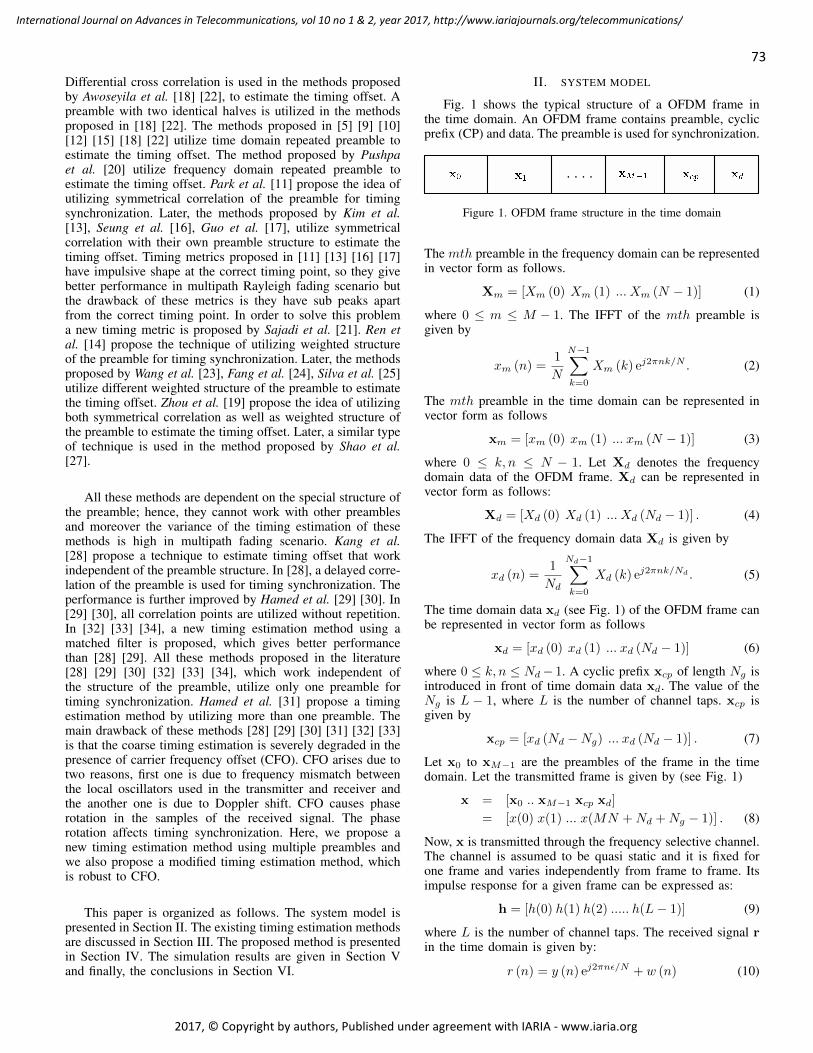
Differential cross correlation is used in the methods proposedby Awoseyila et al. [18] [22], to estimate the timing offset. Apreamble with two identical halves is utilized in the methodsproposed in [18] [22]. The methods proposed in [5] [9] [10][12] [15] [18] [22] utilize time domain repeated preamble toestimate the timing offset. The method proposed by Pushpaet al. [20] utilize frequency domain repeated preamble toestimate the timing offset. Park et al. [11] propose the idea ofutilizing symmetrical correlation of the preamble for timingsynchronization. Later, the methods proposed by Kim et al.[13], Seung et al. [16], Guo et al. [17], utilize symmetricalcorrelation with their own preamble structure to estimate thetiming offset. Timing metrics proposed in [11] [13] [16] [17]have impulsive shape at the correct timing point, so they givebetter performance in multipath Rayleigh fading scenario butthe drawback of these metrics is they have sub peaks apartfrom the correct timing point. In order to solve this problema new timing metric is proposed by Sajadi et al. [21]. Ren etal. [14] propose the technique of utilizing weighted structureof the preamble for timing synchronization. Later, the methodsproposed by Wang et al. [23], Fang et al. [24], Silva et al. [25]utilize different weighted structure of the preamble to estimatethe timing offset. Zhou et al. [19] propose the idea of utilizingboth symmetrical correlation as well as weighted structure ofthe preamble to estimate the timing offset. Later, a similar typeof technique is used in the method proposed by Shao et al.[27].

All these methods are dependent on the special structure ofthe preamble; hence, they cannot work with other preamblesand moreover the variance of the timing estimation of thesemethods is high in multipath fading scenario. Kang et al.[28] propose a technique to estimate timing offset that workindependent of the preamble structure. In [28], a delayed corre-lation of the preamble is used for timing synchronization. Theperformance is further improved by Hamed et al. [29] [30]. In[29] [30], all correlation points are utilized without repetition.In [32] [33] [34], a new timing estimation method using amatched filter is proposed, which gives better performancethan [28] [29]. All these methods proposed in the literature[28] [29] [30] [32] [33] [34], which work independent ofthe structure of the preamble, utilize only one preamble fortiming synchronization. Hamed et al. [31] propose a timingestimation method by utilizing more than one preamble. Themain drawback of these methods [28] [29] [30] [31] [32] [33]is that the coarse timing estimation is severely degraded in thepresence of carrier frequency offset (CFO). CFO arises due totwo reasons, first one is due to frequency mismatch betweenthe local oscillators used in the transmitter and receiver andthe another one is due to Doppler shift. CFO causes phaserotation in the samples of the received signal. The phaserotation affects timing synchronization. Here, we propose anew timing estimation method using multiple preambles andwe also propose a modified timing estimation method, whichis robust to CFO.

This paper is organized as follows. The system model ispresented in Section II. The existing timing estimation methodsare discussed in Section III. The proposed method is presentedin Section IV. The simulation results are given in Section Vand finally, the conclusions in Section VI.

II. SYSTEM MODEL

Fig. 1 shows the typical structure of a OFDM frame inthe time domain. An OFDM frame contains preamble, cyclicprefix (CP) and data. The preamble is used for synchronization.

Figure 1. OFDM frame structure in the time domain

The mth preamble in the frequency domain can be representedin vector form as follows.

Xm = [Xm (0) Xm (1) ... Xm (N − 1)] (1)

where 0 ≤ m ≤ M − 1. The IFFT of the mth preamble isgiven by

xm (n) =1

N

N−1∑k=0

Xm (k) ej2πnk/N . (2)

The mth preamble in the time domain can be represented invector form as follows

xm = [xm (0) xm (1) ... xm (N − 1)] (3)

where 0 ≤ k, n ≤ N − 1. Let Xd denotes the frequencydomain data of the OFDM frame. Xd can be represented invector form as follows:

Xd = [Xd (0) Xd (1) ... Xd (Nd − 1)] . (4)

The IFFT of the frequency domain data Xd is given by

xd (n) =1

Nd

Nd−1∑k=0

Xd (k) ej2πnk/Nd . (5)

The time domain data xd (see Fig. 1) of the OFDM frame canbe represented in vector form as follows

xd = [xd (0) xd (1) ... xd (Nd − 1)] (6)

where 0 ≤ k, n ≤ Nd− 1. A cyclic prefix xcp of length Ng isintroduced in front of time domain data xd. The value of theNg is L − 1, where L is the number of channel taps. xcp isgiven by

xcp = [xd (Nd −Ng) ... xd (Nd − 1)] . (7)

Let x0 to xM−1 are the preambles of the frame in the timedomain. Let the transmitted frame is given by (see Fig. 1)

x = [x0 .. xM−1 xcp xd]

= [x(0) x(1) ... x(MN +Nd +Ng − 1)] . (8)

Now, x is transmitted through the frequency selective channel.The channel is assumed to be quasi static and it is fixed forone frame and varies independently from frame to frame. Itsimpulse response for a given frame can be expressed as:

h = [h(0) h(1) h(2) ..... h(L− 1)] (9)

where L is the number of channel taps. The received signal rin the time domain is given by:

r (n) = y (n) ej2πnε/N + w (n) (10)

73



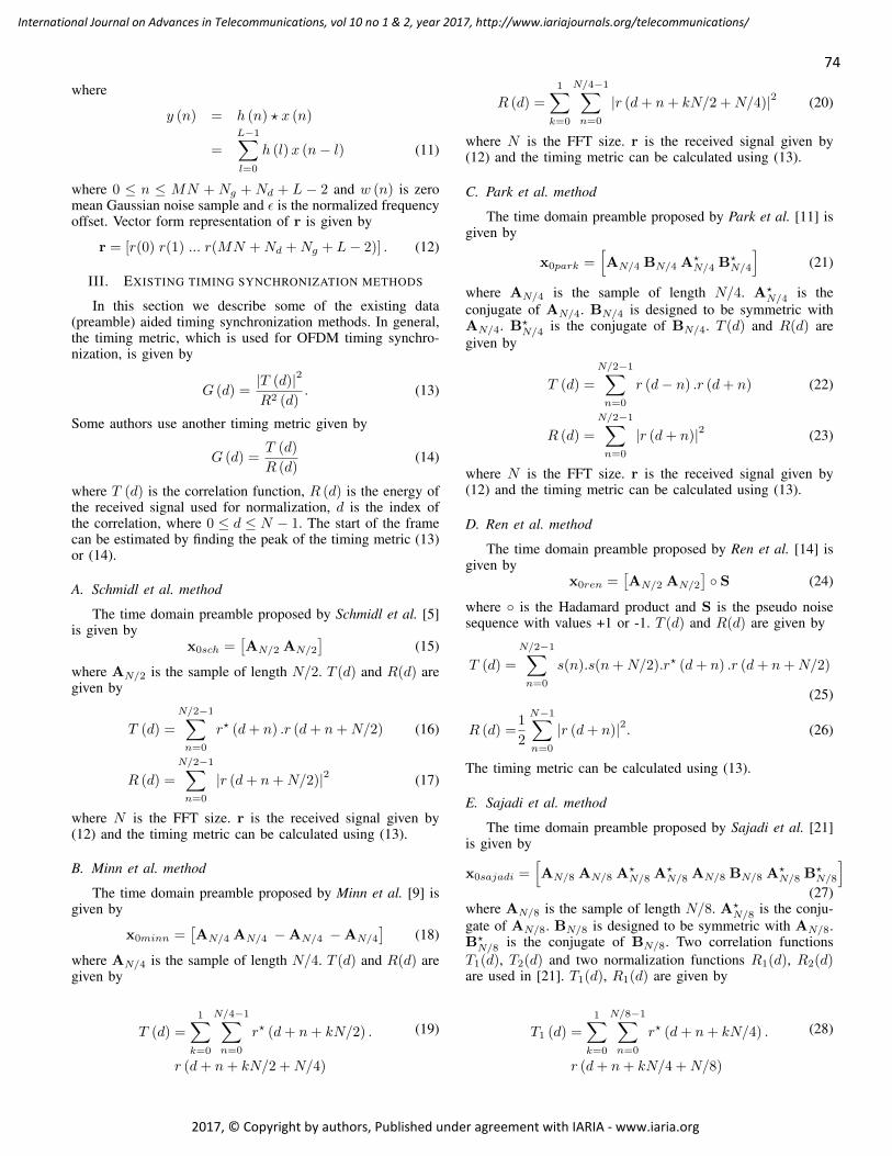
where

y (n) = h (n) ? x (n)

=

L−1∑l=0

h (l)x (n− l) (11)

where 0 ≤ n ≤ MN + Ng + Nd + L − 2 and w (n) is zeromean Gaussian noise sample and ε is the normalized frequencyoffset. Vector form representation of r is given by

r = [r(0) r(1) ... r(MN +Nd +Ng + L− 2)] . (12)

III. EXISTING TIMING SYNCHRONIZATION METHODS

In this section we describe some of the existing data(preamble) aided timing synchronization methods. In general,the timing metric, which is used for OFDM timing synchro-nization, is given by

G (d) =|T (d)|2

R2 (d). (13)

Some authors use another timing metric given by

G (d) =T (d)

R (d)(14)

where T (d) is the correlation function, R (d) is the energy ofthe received signal used for normalization, d is the index ofthe correlation, where 0 ≤ d ≤ N − 1. The start of the framecan be estimated by finding the peak of the timing metric (13)or (14).

A. Schmidl et al. method

The time domain preamble proposed by Schmidl et al. [5]is given by

x0sch =[AN/2 AN/2

](15)

where AN/2 is the sample of length N/2. T (d) and R(d) aregiven by

T (d) =

N/2−1∑n=0

r? (d+ n) .r (d+ n+N/2) (16)

R (d) =

N/2−1∑n=0

|r (d+ n+N/2)|2 (17)

where N is the FFT size. r is the received signal given by(12) and the timing metric can be calculated using (13).

B. Minn et al. method

The time domain preamble proposed by Minn et al. [9] isgiven by

x0minn =[AN/4 AN/4 −AN/4 −AN/4

](18)

where AN/4 is the sample of length N/4. T (d) and R(d) aregiven by

(19)T (d) =

1∑k=0

N/4−1∑n=0

r? (d+ n+ kN/2) .

r (d+ n+ kN/2 +N/4)

R (d) =

1∑k=0

N/4−1∑n=0

|r (d+ n+ kN/2 +N/4)|2 (20)


C. Park et al. method

The time domain preamble proposed by Park et al. [11] isgiven by

x0park =[AN/4 BN/4 A

?N/4 B

?N/4

](21)

where AN/4 is the sample of length N/4. A?N/4 is the

conjugate of AN/4. BN/4 is designed to be symmetric withAN/4. B?

N/4 is the conjugate of BN/4. T (d) and R(d) aregiven by

T (d) =

N/2−1∑n=0

r (d− n) .r (d+ n) (22)

R (d) =

N/2−1∑n=0

|r (d+ n)|2 (23)


D. Ren et al. method

The time domain preamble proposed by Ren et al. [14] isgiven by

x0ren =[AN/2 AN/2

]◦ S (24)

where ◦ is the Hadamard product and S is the pseudo noisesequence with values +1 or -1. T (d) and R(d) are given by

T (d) =

N/2−1∑n=0

s(n).s(n+N/2).r? (d+ n) .r (d+ n+N/2)

(25)

R (d) =1

2

N−1∑n=0

|r (d+ n)|2. (26)

The timing metric can be calculated using (13).

E. Sajadi et al. method

The time domain preamble proposed by Sajadi et al. [21]is given by

x0sajadi =[AN/8 AN/8 A

?N/8 A

?N/8 AN/8 BN/8 A

?N/8 B

?N/8

](27)

where AN/8 is the sample of length N/8. A?N/8 is the conju-

gate of AN/8. BN/8 is designed to be symmetric with AN/8.B?N/8 is the conjugate of BN/8. Two correlation functions

T1(d), T2(d) and two normalization functions R1(d), R2(d)are used in [21]. T1(d), R1(d) are given by

(28)T1 (d) =

1∑k=0

N/8−1∑n=0

r? (d+ n+ kN/4) .

r (d+ n+ kN/4 +N/8)

74



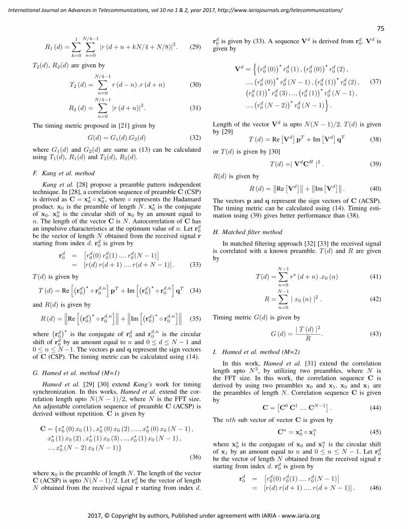
R1 (d) =

1∑k=0

N/4−1∑n=0

|r (d+ n+ kN/4 +N/8)|2. (29)

T2(d), R2(d) are given by

T2 (d) =

N/4−1∑n=0

r (d− n) .r (d+ n) (30)

R2 (d) =

N/4−1∑n=0

|r (d+ n)|2. (31)

The timing metric proposed in [21] given by

G(d) = G1(d).G2(d) (32)

where G1(d) and G2(d) are same as (13) can be calculatedusing T1(d), R1(d) and T2(d), R2(d).

F. Kang et al. method

Kang et al. [28] propose a preamble pattern independenttechnique. In [28], a correlation sequence of preamble C (CSP)is derived as C = x?0 ◦ xn0 , where ◦ represents the Hadamardproduct. x0 is the preamble of length N . x?0 is the conjugateof x0. xn0 is the circular shift of x0 by an amount equal ton. The length of the vector C is N . Autocorrelation of C hasan impulsive characteristics at the optimum value of n. Let rd0be the vector of length N obtained from the received signal rstarting from index d. rd0 is given by

rd0 =[rd0(0) r

d0(1) .... r

d0(N − 1)

]= [r(d) r(d+ 1) .... r(d+N − 1)] . (33)

T (d) is given by

T (d) = Re[(rd0)? ◦ rd,n0

]pT + Im

[(rd0)? ◦ rd,n0

]qT (34)

and R(d) is given by

R (d) =∥∥∥Re

[(rd0)? ◦ rd,n0

]∥∥∥+ ∥∥∥Im[(rd0)? ◦ rd,n0

]∥∥∥ (35)

where(rd0)?

is the conjugate of rd0 and rd,n0 is the circularshift of rd0 by an amount equal to n and 0 ≤ d ≤ N − 1 and0 ≤ n ≤ N−1. The vectors p and q represent the sign vectorsof C (CSP). The timing metric can be calculated using (14).

G. Hamed et al. method (M=1)

Hamed et al. [29] [30] extend Kang’s work for timingsynchronization. In this works, Hamed et al. extend the cor-relation length upto N(N − 1)/2, where N is the FFT size.An adjustable correlation sequence of preamble C (ACSP) isderived without repetition. C is given by

C = {x?0 (0)x0 (1) , x?0 (0)x0 (2) , ..., x?0 (0)x0 (N − 1) ,

x?0 (1)x0 (2) , x?0 (1)x0 (3) , .., x

?0 (1)x0 (N − 1) ,

..., x?0 (N − 2)x0 (N − 1)}(36)

where x0 is the preamble of length N . The length of the vectorC (ACSP) is upto N(N−1)/2. Let rd0 be the vector of lengthN obtained from the received signal r starting from index d.

rd0 is given by (33). A sequence Vd is derived from rd0. Vd isgiven by

(37)

Vd ={(rd0 (0)

)?rd0 (1) ,

(rd0 (0)

)?rd0 (2) ,

...,(rd0 (0)

)?rd0 (N − 1) ,

(rd0 (1)

)?rd0 (2) ,(

rd0 (1))?rd0 (3) , ..,

(rd0 (1)

)?rd0 (N − 1) ,

...,(rd0 (N − 2)

)?rd0 (N − 1)

}.

Length of the vector Vd is upto N(N − 1)/2. T (d) is givenby [29]

T (d) = Re[Vd]pT + Im

[Vd]qT (38)

or T (d) is given by [30]

T (d) =| VdCH |2 . (39)

R(d) is given by

R (d) =∥∥Re

[Vd]∥∥+ ∥∥Im

[Vd]∥∥ . (40)

The vectors p and q represent the sign vectors of C (ACSP).The timing metric can be calculated using (14). Timing esti-mation using (39) gives better performance than (38).

H. Matched filter method

In matched filtering approach [32] [33] the received signalis correlated with a known preamble. T (d) and R are givenby

T (d) =

N−1∑n=0

r? (d+ n) .x0 (n) (41)

R =

N−1∑n=0

| x0 (n) |2 . (42)

Timing metric G(d) is given by

G (d) =| T (d) |2

R. (43)

I. Hamed et al. method (M=2)

In this work, Hamed et al. [31] extend the correlationlength upto N2, by utilizing two preambles, where N isthe FFT size. In this work, the correlation sequence C isderived by using two preambles x0 and x1. x0 and x1 arethe preambles of length N . Correlation sequence C is givenby

C =[C0 C1 ....CN−1

]. (44)

The nth sub vector of vector C is given by

Cn = x?0 ◦ xn1 (45)

where x?0 is the conjugate of x0 and xn1 is the circular shiftof x1 by an amount equal to n and 0 ≤ n ≤ N − 1. Let rd0be the vector of length N obtained from the received signal rstarting from index d. rd0 is given by

rd0 =[rd0(0) r

d0(1) .... r

d0(N − 1)

]= [r(d) r(d+ 1) .... r(d+N − 1)] . (46)

75



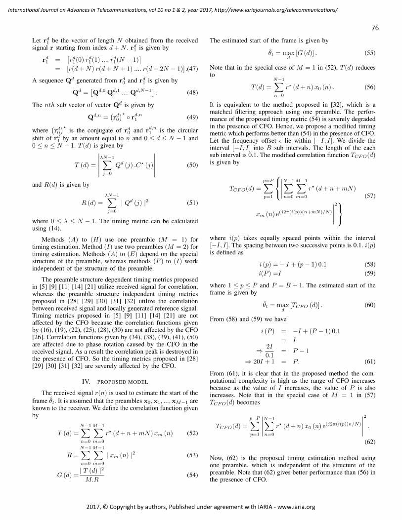
Let rd1 be the vector of length N obtained from the receivedsignal r starting from index d+N . rd1 is given by

rd1 =[rd1(0) r

d1(1) .... r

d1(N − 1)

]= [r(d+N) r(d+N + 1) .... r(d+ 2N − 1)] .(47)

A sequence Qd generated from rd0 and rd1 is given by

Qd =[Qd,0 Qd,1 ....Qd,N−1

]. (48)

The nth sub vector of vector Qd is given by

Qd,n =(rd0)? ◦ rd,n1 (49)

where(rd0)?

is the conjugate of rd0 and rd,n1 is the circularshift of rd1 by an amount equal to n and 0 ≤ d ≤ N − 1 and0 ≤ n ≤ N − 1. T (d) is given by

T (d) =

∣∣∣∣∣∣λN−1∑j=0

Qd (j) .C? (j)

∣∣∣∣∣∣ (50)

and R(d) is given by

R (d) =

λN−1∑j=0

| Qd (j) |2 (51)

where 0 ≤ λ ≤ N − 1. The timing metric can be calculatedusing (14).

Methods (A) to (H) use one preamble (M = 1) fortiming estimation. Method (I) use two preambles (M = 2) fortiming estimation. Methods (A) to (E) depend on the specialstructure of the preamble, whereas methods (F ) to (I) workindependent of the structure of the preamble.

The preamble structure dependent timing metrics proposedin [5] [9] [11] [14] [21] utilize received signal for correlation,whereas the preamble structure independent timing metricsproposed in [28] [29] [30] [31] [32] utilize the correlationbetween received signal and locally generated reference signal.Timing metrics proposed in [5] [9] [11] [14] [21] are notaffected by the CFO because the correlation functions givenby (16), (19), (22), (25), (28), (30) are not affected by the CFO[26]. Correlation functions given by (34), (38), (39), (41), (50)are affected due to phase rotation caused by the CFO in thereceived signal. As a result the correlation peak is destroyed inthe presence of CFO. So the timing metrics proposed in [28][29] [30] [31] [32] are severely affected by the CFO.

IV. PROPOSED MODEL

The received signal r(n) is used to estimate the start of theframe θt. It is assumed that the preambles x0,x1, ...,xM−1 areknown to the receiver. We define the correlation function givenby

T (d) =

N−1∑n=0

M−1∑m=0

r? (d+ n+mN)xm (n) (52)

R =

N−1∑n=0

M−1∑m=0

| xm (n) |2 (53)

G (d) =| T (d) |2

M.R(54)

The estimated start of the frame is given by

θt = maxd

[G (d)] . (55)

Note that in the special case of M = 1 in (52), T (d) reducesto

T (d) =

N−1∑n=0

r? (d+ n)x0 (n) . (56)

It is equivalent to the method proposed in [32], which is amatched filtering approach using one preamble. The perfor-mance of the proposed timing metric (54) is severely degradedin the presence of CFO. Hence, we propose a modified timingmetric which performs better than (54) in the presence of CFO.Let the frequency offset ε lie within [−I, I]. We divide theinterval [−I, I] into B sub intervals. The length of the eachsub interval is 0.1. The modified correlation function TCFO(d)is given by

(57)TCFO(d) =

p=P∑p=1

∣∣∣∣∣N−1∑n=0

M−1∑m=0

r? (d+ n+mN)

xm (n) e(j2π(i(p))(n+mN)/N)

∣∣∣∣∣2

where i(p) takes equally spaced points within the interval[−I, I]. The spacing between two successive points is 0.1. i(p)is defined as

i (p) =− I + (p− 1) 0.1 (58)i(P ) =I (59)

where 1 ≤ p ≤ P and P = B + 1. The estimated start of theframe is given by

θt = maxd

[TCFO (d)] . (60)

From (58) and (59) we have

i (P ) = −I + (P − 1) 0.1

= I

⇒ 2I

0.1= P − 1

⇒ 20I + 1 = P. (61)

From (61), it is clear that in the proposed method the com-putational complexity is high as the range of CFO increasesbecause as the value of I increases, the value of P is alsoincreases. Note that in the special case of M = 1 in (57)TCFO(d) becomes

TCFO(d) =

p=P∑p=1

∣∣∣∣∣N−1∑n=0

r? (d+ n)x0 (n) e(j2π(i(p))n/N)

∣∣∣∣∣2

.

(62)

Now, (62) is the proposed timing estimation method usingone preamble, which is independent of the structure of thepreamble. Note that (62) gives better performance than (56) inthe presence of CFO.

76



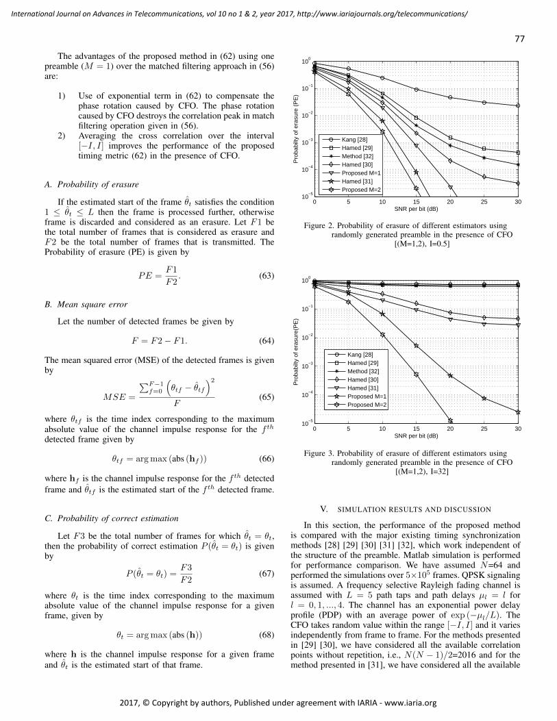
The advantages of the proposed method in (62) using onepreamble (M = 1) over the matched filtering approach in (56)are:

1) Use of exponential term in (62) to compensate thephase rotation caused by CFO. The phase rotationcaused by CFO destroys the correlation peak in matchfiltering operation given in (56).

2) Averaging the cross correlation over the interval[−I, I] improves the performance of the proposedtiming metric (62) in the presence of CFO.

A. Probability of erasure

If the estimated start of the frame θt satisfies the condition1 ≤ θt ≤ L then the frame is processed further, otherwiseframe is discarded and considered as an erasure. Let F1 bethe total number of frames that is considered as erasure andF2 be the total number of frames that is transmitted. TheProbability of erasure (PE) is given by

PE =F1

F2. (63)

B. Mean square error

Let the number of detected frames be given by

F = F2− F1. (64)

The mean squared error (MSE) of the detected frames is givenby

MSE =

∑F−1f=0

(θtf − θtf

)2F

(65)

where θtf is the time index corresponding to the maximumabsolute value of the channel impulse response for the f th

detected frame given by

θtf = argmax (abs (hf )) (66)

where hf is the channel impulse response for the f th detectedframe and θtf is the estimated start of the f th detected frame.

C. Probability of correct estimation

Let F3 be the total number of frames for which θt = θt,then the probability of correct estimation P (θt = θt) is givenby

P (θt = θt) =F3

F2(67)

where θt is the time index corresponding to the maximumabsolute value of the channel impulse response for a givenframe, given by

θt = argmax (abs (h)) (68)

where h is the channel impulse response for a given frameand θt is the estimated start of that frame.

0 5 10 15 20 25 3010

−5

10−4

10−3

10−2

10−1

100

SNR per bit (dB)

Pro

babi

lty o

f era

sure

(P

E)

Kang [28]Hamed [29]Method [32]Hamed [30]Proposed M=1Hamed [31]Proposed M=2

Figure 2. Probability of erasure of different estimators usingrandomly generated preamble in the presence of CFO

[(M=1,2), I=0.5]

0 5 10 15 20 25 3010

−5

10−4

10−3

10−2

10−1

100

SNR per bit (dB)

Pro

babi

lty o

f era

sure

(PE

)

Kang [28]Hamed [29]Method [32]Hamed [30]Hamed [31]Proposed M=1Proposed M=2

Figure 3. Probability of erasure of different estimators usingrandomly generated preamble in the presence of CFO

[(M=1,2), I=32]

V. SIMULATION RESULTS AND DISCUSSION

In this section, the performance of the proposed methodis compared with the major existing timing synchronizationmethods [28] [29] [30] [31] [32], which work independent ofthe structure of the preamble. Matlab simulation is performedfor performance comparison. We have assumed N=64 andperformed the simulations over 5×105 frames. QPSK signalingis assumed. A frequency selective Rayleigh fading channel isassumed with L = 5 path taps and path delays µl = l forl = 0, 1, ..., 4. The channel has an exponential power delayprofile (PDP) with an average power of exp (−µl/L). TheCFO takes random value within the range [−I, I] and it variesindependently from frame to frame. For the methods presentedin [29] [30], we have considered all the available correlationpoints without repetition, i.e., N(N − 1)/2=2016 and for themethod presented in [31], we have considered all the available

77



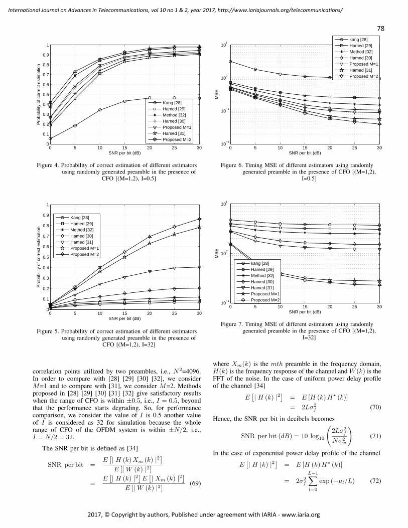
0 5 10 15 20 25 300

0.1

0.2

0.3

0.4

0.5

0.6

0.7

0.8

0.9

1

SNR per bit (dB)

Pro

babi

lity

of c

orre

ct e

stim

atio

n

Kang [28]Hamed [29]Method [32]Hamed [30]Proposed M=1Hamed [31]Proposed M=2

Figure 4. Probability of correct estimation of different estimatorsusing randomly generated preamble in the presence of

CFO [(M=1,2), I=0.5]

0 5 10 15 20 25 300

0.1

0.2

0.3

0.4

0.5

0.6

0.7

0.8

0.9

1

SNR per bit (dB)

Pro

babi

lity

of c

orre

ct e

stim

atio

n

Kang [28]Hamed [29]Method [32]Hamed [30]Hamed [31]Proposed M=1Proposed M=2

Figure 5. Probability of correct estimation of different estimatorsusing randomly generated preamble in the presence of

CFO [(M=1,2), I=32]

correlation points utilized by two preambles, i.e., N2=4096.In order to compare with [28] [29] [30] [32], we considerM=1 and to compare with [31], we consider M=2. Methodsproposed in [28] [29] [30] [31] [32] give satisfactory resultswhen the range of CFO is within ±0.5, i.e., I = 0.5, beyondthat the performance starts degrading. So, for performancecomparison, we consider the value of I is 0.5 another valueof I is considered as 32 for simulation because the wholerange of CFO of the OFDM system is within ±N/2, i.e.,I = N/2 = 32.

The SNR per bit is defined as [34]

SNR per bit =E[| H (k)Xm (k) |2

]E [|W (k) |2]

=E[| H (k) |2

]E[| Xm (k) |2

]E [|W (k) |2]

(69)

0 5 10 15 20 25 3010

−2

10−1

100

101

SNR per bit (dB)

MS

E

kang [28]Hamed [29]Method [32]Hamed [30]Proposed M=1Hamed [31]Proposed M=2

Figure 6. Timing MSE of different estimators using randomlygenerated preamble in the presence of CFO [(M=1,2),

I=0.5]

0 5 10 15 20 25 3010

−1

100

101

SNR per bit (dB)

MS

E

kang [28]Hamed [29]Method [32]Hamed [30]Hamed [31]Proposed M=1Proposed M=2

Figure 7. Timing MSE of different estimators using randomlygenerated preamble in the presence of CFO [(M=1,2),

I=32]

where Xm(k) is the mth preamble in the frequency domain,H(k) is the frequency response of the channel and W (k) is theFFT of the noise. In the case of uniform power delay profileof the channel [34]

E[| H (k) |2

]= E [H (k)H? (k)]

= 2Lσ2f (70)

Hence, the SNR per bit in decibels becomes

SNR per bit (dB) = 10 log10

(2Lσ2

f

Nσ2w

)(71)

In the case of exponential power delay profile of the channel

E[| H (k) |2

]= E [H (k)H? (k)]

= 2σ2f

L−1∑l=0

exp (−µl/L) (72)

78



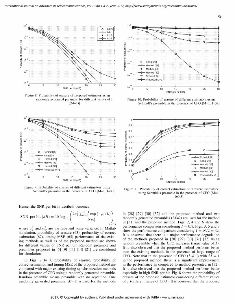
0 5 10 15 20 25 3010

−5

10−4

10−3

10−2

10−1

100

SNR per bit (dB)

Pro

babi

lty o

f era

sure

(P

E)

I=0.5I=8I=16I=32

Figure 8. Probability of erasure of proposed estimator usingrandomly generated preamble for different values of I

[(M=1)]

0 5 10 15 20 25 3010

−5

10−4

10−3

10−2

10−1

100

SNR per bit (dB)

Pro

babi

lty o

f era

sure

(P

E)

Schmidl [5]Kang [28]Hamed [29]Method [32]Hamed [30]Proposed M=1

Figure 9. Probability of erasure of different estimators usingSchmidl’s preamble in the presence of CFO [M=1, I=0.5]

Hence, the SNR per bit in decibels becomes

SNR per bit (dB) = 10 log10

(2σ2

f

∑L−1l=0 exp (−µl/L)Nσ2

w

)(73)

where σ2f and σ2

w are the fade and noise variance. In Matlabsimulation, probability of erasure (63), probability of correctestimation (67), timing MSE (65) performance of the exist-ing methods as well as of the proposed method are shownfor different values of SNR per bit. Random preamble andpreambles proposed in [5] [9] [11] [14] [21] are consideredfor simulation.

In Figs. 2 to 7, probability of erasure, probability ofcorrect estimation and timing MSE of the proposed method arecompared with major existing timing synchronization methodsin the presence of CFO using a randomly generated preamble.Random preamble means preamble with no repetition. Onerandomly generated preamble (M=1) is used for the methods

0 5 10 15 20 25 3010

−5

10−4

10−3

10−2

10−1

100

SNR per bit (dB)

Pro

babi

lty o

f era

sure

(PE

)

Kang [28]Hamed [29]Method [32]Hamed [30]Schmidl [5]Proposed M=1

Figure 10. Probability of erasure of different estimators usingSchmidl’s preamble in the presence of CFO [M=1, I=32]

0 5 10 15 20 25 300

0.1

0.2

0.3

0.4

0.5

0.6

0.7

0.8

0.9

1

SNR per bit (dB)

Pro

babi

lity

of c

orre

ct e

stim

atio

n


Figure 11. Probability of correct estimation of different estimatorsusing Schmidl’s preamble in the presence of CFO [M=1,

I=0.5]

in [28] [29] [30] [32] and the proposed method and tworandomly generated preambles (M=2) are used for the methodin [31] and the proposed method. Figs. 2, 4 and 6 show theperformance comparison considering I = 0.5. Figs. 3, 5 and 7show the performance comparison considering I = N/2 = 32.It is observed that there is a major performance degradationof the methods proposed in [28] [29] [30] [31] [32] usingrandom preamble when the CFO increases (large value of I).It is also observed that the proposed method performs betterthan the existing methods in the presence of large range ofCFO. Note that in the presence of CFO (I 6= 0) with M = 1in the proposed method, there is a significant improvementin the performance as compared to method presented in [32].It is also observed that the proposed method performs betterespecially in high SNR per bit. Fig. 8 shows the probability oferasure of the proposed estimator considering different valuesof I (different range of CFO). It is observed that the proposed

79



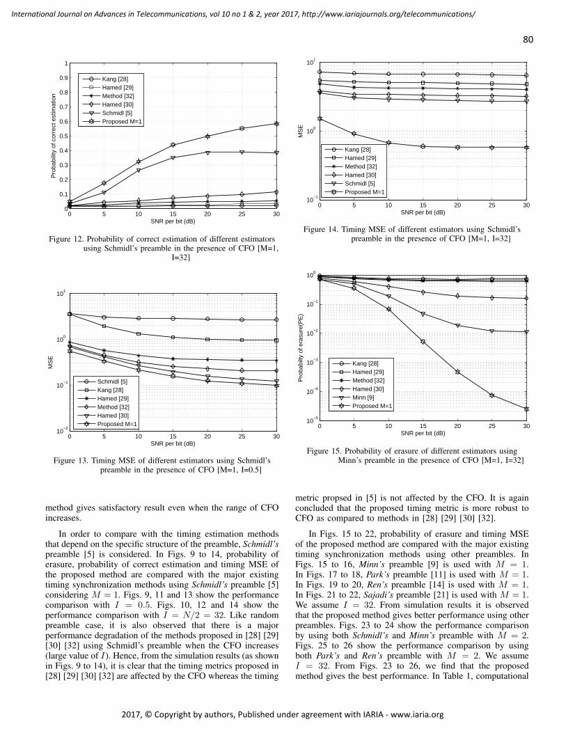
0 5 10 15 20 25 300

0.1

0.2

0.3

0.4

0.5

0.6

0.7

0.8

0.9

1

SNR per bit (dB)

Pro

babi

lity

of c

orre

ct e

stim

atio

n


Figure 12. Probability of correct estimation of different estimatorsusing Schmidl’s preamble in the presence of CFO [M=1,

I=32]

0 5 10 15 20 25 3010

−2

10−1

100

101

SNR per bit (dB)

MS

E


Figure 13. Timing MSE of different estimators using Schmidl’spreamble in the presence of CFO [M=1, I=0.5]

method gives satisfactory result even when the range of CFOincreases.

In order to compare with the timing estimation methodsthat depend on the specific structure of the preamble, Schmidl’spreamble [5] is considered. In Figs. 9 to 14, probability oferasure, probability of correct estimation and timing MSE ofthe proposed method are compared with the major existingtiming synchronization methods using Schmidl’s preamble [5]considering M = 1. Figs. 9, 11 and 13 show the performancecomparison with I = 0.5. Figs. 10, 12 and 14 show theperformance comparison with I = N/2 = 32. Like randompreamble case, it is also observed that there is a majorperformance degradation of the methods proposed in [28] [29][30] [32] using Schmidl’s preamble when the CFO increases(large value of I). Hence, from the simulation results (as shownin Figs. 9 to 14), it is clear that the timing metrics proposed in[28] [29] [30] [32] are affected by the CFO whereas the timing

0 5 10 15 20 25 3010

−1

100

101

SNR per bit (dB)

MS

E


Figure 14. Timing MSE of different estimators using Schmidl’spreamble in the presence of CFO [M=1, I=32]

0 5 10 15 20 25 3010

−5

10−4

10−3

10−2

10−1

100

SNR per bit (dB)

Pro

babi

lty o

f era

sure

(PE

)

Kang [28]Hamed [29]Method [32]Hamed [30]Minn [9]Proposed M=1

Figure 15. Probability of erasure of different estimators usingMinn’s preamble in the presence of CFO [M=1, I=32]

metric propsed in [5] is not affected by the CFO. It is againconcluded that the proposed timing metric is more robust toCFO as compared to methods in [28] [29] [30] [32].

In Figs. 15 to 22, probability of erasure and timing MSEof the proposed method are compared with the major existingtiming synchronization methods using other preambles. InFigs. 15 to 16, Minn’s preamble [9] is used with M = 1.In Figs. 17 to 18, Park’s preamble [11] is used with M = 1.In Figs. 19 to 20, Ren’s preamble [14] is used with M = 1.In Figs. 21 to 22, Sajadi’s preamble [21] is used with M = 1.We assume I = 32. From simulation results it is observedthat the proposed method gives better performance using otherpreambles. Figs. 23 to 24 show the performance comparisonby using both Schmidl’s and Minn’s preamble with M = 2.Figs. 25 to 26 show the performance comparison by usingboth Park’s and Ren’s preamble with M = 2. We assumeI = 32. From Figs. 23 to 26, we find that the proposedmethod gives the best performance. In Table 1, computational

80



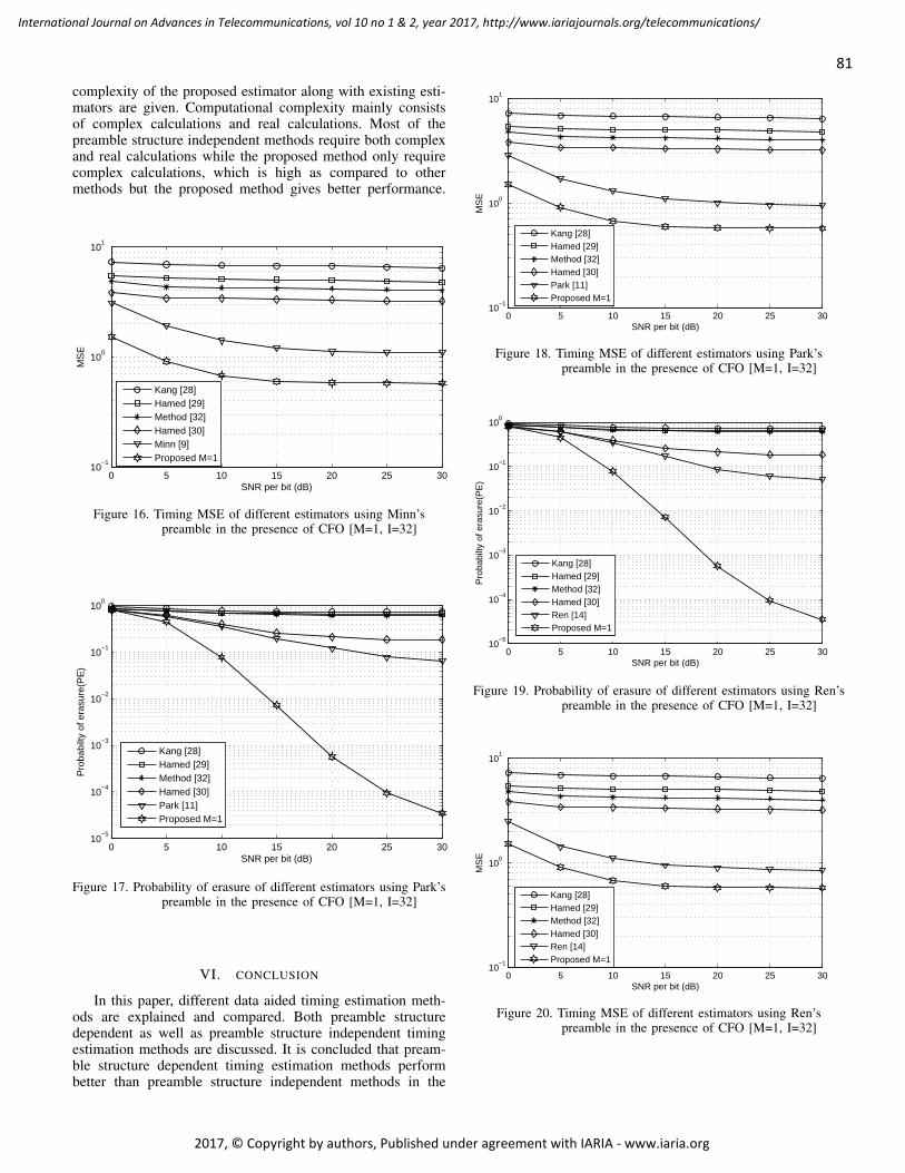
complexity of the proposed estimator along with existing esti-mators are given. Computational complexity mainly consistsof complex calculations and real calculations. Most of thepreamble structure independent methods require both complexand real calculations while the proposed method only requirecomplex calculations, which is high as compared to othermethods but the proposed method gives better performance.

0 5 10 15 20 25 3010

−1

100

101

SNR per bit (dB)

MS

E

Kang [28]Hamed [29]Method [32]Hamed [30]Minn [9]Proposed M=1

Figure 16. Timing MSE of different estimators using Minn’spreamble in the presence of CFO [M=1, I=32]

0 5 10 15 20 25 3010

−5

10−4

10−3

10−2

10−1

100

SNR per bit (dB)

Pro

babi

lty o

f era

sure

(PE

)

Kang [28]Hamed [29]Method [32]Hamed [30]Park [11]Proposed M=1

Figure 17. Probability of erasure of different estimators using Park’spreamble in the presence of CFO [M=1, I=32]

VI. CONCLUSION

In this paper, different data aided timing estimation meth-ods are explained and compared. Both preamble structuredependent as well as preamble structure independent timingestimation methods are discussed. It is concluded that pream-ble structure dependent timing estimation methods performbetter than preamble structure independent methods in the

0 5 10 15 20 25 3010

−1

100

101

SNR per bit (dB)

MS

E

Kang [28]Hamed [29]Method [32]Hamed [30]Park [11]Proposed M=1

Figure 18. Timing MSE of different estimators using Park’spreamble in the presence of CFO [M=1, I=32]

0 5 10 15 20 25 3010

−5

10−4

10−3

10−2

10−1

100

SNR per bit (dB)

Pro

babi

lty o

f era

sure

(PE

)

Kang [28]Hamed [29]Method [32]Hamed [30]Ren [14]Proposed M=1

Figure 19. Probability of erasure of different estimators using Ren’spreamble in the presence of CFO [M=1, I=32]

0 5 10 15 20 25 3010

−1

100

101

SNR per bit (dB)

MS

E

Kang [28]Hamed [29]Method [32]Hamed [30]Ren [14]Proposed M=1

Figure 20. Timing MSE of different estimators using Ren’spreamble in the presence of CFO [M=1, I=32]

81



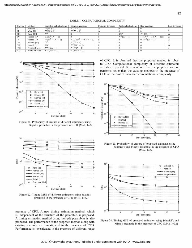
TABLE I: COMPUTATIONAL COMPLEXITY

Sl. No. Method Complex multiplications Complex additions Complex divisions Real multiplications Real additions Real divisionsI Schmidl [5] N(N + 2) N(N − 2) N 0 0 0II Minn [9] N(N + 2) N(N − 2) N 0 0 0III Kang [28] N2 0 0 2N2 N(3N − 1) N

IV Hamed [29] 0.5N2(N − 1) 0 0 N2(N − 1) (1.5N2 − 1.5N − 1)N N

V Hamed [30] N(N2 −N + 1) N(0.5N2 − 0.5N − 1) 0 0 0.5N2(N − 1) N

VI Method [32] N2 N(N − 1) N 0 0 0

VII Hamed [31] 3N3 N(2N2 − 2) 0 0 0 NVIII Proposed M=1 PN(2N + 1) N(NP − 1) 0 0 0 0IX Proposed M=2 PN(4N + 1) N(2NP − 1) 0 0 0 0

0 5 10 15 20 25 3010

−5

10−4

10−3

10−2

10−1

100

SNR per bit (dB)

Pro

babi

lty o

f era

sure

(PE

)

Kang [28]Hamed [29]Method [32]Hamed [30]Sajadi [21]Proposed M=1

Figure 21. Probability of erasure of different estimators usingSajadi’s preamble in the presence of CFO [M=1, I=32]

0 5 10 15 20 25 3010

−1

100

101

SNR per bit (dB)

MS

E

Kang [28]Hamed [29]Method [32]Hamed [30]Sajadi [21]Proposed M=1

Figure 22. Timing MSE of different estimators using Sajadi’spreamble in the presence of CFO [M=1, I=32]

presence of CFO. A new timing estimation method, whichis independent of the structure of the preamble, is proposed.A timing estimation method using multiple preambles is alsoproposed. The performance of the proposed method along withexisting methods are investigated in the presence of CFO.Performance is investigated in the presence of different range

of CFO. It is observed that the proposed method is robustto CFO. Computational complexity of different estimatorsare also explained. It is observed that the proposed methodperforms better than the existing methods in the presence ofCFO at the cost of increased computational complexity.

0 5 10 15 20 25 3010

−5

10−4

10−3

10−2

10−1

100

SNR per bit (dB)

Pro

babi

lty o

f era

sure

(PE

)

Schmidl [5]Minn [9]Hamed [31]Proposed M=2

Figure 23. Probability of erasure of proposed estimator usingSchmidl’s and Minn’s preamble in the presence of CFO

[M=2, I=32]

0 5 10 15 20 25 3010

−1

100

101

SNR per bit (dB)

MS

E

Schmidl [5]Minn [9]Hamed [31]Proposed M=2

Figure 24. Timing MSE of proposed estimator using Schmidl’s andMinn’s preamble in the presence of CFO [M=2, I=32]

82



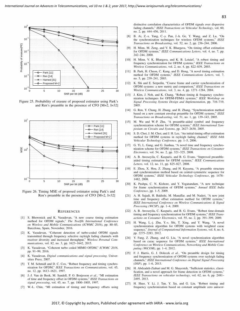
0 5 10 15 20 25 3010

−5

10−4

10−3

10−2

10−1

100

SNR per bit (dB)

Pro

babi

lty o

f era

sure

(PE

)

Park [11]Ren [14]Hamed [31]Proposed M=2

Figure 25. Probability of erasure of proposed estimator using Park’sand Ren’s preamble in the presence of CFO [M=2, I=32]

0 5 10 15 20 25 3010

−1

100

101

SNR per bit (dB)

MS

E

Park [11]Ren [14]Hamed [31]Proposed M=2

Figure 26. Timing MSE of proposed estimator using Park’s andRen’s preamble in the presence of CFO [M=2, I=32]

REFERENCES

[1] S. Bhowmick and K. Vasudevan, “A new coarse timing estimationmethod for OFDM signals,” The Twelfth International Conferenceon Wireless and Mobile Communications (ICWMC 2016), pp. 80–85,Barcelona, Spain, November, 2016.

[2] K. Vasudevan, “Coherent detection of turbo-coded OFDM signalstransmitted through frequency selective rayleigh fading channels withreceiver diversity and increased throughput,” Wireless Personal Com-munications, vol. 82, no. 3, pp. 1623–1642, 2015.

[3] K. Vasudevan, “Coherent turbo coded MIMO OFDM,” ICWMC 2016,pp. 91–99, 2016.

[4] K. Vasudevan, Digital communications and signal processing. Univer-sities Press, 2007.

[5] T. M. Schmidl and D. C. Cox, “Robust frequency and timing synchro-nization for OFDM,” IEEE Transactions on Communications, vol. 45,no. 12, pp. 1613–1621, 1997.

[6] J.-J. Van de Beek, M. Sandell, P. O. Borjesson et al., “Ml estimationof time and frequency offset in OFDM systems,” IEEE Transactions onsignal processing, vol. 45, no. 7, pp. 1800–1805, 1997.

[7] W.-L. Chin, “Ml estimation of timing and frequency offsets using

distinctive correlation characteristics of OFDM signals over dispersivefading channels,” IEEE Transactions on Vehicular Technology, vol. 60,no. 2, pp. 444–456, 2011.

[8] B. Ai, Z.-x. Yang, C.-y. Pan, J.-h. Ge, Y. Wang, and Z. Lu, “Onthe synchronization techniques for wireless OFDM systems,” IEEETransactions on Broadcasting, vol. 52, no. 2, pp. 236–244, 2006.

[9] H. Minn, M. Zeng, and V. K. Bhargava, “On timing offset estimationfor OFDM systems,” IEEE Communications Letters, vol. 4, no. 7, pp.242–244, 2000.

[10] H. Minn, V. K. Bhargava, and K. B. Letaief, “A robust timing andfrequency synchronization for OFDM systems,” IEEE Transactions onWireless Communications, vol. 2, no. 4, pp. 822–839, 2003.

[11] B. Park, H. Cheon, C. Kang, and D. Hong, “A novel timing estimationmethod for OFDM systems,” IEEE Communications Letters, vol. 7,no. 5, pp. 239–241, 2003.

[12] K. Shi and E. Serpedin, “Coarse frame and carrier synchronization ofOFDM systems: a new metric and comparison,” IEEE Transactions onWireless Communications, vol. 3, no. 4, pp. 1271–1284, 2004.

[13] J. Kim, J. Noh, and K. Chang, “Robust timing & frequency synchro-nization techniques for OFDM-FDMA systems,” IEEE Workshop onSignal Processing Systems Design and Implementation, pp. 716–719,2005.

[14] G. Ren, Y. Chang, H. Zhang, and H. Zhang, “Synchronization methodbased on a new constant envelop preamble for OFDM systems,” IEEETransactions on Broadcasting, vol. 51, no. 1, pp. 139–143, 2005.

[15] M. Wu and W.-P. Zhu, “A preamble-aided symbol and frequencysynchronization scheme for OFDM systems,” IEEE International Sym-posium on Circuits and Systems, pp. 2627–2630, 2005.

[16] S. D. Choi, J. M. Choi, and J. H. Lee, “An initial timing offset estimationmethod for OFDM systems in rayleigh fading channel,” IEEE 64thVehicular Technology Conference, pp. 1–5, 2006.

[17] G. Yi, L. Gang, and G. Jianhua, “A novel time and frequency synchro-nization scheme for OFDM systems,” IEEE Transactions on ConsumerElectronics, vol. 54, no. 2, pp. 321–325, 2008.

[18] A. B. Awoseyila, C. Kasparis, and B. G. Evans, “Improved preamble-aided timing estimation for OFDM systems,” IEEE CommunicationsLetters, vol. 12, no. 11, pp. 825–827, 2008.

[19] E. Zhou, X. Hou, Z. Zhang, and H. Kayama, “A preamble structureand synchronization method based on central-symmetric sequence forOFDM systems,” IEEE Vehicular Technology Conference, pp. 1478–1482, 2008.

[20] K. Pushpa, C. N. Kishore, and Y. Yoganandam, “A new techniquefor frame synchronization of OFDM systems,” Annual IEEE IndiaConference, pp. 1–5, 2009.

[21] A. H. Sajadi, H. Bakhshi, M. Manaffar, and M. Naderi, “A new jointtime and frequency offset estimation method for OFDM systems,”IEEE International Conference on Wireless Communications & SignalProcessing (WCSP), pp. 1–4, 2009.

[22] A. B. Awoseyila, C. Kasparis, and B. G. Evans, “Robust time-domaintiming and frequency synchronization for OFDM systems,” IEEE Trans-actions on Consumer Electronics, vol. 55, no. 2, pp. 391–399, 2009.

[23] H. Wang, L.-j. Zhu, Y.-s. Shi, T. Xing, and Y. Wang, “A novelsynchronization algorithm for OFDM systems with weighted cazacsequence,” Journal of Computational Information Systems, vol. 8, no. 6,pp. 2275–2283, 2012.

[24] Y. Fang, Z. Zhang, and G. Liu, “A novel synchronization algorithmbased on cazac sequence for OFDM systems,” IEEE InternationalConference on Wireless Communications, Networking and Mobile Com-puting (WiCOM), pp. 1–4, 2012.

[25] F. J. Harris, G. J. Dolecek et al., “On preamble design for timingand frequency synchronization of OFDM systems over rayleigh fadingchannels,” IEEE International Conference on Digital Signal Processing(DSP), pp. 1–6, 2013.

[26] H. Abdzadeh-Ziabari and M. G. Shayesteh, “Sufficient statistics, classi-fication, and a novel approach for frame detection in OFDM systems,”IEEE Transactions on vehicular technology, vol. 62, no. 6, pp. 2481–2495, 2013.

[27] H. Shao, Y. Li, J. Tan, Y. Xu, and G. Liu, “Robust timing andfrequency synchronization based on constant amplitude zero autocor-

83



relation sequence for OFDM systems,” IEEE International Conferenceon Communication Problem-Solving (ICCP), pp. 14–17, 2014.

[28] Y. Kang, S. Kim, D. Ahn, and H. Lee, “Timing estimation for OFDMsystems by using a correlation sequence of preamble,” IEEE Transac-tions on Consumer Electronics, vol. 54, no. 4, pp. 1600–1608, 2008.

[29] H. Abdzadeh-Ziabari, M. G. Shayesteh, and M. Manaffar, “An improvedtiming estimation method for OFDM systems,” IEEE Transactions onConsumer Electronics, vol. 56, no. 4, pp. 2098–2105, 2010.

[30] H. Abdzadeh-Ziabari and M. G. Shayesteh, “Robust timing and fre-quency synchronization for OFDM systems,” IEEE Transactions onVehicular Technology, vol. 60, no. 8, pp. 3646–3656, 2011.

[31] H. Abdzadeh-Ziabari and M. G. Shayesteh, “A novel preamble-basedframe timing estimator for OFDM systems,” IEEE CommunicationsLetters, vol. 16, no. 7, pp. 1121–1124, 2012.

[32] U. Samal and K. Vasudevan, “Preamble-based timing synchronizationfor OFDM systems,” IEEE 3rd International Advance ComputingConference (IACC), pp. 313–318, 2013.

[33] A. Saadat, M. Salman, and H. Saadat, “Matched filter based timingsynchronization for orthogonal frequency division multiplexing sys-tems,” IEEE 8th Conference on Industrial Electronics and Applications(ICIEA), pp. 1156–1161, 2013.

[34] K. Vasudevan, “Coherent detection of turbo coded OFDM signalstransmitted through frequency selective rayleigh fading channels,” IEEEInternational Conference on Signal Processing, Computing and Control(ISPCC), pp. 1–6, 2013.

84



www.iariajournals.org

International Journal On Advances in Intelligent Systems

issn: 1942-2679

International Journal On Advances in Internet Technology

issn: 1942-2652

International Journal On Advances in Life Sciences

issn: 1942-2660

International Journal On Advances in Networks and Services

issn: 1942-2644

International Journal On Advances in Security

issn: 1942-2636

International Journal On Advances in Software

issn: 1942-2628

International Journal On Advances in Systems and Measurements

issn: 1942-261x

International Journal On Advances in Telecommunications

issn: 1942-2601

the - iaria journals · antónio manuel duarte nogueira, ... canada / liverpool john moores...

Documents