the effects of volatility misestimation on option-replication portfolio insurance

CFA Institute

The Effects of Volatility Misestimation on Option-Replication Portfolio InsuranceAuthor(s): Richard J. Rendleman, Jr. and Thomas J. O'BrienSource: Financial Analysts Journal, Vol. 46, No. 3 (May - Jun., 1990), pp. 61-70Published by: CFA InstituteStable URL: http://www.jstor.org/stable/4479331 .

Accessed: 17/06/2014 12:58

Your use of the JSTOR archive indicates your acceptance of the Terms & Conditions of Use, available at .http://www.jstor.org/page/info/about/policies/terms.jsp

.JSTOR is a not-for-profit service that helps scholars, researchers, and students discover, use, and build upon a wide range ofcontent in a trusted digital archive. We use information technology and tools to increase productivity and facilitate new formsof scholarship. For more information about JSTOR, please contact [email protected].

.

CFA Institute is collaborating with JSTOR to digitize, preserve and extend access to Financial AnalystsJournal.

http://www.jstor.org

This content downloaded from 185.44.79.85 on Tue, 17 Jun 2014 12:58:49 PMAll use subject to JSTOR Terms and Conditions

http://www.jstor.org/action/showPublisher?publisherCode=cfa

http://www.jstor.org/stable/4479331?origin=JSTOR-pdf

http://www.jstor.org/page/info/about/policies/terms.jsp


by Richard J. Rendleman, Jr. and Thomas J. O'Brien

The Effects of Volatility Misestimation on Option-Replication

Portfolio Insurance

To insure a stock portfolio, one could purchase a put option with a striking price equal to some desired minimum value for the portfolio. Alternatively, one could replicate this stock-plus-put portfolio with a portfolio of stock and cash. The initial allocations to stock and cash will depend upon the parameters of an option valuation formula and will change as those parameters change. In particular, the construction of such synthetic, option- replicating portfolio insurance, hence its outcome, will depend critically on correct estimation of the volatility of the portfolio being insured.

Volatility misestimation will cause the price of the synthetic put to deviate from its expected price and will result in incorrect allocations between stock and cash. As a result, the outcome of a synthetic portfolio insurance strategy based on misestimated volatility will be unpredictable. A manager who underestimates volatility will typically end up buying less insurance than is necessary to ensure a given return, while a manager who overestimates volatility will buy more insurance than is necessary. Both outcomes can be costly in terms of missed floors and forgone gains.

Simulations of portfolio insurance performance over the period of the October 1987 market crash indicate that most insured portfolios would have fallen short of their promised values. In general, however, the lower the guaranteed floor of the insurance program (hence the lower its insurance), the worse its results.

T HE MOST STRAIGHTFORWARD method of insuring a given return to a portfolio of risky assets is to purchase put

options on the portfolio. Alternatively, a dynamic portfolio of stock and cash can be created to replicate the effects of the put options.1 Such

synthetic, option-replicating strategies for portfolio insurance can be expected to perform well-if the volatility of the portfolio being insured is estimated accurately. Misestimation of this volatility can cause the outcome of a synthetic portfolio insurance strategy to deviate significantly from its target.

This article analyzes three effects associated with volatility misestimation in synthetic portfolio insurance programs. The first effect is mispricing: Differences between expected and realized volatility will cause the effective price of a synthetic put to deviate from its expected price. The second effect is misallocation of portfolio insurance funds: When a portfolio manager estimates volatility incorrectly, he or she will end up purchasing the wrong synthetic put

1. Footnotes appear at end of article.

Richard Rendleman, Jr. is Professor of Finance at the University of North Carolina Business School at Chapel Hill. Thomas O'Brien is Associate Professor of Finance at the University of Connecticut School of Business.

The authors thank Phillip Davis for his research assis- tance and Jennifer Conrad, Ted Day, Dwight Grant, Bruce Jacobs and Richard McEnally for their helpful comments. An earlier version of this article was presented at the 1988 meeting of the Southern Economic Association.

FINANCIAL ANALYSTS JOURNAL / MAY-JUNE 1990 a 61



option, misallocating assets between stock and cash. The third effect is uncertainty: The outcome of a synthetic insurance program that misestimates volatility will be unpredictable.

Background Asay and Edelsberg examined the problem of volatility misestimation in the context of synthetic portfolio insurance but dismissed it as insignificant.2 Their conclusions, however, appear to be based on an examination of insured portfolios of Treasury-bill futures, which have relatively low volatilities in comparison to stock and other financial assets. Hill, Jain and Wood studied the volatility misestimation problem as it pertains to stocks and found that misestimation is a serious problem.3 However, they only addressed the mispricing effect, and their analysis of that effect was limited.

The results of two other studies suggest that synthetically insured portfolios may perform poorly when volatility is misestimated. Garcia and Gould examined simulated synthetic portfolio insurance strategies using historical data from the 1963-83 period. While not specifically addressing the volatility misestimation problem, they found that "no matter what volatility estimate was used, [their option-replicating procedure] produced unsatisfactory results in the sense that the downside floor could not be tightly controlled."4 Figlewski studied the effect of volatility misestimation on synthetic risk-free hedges and found a significant impact.5 He did not, however, address directly the problem of volatility misestimation as it relates to synthetic portfolio insurance.

The Theory of Portfolio Insurance In principle, insuring a portfolio of risky as-

sets involves nothing more than purchasing a put option with a striking price equal to some desired minimum value for the portfolio. Con- sider, for example, an insurance program for a stock portfolio that was originally worth $100 and that is insured for $100 at the end of one year. Assume the riskless interest rate is 7 per cent compounded annually (or 6.766 per cent compounded continuously) and the logarithmic volatility (standard deviation) of the stock portfolio is 20 per cent per year. The stock pays no dividends (or equivalently, any dividends are immediately reinvested in the stock).6

We assume that the Black-Scholes option- pricing model is appropriate for determining the

value of the put option.7 The Black-Scholes valuation equation for put options is expressed as follows:

P = S * (N(dl) - 1) + K * EXP( - rt)

(1 - N(d2))%1

dl = [ln(S/K) + (r + 0.5v2)t] / [vt0 5] and

d2 = dl - vt0o5,

where

P = the value of the put, S = the value of the underlying stock (or

stock portfolio), K = the put's striking price, v = the annual logarithmic volatility (stan-

dard deviation) of the underlying stocks' returns,

r = the annual, continuously compounded riskless rate of interest and

t = the number of years until the option's maturity date.

EXP( ) denotes exponentiation, and N( ) represents the unit normal distribution function. One can add the value of the stock, S, to both sides of Equation (1) to obtain the value of the stock plus a put (i.e., an insured stock):

S + P = S * N(dl) +K K EXP( - rt)

(1 - N(d2)). (2)

The cost of insuring a $100 portfolio for a $100 end-of-period value can be found by solving for the dollar value of the stock, S, such that S + P in Equation (2) equals $100, where P is the value of a put option with a striking price of $100 on a stock with a value of S. Through trial and error, we arrive at values for S and P of, respectively, $91.73 and $8.27. Thus, with $100 of original capital, one could purchase one "unit," or share, of stock at a price of $91.73 per share and one put with a $100 striking price on this same share for a price of $8.27.

Equation (2) also provides the key to creating a synthetic portfolio insurance program. Accord- ing to Equation (2), if we want to replicate a portfolio containing the stock plus the put, we must hold N(dl) shares of the stock and invest an amount equal to K * EXP(-rt) (1 - N(d2)) in a riskless asset. And, as changes in S and t change N(dl) and N(d2), we must be prepared to trade between the stock and the riskless asset

FINANCIAL ANALYSTS JOURNAL / MAY-JUNE 1990 O 62



Figure A Mispricing and Misallocation in Synthetic Portfolio Insurance

200 Low Expectation

180 -

160 -

z 140 -

? 120 H igh Expectation

C?100 .M

C 80

E 60 -

40 -

20 -~

'I~~~J 20 , I* ;.E. I * _ l ii * I * I .i l i

0 20 40 60 80 100 120 140 160 180 200 Stock Price Per Share ($)

so as to maintain the proper portfolio mix. This is the essence of synthetic insurance.

For our example, N(dl) equals 0.5026. There- fore, our specific synthetic insurance program should start out with 0.5026 share of stock at a price of $91.73 per share, for a total stock investment of $46.10 (= 0.5026 $91.73). The rest of the $100-$53.90-should be invested in T-bills. This amount could also be arrived at by solving for the second component of Equation (2); in our example, $100 . EXP (-0.06766) (1 - 0.4233) = $53.90.

As long as the volatility parameter is known with certainty, and portfolio adjustments are made on a continuous basis, this dynamic plan will provide the same horizon profits as a portfolio insured through the direct purchase of a put option. Thus, with known volatility, the eco- nomics of portfolio insurance are the same whether one purchases the protective put directly or through a synthetic option-replication plan with continuous trading.

The Effects of Volatility Misestimation The mispricing and misallocation effects of volatility misestimation can be illustrated by an example that involves the direct purchase of put options, rather than the use of synthetic puts.

Consider two CBOE-type option markets, which trade European puts for use in connection with portfolio insurance programs. The first market-the "high-expectation" market- trades put options at prices that reflect the expectation that the annualized volatility of the index will be 20 per cent. The second market- the "low-expectation" market-trades options at prices that reflect the expectation of 10 per cent volatility.

Both markets use a special settlement procedure at maturity. In settling up, the buyer must pay the difference (plus interest) between the option's original purchase price and the price that would have been paid had the volatility that actually occurred over the option's life been known in advance. If this difference turns out to be negative, the investor will receive a refund. As our simulation results will later show, the price of a synthetic put is determined on an ex post basis in much the same way.8

The Misallocation Effect Consider our earlier example, which involves

the use of portfolio insurance to guarantee a $100 floor in one year for every $100 of initial

capital. A portfolio manager who believes that volatility will be 20 per cent will allocate $91.73 to stock and invest $8.27 in a one-year high- expectation put option with a $100 striking price. For convenience, we will assume that $91.73 represents the price of one share of stock or one unit of a market index.

Figure A plots the end-of-year values of insured portfolios conditional on the end-of-year values of one share of stock. The solid line marked "high expectation" represents the conditional payoff structure that a portfolio manager who uses a 20 per cent volatility estimate will expect when the option matures in one year.9

Now consider a second portfolio manager, who believes the volatility will be 10 per cent. He buys portfolio insurance puts in the low- expectation market, investing $98.05 in stock and $1.95 in a put with a $100 striking price.

Assume that volatility over the year turns out to be 10 per cent. The second manager will have made the proper allocation between stock and puts. In contrast, the high-estimate manager, who believed that volatility would be 20 per cent and employed a $91.73/$8.27 stock/put allocation, will have invested too much in puts and too little in stocks.

The solid line in Figure A marked "low expectation" shows the payoff structure that the low- estimate manager will expect, conditional on the




end-of-year value of one share of stock originally worth $91.73. The manager allocated $98.05 to stock, hence purchased 1.069 (98.05/ 91.73) shares; the slope of the low-expectation line is thus 1.069.

As Figure A indicates, the low-estimate manager can expect to perform better on the upside than the high-estimate manager. There is a small portion of the graph, between end-of-year share prices of $93.55 (100/98.05 . 91.73) and $100, where the low-estimate manager will expect a payoff slightly greater than the $100 guaranteed floor, while the high-estimate manager will still expect a $100 payoff. At stock prices below $93.55, both managers will expect a $100 payoff.

The Mispricing Effect If it were not for the settlement provisions at

maturity, which cause the prices of all option contracts to reflect the ex post volatility, the payoffs available in the low-expectation market would dominate those available in the high- expectation market. With the given settlement procedure, neither market will dominate, but the final portfolio payoffs will differ between the two markets, because investors in the two markets employ different initial allocations between options and stock.

When the ex post volatility turns out to be 10 per cent, no settlement occurs in the low- expectation market; options in that market were initially priced for 10 per cent volatility. How- ever, an adjustment must be made in the high- expectation market, because its initial option premium turns out to have been too high.

In retrospect, investors in the high-expectation market should have paid only $4.62 for the put option they originally purchased for $8.27. 10 At settlement, investors in the high-expectation market will get a refund equal to the difference between the option price actually paid and the price that should have been paid, or $3.65 (8.27 - 4.62), plus interest at 7 per cent, for a total refund of $3.91. This $3.91 refund represents the mispricing effect; its value is independent of the ending portfolio value.

In Figure A, the combined effect of misallocation and mispricing is reflected by the dotted line that parallels the original graph of high- estimate outcomes. This line lies exactly $3.91 above the original payoff line for the high- estimate manager. The mispricing effect, then, causes the guaranteed payoff and all other pay-

offs to be $3.91 higher than expected. The misallocation effect, however, causes a significant opportunity loss in a strong market, because it will result in too low an allocation to stock.

Generalizing from this example, we can con- clude that when volatility is overestimated, the high-estimate investor will suffer a significant opportunity cost in a strong market, but will gain in a moderately flat or down market. This relationship is reversed when volatility is under- estimated.

The Uncertainty Effect As the analysis above suggests, the mispric-

ing and misallocation effects are not unique to synthetic insurance and can occur in direct purchase markets. The uncertainty effect, by contrast, is unique to synthetic options.

The uncertainty effect arises in synthetic insurance because misestimation of volatility will result in an incorrect mix of stock and T-bills throughout the life of the insurance program. This can be seen easily by examining the N(dl) term in Equation (2). This term defines the number of shares of stock required to create a synthetic put. But this term is, itself, a function of the volatility. If the estimated volatility is wrong, the number of shares purchased will be wrong, both initially and throughout the life of the program.

The ending value of a synthetically insured portfolio depends on the price path taken over the term of the insurance program. Because the path cannot be predicted, there will be uncertainty in the outcome. We must resort to simulation to study this effect.

Portfolio Simulations We simulated one-year synthetic insurance programs, making the initial portfolio allocations in the manner described above and employing similar assumptions-$100 of initial capital and an annually compounded risk-free rate of 7 per cent. We assumed each insurance program was implemented as if the portfolio manager believed the volatility of the underlying portfolio was 20 per cent, but the portfolio's true volatility could be different.

Portfolio revisions were made at the end of predetermined time intervals. At the end of each interval, a random stock return was generated from a lognormal distribution with an expected annual logarithmic rate of return of 15 per cent and a standard deviation determined

FINANCIAL ANALYSTS JOURNAL I MAY-JUNE 1990 O 64



Table I The Effect of Noncontinuous Trading on Portfolio Insurance Outcomes (based on 1,000 simulations for each trading period)

Trades per Year

6 12 52 252

Mean Difference -0.060 -0.045 -0.014 0.007 Max. Difference 7.482 6.023 2.700 1.683 Min. Difference -10.509 -9.039 -4.044 -1.601 Std. Deviation 2.729 1.981 0.887 0.429

by the type of experiment under considera- tion. 11

With each randomly generated stock return, a new allocation between stock and T-bills was determined using Equation (2).12 This process of generating a new random stock return and rebalancing to maintain the put replication portfolio weights was repeated until the end of the one-year insurance horizon was reached. One thousand separate simulations were run for each of a large number of scenarios involving both insurance terms and expected volatilities.

Discrete Revision Effect In both the real world and in the world of

simulation, some decision about the timing of portfolio revisions must be made. Revisions can be set by time intervals-for example, daily, weekly or monthly revisions. Alternatively, revisions can be built around changes in the value of the stock portfolio itself, or changes in the number of shares that should be held. We used time-based revisions. Before assessing the costs associated with misestimating volatility, we must assess the possible effects of our choice of revision period.13

In an effort to gauge the extent to which noncontinuous portfolio revisions affect ending portfolio values, we examined strategies that rebalanced N times per year, where N took on values of 6, 12, 52 and 252 (corresponding to semiannual, monthly, weekly and daily rebalancing). The guaranteed insurance floor was assumed to be $100. Table I reports summary figures for the differences between 1,000 simulated horizon insurance values and corresponding horizon values under continuous revision.

All the mean differences between the simulated end-of-year portfolio values and their corresponding theoretical values are close to zero. This is not surprising; the average error should be zero in the absence of bias. What is critical, however, is the amount of deviation in the

outcomes. With weekly rebalancing, for example, one out of 1,000 simulated observations exceeded its theoretical value by $2.70, while another fell short by $4.04. The standard deviation of these differences is $0.887. Weekly rebalancing produced an amount of error that would appear to be within limits most portfolio managers could tolerate. Based on these results, for all subsequent simulations we used weekly revisions.

Simulation Results We assumed that the portfolio manager ex-

pects the volatility of stock returns to be 20 per cent, but that actual volatility turns out to be different. We made no attempt to adapt the insurance program to new information about the realized volatility. We assumed a 7 per cent interest rate and 15 per cent expected stock return throughout.

Table II summarizes the effects of mispricing and uncertainty when volatility is misestimated in connection with synthetic portfolio insurance plans with guaranteed floors of $95, $100 and $105 for every $100 of initial capital.

Consider the $100 insurance floor. In the "expected difference" section of the table, the second row shows the difference between the insurance cost for a plan with a $100 floor based on 20 per cent volatility if the insurance is paid for at the horizon and the amount that should have been paid for the same option if the ex post volatility had been known in advance. For example, the difference of $3.905 in the 10 per cent column is computed as (8.27 - 4.62) * 1.07, where $8.27 is the put price under a 20 per cent volatility assumption and $4.62 is the cost of the same put under a 10 per cent assumption. Except for differences in rounding, this difference corresponds to the settlement cost dis- cussed earlier.

The "mean differences" throughout the table represent the average difference between simulated ending portfolio values and the values that a portfolio manager would expect to occur, conditional on the ending value of the underlying stock portfolio. The "standard deviations" are the standard deviations of this difference. The following example provides an illustration of the difference between the ending portfolio value and its conditional expected value.

Under a 20 per cent volatility assumption, it should cost $8.27 to purchase a put for a $100 insurance program with a $100 floor, leaving

FINANCIAL ANALYSTS JOURNAL / MAY-JUNE 1990 65



Table II Simulated Portfolio Outcomes vs. Expected Outcomes

Actual Volatility (%)

10 12 14 16 18 20 22 24 26 28 30

Expected Differences* Floor = $95 3.430 3.803 2.136 1.439 0.727 0.000 -0.735 -1.478 -2.225 -2.976 -3.739 Floor = $100 3.905 3.129 2.347 1.565 0.783 0.000 -0.783 -1.567 -2.349 -3.130 -3.910 Floor = $105 1.848 1.684 1.329 0.945 0.498 0.000 -0.537 -1.106 -1.700 -2.315 -2.947

All Observationst Floor = $95

Mean Difference 2.800 2.361 1.840 1.308 0.607 0.000 -0.645 -1.463 -2.090 -2.842 -3.552 Std. Deviation 1.340 1.196 1.048 0.883 0.812 0.864 0.990 1.326 1.631 2.048 2.404

Floor = $100 Mean Difference 3.911 3.125 2.343 1.601 0.742 -0.014 -0.754 -1.671 -2.323 -3.117 -4.034 Std. Deviation 1.145 1.055 0.962 0.945 0.859 0.887 1.116 1.379 1.553 1.876 2.349

Floor = $105 Mean Difference 2.563 2.167 1.715 1.140 0.607 0.031 -0.590 -1.310 -1.884 -2.567 -3.225 Std. Deviation 1.340 1.196 1.048 0.883 0.812 0.864 0.990 1.326 1.631 2.048 2.404

Theoretical Value = Floor Floor = $95

Mean Difference 4.275 3.432 2.553 1.718 0.846 0.087 -0.783 -1.692 -2.405 -3.221 -4.055 Std. Deviation 0.820 0.936 0.840 0.847 0.973 0.901 1.075 1.234 1.573 1.734 2.169 # Observations 79 126 141 202 225 259 301 318 332 344 350

Floor = $100 Mean Difference 4.146 3.268 2.482 1.619 0.754 0.018 -0.694 -1.619 -2.219 -2.910 -3.818 Std. Deviation 1.145 1.092 0.954 0.929 0.844 0.897 1.079 1.426 1.654 1.827 2.439 # Observations 308 336 354 409 389 435 437 464 465 461 453

Floor = $105 Mean Difference 2.294 1.916 1.473 0.986 0.544 0.065 -0.478 -1.025 -1.511 -2.038 -2.530 Std. Deviation 1.213 1.097 0.935 0.798 0.711 0.736 0.913 1.155 1.447 1.851 2.154 # Observations 855 831 785 772 731 728 742 716 714 685 679

Theoretical Value > Floor Floor = $95

Mean Difference 2.673 2.207 1.723 1.204 0.538 -0.030 -0.586 -1.357 -1.934 -2.644 -3.281 Std. Deviation 1.038 0.977 0.899 0.809 0.687 0.720 0.953 1.181 1.441 1.802 2.128



I The expected difference is computed by first taking the difference between the value of the portfolio insurance put option evaluated with the actual volatility and the value of the same put evaluated with the expected volatility. This difference is then multiplied by one plus the riskless rate of interest (1.07). t The mean difference is the average value of each simulated portfolio outcome less the corresponding value of its expected outcome, given the ending value of the underlying stock portfolio. The standard deviation is the standard deviation of this difference.

$91.73 to be invested in stock. If the stock were to rise in value by a factor of, say, 1.5 by the end of the insurance horizon, the expected ending value of the insured portfolio would be $137.60 (91.73 * 1.5). Thus, if the portfolio manager thought he was paying $8.27 for the put he would expect the insured portfolio to be worth $137.60 if the stocks in the portfolio increased in value by 50 per cent. If the actual value of the portfolio turned out to be only $135, the manager's performance would fall $2.60 short of expectations. In this case, the cost of "settling up" would be $2.60.

For the portfolios with $100 floors, there is a strikingly close correspondence between the mean and expected differences in ending port-

folio values. It appears that the average difference between the ending value of a portfolio insured synthetically and its expected ending value conditional on the performance of the underlying stock is approximately equal to the difference (plus interest) between the theoretical value of the put evaluated with the expected volatility and the same put evaluated with the realized volatility. Thus, except for the uncertainty in the outcome, the cost of mispricing this "at-the-money" insurance contract (where the initial investment and the guaranteed floor are equal) is essentially the same as the cost that would occur in a direct put purchase plan with the settlement provisions described above.

When the floor of the insurance program does

FINANCIAL ANALYSTS JOURNAL / MAY-JUNE 1990 i3 66



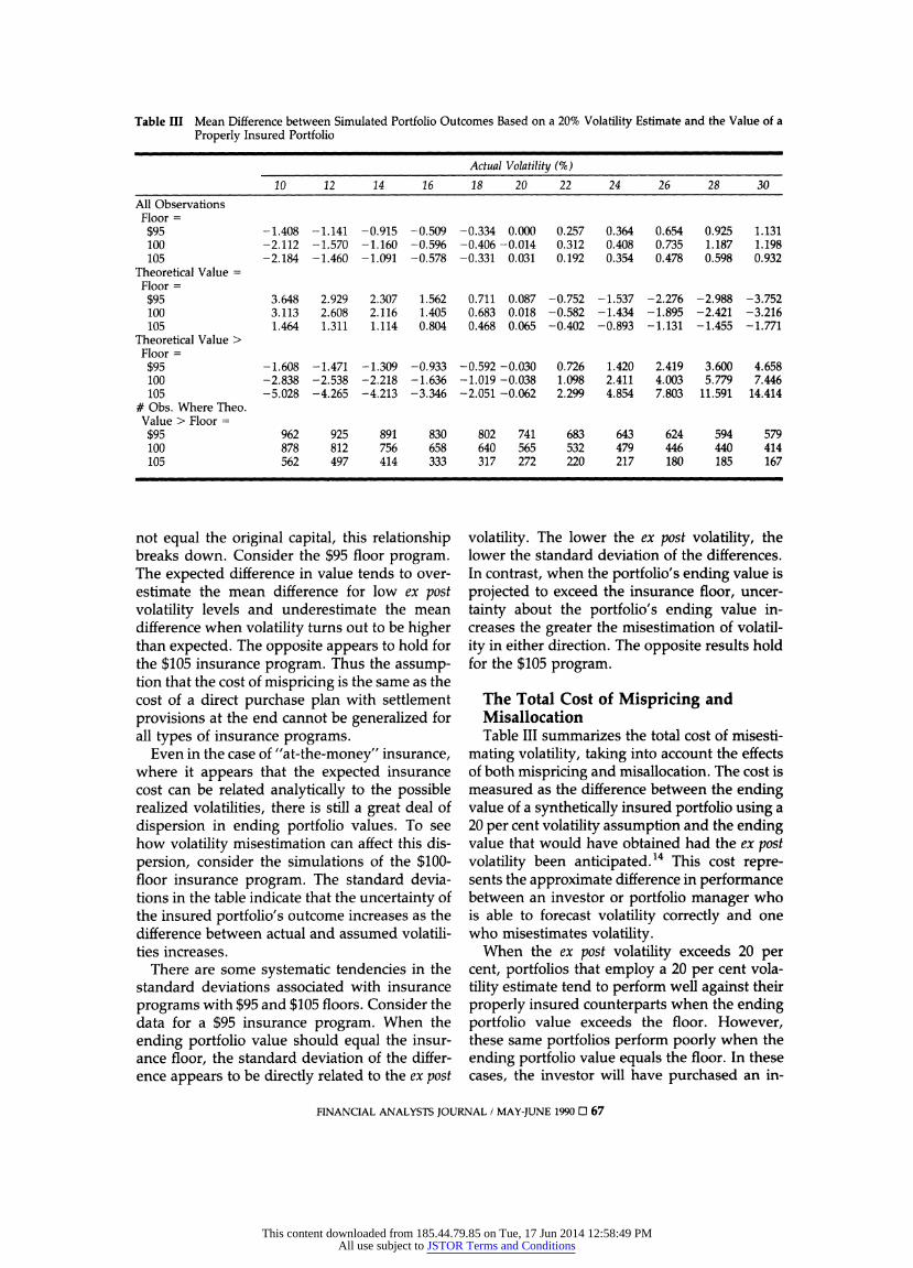
Table III Mean Difference between Simulated Portfolio Outcomes Based on a 20% Volatility Estimate and the Value of a Properly Insured Portfolio

Actual Volatility (%)

10 12 14 16 18 20 22 24 26 28 30

All Observations Floor = $95 -1.408 -1.141 -0.915 -0.509 -0.334 0.000 0.257 0.364 0.654 0.925 1.131 100 -2.112 -1.570 -1.160 -0.596 -0.406 -0.014 0.312 0.408 0.735 1.187 1.198 105 -2.184 -1.460 -1.091 -0.578 -0.331 0.031 0.192 0.354 0.478 0.598 0.932

Theoretical Value = Floor = $95 3.648 2.929 2.307 1.562 0.711 0.087 -0.752 -1.537 -2.276 -2.988 -3.752 100 3.113 2.608 2.116 1.405 0.683 0.018 -0.582 -1.434 -1.895 -2.421 -3.216 105 1.464 1.311 1.114 0.804 0.468 0.065 -0.402 -0.893 -1.131 -1.455 -1.771

Theoretical Value > Floor = $95 -1.608 -1.471 -1.309 -0.933 -0.592 -0.030 0.726 1.420 2.419 3.600 4.658 100 -2.838 -2.538 -2.218 -1.636 -1.019 -0.038 1.098 2.411 4.003 5.779 7.446 105 -5.028 -4.265 -4.213 -3.346 -2.051 -0.062 2.299 4.854 7.803 11.591 14.414

# Obs. Where Theo. Value > Floor = $95 962 925 891 830 802 741 683 643 624 594 579 100 878 812 756 658 640 565 532 479 446 440 414 105 562 497 414 333 317 272 220 217 180 185 167

not equal the original capital, this relationship breaks down. Consider the $95 floor program. The expected difference in value tends to over- estimate the mean difference for low ex post volatility levels and underestimate the mean difference when volatility turns out to be higher than expected. The opposite appears to hold for the $105 insurance program. Thus the assumption that the cost of mispricing is the same as the cost of a direct purchase plan with settlement provisions at the end cannot be generalized for all types of insurance programs.

Even in the case of "at-the-money" insurance, where it appears that the expected insurance cost can be related analytically to the possible realized volatilities, there is still a great deal of dispersion in ending portfolio values. To see how volatility misestimation can affect this dispersion, consider the simulations of the $100- floor insurance program. The standard deviations in the table indicate that the uncertainty of the insured portfolio's outcome increases as the difference between actual and assumed volatilities increases.

There are some systematic tendencies in the standard deviations associated with insurance programs with $95 and $105 floors. Consider the data for a $95 insurance program. When the ending portfolio value should equal the insurance floor, the standard deviation of the difference appears to be directly related to the ex post

volatility. The lower the ex post volatility, the lower the standard deviation of the differences. In contrast, when the portfolio's ending value is projected to exceed the insurance floor, uncertainty about the portfolio's ending value increases the greater the misestimation of volatility in either direction. The opposite results hold for the $105 program.

The Total Cost of Mispricing and Misallocation Table III summarizes the total cost of misesti-

mating volatility, taking into account the effects of both mispricing and misallocation. The cost is measured as the difference between the ending value of a synthetically insured portfolio using a 20 per cent volatility assumption and the ending value that would have obtained had the ex post volatility been anticipated.14 This cost represents the approximate difference in performance between an investor or portfolio manager who is able to forecast volatility correctly and one who misestimates volatility.

When the ex post volatility exceeds 20 per cent, portfolios that employ a 20 per cent volatility estimate tend to perform well against their properly insured counterparts when the ending portfolio value exceeds the floor. However, these same portfolios perform poorly when the ending portfolio value equals the floor. In these cases, the investor will have purchased an in-




Table IV S&P 500 Values Over the Period October 5, 1987 to November 9, 1987

Date S&P Value (000$) S&P Return (%) 10-05-87 328.08 N/A 10-12-87 309.39 -5.697 10-19-87 224.84 -27.328 10-26-87 227.67 1.259 11-02-87 255.75 12.334 11-09-87 243.17 -4.919

sufficient amount of insurance. Naturally, subsequent performance will be better than expected when insurance turns out not to have been needed.

Conversely when an investor overestimates volatility, he purchases too much insurance. Accordingly, portfolio performance will look bad when the underlying portfolio subse- quently performs well. Of course, if subsequent conditions justify the incremental insurance, performance will exceed expectations.

By purchasing too much insurance, the investor actually increases the likelihood that the insurance will come into effect. For example, Table II shows that insurance should come into play in 308 of 1,000 simulations for a $100 floor program when the ex post volatility turns out to be 10 per cent. However, if the same portfolio is insured properly, Table III shows that the floor should be reached only 122 (1,000 - 878) times. Thus the misestimation of volatility not only affects the ending value of an insured portfolio, it also affects the likelihood that insurance will be needed.

Simulations Under Crash Conditions It is well known that the stock market crash of October 1987 adversely affected the performance of most synthetic option-replication portfolio insurance plans. Clearly, no portfolio manager could have anticipated such a dramatic change in stock market volatility and built such expectations into a portfolio insurance program that was already underway. It is nevertheless interesting to consider how much of an adverse impact the crash would have had on simulated portfolio results.15

We defined the relevant period for the stock market crash as the five-week period beginning at the close of trading on Monday, October 5 and going through the close on Monday, No- vember 9. Through both visual inspection of stock market data and quantitative measure-

ment of volatility, it is clear that this particular five-week period exhibited far greater volatility than prior periods, and with the exception of one day in late November and two days in early January 1988, the stock market had essentially returned to normal by November 9. Table IV presents closing S&P 500 values for each Mon- day over the five-week crash period; we used these values as typical stock portfolio values during the crash.

To estimate the potential effect of the crash on portfolio performance, we ran our simulations again, assuming that synthetic portfolio insurance was maintained under a 20 per cent volatility assumption and that, except for the five- week crash period, actual volatility was 20 per cent. 16 In an effort to simulate the stock market crash, we randomly selected one week in each simulation as the start of the five-week crash period. If this randomly selected week was any of weeks 1 through 48, we substituted crash- period returns from Table IV for each of the next five weeks, but assumed volatility returned to a normal 20 per cent after the five-week period. If the randomly selected week was any of weeks 49 through 52, we simply substituted crash returns beginning in the week of October 5, 1987 through October 12, 1987 and continued substituting such returns through the remaining life of the insurance program. By using this method, we were able to take into account the fact that most insurance programs would have felt the full force of the crash, while some programs may have terminated prior to the end of the five-week crash period.

Table V summarizes the results. In all in- stances, the performance of the underlying stock portfolio was so bad that the ending portfolio value should equal the guaranteed floor; that is, the insurance should have gone into effect. The table shows that, for a guaranteed floor of $100 per $100 of initial capital, the typical insured portfolio fell $16.680 short of its promised value. In one instance, the ending

Table V Simulations of Portfolio Insurance Performance in the October 1987 Stock Market Crash (based on 1,000 simulations)

Floor = $95 Floor = $100 Floor = $105

Mean Difference -20.034 -16.680 -8.143 Max. Difference 1.111 1.586 1.314 Min. Difference - 39. 672 - 40.402 - 41 .888 Std. Deviation 7.832 9.645 9.038




value fell approximately $40 below the floor, and in one outcome the ending value was almost $1.60 above the floor. With a guaranteed floor of only $95, average performance was even worse: A typical portfolio fell approximately $20 short of its promised value. With a $105 floor, performance was much better, the value of the average portfolio being only $8.143 below its guaranteed value.

The reason for these results is simple: With a low guaranteed floor, a smaller portion of the portfolio is invested in insurance. As a result, such portfolios are managed more aggressively than the others and therefore perform worse during a catastrophic period such as the October 1987 market crash.

We should point out that our crash scenario results may be somewhat overstated. Our analysis assumes weekly revisions in the stock/T-bill mix of synthetically insured portfolios. In prac- tice, many portfolio managers make revisions based on specific dollar changes in the value of the stock portfolio being insured. Clearly, such portfolio revisions would have been more fre- quent during the crash period, and therefore the portfolios might not have experienced losses as large as those reported in Table V.

Conclusions The misestimation of volatility can have a significant impact on the ending payoffs of portfolios that are insured synthetically. However, our simulations are somewhat limited in scope. They assume constant volatility, no revisions in volatility estimates, weekly portfolio revisions and stock prices that evolve according to specific probability distributions. Moreover, our simulations pertain only to pure option-replicating insurance programs. Consequently, while our simulations provide a useful understanding of the effects of volatility misestimation, actual portfolio performance may deviate significantly from our simulation results. U

Footnotes 1. See M. Rubinstein and H. Leland, "Replicating

Options with Positions in Stock and Cash," Fi- nancial Analysts Journal, July/August 1981.

2. M. Asay and C. Edelsberg, "Can a Dynamic Strategy Replicate the Returns of an Option?" Journal of Futures Markets, Spring 1986.

3. J. Hill, A. Jain and R. Wood, "Insurance: Volatil- ity Risk and Futures Mispricing," Journal of Port- folio Management, Winter 1988.

4. C. Garcia and F. Gould, "An Empirical Study of

Portfolio Insurance," Financial Analysts Journal, July/August 1987.

5. S. Figlewski, "Options Arbitrage in Imperfect Markets" (Paper presented at the American Stock Exchange Option Colloquium, 1988).

6. If all dividends are reinvested and the dividend payments reduce stock prices by their amounts, the dollar amount of risky assets under management will be the same as if no dividends had been paid; as a result, the costs associated with insuring both types of portfolios should be the same.

7. F. Black and M. Scholes, "The Pricing of Options and Corporate Liabilities," Journal of Political Economy, May-June 1973.

8. See Asay and Edelsberg, "Can a Dynamic Strat- egy," op. cit., Hill et al., "Insurance," op. cit., and T. O'Brien, "Portfolio Insurance Mechanics," Journal of Portfolio Management, Spring 1988.

9. We thank Dwight Grant for suggesting this method of presentation.

10. $4.62 is the Black-Scholes value of a one-year, $100-striking-price put on $91.73 of stock.

11. Our assumptions of a 15 per cent expected return for stock and a 7 per cent T-bill return are consistent with a historical risk premium of approximately 8 per cent. Note that the ex post volatility in a given simulation may deviate from the volatility assumed in generating random stock returns. In a given simulation, for example, random stock prices could be generated as if the return volatility is 30 per cent, while actual volatility of the random stock returns turns out to be dispersed around 30 per cent; this is a result of sampling error.

12. The N(dl) term of Equation (2) is used to deter- mine the number of shares of stock that should be held at the beginning of each period. Any remaining funds are assumed to be invested in T-bills. If the stock investment exceeds the portfolio's equity, the difference is made up by bor- rowing at the T-bill rate.

13. Time-based revision programs can be related to those whose revisions are based on price move- ments. If one makes revisions whenever the return on the underlying stock equals or exceeds its weekly mean plus or minus its weekly standard deviation, for example, then the average revision period will be one week. We have found that it makes little difference which method is used, as long as the rule for price-change-based revisions is consistent with the time-based rule. Our results, derived by our research assistant Phillip Davis, are available upon request.

14. The analysis assumes no uncertainty, conditional on the ending stock value, in the payoff of the insurance program that employs the correct volatility. Thus the insurance component of this




portfolio is assumed to be purchased directly, rather than synthetically.

15. Y. Zhu and R. Kavee ("Performance of Portfolio Insurance Strategies," Journal of Portfolio Manage- ment, Spring 1988) simulated jumps in security prices and showed that such jumps could affect the guaranteed floor. Their analysis did not specifically address the 1987 crash.

16. We performed the same experiment using ex ante and ex post volatility assumptions ranging from 10 to 30 per cent and found little difference in the results.

Glossary Synthetic Option-Replicating Portfolio Insurance:

Of the several known strategies for setting a floor on portfolio losses, one is to create a put option on

the portfolio via a trading program (synthetic option replication).

Mispricing Effect: The misestimation of the cost of option replication due to misestimation of volatility.

European Puts: A European put is a put option that cannot be exercised prior to its expiration, as op- posed to an American option, which can be exercised prior to its expiration.

Volatility: The standard deviation of the rate of return.

Simulation: Simulation is the use of a model in "what if" fashion, with a wide range of inputs and often with a computer, when the model is too complex to employ in simple equation form.

Pure Option-Replicating Insurance: Same as synthetic option-replicating portfolio insurance (see above).




the effects of volatility misestimation on option-replication portfolio insurance

Documents