RESEARCH ARTICLE

The effect of geometry on ice shelf ocean cavity ventilation:a laboratory experiment

A. A. Stern • D. M. Holland • P. R. Holland •

A. Jenkins • J. Sommeria

Received: 30 May 2013 / Revised: 3 February 2014 / Accepted: 2 April 2014 / Published online: 20 April 2014

� Springer-Verlag Berlin Heidelberg 2014

Abstract A laboratory experiment is constructed to sim-

ulate the density-driven circulation under an idealized Ant-

arctic ice shelf and to investigate the flux of dense and

freshwater in and out of the ice shelf cavity. Our results

confirm that the ice front can act as a dynamic barrier that

partially inhibits fluid from entering or exiting the ice shelf

cavity, away from two wall-trapped boundary currents. This

barrier results in a density jump across the ice front and in the

creation of a zonal current which runs parallel to the ice front.

However despite the barrier imposed by the ice front, there is

still a significant amount of exchange of water in and out of

the cavity. This exchange takes place through two dense and

fresh gravity plumes which are constrained to flow along the

sides of the domain by the Coriolis force. The flux through

the gravity plumes and strength of the dynamic barrier are

shown to be sensitive to changes in the ice shelf geometry

and changes in the buoyancy fluxes which drive the flow.

1 Introduction

The Greenland and Antarctic ice sheets are comprised of

many separate ice streams, fast-flowing rivers of ice that

flow downhill under gravity. Where these ice streams come

into contact with the oceans, they either fracture and calve

icebergs, or they form ice shelves, large floating glaciers

that can be several kilometers thick and several hundreds of

kilometers wide.

The dynamics of the water within ice shelf cavities and

the flux of dense water in and out of the ice shelf cavities has

a strong influence on the calving and melting rates of the ice

shelves. However, the large quantity of ice above the cav-

ities has made observational measurements extremely dif-

ficult, and as a result, there exists relatively little data about

the circulation within the cavities. In addition to this, the

sloping and melting upper boundary above the cavity has a

strong effect on the dynamics of the flow within the cavity

and makes the dynamics distinct from all other ocean flows.

Nevertheless, in the past 30 years, a small body of

observational measurements under the Antarctic ice

shelves has begun to be created (e.g., Nicholls 1996; Ma-

kinson et al. 2005, 2006; Nicholls et al. 2009; Hattermann

et al. 2012; Jenkins et al. 2012) and a general picture of

dominant dynamical processes which take place within the

ice shelf cavities has begun to emerge. The first one-

dimensional models to describe ocean–ice interactions

within the Antarctic ice shelf cavities were put forward by

MacAyeal (1984, 1985) and Jenkins (1991) and later

extended to a 2-D model by Holland and Feltham (2006).

This model can be summarized as follows (Fig. 1). The

cold Antarctic winter conditions cause the surface water at

the ice front to freeze. The salt rejected during freezing

mixes with the cold ambient surface water to form high

salinity shelf water (HSSW). The dense HSSW sinks to the

bottom of the water column and flows down into the ice

shelf cavity toward the grounding line.

Since the freezing point of seawater decreases with

depth, the temperature of the HSSW, which was formed at

A. A. Stern (&) � D. M. Holland

Courant Institute of Mathematical Science, New York

University, New York, NY 10012, USA

e-mail: sternalon@gmail.com

P. R. Holland � A. Jenkins

British Antarctic Survey, High Cross, Madingley Road,

Cambridge CB3 0ET, UK

J. Sommeria

LEGI, CNRS, University of Grenoble-Alpes, 38000 Grenoble,

France

123

Exp Fluids (2014) 55:1719

DOI 10.1007/s00348-014-1719-3

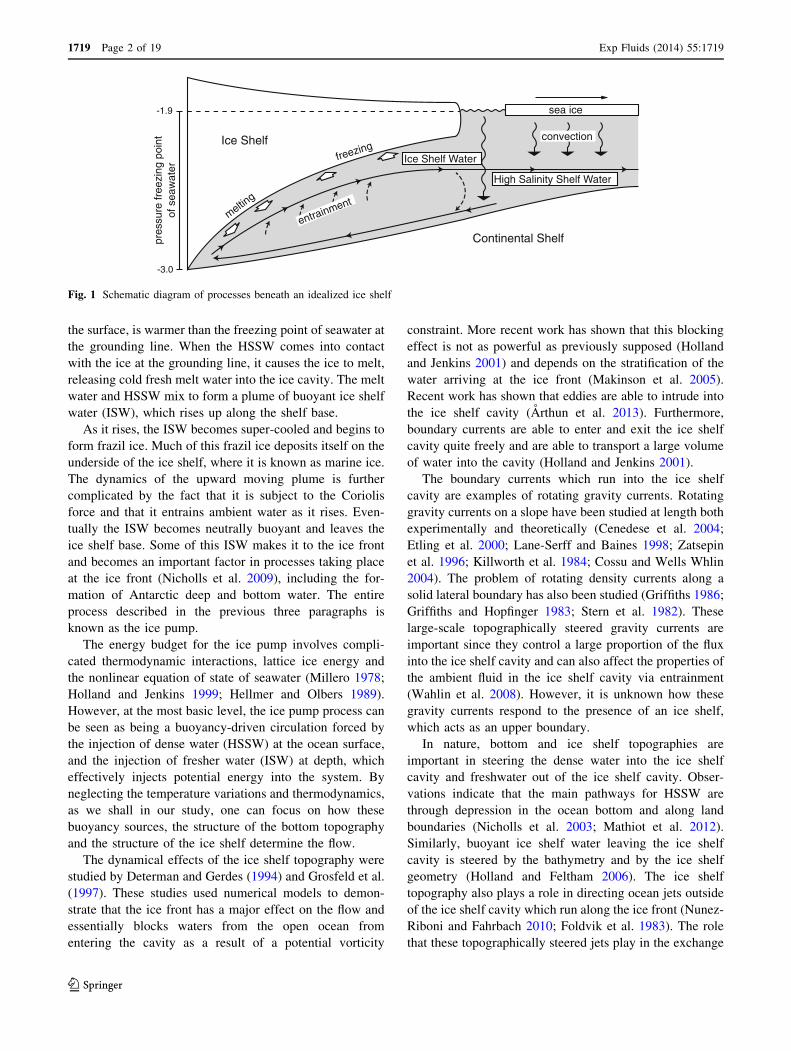
the surface, is warmer than the freezing point of seawater at

the grounding line. When the HSSW comes into contact

with the ice at the grounding line, it causes the ice to melt,

releasing cold fresh melt water into the ice cavity. The melt

water and HSSW mix to form a plume of buoyant ice shelf

water (ISW), which rises up along the shelf base.

As it rises, the ISW becomes super-cooled and begins to

form frazil ice. Much of this frazil ice deposits itself on the

underside of the ice shelf, where it is known as marine ice.

The dynamics of the upward moving plume is further

complicated by the fact that it is subject to the Coriolis

force and that it entrains ambient water as it rises. Even-

tually the ISW becomes neutrally buoyant and leaves the

ice shelf base. Some of this ISW makes it to the ice front

and becomes an important factor in processes taking place

at the ice front (Nicholls et al. 2009), including the for-

mation of Antarctic deep and bottom water. The entire

process described in the previous three paragraphs is

known as the ice pump.

The energy budget for the ice pump involves compli-

cated thermodynamic interactions, lattice ice energy and

the nonlinear equation of state of seawater (Millero 1978;

Holland and Jenkins 1999; Hellmer and Olbers 1989).

However, at the most basic level, the ice pump process can

be seen as being a buoyancy-driven circulation forced by

the injection of dense water (HSSW) at the ocean surface,

and the injection of fresher water (ISW) at depth, which

effectively injects potential energy into the system. By

neglecting the temperature variations and thermodynamics,

as we shall in our study, one can focus on how these

buoyancy sources, the structure of the bottom topography

and the structure of the ice shelf determine the flow.

The dynamical effects of the ice shelf topography were

studied by Determan and Gerdes (1994) and Grosfeld et al.

(1997). These studies used numerical models to demon-

strate that the ice front has a major effect on the flow and

essentially blocks waters from the open ocean from

entering the cavity as a result of a potential vorticity

constraint. More recent work has shown that this blocking

effect is not as powerful as previously supposed (Holland

and Jenkins 2001) and depends on the stratification of the

water arriving at the ice front (Makinson et al. 2005).

Recent work has shown that eddies are able to intrude into

the ice shelf cavity (Arthun et al. 2013). Furthermore,

boundary currents are able to enter and exit the ice shelf

cavity quite freely and are able to transport a large volume

of water into the cavity (Holland and Jenkins 2001).

The boundary currents which run into the ice shelf

cavity are examples of rotating gravity currents. Rotating

gravity currents on a slope have been studied at length both

experimentally and theoretically (Cenedese et al. 2004;

Etling et al. 2000; Lane-Serff and Baines 1998; Zatsepin

et al. 1996; Killworth et al. 1984; Cossu and Wells Whlin

2004). The problem of rotating density currents along a

solid lateral boundary has also been studied (Griffiths 1986;

Griffiths and Hopfinger 1983; Stern et al. 1982). These

large-scale topographically steered gravity currents are

important since they control a large proportion of the flux

into the ice shelf cavity and can also affect the properties of

the ambient fluid in the ice shelf cavity via entrainment

(Wahlin et al. 2008). However, it is unknown how these

gravity currents respond to the presence of an ice shelf,

which acts as an upper boundary.

In nature, bottom and ice shelf topographies are

important in steering the dense water into the ice shelf

cavity and freshwater out of the ice shelf cavity. Obser-

vations indicate that the main pathways for HSSW are

through depression in the ocean bottom and along land

boundaries (Nicholls et al. 2003; Mathiot et al. 2012).

Similarly, buoyant ice shelf water leaving the ice shelf

cavity is steered by the bathymetry and by the ice shelf

geometry (Holland and Feltham 2006). The ice shelf

topography also plays a role in directing ocean jets outside

of the ice shelf cavity which run along the ice front (Nunez-

Riboni and Fahrbach 2010; Foldvik et al. 1983). The role

that these topographically steered jets play in the exchange

Ice Shelf

Continental Shelf

entrainment

freezing

melting

convection

Ice Shelf Water

High Salinity Shelf Water

-1.9

-3.0

pres

sure

free

zing

poi

ntof

sea

wat

er

sea ice

Fig. 1 Schematic diagram of processes beneath an idealized ice shelf

1719 Page 2 of 19 Exp Fluids (2014) 55:1719

123

of water into and out of the cavity is still unknown. In real-

world ice shelves, easterly winds at the ice front are

involved in driving the jet, which further complicates the

dynamics.

In this study, a laboratory experiment is created to

simulate the density-driven currents involved in the ice

pump. The first aim of the experiment was to observe how

water passes into and out of the ice shelf cavity and esti-

mate the flux of dense water which moves into the cavity as

a gravity plume along the lateral boundary. Secondly, the

experiment aimed to determine how the flux of dense water

into the cavity, the flux of freshwater out of the cavity, the

circulation inside the cavity and the structure of the gravity

plumes moving into and out of the cavity are affected by

varying the buoyancy fluxes injected into the system, and

varying the geometry of the ice shelf cavity.

In the experiment described below, the flow was visu-

alized using particle image velocimetry (PIV) (Adrian

2005) and laser-induced fluorescence (LIF) (Houcine et al.

1996). Recent advancements in flow visualization in lab-

oratory experiments have meant that laboratory experi-

ments can be used for quantitative rather than qualitative

geophysical applications. However, in recent years, the use

of laboratory experiments to study ocean–ice interaction

has not been popular. One of the purposes of this study is to

present observations and lessons from a first effort

obtaining quantitative data to help understand sub-ice shelf

circulation.

Section 2 explains the experimental setup, measurement

methods and calibration process. The results of the

experiments are outlined in Sect. 3. Section 4 contains a

brief discussion of the results. Section 5 contains some

concluding remarks.

2 Experimental setup and data collection

The experiment described below was performed on a

rotating platform in the Coriolis laboratory, in Grenoble,

France. In this section, we explain the experimental setup,

the different types of experimental runs and comment on

the data collected.

2.1 Experimental setup

The experimental setup was motivated by the descriptions

of the ‘‘ice pump’’ described in the introduction (MacAyeal

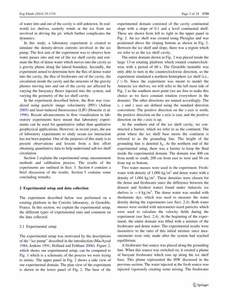
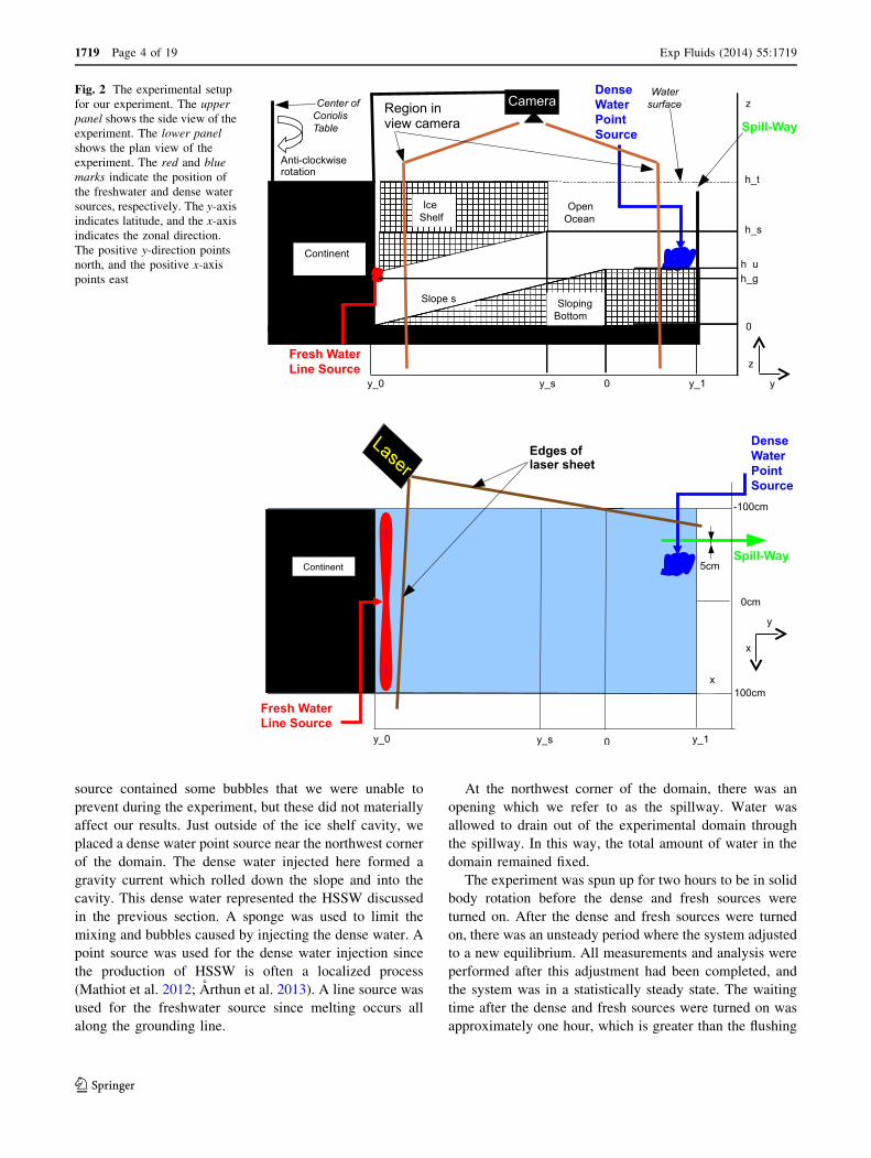
1984; Jenkins 1991; Holland and Feltham 2006). Figure 2,

which shows our experimental setup, can be compared to

Fig. 1 which is a schematic of the process we were trying

to mimic. The upper panel in Fig. 2 shows a side view of

our experimental domain. The plan view of the experiment

is shown in the lower panel of Fig. 2. The base of the

experimental domain consisted of the cavity continental

slope with a slope of 0.1 and a level continental shelf.

These are shown from left to right in the upper panel in

Fig. 2. An ice shelf was created using Plexiglas and was

positioned above the sloping bottom as shown in Fig. 2.

Between the ice shelf and slope, there was a region which

we refer to as the ice shelf cavity.

The entire domain shown in Fig. 2 was placed inside the

large 13-m rotating platform which rotated counterclock-

wise with a period of 60 s. The Grenoble turntable was

only able to turn in the counterclockwise direction, so the

experiment simulated a northern hemisphere ice shelf (i.e.,

f [ 0). Since the experiment was meant to model the

Antarctic ice shelves, we will refer to the left most side of

Fig. 2 as the southern most point (we are free to make this

choice as we have constant rotation everywhere in the

domain). The other directions are named accordingly. The

x, y and z axes are defined using the standard direction

convention: The positive direction on the y-axis is north,

the positive direction on the x-axis is east, and the positive

direction on the z-axis is up.

At the southern end of the ice shelf cavity, we con-

structed a barrier, which we refer to as the continent. The

point where the ice shelf base meets the continent is

referred to as the grounding line. The height of the

grounding line is denoted hg. At the northern end of the

experimental setup, there was a barrier to keep the fluid

inside the experimental domain. The domain was 400 cm

from north to south, 200 cm from east to west and 56 cm

from top to bottom.

Two water masses were used in the experiment: Fresh-

water with density of 1,000 kg=m3 and dense water with a

density of 1,004 kg=m3. These densities were chosen for

the dense and freshwater since the difference between the

densest and freshest waters found under Antarctic ice

shelves is � 4 kg=m3. The dense water was seeded with

rhodamine dye, which was used to measure the water

density during the experiments (see Sect. 2.4). Both water

masses were seeded with micrometer-sized particles which

were used to calculate the velocity fields during the

experiment (see Sect. 2.4). At the beginning of the exper-

iment, the entire domain was filled with a mixture of the

freshwater and dense water. The experimental results were

insensitive to the ratio of this initial mixture since mea-

surements were only made after the system had reached

equilibrium.

A freshwater line source was placed along the grounding

line. When this source was switched on, it created a plume

of buoyant freshwater which rose up along the ice shelf

base. This plume represented the ISW discussed in the

previous section. The water injected at the fresh source was

injected vigorously creating some mixing. The freshwater

Exp Fluids (2014) 55:1719 Page 3 of 19 1719

123

source contained some bubbles that we were unable to

prevent during the experiment, but these did not materially

affect our results. Just outside of the ice shelf cavity, we

placed a dense water point source near the northwest corner

of the domain. The dense water injected here formed a

gravity current which rolled down the slope and into the

cavity. This dense water represented the HSSW discussed

in the previous section. A sponge was used to limit the

mixing and bubbles caused by injecting the dense water. A

point source was used for the dense water injection since

the production of HSSW is often a localized process

(Mathiot et al. 2012; Arthun et al. 2013). A line source was

used for the freshwater source since melting occurs all

along the grounding line.

At the northwest corner of the domain, there was an

opening which we refer to as the spillway. Water was

allowed to drain out of the experimental domain through

the spillway. In this way, the total amount of water in the

domain remained fixed.

The experiment was spun up for two hours to be in solid

body rotation before the dense and fresh sources were

turned on. After the dense and fresh sources were turned

on, there was an unsteady period where the system adjusted

to a new equilibrium. All measurements and analysis were

performed after this adjustment had been completed, and

the system was in a statistically steady state. The waiting

time after the dense and fresh sources were turned on was

approximately one hour, which is greater than the flushing

z

z

Fig. 2 The experimental setup

for our experiment. The upper

panel shows the side view of the

experiment. The lower panel

shows the plan view of the

experiment. The red and blue

marks indicate the position of

the freshwater and dense water

sources, respectively. The y-axis

indicates latitude, and the x-axis

indicates the zonal direction.

The positive y-direction points

north, and the positive x-axis

points east

1719 Page 4 of 19 Exp Fluids (2014) 55:1719

123

time for the system, Tf , and the spin-up time, Ts (see

Sect. 2.2.1). Measurements of the density-driven circula-

tion were observed using a camera positioned above the

experimental domain. In the different experimental runs,

measurements were taken for between 4,000 and 10,000 s.

Three tests were performed to explore the effect of ice

geometry and buoyancy sources on the ice shelf

circulation:

• Thickness investigation The thickness of the ice shelf

cavity was varied, while the slope of the ice shelf and

the buoyancy sources were kept constant.

• Gradient investigation The gradient of the ice shelf was

varied, while the buoyancy sources were kept constant.

• Buoyancy investigation The buoyancy sources were

varied, while the ice shelf geometry was kept constant.

In the rest of the paper, we refer to these three investiga-

tions as the thickness investigation, gradient investigation

and buoyancy investigation. The term experimental runs is

used throughout the rest of the paper to refer to individual

simulations which made up these three investigations. Each

investigation consisted of three experimental runs. The

number of experimental runs was limited by the time taken

to run an experiment and the complexity of the experi-

mental setup. The same Control Run was used for all three

investigations meaning that in total, seven different

experimental runs were performed.

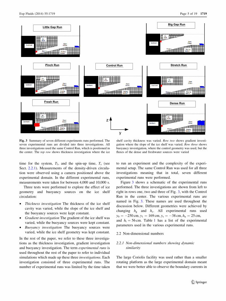
Figure 3 shows a schematic of the experimental runs

performed. The three investigations are shown from left to

right in rows one, two and three of Fig. 3, with the Control

Run in the center. The various experimental runs are

named in Fig. 3. These names are used throughout the

discussion below. Different geometries were achieved by

changing hg and hs. All experimental runs used

y0 ¼ �250 cm; y1 ¼ 169 cm; ys ¼ �38 cm; hu ¼ 25 cm,

and ht ¼ 56 cm. Table 1 has a list of the experimental

parameters used in the various experimental runs.

2.2 Non-dimensional numbers

2.2.1 Non-dimensional numbers showing dynamic

similarity

The large Coriolis facility was used rather than a smaller

rotating platform as the large experimental domain meant

that we were better able to observe the boundary currents in

Fig. 3 Summary of seven different experiments runs performed. The

seven experimental runs are divided into three investigations. All

three investigations used the same Control Run, which is positioned in

the center. The top row shows thickness investigation where the ice

shelf cavity thickness was varied. Row two shows gradient investi-

gation where the slope of the ice shelf was varied. Row three shows

buoyancy investigation, where the control geometry was used, but the

fluxes of the dense and freshwater sources were varied

Exp Fluids (2014) 55:1719 Page 5 of 19 1719

123

the experiment, with the limited resolution of our mea-

surements. The largeness of experimental domain also

allowed us to achieve non-dimensional numbers which

were more similar to the real world.

The Rossby number of our system was

R0 ¼ UfL¼ 10�2

0:2�1 ¼ 120

. Here we use the fact that

f ¼ 4pT¼ 4p

60� 0:2. We use L = 1 m, which half of the

width of the domain and U ¼ 10�2 m/s, which was a typ-

ical velocity observed in the experiments. The real-world

Rossby number can be estimated as Rocean ¼ UfL� 10�1

10�4�105 ¼10�2 where the estimate of U comes from Nicholls (1996).

The smallness of the Rossby number in both cases means

that the system was likely to be close to geostrophic

balance.

Since we were using a large tank, we were able to

achieve a small aspect ratio a0 ¼ HL� 0:5 m

4 m� 10�1. The

length of the tank was 4m. The aspect ratio of the real-

world ice cavities is aocean � 103 m105 m¼ 10�2. While our

aspect ratio is an order of magnitude larger than that of the

ocean, both systems are strongly influenced by the small-

ness of their aspect ratio.

The frictional Ekman layer thickness scales like

d ¼ffiffi

mf

q

. Using the viscosity of water m � 10�6 m2=s1, we

estimate a molecular Ekman layer thickness of

dmol ¼ffiffi

mf

q

�ffiffiffiffiffiffiffi

10�6

15

q

¼ 2:2� 10�3 m ¼ 2:2 mm. This pro-

vides a lower bound of the Ekman layer thickness. To get

an upper bound on the Ekman layer thickness, we use a

typical Eddy viscosity found in the ocean, m ¼ 10�2. This

gives us dtur ¼ffiffi

mf

q

�ffiffiffiffiffiffiffi

10�2

15

q

¼ 22 cm. However, since our

system was likely to be much less turbulent than the ocean,

it is probable that the eddy viscosity will be an order of

magnitude or more smaller, resulting in an Ekman layer

thickness, d, between 1 and 10 cm, although this is hard to

predict a priori. In the experimental results shown below,

the Ekman boundary layer cannot be seen. This is espe-

cially apparent in the dense and fresh plumes where the

fastest speeds are close to the lower and upper boundaries,

respectively. This implies that the Ekman layer thickness is

likely to be smaller than 2 cm, the resolution of the

velocity measurements.

The Reynolds number in the experiment is

Re ¼ ULm ¼ 10�2�1

10�6 ¼ 104. Since the transition to turbulence

typically occurs for 2;300\Re\4;000 (in a pipe flow)

(Holman 2002), the fluid in our experiment was likely to

have been turbulent. While the Reynolds number is smaller

than typical Reynolds numbers found in the ocean, it is

comparable to Reynolds numbers used in numerical mod-

els. The Froude number for the gravity plumes in the

experiment is F ¼ Uffiffiffiffiffiffi

g0Hp ¼ 10�2

ffiffiffiffiffiffiffiffiffiffiffiffiffiffiffi

10�2�10�1p � 0:3, which is

slightly subcritical.

The spin-up time for a rotating tank is T ¼ffiffiffiffiffiffiffiffi

L2

m Xq

(Greenspan and Howard 1963). In our experiment, the

spin-up time is estimated as T ¼ffiffiffiffiffiffiffiffi

L2

m Xq

¼ffiffiffiffiffiffiffiffiffiffiffiffiffiffiffiffiffiffiffi

1 m2

10�6 m2=s12p60

q

� 1072s � 3; 000s. The experiments were

allowed to spin up for 2 h to reach solid body rotation

before the flow was turned on. The experimental domain

contained � 2 m3 of water. The combined flux of the dense

water and freshwater sources was 40 l/m

(�0:66� 10�3 m3=s). This meant that the flushing time for

the system was Tf � 3;000 s.

2.2.2 Non-dimensional parameters varied in experiments

The changes in geometry and buoyancy used in the three

investigations can be described by three non-dimensional

numbers: Gt;Gs and Gb. These are described below:

We define Gt as the ratio of the thickness of the water

column inside and outside the ice shelf cavity at the ice

front. Since the height of the ocean floor at the ice front is

hu � jysjs, we define

Gt ¼hs � ðhu � jysjsÞht � ðhu � jysjsÞ

ð1Þ

Here s is the slope of the ocean bottom. Gt gives a measure

of the change of water column thickness which occurs as a

column of fluid moves across the ice front.

Gs is defined to be the average meridional gradient of

the ice cavity thickness. In our setup, Gs is given by

Gs ¼ðhg � 0Þ � ðhs � ðhu � jysjsÞÞ

jy0 � ysjð2Þ

Gs gives a measure of how the cavity water column

thickness changes as a column of fluid moves from the

grounding line to the ice front.

Gb is defined as the ratio of the mass flux anomaly

caused by injecting dense and freshwater into the system.

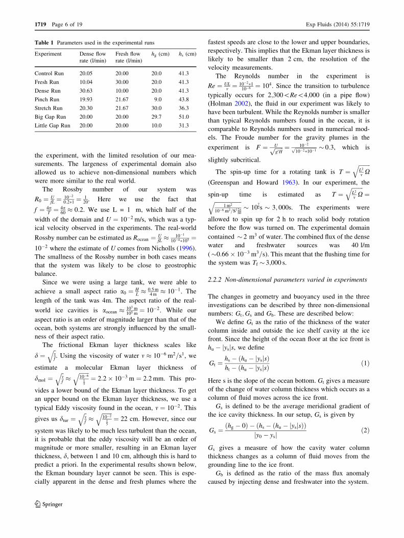
Table 1 Parameters used in the experimental runs

Experiment Dense flow

rate (l/min)

Fresh flow

rate (l/min)

hg (cm) hs (cm)

Control Run 20.05 20.00 20.0 41.3

Fresh Run 10.04 30.00 20.0 41.3

Dense Run 30.63 10.00 20.0 41.3

Pinch Run 19.93 21.67 9.0 43.8

Stretch Run 20.30 21.67 30.0 36.3

Big Gap Run 20.00 20.00 29.7 51.0

Little Gap Run 20.00 20.00 10.0 31.3

1719 Page 6 of 19 Exp Fluids (2014) 55:1719

123

Gb ¼DMd

DMf

ð3Þ

If the ambient water in the system has a density of qa, the

dense water has a density of qd, and the freshwater has a

density of qf , then the mass flux anomalies are given by

DMd ¼ ðqd � qaÞQd ð4Þ

DMf ¼ ðqa � qfÞQf ð5Þ

Here Qd and Qf are the fluxes of water injected at the

dense and fresh source, respectively. The density of the

dense water and freshwaters injected into the system

were, qd ¼ 1;004 kg=m3 and qd ¼ 1;000 kg=m3. We set

qa ¼ðqdþqfÞ

2¼ 1;002 kg=m3.

In the Control Run, we used Gt ¼ 0:58;Gs ¼ 0:00 and

Gb ¼ 1:0. Values were picked in order to make the Control

Run analogous to the Ross Ice Shelf. The average ice draft

of Ross Ice Shelf at the ice front is � 300 m, while the

continental shelf depth is � 700 m below sea level (Davey

2004). This gives Gt� 400 m700 m

� 0:57. At 180�W, the Ross

Ice Shelf cavity thickness changes by 300 m over a dis-

tance of 300 km between 79�S and 82�S (Davey 2004).

This implies Gs� 11;000

.

To calculate Gb; we use the freshwater flux in the Ross

Sea caused by sea ice production, evaporation, precipita-

tion and the basal melt beneath the Ross Ice Shelf. Ass-

mann et al. (2003) estimated the total flux of freshwater

from basal melt beneath the Ross Ice Shelf to be 5.3 mSv

(Assmann et al. 2003). The total freshwater flux on the

Ross Sea continental shelf (excluding the contribution of

melt water from under the ice shelf) was estimated to be

�26.6 mSv. Here 1 mSv ¼ 103 m3=s1. Taking the ratio,

this gives Gb� 5. However, a large portion of the dense

water created in the Ross Sea is exported off the conti-

nental shelf and does not influence the dynamics under the

ice shelf (Orsi et al. 2002; Gordon et al. 2009). Because of

this uncertainty in the total amount of freshwater extraction

which affects the ice shelf dynamics, we note that

Gb�Oð1Þ, and used Gb ¼ 1 in our Control Run. The

Dense Run and Fresh Run are used to examine the effect of

changes in Gb on the circulation beneath the ice shelf.

The values of Gt;Gs and Gb used in the three different

investigations are shown in Table 2. Values of Gt;Gs and

Gb were varied in order to examine the sensitivity of the

circulation to changes in these parameters. These experi-

ments are motivated by the fact that paleoclimate records

show that the geometry and basal melt of the Ross Ice Shelf

have changed significantly in the past (Conway et al.

1999). We are interested in how the circulation beneath the

Ross Ice Shelf might have responded to such changes.

Furthermore, these experiments are also of interest in

comparing different ice shelves around Antarctica, which

have differing geometries and buoyancy fluxes. The Ron-

ne–Filchner Ice Shelf, for example, has a large ice draft at

the ice front and therefore has a smaller value for Gt, while

the draft of the ice front of the McMurdo Ice Shelf is only

20 m, and hence Gt� 1 (Stern et al. 2013). Pine Island

Glacier has a large value for Gs since it has an ice shelf

which is many time steeper than the Ross Ice Shelf,

resulting in a large change of cavity thickness over a

shorter distance. Gs can also be negative locally when there

is steep bottom topography. The large flux of ISW asso-

ciated with rapidly melting ice shelve likely results in a

small value of Gb. Changing values of Gb could be relevant

to future climate change scenarios.

2.3 Data collected during the experiments

A camera was placed above the experimental domain, and

a laser was placed southwest of the domain (see Fig. 2).

The walls of the domain were constructed using Plexiglas

to allow the laser light to pass through. The laser created a

horizontal plane of light, which allowed the camera to take

pictures of the fluid illuminated by the laser. A mirror was

placed on a carriage which could move up and down, and

direct the laser light to different levels so that we were able

to get images in 23 different horizontal planes. The camera

position remained fixed 5 m above the experimental

domain, rotating with the table. The camera was suffi-

ciently far from the domain that the camera focus was not

significantly affected by moving the laser sheet. At each

level, 3 images were taken at a frequency of 3 Hz. The

images at different heights were taken 3 s apart. This

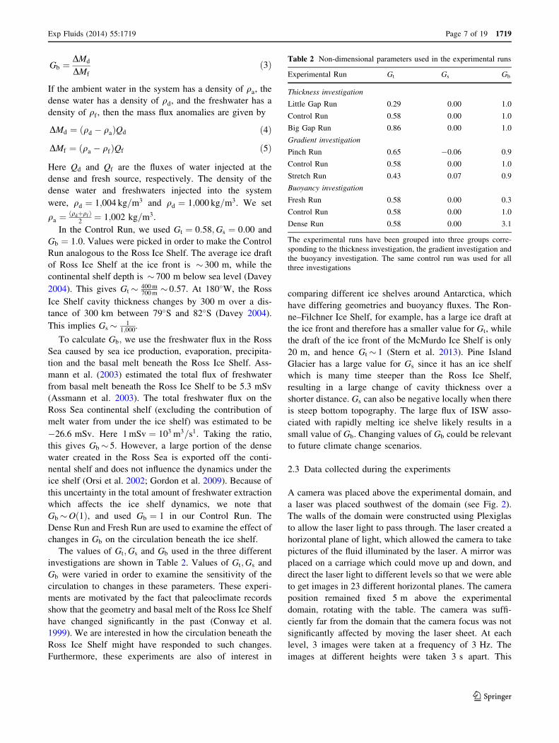
Table 2 Non-dimensional parameters used in the experimental runs

Experimental Run Gt Gs Gb

Thickness investigation

Little Gap Run 0.29 0.00 1.0

Control Run 0.58 0.00 1.0

Big Gap Run 0.86 0.00 1.0

Gradient investigation

Pinch Run 0.65 -0.06 0.9

Control Run 0.58 0.00 1.0

Stretch Run 0.43 0.07 0.9

Buoyancy investigation

Fresh Run 0.58 0.00 0.3

Control Run 0.58 0.00 1.0

Dense Run 0.58 0.00 3.1

The experimental runs have been grouped into three groups corre-

sponding to the thickness investigation, the gradient investigation and

the buoyancy investigation. The same control run was used for all

three investigations

Exp Fluids (2014) 55:1719 Page 7 of 19 1719

123

meant that the images at every horizontal plane had a time

separation of 69 s. The size of the region in the view of the

camera was 226 cm in the north–south direction and

200 cm in the east–west direction. The entire width of the

domain (including the plumes on both sides of the domain)

was in the sight of the camera, while just over half of the

length of the domain (from north to south) was captured by

the cameras. The fresh and dense sources were not in the

field of view.

The fluid in the experiment was seeded with microme-

ter-sized particles, and the dense water injected at the dense

source was mixed with a known concentration of rhoda-

mine dye. The rhodamine dye and the seeded particles

were illuminated by the laser and showed up in the images

captured by the camera. These images were used to per-

form PIV, which involves finding the peak correlations

between consecutive images in order to calculate hori-

zontal velocity fields. Three images were used to calculate

each velocity field. This was done by finding the peak

correlation of each image with the other two, and averaging

the three velocity fields. This technique helped us improve

the quality of the velocity fields calculated. Multiple

rounds of correlation were performed with velocity esti-

mates from the previous round of correlations being used to

refine the search parameters for subsequent correlation

searches. The camera images were also used for LIF, which

involves using the intensity of the fluoresced light to find

the concentration of Rhodamine dye in a fluid parcel, from

which one can find the density of the fluid. The laser being

placed on the southwest of the domain meant that the

quality of the data on the side closest to the laser was better

than the data on the far side. This meant that the quality of

data in the dense plume was higher than the data quality in

the buoyant plume.

A complex calibration process was used to convert the

photographs taken during the experiments into velocity

fields and concentration fields. Complications were caused

by the fact that we had to mask out the ice shelf and solid

geometries during the PIV correlation procedure. The

program UVMAT was used to do the correlations for the

PIV (further information about UVMAT software can be

found at http://coriolis.legi.grenoble-inp.fr/spip.php?ru

brique14). The correlation percentages indicate the quality

of the velocity field at a particular point. These percentages

confirm that the highest quality velocity data were on the

western side of the domain, near to the laser.

The procedure used for the calibration of the concen-

tration had to account for the exponential decay of light as

it passes through the rhodamine dye. The decay coefficients

were calculated for each geometry separately using pic-

tures taken with the entire domain filled with dense water

(i.e., concentration of rhodamine dye equal to 1

everywhere).

2.4 Quality of data after calibration

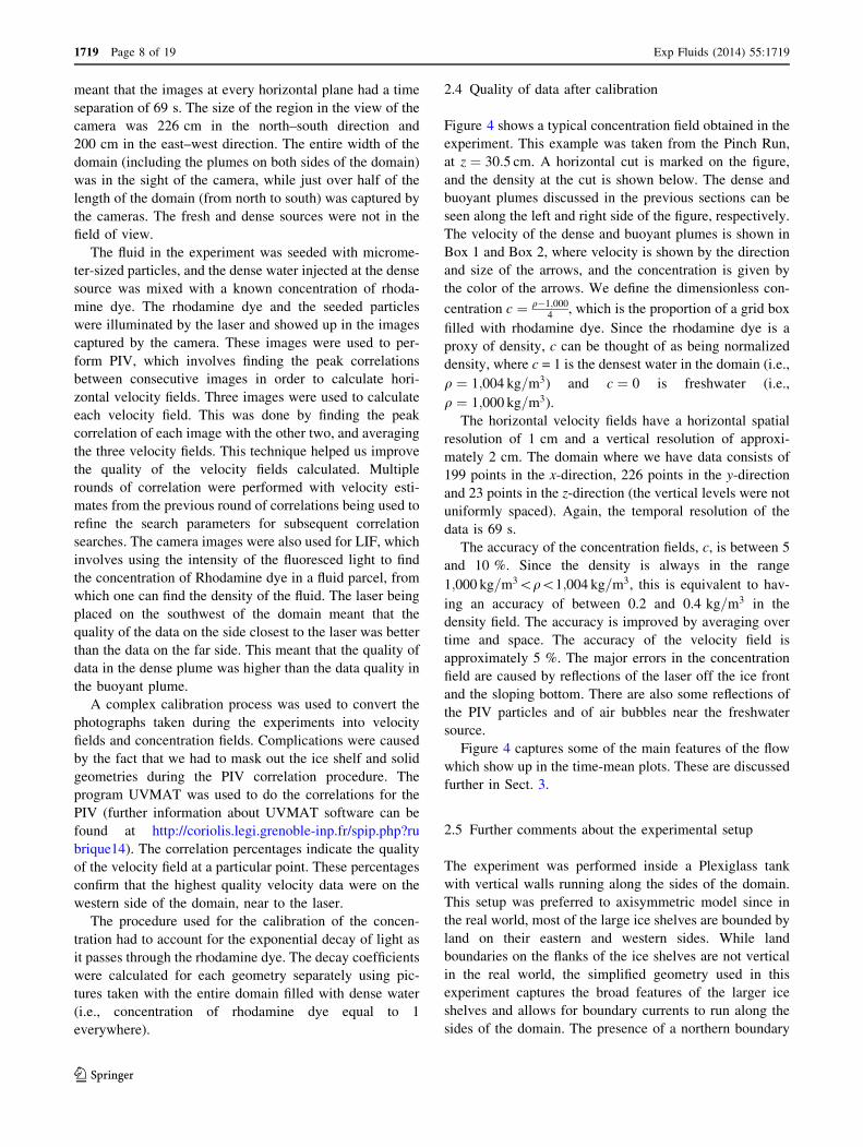
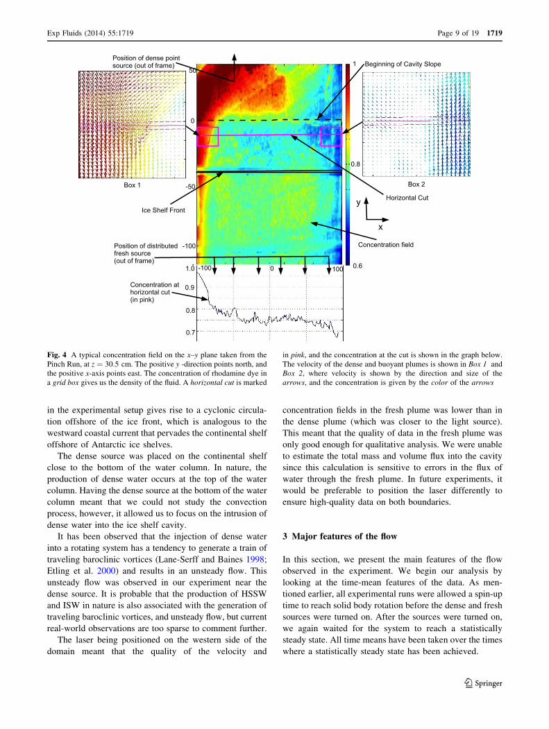
Figure 4 shows a typical concentration field obtained in the

experiment. This example was taken from the Pinch Run,

at z ¼ 30:5 cm. A horizontal cut is marked on the figure,

and the density at the cut is shown below. The dense and

buoyant plumes discussed in the previous sections can be

seen along the left and right side of the figure, respectively.

The velocity of the dense and buoyant plumes is shown in

Box 1 and Box 2, where velocity is shown by the direction

and size of the arrows, and the concentration is given by

the color of the arrows. We define the dimensionless con-

centration c ¼ q�1;0004

, which is the proportion of a grid box

filled with rhodamine dye. Since the rhodamine dye is a

proxy of density, c can be thought of as being normalized

density, where c = 1 is the densest water in the domain (i.e.,

q ¼ 1;004 kg=m3) and c ¼ 0 is freshwater (i.e.,

q ¼ 1;000 kg=m3).

The horizontal velocity fields have a horizontal spatial

resolution of 1 cm and a vertical resolution of approxi-

mately 2 cm. The domain where we have data consists of

199 points in the x-direction, 226 points in the y-direction

and 23 points in the z-direction (the vertical levels were not

uniformly spaced). Again, the temporal resolution of the

data is 69 s.

The accuracy of the concentration fields, c, is between 5

and 10 %. Since the density is always in the range

1;000 kg=m3\q\1;004 kg=m3, this is equivalent to hav-

ing an accuracy of between 0.2 and 0.4 kg=m3 in the

density field. The accuracy is improved by averaging over

time and space. The accuracy of the velocity field is

approximately 5 %. The major errors in the concentration

field are caused by reflections of the laser off the ice front

and the sloping bottom. There are also some reflections of

the PIV particles and of air bubbles near the freshwater

source.

Figure 4 captures some of the main features of the flow

which show up in the time-mean plots. These are discussed

further in Sect. 3.

2.5 Further comments about the experimental setup

The experiment was performed inside a Plexiglass tank

with vertical walls running along the sides of the domain.

This setup was preferred to axisymmetric model since in

the real world, most of the large ice shelves are bounded by

land on their eastern and western sides. While land

boundaries on the flanks of the ice shelves are not vertical

in the real world, the simplified geometry used in this

experiment captures the broad features of the larger ice

shelves and allows for boundary currents to run along the

sides of the domain. The presence of a northern boundary

1719 Page 8 of 19 Exp Fluids (2014) 55:1719

123

in the experimental setup gives rise to a cyclonic circula-

tion offshore of the ice front, which is analogous to the

westward coastal current that pervades the continental shelf

offshore of Antarctic ice shelves.

The dense source was placed on the continental shelf

close to the bottom of the water column. In nature, the

production of dense water occurs at the top of the water

column. Having the dense source at the bottom of the water

column meant that we could not study the convection

process, however, it allowed us to focus on the intrusion of

dense water into the ice shelf cavity.

It has been observed that the injection of dense water

into a rotating system has a tendency to generate a train of

traveling baroclinic vortices (Lane-Serff and Baines 1998;

Etling et al. 2000) and results in an unsteady flow. This

unsteady flow was observed in our experiment near the

dense source. It is probable that the production of HSSW

and ISW in nature is also associated with the generation of

traveling baroclinic vortices, and unsteady flow, but current

real-world observations are too sparse to comment further.

The laser being positioned on the western side of the

domain meant that the quality of the velocity and

concentration fields in the fresh plume was lower than in

the dense plume (which was closer to the light source).

This meant that the quality of data in the fresh plume was

only good enough for qualitative analysis. We were unable

to estimate the total mass and volume flux into the cavity

since this calculation is sensitive to errors in the flux of

water through the fresh plume. In future experiments, it

would be preferable to position the laser differently to

ensure high-quality data on both boundaries.

3 Major features of the flow

In this section, we present the main features of the flow

observed in the experiment. We begin our analysis by

looking at the time-mean features of the data. As men-

tioned earlier, all experimental runs were allowed a spin-up

time to reach solid body rotation before the dense and fresh

sources were turned on. After the sources were turned on,

we again waited for the system to reach a statistically

steady state. All time means have been taken over the times

where a statistically steady state has been achieved.

Fig. 4 A typical concentration field on the x–y plane taken from the

Pinch Run, at z ¼ 30:5 cm. The positive y -direction points north, and

the positive x-axis points east. The concentration of rhodamine dye in

a grid box gives us the density of the fluid. A horizontal cut is marked

in pink, and the concentration at the cut is shown in the graph below.

The velocity of the dense and buoyant plumes is shown in Box 1 and

Box 2, where velocity is shown by the direction and size of the

arrows, and the concentration is given by the color of the arrows

Exp Fluids (2014) 55:1719 Page 9 of 19 1719

123

3.1 Description of results in the Control Run

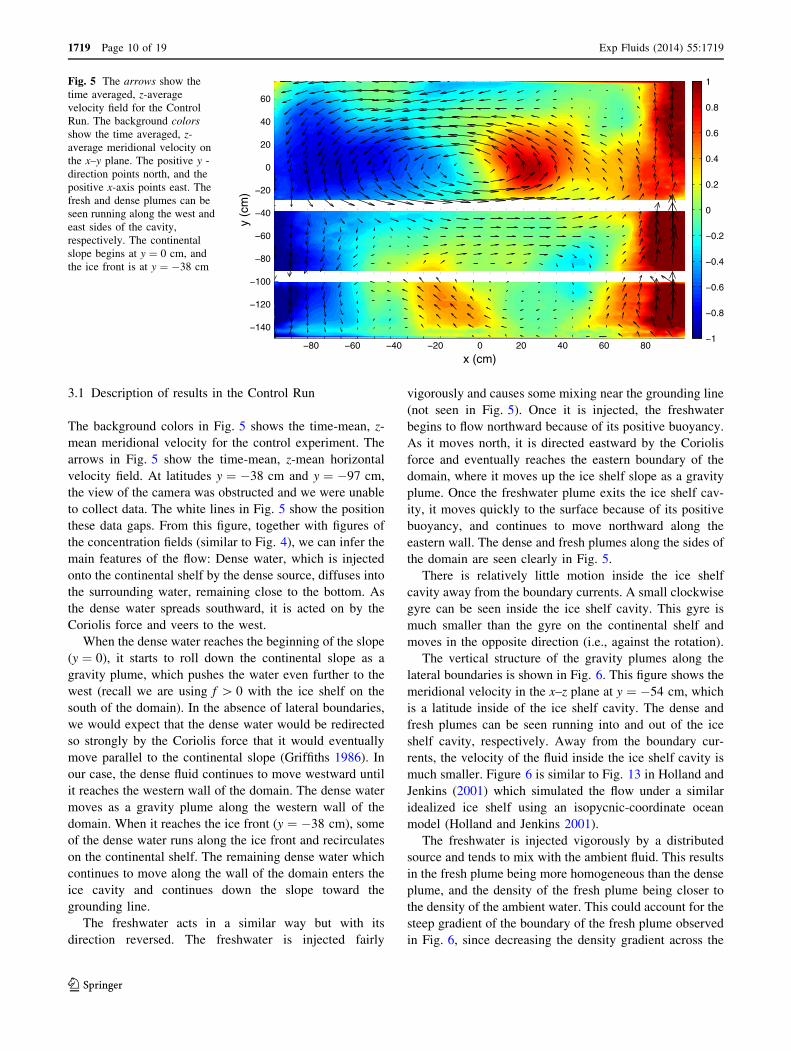
The background colors in Fig. 5 shows the time-mean, z-

mean meridional velocity for the control experiment. The

arrows in Fig. 5 show the time-mean, z-mean horizontal

velocity field. At latitudes y ¼ �38 cm and y ¼ �97 cm,

the view of the camera was obstructed and we were unable

to collect data. The white lines in Fig. 5 show the position

these data gaps. From this figure, together with figures of

the concentration fields (similar to Fig. 4), we can infer the

main features of the flow: Dense water, which is injected

onto the continental shelf by the dense source, diffuses into

the surrounding water, remaining close to the bottom. As

the dense water spreads southward, it is acted on by the

Coriolis force and veers to the west.

When the dense water reaches the beginning of the slope

(y ¼ 0), it starts to roll down the continental slope as a

gravity plume, which pushes the water even further to the

west (recall we are using f [ 0 with the ice shelf on the

south of the domain). In the absence of lateral boundaries,

we would expect that the dense water would be redirected

so strongly by the Coriolis force that it would eventually

move parallel to the continental slope (Griffiths 1986). In

our case, the dense fluid continues to move westward until

it reaches the western wall of the domain. The dense water

moves as a gravity plume along the western wall of the

domain. When it reaches the ice front (y ¼ �38 cm), some

of the dense water runs along the ice front and recirculates

on the continental shelf. The remaining dense water which

continues to move along the wall of the domain enters the

ice cavity and continues down the slope toward the

grounding line.

The freshwater acts in a similar way but with its

direction reversed. The freshwater is injected fairly

vigorously and causes some mixing near the grounding line

(not seen in Fig. 5). Once it is injected, the freshwater

begins to flow northward because of its positive buoyancy.

As it moves north, it is directed eastward by the Coriolis

force and eventually reaches the eastern boundary of the

domain, where it moves up the ice shelf slope as a gravity

plume. Once the freshwater plume exits the ice shelf cav-

ity, it moves quickly to the surface because of its positive

buoyancy, and continues to move northward along the

eastern wall. The dense and fresh plumes along the sides of

the domain are seen clearly in Fig. 5.

There is relatively little motion inside the ice shelf

cavity away from the boundary currents. A small clockwise

gyre can be seen inside the ice shelf cavity. This gyre is

much smaller than the gyre on the continental shelf and

moves in the opposite direction (i.e., against the rotation).

The vertical structure of the gravity plumes along the

lateral boundaries is shown in Fig. 6. This figure shows the

meridional velocity in the x–z plane at y ¼ �54 cm, which

is a latitude inside of the ice shelf cavity. The dense and

fresh plumes can be seen running into and out of the ice

shelf cavity, respectively. Away from the boundary cur-

rents, the velocity of the fluid inside the ice shelf cavity is

much smaller. Figure 6 is similar to Fig. 13 in Holland and

Jenkins (2001) which simulated the flow under a similar

idealized ice shelf using an isopycnic-coordinate ocean

model (Holland and Jenkins 2001).

The freshwater is injected vigorously by a distributed

source and tends to mix with the ambient fluid. This results

in the fresh plume being more homogeneous than the dense

plume, and the density of the fresh plume being closer to

the density of the ambient water. This could account for the

steep gradient of the boundary of the fresh plume observed

in Fig. 6, since decreasing the density gradient across the

−80 −60 −40 −20 0 20 40 60 80

−140

−120

−100

−80

−60

−40

−20

0

20

40

60

x (cm)

y (c

m)

−1

−0.8

−0.6

−0.4

−0.2

0

0.2

0.4

0.6

0.8

1Fig. 5 The arrows show the

time averaged, z-average

velocity field for the Control

Run. The background colors

show the time averaged, z-

average meridional velocity on

the x–y plane. The positive y -

direction points north, and the

positive x-axis points east. The

fresh and dense plumes can be

seen running along the west and

east sides of the cavity,

respectively. The continental

slope begins at y ¼ 0 cm, and

the ice front is at y ¼ �38 cm

1719 Page 10 of 19 Exp Fluids (2014) 55:1719

123

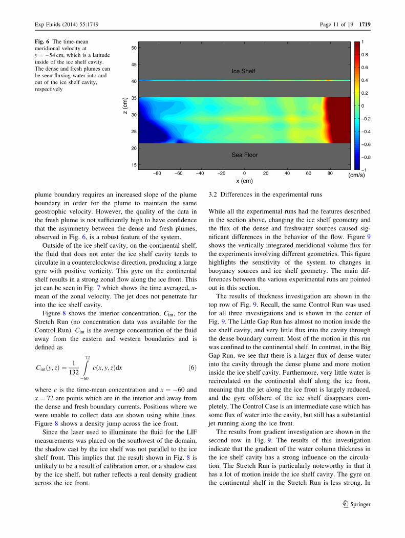
plume boundary requires an increased slope of the plume

boundary in order for the plume to maintain the same

geostrophic velocity. However, the quality of the data in

the fresh plume is not sufficiently high to have confidence

that the asymmetry between the dense and fresh plumes,

observed in Fig. 6, is a robust feature of the system.

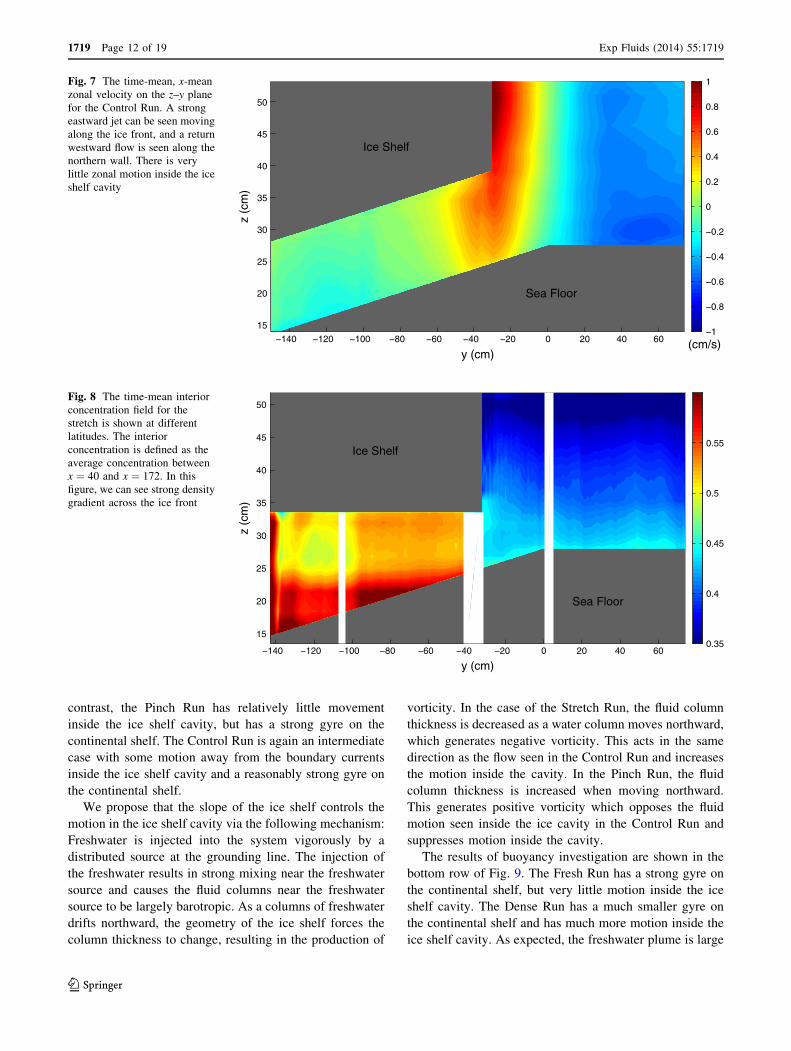
Outside of the ice shelf cavity, on the continental shelf,

the fluid that does not enter the ice shelf cavity tends to

circulate in a counterclockwise direction, producing a large

gyre with positive vorticity. This gyre on the continental

shelf results in a strong zonal flow along the ice front. This

jet can be seen in Fig. 7 which shows the time averaged, x-

mean of the zonal velocity. The jet does not penetrate far

into the ice shelf cavity.

Figure 8 shows the interior concentration, Cint, for the

Stretch Run (no concentration data was available for the

Control Run). Cint is the average concentration of the fluid

away from the eastern and western boundaries and is

defined as

Cintðy; zÞ ¼1

132

Z

72

�60

cðx; y; zÞdx ð6Þ

where c is the time-mean concentration and x ¼ �60 and

x ¼ 72 are points which are in the interior and away from

the dense and fresh boundary currents. Positions where we

were unable to collect data are shown using white lines.

Figure 8 shows a density jump across the ice front.

Since the laser used to illuminate the fluid for the LIF

measurements was placed on the southwest of the domain,

the shadow cast by the ice shelf was not parallel to the ice

shelf front. This implies that the result shown in Fig. 8 is

unlikely to be a result of calibration error, or a shadow cast

by the ice shelf, but rather reflects a real density gradient

across the ice front.

3.2 Differences in the experimental runs

While all the experimental runs had the features described

in the section above, changing the ice shelf geometry and

the flux of the dense and freshwater sources caused sig-

nificant differences in the behavior of the flow. Figure 9

shows the vertically integrated meridional volume flux for

the experiments involving different geometries. This figure

highlights the sensitivity of the system to changes in

buoyancy sources and ice shelf geometry. The main dif-

ferences between the various experimental runs are pointed

out in this section.

The results of thickness investigation are shown in the

top row of Fig. 9. Recall, the same Control Run was used

for all three investigations and is shown in the center of

Fig. 9. The Little Gap Run has almost no motion inside the

ice shelf cavity, and very little flux into the cavity through

the dense boundary current. Most of the motion in this run

was confined to the continental shelf. In contrast, in the Big

Gap Run, we see that there is a larger flux of dense water

into the cavity through the dense plume and more motion

inside the ice shelf cavity. Furthermore, very little water is

recirculated on the continental shelf along the ice front,

meaning that the jet along the ice front is largely reduced,

and the gyre offshore of the ice shelf disappears com-

pletely. The Control Case is an intermediate case which has

some flux of water into the cavity, but still has a substantial

jet running along the ice front.

The results from gradient investigation are shown in the

second row in Fig. 9. The results of this investigation

indicate that the gradient of the water column thickness in

the ice shelf cavity has a strong influence on the circula-

tion. The Stretch Run is particularly noteworthy in that it

has a lot of motion inside the ice shelf cavity. The gyre on

the continental shelf in the Stretch Run is less strong. In

x (cm)

z (c

m)

Ice Shelf

Sea Floor

(cm/s)−80 −60 −40 −20 0 20 40 60 80

15

20

25

30

35

40

45

50

−1

−0.8

−0.6

−0.4

−0.2

0

0.2

0.4

0.6

0.8

1Fig. 6 The time-mean

meridional velocity at

y ¼ �54 cm, which is a latitude

inside of the ice shelf cavity.

The dense and fresh plumes can

be seen fluxing water into and

out of the ice shelf cavity,

respectively

Exp Fluids (2014) 55:1719 Page 11 of 19 1719

123

contrast, the Pinch Run has relatively little movement

inside the ice shelf cavity, but has a strong gyre on the

continental shelf. The Control Run is again an intermediate

case with some motion away from the boundary currents

inside the ice shelf cavity and a reasonably strong gyre on

the continental shelf.

We propose that the slope of the ice shelf controls the

motion in the ice shelf cavity via the following mechanism:

Freshwater is injected into the system vigorously by a

distributed source at the grounding line. The injection of

the freshwater results in strong mixing near the freshwater

source and causes the fluid columns near the freshwater

source to be largely barotropic. As a columns of freshwater

drifts northward, the geometry of the ice shelf forces the

column thickness to change, resulting in the production of

vorticity. In the case of the Stretch Run, the fluid column

thickness is decreased as a water column moves northward,

which generates negative vorticity. This acts in the same

direction as the flow seen in the Control Run and increases

the motion inside the cavity. In the Pinch Run, the fluid

column thickness is increased when moving northward.

This generates positive vorticity which opposes the fluid

motion seen inside the ice cavity in the Control Run and

suppresses motion inside the cavity.

The results of buoyancy investigation are shown in the

bottom row of Fig. 9. The Fresh Run has a strong gyre on

the continental shelf, but very little motion inside the ice

shelf cavity. The Dense Run has a much smaller gyre on

the continental shelf and has much more motion inside the

ice shelf cavity. As expected, the freshwater plume is large

−140 −120 −100 −80 −60 −40 −20 0 20 40 60

15

20

25

30

35

40

45

50

y (cm)

z (c

m)

Ice Shelf

Sea Floor

(cm/s)−1

−0.8

−0.6

−0.4

−0.2

0

0.2

0.4

0.6

0.8

1Fig. 7 The time-mean, x-mean

zonal velocity on the z–y plane

for the Control Run. A strong

eastward jet can be seen moving

along the ice front, and a return

westward flow is seen along the

northern wall. There is very

little zonal motion inside the ice

shelf cavity

−140 −120 −100 −80 −60 −40 −20 0 20 40 60

15

20

25

30

35

40

45

50

y (cm)

z (c

m)

Ice Shelf

Sea Floor

0.35

0.4

0.45

0.5

0.55

Fig. 8 The time-mean interior

concentration field for the

stretch is shown at different

latitudes. The interior

concentration is defined as the

average concentration between

x ¼ 40 and x ¼ 172. In this

figure, we can see strong density

gradient across the ice front

1719 Page 12 of 19 Exp Fluids (2014) 55:1719

123

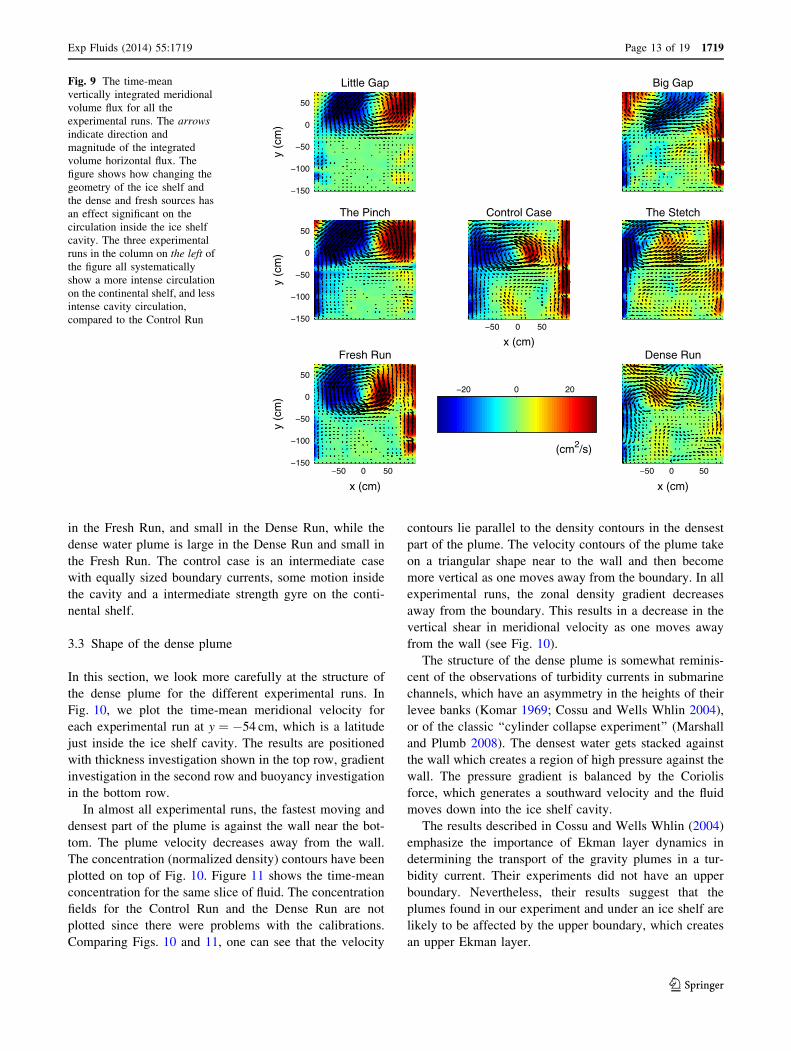
in the Fresh Run, and small in the Dense Run, while the

dense water plume is large in the Dense Run and small in

the Fresh Run. The control case is an intermediate case

with equally sized boundary currents, some motion inside

the cavity and a intermediate strength gyre on the conti-

nental shelf.

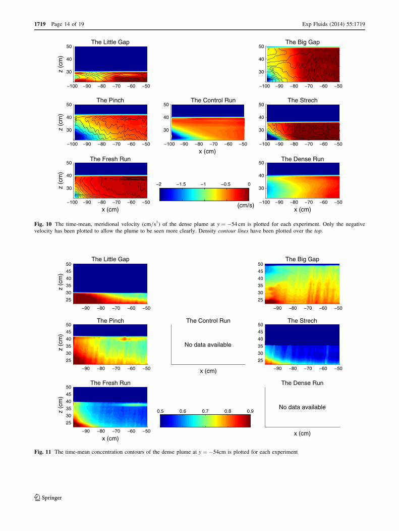
3.3 Shape of the dense plume

In this section, we look more carefully at the structure of

the dense plume for the different experimental runs. In

Fig. 10, we plot the time-mean meridional velocity for

each experimental run at y ¼ �54 cm, which is a latitude

just inside the ice shelf cavity. The results are positioned

with thickness investigation shown in the top row, gradient

investigation in the second row and buoyancy investigation

in the bottom row.

In almost all experimental runs, the fastest moving and

densest part of the plume is against the wall near the bot-

tom. The plume velocity decreases away from the wall.

The concentration (normalized density) contours have been

plotted on top of Fig. 10. Figure 11 shows the time-mean

concentration for the same slice of fluid. The concentration

fields for the Control Run and the Dense Run are not

plotted since there were problems with the calibrations.

Comparing Figs. 10 and 11, one can see that the velocity

contours lie parallel to the density contours in the densest

part of the plume. The velocity contours of the plume take

on a triangular shape near to the wall and then become

more vertical as one moves away from the boundary. In all

experimental runs, the zonal density gradient decreases

away from the boundary. This results in a decrease in the

vertical shear in meridional velocity as one moves away

from the wall (see Fig. 10).

The structure of the dense plume is somewhat reminis-

cent of the observations of turbidity currents in submarine

channels, which have an asymmetry in the heights of their

levee banks (Komar 1969; Cossu and Wells Whlin 2004),

or of the classic ‘‘cylinder collapse experiment’’ (Marshall

and Plumb 2008). The densest water gets stacked against

the wall which creates a region of high pressure against the

wall. The pressure gradient is balanced by the Coriolis

force, which generates a southward velocity and the fluid

moves down into the ice shelf cavity.

The results described in Cossu and Wells Whlin (2004)

emphasize the importance of Ekman layer dynamics in

determining the transport of the gravity plumes in a tur-

bidity current. Their experiments did not have an upper

boundary. Nevertheless, their results suggest that the

plumes found in our experiment and under an ice shelf are

likely to be affected by the upper boundary, which creates

an upper Ekman layer.

−50 0 50

x (cm)

Control Case

−150

−100

−50

0

50

y (c

m)

Little Gap Big Gap

The Stetch

−150

−100

−50

0

50

y (c

m)

The Pinch

−50 0 50−150

−100

−50

0

50

x (cm)

y (c

m)

Fresh Run

−50 0 50

x (cm)

Dense Run

(cm2/s)

−20 0 20

Fig. 9 The time-mean

vertically integrated meridional

volume flux for all the

experimental runs. The arrows

indicate direction and

magnitude of the integrated

volume horizontal flux. The

figure shows how changing the

geometry of the ice shelf and

the dense and fresh sources has

an effect significant on the

circulation inside the ice shelf

cavity. The three experimental

runs in the column on the left of

the figure all systematically

show a more intense circulation

on the continental shelf, and less

intense cavity circulation,

compared to the Control Run

Exp Fluids (2014) 55:1719 Page 13 of 19 1719

123

−100 −90 −80 −70 −60 −50

30

40

50

x (cm)

The Control Run

−100 −90 −80 −70 −60 −50

30

40

50

x (cm)

z (c

m)

The Fresh Run

−100 −90 −80 −70 −60 −50

30

40

50

x (cm)

The Dense Run

−100 −90 −80 −70 −60 −50

30

40

50

z (c

m)

The Pinch

−100 −90 −80 −70 −60 −50

30

40

50The Strech

−100 −90 −80 −70 −60 −50

30

40

50The Big Gap

−100 −90 −80 −70 −60 −50

30

40

50

z (c

m)

The Little Gap

−2 −1.5 −1 −0.5 0

(cm/s)

Fig. 10 The time-mean, meridional velocity (cm=s1) of the dense plume at y ¼ �54 cm is plotted for each experiment. Only the negative

velocity has been plotted to allow the plume to be seen more clearly. Density contour lines have been plotted over the top.

The Control Run

No data available

x (cm)

−90 −80 −70 −60 −50

25

30

35

40

45

50The Fresh Run

x (cm)

z (c

m)

The Dense Run

No data available

x (cm)

−90 −80 −70 −60 −50

25

30

35

40

45

50The Pinch

z (c

m)

−90 −80 −70 −60 −50

25

30

35

40

45

50The Strech

−90 −80 −70 −60 −50

25

30

35

40

45

50The Big Gap

−90 −80 −70 −60 −50

25

30

35

40

45

50The Little Gap

z (c

m)

0.5 0.6 0.7 0.8 0.9

Fig. 11 The time-mean concentration contours of the dense plume at y ¼ �54cm is plotted for each experiment

1719 Page 14 of 19 Exp Fluids (2014) 55:1719

123

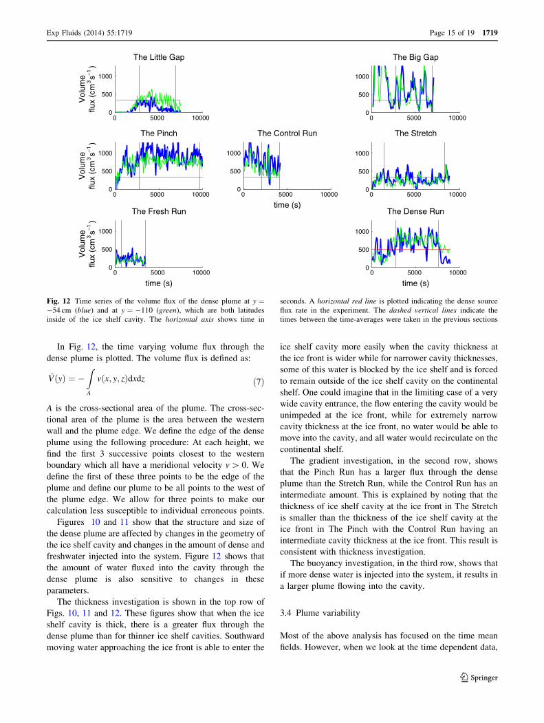
In Fig. 12, the time varying volume flux through the

dense plume is plotted. The volume flux is defined as:

VðyÞ ¼ �Z

A

vðx; y; zÞdxdz ð7Þ

A is the cross-sectional area of the plume. The cross-sec-

tional area of the plume is the area between the western

wall and the plume edge. We define the edge of the dense

plume using the following procedure: At each height, we

find the first 3 successive points closest to the western

boundary which all have a meridional velocity v [ 0. We

define the first of these three points to be the edge of the

plume and define our plume to be all points to the west of

the plume edge. We allow for three points to make our

calculation less susceptible to individual erroneous points.

Figures 10 and 11 show that the structure and size of

the dense plume are affected by changes in the geometry of

the ice shelf cavity and changes in the amount of dense and

freshwater injected into the system. Figure 12 shows that

the amount of water fluxed into the cavity through the

dense plume is also sensitive to changes in these

parameters.

The thickness investigation is shown in the top row of

Figs. 10, 11 and 12. These figures show that when the ice

shelf cavity is thick, there is a greater flux through the

dense plume than for thinner ice shelf cavities. Southward

moving water approaching the ice front is able to enter the

ice shelf cavity more easily when the cavity thickness at

the ice front is wider while for narrower cavity thicknesses,

some of this water is blocked by the ice shelf and is forced

to remain outside of the ice shelf cavity on the continental

shelf. One could imagine that in the limiting case of a very

wide cavity entrance, the flow entering the cavity would be

unimpeded at the ice front, while for extremely narrow

cavity thickness at the ice front, no water would be able to

move into the cavity, and all water would recirculate on the

continental shelf.

The gradient investigation, in the second row, shows

that the Pinch Run has a larger flux through the dense

plume than the Stretch Run, while the Control Run has an

intermediate amount. This is explained by noting that the

thickness of ice shelf cavity at the ice front in The Stretch

is smaller than the thickness of the ice shelf cavity at the

ice front in The Pinch with the Control Run having an

intermediate cavity thickness at the ice front. This result is

consistent with thickness investigation.

The buoyancy investigation, in the third row, shows that

if more dense water is injected into the system, it results in

a larger plume flowing into the cavity.

3.4 Plume variability

Most of the above analysis has focused on the time mean

fields. However, when we look at the time dependent data,

0 5000 100000

500

1000

time (s)

The Control Run

0 5000 100000

500

1000

time (s)

The Fresh Run

0 5000 100000

500

1000

time (s)

The Dense Run

0 5000 100000

500

1000

The Pinch

0 5000 100000

500

1000

The Stretch

0 5000 100000

500

1000

The Big Gap

0 5000 100000

500

1000

flux

(cm

3s−

1)

The Little Gap

Vol

ume

flux

(cm

3s−

1)

Vol

ume

flux

(cm

3s−

1)

Vol

ume

Fig. 12 Time series of the volume flux of the dense plume at y ¼�54 cm (blue) and at y ¼ �110 (green), which are both latitudes

inside of the ice shelf cavity. The horizontal axis shows time in

seconds. A horizontal red line is plotted indicating the dense source

flux rate in the experiment. The dashed vertical lines indicate the

times between the time-averages were taken in the previous sections

Exp Fluids (2014) 55:1719 Page 15 of 19 1719

123

we see that the circulation inside the cavity and the flow

through the plumes are in fact highly variable. In this

section, we focus on the time dependence of the flow in the

dense plume.

Figure 12 shows a time series of the volume flux of the

dense plume (defined above) at y ¼ �54 (blue) and at y ¼�110 (green), which are both latitudes inside of the ice

shelf cavity. A horizontal red line is plotted indicating the

flux of water at the dense source in the experiment. The

flux at the two latitudes varies together since the time scale

of the oscillations is much longer than the time taken for

fluid to move down the plume from the northern latitude to

the southern latitude.

The most striking feature in Fig. 12 is that the various

experimental runs have different volume fluxes through the

dense plume and that these volume fluxes are highly var-

iable. The variabilities in the various experimental runs

have different amplitudes and different periods depending

on the geometry of the ice shelves and buoyancy sources

used. As discussed in the previous section, the amplitude of

volume flux through the plume is proportional to the

thickness of the opening of the ice shelf cavity at the ice

front.

In thickness investigation (top row of Fig. 12), we see

that the plume is more variable for a thick ice shelf cavity

than for the thin cavity. For the thick ice shelf, the

amplitude of the variations is largest, and the period of

the variations is longest. In gradient investigation (second

row in Fig. 12), we see that period of the oscillations in

the plume in the Stretch Run is larger than in the Pinch

Run, with the Control Run having an intermediate period.

The amplitude of the oscillations also appears to be larger

in the Stretch Run. This is especially apparent when the

time series is normalized. In the buoyancy investigation

(bottom row of Fig. 12), we see that amplitude and period

of the oscillations are larger and longer for the Dense Run

than for the Fresh Run with the Control Run being

intermediate.

The variability of the plume seems to indicate how

much the circulation inside the ice shelf cavity is influ-

enced by the variability outside of the cavity. The experi-

mental runs with strong dynamic barrier at the ice front

have restricted movement inside the ice shelf cavity, and

limited variability inside the plume. The runs which have a

weaker dynamic barrier at the ice front have more motion

inside the ice shelf cavity, and have a more variable dense

plume.

Looking carefully at the time varying data, we see that

the dense water does not move smoothly from the source to

the plume, but instead arrives in pulses. These pulses cause

the oscillations in the flow rate seen in Fig. 12. The fluid is

injected smoothly into the domain by the dense source (i.e.,

without pulses), which implies that some other mechanism

is causing the flow to be unsteady. The most likely can-

didates are baroclinic instability of the gyre on the conti-

nental shelf and that eddies are created at the dense source

when the dense fluid is released into the domain.

4 Discussion

In the previous sections, we saw evidence of the dynamic

significance of the ice front in largely blocking water from

entering and exiting the ice shelf cavity and that this

blocking effect was significantly altered by changing the

ice geometry and buoyancy fluxes. We discuss these in

turn:

The blocking effect of the ice shelf front has been noted

by other authors using numerical models (Determan and

Gerdes 1994; Grosfeld et al. 1997). Grosfeld et al. (1997)

used a three-dimensional numerical model and observed

that the flow was dominated by the barotropic mode, which

steers the flow along the ice front rather than into the ice

shelf cavity. The presence of the ice shelf imposes a change

in water column thickness which presents a barrier for the

barotropic flow. The barotropic flow tends to move along fH

contours which run parallel to the shelf. For this reason, the

zonal jet outside the ice shelf cavity runs along the ice front

but does not enter.

However, while the results presented above do demon-

strate the blocking effect of the ice shelf, they also dem-

onstrate that this blocking effect is not as severe as

previously suggested (Determan and Gerdes 1994; Gros-

feld et al. 1997). Figure 7 show that although the jet runs

along the ice front, it does leak into the ice shelf cavity to

some extent. There is a significant vertical shear in the

velocity of the jet along the ice front. This indicates that the

jet is not solely dominated by the barotropic mode. The

leaking of the jet into the cavity may be a result of baro-

clinic instability. Furthermore, Fig. 5 shows there is some

flux into and out of the ice shelf cavity away from the

boundary currents, despite the dynamic barrier imposed by

the ice shelf.

Furthermore, water is able to flux into and out of the

cavity relatively freely through the dense and fresh plumes.

This is because in the dense and fresh plumes, the strati-

fication decouples the water column and the plumes are

able to enter/exit the ice shelf cavity more easily (Holland

and Jenkins 2001).

The results from thickness investigation, gradient

investigation and buoyancy investigation indicate that the

blocking effect of the ice shelf front, the amount of

movement inside the ice shelf cavity and the flux of water

through the density plumes are strongly affected by the

geometry of the ice shelf cavity, and the amount of dense

and freshwater injected into the system. Figure 13 is a

1719 Page 16 of 19 Exp Fluids (2014) 55:1719

123

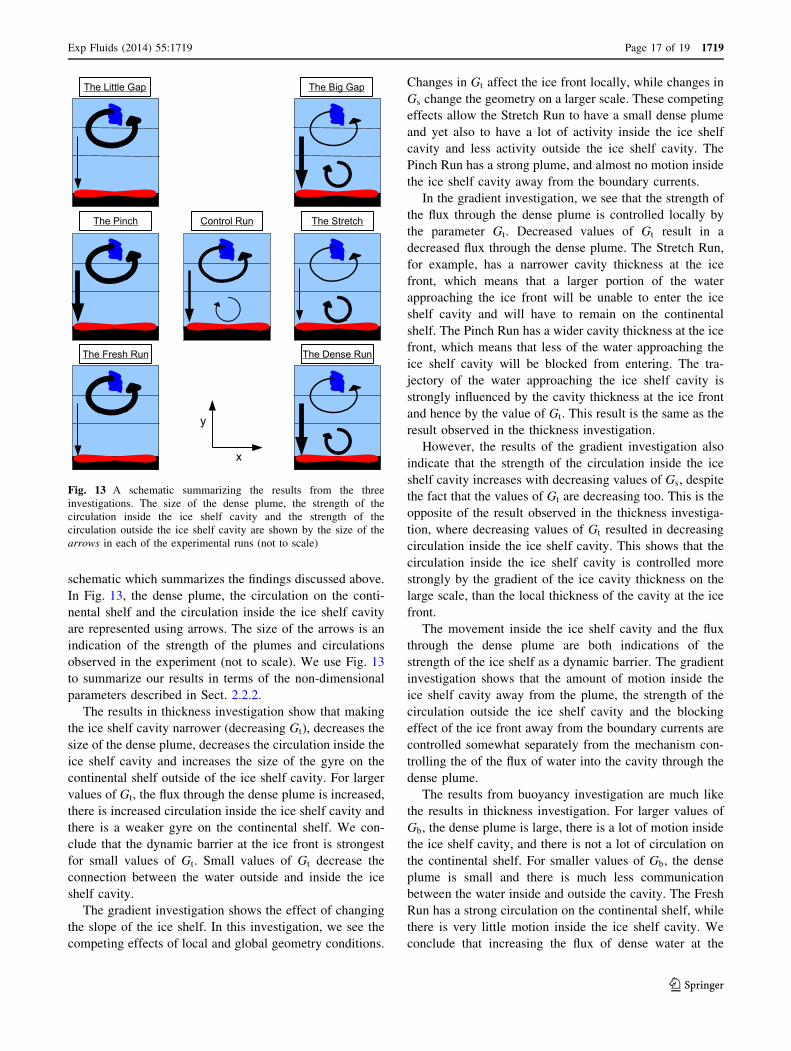
schematic which summarizes the findings discussed above.

In Fig. 13, the dense plume, the circulation on the conti-

nental shelf and the circulation inside the ice shelf cavity

are represented using arrows. The size of the arrows is an

indication of the strength of the plumes and circulations

observed in the experiment (not to scale). We use Fig. 13

to summarize our results in terms of the non-dimensional

parameters described in Sect. 2.2.2.

The results in thickness investigation show that making

the ice shelf cavity narrower (decreasing Gt), decreases the

size of the dense plume, decreases the circulation inside the

ice shelf cavity and increases the size of the gyre on the

continental shelf outside of the ice shelf cavity. For larger

values of Gt, the flux through the dense plume is increased,

there is increased circulation inside the ice shelf cavity and

there is a weaker gyre on the continental shelf. We con-

clude that the dynamic barrier at the ice front is strongest

for small values of Gt. Small values of Gt decrease the

connection between the water outside and inside the ice

shelf cavity.

The gradient investigation shows the effect of changing

the slope of the ice shelf. In this investigation, we see the

competing effects of local and global geometry conditions.

Changes in Gt affect the ice front locally, while changes in

Gs change the geometry on a larger scale. These competing

effects allow the Stretch Run to have a small dense plume

and yet also to have a lot of activity inside the ice shelf

cavity and less activity outside the ice shelf cavity. The

Pinch Run has a strong plume, and almost no motion inside

the ice shelf cavity away from the boundary currents.

In the gradient investigation, we see that the strength of

the flux through the dense plume is controlled locally by

the parameter Gt. Decreased values of Gt result in a

decreased flux through the dense plume. The Stretch Run,

for example, has a narrower cavity thickness at the ice

front, which means that a larger portion of the water

approaching the ice front will be unable to enter the ice

shelf cavity and will have to remain on the continental

shelf. The Pinch Run has a wider cavity thickness at the ice

front, which means that less of the water approaching the

ice shelf cavity will be blocked from entering. The tra-

jectory of the water approaching the ice shelf cavity is

strongly influenced by the cavity thickness at the ice front

and hence by the value of Gt. This result is the same as the

result observed in the thickness investigation.

However, the results of the gradient investigation also

indicate that the strength of the circulation inside the ice

shelf cavity increases with decreasing values of Gs, despite

the fact that the values of Gt are decreasing too. This is the

opposite of the result observed in the thickness investiga-

tion, where decreasing values of Gt resulted in decreasing

circulation inside the ice shelf cavity. This shows that the

circulation inside the ice shelf cavity is controlled more

strongly by the gradient of the ice cavity thickness on the

large scale, than the local thickness of the cavity at the ice

front.

The movement inside the ice shelf cavity and the flux

through the dense plume are both indications of the

strength of the ice shelf as a dynamic barrier. The gradient

investigation shows that the amount of motion inside the

ice shelf cavity away from the plume, the strength of the

circulation outside the ice shelf cavity and the blocking

effect of the ice front away from the boundary currents are

controlled somewhat separately from the mechanism con-

trolling the of the flux of water into the cavity through the

dense plume.

The results from buoyancy investigation are much like

the results in thickness investigation. For larger values of

Gb, the dense plume is large, there is a lot of motion inside

the ice shelf cavity, and there is not a lot of circulation on

the continental shelf. For smaller values of Gb, the dense

plume is small and there is much less communication

between the water inside and outside the cavity. The Fresh

Run has a strong circulation on the continental shelf, while

there is very little motion inside the ice shelf cavity. We

conclude that increasing the flux of dense water at the

Fig. 13 A schematic summarizing the results from the three

investigations. The size of the dense plume, the strength of the

circulation inside the ice shelf cavity and the strength of the

circulation outside the ice shelf cavity are shown by the size of the

arrows in each of the experimental runs (not to scale)

Exp Fluids (2014) 55:1719 Page 17 of 19 1719

123

dense source (increasing Gb) has the effect of decreasing

the dynamical barrier at the ice front which results in a

stronger connection between the motion inside the ice shelf

cavity and the motion on the continental shelf. Decreasing

Gb results in a strengthening of the dynamical barrier at the

ice front, and decreases the connection between the cir-

culation inside of the ice shelf cavity and the circulation on

the continental shelf.

5 Conclusion

A laboratory experiment has been set up to simulate the

density-driven currents under ice shelves. The density

current was forced by the input of dense water on the

continental shelf and freshwater at the grounding line. The

central question asked was how water of different densities

is able to enter and exit the ice shelf cavity and whether its

ability to enter the ice shelf cavity is affected by the

geometry of the ice shelf, and the strength of the dense and

freshwater sources. This question has important scientific

significance since the flux of dense water into the ice shelf

cavity ultimately impacts the melt rates of the ice shelves.

From the results presented above, we draw three con-

clusions. Firstly, the results show that the movement in and

out of the ice shelf cavity is largely restricted away from

the boundary currents. In this sense, the ice shelf front acts

as a dynamical barrier restricting the connection between

the water inside the ice shelf cavity and the water outside

the ice shelf cavity. The dynamic barrier imposed by the

ice front was observed to be present for various ice shelf

geometries. However, the dynamical barrier was not as

strong as previously argued (Determan and Gerdes 1994;

Grosfeld et al. 1997), and some water was able to pass

through the ice front away from the boundary currents.

Our second finding was that fluid was able to enter and

exit the ice shelf cavity very easily through the dense and

fresh plumes running along the boundaries of the domain.

These boundary currents take on a triangular shape with

density contours lying parallel to velocity contours. The

boundary currents transport water in and out of the ice shelf

cavity very efficiently. This suggests that real-world ice

shelf cavity boundary currents are very efficient at trans-

porting warm, salty water into the ice shelf cavity, and that

warm, salty water arriving on the continental shelf will

likely be fluxed into the cavity despite the dynamic barrier

imposed at the ice shelf front.

The third finding is that changes to the ice shelf

geometry and changes to the source strength of the dense

and freshwater sources were shown to have a significant

effect on the time mean circulation under the ice shelf.

The thickness of the ice shelf cavity at the ice front was

shown to be an important parameter in setting the volume

flux through the dense plume. The thickness of the ice

shelf cavity and the slope of the ice shelf were shown to

have a strong influence on the strength of the circulation

inside the ice shelf cavity. Ice shelves whose thickness

decreases as one moves from the grounding line toward

the ice front were shown to have more motion inside the

ice shelf cavity. Furthermore, it was shown that increasing

the strength of the dense source resulted in an increase in

the amount of motion inside the ice shelf cavity, and a

weakening of the dynamical barrier imposed by the ice

front.

The experiments described here are a first attempt at

using laboratory experiments to mimic ice shelf circula-

tion. We were able to simulate the circulation under the ice

shelf and generate a flow with the same broad features as

the circulation surmised under real-world ice shelves using

limited data. The experimental results presented above

show that the circulation inside the ice shelf cavity and the

effectiveness of the ice front as a dynamical barrier are

both sensitive to the changes in the buoyancy sources and

the ice shelf geometry.

Acknowledgments A. Stern and D, Holland were supported from

NSF grants ANT-1144504 and ANT-0732869, both from the Ant-

arctic Integrated System Science (AISS) program of the USA

National Science Foundation (NSF), as well as the Center for Sea

Level Change (CSLC) of New York University Abu Dhabi Grant

G1204. The technical assistance of Henri Didelle and Samuel Viboud

is highly valued. The experimental campaign was supported by the

European Community’s Sixth Framework Programme through the

Integrated Infrastructure Initiative HYDRALAB III, Contract no.

022441 (RII3).

References

Adrian RJ (2005) Twenty years of particle image velocimetry. Exp

Fluids 39(2):159–169

Arthun M, Nicholls KW, Boehme L (2013) Wintertime water mass

modification near an antarctic ice front. J Phys Oceanogr

43:359–365. doi:10.1175/JPO-D-12-0186.1

Assmann K, Hellmer H, Beckmann A (2003) Seasonal variation in

circulation and water mass distribution on the Ross Sea

continental shelf. Antarct Sci 15(1):3–11. doi:10.1017/

S0954102003001007

Cenedese C, Whitehead JA, Ascarelli TA, Ohiwa M (2004) A dense

current flowing down a sloping bottom in a rotating fluid. J Phys

Oceanogr 34:188–203

Conway H, Hall BL, Denton GH, Gades AM, Waddington ED (1999)

Past and future grounding-line retreat of the West Antarctic ice

sheet. Science 286(5438):280–283

Cossu R, Wells Whlin MG (2004) Influence of the Coriolis force on

the velocity structure of gravity currents in straight submarine

channel systems. J Geophys Res 115:C11016. doi:10.1029/

2010JC006208

Davey FJ (2004) Ross Sea Bathymetry. In: Institute of Geological and

Nuclear Sciences Geophysical Map 16, scale 1:2,000,000,

Version 1.0., Institute of Geology and Nuclear Sciences, Lower

Hutt, New Zealand

1719 Page 18 of 19 Exp Fluids (2014) 55:1719

123

Determan J, Gerdes R (1994) Melting and freezing beneath ice

shelves: implications from a three-dimensional ocean-circulation

model. Ann Glaciol 20:413–419

Etling D, Gelhardt F, Schrader U, Brennecke F, Kuhn G, Chabert

dHieres G, Didelle H (2000) Experiments with density currents

on a sloping bottom in a rotating fluid. Dyn Atmos Oceans

31:139–164

Foldvik A, Gammelsrød T, Nygaard E, Osterhus S (1983) Current

measurements near Ronne Ice Shelf: implications for circulation

and melting. J Geophys Res 106:4463–4477

Gordon AL, Orsi AH, Muench R, Huber BA, Zambianchi E, Visbeck

M (2009) Western Ross Sea continental slope gravity currents.

Deep-Sea Res. Part II 56(796–817):20. doi:10.1016/j.dsr2.2008.

10.037

Greenspan HP, Howard LN (1963) On a time-dependent motion of a

rotating fluid. J Fluid Mech 17:385

Griffiths RW, Hopfinger EJ (1983) Gravity currents moving along a

lateral boundary in a rotating frame. J Fluid Mech 134:357–399

Griffiths RW (1986) Gravity currents in rotating systems. Ann Rev

Fluid Mech 18:59–89

Grosfeld K, Gerdes R, Determann J (1997) Thermohaline circulation

and interaction between ice shelf cavities and the adjacent open

ocean. J Geophys Res 102(C7):15595–15610. doi:10.1029/

97JC00891

Hattermann T, Nøst AK, Lilly JM, Smedsrud JM (2012) Two years of

oceanic observations below the Fimbul Ice Shelf, Antarctica.

Geophys Res Lett 39(L12605):1–6. doi:10.1029/2012GL051012

Hellmer HH, Olbers DJ (1989) A two-dimensional model for the

thermohaline circulation under an ice shelf. Antarct Sci

1:325–336

Holland DM, Jenkins A (1999) Modeling thermodynamic iceocean

interactions at the base of an ice shelf. J Phys Oceanogr

29:1787–1800

Holland DM, Jenkins A (2001) Adaptation of an isopycnic coordinate

ocean model for the study of circulation beneath ice shelves.

Mon Wea Rev 129:1905–1927

Holland PR, Feltham DL (2006) The effects of rotation and ice shelf

topography on frazil-laden Ice Shelf Water plumes. J Phys

Oceanogr 36:2312–2327

Holman JP (2002) Heat transfer. McGraw-Hill, New York

Houcine I, Vivier H, Plasari E, David R, Villermaux J (1996) Planar

laser induced fluorescence technique for measurements of

concentration fields in continuous stirred tank reactors. Exp

Fluids 22(2):95–102

Jenkins A (1991) A one-dimensional model of ice shelf-ocean

interaction. J Geophys Res Oceans 96(C11):20671–20677

Jenkins A, Dutrieux P, Jacobs S, McPhail S, Perrett J, Webb A, White

D (2012) Autonomous underwater vehicle exploration of the

ocean cavity beneath an Antarctic ice shelf. Oceanography

25(3):202–203. doi:10.5670/oceanog.2012.95

Killworth OD, Paldor N, Stern ME (1984) Wave propagation and

growth on a surface front in a two-layer geostrophic current.

J Marine Res 42:761–785

Komar PD (1969) The channelized flow of turbidity currents with

application to Monterey deep-sea fan channel. J Geophys Res

74:4544–4558. doi:10.1029/JC074i018p04544

Lane-Serff G, Baines P (1998) Eddy formation by dense flows on

slopes in a rotating fluid. J Fluid Mech 363:229–252

MacAyeal DR (1984) Thermohaline circulation below the Ross ice

shelf: a consequence of tidally induced vertical mixing and basal

melting. J Geophys Res 89:597–606

MacAyeal DR (1985) Evolution of tidally triggered meltwater plumes

below ice shelves. In: Jacobs SS (ed) Oceanology of the antarctic

continental shelf. American Geophysical Union, Washington

Makinson K, Schrder M, Østerhus S (2006) Effect of critical latitude

and seasonal stratification on tidal current profiles along Ronne

Ice Front, Antarctica. J Geophys Res 111:C03022. doi:10.1029/

2005JC003062

Makinson K, Schroder M, Østerhus S (2005) Seasonal stratification

and tidal current profiles along Ronne Ice Front. Frisp, Report 16

Marshall J, Plumb RA (2008) Atmosphere, ocean and climate dynamics:

an introductory text, vol 93. Academic Press, pp 123–128

Mathiot P, Jourdain NC, Barnier B, Galle B, Molines JM, Le Sommer

J, Penduff T (2012) Sensitivity of coastal polynyas and high-

salinity shelf water production in the Ross Sea, Antarctica, to the

atmospheric forcing. Ocean Dyn 62:701–723. doi:10.1007/

s10236-012-0531-y

Millero FJ (1978) Freezing point of sea water: Eighth report of the

Joint Panel of Oceanographic Tables and Standards. Appendix 6

UNESCO Tech Pap Mar Sci 28:29–31

Nicholls KW (1996) Temperature variability beneath Ronne Ice

Shelf, Antarctica, from thermistor cables. J Phys Oceanogr

11:1199–1210

Nicholls KW, Padman L, Schroder M, Woodgate RA, Jenkins A,

Østerhus S (2003) Water mass modification over the continental

shelf north of Ronne Ice Shelf, Antarctica. J Geophys Res

108(C8):3260. doi:10.1029/2002JC001713

Nicholls KW, Osterhus S, Makinson K (2009) Ice-Ocean processes

over the continental shelf of the southern Weddell Sea,

Antarctica: a review. Rev Geophys 47:RG3003. doi:10.1029/

2007RG000250

Nunez-Riboni I, Fahrbach E (2010) An observation of the banded

structure of the Antarctic Coastal Current at the prime meridian.

Polar Res 29:322–329

Orsi AH, Smethie WM Jr, Bullister JL (2002) On the total input of

Antarctic waters to the deep ocean: a preliminary estimate from

chlorofluorocarbon measurements. J Geophys Res 107(C8).

doi:10.1029/2001JC000976

Stern ME, Whitehead JA, Hua BL (1982) The intrusion of a density

current along the coast of a rotating fluid. J Fluid Mech

123:237–266

Stern AA, Dinniman MS, Zagorodnov V, Tyler SW, Holland DM

(2013) Intrusion of warm surface water beneath the McMurdo

Ice Shelf, Antarctica. J Geophys Res Oceans 118:7036–7048.

doi:10.1002/2013JC008842Wahlin AK, Darelius E, Cenedese C, Lane-Serff GF (2008)

Laboratory observations of enhanced entrainment in dense

overflows in the presence of submarine canyons and ridges.

Deep-sea Res 1(55):737–750. doi:10.1016/J.DSR.2008.02.007

Zatsepin AG, Didkovski VL, Semenov AV (1996) A self-oscillatory

mechanism of inducing a vortex sloping bottom in a rotating

fluid. Oceanology 38:43–50

Exp Fluids (2014) 55:1719 Page 19 of 19 1719

123