„ .\U

Ö:. I V

THE EFFECT OF BALL MILL OPERATING PARAMETERS ON MINERALLIBERATION

by

Hector E. Rojas

Dissertation submitted to the Faculty of theVirginia Polytechnic Institute and State University

in partial fulfillment of the requirements for the degree of

Masters of Science

in

Mining and Minerals Engineering

APPROVED:

G. T. Adel, Chairman

I

R. E./Yoon ‘J

4 G. HC Luttrell

Karmis

November, 1989

Blacksburg, Virginia

THE EFFECT OF BALL MILL PARAMETERS ON MINERAL LIBERATION

Hector E. Rojas

Committee Chairman: Dr. G.T. AdelMining and Mineral Engineering

(ABSTRACT)

In previous studies, the analysis of ball mill

° operating parameters and their effects on breakage phenomena

has been limited to homogeneous materials. Though theseß

studies have proven to be an asset in predictions of product

size distributions and mill scale—up, they have not

addressed the primary role of grinding, i.e. liberation.I

The present investigation analyzes the effect of ball

U mill operating· parameters on the breakage rates of both

t· liberated and composite material. The operating parameters

studied include mill rotational speed, ball size, millI

charge and wet versus dry grinding. Breakage rates have been

determined experimentally utilizing a SEM—IPS image

analyzer. The mineral sample used was acquired from ASARCO's

Young Mine which is located in Jefferson City Tennessee. It

was a binary ore consisting of sphalerite and dolomite.

Batch grinding experiments were conducted to provide

breakage rates for the various composition classes.

Breakage rates were then normalized with respect to energy

to see if the changes in breakage rates associated with mill

operating parameters were due to changes in breakage

kinetics, or simply a function of energy input.

The energy normalized data indicates that the free

dolomite breakage rates tend to normalize with respect to

»energy in the case of varying interstitial fillings.

Furthermore, changes in mill rotational speed tend to

provide energy normalizable breakage rates for· both free

dolomite and sphalerite. In all other cases, analysis of

the breakage rates and energy specific breakage rates

indicate that a change in breakage kinetics may be

occurring.'

In general, particles containing a high proportion of

sphalerite are more apt to break under impact conditions. On

the other hand, particles containing a large proportion of

dolomite were found to prefer attrition breakage conditions.

ACKNOWLEDGEMENT

The author wishes to express his appreciation for the

support and encouragement provided by his advisor, Dr. G. T.

Adel as well as the rest of the faculty at Virginia Tech.

Their interest and involvement with this project made the

time and effort a worthwhile experience. Special thanks are

due to ASARCO for continuing its cooperation with Virginia

Tech in providing mineral ore samples from its Young Mine

operation.

This research has been supported by the Department of

the Interior's Mineral Institute program administered by the

Bureau of Mines through the Generic Mineral Technology

Center for Comminution under grant # G1125149. The author

wishes to extend his ;ppr§c1a:1¤¤ for this support as well

as that provided by Dr. M. E. Karmis and the Department of

Mining and Minerals Engineering for providing the author

with tuition scholarships. °

Recognition should be given to Roy Hill for performing

the chemical assays as well as technical assistance with the

scanning electron microscope. Special thanks are extended to

Bloice Davison, Brian Robinette and Hillary Smith for their

help in sample preparation and polishing. Sincere gratitude

is also extended to the numerous friendships that have been

nurtured throughout the years at Virginia Tech with fellow

graduate students, in particular those of Woo Zin Choi,

Richard Forrest, Margie Lagno, Van Davis, Jennifer Smith,

Michael Stallard, Joseph Zachwieja and Jorge Yordan.

The author wishes to express special acknowledgement to

the loving support of his parents Their encouragement and

devotion made it all possible. As a third generation

Mining Engineer, the author wishes to dedicate this

thesis

whose exemplary career influenced the choice of this

profession.

4 TABLE OF CONTENTS

PAGE

ABSTRACT

ACKNOWLEDGMENT ........................................ iv

TABLE OF CONTENTS ..................................... vi

LIST OF FIGURES ....................................... ix

LIST OF TABLES ........................................ xi

I. INTRODUCTION ..................................... 1

1.1 Statement of Proble ......................... 1

1.2 Literature Review ............................. 3

1.2.1 Grinding Theories and Models .......... 3

a. Grinding Theories .................... 3

b. Population Balance Models ............ 6

1.2.2 - Liberation Theory and Models ......4.... 9

a. Degree of Liberation ................. 9

b. Liberation Modeling ...................10

1.2.3 Quantification of Mineral Liberation ...14

a. Image Analysis Techniques .............14

b. Volumetric Approximation Techniques ...15A

1.2.4 Effect of Mill Parameter Changes on ....17Homogeneous Grinding

1.3 Research Objectives........................... 26 _l'

II. EXPERIMENTAL PROCEDURE ........................... 28

2.1 Ore Sample ................................... 28

2.2 Grinding and Torque Sensing Equipment ........ 29 ·“vi

‘

2.3 Sizing Equipment ............................. 29

2.4 SEM-IPS Image Analyzer ....................... 30

2.5 Experimental Procedure ....................... 33

2.5.1 Sample Preparation ..................... 33

2.5.2 Grinding Experiments ................... 34

2.5.3 Briquetting and Polishing .............. 35I

2.5.4 Liberation Analysis .................... 36

2.5.5 Statistical Analysis ................... 39

III. EXPERIMENTAL RESULTS ............................. 42

3.1 Comparison of Image Analysis to Chemical Assays 42

3.2 Feed Characterization for Mono—Sized Feeds .....43

3.3 Determination of Breakage Rates ................45

3.4 Determination ef Energy Specific Breakage ..... 48Rates

3.5 Effect of Image Analysis Error on Breakage .... 49Rate Calculations

IV. DISCUSSION OF RESULTS ..............................52

4.1 Analysis of Breakage Rates .....................52

4.2 Analysis of Energy Specific Breakage Rates .....58

4.3 Comparison of Results to Previous Studies ......65

V. SUMMARY AND CONCLUSIONS ............................72

VI. SUGGESTIONS FOR FUTURE WORK ........................76

REFERENCES79

APPENDIX I: Image Analysis Data..........................84l

APPENDIX II: Percent Remaining Values fortheDisappearancePlots ........................90

APPENDIX III: Disappearance Plots .......................96

APPENDIX IV: Breakage and Energy Specific -.......I.......107Breakage Rates ~ _ ‘

V ' vii _

APPENDIX V: Chemical Assay Prccedure ...................110

VITA ...................................................112

V _ I ' viii l l

LIST OF FIGURESPage

Figure 2.1 SEM-IPS image analyzer .................... 31

Figure 2.2 Image Processing Procedures ................ 37 _

Figure 3.1 Example of a 14x20 mesh feed .............. 44· distribution for a 40% critical speed

test

Figure 3.2 Example of a disappearance plot for ....... 4714x20 mesh feed at 40% critial speed

Figure 4.1 Breakage rate versus percent .............. 53sphalerite plots for different millrotational speeds with 14x2O mesh- feed

Figure 4.2 Breakage rate versus percent .............. 55sphalerite for various ball sizediameters with 10x14 mesh feed

Figure 4.3 Breakage rate versus percent .............. 57sphalerite for various interstitialfilling with 10x14 mesh feed

Figure 4.4 Breakage rate versus percent .............. 59sphalerite for dry and 70 percentsolids grinding environments with14x20 mesh feed

Figure 4.5 Energy normalized breakage rates .......... 61versus percent sphalerite fordifferent mill rotational speedswith 14x20 mesh feed

Figure 4.6 Energy normalized breakage rates .......... 62versus percent sphalerite fordifferent ball sizes with 10x14mesh feed ~

Figure 4.7 Energy normalized breakage rates .......... 64versus percent sphalerite fordifferent interstitial fillingswith 10x14 mesh feed

Figure 4.8 Energy normalized breakage rates ..........66versus percent sphalerite for dryand 70 percent solids grinding

_ environments with 14x2O mesh feed . . AV-

ix

Figure 4.9 Breakage rate versus ball size ........... 68for different sphalerite contentmaterial with 10xl4 mesh material

Figure 4.10 Breakage rate versus percent ............. 70interstitial filling fordifferent sphalerite contentmaterial with 10x14 mesh feed

F Fx

LIST OF TABLES

Page

Table 3.1 Comparison of zinc contents.................. 42determined with image analysisand chemical assay

Table 3.2 Effect of image analysis error ............. 49on areal grades

Table 3.3 Analysis of error associated ............... 50with image analysis in thecalculation of breakage rates

'”xiU

CHAPTERI

. INTRODUCTION .

1.1 Statement of Problem

Comminution is the process of physically breaking run-

of-mine ore in order to achieve the liberation of valuable

minerals .from gangue. The process itself is very energy

intensive and it is estimated that nearly two percent of the

United States power consumption is related to comminution

(Comminution and Energy Consumption, 1981). With this in

I mind it is understandable that one would want to control a

grinding circuit so that the energy required to process a

given ton of ore is optimal. .Furthermore, overgrinding an

ore and the subsequent production of fines can reduce the

efficiency of later stages in the circuit such as flotation.

In order to study the behavior of grinding circuits,

several attempts have been made to describe power

A consumption and its relation to size reduction. Three

theories that have been used to date are those of Rittinger

(1867), Kick (1885), and Bond (1952). These approaches arei

limited in that they provide little or no information on

expected size distributions. Furthermore, each approach is

limited in its applicability to select particle size ranges.

2

A more practical approach to the understanding of the

breakage phenomena is that of population balance modeling.

By utilizing breakage rates and distribution functions,

accurate predictions of product size distributions can be

obtained for homogeneous materials. The advantage of this

method as compared to the prior energy relationships, is its

ability to allow simulation of grinding operations and

predictions of product sizes under different mill

conditions. Unfortunately, the present application of the

_ population balance approach. does not address the primary—

—'..objective of grinding which is liberation.

With·the onset of image analysis technology, liberation(

itself can now be quantified. This has lead to the

evolution of grinding models which incorporate liberation as

a parameter (Andrews and Mika; 1976, Peterson and Herbst;

1985, Choi 1986). — A n.

With the existing size reduction models, much work has

been done_in studying the effect of operating parameters

such as mill speed and ball loading on model parameters and

the resulting* product fineness (Fossberg and Zhai; 1986,

Herbst and Fuerstenau 1972; Houiller and Neste and Marchand

1976). It should be noted, however, that in each of these °

studies homogeneous material was used for the grinding

experiments, thereby not including liberation as part of the

study.

3

Although models for liberation have been developed, the

effect of milling conditions on the liberation parameters of

these models has not been evaluated. The purpose of this

investigation is to determine if liberation can be changed

by mill operating parameters. It is hoped that this work

can be used as a precursor to the development of a model

that can predict liberation given the various ranges of

operating parameters. Mill speed, mill charge, ball size,

and wet grinding are the parameters which have been selected

for the present study. It is hoped that the analysis of the

data acquired will allow insight as to which parameters will

require a functional form if they were to be integrated into

a complete liberation model. ·

1.2 Literature Review

1.2.1 Grinding Theories and ModelsI

a. Grinding theories: The first attempt to relate size

reduction to energy consumption was that of Rittinger (1867)

who postulated that the energy consumption for size

reduction is proportional to the area of the new surface

produced. Later, Kick (1885) proposed _that the energy

required for size reduction is proportional to the reduction

in the volume of the particles in question. The most widely

used relation of this type however, was that of Bond (1952)

who proposed that energy consumption is proportional to the

4

new crack tip length produced during breakage. Bond

developed the well known Bond work index which is an

indicator of a materials resistance to crushing and

grinding. Each of these theories was useful in the design

and scale up of' ball mill operations, however they told

little of the expected size distributions, and most

importantly gave no indication of liberation.

Later work done by Hukki (1975) attempted to show the

validity of each theory within a certain particle size

range. This study illustrated that Kicks law was applicable

in the crushing range (above 1 cm in diameter) . Bond's

theory was more suited to the particle size ranges involved

in conventional ball and rod mill grinding (5 to 250 mm).

Rittinger's law showed more _app1icability to the fine

particle grinding range (10-1000 micro meters).

The development of mathematical models for size

reduction began nearly 20 years ago. Unlike the theories

that were based on the energy requirements, these models

allowed the prediction of product size distributions based

on experimentally determined constants. Their application

was also well suited to simulations of grinding operations

which greatly facilitated optimization studies on industrial

scales.

An early attempt to describe the breakage process was

that of Epstein (1947). His model utilized two basic

5

functions, the selection function [Sn(y)], which represents ·

the probability of breakage of a particle in size class y,

in the nth stage of breakage, and the distribution function,

[B(x,Y)], which represents the cumulative weight

distribution of particles appearing below the size class x

resulting from breakage out of a given size class y. His

major assumption was that a particle would break into two

smaller particles of the same size. Though this assumption

was not realistic, it was this model that set the basis for

further developments.

-Modifying Epstein's scheme, Broadbent and Callcott

(1956) developed a model which employed matrix operations to

describe .the breakage process. Size distributions were

represented in terms of vector quantities which were

determined from sieve evaluation. The assumption was made

that the distribution function was not dependention

the

grinding system, material, or the sizes considered and

therefore remained constant. Though this matrix approach

was unique and helpful in further models, it was limited by °

the fact that it's distribution function remained constant.

Using the matrix approach, Gardner and Austin (1962)

modified the selection and distribution functions to

incorporate a size-mass balance equation which contained a _

mass term in differential form with respect to time for each

size class. In this modification, the selection function Si

6

now represented the fractional rate at which the mass of a

size class i was removed. They postulated that if one could

determine the selection and distribution functions

experimentally, that the size—mass balance equations could

be solved for any feed sizes. A radio active tracer was used

to determine breakage functions.

Much work has been done by various researchers to solve

the grinding equations for product size distributions with

relation to time (Herbst and Fuerstenau, 1968; Klimpel and .

Austin, 1970). Once the grinding equations were validated,

. - work- followed in scale up procedures for the design of

continuous ball mill operations. (Herbst and Fuerstenau,

1980) The next section describes the mathematical basis for

the discrete batch grinding model.

b. Population balance models: Analysis of' grinding

operations. with regard to breakage rate, S, and breakage

distribution function, B, has become a well established

technique. Many researchers have worked in this area.

(Austin,· Bhatia 1971; Austin, Klimpel and Luckie, 1976;

Gupta, Hodouin, Berube and Everell, 1981) These parameters

allow the behavior of each size class in a mill to be

described mathematically.

7

In the case of batch grinding, the general form for thesize discretized relationship describing the rate of

breakage from a given size class i is as follows:

d1'!li(C) = bij*Sj*IIlj(‘lZ) - Si*IIli(C) [1.1]

where mi(t) is the fraction of mass remaining at time t, bijis the fraction of material from size class j that reports _to size class i after· being· reduced in size, Sj is the “

fractional rate at which the mass of the j—th size class is

removed, and Si is the fractional rate at which the mass ofthe i-th size class is removed. In general the breakage

distribution term describes how material appears from

uppersizeclasses to a given size class. The breakage rate term

describes how material disappears from a given size class.

By grinding mono—sized material in dry batch tests, the

breakage rate for that size [material may be quantified.

Since only mono—size material is present initially, the

Aappearance- term of Equation 1.1 drops out leaving the

following relationship for a designated size class 1:

—Sim1(t) [1.2]dm1(t) = ——-————

dt

8

By first separating variables, and then integrating

with respect to time from t=0 to t=t, equation [1.2] would

be of the following form:

l¤(ml(t)/m1(0)) = — $1*t . [1.3]V

Sl can then be directly measured by plotting the natural log

of the fraction remaining vs time. The resulting slope of

this plot is Sl.

The determination of a cumulative breakage distribution

function utilizes the concept of zero order production (the

initial slope of the mass of fines being produced vs time).

(Herbst and Fuerstenau, 1968) The following relation depicts

the zero order rate constant in terms of its constituent

values:”

'u

·

dYi [1.4]

2.: ‘ Fi

where Yi is the cumulative mass fraction finer than size

class i and Fi is the zero order production·constant for the

production of material finer than size i (time'l).° Various researchers have found that breakage rates

remain constant with respect to time in the case of dry ball

milling. (Herbst and Fuerstenau, 1968; Austin and Luckie

1971) This phenomenon allows the solution to the

distribution function to be represented as follows:lF11*F·1 = F1 [-les!

9

With the above relationships it is possible to solve

for the model parameters which allow the prediction of

product size distributions for homogeneous material. The

next section describes the evolution of models which account

for.mineral liberation phenomenon as well as size reduction

phenomena.

_1.2.2 Liberation Theory and Models

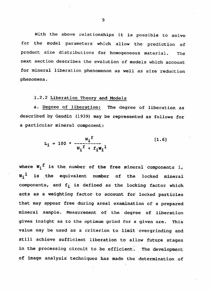
a. Degree of liberation: The degree of liberation as

described by Gaudin (1939) may be represented as follows for0

a particular mineral component:

*wif [1.6]Li = 100 ··v;;E—;·;;;:il -

where Wif is the_number of the free mineral components i,4 Wil is _the equivalent number of the locked mineral

components, and fi is defined as the locking factor which

acts as a weighting factor to account for locked particles

that may appear free during areal examination of a prepared

mineral sample. Measurement of the degree of liberation

gives insight as to the optimum grind for a given ore. This

value may be used as a criterion to limit overgrinding and

still achieve sufficient liberation to allow future stages

in the processing circuit to be efficient; The development

of image analysis techniques has made the determination of

10u

the degree of liberation of a mineral component a simpler

and less tedious task.

b. Liberation modeling: The first attempt aimed at

modeling liberation was that of Gaudin's (1939). He

proposed a model for the fracture of an_ideal binary system

composed of cubic components. From basic mathematical

relationships the percentage of liberated material that

could be expected was calculated. Furthermore, the concept

of a degree of liberation was introduced. In order to

quantify the degree of liberation, a. microscope counting

technique was described which allowed the estimation of a

particles composition. The model itself however, was

unrealistic since a cubic system was used along with cubical

fracture patterns which resulted in cubical particles.

It was not until 1967 that Wiegel and Li attempted to

modify Gaudin's model to allow a random orientation of

mineral grains rather than placing grains of least abundant

minerals as far apart as possible. A further modification

allowed this model to account for different mineral content

among composite materials. Though this model was indeed

improved from its previous version, it still was limited by

the cubic system assumption. -

With the advent of computerized image processing

systems in the late 1970's advances in the modeling of

liberation followed. King (1979) developed E1 model which(

11

was based on mineral grade distributions derived from lineargrade intercepts. It was assumed that the ore was .

isotropic, and had no tendency to fracture preferentially

along grain boundaries. Although this model was notably

better in predicting liberation values than previous models,

significant deviations from expected values were noted with

particles greater than 400 microns. This could have been due

to the assumptions that particles are isotropic and that

random breakage is the primary breakage mechanism. Contrary

evidence which indicates that preferential breakage is

present has been established (Choi 1982).

Following Wiegel's model, an attempt to model the

liberation of pyrite and ash from coal (Klimpel and Austin, ·

1983; Bagga and Luckie, 1983) utilized a Monte Carlo

Simulation technique to randomly create particles with

mineral grains. By making the computer generate specified

size distributions, the amount of liberation could be

· evaluated for different grinds. In general, this model was

developed for binary systems and was limited to random

fractures only. It also required that the amount of one of ·

the binary constituents be small in a composite particle (a‘

common occurrence in many mineral systems). The model

itself was validated with experimental data derived from·a

synthetic ore composed of polystyrene, pyrite, and quartz.

The excellent agreement between the model predictions and

12

experimental data gave credence to the assumption that

random fractures were dominant in this mineral system. _

Recently an index to describe the degree of liberation

was developed (Davy, 1984). The index varied from 0 to 1,

the value of which was found to be related to the shape and

size of the particles as well as to the interaction between

fracture surfaces and the structure of the mineral. Using

Davy's theory, a liberation model which utilized a random

Poisson Polyhedra for fracture and fragment distributions

from narrowly sized mono-sized particles was developed g

(Barbery,.1985).

Though much advancement in« liberation modeling has

occurred, the limiting factor of each model has been its

constraint to open circuit simulation. Each of the models

described assess the expected liberation that would occur,

but do not address the relative abundance of each type of

material composition. In the case of closed circuits, a

classification mechanism such as a hydrocyclone is affected

. not only by particle size but mineral composition as well.

For this reason, the introduction of varying amounts of

composite and liberated material back into the circuits

requires the knowledge of mass balances for each composition

of particles.

Initial attempts at the modeling of both size reduction

and liberation all encompassed limiting assumptions that

13

either made the model unrealistic with regard to physical

breakage phenomena, or did not provide accurate predictions ·

of liberation. Andrews and Mika (1975) modified the

population balance model for grinding to incorporate a

description of mineral particles in terms of size and

mineral content. The limitation with this approach has been

the estimation of the model's breakage and liberation

parameters. .

It was not until a variation on King's (1979) model,

which used linear grade measurements, that an- accurate

prediction of closed circuit behavior was observed. The

modification included the addition of a population balance

model to create a dynamic simulator which was validated with

pilot scale data (Finlayson and Hulbert, 1980).

Recent work at Virginia Tech has lead to the

development of a conceptually new modification “of the °

population- balance model for grinding. Along with the

breakage and distribution relations for all component

minerals, a liberation function has been introduced. Image

analysis data of areal grade measurements collected on batch

mill tests validated the model and the methodology behind

the solution of the model parameters (Choi, 1986).

Various methods have been developed for the analysis of

mineral liberation. The following section discusses the

14 _~

evolution in image analysis techniques developed by various

researchers.

1.2.3 Quantification of Mineral Liberation

a. Image analysis technigges: Along with the

development of models that have liberation terms included,

advances in image analysis have given researchers a

systematic tool to determine mineral liberation. Data that ,

is acquired for liberation studies is normally taken from

polished cross sections of mineral mounts. Prior to image

analysis, a variety of different methods existed to quantify

mineral liberation these included a linear intercept

technique (Rosiwol, 1898), an area tracing technique

(Delesse, 1848) and a point counting technique (Thompson,

1930).

An extension of the Rosiwol (1898) method of linear ·

intercepts was used by Barbery (1974) and King (1978) with

image analysis to_analyze grain sizes. The major limitation .

of the linear intercept technique is it's inherent

assumption that mineral species are isotropic.«

Two dimensional area measurements utilize the area of

mineral specimens to approximate mineral volumes. The

volume percentage of the mineralogical component is taken to

be the area of the mineral component divided by the total

area of the particle. A method known as "point counting"

evaluated the area of mineral components (Thompson 1930). ·

U15

V

It utilized a grid of dots which was superimposed over the

specimen surface to estimate mineral areas. The area was

assumed to be pmeportional to the number of dots on the

mineral surface. A modification of this approach was

described. by Guadin (1939). Gaudin's technique involved

placing a umno—sized mineral specimen 511 a briquette and

treating each particle as having the same size regardless of

its appearance. The mineral contents were then estimated as

a fraction of the particles total area, thereby eliminating °

errors associated with the briquette's orientation. Gaudin

. .also.„included. a "locking factor" to make the areal

measurement closer to that of actual volumetric values. The

"locking factor was used to reduce the overestimation of

liberation which arises from observing particles which may

only seem liberated. Image analysis equipment allows a more

exact estimation of mineral content by actually measuring

the relative areas of mineral components. Though image '

analysis has served to give more exact measurements, it is4

still limited to either the one or _two dimensional

approximations.

b. Volumetric Approximation Technigpes: In recent

years attempts have been made to approximate the volumetric‘

grades from both linear and areal measurements (King, 1982;

Bloise et al., 1984). The latest of such attempts has been

by the University of Utah. The method developed utilizes a

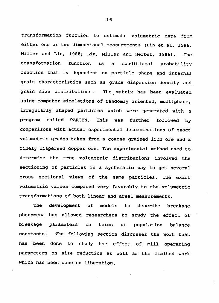
16

transformation function to estimate volumetric data from

either one or two dimensional measurements (Lin et al. 1986,

Miller and Lin, 1988; Lin, Miller and Herbst, 1986). The

transformation function is a conditional probability

function that is dependent on particle shape and internal

grain characteristics such as grade dispersion density and

grain size distributions. The matrix has been evaluated

using computer simulations of randomly oriented, multiphase,

irregularly shaped particles which were generated with a

program called PARGEN. This was further followed by

comparisons with actual experimental determinations of exact

volumetric grades taken from a coarse grained iron ore and a

finely dispersed copper ore. The experimental method used to-

determine the true volumetric distributions involved the

sectioning of particles in a systematic way to get several

cross sectional views of the same particles. The exact

volumetric values compared very favorably to the volumetric u

transformations of both linear and areal measurements.

The development of models to describe breakage

phenomena has allowed researchers to study the effect of

breakage parameters in terms of population balance

constants. The following section discusses the work that

has been done to study the effect of mill operating

parameters on size reduction as well as the limited work

which has been done on liberation.

17

1.2.4 Effect of Mill Parameter Changes on Homogeneous

Grinding

The major benefits that can be derived from being able

to quantify changes in mill parameters and their subsequent

effects on the basic grinding model are two fold. Assuming

that the population balance constants could be predicted for

different mill operating parameters, it would be possible to

allow studies on optimization of existing operations.

Moreover, the model could be more suited to scale up

applications and would replace the "Bond like" approaches

that have been used greatly in the past.

As discussed briefly in an earlier section, little work

has been done on the effect of mill parameters on liberation

and their subsequent role in modeling. In general,

themajorityof the studies related to mill parameter effects

have used homogeneous feeds. °

Results from various investigations have concluded that

breakage rates in dry batch ball mill experiments are highly

dependent on the mill environment and operating conditions.I

Breakage distribution functions seem to be a material

property and. are generally considered as being invarianti

(Herbst and Fuerstenau, 1972). With this in mind, an

analysis of breakage rates would yield great insight into

mill performance.

18

The basic grinding equation, though very useful, does

not allow for prediction of product size distributions under

different mill operating conditions. Experimentally

determined model parameters are valid for a constant set of

mill conditions.

In an investigation done by Herbst and Fuerstenau

(1973), it was concluded that mill speed and mill charge ‘

have a great influence on breakage rates; however the

resulting changes· in breakage rates were energy

normalizable. For a variety of different mill speed and

mill charge combinations, it was found that plotting the·

mass fraction of mono-sized feed remaining versus the

specific energy input yielded one line, the slope of which

was the specific breakage rate siE. A simple modification —

was then made to the general grinding equation providing the

following normalized relation:

SiEmi(E) + bij [1.7]u

where the energy specific breakage rates (SiE; i=1,n—l) and

the set of breakage distribution functions (bij; j=1,n;

i=j+1,n) are approximations of the model parameters which

are independent of mill speed, ball load and particle load '

within normal operating ranges.q

19

The resulting relation was then confirmed by predicting

product size distributions for different mill speed, ball

load, and particle load combinations. It was also found

that the ratio_of grinding times needed for the production

of the same product size under two different conditions (of

mill charge and speed) was equal to the inverse ratio of the

specific power inputs.

Other work that has been done in the area of' mill

filling has determined that increasing the interstitial

filling increases-the breakage rate up to an optimum, above‘

which a decrease in breakage rates is noted. (Houillier, ·

Neste, and Marchand, 1976) Similar findings have been found

with mill speed yielding maximum breakage rates at 70 to 85%

critical speed. ln order to determine the combined effectsof mill operating parameters Forssberg and Zhai (1987) used _

a factorial design approach to study ball charge, millV

speed, feed charge and pulp density on grinding fineness and ·

net energy consumption. Analyzing the derived response

surfaces, it was found that charge volume has a significant

effect on product fineness and net energy consumption. It

was also noted. that for· a given energy consumption, the

importance of operating variables in a decreasing order is

as follows: charge volume, feed charge, mill speed and pulp

density. Both grinding fineness and energy consumption were

found to be very sensitive to charge volume, yet relatively

20

insensitive to pulp density. Mill speed was found to have a

more pronounced effect on fineness than on net energy

consumption. Acceptable ranges for ball charge were found to

lie from values of 30 to 35% of the mill volume. Mill speed

ranges that provided acceptable results ranged from 70 to

85% of critical speed. Volume density ranges varied from 40

to 60%.

Other attempts at studying the effect of mill filling

include an investigation conducted by Austin, Smaila, Brame

and Luckie (1981). The general objective was to establish a U_ functional form for breakage rates using the fractional

filling of balls and the interstitial filling as variables.

From, batch tests a minimum specific grinding energy was

determined by using several combinations of both the

parameters studied. Further analysis of the data in terms of7

specific energy values demonstrated contrary evidence to

Herbst and Furstenau (1973). The results indicated that3

specific energy is not independent of ball load, and that an

increase in ball load from 25% to 40% of the mill filling .

would increase the specific grinding energy 8% while the

capacity increased by 16%. The discrepancy was concluded to

be possible experimental error on the part of Herbst and

Furstenau (1973).

A common finding by various investigators has been that

an inverse proportionality exists between a breakage rate

21U

and the corresponding particle loading. This was found

toholdtrue in the case of high mill loads for Gupta and Kapur

(1974).

Another operating· parameter which has been known to

cause significant changes in the breakage rates and overall

performance of a ball mill is that of ball size. It is an

accepted phenomenon that for every set group of mill

conditions there exists an optimum ball size that will yield

the greatest breakage rates. In addition, it is also

recognized that as particle size increases the optimum ball

size increases as does the breakage rate. (Kelsall, Reid, ‘

and Restarick, 1968; Kuwahara, 1971) An investigation by

Gupta and Kapur (1974) developed a functional relation·to

predict the effect of ball size on breakage rates. Upon .

inspection of other work that had been done in the area of '

ball size effects, the following relation was noted between

.the selection parameter Si(B) and the ball size B:

. $i(B)*

· w-——-—;——-—-= Q [(B-B°)/(Bi —B°)] [1.8]$1

where $1* is the maximum value of the selection function forthe ith size interval corresponding to the optimum ball size

Bi*, and B9 is a constant interpreted as the smallest ballu

size required to achieve meaningful grinding of the smallest

particle size of interest. <b is a unimodalz frequency

( 22

function which may be determined by plotting (B- BO)/(B*-B°)

versus S/S*. The resulting curve dictated the choice of a

Cauchy distribution and a simple mathematical relation was

then developed to predict breakage rates, based on the

derived functional relationship. The resulting expression

was quite consistent in reproducing breakage rate data that

was presented by Kelsall, Reid and Restarick (1968) for

quartz in a wet mill. (

A similar paper presented by Austin Shoji and Luckie

(1976) also provided a functional form to predict the

breakage rates attainable under different ball diameters.

The technique employed for fitting the data required the

introduction of various assumptions so that the estimation

method for fitting could be employed. Assuming that the

breakage rates attained by a mixture of balls approximates

the weighted mean breakage rates of the individual balls,I

some analysis was done in the predicting of a two

compartment cement mill with different ball sizes

ascomparedto a single ball size mill. Using the derived

relations, it was predicted that using a larger mix of balls

in the first compartment and a smaller mix in the second

compartment, would yield a 7% more efficient system than the

same amounts of balls in a single mill. It should be notedI

however, that the original derivations of the relations were

23

also based on data acquired by Kelsall, Reid and Restarick

(1968).

Since both of these papers were based on rather limited

experimental data, Gupta, Zouit, and Hodouin (1984) ‘

continued the study selecting a variety of different

materials including quartz, limestone, soft cement clinker

and a hard cement clinker. The first stage of the project

was to determine the error associated in mill scale up by

manipulating the mill diameter and the correspondingballsize.

Extensive errors were incurred when scaling up to a 3

meter mill from 10 and 15 inch mills. Error factors of as

large as 1.75 were obtained in the approximation of breakage

rates. This yielded ranges from 43% lower to 75% higher

values than the correct values. The large fluctuations were

due to the accuracy of the original breakage rate estimates

encompassing anywhere from 5 to 10% error. In eider to

minimize the errors the mineral was preground and more care

was taken to ensure a closer size range in the batch mill

feed. The functional. forms developed included. constants

that were material independent and predicted breakage rates

in 90% of the cases that were within 1% error of actual

experimental values. In all the cases studied, different

materials yielded radically different values for the

material constants. Therefore, it was concluded that a

~general equation proposed by other researchers is not

24

possible since different materials react differently to ballsize and mill size changes.

It should be noted that even though the majority of theball size experiments have been conducted on single ballsize loads, industrial operations involve a distribution of

ball sizes. This could, be responsible for some of the

significant errors associated with population balance scaleup values. With this in mind a recent study by Lo and ·

Herbst (1986) utilized a distribution of ball sizes in hopes

that it would improve the accuracy of scale up predictions.

Their experiments were conducted using choices of mill

speed, ball load, particle load, solid percentage, and ball lsize distributions that are typically used in industry. A

procedure was developed that allowed laboratory experiments

to be performed with the same ball size distribution as that

of a plant. The procedure involved plotting the' energy

specific breakage rate versus the particles size for each

ball size distribution. The resulting curves intersected at

one pivot point with each type of material. These values

were then utilized to develop functional relationships which

predict the energy specific breakage rates at various ball

sizes. Breakage distribution functions were observed to

change only slightly with ball size. This allowed initial

estimates of distribution functions to be used regardless of

25;

a change in ball size. The resulting predictions for the V

variety of minerals tested provided excellent results.

Most of the grinding experiments that have been

conducted have been dry batch tests. In the case of wet

grinding, it has been noted by several researchers that

breakage rates significantly increase for the larger size

classes. This general trend is not as prominent for smaller

size classes (Fuerstenau and Sullivan, 1962; Berube, Berube,

and Houillier, 1979). Another well know phenomenon is the

inherent increase in the breakage rates with time for wetV grinding. Though these breakage rates could be fitted with

empirical relationships, the resulting values would have no

true physical significance in as far as the classic grinding

model is concerned. In order to analyze breakage rates the

initial slopes of the disappearance plots have been taken to

be the representative values. (Tangsathitkulchai and Austin,

1984) _

26

1.3 RESEARCH OBJECTIVES

The objective of the present investigation is to

develop a general understanding of how changes in ball mill

parameters affect breakage rates of liberated and composite

particles. The eventual goal of this study is to see if

liberation can be affected independently of size reduction.

If this were in fact the case, then mill design could be

improved on the basis of liberation. Though this study is

fundamental, it is hoped that it will yield a valuable

insight into the breakage characteristics of composite

minerals and a conceptual grasp of how mill parameters may

affect liberation.

All breakage rates are analyzed in terms of energy

Inormalized values (Ton/kw hr). The normalization or non-

normalization of breakage rates will yield clues as to which

breakage rates will require functional forms in terms of a4

liberation model. As noted in the iliterature review,previous work has been limited to studies on homogeneous

material. Though the past information gathered is helpful,

it does not address the key role of grinding which is

liberation. It is for this reason that this project has

been designed to study the effect of mill speed, ball size,

mill charge and wet vs dry grinding with particular emphasis

on the breakage of composite particles. It is hoped that

the information gathered can act as a precursor in the

27

development of a liberation model that predicts both mineral

product size and the degree of liberation attainable under

varying mill operating conditions.

CHAPTER II.

EXPERIMENTAL PROCEDURES

2.1 Ore Sample ~

The -ore sample used for this investigation was

basically a binary ore composed of coarse grained sphalerite

and dolomite. Its coarse liberation size simplified the

analysis of the mineral system by image analysis.

Furthermore, the relatively large contact zone between both

mineral species, was desirable in studying liberation. It

was acquired from ASARCO’s Young Mine which is located in

Jefferson City Tennessee. The processing plant treats

approximately 7,700 tons/day of ore. The ore itself has a

grade of approximately 3% zinc. The preparation stages ·

involved, at the sight include two stage crushing, heavy

media separation, followed by ball milling and finally a ·

flotation circuit.

The heavy media separation device, which uses

ferrosilicon, processes 250 tons/hr of ore. The basis for

this technique utilizes differences· in the specific

gravities of sphalerite (4.0 SG) and dolomite (2.8 SG). The

heavier ore particles containing sphalerite sink while the elighter particles float yielding nearly 77% of the dolomite

dominant particles as tailings.

° 28A

29

The total sample weight which was acquired was 1500 lbs

of concentrated ore from the heavy media circuit containing

nearly 14% zinc. The sample consisted of particles that

were 2 to 3 inches in size.

2.2 Grinding Equiment and Torque Measurement

The batch grinding experiments were conducted in a

stainless steel mill measuring 25.4 cm in diameter and 29.2

cm in length, with lifters spanning its length. The mill

rested on roller bearings and was connected to a .5 horse

- - power electric motor. The shaft which linked the two had a

Brewer Engineering Laboratories model A-055 torque

transducer. The output from the torque transducer was

displayed. on. a Brewer Engineering Laboratories model DJ-

335A/2 digital readout sensor.

The mill's operating characteristics are described by · .

Yang et al. (1968). The balls used in the mill varied from

3/4-inch, 1-inch and 1- 1/4-inch balls, the weight of which

in all cases was approximately 30 Kg. The volume filling of

the balls occupied approximately 50% of the mill.

2.3 Sizing Equipment 4Standard eight inch diameter Tyler series sieves

ranging from 10 to 400 mesh were used in combination with a

model B Ro-Tap machine. A Mettler AC 100 balance was

30

employed to measure weights providing an accuracy of i .01

grams. It should also be noted that a standard wet screen

shaker was used to perform a more efficient wet screening.

2.4 SEM¤IPS Image Analyzer

A Kontron Scanning Electron Microscope—Image Processing

System (SEM-IPS) was used. to collect image analysis data

(see Fig. 2.1). .This system was designed to either acquire

images from an energy dispersive SEM or from a video input t

which monitors a mineralogical microscope.

The following is a list of the actual hardware which

made up the system: Zilog Z80A (4MHz) processor with 64

KByte dynamic system RAM, 8 Bit data bus, 16 Bit addressn

bus, 20 MByte Winchester hard disk, 600 KByte Floppy disk,

CRT controller for alpha and graphic monitors, 2 serial

ports RS—232—C, slow scan interface, scanning” stage

interface and an autofocus interface.

The actual image processor unit had the following

specifications: array processor with pipeline structure,

hardware multiplier, 16 Bit ALU and 6 KByte microprogram

memory, 8x256 KByte image memory, additional 2 MBit for

overly or parity, variable format image storage, standard

512*512 pixels at 256 grey level values plus 1 bit parity,

and a A/D converter for the TV—signals. The high resolution

32

color monitor had a band width of 20 MHz (+/-3db), 800 lines

/ 50Hz or 640 lines / 60Hz.

cemmänds, program listings, and graphics were displayed

on a black and white monitor. Access to program commands

was achieved by an ASCII keyboard and a cügitizer tablet

with a crosshair cursor. Hard copies of data, graphics or

program listings could be made with a OKIDATA, Microline 82A

printer.

The actual image source for the experiments conducted

came from a Zeiss Inverted Camera Microscope, type 405. The

link between the microscope and the SEM—IPS system was a

Dage MTI 86 Series mounted television camera. 4The IPS software available for this system allowed

enhancement of images and processing of data. It also

allowed. the distinctionof’

objects on the basis of' grey

levels as well as geometrical shapes. Whichever the method

of distinction used, the final objective of the system wash

to separate the objects to be studied from the background.

This process, which is termed discrimination or

segmentation, is normally done by grey level threshold

values which the operator has designated. Pixels that fell

into the selected grey level ranges were converted to a

binary 1. All other pixels, which were not in the specified

range, were converted to binary 0. This binary image

assumed a black and white color with the objects of

33

interest. This image was then used to provide either field

or object—specific measurements.

Discrimination was facilitated by a variety of image

processing procedures such as spatial filtering, contour

enhancement, shading corrections, etc,. After the image had

been discriminated, further processing of the image

eliminated errors due to noise. A criteria was then used to

selectively choose particles on the basis of size or shape.

It was also possible to interactively edit grey levels on

the created binary images.

~ All changes that were affected by the processing

commands were evident on the high resolution screen. The

actual commands were depicted on the host processor monitor

which had a menu that allowed access to all the processing

routines. To select an image processing routine a mouse was

utilized which moved a cursor throughout the screen. Input .

variable numbers were entered with the keyboard.

The variety of functions chosen were all storable as a

program. once established. a program was executable with a

single command.A

2,5 Experimental Procedure .A ‘

2.5.1 Sample Preparation

The ore which. was acquired from the mine measuring

approximately one to three inches in size was passed through

34

a 5x6 inch laboratory jaw crusher. This material was then

passed through a 8x6.5 inch hammer mill so that the final

product size was -10 mesh. Narrow size fractions were then

prepared by sizing the hammer mill product.

2.5.2 Grinding Experiments

The ball mill used to do all the batch grinding

experiments for this study is described in section (2.2).

In order to study the effect of mill speed, tests were

conducted at 40 and 85% of critical speed. In each of these

cases, a 1 inch ball size diameter and a feed of 3000 grams

was used. The closely sized feeds were ground dry for 1, 2

and 4 minute intervals. In studying ball size, a 75%

critical speed was used for all the tests with a charge of .

3000 grams per test. Ball size tests of 1, 2, and 4 minutes

were conducted for each of the ball sizes of 3/4, 1, and 1-

1/4—inch diameter. Mill charge tests were conducted at 75% -

critical speed. with a. 1-inch. ball size for each of' the

charges of 3000, 4500, and 7100 grams. With the exception

of the 3000 gram charge which was conducted for 1, 2, and 4

minute intervals, the remainder of the experiments were

conducted only at 4 minutes to conserve material.

At the end of each grinding time, the mill was kept

stationary to avoid the loss of fines when opened. The mill

was then emptied and special care was taken to collect all'

fines adhering to the mill. All samples weighing 4500 grams

35

or less were then split into eight portions. The 7100 gram

run was split into sixteenths due to the large amounts of

material present in each size class. These splits were then

weighed and later dry screened c¤1 a Ro-Tap sifter for a

duration of 15 minutes, to produce size fractions ranging

from the top size class down to -400 mesh material. Dry

screening was then followed by wet-screening to remove fines

from each of the classes. The material which passed during

the wet screening was then added to the next size class down

to avoid loss of material. The loss of material never

amounted to more than .1% of the total charge. The samples

were then dried, weighed and bagged for later use in the

preparation of briquettes.

2.5.3 Briggetting and Polishing

Material from each size fraction of interest was

representatively split into approximately 10 gram samples _

and added to 1 inch diameter molds. Cold setting EPOFIX

Epoxy was then added. to the mold and. the briquette was

placed under a vacuum in order to remove excess air bubbles.

The mold was then allowed to sit overnight. Once the epoxy

had hardened, the briquettes were then cut into 5 vertical

cross sections using a Buehler Isomet Low Speed Saw. These

slices were then remounted in epoxy resin and allowed to

harden. This procedure was implemented to avoid orientation

36

effects which have been found to cause error in previous

studies.(Choi, 1986).V

The particle mounts were then polished by using a 600-

grit metal- bonded diamond lap followed by polishing on a

canvas using 600-mesh silicon carbide as an abrasive. The

final stages of polishing included the use of 6-micron

diamond paste on a TEXMET pad, followed by the use of a

Syntron Auto Polishing machine with .05 micron alumina

powder for a period of 10 hours.

2.5.4 Liberation AnalysisL

In general the image processing procedure can be

illustrated by Figure 2.2. An analog image from the

microscope was digitized on the high resolution monitor. The

image was then enhanced and processed in order to facilitate

the accurate extraction of the objects of interest. Once

extracted the defined objects were then converted to binary

images of white on a black background. At this stage the

area measurements could be made on the selected objects in

either an object or field—specific manner. ·

In order to obtain liberation data, the polishedI

briquettes were analyzed using the SEM—IPS image analysis

system. The system was used to provide areal grades of each

particle. Areal assay data from each particle was printed

out and stored on a floppy disk.

37

eps MEAsum~6 pnoamum

¤MA6E IMAGE mpursouncs ll

svsrsm ssrup

llGRAY IMAGE pnocsssmell

nmsmcnva EommJ!ssemenmnowll

BINARY uvmas Pnocassme

PARAMETER seuzcnonJ!

MEASUREMENTl.

J!mm ourpur

sromxcauz om onsx

¤«s¤>LAv PRINTER

Figure 2.2 Image Processing Procedure

38

An attempt was made to implement the transformation

program developed by Lin (1985) to convert the areal data to

volumetric approximations. The output from the program

provided results that were not credible or physically

possible. In addition to providing negative values for

masses in certain grade classes, some grade classes were

reported to have more mass after a 2 minute grind than a 4

minute grind. These discrepancies could be attributed to the

small amount of material that was associated with the

problematic grade classes. In general, the program seems to

be limited to mineral systems that have an even distribution

of grade classes.

With the absence of an adequate volumetric -

approximation technique, the areal values were taken to be

equivalent to volume. All the particles were presumed to be

the same size in the measurement of areal upercents

regardless of the apparent size under the microscope. This

assumption was taken since each briquette was composed of

closely sized material. The free particles observed were

taken to be liberated material and were not corrected by the

use of locking factors. The weight fractions of each

particle class were then obtained by multiplying' by the

specific gravity of each component. The mass ratios of each

class could then be obtained by using a simple program to

selectively keep track of masses in terms of predesignated

39

grade classes. In order to have a larger number of

observations per class, the ranges of 0-5%, 5-50%, 50-95%,

95-100% sphalerite were used to quantify the distribution.

The two extreme cases of 0-5% sphalerite and 95-100%

sphalerite, were assumed to act as liberated material for

the purpose of data analysis.

2.5.5 Statistical AnalysisThe two types of error associated with image analysis

measurements are that of operator error and statistical

error incurred if too few particles are counted. The error

which is due to the operator is significantly reduced with

experience. Statistical error can be evaluated with a °

statistical analysis described by Jones (1982) and Lin etal. (1985). This same method may be employed to determine

the amount of _particles required to acquire an unbiased

representative sample of a real or linear gradedistribution. ·Since particles are randomly distributed in the epoxy

matrix, the best estimate of the density in the i-th grade

interval (fi), and the relative error (Si) may be describedby the following relation:

V

j=1fi = --—-—- x 100 [2.1]

EnW-~ j=1 J — .

40

and

fi‘ Sfi = -;/1;———·— [2.2]

where

n = total number of observationsI

ni = number of observations in the i—th grade interval

Wj = weighting factor for a given observation: Wj = l

for the measurement based on number, Wj = lj forthe measurement based on length where lj is the

intercepted length of particle j.

fi = percentage in the i—th grade interval

Sfi= standard deviation which is the expected accuracy

of the analysis of the percentage in the i-th

grade interval »

Equation [2.2] may be used to establish the smallest

number of observations required to produce iaccurate

estimates of volume fractions of the components. If the

number of composite particles amount to 10% of the total

volume and are randomly distributed within four grade

intervals, then fi = 2.50. For an expected accuracy of 5%

(Sfi=.05), the minimum number of observed particles would

be:

¤= ( ——fi——)2 = 2500

41

With this calculation in mind, particle counts were

maintained at 2500 and above to ensure precise measurements

for all the experiments conducted.

CHAPTER III .

EXPERIMNTAL RESULTS

In order to establish breakage rates a sequence of

batch grinding experiments were conducted on a coarse

grained sphalerite ore. The breakage rates for particles

with different sphalerite content were evaluated. with an ‘SEM-IPS image analyzer.

‘ 3.1 Comparison of Image Analysis Results Against CheicalI

Assays _

Table 3.1 illustrates the assay results from image

analysis and chemical assays and the relative error between

both for two sample specimens. The procedure used for

chemical analysis is located in Appendix V. It should be

noted that quite accurate results can be obtained with image

analysis techniques.“

TABLE 3.1 ·Comparison of the zinc content determined with _· image analysis and chemical assays.

Size Image Chemical(mesh) Analysis (X1) Assay (X2) Error*

10x14 8.85 8.54 3.63I

14x20 14.43 13.44 7.37

”42

43

X1-X2*Error = -——-———— x 100

X2

The slight overestimations of grades with image

analysis can be attributed to the lack of locking factors.

Some of the particles observed may have seemed liberated due

to their orientation, when in actuality they were locked.

Nevertheless, the close approximations of areal grades to

chemical grades verifies the accuracy of the sample

preparation and the experimental procedure involved in this

study.

3.2 Feed Characterization

An example of a feed characterization for one of the

narrowly—sized feeds used is illustrated graphically in

Figure 3.1. The characterization data for all the feed·

samples are located in Appendix I under Tables I—1 through I

I-10. For the purpose of analysis, material that contained

less than 5% or greater than 95% sphalerite was assumed to

act as free material. It should be noted that the majority Iof the feed material was already free leaving only

approximately 10% of the material as composite particles.

This liberation phenomenon can be explained by the large

grain size which is inherent in this mineral system.

4 4

,SphaleriteQ40% Critical Speed

Percent ol Feed Mass

80

00

.Q...................................................•.....•..... 3

Q20 1 2.61

6.360-5 5-50 50-95 95-100 ·

5 ‘Sphalerite Content (VVt %)

145:20 mesh QFigure 3.1 Example of a 14x20 mesh feed distribution for

a 40% critical speed test.

‘45

3.3 Determination of Breakage Rates

The top feed size breakage rates (selection functions)

for liberated and composite classes may be determined by the

disappearance of this material from the original narrowly-

sized feed. Since material can only break into smaller

sizes, it is possible to plot the fraction remaining verses

time for a given feed composition. Since the amount of

material which is liberated and composite can be quantified

by image analysis, a single series of grinding tests can

provide breakage rates for all classes of particles. X

The determination of the top size breakage rate for a °

particle class of composition x is carried out by grinding

the total ore in a batch mill. In this example, mxl(0)=1

and mxi = 0 for i=2,....N. Equation 1.2 then becomes:

‘*“‘1" X X X X**'' = S 1 °!l1 1(t) [3.1] .dt ·

where mxl is the mass of material that is of size class 1 ’

and a composition of x.

Solving for the breakage rate of size 1 and composition x:

m"1(t>—SXl(t) = ln —————— [3.2]

. IIlxl(O) 4

46 ‘

Thus the slope of a plot of ln[mXl(t)]/mx1(o) versus time

which by convention is know as a disappearance plot, is

equal to -Sxl. ·

Figure 3.2 is an example of a typical disappearance

plot. The disappearance plots for the various experiments

conducted under different operating conditions are located

in Appendix III. Included in these illustrations are plots

for material that ranges from 0-5%, 5-50%, 50-95%, and 95-

100% sphalerite. 'In general, the disappearance plots were _

either first order with some data scatter, or concave

(indicating a decreasing breakage rate with time).

Therefore, initial breakage rates were used whenever

possible to compare the various conditions studied. The

distributions acquired for all the experiments are located

in Appendix I under tables I-1 through I-10. The actual

calculated percent remaining values that were plotted are

located in Appendix II under tables II-1 through II—l0.

47

10 X’„$_DO\ä

Q ,Ol

E 1E

1O

g 10OC

+-·E 1Q)O 0 0-5s SPHAL

0. ¤ 6-606; SPHAL_A 50-95s SPHAL

>< 95-10066 SPHAL1

*0 1 2 :6 4 *16Time (mm)

Figure 3.2 Example of a disappearance plot for 14x201

mesh feed at 40% critical speed.

48

3.4 Determination of Energy Specific Breakage Rates

In order to determine Energy Specific Breakage Rate

values, the following relationship was employed:

SE = S H/P (60min/lhr)

where

SE = Energy Specific Breakage Rate (Tons/kwhr)S = Breakage Rate (1/min)H = Hold Up in Mill (Tons)P = Power (kw)

The displayed torque values in inch—pounds and the

corresponding revolutions per minute were used to calculate

the power applied to the shaft via the following

relationship: .· P = (2un) T

where ·‘

P = Shaft Power Input (in—1b/min)T = Torque (in-lb)n = Revolutions Per Minute

Converting to Kilowatts, the equation becomesI

P = 1.182 x 10-5Tnwhere .

P = Shaft Power Input (kw)

The conversion of the mill hold up from grams to tons

is as follows:

H = (feed in grams) x 1.10229 x 10"6 Tons/gram

The values obtained for the calculated. breakage and

energy specific breakage rates are located in tables IV-1

through IV—4 in Appendix IV. The following section attempts

49

to quantify the effect of experimental error on these

calculated values.

3.5 Effect of Image Analysis Error on Breakage Rate

Calculations

In order to quantify the effect of image analysis error

on Breakage rate calculations, particle counts for a 10x14

mesh sample were varied in increasing order of abundance up

to 3000 particles. The resulting weight percent fractions

for each class were compared for 2000 and 3000 counts.

Table 3.2 illustrates the results obtained and the relative

error between both initial breakage rate estimations.

TABLE 3.2 Effect of Image Analysis Error on Areal Grades.

_ %BY WEIGHT OF TOTAL MASS .Particle 2000 Particle 3000 Particle Deviation Relative*

Class Counts (X1) Counts (X2) From Mean Error

0-5% ‘81.34 81.11 .115 .14%

5-50% 6.97 7.68 .355 4.85%50-95% 3.09 2.60 .245 8.61%95-100% 8.59 8.60 .005 .06%

*Deviation From Mean = ABS(X1—X2)/2

ABS(X1—X2)/2*Relative Error = —-—--—--—-—— x 100

(X1+X2) /2

The 3000 particle count sample was taken to be the most

accurate approximation, thereby allowing an evaluation of

”50

S

the error taking a conservatively lower number of particle

counts (ie. 2000). It should be noted that the liberated

mineral components have negligible error and therefore

require much fewer particle counts to get accurate weight

percent approximations. Table 3.3 illustrates the error

associated with calculating breakage rates for an experiment

conducted at one, two and four minutes at 40% critical speed

with a 1" ball size and 65% interstitial filling. The

values of "deviation froua mean" in table 3.2 are either

added to, or subtracted from, the weight percent values to

give positive or negative error values, respectively.

TABLE 3.3 Analysis of Error Associated With Image Analysisin the Calculation of Breakage Rates.

BQZBZBZB'°°'''''''SBZSSZZZ;B'BZ.ZZZZB,B°Z.ZZB'BZBS'“''''''“''''Class Negative Error No Error Positive Error'''“'BIBB''''°°''ESBZ'''°'°°“''ESZB°'''°’“°“'ESZB''“'°'''

5-50% .3583 .3546 .351050-95% .2670 .2652 .263495-100% .2495 .2595 .2494

Even though. image analysis was expected to be the Vprimary source of error, it can be seen by table 3.3, that

very little error was introduced even if a conservatively

small number of observations are taken. It should be noted

that the rest of the experiments conducted in this

investigation were also expected to behave in a similar

manner.

51

The calculation of energy normalized breakage rates .

involves the measurement of both the revolutions per minute

as well as the torque. From the standard deviations that

were incurred, it is estimated that the error associated

with these measurements did not exceed 1.3%. This small

amount of error would have very little effect on the

calculated energy specific breakage rates.

CHAPTER IV.

DISCUSSION OF RESULTS

4.1 Analysis of Braakage Rates

To simplify the analysis of the breakage rates in terms

of composition and operating parameters, plots have been

generated °in which the breakage rates have been plotted

versus the percent sphalerite class for each parameter. The

mill speed parameter for 40 and 85% critical speed is

illustrated in Figure 4.1. These values were chosen since

75% critical speed represents a normal operating condition

of a ball mill and the other two values would be considered

extreme operating conditions of cascading and cataracting

environments. From this plot it can be noted that the 85%

critical speed provides the greatest breakage rate for all

the particle classes. In going from 40 to 85% critical

speed there is a shift in the optimum breakage rate for

composite classes from 5-50% sphalerite to 50-95%

sphalerite. This shift could be attributed to the actual

kinetics within the mill changing from a predominantly

cascading environment to one which has·a cataracting zone.

This would tend to indicate that the material which consists

of 5-50% sphalerite is more apt to break preferentially

faster under attrition conditions than the 50-95% sphaleriteI

material which is more apt to break faster under impact

lu52

u

53

1.00

0 40% CRITICAL SPEED

A 85% CRITICAL SPEED

/80.75 A\1—\./ -

A*:3% 0.60 6 1A

q) 0

O0

OL.

CD

°·°°0 20 40 60 80 100Volume % Spholente

Figure 4.1 Breakage rate versus perCeI1C sphalerite plotsfor different mill rotational speeds withl4x20 mesh feed.

54

conditions. This phenomenon could be explained by the fact

that sphalerite is more brittle and therefore is more apt to

break under cataracting conditions. It follows that

particles which have a higher sphalerite content would tend

to break preferentially in a cataracting environment. This

is also supported by the fact that the increase in breakage

rates, associated with an increase in mill speed from 40 to

85% critical speed, is more prominent for sphalerite rich

material.

In analyzing the effect of ball size, Figure 4.2 shows

that a 1- inch ball size is the most effective in reducing

10x14 mesh feed for all composition classes. It is also

apparent that the breakage of classes consisting of greater‘

than 50% sphalerite are significantly enhanced with the

usage of the 1 or 1 1/4 inch ball sizes. This increase in

breakage rates is much less apparent for material consisting

of less than 50% sphalerite, indicating that the degradation

of dolomite is less susceptible to a change in ball size. A

possible reason for this phenomenon is that the ball—ball

interaction or energy input due to friction remains

relatively similar, while the impact energy of cataracting

balls changes greatly with different ball masses. This once

again supports the contention that sphalerite rich material

_ seems to exhibit improved breakage under impact conditions.

66

1.50

6 3/4 in BALL sezs

1-25 ¤ 1 in BALL SIZE,.„ A 1 1/4 in BALL snzsc:\1.00 /^i"\./

4*3 0.75 ÜO A

IG) 1

o '

0:U

¤ .E 0.25

G)

°·°°0 „ 20 ~'• 60 80 10Volume x Spholente

Figure 4.2 Breakage rate versus percent sphalerite forvarious ball size diameters with 10x14 meshfeed.

56

It is also interesting to note that an increase of ball

size to 1 1/4" provides similar values of breakage rates as

the l" ball size. This would tend to indicate that the true

optimum ball size could be between l" and 1 l/4" diameter.

Impact energy seems to be a function of both momentum and

contact area. Increasing or decreasing the ball size from

the optimum value, has a detrimental effect on impact energy

by influencing momentum and contact area accordingly.

The effect of mill charge yielded similar results to

the other parameters in that an optimum value of

interstitial filling ·was found that resulted in enhanced

breakage rates for all compositions of particles (see Figure

4.3). An interstitial filling of 65% was found to be the

most efficient in breaking 10x14 mesh material with a 1"

ball size. Increasing the amount of charge to 150%i

interstitial filling decreased all the breakage rates and -

had an even more significant effect on the composite

classes. At 150% interstitial filling the composite classes

had lower values of breakage rates than either the dolomite

or sphalerite.u

This would tend to imply that an

overcharging of the mill impedes the breakage of composite

materials as well as sphalerite. The possible cause for the

lessening of the breakage rates is the cushioning effect of

the excess mineral and its associated reduction of impact

energy to particles. _It is of great interest that this

57

1.25 I .

o 65x FILLING

¤ 100% 1=1u.n~16 °/-\1°OO A 150z FILUNG

E

uunw. BREAKAGE RATE1* 0.75x./ OG)-•—»

Q? 0.50 Q0 0/ 4·—M|N BREAKAGE RATE

O ___ __ ..-¤-·* "' " "'..¥ ¤ —- " "°Oq) 0.25L AQ 4-um BREAKAGEmm;°·°°

• 20 0 40 60 80 100Volume $8 Spholerute

Figure 4.3 Breakage rate versus percent sphalerite forvarious interstitial filling with 10x14 meshfeed.

58 .

cushioning effect seems to be more effective with particles

containing sphalerite since this would indicate that these

materials are more susceptible to impact than liberated

dolomite.

Comparing 4.udnute grind data, wet grinding provided

enhanced .breakage of the 14x20 mesh feed in all the

composition classes, as can be seen in Figure 4.4. A

possible reason for the enhancement of breakage rates is the

inherent suspension of fines within the wet environment at

70% solids. It should be noted that the general increase in

breakage rates was more prominent for the classes containing

sphalerite, once again indicating that this material may be

more susceptible to impact conditions.

The lack of curvature on the dry grind can be

attributed to the fact that only 4 minute grind data was

available due to a shortage of 14 x 20 mesh material. With

this in mind, only the 4 minute grind data was used for the »

70 percent solids plot.

4.2 Analysis of Energy Specific Breakage Rates:

Since all of the parameter changes involved a change in

the energy draw from the mill, the breakage rate values were

normalized with respect to energy to see if the actual

breakage kinetics were changed as opposed to the changes

being simply a function of energy input. Plotting the

59

1.00

0 70% SOLIDS _

¤ DRY

/é;\0.75y°§ 4—·MlN BRBRKAGE RATE O

‘-—-xx

0

4-MIN BREAKAGE RATE_,‘B0.50 · ·/________________„——--——-¤

Ö(D

l.07

50.2VOQ)L

CD

°·°°0 ‘ 20 40 60 80 100Volume % Spholente

Figure 4.4 Breakage rate versus percent sphalerite fordry and 70 percent solids grindingenvironments with 14x20 mesh feed.

' 60

specific breakage rate versus the percent sphalerite, allows

the analysis of parameter changes in terms of energy

normalized breakage rates for each composition class.

Figure 4.5 illustrates the effect of a change in mill

speed on the energy specific breakage rates of 14 x 20 mesh

material. Once normalized with respect to energy, the free

sphalerite and dolomite components move much closer

together, however the composite classes still exhibit their

differing peaks. This indicates that changes in the mill

rotational speed could be considered energy normalizable for

the free components. If this were in fact the case, a

general liberation model could use a simple energy relation

to describe free particle breakage and a functional relation

to describe composite particle breakage. °

A change in ball size yields values for specific

breakage rates that vary greatly when an optimum b511 size

is used. The effect of ball size on energy specific

breakage rates can be seen on Figure 4.6. The l" and l l/4"‘

ball sizes seem to normalize with respect to energy, while

the 1/4" ball size diverges from the larger ball sizes. A

possible reason for the apparent normalization of the two

larger ball sizes could be that the optimum ball size range lis sufficiently large to provide similar breakage rates for

both sizes. Since the power draw for both of the larger

ball sizes were similar, it follows that the energy specific

61

2.000 4OS CRITICAL SPEED1.75

X A 85% CRITICAL SPEED

1.50':„

A

Q) 1.25-6-*O OCK 1.00 ^äÖ A

O--o

- AQ) 0$6 0.500EE3 0.25Q.U)

°·°°0 20 40 60 80 100Volume S Spholente

Figure 4.5 Energy normalized breakage rates versuspercent sphalerite for different millrotational speeds with 14x20 mesh feed.

62 ~

2.50

o' Z5/4 in BALL SIZE

eg ¤ 1 in BALL SIZEA 1 1/4 in BALL SIZE

OI-x./

2OIZ 6G)8’_ä 1.00 OL

U/Z

.9 0.60E'.:O(DQ.U) I L

°·°°0 20 40 60 80 100Volume $8 Spholente .

Figure 4.6 Energy normalized breakage rates versuspercent sphalerite for different ball sizeswith 10x14 mesh feed.

63

breakage rates would be comparable in magnitude.

Nevertheless, the divergence of the 1/4" ball size indicates

that ball size is not normalizable with respect to energy Ioutside the optimum ball size range. A liberation model

which accounts for ball size changes would require some type

of functional form to predict particle breakage.

The changes in energy specific breakage rates related

to changes in ball size are much more prominent for material

that is rich in sphalerite. In fact, as the amount of

sphalerite content increases the spread in the energy

- specific breakage rates also increases.

The effect of interstitial filling on the specific

breakage rates of various particle classes is shown on

Figure 4.7. From ·this figure it can be seen that free

dolomite tends to normalize well with respect to energy. As

the amount of sphalerite content increases, the Abreakage

rates become non-normalizable. Once again, it seems that

the differences in breakage kinetics within the mill for

particles containing sphalerite are more prominant. The

hindering of breakage rates for composite materials and

sphalerite is not a function of the increased power draw due

to more material, but a change in the breakage mechanisms.

It should also be noted that overcharging the mill to 150%

interstitial filling caused a significant hindrance of

composite particle breakage, more so than with liberated

64

2.50z·xJI

0 65% FILLING

{ ¤ 100;; F1Lu~cC zoo A 150ss FILLING 0C)I-~./ -Q) - ‘*6 1.50

INITIAL BRüKAGE RATE0

q) ____,.-¤CD__,O1.00

..--·—°‘“”'“"”_X U- -···’ OO A 4-MIN BREAKAGE RATE A

L.@ A

:4;- 4-MIN BREAKAGE RATEC)0)

1%°·°°

• 2 40 60 80 100Volume $8 Spholente

Figure 4.7 Energy normalized breakage rates versuspercent sphalerite for different interstitialfillings with 10x14 mesh feed.

65

material. This would tend to confirm that composite

particles are more susceptible to overcharging and the

associated cushioning effect. The introduction of mill

filling as a variable in a general liberation model would

require a functional form for material containing

sphalerite. On the other hand, dolomite would require a

simple energy relationship in the prediction of its breakage

characteristics. ·

Figure 4.8 illustrates the energy specific breakage

rates for a dry and 70% solids grinding environment on 14 x

_ _ 20 mesh feed. From the data collected it is apparent that A

the changes in breakage rates are non normalizable with

respect to energy. The inclusion of this parameter into a

generic liberation model would certainly require a

functional relationship to describe particle breakage.

4.3 Coparison of Experimental Results to Previous Werk:

It should be noted that direct comparisons to previous

work are not possible since these studies have been based on -

homogeneous material. It is possible however, to compare

trends that have been observed with changes in mill

operating parameters and there effect on breakage rates. For 4

the convenience of comparison, the collected data has been

plotted with the independent variable being the mill

parameter, and ‘thedependent variable being the breakage

66

2.00zw

§ 1.75\ 0 70% s0u0sC0 1.60 D DRYI-\/

(D 1 25 4-MuN BREAKAGE RATE46 l

°o——·—··"Z7O

1-ÜO O 4-14111 6REA1<AcE RME0* _„__.-.....——-——-——¤-—····""‘“"“"°O ¤—·—*""""°

.66 0.75OQ)L.

(D 0.50

.9•~•—

0 0.25q) .O- · . —

°·°°0 20 40 60 80 Y 100Volume % Spholerute

Figure 4.8 Energy normalized breakage rates versuspercent sphalerite for dry and 70 percentsolids grinding environments with l4x20 meshfeed-

67

rate achieved. This has been done for the ball size and

mill filling experiments with each of the compositions of

particles as can be seen on Figures 4.9 and 4.10.

In the case of mill speed, Herbst and Fuerstenau (1972)

found a mill speed of 75% critical speed provided the

optimum breakage rate of 7 2< 9 mesh dolomite. This was

accomplished by varying the mill speed from 30 to 90%

critical speed. From the two mill speeds tested in this

investigation, 85% critical speed was found to provide

substantially better breakage rates than that of 40%

critical speed for all the particle classes. However, the

enhancement of breakage rates due to and increase in mill ·

speed was much more pronounced for particles rich in

sphalerite.

Analyzing the energy specific breakage rates obtainedI

for the mill speed parameter, it was found that breakage

rates of the liberated components were generally

normalizable with respect to energy. Similar results were

presented by Herbst and Fuerstenau (1973) for the grinding ‘

of pure dolomite.

Figure 4.9 illustrates breakage rates as a function of

ball size. In general it can be seen that an optimum ball

size significantly increases the breakage rates for all the

particle classes. Similar responses to ball size changes

were observed by Gupta and Kapur (1974) and Gupta, Zouit and

l 68

1.50

0 0-5% SPHAL

¤ 5-50% SPHAL1-25 A 50*95% SPHA1.

X 95-1ÜÜS SPHAL°Eä1.00 x\

€—

\/

Q)46 0.75 A___0: °\go 50 ° "O

•

Ä.S

/CD 0.25

°·°8.60 0.75 1.00 1.25 1.50Boll Suze (nn)

Figure 4.9 Breakage rate versus ball size for different· sphalerite content material with 10x14 meshmaterial.

69

Hodouin (1984). Both investigations as well as others have

shown that the use of a ball size other than the optimum

results in significant drops in_breakage rate values. It

should be noted that the effect of ball size on breakage

rates increases with the amount of sphalerite present. In

the case of the 0 to 5% sphalerite class, little change was

noted as a result of ball size. Dolomite's low sensitivity

to ball size changes would tend to explain the lack of a

clear maximum value for this particular class.

It is also interesting to note that the optimum ball‘

size to particle size ratio was 18:1. This is comparable to

the 20:1 ratio observed for stirred ball mill grinding of

coal (Mankosa et al., 1986).

The effect of varying the percent interstitial filling

on breakage rates correlated well with results obtainedby.

Austin, Smaila, Brame, and Luckie, 1981 as well as other ·

investigations. From a point of optimum interstitial

filling, an increase in mill feed causes a decrease in

breakage rate which is practically linear with respect to

percent interstitial filling for all classes other than

liberated sphalerite. The decay of breakage rates for

liberated sphlaterite followed a more pronounced exponential

type decay in breakage rates. Figure 4.10 shows these

trends for each composition class.

l70

1.250 0-5% SPHAL\X ¤ 5-50% SPHAL

1 OO A 50-95% SPHAL/.\ >< 95*1OÜ% SPHALC

ä«— 0.75 \ -gz A+[ .

E 0.60 \¤4). . . ‘

A

O

E? 0.25

. Ex0.0050 75 100 125 150 175 200

% lnterstutuol Fillmg

Figure 4.10 Breakage rate versus percent interstitialfilling for different sphalerite contentmaterial with l0xl4 mesh feed.

7 1 ·

Since only one wet test was conducted at 70% solids, no

plot has been generated. However, as noted by several

investigators, wet grinding significantly enhances breakage

rates as compared to dry grinding. This was found to be

true with all the particle compositions.

CHAPTER V.

SUMMARY AND CONCLUSIONS

The major findings from the present investigation may

be summarized as follows:

1. Changing mill speed greatly affected breakage

rates of all the composition classes of 14x20 mesh

material. The most effective mill speed for this

finvestigation was that of 85% critical speed.

Moving from an attrition breakage to an impactV

breakage environment shifts the optimum breakage

rates for composite classes from 5-50% sphalerite

to 50-95% sphalerite. In general, a change in

_ mill speed is energy normalizable for liberated

components, indicating that the changes observed

are simply a functionof,

energy input.

Integration of mill speed into a liberation model

would require a simple energy relation to quantify

the expected breakage rates of liberated

components and a functional relationship for Vcomposite classes.

2. In general, an optimum ball size of 1 inch greatly

increased the breakage rates for 10x14 mesh

u72

l

73

material. Changes in ball size affected the

breakage rates directly as a function of

sphalerite content. The higher the sphalerite

content, the greater the influence of ball size.

The non normalizability of the optimum ball size

with respect to energy, indicates that a

functional form will be required for the

prediction of breakage rates. Plotting the energy

specific breakage rate versus the percent

sphalerite of each class of particles, provided

similar curve shapes for ball sizes close to

optimum. This could possibly lead to a simpler

development of a general functional form to

predict ubreakage rates with changing ball size

within a narrow range of ball sizes.I

3. Increasing the mill filling. to overloaded

conditions of 150% interstitial filling

significantly hindered the breakage of composite

material as well as that of sphalerite. Dolomite

·breakage rates were. found to normalize with ‘

respect to energy while particles containing3

sphlaterite and free sphlaterite did not. This

phenomenon is attributed to attrition being the

dominant breakage mechanism for dolomite. The

manner in which mill filling can be included into

‘74

a generic liberation model seems to be wholly

dependent on the material itself. In the case ofA

dolomite, a simple specific energy relation could

be used to predict particle breakage under

different mill fillings. However, the

introduction material such as sphalerite would

require a complex functional relationships. The

irregular changes in breakage rates and the non

_ normalizability of mill charge with respect to

energy, would make this a very difficult parameter

-·- A ·· to use in the prediction of breakage rates. A

complex functional form would have to be used to

have this parameter included into a liberationU model.4.. Wet grinding as compared to dry grinding provided

increased breakage rates for all the composition

classes. The parameter was non normalizable with

respect. to energy for all the composition _

'classes. This finding indicates that a functional

relation would be required for this parameter to

be included in a generic liberal model.

5. In general, changes in mill operating parameters

caused substantially small changes in the specific

« breakage rates of dolomite. This phenomenon could‘

account for some of the discrepancies reported in

”75

literature related to the energy normalizability

of breakage rates with changes in mill operating

J _ parameters.

6. From the information gathered, it seems that the

primary breakage mechanism for sphalerite is that

of impact breakage. This is supported by

experimental tests that provided enhanced impact

breakage conditions. Furthermore, it seems that

attrition seems to be the dominant breakage

p mechanism for dolomite since an enhancement of

impact conditions yielded smaller changes in

breakage rates as compared to particles containing

sphalerite. This information could be useful in

· mill design with the objective of increasing the

liberation of sphalerite. Improving the mill's

impact qualities would enhance the breakage of

composite material thereby bettering liberation.I

CHAPTER VI.

SUGGESTIONS FOR FUTURE WORK

From the information that was gathered in this

investigation, the following areas of study are recommended

for future projects:

1. It would be of great value to expand the ranges of

lparameter changes to see if the trends observed‘

hold in nmre extreme cases. jAssuming they are

consistent, a preliminary attempt should be made

to create functional forms for the prediction of

breakage rates with parameter changes. These

predicted breakage rates should be compared with

'experimental values to see the limitations of the

predictions and the operating ranges that would be

appropriate.

2. An attempt should be made at quantifying theI

effect of a change in feed_ composition as a

function of time, to simulate recirculating loads.I

This could be accomplished by adding pure

dolomite, sphalerite, or composite material to the

original feed and analyzing the resulting changes

in breakage rates and distribution functions.

·‘“

76

u”

77

3. Multi-component ore should be used with similar

experimental approaches to see if trends are

inherent solely to this mineral system, or can be

indicative of other systems as well.

4. Mill parameter effects on breakage distribution

functions should be analyzed directly. The

resulting values should be compared to parameter

estimation techniques to simplify calculations. ·

5. Detailed studies should be conducted once

liberation models which incorporate mill operating

parameters have been developed.

6. A greater emphasis should be placed on wet

·grinding experimentation. This would give a more

practical approach industrially speaking.

7. A mixture of ball sizes, and even a distribution

of ball sizes should be used to simulate actual

conditions within a ball mill. This once again

would provide information which would have greater

applicability to industry.

8. The addition of chemical additives has been known

to help in the dynamics of grinding, especially at

high pulp density values. It would be of interest

to see how the incorporation of these chemicals

would affect the breakage of both liberated and

locked particles.

78

9. It wouhd be of great interest to conduct batch

flotation tests after grinding under set mill

conditions at various times to quantify liberation

(in place of traditional image analysis

techniques). If the grade recovery curves were

substantially different, this process could

greatly minimize the time requirements in

quantifying liberation. Grades and recoveries

could be considered a measure of liberation, which

A in turn would yield industrial application.

REFERENCES7

U7 9

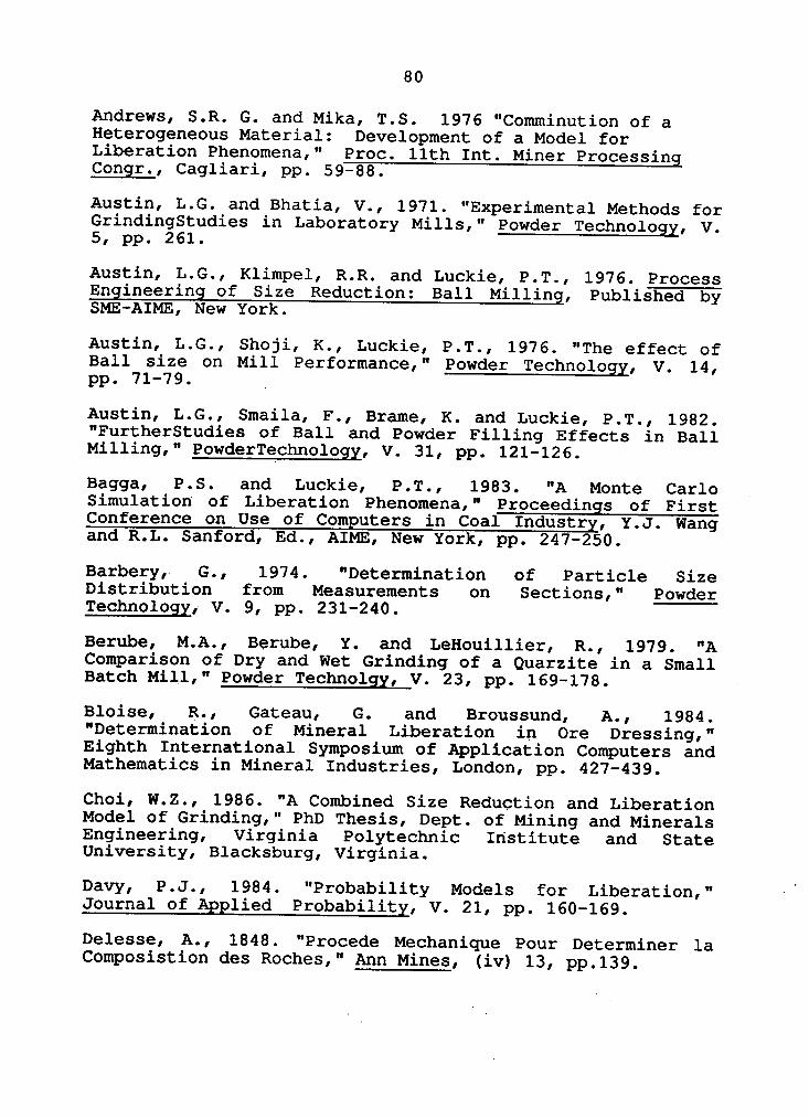
80

Andrews, S.R. G. and Mika, T.S. 1976 "Comminution of aHeterogeneous Material: Development of a Model forLiberation Phenomena," Proc. 11th Int. Miner ProcessingCongr., Cagliari, pp. 59-88.

Austin, L.G. and Bhatia, V., 1971. "Experimental Methods forGrindingStudies in Laboratory Mills," Powder Technology, V.5, pp. 261.

Austin, L.G., Klimpel, R.R. and Luckie, P.T., 1976. ProcessEngineering of Size Reduction: Ball Milling, Published bySME—AIME, New York.

Austin, L.G., Shoji, K., Luckie, P.T., 1976. "The effect ofBall size on Mill Performance," Powder Technology, V. 14,pp. 71-79. _

Austin, L.G., Smaila, F., Brame, K. and Luckie, P.T., 1982."FurtherStudies of Ball and Powder Filling Effects in BallMi1ling," PowderTechnology, V. 31, pp. 121-126.

Bagga, P.S. and Luckie, P.T., 1983. "A Monte Carlo _Simulation of Liberation Phenomena," Proceedings of FirstConference on Use of Computers in Coal Industry, Y.J. Wangand R.L. Sanford, Ed., AIME, New York, pp. 247-250.

Barbery,. G., 1974. "Determination of Particle SizeDistribution from Measurements on Sections," PowderTechnology, V. 9, pp. 231-240.

Berube, M.A., Berube, Y. and LeHouillier, R., 1979. "AComparison of Dry and Wet Grinding of a Quarzite in a SmallBatch Mill," Powder Technolgy, V. 23, pp. 169-178. ~

Bloise, R., Gateau, G. and Broussund, A., 1984."Determination of Mineral Liberation in Ore Dressing,"Eighth International Symposium of Application Computers andMathematics in Mineral Industries, London, pp. 427-439.

Choi, W.Z., 1986. "A Combined Size Reduction and LiberationModel of Grinding," PhD Thesis, Dept. of Mining and MineralsEngineering, Virginia Polytechnic Institute and StateUniversity, Blacksburg, Virginia.

Davy, P.J., 1984. "Probability Models for Liberation,"·‘

Journal of Applied Probability, V. 21, pp. 160-169.

Delesse, A., 1848. "Procede Nßchanique Pour Determiner laComposistion des Roches," Ann Mines, (iv) 13, pp.139.

81

Finlayson, R.M. and Hulbert, D.G., 1980. "The Simulation ofthe Behavior of Individual Minerals ixx a Closed GrindingCircuit," Proceeding, 3rd IFAC Symposium, Montreal, pp. 323-332.

Forssberg, E. and Zhai H., 1987. "Three DimensionalBehaviour of the Key Parameters Affecting Grinding in aBatch Ball Mill," Scandinavian Journal of Metallurgy, V. 15,pp. 53-56.

Fuerstenau, D.W. and Sullivan, D.A., 1962. "Analysis of theComminution of Mixtures in Ball Mills," Canadian Journal ofChemical Engineers, V. 40, pp. 43-50. -

Fuerstenau, D.W. and Sullivan, D.A., 1962. "SizeDistributions and Energy Consumption in Wet and DryGrinding," AIME Trans, V.220, pp. 379-402.

Gupta, V.K., Hodouin, D., Berube, M.A., and Everell, M.D.,1981. "The Estimation of Rate and Breakage Parameters From

~~ -Batch Grinding Data for a Complex Pyritic Ore Using Back-Calculation Method," Powder Technology, V.28, pp. 97-106.

Gupta, V.K. and Kapur, P.C., 1974. "Empirical Correlationsfor the Effects of Particulate Mass and Ball Size of theSelection Parameters in the Discretized Batch GrindingEquation," Powder Technology, V.10, pp. 217-223.

Gupta, V.K, Zouit, H. and Hodouin, D., 1985. "The Effect of ·Ball and Mill Diameters on Grinding Rate Parameters in DryGrinding Operation," Powder Technology, V.42, pp. 199-208.

Herbst, J.A. and Fuerstenau, D.W., 1968. "The Zero OrderA

Production of Fine Sizes in Comminution and Its Implicationsin Simulation." Trans. SME AIME, V.241, pp. 538-548.

Herbst, J.A. and Fuerstenau, D.W., 1972. "Influence of MillSpeed and Ball Loading on the Parameters of. the BatchGRinding Equation," Trans. SME AIME, V.252, pp. 169-176.

Herbst, J.A. and Fuerstenau, D.W., ”1973. "MathematicalSimulation of Dry Ball Milling Using Specific PowerInformation," Trans. SM AIME, V.254, pp. 343-348. ‘

Kelsall, D.F., Reid, K.J. and Restarick, C.J., 1968/1969."Continuous Grinding in a Small Wet Ball Mill Part II. AStudy of the Influence of Hold-Up Weight," Powder Technolgy,V.2 pp. 162-168. ·

82

Kuwahara, Y., 1971. "Experimental Study of SelectionFunction and Distribution Function," Journal of ChemicalEngineering, Japan, V.4 No.4, pp. 359-363.

King, R.P., 1978. "Determination of Particle SizeDistribution from Measurements on Sections," PowderTechnology, V.21, pp.147-150.“

King, R.P., 1979. "A Model for the Quantitative Estimationof Mineral Liberation by Grinding," International Journal ofMineral Processing, V.6, pp. 207-220.

King, R.P., 1982. "The Prediction of Mineral Liberation fromMineral Texture," XIV MPC, Toronto, Vlll 1.1-1.18.

Klimpel, R.R and Austin, L.G., 1983. "A Preliminary Model ofV Liberation from a Binary System," Powder Technology, V. 34,pp. 121-130.

Le Houillier, Van Neste, A. and Marchand, J.C., 1977.”influence of Charge on the Parameters of the Batch Grinding‘‘““ “

°Equation' and" Its Implications in Simulation," PowderTechnology, V.16, pp. 7-15.

Li, T.M., 1976. "The new Look at Asarco's Tennessee Mines,"Mining Engineering V.27, pp. 37-41.

Lin, C.L., 1986. "Measurement and Prediction of Mineral VLiberation During Grinding," Ph.D. Thesis, Dept. ofMetallurgy and Metallurgical Engineering, Univ. of Utah,Salt Lake City, Utah. ·

Lin, C.L., Miller, J.D. and Herbst, J.A., 1987 "Solutions tothe Transformation Equation for Volumetric GradeDistributions from Linear and/or Areal Grade Distributions,"Powder Technology V.50, pp. 55-63.

Lo, Y.C. and Herbst, J.A., 1986. "Consideration of Ball SizeEffects in the Population Balance Approach to Mill Scale-Up," in: Advances in Mineral Processing (P. Somasundaran,ed.), SME-AIME, Littleton, Colorado, pp. 33-47.

Lynch, A., Whiten, W. and Draper, N., 1967. "Developing the’

Optimum Performance of a Multi-Stage Grinding Circuit,"Trans. IM, V.76, pp. C169-C182.

Mankosa, M.J., Adel, G.T. and Yoon, R.H., 1986. "Effect ofMedia Size in Stirred Ball Mill Grinding of Coal," PowderTechnology, Vol. 49, pp. 75-82.

- 83

Miller, J.D. and Lin C.L., 1988. "Treatment of PolishedSection Data for Detailed Liberation Analyis," InternationalJournal of Mineral Processing, V.22, pp. 1-18.

Tangsathitkulchai, C. and Austin, L.G., 1985. "The effect ofSlurry Density on Breakage Parameters of Quartz, Coal andCopper Ore in Laboratory Ball Mill," Powder Technology,V.42, pp. 287-296.

Thompson, E., 1930. "Quantitative Microscope Analysis,"Journal of Geology, V.27, pp. 276.

Underwood, E.E., 1970. Quantitative Stereology, Addison-Wesley, Reading, Mass.

Wiegel, R.L. and Li, K., 1967. "A Random Model for MineralLiberation by Size Reduction," Trans. SME AIME, V.238, pp.179-189.

Yang, D., Mempel, G. and Fuerstenau, D.W., 1967. "ALaboratory Mill for Batch Grinding Experimentation," Tran.SM AIME, V.238, pp. 273-275. - -

APPENDIX I

Image Analysis Data

~A

84 ‘

i85

TABLE I-1. Sphalerite Distributions in 14x2O mesh forvarious grinding times at 40% critical speed.

ZnS Grinding, Time, minutesContent —---————-—----—-——---—--———-——————--—-—-—

(Wt%) 0.00 1.00 2.00 4.00

0-5 72.86 72.90 75.25 77.38

5-50 6.36 5.44 4.90 4.45

50-95 2.97 3.19 2.75 2.46

95-100 17.81 18.47 17.10 15.71

TABLE I-2. Sphalerite distributions in 14x20 mesh forA

various grinding times at 85% critical speed

ZnS °Grinding, Time, minutes

Content ——--——-——-·------------—----—-—--——-—-—(Wt%) 0.00 1.00 2.00 4.00

0-5 72.86 75.29 77.34 79.40

5-50 6.36 6.35 5.45 5.37

50-95 2.97 2.32 1.67 1.91

95-100 17.81 16.03 15.54 13.32

0é

86

TABLE I-3. Sphalerite distributions in 10x14 mesh forvarious grinding times with 3/4" ball size.

ZnS Grinding, Time, minutesContent ----—-————————-——--——----——————————-——

(Wt%) _ 0.00 1.00 2.00 4.00

0-5 82.79 81.11 85.72 87.93

5-50 7.08 7.69 5.50I

5.51

50-95 2.33 2.60 2.53 1.87

95-100 7.79 8.60 6.25 4.70

TABLE I-4. Sphalerite distributions in 10x14 mesh forvarious grinding times with

1”ball size.

ZnS Grinding, Time, minutesContent -—-——-—-—---------—-—-—--———--—----——(Wt%) 0.00* 0.00** 1.00 2.00 4.00

0-5 70.23 82.79 79.34 83.97 88.27

5-50 6.10 7.08 7.45 5.44 5.60

50-95 4.53u

2.33 3.34 3.44 1.65

95-100 19.13 7.79 9.87 7.15 4.47

* Feed used for 1 and 2 min grinding times.**Feed used for 4 min grinding time

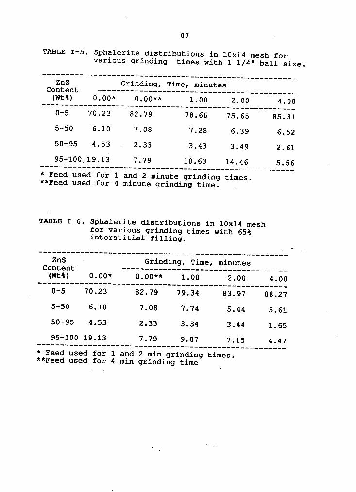
87

TABLE I-5. Sphalerite distributions in 10x14 mesh forvarious grinding times with l 1/4" ball size.

ZnS Grinding, Time, minutesContent —--—-—---—————-—-——----—-—----—-————-——————

(Wt%) 0.00* 0.00** 1.00 2.00 4.000-5 70.23 82.79 78.66 75.65 85.315-50 6.10 7.08 7.28 6.39 6.5250-95 4.53 _ 2.33 3.43 3.49 2.61

95—100_19.13 7.79 10.63 14.46 5.56 4

* Feed used for 1 and 2 minute grinding times.**Feed used for 4 minute grinding time. _

TABLE I-6. Sphalerite distributions in 10x14 meshfor various grinding times with 65%interstitial filling.

ZnS Grinding, Time, minutesContent -—--——-—--—-—--—--—-———-—-—-—-——-—-—

(Wt%) 0.00* 0.00** 1.00 2.00 4.00

0-5 70.23 82.79 79.34 83.97 88.27

5-50 6.10 7.08 7.74 5.44 5.61 ·50-95 4.53 2.33 3.34 3.44 1.65

95-100 19.13 7.79 9.87 7.15 4.47

* Feed used for 1 and 2 min grinding times.**Feed used for 4 min grinding time

·

88

TABLE I-7. Sphalerite distributions in 10x14 mesh for .various grinding times with 100% interstitialfilling.

ZnS Grinding, Time, minutesContent —---—-—---—-——-—-—-—-—--————-——————————

(Wt%) 0.00 4.00

0-5 82.33 86.22

5-50 5.70 5.11

50-95 2.88 2.27

95-100‘ 9.09 6.39

TABLE I—8. Sphalerite distributions in 10x14 mesh for ‘various grinding times with 150% interstitialfilling.-

ZnS Grinding, Time, minutesContent ---------—---------—-—-------—-—----——--(Wt%) 0.00 4.00

0-5 _ 82.33 80.279

5-50 5.70 6.77

50-95 2.88 4.20

95-100 9.09 8.76

89

TABLE I-9. Sphalerite distributions in 14x2O mesh forvarious grinding times with 1" ball size (dry).

ZnS Grinding, Time, minutesContent --——-—————--—-—-----——-—————-————-————-———(Wt%) 0.00 4.000-5 75.39 78.525-50 5.02 4.9450-95 3.35 2.9695-100 16.24 13.58

TABLE I-10. Sphalerite distributions in 14x2O mesh for Ivarious grinding times with 1 in" balls and70% solids.

ZnS Grinding, Time, minutesContent -------—-—-----—----—--—-------—---—-———(Wt%) 0.00 1.00 2.00 4.000-5 ° 75.39 70.67 77.43 81.93 I

5-50 5.02 4.39 4.50· 3.9250-95 3.35 3.59 4.36 2.7095-100 16.24 21.35 13.71 11.44

‘I

APPENDIX II

Percent Remaining Values for the- Disappearance Plots

91

TABLE II-1. Percent remaining of original 14x20feed for various grinding times at 40%

· critical speed.

ZnS Grinding, Time, minutesContent -—-————-——-—--—-—---————————-—-—-————

(Wt%) 0.00 1.00 2.00 4.00 .

0-5 100.00 80.07 66.08 44.39

5-50 100.00 68.47 49.20 29.24

50-95 100.00 85.96 59.25 34.62

95-100 100.00 83.00 61.37 36.87

TABLE II-2. Percent remaining of original 14x20 feedfor various grinding times at 85% criticalspeed.

ZnS Grinding, Time, minutesContent --—------------—------—-------———-—--—-

(Wt%) 0.00 1.00 2.00 4.00

0-5 100.00 66.39 44.65 22.08

5-50 100.00 64.14 36.05 17.11

50-95 100.00 50.18 23.65 13.05

95-100 100.00 57.82 36.70 15.15W

92

TABLE II-3. Percent remaining of original 10x14 feed forvarious grinding times with 3/4" ball size.

ZnS Grinding, Time, minutesContent —-———-——————————————————————--—--——-——

(Wt%) 0.00 1.00 2.00 4.00A

0-5 _ 100.00 65.11 46.71 22.62 .

5-50 100.00 72.21 35.07 16.56

50-95 100.00 74.19 48.94I

17.07

95-100 100.00 73.34 I 36.18 12.85

· “ ‘ TABLE II-4. Percent remaining of origninal 10x14 feedfor various grinding times with l" ballsize.

ZnS Grinding, Time, minutes_ Content -------———-—----—-—---------——--—-———

(Wt%) 0.00 1.00 2.00 4.00

0-5 100.00 75.19 50.53 18.85

5-50 100.00 84.45 37.68 ·14.01

50-95 100.00 49.02 32.06 12.52

95-100 100.00 34.33 15.78 10.15

93u

TABLE II—5. Percentremaining of original 10x14 feedfor various grinding times with 1 1/4" ballsize.

ZnS Grinding, Time, minutesContent ---—--—-——--—--——————--—---———--————————-

(Wt%) 0.00 1.00 2.00 4.00

0-5 100.00 74.23 40.34 17.98

5-50 100.00 79.30 39.23 16.08

50-95 100.00 50.26 28.82 19.54

95-100 100.00 36.92 28.30 12.45

0TABLE II-6. Percent remaining of original 10x14 feed for

various grinding times at 65% interstitialfilling.

ZnS Grinding, Time, minutesContent —--————-—--—----—-——-—-----————----—-———

(Wt%) · 0.00 1.00 2.00 4.00

0-5 100.00 75.19 50.53 18.850

5-50 100.00 84.45 37.68 14.01

50-95 100.00 49.02 32.06 12.52

95-100· 100.00 34.33 15.78 10.15

A 94

TABLE II-7. Percent remaining of original 10x14 feed forvarious grinding times with 100% interstitialfilling.

ZnS Grinding, Time, minutesContent -------————-—-——---——---————-——-——————

(Wt%) 0.00 4.00

0-5 100.00 28.09

5-50 100.00 24.06

50-95 100.00 21.16

95-100 100.00 18.85

TABLE II—8. Percent remaining of original 10x14 feedfor various grinding times with 150%interstitial filling. ·

ZnS Grinding, Time, minutesContent --—---————---—----——--—-—-——-—-—----—-—

(Wt%) ~ 0.00 4.00

0-5 100.00 45.788

5-50 100.00 55.77

50-95 100.00 68.47

95-100 100.00 45.25

95

TABLE 11-9 Percent remaining of original 14x20 feedfor various grinding times with 1" balls(dry).

ZnS Grinding, Time, minutesContent --—-—--————--—---——-——-——-————-————————

(Wt%) 0.00 4.00

0-5 100.00 16.68

5-50 100.00 15.77

50-95 100.00 14.14

95-100 100.00 13.40

TABLE II—10.Percent remaining of original 14x20 feedfor various grinding times with l" ballsand 70% solids.

ZnS Grinding, Time, minutesContent —---—--------—----—--—---—--——-——————-——

(Wt%) 0.00 1.00 2.00 4.00

0-5 100.00 55.21 35.01 9.95 _

5-50 100.00 51.51 30.55 7.15

50-95 100.00‘

63.12 44.36° 7.37

95-100 100.00 77.43 28.78 6.45

APPENDIX III

DiS&pp€a.I‘&I1C€ Plots

l96

97

10 _

¤0*E ·E0

g 10OC 1

-1-¤CQ)O 0 0-5x SPHAL

0. ¤ 6-60z SPHA1.A 50-9556 SPHAL*< 95-100x SPHAL __

*0 1 2 3 9 4 6Time (mm)

Figure III—1 Disappearance plot for a 14x2O mesh feed at40% critical speed.

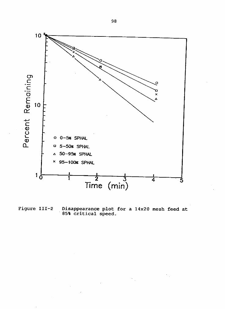
9810

Bx, \o·

EO x

E AQ) 10

CK .-+-4C

- (D

o 0-sz SPHAL0. ¤ 6-soz SPHALA‘ 50-95S SPHAL

" 95-1005 SPHAL1 •

1 • 2 • 4 . 5Tnme (mm) 1

Figure III—2 Disappearance plot for a 14x2O mesh feedat-

° 85% critical speed.

99

10 _

6

OlE 0

.E éO

·

-4-/ · n

CQ)

GL; o 0-6;; SPHALQ. ¤ 6-60;; spam.

A 50-9558 SPHAL*‘

95-100z SPHAL

*0 12 _ 3 4 5'Üme (mm)

Figure III—3 Disappearance plot: for a 10xl4 mesh feed witha 3/4" ball size.

100

10¤

A O

X ¤A

G7EC O‘*

XÜ

¤E Aq) 10 ><

CK4-*C0.)O 1 „ä 0 0-5% SPHAL

CL ¤ 6-60; SPHA1.A 50-95% SPHAL -U" 95-100% SPHAL

1 ' 1I 1· • 3 4, . 5Tume (mm)

Figure III- le Disappearance plot for a lOx14 mesh feed witha l" ball size.

101

10F 8

^

X Q

xO1EQ 8

OE xQ) 10

Of•+—*

° CQ)Q M .0 0-5:6 SPHAL

0_ _¤__ 6-soz ·sPHALA 50-95% SPHAL

" 95-100% SPHAL

1 •1 2 · 51 ‘ Time (min)

Figure III--5 Disappearance plot for a 10$c1_4 mesh feed witha 1 1/4" ball size.

102

10 0CI•

A G .

DxA

E•- . · xO ¤E A(D 10 °‘(lf

-4-·'CQ) .O

0 0-5ss SPHAL -Q. ¤ s—so¤ SPHAL

A 50-95% SPHAL ->< 95-100% SPHAL

Tume (mm)

Figure III—6 Disappearance plot for a 10xl4 mesh feed witha 65% interstitial filling.

103

10

OO-}¤

C A

O

(D 10CK

-4-*C(DOE

0 0-516 $PHAL0. ¤ 6-6016 61>1~1A1. '

A 50-95%, SPHAL°‘

95*.100:6 SPHAL

*0 1 2 3 4 1 6'Üme (mm) 1 3

Figure III—7 Disappearance plot for a 10xl4 mesh feed witha 65% interstitial filling.

‘

104

10 — 0

A

Cl· ”

0

C)E-'Z<E

Agg 10

I--ZL1.!O95 0 0-6;: s1=>HAa.0.. ¤ 6-60;: s1>HAL

A 50-95% SPHAL

>< 95-100;: SPHAI.

*0 1 4 2 ( ä 4 9 6

Figure III—8 Disappearance plot for a 10x14 mesh feed witha 150% interstitial filling.

105

10 · -x

X

A8

A0

CDC

EU

q) 10 0CK

é-6-JC(DO 0 O—5ss SPHAL

O. ¤ 6-soz spam.A 50-95:8 SPHAL*‘

95-100x SPHAL

Tume (mm)

Figure III- 9 Disappearance plot for a l4x20 mesh feed witha 70% solids grinding environment.

106

10

UVEE 9O e

(D 10OC-4-*C

-

O 0 0-5% SPHALC1. ¤ 6-60;; SPHAL

A 50--95% SPHAL*‘

95-100% SPHAL

g 10 1 2 6 4 6Time (mm)

Figure III- 10· Disappearance plot for a 14x20 mesh feed witha 100% solids grinding environment.

APPENDIX IV

Breakage and Energy Specific Breakage Rates

I107

l ‘

108

TABLE IV-1. Breakage and Specific Breakage Rates forRPM parameter in terms of percent criticalspeed.

Breakage Rate Specific Breakage RateZnS (1/min) (Tons/Kwhr)

Content -------------—----—————----——-—--—-—-------(Wt%) 40 85 40 85

0-5 .202 .403 .651 .738

5-50 .355 .441 1.145 .815

50-95 .265 .721 .857 1.319

l 95-100· .249 .548 .806 1.002

TABLE IV—2. Breakage and Specific Breakage Rates for ballsize parameter in terms of ball size in inches.

ZnSI

Breakage Rate Specific Breakage RateA

(1/min) ' (Tons/Kwhr)Content —-------—--------------—-----—-------------

. (Wt%) 3/4 1_ 1 1/4 3/4 1 1 l/4

0-5 .372 .424 .429 .676 .767 .819

5-50 .464 .491 .457 .845 .889 .873

50-95 .357 .713 .688 .650 1.290 1.314

95-100 .513 1.068 .996 .933 1.934 1.903

109

TABLE IV-3. Breakage and Specific Breakage Rates for millcharge parameter in terms of percentinterstitial filling.

Breakage Rate Specific Breakage RateZnS (1.min.) (Tons/Kwhr)

Content ---—--------—-———---———-—----------—-------(Wt%) 65 100 150 65 100 150

0-5 .424 .317 .195 .767 .905 .848

5-50 .491 .356 .145 .889 1.015 .629

Ä 50-95 .713 .388 .095 1.290 1.107 .411// 95-100 1.069 .417 .198 1.934 1.189 .860

TABLE IV-4. Breakage and Specific Breakage Rates for wet° grinding parameter in terms of percent solids.

Breakage Rate Specific Breakage RateZnS (1/min) (Tons/Kwhr)

Content -----—-------————-—---—--------—-—---------(Wt%) 100 70* 100 70*

0-5 .448 .577 .810 1.039

5-50 .462 .660 .836 1.187 ·

50-95 .489 .652 .885 1.173

95-100 .502 .686 .909V

1.234

* Four minute grind values used for calculations.

APPENDIX V

Chemical Assay Procedure

//

Ü ‘ 110U

111

ASSAY PROCEDURE: Samples of narrowly sized material were

split into representative fractions of approximately 10

grams. A mechanical mortor and pestle was used for a period

of 15 minutes to pulverize the specimens. Once pulverized,

.5 grams were put into a 500 ml beaker. Twenty· ml of

concentrated hydrochloric acid was then added to the beaker,

and allowed to digest the sample for approximately 10i

minutes while heating the solution. Ten ml of concentrated

/ nitric acid was then added to the beaker and digestion

continued for 10 more minutes. The beaker was then allowed

to cool and the solution was transferred to a 500 ml

volumetric flask and made up to volume with distilled water.

The solution was then filtered through a Whatman #1

filter paper into a clean, dry 100 ml beaker and atomized

through a Spectraspan IV Plasma Emission Spectrometer. The

wave length used to detect zinc was 206.2 nm. Standards for

calibration were made from a 1000 mg/l Fisher Scientific

stock solution.