the economic value of co-movement between oil price and exchange rate using copula-based garch...

Energy Economics 34 (2012) 270–282

Contents lists available at ScienceDirect

Energy Economics

j ourna l homepage: www.e lsev ie r.com/ locate /eneco

The economic value of co-movement between oil price and exchange rate usingcopula-based GARCH models☆

Chih-Chiang Wu a,⁎, Huimin Chung b, Yu-Hsien Chang b

a Discipline of Finance, College of Management, Yuan Ze University, 135 Yuan-Tung Road, Chungli, Taoyuan, Taiwanb Graduate Institute of Finance, National Chiao Tung University, Hsinchu, Taiwan

☆ This research is partially supported by a grant fromTaiwan (NSC98-2410-H-155-026).⁎ Corresponding author. Tel.: +886 3 4638800 3661;

E-mail address: [email protected] (C.-C1 The relationship between oil and stock markets mi

issue in terms of energy market investigations; howefurther theoretical foundations and is beyond theTherefore, this study concentrates on the discussion andbetween oil and exchange-rate markets, and the issue oand stock markets is left for future research.

0140-9883/$ – see front matter © 2011 Elsevier B.V. Adoi:10.1016/j.eneco.2011.07.007

a b s t r a c t
a r t i c l e i n f o
Article history:Received 2 September 2010Received in revised form 11 July 2011Accepted 16 July 2011Available online 22 July 2011

JEL classification:C52C53G11Q43Q47

Keywords:OilExchange rateCo-movementTime-varying copulaEconomic value

The US dollar is used as the primary currency of international crude oil trading; as such, the recent substantialdepreciation in the US dollar has resulted in a corresponding increase in crude oil prices. In addition, oil priceand exchange-rate returns have been shown to be skewed and leptokurtic, and to exhibit an asymmetric ortail dependence structure. Therefore, this study proposes dynamic copula-based GARCH models to explorethe dependence structure between the oil price and the US dollar exchange rate. More importantly, an asset-allocation strategy is implemented to evaluate economic value and confirm the efficiency of the copula-basedGARCH models. In terms of out-of-sample forecasting performance, a dynamic strategy based on the CGARCHmodel with the Student-t copula exhibits greater economic benefits than static and other dynamic strategies.In addition, the positive feedback trading activities are statistically significant within the oil market, but thisinformation does not enhance the economic benefits from the perspective of an asset-allocation decision.Finally, a more risk-averse investor generates a higher fee for switching from a static strategy to a dynamicstrategy based on copula-based GARCH models.

the National Science Council of

fax: +886 3 4354624.. Wu).

ght also represent a pertinentver, this needs to rely on thescope of the current study.evaluation of the relationshipf the relationship between oil

2 The US Dollar InEuro (57.6%), JapanSwedish Krona (4.2%

ll rights reserved.

© 2011 Elsevier B.V. All rights reserved.

1. Introduction

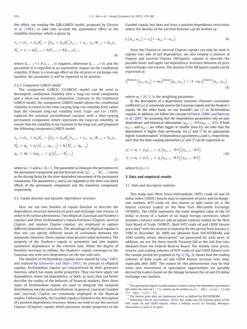
Energy commodities differ from other trading products both intheir uniqueness and their non-renewable nature. Due to the lownumber of oil-producing countries, most countries must rely onenergy imports. As a result, the prices of energy commodities havebeen profoundly influenced by numerous factors, such as governmentpolicy, geopolitics, seasonal aspects, military conflicts, demand andsupply. In particular, since the US dollar is commonly used as theinvoicing currency in the international energy commodity market,changes in the value of the US dollar have knock-on effects onfluctuations of commodity prices and in turn affect the economicactions of energy commodity importing and exporting countries.1 In

addition, over the last few years, energy commodity prices haveexperienced an unprecedented high level of fluctuations. For example,the crude oil price rose steadily from $20 per barrel in January 2002 toa high of $147 per barrel in July 2008. It then fell sharply to $32 perbarrel in January 2009. In the meantime, since 2002 the US dollarindex (USDX2) has behaved in a markedly different manner to theway it behaved prior to 2002 in that it has tended to move in theopposite direction to the price of crude oil. As such, while the crude oilprice has soared, the US dollar has depreciated to a historically lowprice, and vice versa. This negative relationship has resulted indiversification and hedging benefits between crude oil commoditiesand the US dollar. As a result, accuratemodeling and forecasting of thevolatility and dependence structures of oil and exchange-rate returnsare of considerable interest to global energy-related researchers,financial institutions, and investors.

In recent years, a number of methods have been employed toexplore the relationship between oil prices and the US dollarexchange rate. For example, using Hansen's GMM model, Yousefi

dex (USDX®) is an average of six major world exchange rates: theese Yen (13.6%), UK Pound (11.9%), Canadian Dollar (9.1%),) and Swiss Franc (3.6%).

http://dx.doi.org/10.1016/j.eneco.2011.07.007

mailto:[email protected]

http://dx.doi.org/10.1016/j.eneco.2011.07.007

http://www.sciencedirect.com/science/journal/01409883

271C.-C. Wu et al. / Energy Economics 34 (2012) 270–282

andWirjanto (2004) investigated the impact of fluctuations in the USdollar exchange rate on the formation of OPEC3 and verified that thecorrelation of oil prices and the US dollar exchange rate is negative.Akram (2004) presented evidence of a non-linear negative relation-ship between oil prices and the Norwegian exchange rate, and pointedout that the nature of the relationship varies with the level and trendin oil prices. Cifarelli and Paladino (2010) used a multivariate CCCGARCH-M model to determine that oil price dynamics are associatedwith exchange rate behavior, and found strong evidence that oil priceshifts are negatively related to exchange rate changes.

Further, additional studies have focused on discussing the lead–lag relationship between oil prices and the exchange rate, as well astheir interactive influence. For example, Krichene (2005) used thevector error correction model (VECM) to demonstrate that thenegative impact of the falling nominal effective exchange rate couldlead to a surge in oil prices, and inversely either long-term or short-term effects. Sari et al. (2009) employed generalized forecast errorvariance decompositions and generalized impulse response func-tions to find evidence of a weak long-run equilibrium relationshipbut with strong feedback in the short run. Lizardo andMollick (2010)used the cointegration analysis to reveal that oil prices significantlycontribute to the explanation of movements in the value of the USdollar in the long-run: an increase in the real price of oil leads to asignificant depreciation of the US dollar relative to net oil exportercountries. While these studies differ from the current study in termsof the ultimate purpose, they still support the negative relationshipbetween oil prices and the exchange rate.

The majority of the existing literature points out the negativerelationship between crude oil prices and the US dollar exchange rate.A number of possible explanations for this negative relationship aresummarized as follows. First, oil-exporting countries want to stabilizethe purchasing power of their export revenues (US dollar) in terms oftheir imports (non-US dollar), so in order to avoid losses they mayadopt currencies pegged to the US dollar. Second, the depreciation ofthe US dollar makes oil cheaper for consumers in non-US dollarregions, thereby changing their crude oil demand, which eventuallycauses adjustments in the oil price as it is denominated in US dollars.Third, a falling US dollar reduces the returns on US dollar-denominated financial assets, increasing the attractiveness of oil andother commodities to foreign investors. Commodity assets are alsoregarded as a hedge against inflation, since US dollar depreciationincreases the risk of inflationary pressures in the United States. Basedon the above reasons, we must consider changes in the exchange rateand the oil price simultaneously.

The analysis of financial marketmovements and co-movements isimportant for effective diversification in portfolio management.Previous research, such as Bekiros and Diks (2008), and Chang et al.(forthcoming), has commonly used multivariate GARCH models as ameans of estimating time-varying dependence structures, but this isoften based on severe restrictions in order to guarantee a well-defined covariance matrix. In addition, the VAR model and multi-variate GARCH models assume that the asset returns follow amultivariate normal or Student-t distribution with linear depen-dence. This assumption is at odds with numerous empirical researchstudies, which show that oil and exchange-rate returns are skewed,leptokurtic and fat-tailed, following very dissimilar marginal distri-butions as well as different degrees of freedom parameters.4 Further,the actual relationship between oil prices and the exchange rate ispossibly non-linear or asymmetrical. For example, crude oil returnsappear to bemore negatively associated with US dollar returns when

3 The Organization of the Petroleum Exporting Countries is a cartel of twelvecountries. The principal goals are safeguarding the cartel's interests and securing asteady income to the producing countries.

4 Examples include Giot and Laurent (2003), Patton (2006), and Fan et al. (2008).

the US dollar depreciates as compared to when the US dollarappreciates, especially after 2002. Thus, the linear correlation mayfail to capture the potentially asymmetric dependence between oiland exchange-rate returns.

To address these drawbacks, we use copula-based GARCHmodels tocapture the volatility and dependence structures of crude oil andexchange-rate returns. The copula-based GARCH models allow forbetterflexibility in joint distributions than bivariate normal or Student-tdistributions. In addition, employing the heterogeneous agent model,Sentana and Wadhwani (1992) categorized investors into rational (i.e.expected utility maximizers) and positive feedback (i.e. trend chasing)investors and proposed a modified CAPM. By examining the role ofpositive feedback trading in the US stock market, they discovered thatduring lowvolatility periods, stock returns are positively autocorrelated,but during high volatility periods they tend to be negatively auto-correlated. Sucha reversal relationship in stock return autocorrelation isconsistent with the notion that some traders pursue positive feedbackstrategies, i.e. they buy (sell) when the price rises (falls). Recently,Cifarelli and Paladino (2010) employed this modified CAPM toinvestigate speculative behavior in the oil market, where theydiscovered evidence of positive feedback trading activities. Thus, thecurrent study assumes that the impact of feedback trading activitieswill influence the dynamic behavior of oil prices. Moreover, threetypes of marginal models are employed to capture a variety ofcharacteristics of oil and exchange-rate volatility processes, includ-ing volatility clustering, the leverage effect, and the long-run effect.Five types of copula functions are also used to provide amore generaldependence structure, as opposed to treating it as simple linearcorrelation.

Furthermore, if a model performs better statistically this does notnecessarily imply that the model performs well in practice; as such,we follow Fleming et al. (2001, 2003) in evaluating the out-of-sampleforecast performance based on the copula-based GARCH modelsthrough the use of a strategic asset-allocation problem. We also takethe transaction cost problem into consideration and compute thebreak-even transaction cost, as discussed in Han (2006): based on therelationship between the break-even cost and the real transactioncost, an investor decides whether or not to trade.

Our contribution to the literature is twofold. First, we propose thecopula-based GARCH models to elastically describe the volatility anddependence structure of oil price and US dollar exchange-rate returns.The copula-based GARCH models can be used to capture the potentialskewness and leptokurtosis of oil and exchange-rate returns, as well asthe possibly asymmetric and tail dependencebetweenoil and exchange-rate returns. We find that the symmetric copulas seem superior to theasymmetric copulas in terms of the description of a dependencestructure between crude oil and exchange-rate returns, and the CGARCHmodelwith theGaussian copula exhibits a better explanatory ability.Wealso observe that the dependence structure between crude oil and USdollar exchange-rate returns is not very significant before 2003, but itbecomes negative and descends continuously after 2003. Second, ratherthan using statistical criteria, we examine whether the copula-basedGARCH models can benefit an investor by implementing an asset-allocation strategy. In terms of out-of-sample results, we find that thedynamic strategies based on the copula-based GARCH models outper-form the static strategy and other dynamic strategies based on the CCCGARCH and DCC GARCH models; this demonstrates that skewness andleptokurtosis of crude oil and USDX futures returns are economicallysignificant. Furthermore, the CGARCH model with the Student-t copulayields the highest performance fees and break-even transaction costs toattract investors to switch their trading strategy. In addition, positivefeedback trading activities are statistically significant in the crude oilmarket, but this feedback trading information does not enhanceinvestors' economic benefits. Finally, more risk-averse investors arewilling to pay higher fees to switch from a static strategy to a dynamicstrategy based on copula-based GARCH models.

Gaussian copula with Normal marginal

N(0,1)

N(0

,1)

0.02

0.04

0.06

0.08

0.1

0.12

0.14

0.16

Gaussian copula with Skewed-t marginal

Skewed-t(5,-0.1)

Ske

wed

-t(5

,-0.

1)

0.02

0.04

0.060.08

0.10.12

0.140.16

0.18

0.2

0.22

-2 -1 0 1 2 -2 -1 0 1 2

N(0,1) Skewed-t(5,-0.1)-2 -1 0 1 2 -2 -1 0 1 2

N(0,1) Skewed-t(5,-0.1)-2 -1 0 1 2 -2 -1 0 1 2

N(0,1) Skewed-t(5,-0.1)-2 -1 0 1 2 -2 -1 0 1 2

Student-t copula with Normal marginal

N(0

,1)

0.02

0.04

0.06

0.08

0.1

0.12 0.14

0.16

Student-t copula with Skewed-t marginal

Ske

wed

-t(5

,-0.

1)

0.02

0.04

0.06 0.08

0.10.12

0.140.16

0.180.22

0.24

Clayton copula with Normal marginal

N(0

,1)

0.02

0.04

0.06

0.08

0.1

0.12

0.14

Clayton copula with Skewed-t marginal

Ske

wed

-t(5

,-0.

1)

0.02

0.04

0.06

0.08

0.1 0.12

0.14 0.16

0.18 0.2

Survival Clayton copula with Normal marginal

N(0

,1)

0.02

0.04

0.06

0.08

0.1

0.12

0.14

Survival Clayton copula with Skewed-t marginal

Ske

wed

-t(5

,-0.

1)

0.02

0.04

0.06

0.080.1

0.12

0.14

0.160.18

0.2

-2-1

01

2-2

-10

12

-2-1

01

2-2

-10

12

-2-1

01

2-2

-10

12

-2-1

01

2-2

-10

12

a

b

c

d

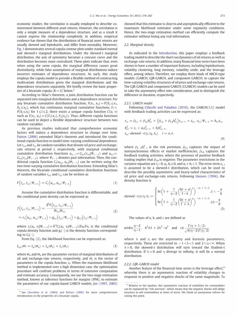
Fig. 1. Contour plot based on a. Gaussian copula, b. Student-t(5) copula, c. Clayton copula, and d. survival Clayton under the dependence parameter, τ=−0.2, with two types ofmarginal distributions (Normal (0, 1) and Skewed-t (5,−0.1)).

272 C.-C. Wu et al. / Energy Economics 34 (2012) 270–282

The remainder of this paper is organized as follows. In the nextsection, we introduce the copula-based GARCH models in detail.Section 3 presents the empirical estimation results. Section 4 in-troduces an economic evaluation methodology and provides theresults for the out-of-sample forecasts of the copula-based GARCHmodels. Finally, Section 5 offers conclusions.

2. Econometric model

2.1. Time-varying copula

In the past, multivariate normal distributions have been used todescribe multiple asset returns across a broad range of financial and

6 Relative to the equities, this asymmetric reaction of volatilities for commodities


economic studies; the correlation is usually employed to describe co-movement between different asset returns. However, the correlation isonly a simple measure of a dependence structure, and as a result itcannot express the relationship completely. In addition, empiricalevidence has shown that the distributions of financial asset returns areusually skewed and leptokurtic, and differ from normality. Moreover,Fig. 1 demonstrates several copula contour plots under standard normaland skewed-t marginal distributions. Under the skewed-t marginaldistribution, the axis of symmetry becomes a concave curve and thedistribution becomes more centralized. These plots indicate that, evenwhen using the same copula, the marginal difference causes greatdissimilarity, while false assumptions of marginal distributions induceincorrect estimates of dependence structures. As such, this studyemploys the copula model to provide a flexible method of constructingmultivariate distributions given the marginal distributions and thedependence structures separately. We briefly review the basic proper-ties of a bivariate copula (K=2) below.5

According to Sklar's theorem, a joint distribution function can beseparated into marginal distributions and a dependence structure. Forany bivariate cumulative distribution function, F(x1, x2)=P(X1≤x1,X2≤x2), which has continuous marginal cumulative functions, Fi=P(Xi≤xi) for 1≤ i≤2, there exists a unique copula function C(u, v)such as F(x1, x2)=C(F1(x1), F2(x2)). Thus, different copula functionscan be used to depict a flexible dependence structure between tworandom variables.

As previous studies indicated that comprehensive economicfactors will induce a dependence structure to change over time,Patton (2006) extended Sklar's theorem and introduced the condi-tional copula function tomodel time-varying conditional dependence.Let ro,t and re,t be random variables that denote oil price and exchange-rate returns at period t, respectively, with marginal conditionalcumulative distribution functions uo, t=Go,t(ro,t|Ψt− 1) and ue,t=Ge,t(re,t|Ψt−1), where Ψt−1 denotes past information. Then, the con-ditional copula function Ct(uo,t, ue,t|Ψt−1) can be written using thetwo time-varying cumulative distribution functions. Extending Sklar'stheorem, the bivariate conditional cumulative distribution functionsof random variables ro,t and re,t can be written as

F ro;t ; re;t jΨt−1

� �= Ct uo;t ;ue;t jΨt−1

� �ð1Þ

Assume the cumulative distribution function is differentiable, andthe conditional joint density can be expressed as

f ro;t ; re;t jΨt−1

� �=

∂2F ro;t ; re;t jΨt−1

� �∂ro;t∂re;t

= ct uo;t ;ue;t jΨt−1

� �× go;t ro;t jΨt−1

� �× ge;t re;t jΨt−1

� � ð2Þ

where ct(ut, vt|Ψt−1)=∂ 2Ct(ut, vt|Ψt−1)/∂ut∂vt is the conditionalcopula density function and gi(·) is the density function correspond-ing to Gi(·).

From Eq. (2), the likelihood function can be expressed as:

Lo;e Θð Þ = Lo Θoð Þ + Le Θeð Þ + Lc Θcð Þ; ð3Þ

whereΘo andΘe are the parameter vectors of marginal distributions ofoil and exchange-rate returns, respectively, and Θc is the vector ofparameters in the copula function, ct. When the maximum likelihoodmethod is implemented over a high dimension case, the optimizationprocedure will confront problems in terms of extensive computationand estimate accuracy. Consequently, we use the two-stage estimationmethod, known as inference functions for margins (IFM), to estimatethe parameters of our copula-based GARCH models. Joe (1997, 2005)

5 See Cherubini et al. (2004) and Nelsen (2006) for more comprehensiveintroductions to the properties of a bivariate copula.

showed that this estimator is close to and asymptotically efficient to themaximum likelihood estimator under some regularity conditions.Hence, the two-stage estimation method can efficiently compute theestimator without losing any real information.

2.2. Marginal density

As indicated in the Introduction, this paper employs a feedbacktradingmodel to describe the short rundynamicsof oil returns aswell asexchange-rate returns. In addition,manyfinancial time series have beenshown to have a number of important features, including leptokurtosis,volatility clustering, long memory, volatility smile, and the leverageeffect, among others. Therefore, we employ three kinds of ARCH-typemodels (GARCH, GJR-GARCH, and component GARCH) to capture thetime-varying volatility structures of oil price and exchange-rate returns.The GJR-GARCH and component GARCH (CGARCH)models can be usedto take the asymmetry effect into consideration, and to distinguish thedifference in duration, respectively.

2.2.1. GARCH modelFollowing Cifarelli and Paladino (2010), the GARCH(1,1) model

with feedback trading activities can be expressed as:

ri;t = βi;1 + βi;2h2i;t + βi;3 + βi;4h

2i;t

� �ri;t−1 + εi;t ; εi:t jΨt−1 = hi:tzi:t ;

h2i;t = ci + aiε2i;t−1 + bih

2i;t−1;

zi:teskewed−t zi jηi;λið Þ; i = o; e;

ð4Þ

where βi, 2hi, t2 is the risk premium, βi,3 captures the impact of

nonsynchronous effects or market inefficiencies, βi,4 captures thefeedback trading activities, where the presence of positive feedbacktrading implies that βi,4 is negative. The parameter restrictions in thevariance equation are ciN0, ai, bi≥0, and ai+bi<1. The error term εi, tis assumed to be a skewed-t distribution, which can be used todescribe the possibly asymmetric and heavy-tailed characteristics ofoil price and exchange-rate returns. Following Hansen (1994), thedensity function is

skewed−t z jη;λð Þ =bc 1 +

1η−2

bz + a1−λ

� �2� �− η + 1ð Þ=2; z < − a

b

bc 1 +1

η−2bz + a1 + λ

� �2� �− η + 1ð Þ=2; z≥− a

b

8>>>><>>>>:ð5Þ

The values of a, b, and c are defined as

a≡4λcη−2η−1

; b2≡1 + 2λ2−a2 and c≡ Γ η + 1= 2ð Þffiffiffiffiffiffiffiffiffiffiffiffiffiffiffiffiffiffiffiffiffiffiffiffiffiffiffiffiffiffiffiffiffiπ η−2ð ÞΓ η = 2ð Þp

where λ and η are the asymmetry and kurtosis parameters,respectively. These are restricted to −1<λ<1 and 2<η<∞. Whenλ=0, the skewed-t distribution will turn toward the Student-tdistribution. If λ=0 and η diverge to infinity, it will be a normaldistribution.

2.2.2. GJR–GARCH modelAnother feature of the financial time series is the leverage effect,6

whereby there is an asymmetric reaction of volatility changes inresponse to positive and negative shocks of the same magnitude. To

can be explained by “risk aversion”, which means that the negative shocks will obligeinvestors to sell commodities at times of stress. We thank an anonymous referee forraising this point.

7 The appropriate logistic transformation is used to ensure the dependence parametersfall within the interval (−1,1), which can be written as ρt⁎=−ln[(1−ρt)/(ρt+1)] andτt⁎=− ln[(1−τt)/(τt+1)].

8 The futures price data are continuous series, as defined by DATASTREAM.9 Following Cifarelli and Paladino (2010), this study uses the Tuesday prices of the

WTI crude oil and USDX futures; when a holiday occurs on Tuesday, Monday'sobservation is used in its place.


this effect, we employ the GJR-GARCH model, proposed by Glostenet al. (1993), to take into account the asymmetric effect in thevolatility structure, which is given by


2i;t


h2i;t = ci + aiε2i;t−1 + bih

2i;t−1 + diki:t−1ε

2i:t−1

ð6Þ

where ki. t−1=1 if εi, t−1 is negative, otherwise ki, t−1=0, and theparameter di is regarded as an asymmetric impact on the conditionalvolatility. If there is a leverage effect on the oil price or exchange-ratemarkets, the parameter di will be expected to be positive.

2.2.3. Component GARCH modelThe component GARCH (CGARCH) model can be used to

decompose conditional volatility into a long-run trend componentand a short-run transitory component. Contrary to the traditionalGARCH model, the component GARCH model allows the conditionalvolatility to revert to the time-varying long-run volatility level ratherthan the constant long-run volatility level. Engle and Lee (1999)replaced the constant unconditional variance with a time-varyingpermanent component, which represents the long-run volatility, toensure that the volatility is not constant in the long-run, and proposedthe following component GARCH model:


2i;t


h2i;t = qi;t + ai ε2i;t−1−qi;t−1

� �+ bi h2i;t−1−qi;t−1

� �qi;t = ϖi + ϕiqi;t−1 + ζi ε2i;t−1−h2i;t−1

� �ð7Þ

whereϕi<1 and ai+bi<1. The parameterϕimeasures the persistence inthe permanent component and the forecast error (εi, t−1

2 −hi, t−12 ) serves

as the driving factor for the time-dependentmovement of the permanentcomponent. The parameters ζi and ai are regarded as the short-run shockeffects of the permanent component and the transitory component,respectively.

2.3. Copula function and dynamic dependence structure

Here we use two families of copula function to describe thedependence structure between oil price and exchange-rate returns, inorder to fit various phenomena. Two elliptical (Gaussian and Student-tcopulas) and three Archimedean's copula functions (Clayton, survivalClayton, and mixture Clayton copulas) are employed to capturedifferent dependence structures. The advantage of elliptical copulas isthat one can specify different levels of correlation between themarginals; however, these copulasmust possess radial symmetry. Theproperty of the Student-t copula is symmetric and also impliessymmetric dependence in the extreme tails. When the degree offreedom increases to infinity, the Student-t copula converges to theGaussian one with zero dependence on the two side tails.

The families of Archimedean copulas were named by Ling (1965)and realized by Schweizer and Sklar (1961). In contrast to ellipticalcopulas, Archimedean copulas are characterized by their generatorfunction, which has many useful properties. They can have upper taildependence, lower tail dependence, or both; as such, they can betterdescribe the reality of the behavior of financial markets. Here threetypes of Archimedean copula are used to integrate the marginaldistributions into the joint distributions. In general, (survival) Gumbeland (survival) Clayton are commonly employed in the financialstudies. Unfortunately, the Gumbel copula is limited to the descriptionof a positive dependence structure. Hence, we tend to use the survivalClayton (SClayton) copula, which possesses similar properties to the

Gumbel copula, but does not have a positive dependence restriction,where the density of the survival function can be written as:

ct uo;t ;ue;t

� �= ct 1−uo;t ;1−ue;t

� �: ð8Þ

Since the Clayton or survival Clayton copulas can only be used tocapture one side of tail dependence, we also employ a mixture ofClayton and survival Clayton (MClayton) copulas to describe thepossible lower and upper tail dependence structure between oil priceand exchange-rate returns. The density of the MClayton copula can beexpressed as:

cMClaytont uo;t ;ue;t

� �= ωcc

Claytont uo;t ;ue;t

� �+ 1−ωcð ÞcSClaytont uo;t ;ue;t

� �;

ð9Þ

where ωc∈(0, 1) is the weighting parameter.In the description of a dependence structure, Pearson's correlation

coefficient (ρ) is commonly used in theGaussian copula and the Student-tcopula. On the other hand, we use Kendall's tau (τ) in Archimedeancopulas. In addition, we follow the concept of Patton (2006) and Bartramet al. (2007) by assuming that the dependence parameters rely on pastdependence and historical information (uo,t−1−0.5)(ue,t−1−0.5). If bothuo,t−1 and ue,t−1 are either bigger or smaller than 0.5, we infer that thedependence is higher than previously. Let ρt⁎ and τt⁎ be an appropriatelogistic transformation7 of dependence parameters ρt and τt, respectively,such that the time-varying parameters ρt⁎ and τt⁎ can be expressed as:

ρ�t = αc + βcρ

�t−1 + γc uo;t−1−0:5

� �ue;t−1−0:5� �

τ�t = αc + βcτ�t−1 + γc uo;t−1−0:5

� �ue;t−1−0:5� � ð10Þ

where 0≤βc<1.

3. Data and empirical results

3.1. Data and descriptive statistics

This study uses West Texas Intermediate (WTI) crude oil and USdollar index (USDX) futures data to represent oil price and exchange-rate markets. WTI crude oil, also known as light sweet oil, is thefutures contract traded on the New York Mercantile Exchange(NYMEX). The USDX represents the trade-weighted value of the USdollar in terms of a basket of six major foreign currencies, whichincludes a futures contract and an option contract traded on the NewYork Board of Trade (NYBOT). Both WTI crude oil and USDX futuresprice data8 with the nearest to maturity for the period from January 2,1990 to December 28, 2009 are obtained from DATASTREAM, and1045 weekly return observations9 are generated for each asset. Inaddition, we use the three-month Treasury bill as the risk-free rate,obtained from the Federal Reserve Board. The weekly close prices,returns, and trading volumes of WTI crude oil and USDX futures overthe sample period are graphed in Fig. 2. Fig. 2c shows that the tradingvolumes of both crude oil and USDX futures increase over time,especially after 2007. The reason for this phenomenon may be thatsome new investment or speculation opportunities are possiblyderived by traders based on the linkage between the oil and US dollarexchange-rate markets.

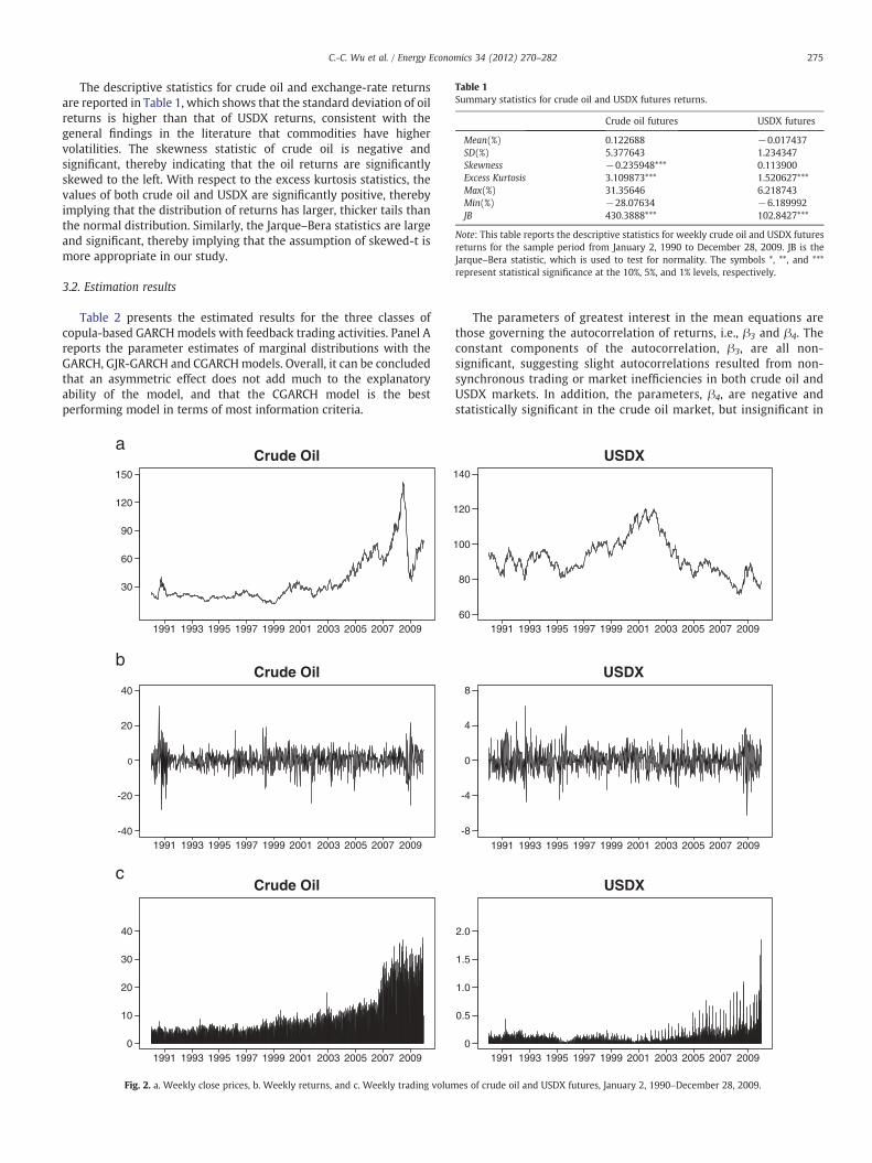
Table 1Summary statistics for crude oil and USDX futures returns.

Crude oil futures USDX futures

Mean(%) 0.122688 −0.017437SD(%) 5.377643 1.234347Skewness −0.235948*** 0.113900Excess Kurtosis 3.109873*** 1.520627***Max(%) 31.35646 6.218743Min(%) −28.07634 −6.189992JB 430.3888*** 102.8427***

Note: This table reports the descriptive statistics for weekly crude oil and USDX futuresreturns for the sample period from January 2, 1990 to December 28, 2009. JB is theJarque–Bera statistic, which is used to test for normality. The symbols *, **, and ***represent statistical significance at the 10%, 5%, and 1% levels, respectively.


The descriptive statistics for crude oil and exchange-rate returnsare reported in Table 1, which shows that the standard deviation of oilreturns is higher than that of USDX returns, consistent with thegeneral findings in the literature that commodities have highervolatilities. The skewness statistic of crude oil is negative andsignificant, thereby indicating that the oil returns are significantlyskewed to the left. With respect to the excess kurtosis statistics, thevalues of both crude oil and USDX are significantly positive, therebyimplying that the distribution of returns has larger, thicker tails thanthe normal distribution. Similarly, the Jarque–Bera statistics are largeand significant, thereby implying that the assumption of skewed-t ismore appropriate in our study.

3.2. Estimation results

Table 2 presents the estimated results for the three classes ofcopula-based GARCHmodels with feedback trading activities. Panel Areports the parameter estimates of marginal distributions with theGARCH, GJR-GARCH and CGARCHmodels. Overall, it can be concludedthat an asymmetric effect does not add much to the explanatoryability of the model, and that the CGARCH model is the bestperforming model in terms of most information criteria.

Crude Oil

30

60

90

120

150

Crude Oil

-40

-20

0

20

40

Crude Oil

0

10

20

30

40

1991 1993 1995 1997 1999 2001 2003 2005 2007 2009

1991 1993 1995 1997 1999 2001 2003 2005 2007 2009

1991 1993 1995 1997 1999 2001 2003 2005 2007 2009

a

b

c

Fig. 2. a. Weekly close prices, b. Weekly returns, and c. Weekly trading volum

The parameters of greatest interest in the mean equations arethose governing the autocorrelation of returns, i.e., β3 and β4. Theconstant components of the autocorrelation, β3, are all non-significant, suggesting slight autocorrelations resulted from non-synchronous trading or market inefficiencies in both crude oil andUSDX markets. In addition, the parameters, β4, are negative andstatistically significant in the crude oil market, but insignificant in

USDX

60

80

100

120

140

USDX

-8

-4

0

4

8

USDX

1991 1993 1995 1997 1999 2001 2003 2005 2007 2009

1991 1993 1995 1997 1999 2001 2003 2005 2007 2009

1991 1993 1995 1997 1999 2001 2003 2005 2007 2009

0

0.5

1.0

1.5

2.0

es of crude oil and USDX futures, January 2, 1990–December 28, 2009.

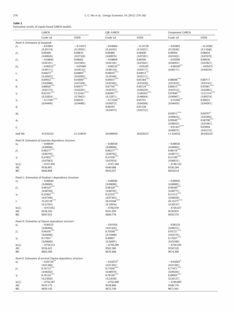
Table 2Estimation results of copula-based GARCH models.

GARCH GJR–GARCH Component GARCH

Crude oil USDX Crude oil USDX Crude oil USDX

Panel A: Estimation of marginalsβ1 −0.03861 −0.14353 −0.04460 −0.14130 −0.05865 −0.14382

(0.20174) (0.10501) (0.24193) (0.10251) (0.23638) (0.11046)β2 0.00440 0.08835 0.00480 0.08440 0.00994 0.08854

(0.00826) (0.07328) (0.00976) (0.07201) (0.01022) (0.07679)β3 −0.04842 0.08662 −0.04804 0.08306 −0.05099 0.08650

(0.05101) (0.07603) (0.05145) (0.07641) (0.04953) (0.07827)β4 −0.00223⁎⁎ −0.05489 −0.00216⁎⁎ −0.05245 −0.00249⁎⁎ −0.05473

(0.00111) (0.04122) (0.00110) (0.04117) (0.00111) (0.04229)ci 0.66673⁎⁎ 0.04805⁎⁎ 0.68935⁎⁎⁎ 0.04912⁎⁎

(0.26925) (0.02083) (0.29160) (0.02111)ai 0.09952⁎⁎⁎ 0.05809⁎⁎⁎ 0.09837⁎⁎⁎ 0.05384⁎⁎⁎ 0.08048⁎⁎⁎ 0.00717

(0.02088) (0.01456) (0.02582) (0.01650) (0.01819) (0.03161)bi 0.88026⁎⁎⁎ 0.90977⁎⁎⁎ 0.87709⁎⁎⁎ 0.90724⁎⁎⁎ 0.86015⁎⁎⁎ 0.95981⁎⁎⁎

(0.02173) (0.02201) (0.02337) (0.00229) (0.03312) (0.02861)ηi 8.92101⁎⁎⁎ 12.52421⁎⁎⁎ 9.60491⁎⁎⁎ 12.86263⁎⁎⁎ 9.97846⁎⁎⁎ 12.51314⁎⁎⁎

(0.52824) (0.70421) (0.12871) (0.48664) (0.90967) (0.89374)λi −0.17281⁎⁎⁎ 0.06025 −0.17204⁎⁎ 0.05791 −0.16366⁎⁎ 0.06022

(0.04496) (0.04485) (0.04512) (0.04506) (0.04459) (0.04501)di 0.00293 0.01238

(0.03073) (0.02722)ϖi 0.05011⁎⁎⁎ 0.04797⁎

(0.00822) (0.02492)ϕi 0.99949⁎⁎⁎ 0.96790⁎⁎⁎

(0.00033) (0.01967)ζi −0.01437⁎⁎⁎ 0.05094

(0.00073) (0.03153)Half life 33.932522 21.218035 29.690959 20.829237 11.324932 20.643225

Panel B: Estimation of Gaussian dependence structureαc −0.00039 −0.00038 −0.00036

(0.00088) (0.00088) (0.00083)βc 0.98277⁎⁎⁎ 0.98277⁎⁎⁎ 0.98310⁎⁎⁎

(0.00795) (0.00792) (0.00771)γc 0.21852⁎⁎⁎ 0.21936⁎⁎⁎ 0.21100⁎⁎⁎

(0.07063) (0.07054) (0.06631)ln(L) −4747.450 −4747.344 −4740.122AIC 9536.901 9540.688 9530.244BIC 9640.868 9654.557 9654.014

Panel C: Estimation of Student-t dependence structureαc −0.00044 −0.00046 −0.00045

(0.00089) (0.00090) (0.00085)βc 0.98325⁎⁎⁎ 0.98328⁎⁎⁎ 0.98380⁎⁎⁎

(0.00794) (0.00795) (0.00771)γc 0.22062⁎⁎⁎ 0.22225⁎⁎⁎ 0.21313⁎⁎⁎

(0.07298) (0.07365) (0.06920)υ 33.29138⁎⁎⁎ 26.55568⁎⁎⁎ 26.15277⁎⁎⁎

(0.21593) (0.19956) (0.26537)ln(L) −4747.052 −4746.979 −4739.427AIC 9538.105 9541.959 9530.855BIC 9647.023 9660.778 9659.576

Panel D: Estimation of Clayton dependence structureαc −0.00523 −0.01956 −0.00329

(0.00494) (0.01426) (0.00251)βc 0.94356⁎⁎⁎ 0.79598⁎⁎⁎ 0.95721⁎⁎⁎

(0.04286) (0.14448) (0.02155)γc 0.17951⁎ 0.49897 0.15261⁎⁎⁎

(0.09660) (0.36001) (0.05380)ln(L) −4758.212 −4758.209 −4750.265AIC 9558.423 9562.580 9550.529BIC 9662.390 9676.448 9674.300

Panel E: Estimation of survival Clayton dependence structureαc −0.02726⁎⁎ −0.02675⁎ −0.02603⁎

(0.01386) (0.01392) (0.01385)βc 0.76715⁎⁎⁎ 0.77056⁎⁎⁎ 0.77471⁎⁎⁎

(0.08202) (0.08919) (0.09283)γc 0.78126⁎⁎⁎ 0.78198⁎⁎⁎ 0.68003⁎⁎⁎

(0.23828) (0.23630) (0.26127)ln(L) −4756.587 −4756.440 −4749.085AIC 9555.175 9558.880 9548.170BIC 9659.142 9672.749 9671.941


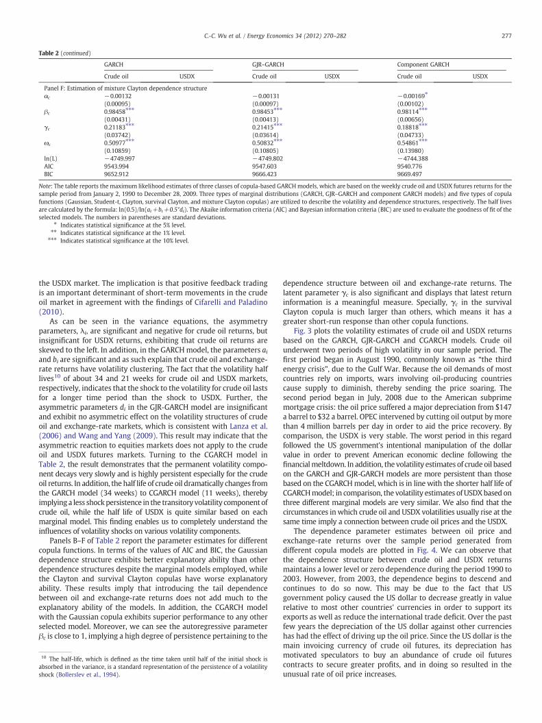
Table 2 (continued)

GARCH GJR–GARCH Component GARCH

Crude oil USDX Crude oil USDX Crude oil USDX

Panel F: Estimation of mixture Clayton dependence structureαc −0.00132 −0.00131 −0.00169⁎

(0.00095) (0.00097) (0.00102)βc 0.98458⁎⁎⁎ 0.98453⁎⁎⁎ 0.98114⁎⁎⁎

(0.00431) (0.00413) (0.00656)γc 0.21183⁎⁎⁎ 0.21415⁎⁎⁎ 0.18818⁎⁎⁎

(0.03742) (0.03614) (0.04733)ωc 0.50977⁎⁎⁎ 0.50832⁎⁎⁎ 0.54861⁎⁎⁎

(0.10859) (0.10805) (0.13980)ln(L) −4749.997 −4749.802 −4744.388AIC 9543.994 9547.603 9540.776BIC 9652.912 9666.423 9669.497

Note: The table reports the maximum likelihood estimates of three classes of copula-based GARCHmodels, which are based on the weekly crude oil and USDX futures returns for thesample period from January 2, 1990 to December 28, 2009. Three types of marginal distributions (GARCH, GJR–GARCH and component GARCH models) and five types of copulafunctions (Gaussian, Student-t, Clayton, survival Clayton, and mixture Clayton copulas) are utilized to describe the volatility and dependence structures, respectively. The half livesare calculated by the formula: ln(0.5)/ln(ai+bi+0.5*di). The Akaike information criteria (AIC) and Bayesian information criteria (BIC) are used to evaluate the goodness of fit of theselected models. The numbers in parentheses are standard deviations.

⁎ Indicates statistical significance at the 5% level.⁎⁎ Indicates statistical significance at the 1% level.⁎⁎⁎ Indicates statistical significance at the 10% level.


the USDX market. The implication is that positive feedback tradingis an important determinant of short-term movements in the crudeoil market in agreement with the findings of Cifarelli and Paladino(2010).

As can be seen in the variance equations, the asymmetryparameters, λi, are significant and negative for crude oil returns, butinsignificant for USDX returns, exhibiting that crude oil returns areskewed to the left. In addition, in the GARCHmodel, the parameters aiand bi are significant and as such explain that crude oil and exchange-rate returns have volatility clustering. The fact that the volatility halflives10 of about 34 and 21 weeks for crude oil and USDX markets,respectively, indicates that the shock to the volatility for crude oil lastsfor a longer time period than the shock to USDX. Further, theasymmetric parameters di in the GJR-GARCH model are insignificantand exhibit no asymmetric effect on the volatility structures of crudeoil and exchange-rate markets, which is consistent with Lanza et al.(2006) and Wang and Yang (2009). This result may indicate that theasymmetric reaction to equities markets does not apply to the crudeoil and USDX futures markets. Turning to the CGARCH model inTable 2, the result demonstrates that the permanent volatility compo-nent decays very slowly and is highly persistent especially for the crudeoil returns. In addition, the half life of crude oil dramatically changes fromthe GARCH model (34 weeks) to CGARCH model (11 weeks), therebyimplying a less shockpersistence in the transitory volatility component ofcrude oil, while the half life of USDX is quite similar based on eachmarginal model. This finding enables us to completely understand theinfluences of volatility shocks on various volatility components.

Panels B–F of Table 2 report the parameter estimates for differentcopula functions. In terms of the values of AIC and BIC, the Gaussiandependence structure exhibits better explanatory ability than otherdependence structures despite the marginal models employed, whilethe Clayton and survival Clayton copulas have worse explanatoryability. These results imply that introducing the tail dependencebetween oil and exchange-rate returns does not add much to theexplanatory ability of the models. In addition, the CGARCH modelwith the Gaussian copula exhibits superior performance to any otherselected model. Moreover, we can see the autoregressive parameterβc is close to 1, implying a high degree of persistence pertaining to the

10 The half-life, which is defined as the time taken until half of the initial shock isabsorbed in the variance, is a standard representation of the persistence of a volatilityshock (Bollerslev et al., 1994).

dependence structure between oil and exchange-rate returns. Thelatent parameter γc is also significant and displays that latest returninformation is a meaningful measure. Specially, γc in the survivalClayton copula is much larger than others, which means it has agreater short-run response than other copula functions.

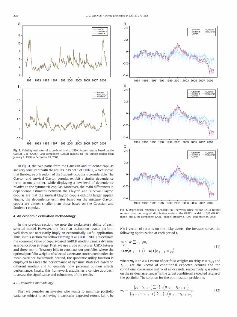
Fig. 3 plots the volatility estimates of crude oil and USDX returnsbased on the GARCH, GJR-GARCH and CGARCH models. Crude oilunderwent two periods of high volatility in our sample period. Thefirst period began in August 1990, commonly known as “the thirdenergy crisis”, due to the Gulf War. Because the oil demands of mostcountries rely on imports, wars involving oil-producing countriescause supply to diminish, thereby sending the price soaring. Thesecond period began in July, 2008 due to the American subprimemortgage crisis: the oil price suffered a major depreciation from $147a barrel to $32 a barrel. OPEC intervened by cutting oil output by morethan 4 million barrels per day in order to aid the price recovery. Bycomparison, the USDX is very stable. The worst period in this regardfollowed the US government's intentional manipulation of the dollarvalue in order to prevent American economic decline following thefinancialmeltdown. In addition, the volatility estimates of crude oil basedon the GARCH and GJR-GARCH models are more persistent than thosebased on the CGARCHmodel, which is in line with the shorter half life ofCGARCHmodel; in comparison, the volatility estimates of USDXbased onthree different marginal models are very similar. We also find that thecircumstances in which crude oil and USDX volatilities usually rise at thesame time imply a connection between crude oil prices and the USDX.

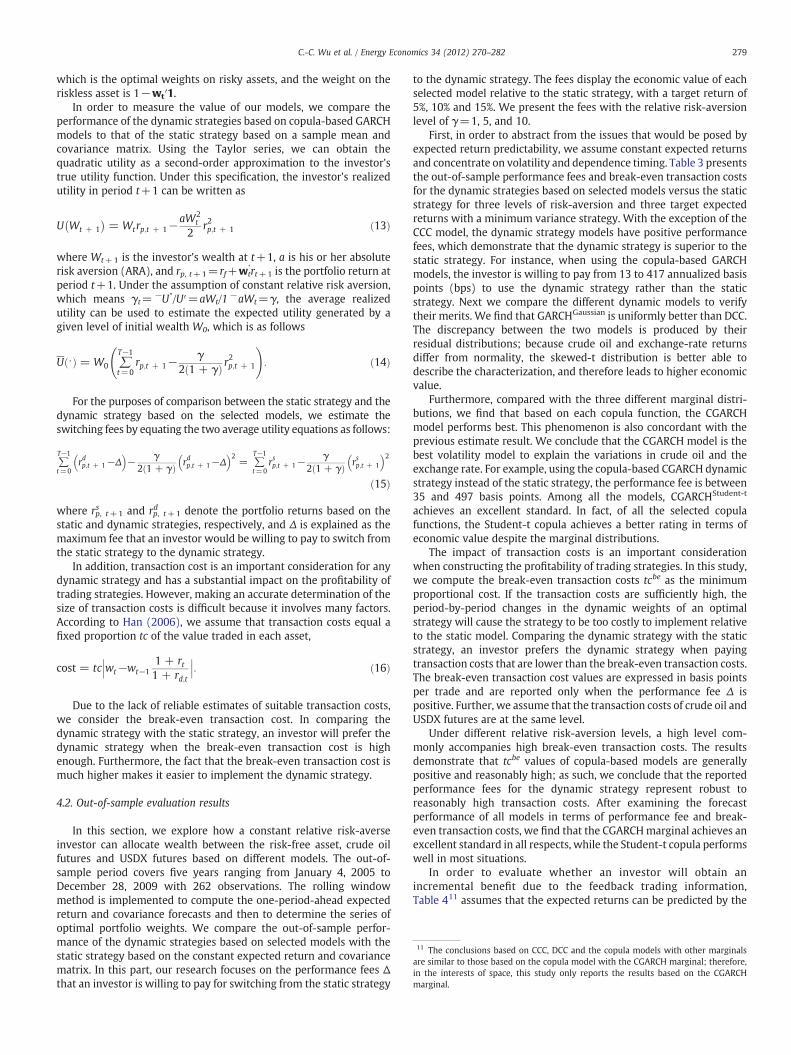
The dependence parameter estimates between oil price andexchange-rate returns over the sample period generated fromdifferent copula models are plotted in Fig. 4. We can observe thatthe dependence structure between crude oil and USDX returnsmaintains a lower level or zero dependence during the period 1990 to2003. However, from 2003, the dependence begins to descend andcontinues to do so now. This may be due to the fact that USgovernment policy caused the US dollar to decrease greatly in valuerelative to most other countries' currencies in order to support itsexports as well as reduce the international trade deficit. Over the pastfew years the depreciation of the US dollar against other currencieshas had the effect of driving up the oil price. Since the US dollar is themain invoicing currency of crude oil futures, its depreciation hasmotivated speculators to buy an abundance of crude oil futurescontracts to secure greater profits, and in doing so resulted in theunusual rate of oil price increases.

2

4

6

8

10

12

GARCHGJRGARCHCGARCH

0.5

1

1.5

2

2.5

GARCHGJRGARCHCGARCH

1991

b

a

1993 1995 1997 1999 2001 2003 2005 2007 2009

1991 1993 1995 1997 1999 2001 2003 2005 2007 2009

Fig. 3. Volatility estimates of a. crude oil and b. USDX futures returns based on theGARCH, GJR -GARCH, and component GARCH models for the sample period fromJanuary 2, 1990 to December 28, 2009.

1991 1993 1995 1997 1999 2001 2003 2005 2007 2009

1991 1993 1995 1997 1999 2001 2003 2005 2007 2009

1991 1993 1995 1997 1999 2001 2003 2005 2007 2009

-0.4

-0.2

0

0.2

0.4

-0.4

-0.2

0

0.2

0.4

-0.4

-0.2

0

0.2

0.4GaussianStudent-tClayton

SClaytonMixClayton

a

b

c

GaussianStudent-tClayton

SClaytonMixClayton

GaussianStudent-tClayton

SClaytonMixClayton

Fig. 4. Dependence estimates (Kendall's tau) between crude oil and USDX futuresreturns based on marginal distribution under a. the GARCH model, b. GJR -GARCHmodel, and c. the component GARCH model, January 2, 1990 -December 28, 2009.


In Fig. 4, the two paths from the Gaussian and Student-t copulasare very consistent with the results in Panel C of Table 2, which showsthat the degree of freedomof the Student-t copula is considerable. TheClayton and survival Clayton copulas exhibit a similar dependencetrend to one another, while displaying a low level of dependencerelative to the symmetric copulas. Moreover, the main differences independence estimates between the Clayton and survival Claytoncopulas are that the survival Clayton copula exhibits larger ripples.Finally, the dependence estimates based on the mixture Claytoncopula are almost smaller than those based on the Gaussian andStudent-t copulas.

4. An economic evaluation methodology

In the previous section, we note the explanatory ability of eachselected model. However, the fact that estimation results performwell does not necessarily imply an economically useful application.Thus, in this section, we follow Fleming et al. (2001, 2003) to evaluatethe economic value of copula-based GARCH models using a dynamicasset-allocation strategy. First, we use crude oil futures, USDX futuresand three-month Treasury bills to construct our portfolio, where theoptimal portfolio weights of selected assets are constructed under themean–variance framework. Second, the quadratic utility function isemployed to assess the performance of dynamic strategies based ondifferent models and to quantify how personal opinion affectsperformance. Finally, this framework establishes a concise approachto assess the significance and robustness of the results.

4.1. Evaluation methodology

First we consider an investor who wants to minimize portfoliovariance subject to achieving a particular expected return. Let rt be

N×1 vector of returns on the risky assets; the investor solves thefollowing optimization at each period t,

minwt

w′t∑t + 1wt

s:t:w′tμt + 1 + 1−w′

t1� �

rf ;t + 1 = μ⁎pð11Þ

wherewt is an N×1 vector of portfolio weights on risky assets, μt andΣt+ 1 are the vector of conditional expected returns and theconditional covariance matrix of risky assets, respectively, rf is returnon the riskless asset and μp⁎ is the target conditional expected return ofthe portfolio. The solution for the optimization problem is

wt =μ�p−rf ;t + 1

� �∑−1

t + 1 μt + 1−rf ;t + 11� �

μt + 1−rf ;t + 11� �

′∑−1t + 1 μt + 1−rf ;t + 11

� � ; ð12Þ

11 The conclusions based on CCC, DCC and the copula models with other marginalsare similar to those based on the copula model with the CGARCH marginal; therefore,in the interests of space, this study only reports the results based on the CGARCHmarginal.


which is the optimal weights on risky assets, and the weight on theriskless asset is 1−wt′1.

In order to measure the value of our models, we compare theperformance of the dynamic strategies based on copula-based GARCHmodels to that of the static strategy based on a sample mean andcovariance matrix. Using the Taylor series, we can obtain thequadratic utility as a second-order approximation to the investor'strue utility function. Under this specification, the investor's realizedutility in period t+1 can be written as

U Wt + 1� �

= Wtrp;t + 1−aW2

t

2r2p;t + 1 ð13Þ

where Wt+1 is the investor's wealth at t+1, a is his or her absoluterisk aversion (ARA), and rp, t+1=rf+wt

'rt+1 is the portfolio return atperiod t+1. Under the assumption of constant relative risk aversion,which means γt=−U″/U′=aWt/1

−aWt=γ, the average realizedutility can be used to estimate the expected utility generated by agiven level of initial wealth W0, which is as follows

U ⋅ð Þ = W0 ∑T−1

t=0rp;t + 1−

γ2 1 + γð Þ r

2p;t + 1

!: ð14Þ

For the purposes of comparison between the static strategy and thedynamic strategy based on the selected models, we estimate theswitching fees by equating the two average utility equations as follows:

∑T−1

t=0rdp;t + 1−Δ� �

− γ2 1 + γð Þ rdp;t + 1−Δ

� �2= ∑

T−1

t=0rsp;t + 1−

γ2 1 + γð Þ rsp;t + 1

� �2ð15Þ

where rp, t+1s and rp, t+1

d denote the portfolio returns based on thestatic and dynamic strategies, respectively, and Δ is explained as themaximum fee that an investor would be willing to pay to switch fromthe static strategy to the dynamic strategy.

In addition, transaction cost is an important consideration for anydynamic strategy and has a substantial impact on the profitability oftrading strategies. However, making an accurate determination of thesize of transaction costs is difficult because it involves many factors.According to Han (2006), we assume that transaction costs equal afixed proportion tc of the value traded in each asset,

cost = tcwt−wt−1

1 + rt1 + rd;t

: ð16Þ

Due to the lack of reliable estimates of suitable transaction costs,we consider the break-even transaction cost. In comparing thedynamic strategy with the static strategy, an investor will prefer thedynamic strategy when the break-even transaction cost is highenough. Furthermore, the fact that the break-even transaction cost ismuch higher makes it easier to implement the dynamic strategy.

4.2. Out-of-sample evaluation results

In this section, we explore how a constant relative risk-averseinvestor can allocate wealth between the risk-free asset, crude oilfutures and USDX futures based on different models. The out-of-sample period covers five years ranging from January 4, 2005 toDecember 28, 2009 with 262 observations. The rolling windowmethod is implemented to compute the one-period-ahead expectedreturn and covariance forecasts and then to determine the series ofoptimal portfolio weights. We compare the out-of-sample perfor-mance of the dynamic strategies based on selected models with thestatic strategy based on the constant expected return and covariancematrix. In this part, our research focuses on the performance fees Δthat an investor is willing to pay for switching from the static strategy

to the dynamic strategy. The fees display the economic value of eachselected model relative to the static strategy, with a target return of5%, 10% and 15%. We present the fees with the relative risk-aversionlevel of γ=1, 5, and 10.

First, in order to abstract from the issues that would be posed byexpected return predictability, we assume constant expected returnsand concentrate on volatility and dependence timing. Table 3 presentsthe out-of-sample performance fees and break-even transaction costsfor the dynamic strategies based on selected models versus the staticstrategy for three levels of risk-aversion and three target expectedreturns with a minimum variance strategy. With the exception of theCCC model, the dynamic strategy models have positive performancefees, which demonstrate that the dynamic strategy is superior to thestatic strategy. For instance, when using the copula-based GARCHmodels, the investor is willing to pay from 13 to 417 annualized basispoints (bps) to use the dynamic strategy rather than the staticstrategy. Next we compare the different dynamic models to verifytheir merits. We find that GARCHGaussian is uniformly better than DCC.The discrepancy between the two models is produced by theirresidual distributions; because crude oil and exchange-rate returnsdiffer from normality, the skewed-t distribution is better able todescribe the characterization, and therefore leads to higher economicvalue.

Furthermore, compared with the three different marginal distri-butions, we find that based on each copula function, the CGARCHmodel performs best. This phenomenon is also concordant with theprevious estimate result. We conclude that the CGARCH model is thebest volatility model to explain the variations in crude oil and theexchange rate. For example, using the copula-based CGARCH dynamicstrategy instead of the static strategy, the performance fee is between35 and 497 basis points. Among all the models, CGARCHStudent-t

achieves an excellent standard. In fact, of all the selected copulafunctions, the Student-t copula achieves a better rating in terms ofeconomic value despite the marginal distributions.

The impact of transaction costs is an important considerationwhen constructing the profitability of trading strategies. In this study,we compute the break-even transaction costs tcbe as the minimumproportional cost. If the transaction costs are sufficiently high, theperiod-by-period changes in the dynamic weights of an optimalstrategy will cause the strategy to be too costly to implement relativeto the static model. Comparing the dynamic strategy with the staticstrategy, an investor prefers the dynamic strategy when payingtransaction costs that are lower than the break-even transaction costs.The break-even transaction cost values are expressed in basis pointsper trade and are reported only when the performance fee Δ ispositive. Further, we assume that the transaction costs of crude oil andUSDX futures are at the same level.

Under different relative risk-aversion levels, a high level com-monly accompanies high break-even transaction costs. The resultsdemonstrate that tcbe values of copula-based models are generallypositive and reasonably high; as such, we conclude that the reportedperformance fees for the dynamic strategy represent robust toreasonably high transaction costs. After examining the forecastperformance of all models in terms of performance fee and break-even transaction costs, we find that the CGARCHmarginal achieves anexcellent standard in all respects, while the Student-t copula performswell in most situations.

In order to evaluate whether an investor will obtain anincremental benefit due to the feedback trading information,Table 411 assumes that the expected returns can be predicted by the

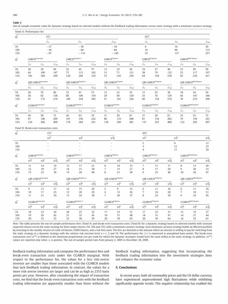
Table 3Out-of-sample economic value for dynamic strategy based on selected models without the feedback trading information versus static strategy with a minimum variance strategy.

Panel A: Performance fee

μp⁎ CCC DCC

△1 △5 △10 △1 △5 △10

5% −27 −30 −34 6 16 3010% −56 −68 −84 16 60 11515% −87 −114 −149 33 131 257

μp⁎ GARCHGaussian GARCHStudent-t GARCHClayton GARCHSClayton GARCHMixClayton

△1 △5 △10 △1 △5 △10 △1 △5 △10 △1 △5 △10 △1 △5 △10

5% 30 39 50 35 45 57 13 23 36 16 27 40 23 39 5910% 64 100 147 75 113 162 31 71 121 38 79 132 53 117 19715% 102 184 290 120 206 316 53 143 259 64 158 278 92 234 417

μp⁎ GJR-GARCHGaussian GJR-GARCHStudent-t GJR-GARCHClayton GJR-GARCHSClayton GJR-GARCHMixClayton

△1 △5 △10 △1 △5 △10 △1 △5 △10 △1 △5 △10 △1 △5 △10

5% 26 35 46 32 41 53 12 22 35 15 25 38 18 34 5410% 56 92 138 68 106 154 29 69 120 35 76 129 45 107 18615% 91 172 276 109 194 303 51 141 256 60 154 274 78 219 399

μp⁎ CGARCHGaussian CGARCHStudent-t CGARCHClayton CGARCHSClayton CGARCHMixClayton

△1 △5 △10 △1 △5 △10 △1 △5 △10 △1 △5 △10 △1 △5 △10

5% 45 58 73 50 63 79 37 50 67 37 50 67 35 53 7510% 97 146 209 107 158 222 80 133 200 81 134 202 79 150 24115% 154 266 409 170 284 431 130 249 401 131 252 406 132 292 497

Panel B: Break-even transaction costs

μp⁎ CCC DCC

tc1be tc5

be tc10be tc1

be tc5be tc10

be

5% – – – 2 6 1210% – – – 3 12 2315% – – – 4 17 34

μp⁎ GARCHGaussian GARCHStudent-t GARCHClayton GARCHSClayton GARCHMixClayton

tc1be tc5

be tc10be tc1

be tc5be tc10

be tc1be tc5

be tc10be tc1

be tc5be tc10

be tc1be tc5

be tc10be

5% 11 14 19 13 17 21 6 10 15 7 11 17 8 13 2010% 12 18 27 14 21 30 7 15 27 8 17 29 9 20 3315% 13 23 36 15 26 40 8 21 38 9 23 40 10 26 47

μp⁎ GJR-GARCHGaussian GJR-GARCHStudent-t GJR-GARCHClayton GJR-GARCHSClayton GJR-GARCHMixClayton

tc1be tc5

be tc10be tc1

be tc5be tc10

be tc1be tc5

be tc10be tc1

be tc5be tc10

be tc1be tc5

be tc10be

5% 9 13 17 12 15 20 5 9 15 6 11 16 6 11 1810% 10 17 25 13 20 29 6 15 26 7 16 28 7 18 3115% 11 21 34 13 24 38 7 20 37 8 22 39 9 24 45


tc1be tc5

be tc10be tc1

be tc5be tc10

be tc1be tc5

be tc10be tc1

be tc5be tc10

be tc1be tc5

be tc10be

5% 18 23 29 20 25 32 17 23 31 17 23 31 13 19 2710% 19 29 42 21 32 45 19 31 48 18 31 47 14 27 4415% 20 35 55 23 38 59 20 39 65 20 39 64 16 35 61

Note: The table presents the out-of-sample performance fees (Panel A) and break-even transaction costs (Panel B) for a dynamic strategy based on selected models with constantexpected returns versus the static strategy for three target returns (5%, 10% and 15%)with aminimum variance strategy. Eachminimum variance strategy builds an efficient portfolioby investing in the weekly returns of crude oil futures, USDX futures, and a risk-free asset. The fees are denoted as the amount which an investor is willing to pay for switching fromthe static strategy to a dynamic strategy with the relative risk aversion level γ=1, 5 and 10. The performance fee (△) is expressed in annualized basis points. The break-eventransaction cost (tcbe) is defined as the minimum proportional cost per trade for which the dynamic strategies would have the same utility as the static strategy. In addition, (tcbe)values are reported only when △ is positive. The out-of-sample period runs from January 2, 2005 to December 28, 2009.


feedback trading information and computes the performance fees andbreak-even transaction costs under the CGARCH marginal. Withrespect to the performance fee, the values for a less risk-averseinvestor are smaller than those associated with the CGARCH modelsthat lack feedback trading information. In contrast, the values for amore risk-averse investor are larger and can be as high as 2353 basispoints per year. However, after considering the impact of transactioncosts, we find that the break-even transaction costs with the feedbacktrading information are apparently smaller than those without the

feedback trading information, suggesting that incorporating thefeedback trading information into the investment strategies doesnot enhance the economic value.

5. Conclusions

In recent years, both oil commodity prices and the US dollar currencyhave experienced unprecedented high fluctuations while exhibitingsignificantly opposite trends. This negative relationship has enabled the

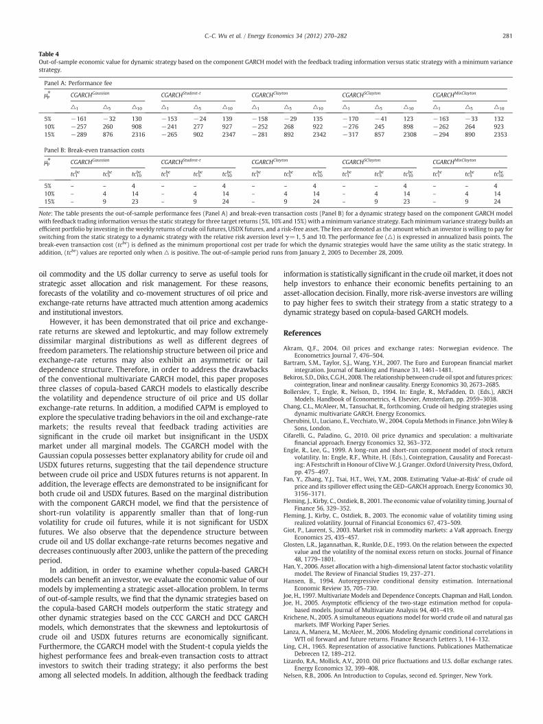
Table 4Out-of-sample economic value for dynamic strategy based on the component GARCH model with the feedback trading information versus static strategy with a minimum variancestrategy.

Panel A: Performance fee


△1 △5 △10 △1 △5 △10 △1 △5 △10 △1 △5 △10 △1 △5 △10

5% −161 −32 130 −153 −24 139 −158 −29 135 −170 −41 123 −163 −33 13210% −257 260 908 −241 277 927 −252 268 922 −276 245 898 −262 264 92315% −289 876 2316 −265 902 2347 −281 892 2342 −317 857 2308 −294 890 2353

Panel B: Break-even transaction costs


tc1be tc5

be tc10be tc1

be tc5be tc10

be tc1be tc5

be tc10be tc1

be tc5be tc10

be tc1be tc5

be tc10be

5% – – 4 – – 4 – – 4 – – 4 – – 410% – 4 14 – 4 14 – 4 14 – 4 14 – 4 1415% – 9 23 – 9 24 – 9 24 – 9 23 – 9 24

Note: The table presents the out-of-sample performance fees (Panel A) and break-even transaction costs (Panel B) for a dynamic strategy based on the component GARCH modelwith feedback trading information versus the static strategy for three target returns (5%, 10% and 15%) with aminimum variance strategy. Eachminimum variance strategy builds anefficient portfolio by investing in theweekly returns of crude oil futures, USDX futures, and a risk-free asset. The fees are denoted as the amount which an investor is willing to pay forswitching from the static strategy to a dynamic strategy with the relative risk aversion level γ=1, 5 and 10. The performance fee (△) is expressed in annualized basis points. Thebreak-even transaction cost (tcbe) is defined as the minimum proportional cost per trade for which the dynamic strategies would have the same utility as the static strategy. Inaddition, (tcbe) values are reported only when △ is positive. The out-of-sample period runs from January 2, 2005 to December 28, 2009.


oil commodity and the US dollar currency to serve as useful tools forstrategic asset allocation and risk management. For these reasons,forecasts of the volatility and co-movement structures of oil price andexchange-rate returns have attracted much attention among academicsand institutional investors.

However, it has been demonstrated that oil price and exchange-rate returns are skewed and leptokurtic, and may follow extremelydissimilar marginal distributions as well as different degrees offreedom parameters. The relationship structure between oil price andexchange-rate returns may also exhibit an asymmetric or taildependence structure. Therefore, in order to address the drawbacksof the conventional multivariate GARCH model, this paper proposesthree classes of copula-based GARCH models to elastically describethe volatility and dependence structure of oil price and US dollarexchange-rate returns. In addition, a modified CAPM is employed toexplore the speculative trading behaviors in the oil and exchange-ratemarkets; the results reveal that feedback trading activities aresignificant in the crude oil market but insignificant in the USDXmarket under all marginal models. The CGARCH model with theGaussian copula possesses better explanatory ability for crude oil andUSDX futures returns, suggesting that the tail dependence structurebetween crude oil price and USDX futures returns is not apparent. Inaddition, the leverage effects are demonstrated to be insignificant forboth crude oil and USDX futures. Based on the marginal distributionwith the component GARCH model, we find that the persistence ofshort-run volatility is apparently smaller than that of long-runvolatility for crude oil futures, while it is not significant for USDXfutures. We also observe that the dependence structure betweencrude oil and US dollar exchange-rate returns becomes negative anddecreases continuously after 2003, unlike the pattern of the precedingperiod.

In addition, in order to examine whether copula-based GARCHmodels can benefit an investor, we evaluate the economic value of ourmodels by implementing a strategic asset-allocation problem. In termsof out-of-sample results, we find that the dynamic strategies based onthe copula-based GARCH models outperform the static strategy andother dynamic strategies based on the CCC GARCH and DCC GARCHmodels, which demonstrates that the skewness and leptokurtosis ofcrude oil and USDX futures returns are economically significant.Furthermore, the CGARCH model with the Student-t copula yields thehighest performance fees and break-even transaction costs to attractinvestors to switch their trading strategy; it also performs the bestamong all selected models. In addition, although the feedback trading

information is statistically significant in the crude oil market, it does nothelp investors to enhance their economic benefits pertaining to anasset-allocation decision. Finally, more risk-averse investors are willingto pay higher fees to switch their strategy from a static strategy to adynamic strategy based on copula-based GARCH models.

References

Akram, Q.F., 2004. Oil prices and exchange rates: Norwegian evidence. TheEconometrics Journal 7, 476–504.

Bartram, S.M., Taylor, S.J., Wang, Y.H., 2007. The Euro and European financial marketintegration. Journal of Banking and Finance 31, 1461–1481.

Bekiros, S.D., Diks, C.G.H., 2008. The relationship between crude oil spot and futures prices:cointegration, linear and nonlinear causality. Energy Economics 30, 2673–2685.

Bollerslev, T., Engle, R., Nelson, D., 1994. In: Engle, R., McFadden, D. (Eds.), ARCHModels. Handbook of Econometrics, 4. Elsevier, Amsterdam, pp. 2959–3038.

Chang, C.L., McAleer, M., Tansuchat, R., forthcoming. Crude oil hedging strategies usingdynamic multivariate GARCH. Energy Economics.

Cherubini, U., Luciano, E., Vecchiato, W., 2004. Copula Methods in Finance. JohnWiley &Sons, London.

Cifarelli, G., Paladino, G., 2010. Oil price dynamics and speculation: a multivariatefinancial approach. Energy Economics 32, 363–372.

Engle, R., Lee, G., 1999. A long-run and short-run component model of stock returnvolatility. In: Engle, R.F., White, H. (Eds.), Cointegration, Causality and Forecast-ing: A Festschrift in Honour of CliveW. J. Granger. Oxford University Press, Oxford,pp. 475–497.

Fan, Y., Zhang, Y.J., Tsai, H.T., Wei, Y.M., 2008. Estimating ‘Value-at-Risk’ of crude oilprice and its spillover effect using the GED–GARCH approach. Energy Economics 30,3156–3171.

Fleming, J., Kirby, C., Ostdiek, B., 2001. The economic value of volatility timing. Journal ofFinance 56, 329–352.

Fleming, J., Kirby, C., Ostdiek, B., 2003. The economic value of volatility timing usingrealized volatility. Journal of Financial Economics 67, 473–509.

Giot, P., Laurent, S., 2003. Market risk in commodity markets: a VaR approach. EnergyEconomics 25, 435–457.

Glosten, L.R., Jagannathan, R., Runkle, D.E., 1993. On the relation between the expectedvalue and the volatility of the nominal excess return on stocks. Journal of Finance48, 1779–1801.

Han, Y., 2006. Asset allocationwith a high-dimensional latent factor stochastic volatilitymodel. The Review of Financial Studies 19, 237–271.

Hansen, B., 1994. Autoregressive conditional density estimation. InternationalEconomic Review 35, 705–730.

Joe, H., 1997. Multivariate Models and Dependence Concepts. Chapman and Hall, London.Joe, H., 2005. Asymptotic efficiency of the two-stage estimation method for copula-

based models. Journal of Multivariate Analysis 94, 401–419.Krichene, N., 2005. A simultaneous equations model for world crude oil and natural gas

markets. IMF Working Paper Series.Lanza, A., Manera, M., McAleer, M., 2006. Modeling dynamic conditional correlations in

WTI oil forward and future returns. Finance Research Letters 3, 114–132.Ling, C.H., 1965. Representation of associative functions. Publicationes Mathematicae

Debrecen 12, 189–212.Lizardo, R.A., Mollick, A.V., 2010. Oil price fluctuations and U.S. dollar exchange rates.

Energy Economics 32, 399–408.Nelsen, R.B., 2006. An Introduction to Copulas, second ed. Springer, New York.


Patton, A.L., 2006. Modelling asymmetric exchange rate dependence. InternationalEconomic Review 47, 527–556.

Sari, R., Hammoudeh, S., Soytas, U., 2009. Dynamics of oil price, precious metal prices,and exchange rate. Energy Economics 32, 351–362.

Schweizer, B., Sklar, A., 1961. Associative functions and statistical triangle inequalities.Publicationes Mathematicae Debrecen 8, 169–186.

Sentana, E., Wadhwani, S., 1992. Feedback traders and stock return autocorrelations:evidence from a century of daily data. The Economic Journal 102, 415–425.

Wang, J., Yang, M., 2009. Asymmetric volatility in foreign exchange markets. Journal ofInternational Financial Markets Institutions and Money 19, 597–615.

Yousefi, A., Wirjanto, T.S., 2004. The empirical role of the exchange rate on the crude-oilprice formation. Energy Economics 26, 783–799.

the economic value of co-movement between oil price and exchange rate using copula-based garch...

Documents