the

eart

h o

bse

rver

National Aeronautics and Space Administration

The Earth Observer. July - August 2017. Volume 29, Issue 4.

As it has done for nearly sixty years, NASA continues to push technology to enable new science. In 2014 NASA’s Science Mission Directorate’s (SMD) Advanced Technology Initiatives Program (ATIP) and the Earth Science Technology Office’s (ESTO) In-Space Validation of Earth Science Technologies (InVEST) program selected the IceCube project, a fast-track spaceflight demonstration of an 883-GHz cloud radiometer on a 3U CubeSat.1 The primary objective of IceCube is to raise the technology readiness level of the 883-GHz IceCube Cloud–Ice Radiometer (ICIR) for future Earth science missions2 by flying a commercial receiver in spaceflight demonstration. This is a high-risk “pathfinder” mission designed and built using commercial off-the-shelf com-ponents, but with the potential for great reward in testing a new measurement concept.

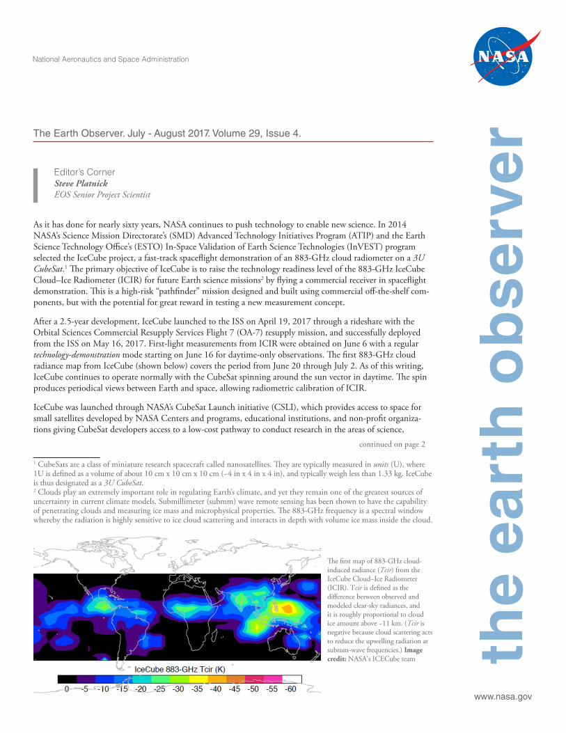
After a 2.5-year development, IceCube launched to the ISS on April 19, 2017 through a rideshare with the Orbital Sciences Commercial Resupply Services Flight 7 (OA-7) resupply mission, and successfully deployed from the ISS on May 16, 2017. First-light measurements from ICIR were obtained on June 6 with a regular technology-demonstration mode starting on June 16 for daytime-only observations. The first 883-GHz cloud radiance map from IceCube (shown below) covers the period from June 20 through July 2. As of this writing, IceCube continues to operate normally with the CubeSat spinning around the sun vector in daytime. The spin produces periodical views between Earth and space, allowing radiometric calibration of ICIR.

IceCube was launched through NASA’s CubeSat Launch initiative (CSLI), which provides access to space for small satellites developed by NASA Centers and programs, educational institutions, and non-profit organiza-tions giving CubeSat developers access to a low-cost pathway to conduct research in the areas of science,

continued on page 2

1 CubeSats are a class of miniature research spacecraft called nanosatellites. They are typically measured in units (U), where 1U is defined as a volume of about 10 cm x 10 cm x 10 cm (~4 in x 4 in x 4 in), and typically weigh less than 1.33 kg. IceCube is thus designated as a 3U CubeSat.  2 Clouds play an extremely important role in regulating Earth’s climate, and yet they remain one of the greatest sources of uncertainty in current climate models. Submillimeter (submm) wave remote sensing has been shown to have the capability of penetrating clouds and measuring ice mass and microphysical properties. The 883-GHz frequency is a spectral window whereby the radiation is highly sensitive to ice cloud scattering and interacts in depth with volume ice mass inside the cloud.

Editor’s CornerSteve PlatnickEOS Senior Project Scientist

The first map of 883-GHz cloud-induced radiance (Tcir) from the IceCube Cloud–Ice Radiometer (ICIR). Tcir is defined as the difference between observed and modeled clear-sky radiances, and it is roughly proportional to cloud ice amount above ~11 km. (Tcir is negative because cloud scattering acts to reduce the upwelling radiation at submm-wave frequencies.) Image credit: NASA's ICECube team

www.nasa.gov

The Earth Observer July - August 2017 Volume 29, Issue 402ed

itor's

cor

ner

exploration, technology development, education, or opera-tions. The initiative is an integrated cross-agency collab-orative effort led by NASA’s Human Exploration and Operations Mission Directorate to streamline and prioritize ride share and deployment opportunities of CubeSats. 

To date, NASA has selected 152 CubeSat missions from 85 unique organizations representing 38 states and the District of Columbia. In addition to IceCube, several other current or planned CubeSat missions are test-ing technology and/or studying subjects that may have applications for Earth Science. In November 2016, for example, the Radiometer Assessment using Vertically Aligned Nanotubes (RAVAN) CubeSat was launched from Vandenberg Air Force Base, collecting “first light” on January 25 of this year. RAVAN, a project led by the Johns Hopkins Applied Physics Laboratory mea-sures outgoing radiative energy. Several other CubeSats are planned for launch over the coming year. The Microwave Radiometer Technology Acceleration mis-sion (MiRaTA) will be carried into space onboard NOAA’s Joint Polar Satellite System-1 (JPSS-1) sat-ellite (scheduled to launch later this year) to collect data on temperature, water vapor, and cloud ice. The Hyper-Angular Rainbow Polarimeter (HARP), sched-uled to launch to the ISS in January 2018, will retrieve aerosol and cloud particle properties using multiangle polarimetric measurements. Two larger 6U CubeSats will launch to the ISS in March 2018: RainCube, which will measure precipitation, will be the first

active-remote-sensing radar on on CubeSat platform (Ka-band); and CubeRRT will demonstrate wideband radio frequency interference (RFI) mitigating backend technologies vital for future space-borne microwave radiometers. Similar to IceCube, these CubeSat mis-sions are all part of the InVEST program.

In addition, the Temporal Experiment for Storms and Tropical Systems Technology Demonstration (TEMPEST-D) is another 6U CubeSat that will launch in March 2018, as part of the Earth Venture Technology initiative.

The Total Solar Irradiance Sensor-1 (TSIS-1) mission passed its pre-shipment review (PSR) on July 20, 2017. Its two instruments—the Total Irradiance Monitor (TIM) and the Spectral Irradiance Monitor (SIM)—are now at KSC. The launch date remains NET November 1 on SpaceX Commercial Resupply Service-13. The TSIS-1 mission will provide absolute measurements of the total solar irradiance (TSI) and spectral solar irradi-ance (SSI), important for accurate scientific models of climate change and solar variability. TSIS-1 will con-tinue the 35-year data record of TSI measurements that is currently being maintained by the TIM instrument on the aging Solar Radiation and Climate Experiment (SORCE) spacecraft (launched in 2003) and aug-mented (since 2013) by the Total Solar Irradiance Calibration Transfer Experiment (TCTE) instrument, a joint mission with NOAA and the U.S. Air Force. 

In This Issue

Editor’s Corner Front Cover NASA Aids Study of Lake Michigan High-Ozone Events 39

Feature Articles NASA Data Suggest Future May Be The Third A-Train Symposium: Rainier Than Expected 40Summary and Perspectives on a Decade of

Constellation-Based Earth Observations 4 Announcements

Up and ATom! 2016 Atmospheric Meeting Summaries Tomography Mission Dataset Released 23

2017 ASTER Science Team Meeting Summary 19 DSCOVR EPIC and NISTAR Level-1 2017 ECOSTRESS Science Team Data Released 27

Meeting Summary 24 Coming This Fall: Publication of Summary of the Third GEDI Science Landsat Legacy Book 31

Definition Team Meeting 28 Storytelling and More: NASA Science at the 2017 AGU Fall Meeting 38CERES Science Team Meeting Summary 32

Regular FeaturesIn the NewsNASA Earth Science in the News 41NASA–MIT Study Evaluates Efficiency of Oceans Science Calendars 43as Heat Sink, Atmospheric Gases Sponge 37

Reminder: To view newsletter images in color, visit eospso.nasa.gov/earth-observer-archive.

The Earth Observer July - August 2017 Volume 29, Issue 4 03

edito

r's c

orne

rThe ECOsystem Spaceborne Thermal Radiometer Experiment on Space Station (ECOSTRESS) passed its Environmental Test Readiness Review (ETRR) and Safety Phase III Review, and final integration has begun. Delivery to KSC is anticipated to take place in August 2017 where it will be held in storage until its planned April 2018 launch. ECOSTRESS will mea-sure the temperature of plants from the ISS and use that information to better understand their water needs and responses to heat and water stress. The instrument is currently being built at JPL. The third ECOSTRESS Science Team Meeting took place May 15-17, 2017, at the University of California, Davis, and was an oppor-tunity for the team to review mission science specifica-tions, milestones, and schedules, and to discuss prog-ress towards these goals. Turn to page 24 of this issue to learn more about the status of ECOSTRESS.

The Global Ecosystem Dynamics Investigation (GEDI) continues to meet its milestones as it moves towards a scheduled December 2018 launch. Engineering model hardware fabrication and key interface testing are wrapping up, flight-model fabrication is fully under-way, integration and test facilities are ready, and the Ground System and Mission Operations Center are in preparation. GEDI is a multibeam lidar that will pro-vide Earth’s first comprehensive and high-resolution dataset of ecosystem structure. Development of the GEDI laser is also progressing well; sensor performance remains solid with good margins. An earlier issue that was causing the beam to exhibit laser side-lobes has been resolved and the laser now exhibits Gaussian spa-tial beam quality.3 The third GEDI Science Definition Team (SDT) meeting took place April 4-6, 2017, in Annapolis, MD; turn to page 28 to learn more.

In other news, the Ocean Surface Topography Mission (OSTM)/Jason-2 satellite (a partnership among NASA, NOAA, CNES, and EUMETSAT) recently marked the ninth anniversary of its launch—well exceeding its planned three-to-five-year mission. During that time, OSTM/Jason-2 has precisely measured the height of 95% of the world’s ice-free ocean every 10 days. Since October 2016, it has operated in a tandem mission with its successor, Jason-3, launched in January 2016, dou-bling coverage of the global ocean and improving data resolution for both missions.

Along with Jason-3, OSTM/Jason-2 contributes to a satellite ocean altimetry data record that began with the launch of the U.S./French Ocean Topography Experiment (Topex)/Poseidon satellite in 1992. Although OSTM/Jason-2 continues to perform well, onboard systems have aged and the harsh environment

3 GEDI’s laser footprint energy follows a two-dimensional Gaussian distribution, exhibiting stronger power in the cen-ter and fading towards the edges. The nominal footprint size (22 m) indicates the diameter within which 86% of the energy is contained.

of space has begun to take a toll on key satellite com-ponents. It was therefore decided to move the older satellite out of its current shared orbit with Jason-3 in order to safeguard the orbit for Jason-3 and its planned successor, Jason-Continuity of Service (CS)/Sentinel-6,4 planned for launch in 2020. On June 20 (the ninth anniversary of launch) Jason-2’s four mission part-ner agencies agreed to lower Jason-2’s orbit by 27 km (to 1309 km) providing a repeat orbit period of just more than one year. Final orbit transfer activities were completed on July 10. This long-repeat orbit will allow OSTM/Jason-2 to collect data along a series of very closely spaced ground tracks just 8 km apart. The result will be a new, high-resolution estimate of Earth’s aver-age sea surface height. The data obtained will also help prepare for the next generation of global satellite altim-etry missions, including the NASA/CNES/CSA/UKSA Surface Water and Ocean Topography (SWOT) mis-sion, planned for launch in 2021; and Sentinel-3B, to be launched in early 2018.

Finally, the third A-Train Symposium took place April 19-21, 2017, in Pasadena, CA. The Earth Observer has been reporting regularly on the accomplish-ments of individual instruments flying on A-Train Constellation member satellites. However, the value of the Constellation is in the synergistic use of multi-instrument observations. It was clear from the many presentations that the A-Train transformed the way we study and understand the Earth’s interrelated geophysi-cal systems. An overarching theme of the symposium was the use of A-Train data to validate and improve climate models. Clouds, aerosols, and their interac-tions were the dominant symposium topics. Other topics included improvements to numerical weather forecasting, wild fire management, drought prediction, and aircraft safety. Atmospheric composition papers included science from the A-Train’s newest member, the Orbiting Carbon Observatory-2, and recent character-istics of the Antarctic ozone hole. Looking towards the future, there was a special session on new observations, with special attention to missions from Europe such as the Sentinels, ESA’s Earth Explorer, and refinements to EUMETSAT operational polar-orbiting satellites. Please turn to page 4 to read a complete summary of the third A-Train Symposium.

4 ESA’s Sentinel missions are designed to meet the operational needs of the Copernicus programme. Each Sentinel mission is based on a constellation of two satellites to fulfill revisit and coverage requirements, providing robust datasets for Copernicus Services. These missions carry a range of technologies, e.g., radar and multi-spectral imaging instruments for land, ocean, and atmospheric monitoring. Learn more at http://www.esa.int/Our_Activities/Observing_the_Earth/Copernicus/Overview4.

See page 43 for list of undefined acronyms used in the editorial.

The Earth Observer July - August 2017 Volume 29, Issue 404fe

atur

e ar

ticle The Third A-Train Symposium:

Summary and Perspectives on a Decade of Constellation-Based Earth ObservationsErnest Hilsenrath, University of Maryland Baltimore County, Global Science and Technology, Inc., hilsenrath@umbc.eduAlan B. Ward, NASA’s Goddard Space Flight Center, Global Science and Technology, Inc., alan.b.ward@nasa.gov

Introduction

The third international A-Train Symposium took place April 17–20, 2017, in Pasadena, CA, and brought 285 scientists together to learn about and exchange scien-tific findings from data collected by a unique constellation of Earth-observing satel-lites called the Afternoon Constellation, or “A-Train.” Now in full operation for over a decade, the A-Train1 has transformed our undertstanding of, and the way we study Earth’s interacting systems. While this article will present a summary of the sympo-sium, we need to begin with some context. We will first address the development of constellation flying concepts and the satellites that make up the constellation. Next, we provide a brief mention of the previous A-Train symposia and—finally—a sum-mary of the third symposium.

Setting the Stage for the Development of the A-Train Concept and its Implementation

When NASA’s Earth Observing System (EOS) was first conceived in the late 1980s and early 1990s, the plans called for 30 scientific instruments to be distributed between two large polar-orbiting platforms (EOS-A and EOS-B), supplemented by a Synthetic Aperture Radar mission. (Early plans also called for National Oceanic and Atmospheric Administration (NOAA), European, and Japanese polar platforms.) Large platforms were proposed because the complex scientific questions that EOS was to explore required continuous and simultaneous observations over Earth’s surface and in the atmosphere, which required that the instruments be close together in space and time. Obviously, a suite of instruments on single platforms would achieve that goal.

As inevitably happens, when the theoretical concepts of EOS encountered the rigors of technical and budget realities, compromises and changes took place, and the large platform approach came into question. Risk-averse managers began to wonder: What if something went wrong with the launch? Fifteen instruments could be lost in a single launch failure. This led them to ask of the scientists and engineers working for them: Was there a better way to obtain the same results? It is perhaps a good example of the old adage: “necessity is the mother of invention.” Previous articles in The Earth Observer have described how—and why—the original EOS platforms, which former adminis-trator Dan Goldin once derisively called Battlestar Galactica, quickly fell out of favor, evolved through a series of revisions, and eventually became the flight hardware and constellation approach that is in orbit today.2 That entire history will not be repeated here, but one detail is particularly pertinent.

In 1991 the Senate Veterans’ Affairs, Housing and Urban Development, and Independent Agencies (VA-HUD-IA) Appropriations Subcommittee marked up the Fiscal Year 1992 NASA budget request with language directing NASA to restructure 1 The term “A-Train” comes from the old jazz tune Take the A-Train, written by Billy Strayhorn, and popularized by Duke Ellington. It has become a popular nickname for the Afternoon Constellation, especially since Aqua and Aura are both part of the formation.2 Probably the best overview of the evolution of EOS is “The Enduring Legacy of the Earth Observing System, Part II: Creating a Global Observing System—Challenges and Opportunities” in the May–June 2011 issue of The Earth Observer [Volume 23, Issue 3, pp. 4-14—https://eospso.nasa.gov/sites/default/files/eo_pdfs/May_June_2011_col_508.pdf]. This article references several other articles that give perspectives on various aspects of EOS.

Now in full operation for over a decade, the A-Train has transformed our undertstanding of, and the way we study Earth’s interacting systems.

The Earth Observer July - August 2017 Volume 29, Issue 4 05

feat

ure

artic

leits plans for EOS.3 The language in the appropriations bill called for develop-ment of a plan to reconfigure EOS-A and EOS-B into a set of small-to-medium-sized missions and narrow the focus of EOS to global climate change—as distinct from the broader issues of global change, which was the original focus. These two activities were intended to reduce costs and risks across the board. NASA devel-oped a plan and an external engineering review committee (chaired by Edward Frieman, a well-known scientist and, at that time, director of the Scripps Institution of Oceanography) was convened to review it. The Frieman committee essentially affirmed the restructured concept for EOS; they also were the first to suggest what we now know as constellation flying concepts4 being used with EOS, as a way of achieving its recommendations. Flying some of these smaller missions as a constella-tion, the committee concluded, would be a more flexible approach (i.e., they could be more easily reconfigured and easier to integrate new technology), a lower-cost and lower-risk way to achieve the same simultaneous and continuous measurements as a large platform would have achieved.

Scientists and engineers began working to fulfill the Frieman committee’s vision. The quest to develop a virtual platform (instruments from multiple platforms work-ing together in formation, as if they were on a single large platform) began. In 1999 the project scientists for NASA’s Terra mission and the joint NASA–U.S. Geological Survey (USGS) Landsat-7 mission (both preparing for launch at the time) signed an agreement to do what they called “loose formation flying.” Landsat 7 and Terra were joined the following year by the Earth Observing-1 (EO-1) satellite from NASA and the Satélite de Aplicaciones Cientificas-C (SAC-C) satellite from the Argentine Space Agency [Comisión Nacional de Actividades Espaciales (CONAE)], resulting in a full-fledged orbiting constellation that became known as the Morning Constellation, because all the satellites in the formation fly at 705 km (~438 mi) and cross the equa-tor within minutes of one another between 10:00 and 10:30 AM [and also 12 hours later, at 10:00 and 10:30 PM mean local time (MLT)]. More recently, in 2013, Landsat 8 launched into the morning orbit.5

The A-Train

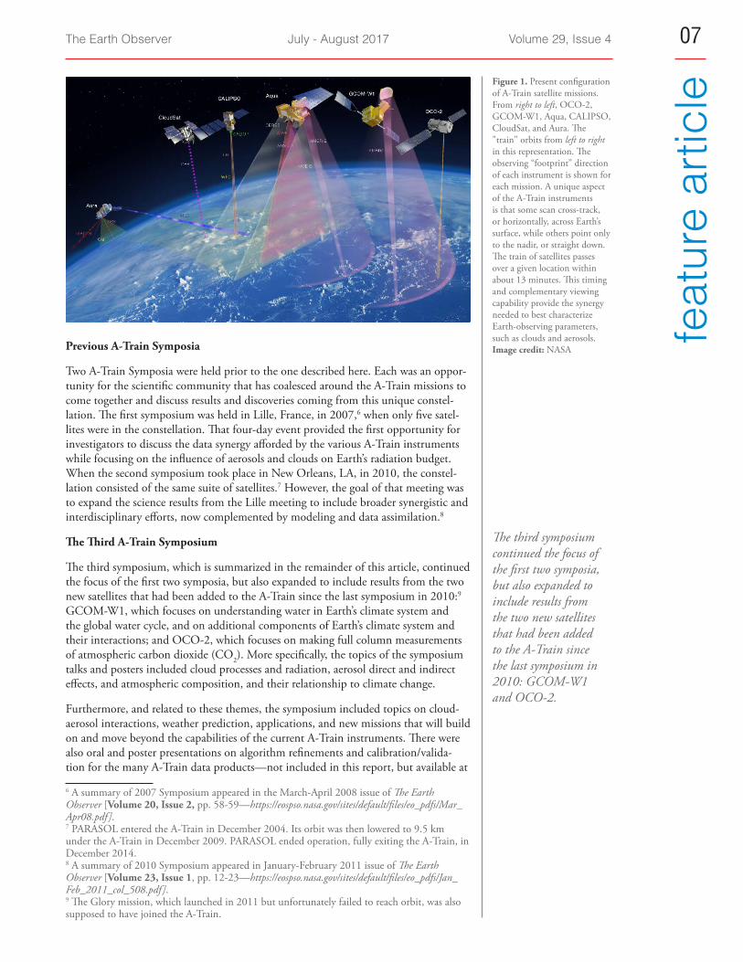
In 2002 as NASA’s Aqua mission prepared for launch, the concept for the Afternoon Constellation was born. It was a similar idea to the Morning Constellation, but this would be a grouping of satellites with a ~1:30 PM (and also ~1:30 AM) local time equator crossing time. The A-Train, as it soon became known, would be a more ambi-tious engineering and logistical feat because it involved the coordination of more satellites than the Morning Constellation—and also would eventually require care-fully planned collaboration with two international partners. Table 1 lists all satellites that are and have been part of the A-Train, when they joined the constellation, their instrument complements, and the science measurement for each. Figure 1 illustrates the current A-Train formation and its six satellites. Many more details on the A-Train and the missions that comprise it can be found at https://atrain.gsfc.nasa.gov. Please note that missions and instruments described later in the text may be referenced by their names, abbreviations, or acronyms. We ask the reader to refer (back) to this table for relevant details when encountering such references.

3 For more on how the EOS concept evolved over a series of “re”-assessments during the early-to-mid 1990s, see “A Washington Parable: EOS in the Context of Mission to Planet Earth” in the March–April 2009 issue of The Earth Observer [Volume 23, Issue 3, pp. 4-12—https://eospso.nasa.gov/sites/default/files/eo_pdfs/May_June_2011_col_508.pdf].4 A good reference for more information on constellation flying, and on NASA’s Morning and Afternoon Constellations, is “Earth Science Mission Operations…Orchestrating NASA’s Fleet of Earth Observing Satellites” in the March–April 2016 issue of The Earth Observer [Volume 28, Issue 2, pp. 4-13—https://eospso.nasa.gov/sites/default/files/eo_pdfs/Mar_Apr_2016_508_color.pdf].5 As of today, Landsats 7 and 8 and Terra remain in the Morning Constellation; the SAC-C mis-sion ended in 2013, and EO-1 was decommissioned in 2016. Landsat 5, which had been in orbit since 1984, also became part of the Morning Constellation until the mission ended in 2013.

In 1999, the Project Scientists for NASA’s Terra mission and the joint NASA–U.S. Geological Survey (USGS) Landsat -7 mission (both preparing for launch at the time) signed an agreement to do what they called “loose formation flying.”

The Earth Observer July - August 2017 Volume 29, Issue 406fe

atur

e ar

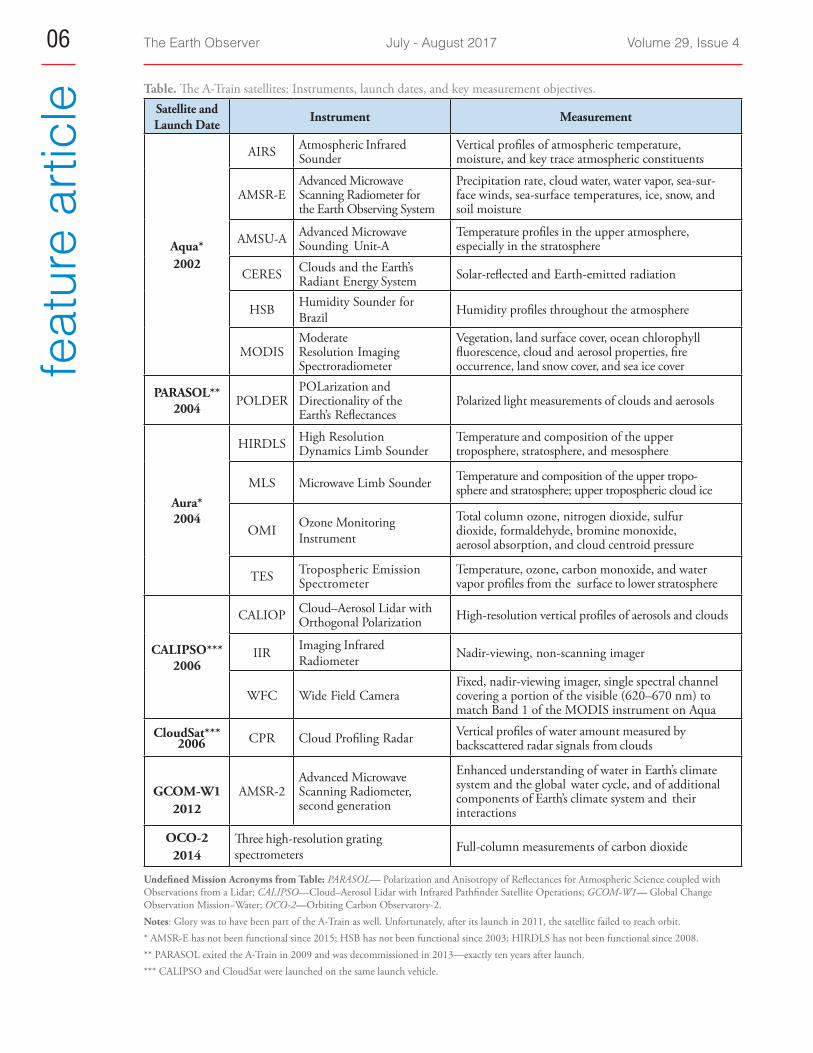
ticle Table. The A-Train satellites: Instruments, launch dates, and key measurement objectives.

Satellite and Launch Date Instrument Measurement

Aqua*2002

AIRS Atmospheric Infrared Sounder

Vertical profiles of atmospheric temperature, moisture, and key trace atmospheric constituents

AMSR-EAdvanced Microwave Scanning Radiometer for the Earth Observing System

Precipitation rate, cloud water, water vapor, sea-sur-face winds, sea-surface temperatures, ice, snow, and soil moisture

AMSU-A Advanced Microwave Sounding Unit-A

Temperature profiles in the upper atmosphere, especially in the stratosphere

CERES Clouds and the Earth’s Radiant Energy System Solar-reflected and Earth-emitted radiation

HSB Humidity Sounder for Brazil Humidity profiles throughout the atmosphere

MODISModerate Resolution Imaging Spectroradiometer

Vegetation, land surface cover, ocean chlorophyll fluorescence, cloud and aerosol properties, fire occurrence, land snow cover, and sea ice cover

PARASOL** 2004 POLDER

POLarization and Directionality of the Earth’s Reflectances

Polarized light measurements of clouds and aerosols

Aura* 2004

HIRDLS High Resolution Dynamics Limb Sounder

Temperature and composition of the upper troposphere, stratosphere, and mesosphere

MLS Microwave Limb Sounder Temperature and composition of the upper tropo-sphere and stratosphere; upper tropospheric cloud ice

OMI Ozone Monitoring Instrument

Total column ozone, nitrogen dioxide, sulfur dioxide, formaldehyde, bromine monoxide, aerosol absorption, and cloud centroid pressure

TES Tropospheric Emission Spectrometer

Temperature, ozone, carbon monoxide, and water vapor profiles from the surface to lower stratosphere

CALIPSO*** 2006

CALIOP Cloud–Aerosol Lidar with Orthogonal Polarization High-resolution vertical profiles of aerosols and clouds

IIR Imaging Infrared Radiometer Nadir-viewing, non-scanning imager

WFC Wide Field CameraFixed, nadir-viewing imager, single spectral channel covering a portion of the visible (620–670 nm) to match Band 1 of the MODIS instrument on Aqua

CloudSat*** 2006 CPR Cloud Profiling Radar Vertical profiles of water amount measured by

backscattered radar signals from clouds

GCOM-W12012

AMSR-2Advanced Microwave Scanning Radiometer, second generation

Enhanced understanding of water in Earth’s climate system and the global water cycle, and of additional components of Earth’s climate system and their interactions

OCO-22014

Three high-resolution grating spectrometers Full-column measurements of carbon dioxide

Undefined Mission Acronyms from Table: PARASOL— Polarization and Anisotropy of Reflectances for Atmospheric Science coupled with Observations from a Lidar; CALIPSO—Cloud–Aerosol Lidar with Infrared Pathfinder Satellite Operations; GCOM-W1— Global Change Observation Mission–Water; OCO-2—Orbiting Carbon Observatory-2.Notes: Glory was to have been part of the A-Train as well. Unfortunately, after its launch in 2011, the satellite failed to reach orbit. * AMSR-E has not been functional since 2015; HSB has not been functional since 2003; HIRDLS has not been functional since 2008.** PARASOL exited the A-Train in 2009 and was decommissioned in 2013—exactly ten years after launch. *** CALIPSO and CloudSat were launched on the same launch vehicle.

The Earth Observer July - August 2017 Volume 29, Issue 4 07

feat

ure

artic

le

Previous A-Train Symposia

Two A-Train Symposia were held prior to the one described here. Each was an oppor-tunity for the scientific community that has coalesced around the A-Train missions to come together and discuss results and discoveries coming from this unique constel-lation. The first symposium was held in Lille, France, in 2007,6 when only five satel-lites were in the constellation. That four-day event provided the first opportunity for investigators to discuss the data synergy afforded by the various A-Train instruments while focusing on the influence of aerosols and clouds on Earth’s radiation budget. When the second symposium took place in New Orleans, LA, in 2010, the constel-lation consisted of the same suite of satellites.7 However, the goal of that meeting was to expand the science results from the Lille meeting to include broader synergistic and interdisciplinary efforts, now complemented by modeling and data assimilation.8

The Third A-Train Symposium

The third symposium, which is summarized in the remainder of this article, continued the focus of the first two symposia, but also expanded to include results from the two new satellites that had been added to the A-Train since the last symposium in 2010:9 GCOM-W1, which focuses on understanding water in Earth’s climate system and the global water cycle, and on additional components of Earth’s climate system and their interactions; and OCO-2, which focuses on making full column measurements of atmospheric carbon dioxide (CO2). More specifically, the topics of the symposium talks and posters included cloud processes and radiation, aerosol direct and indirect effects, and atmospheric composition, and their relationship to climate change.

Furthermore, and related to these themes, the symposium included topics on cloud-aerosol interactions, weather prediction, applications, and new missions that will build on and move beyond the capabilities of the current A-Train instruments. There were also oral and poster presentations on algorithm refinements and calibration/valida-tion for the many A-Train data products—not included in this report, but available at

6 A summary of 2007 Symposium appeared in the March-April 2008 issue of The Earth Observer [Volume 20, Issue 2, pp. 58-59—https://eospso.nasa.gov/sites/default/files/eo_pdfs/Mar_Apr08.pdf].7 PARASOL entered the A-Train in December 2004. Its orbit was then lowered to 9.5 km under the A-Train in December 2009. PARASOL ended operation, fully exiting the A-Train, in December 2014.8 A summary of 2010 Symposium appeared in January-February 2011 issue of The Earth Observer [Volume 23, Issue 1, pp. 12-23—https://eospso.nasa.gov/sites/default/files/eo_pdfs/Jan_Feb_2011_col_508.pdf].9 The Glory mission, which launched in 2011 but unfortunately failed to reach orbit, was also supposed to have joined the A-Train.

The third symposium continued the focus of the first two symposia, but also expanded to include results from the two new satellites that had been added to the A-Train since the last symposium in 2010: GCOM-W1 and OCO-2.

Figure 1. Present configuration of A-Train satellite missions. From right to left, OCO-2, GCOM-W1, Aqua, CALIPSO, CloudSat, and Aura. The "train" orbits from left to right in this representation. The observing “footprint” direction of each instrument is shown for each mission. A unique aspect of the A-Train instruments is that some scan cross-track, or horizontally, across Earth’s surface, while others point only to the nadir, or straight down. The train of satellites passes over a given location within about 13 minutes. This timing and complementary viewing capability provide the synergy needed to best characterize Earth-observing parameters, such as clouds and aerosols. Image credit: NASA

The Earth Observer July - August 2017 Volume 29, Issue 408fe

atur

e ar

ticle https://atrain2017.org/presentations. Aqua, the first constellation satellite, was launched

in 2002, and several of the A-Train missions are now showing their functional age, so an informal report on A-Train flight operations management and the future of the constellation was of particular interest to the attendees.

The very busy three-day symposium included 60 presentations and over 150 poster papers. The event began with representatives from NASA Headquarters (HQ) manage-ment on the status of funding and future opportunities in Earth science research. Two keynote presentations on the challenges for upcoming Earth system science measure-ments and the economic value of climate observations were highlights of the symposium. Summarizing every paper in this brief article is not possible because of space limitations; therefore, only symposium theme highlights and programmatic topics are presented here. Most presentations and poster papers can be found at the A-Train URL listed above.

Management Perspective: Status and Opportunities

Hal Maring [NASA Headquarters (HQ)—Radiation Sciences Program Manager, A-Train Program Scientist] greeted the attendees and discussed the overall future of A-Train operations and its member missions. He pointed out that there would be future in-orbit maneuvers by the member missions to maintain their science require-ments and adjustments as satellite fuel, needed to maintain formation, is depleted. Maring encouraged the mission scientists to determine how to manage the A-Train for-mation in light of the fact that the Chinese TanSat mission—a carbon dioxide-measur-ing satellite launched in December 2016—will periodically fly very close to the A-Train satellites, and could potentially result in a safety concern for the constellation. Finally, he discussed upcoming requirements and opportunities for A-Train mission science analysis, emphasizing the benefits that would derive from multidisciplinary approaches.

Jack Kaye [NASA HQ—Associate Director for Research of the Earth Science Division] continued the programmatic discussion with a review of the impor-tance of the A-Train research in NASA’s Earth-observation program, and how the activities of U.S. government agencies and international Earth science missions complement the capabilities of the A-Train. Kaye highlighted NASA’s collabora-tion with international environmental working groups such as the United Nations Environment Programme (UNEP), the World Meteorological Organization (WMO), and the Intergovernmental Panel on Climate Change (IPCC).10 He also acknowledged the participation of the many scientists in NASA’s peer review pro-cess in maintaining high-quality science. He ended with a broad overview of Earth science funding sources and encouraged optimism, as budget negotiations were underway at that time.

Keynote Presentations: Value and Challenges for Climate Research

Keynote presentations by two senior A-Train scientists are summarized below to pro-vide context for the overall symposium theme discussions that follow.

Graeme Stephens [NASA/Jet Propulsion Laboratory (JPL)—Director of the Center for Climate Sciences, CloudSat Principal Investigator] focused on how the A-Train’s success points to a bright future for continued Earth observations and their impact on climate research—e.g., see Moving Beyond the A-Train: EarthCare and Other New Measurements on page 17. He spoke about how the A-Train enabled new science achievements and made multidisciplinary science possible. Stephens defined the chal-lenge of Earth system science as “explaining the past, understanding the present, and predicting the future.” He described how observations of Earth system science enable prediction of future climate change. On the other hand, data from observa-tions also reveal key biases in community climate models of the Earth system. These biases result from several factors including uncertainties in: sea surface temperatures, 10 The IPCC was established in 1988 by the WMO and the UNEP to assess scientific, technical and socioeconomic information concerning climate change, its potential effects, and options for adaptation and mitigation. The IPCC has issued a series of reports since 1990; the most recent was the fifth Assessment Report (AR-5), released in 2013.

Two keynote presentations on the challenges for upcoming Earth system science measurements and the economic value of climate observations were highlights of the symposium.

The Earth Observer July - August 2017 Volume 29, Issue 4 09

feat

ure

artic

levertical structure and distribution of cloud types, precipitation amounts, effects of vol-canic eruptions, and treatment of the El Niño–Southern Oscillation (ENSO).11 For the future, there is a consensus in the science community that an integrated and bal-anced measurement strategy is needed using lower-cost measurement systems flying in a constellation, and that science themes should focus on processes more than just individual environmental parameters—a key change in approach, but one that could only have arisen from lessons learned from earlier approaches. Stephens concluded by summarizing how the National Academy’s 2017 Decadal Survey for Earth Science and Applications from Space (ESAS)12 is formulating consensus recommendations from the Earth science and applications communities for future missions.

Bruce Wielicki [NASA’s Langley Research Center (LaRC)—Science Team Lead for the Climate Absolute Radiance and Refractivity Observatory (CLARREO) Mission] gave the second keynote address, which was titled “Economic Value of a New Climate Observing System.” He began by showing how the value of climate science observa-tions might be estimated. Wielicki stated that the use of integrative assessment mod-els (IAMs) is the mainstream methodological approach in climate change research, and that such models rely on climate change disciplines, involve social-economic components as well as natural sciences components, and can then be used for sce-nario designs. The model can define measurement accuracy requirements for a climate observing system based on the measurement period for detecting climate change, natural variability, and the magnitude of human driven climate change. The accuracy of the system will then drive measurement system cost. Wielicki ended with a demon-stration that showed that long-term measurements of shortwave cloud radiative forc-ing as a climate sensitivity trigger would be more cost effective (by a factor of two) than using a temperature trigger.

Climate Science: Models Benefit from Data

Earth’s energy balance, or the idea that the radiant solar energy absorbed by the Earth must equal the energy it radiates back to space, which was once thought to be a fun-damental constraint on the climate system.

A revised planetary energy balance framework was suggested, where the top of the atmosphere (TOA) net radiation is parameterized in terms of 500-hPa tropical tem-perature instead of surface temperature. Model estimates of climate sensitivity (ECS)13 based upon the CERES short-term data record compared to estimates that used the “old” framework using surface warming yields a lower ECS than measurements, but is within the IPCC lower range.

The new energy balance formulation is also less impacted by internal climate variabil-ity, which may substantially bias previous estimates of ECS derived from historical observations of surface warming. Using the new framework, the observations suggest ECS is likely below the current 3.5-K (6.3-°F) estimate, but is within the IPCC’s AR5 report range. That it falls in the lower end of this range provides some support that models can be further constrained.

Uncertainty in model predictions of ECS result from differences in various parameters, e.g., the extent to which precipitation would change under conditions of increased or continued global warming. In this example, the atmospheric longwave radiative cooling rate predominantly controls global mean precipitation, and is a function of cloud cover. A decrease of high cloud cover leads to increased precipitation because of enhanced longwave radiation loss to space. Analyses using CERES radiative flux measurements

11 ENSO is an irregularly periodical variation in winds and sea surface temperatures over the tropical eastern Pacific Ocean, which has impacts on weather patterns around the globe.12 To learn more about plans for the 2017 Decadal Survey, visit http://sites.nationalacademies.org/DEPS/ESAS2017/index.htm.13 The term climate sensitivity is often used to specify the equilibrium global mean surface tem-perature change that results from a doubling of atmospheric CO2 concentration. However, in this context it is being applied more broadly as a metric to characterize the response of the global climate system to a given forcing.

A revised planetary energy balance framework was suggested, where the top of the atmosphere (TOA) net radiation is parameterized in terms of 500-hPa tropical temperature instead of surface temperature.

The Earth Observer July - August 2017 Volume 29, Issue 410fe

atur

e ar

ticle with MODIS and CALIPSO cloud fraction and water vapor data showed that most

climate models underestimate the decrease of tropical high cloud cover with increasing surface temperature. Therefore, models underestimate precipitation increase because of their deficiencies in simulating tropical circulation—particularly the Hadley circulation.14 This result will provide a pathway to improve model predictions of how rainfall patterns will change in response to global warming.

Another study that was described during this session showed that current cloud clima-tologies, used in climate models, tend to miss optically thin and multilayer clouds or misrepresent the altitudes of these clouds. The errors arise because these climatologies are based on passive measurements, which are often confounded by physical, chemi-cal, and process-oriented complexities of the real atmosphere and thus cannot reveal the vertical distribution of clouds. Such information is critically important for accu-rately portraying deep convection in models, as well as constructing accurate heating rate profiles. Clouds, coupled circulation, and subsequent feedbacks are still highly parameterized in most current estimates of cloud characteristics, and this leads to uncertainties in determining climate sensitivity.

Several presentations during the session focused on one or more cloud properties and how they contribute to the energy balance at the top of the atmosphere. Most of these studies concentrated on the tropics, using various combinations of A-Train measure-ments. For example, one presentation described efforts to track upper tropospheric cloud systems feedback using observations from AIRS in synergy with those from AMSR-E, CALIPSO, and CloudSat. In another case, the researchers used CALIPSO opacity observations to provide new constraints on cloud–radiation interaction. Still another presentation made a convincing case that some climate models significantly underestimate thin or broken cloud cover.

There was additional discussion about responses to climate change during which it was noted that, in recent years, the strongest response to climate change is taking place in the Arctic. Along those lines, there were several presentations on the decline in areal extent and thickness of Arctic sea ice. In addition to increasing air temperature, winter precondition phenomena—which include water vapor, cloudiness, and circula-tion changes—account for a significant fraction of the variability in September sea ice extent from the observed long-term downward trend. Since the decline in Arctic sea ice has increased most rapidly during the lifetime of AIRS, its measurements provide an ideal dataset to gain a better understanding of the complex sea ice-ocean-atmo-sphere interactions occurring in that region. The AIRS data show surface temperatures warming at twice the rate of air temperatures—particularly in fall and winter. Large uncertainties are found in moisture flux, or evaporation, and interactions with the sur-face and low-level clouds. Consequently, these clouds appear to be increasing.

The influence of climate change on regional phenomena, such as weather and global-scale events is difficult to explain, but a possible connection came from an analysis of Aura/MLS, CALIPSO, and aircraft radar observations, which were used to analyze the unusual weather pattern over North America during the winter of 2015–2016. Concurrently, there were anomalously warm sea surface temperatures (SST) in the central Pacific and a shift in convection intensity from the western- to the central-Pacific, with large amounts of cloud-ice near the tropopause leading to increased water vapor in the lower stratosphere. There was even an abrupt change in the usually regu-lar quasibiennial oscillation (QBO)15 of the winds in the lower stratosphere. The data seem to show a connection between increased SST and changes in the upper tropo-sphere cloud-ice levels, resulting in increased water vapor levels due to enhanced con-vection. This result showed that increasing lower stratospheric water vapor increases surface temperature and becomes a positive feedback to climate change.14 The Hadley circulation is a global scale tropical atmospheric phenomenon in which air rises near the equator, flows poleward at 10–15 km above the surface, descends in the subtropics, and then returns equatorward near the surface.15 QBO is a quasiperiodic oscillation of the equatorial zonal wind between easterlies and wester-lies in the tropical stratosphere with a mean period of 28 to 29 months. 

Since the decline in Arctic sea ice has increased most rapidly during the lifetime of AIRS, its measurements provide an ideal dataset to gain a better understanding of the complex sea ice-ocean-atmosphere interactions occurring in that region.

The Earth Observer July - August 2017 Volume 29, Issue 4 11

feat

ure

artic

leCloud Physics and Radiation

Clouds are one of the critical “control knobs” for climate models. The IPCC AR5 report reiterated that clouds remain the largest source of uncertainty in climate pro-jections. Therefore, their influence on climate was a key theme for the symposium. The major sources for cloud data used for the presentations in this session came from CloudSat and CALIPSO; however, several other A-Train instruments provided neces-sary complementary data.

Despite the uncertainties mentioned above, the IPCC AR5 has acknowledged that A-Train instruments enhance the accuracy of climate model processes because of their ability to vertically resolve cloud information through a combination of passive and active sensors. Over the last 10 years, CALIPSO and CloudSat have characterized the current state and interannual variability of clouds. However, challenges remain with complementary models and climatologies. There is general agreement that cur-rent uncertainties in climate sensitivity are largely due to uncertainties in modeling cloud–radiation–climate feedbacks. The nature and extent of these complex feedbacks are uncertain because they are a function of cloud height, cloud cover, and optical depth. However, current measurements from the A-Train, as well as those anticipated from upcoming missions—see Moving beyond the A-Train on page 17—have the accu-racy and stability needed to monitor cloud characteristic changes over the long term, which will enable observation of their respective responses to climate warming.

Cloud-type distributions vary seasonally and interannually as a function of solar radia-tion, large-scale atmospheric dynamics, and thermodynamics, which, in turn, regulate the global water and energy cycles. Climate changes can result in changing frequency of a particular cloud type and its distribution, and the combination of these determines cloud feedbacks. A study of 10-year combined CloudSat and CALIPSO cloud-type data products were used to check how well climate models capture the key variations. As an example, the study showed how the Walker circulation16 affected the locations of tropical deep convective clouds, which also shift with the seasons. On interannual scales, ENSO had the effect of shifting the longitude of convective centers.

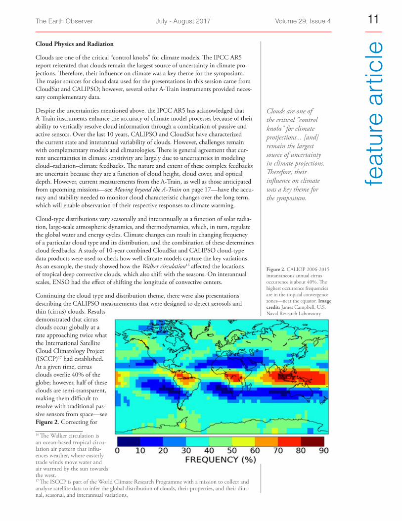
Continuing the cloud type and distribution theme, there were also presentations describing the CALIPSO measurements that were designed to detect aerosols and thin (cirrus) clouds. Results demonstrated that cirrus clouds occur globally at a rate approaching twice what the International Satellite Cloud Climatology Project (ISCCP)17 had established. At a given time, cirrus clouds overlie 40% of the globe; however, half of these clouds are semi-transparent, making them difficult to resolve with traditional pas-sive sensors from space—see Figure 2. Correcting for

16 The Walker circulation is an ocean-based tropical circu-lation air pattern that influ-ences weather, where easterly trade winds move water and air warmed by the sun towards the west.17 The ISCCP is part of the World Climate Research Programme with a mission to collect and analyze satellite data to infer the global distribution of clouds, their properties, and their diur-nal, seasonal, and interannual variations.

Figure 2. CALIOP 2006-2015 instantaneous annual cirrus occurrence is about 40%. The highest occurrence frequencies are in the tropical convergence zones—near the equator. Image credit: James Campbell, U.S. Naval Research Laboratory

Clouds are one of the critical "control knobs" for climate protjections... [and] remain the largest source of uncertainty in climate projections. Therefore, their influence on climate was a key theme for the symposium.

The Earth Observer July - August 2017 Volume 29, Issue 412fe

atur

e ar

ticle unresolved thin cirrus, CALIPSO measurements showed global cloudiness is about

74%, which is in close agreement with ISCCP total global cloudiness, reported as being in the 60-70% range. These measurements provide a more thorough under-standing of how cirrus clouds affect the Earth radiation budget overall.

CERES, CloudSat, CALIPSO, and MODIS data were combined to examine the struc-ture of clouds that maintain the radiative balance in tropical convective zones. The net radiative neutrality of tropical convective clouds is a product of the structure and life-cycle of organized tropical convection. Top-of-the-atmosphere neutrality (i.e., balance in the Earth’s radiation budget) was also shown to be related to the relative abundance of thick versus thin anvil clouds and the life cycle of the anvil cloud produced by tropi-cal convection. This net balance is possible because rainy cores and thick anvils produce a net negative radiative effect, but then they spread out (becoming thinner) and rise to produce a large area of cloud that has a positive net radiative effect.

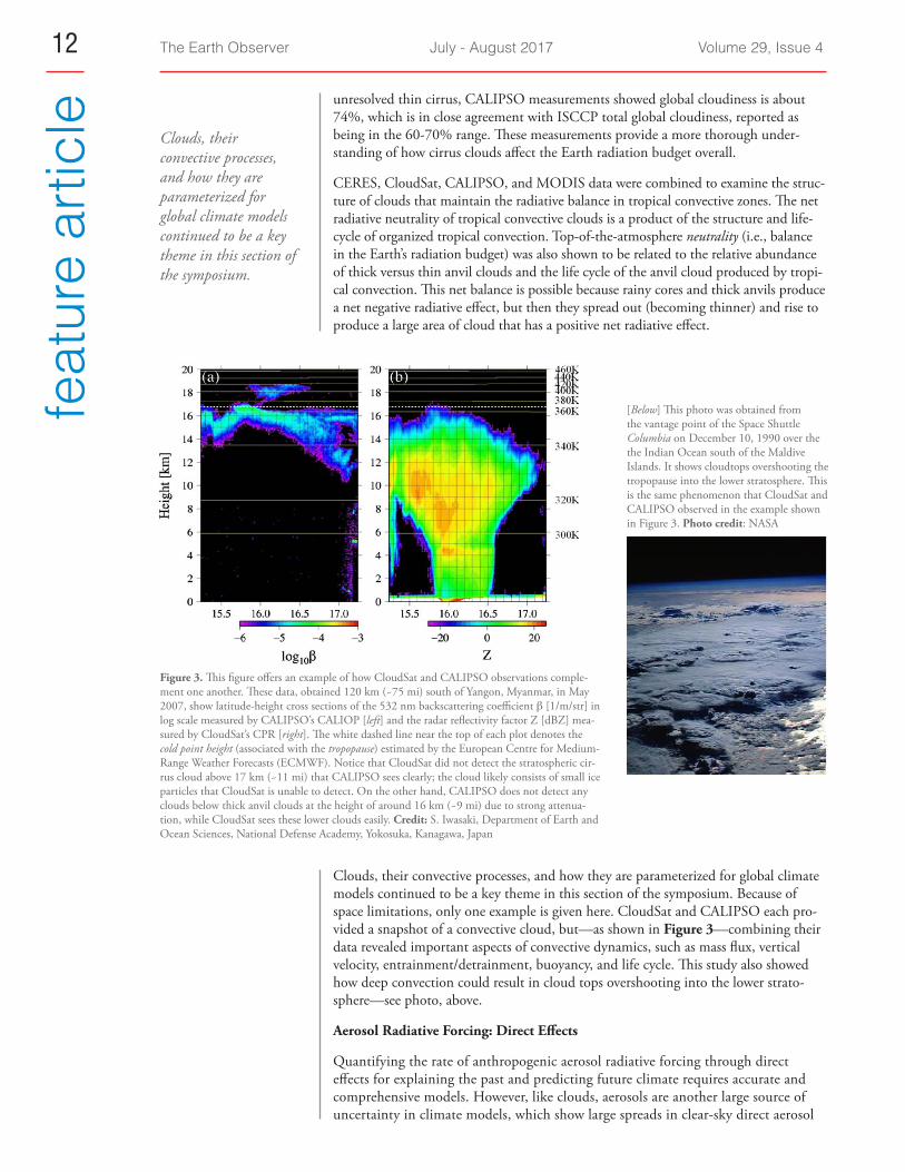
[Below] This photo was obtained from the vantage point of the Space Shuttle Columbia on December 10, 1990 over the the Indian Ocean south of the Maldive Islands. It shows cloudtops overshooting the tropopause into the lower stratosphere. This is the same phenomenon that CloudSat and CALIPSO observed in the example shown in Figure 3. Photo credit: NASA

Figure 3. This figure offers an example of how CloudSat and CALIPSO observations comple-ment one another. These data, obtained 120 km (~75 mi) south of Yangon, Myanmar, in May 2007, show latitude-height cross sections of the 532 nm backscattering coefficient β [1/m/str] in log scale measured by CALIPSO’s CALIOP [left] and the radar reflectivity factor Z [dBZ] mea-sured by CloudSat’s CPR [right]. The white dashed line near the top of each plot denotes the cold point height (associated with the tropopause) estimated by the European Centre for Medium-Range Weather Forecasts (ECMWF). Notice that CloudSat did not detect the stratospheric cir-rus cloud above 17 km (~11 mi) that CALIPSO sees clearly; the cloud likely consists of small ice particles that CloudSat is unable to detect. On the other hand, CALIPSO does not detect any clouds below thick anvil clouds at the height of around 16 km (~9 mi) due to strong attenua-tion, while CloudSat sees these lower clouds easily. Credit: S. Iwasaki, Department of Earth and Ocean Sciences, National Defense Academy, Yokosuka, Kanagawa, Japan

Clouds, their convective processes, and how they are parameterized for global climate models continued to be a key theme in this section of the symposium. Because of space limitations, only one example is given here. CloudSat and CALIPSO each pro-vided a snapshot of a convective cloud, but—as shown in Figure 3—combining their data revealed important aspects of convective dynamics, such as mass flux, vertical velocity, entrainment/detrainment, buoyancy, and life cycle. This study also showed how deep convection could result in cloud tops overshooting into the lower strato-sphere—see photo, above.

Aerosol Radiative Forcing: Direct Effects

Quantifying the rate of anthropogenic aerosol radiative forcing through direct effects for explaining the past and predicting future climate requires accurate and comprehensive models. However, like clouds, aerosols are another large source of uncertainty in climate models, which show large spreads in clear-sky direct aerosol

Clouds, their convective processes, and how they are parameterized for global climate models continued to be a key theme in this section of the symposium.

The Earth Observer July - August 2017 Volume 29, Issue 4 13

ticle

e ar

feat

ur

radiative forcing. Efforts to resolve this uncertainty have motivated many studies on aerosol composition, optical characteristics, and their temporal and spatial changes, a number of which were described during this session. After being run, models must be tested using observations such as those from the A-Train to constrain aerosol radiative properties. One example of such an effort described during the symposium showed that comparisons of model and measurement-derived direct radiative effects exhibit a seasonal bias, with measurement sampling error likely being one of the causes.

In another study to reconcile measurements and models, the researchers compared aerosol optical depth (AOD) and absorbing aerosol optical depth (AAOD) from dif-ferent sources. Absorbing aerosols play a role in cloud formation through aerosol-cloud interactions (discussed below in the Aerosol Indirect Effects section). Most of these aerosols are black carbon and organic particles produced by human activities, although dust originating from arid land areas is also included. Important as they are, global observations of these aerosols remain sparse. The study compared data from the A-Train (PARASOL and Aura/OMI) with data from atmospheric chem-istry models (GOCART18 and GEOS-519), supplemented with information from the Modern-Era Retrospective Analysis for Research and Applications (MERRA).20 Specifically, the comparisons were conducted over Aerosol Robotic Network (AERONET) sites located in regions with heavy aerosol concentrations and in rela-tively “clean” areas with few aerosol sources. Results were mixed, depending on aero-sol types and their local sources (e.g., land, coastal, ocean) pointing to the need for better instrument discrimination and sensitivity and more-accurate aerosol optical property parameterizations to improve model calculations.

The Asian tropopause aerosol layer, a dominating and recurring feature associated with the Asian Monsoon, has been studied extensively with ground-based, bal-loon, aircraft, and satellite data. These measurements showed the aerosols that make up this layer are small, mostly volatile, and composed of a combination of sulfate and organic materials that appear to originate in eastern China and northern India. Another study over the southeast Atlantic region that used data from a variety of A-Train instruments and from the Cloud-Aerosol Transport System (CATS) mounted on the International Space Station (ISS) revealed that the aerosol layer from smoke is much closer to underlying clouds than that shown by CALIPSO. This implies that microphysical processes will have an impact on the direct radiative effect, and that it may have a diurnal component, which—unlike CALIPSO—CATS can observe from its van-tage point on the ISS.

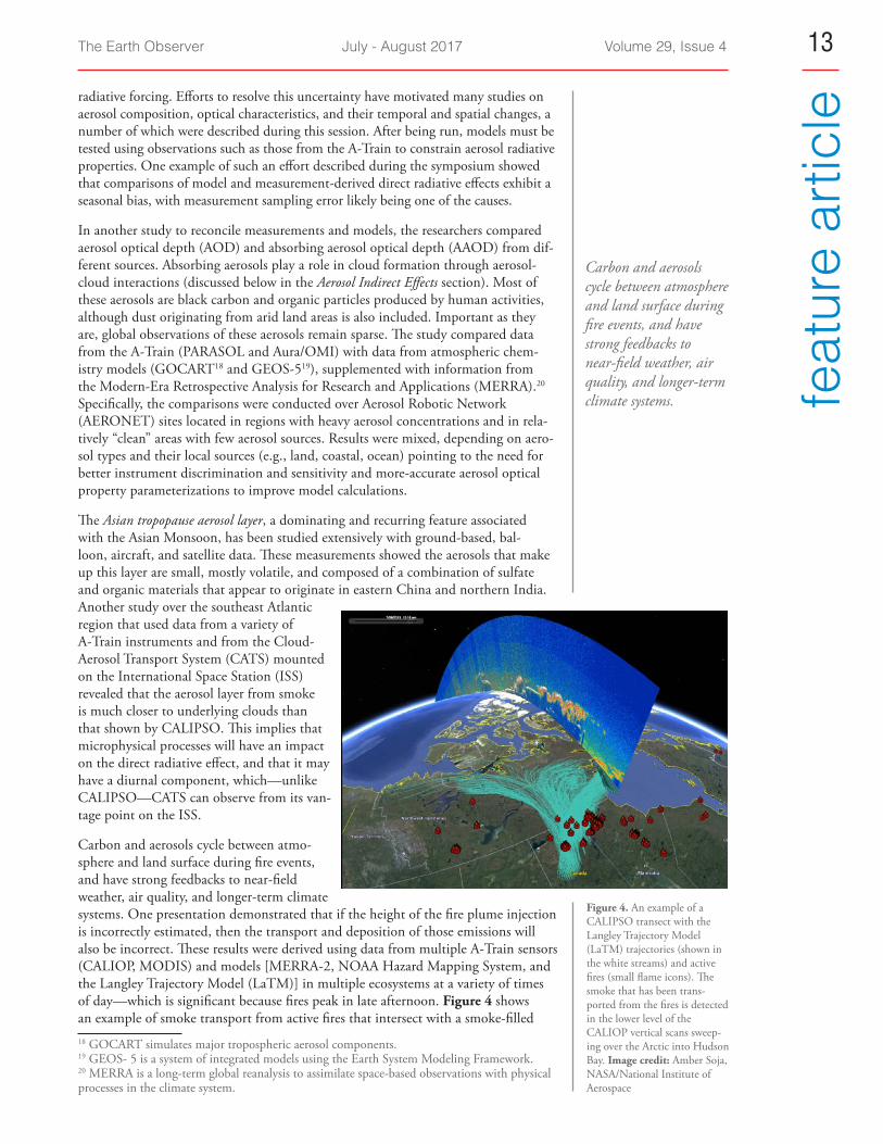
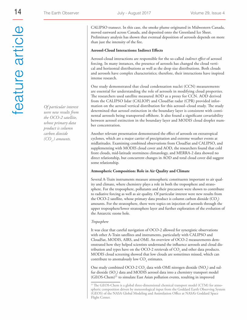
Carbon and aerosols cycle between atmo-sphere and land surface during fire events, and have strong feedbacks to near-field weather, air quality, and longer-term climate systems. One presentation demonstrated that if the height of the fire plume injection is incorrectly estimated, then the transport and deposition of those emissions will also be incorrect. These results were derived using data from multiple A-Train sensors (CALIOP, MODIS) and models [MERRA-2, NOAA Hazard Mapping System, and the Langley Trajectory Model (LaTM)] in multiple ecosystems at a variety of times of day—which is significant because fires peak in late afternoon. Figure 4 shows an example of smoke transport from active fires that intersect with a smoke-filled 18 GOCART simulates major tropospheric aerosol components.19 GEOS- 5 is a system of integrated models using the Earth System Modeling Framework.20 MERRA is a long-term global reanalysis to assimilate space-based observations with physical processes in the climate system.

Figure 4. An example of a CALIPSO transect with the Langley Trajectory Model (LaTM) trajectories (shown in the white streams) and active fires (small flame icons). The smoke that has been trans-ported from the fires is detected in the lower level of the CALIOP vertical scans sweep-ing over the Arctic into Hudson Bay. Image credit: Amber Soja, NASA/National Institute of Aerospace

Carbon and aerosols cycle between atmosphere and land surface during fire events, and have strong feedbacks to near-field weather, air quality, and longer-term climate systems.

The Earth Observer July - August 2017 Volume 29, Issue 414fe

atur

e ar

ticle CALIPSO transect. In this case, the smoke plume originated in Midwestern Canada,

moved eastward across Canada, and deposited onto the Greenland Ice Sheet. Preliminary analysis has shown that eventual deposition of aerosols depends on more than just the intensity of the fire.

Aerosol-Cloud Interactions: Indirect Effects

Aerosol-cloud interactions are responsible for the so-called indirect effect of aerosol forcing. In many instances, the presence of aerosols has changed the cloud verti-cal and horizontal distributions as well as the drop size distributions. Both clouds and aerosols have complex characteristics; therefore, their interactions have inspired intense research.

One study demonstrated that cloud condensation nuclei (CCN) measurements are essential for understanding the role of aerosols in modifying cloud properties. The researchers used satellite measured AOD as a proxy for CCN. AOD derived from the CALIPSO lidar (CALIOP) and CloudSat radar (CPR) provided infor-mation on the aerosol vertical distribution for this aerosol–cloud study. The study determined that aerosol extinction in the boundary layer is consistent with conti-nental aerosols being transported offshore. It also found a significant covariability between aerosol extinction in the boundary layer and MODIS cloud droplet num-ber concentration.

Another relevant presentation demonstrated the effect of aerosols on extratropical cyclones, which are a major carrier of precipitation and extreme weather events at midlatitudes. Examining combined observations from CloudSat and CALIPSO, and supplementing with MODIS cloud cover and AOD, the researchers found that cold front clouds, mid-latitude storminess climatology, and MERRA-2 data showed no direct relationship, but concurrent changes in AOD and total cloud cover did suggest some relationship.

Atmospheric Composition: Role in Air Quality and Climate

Several A-Train instruments measure atmospheric constituents important to air qual-ity and climate, where chemistry plays a role in both the troposphere and strato-sphere. For the troposphere, pollutants and their precursors were shown to contribute to radiative forcing as well as air quality. Of particular interest were new results from the OCO-2 satellite, whose primary data product is column carbon dioxide (CO2) amounts. For the stratosphere, there were topics on injection of aerosols through the upper troposphere/lower stratosphere layer and further exploration of the evolution of the Antarctic ozone hole.

Troposphere

It was clear that careful navigation of OCO-2 allowed for synergistic observations with other A-Train satellites and instruments, particularly with CALIPSO and CloudSat, MODIS, AIRS, and OMI. An overview of OCO-2 measurements dem-onstrated how they helped scientists understand the influence aerosols and cloud dis-tribution and types have on the OCO-2 retrievals of CO2 and other data products. MODIS cloud screening showed that low clouds are sometimes missed, which can contribute to anomalously low CO2 estimates.

One study combined OCO-2 CO2 data with OMI nitrogen dioxide (NO2) and sul-fur dioxide (SO2) data and MODIS aerosol data into a chemistry transport model (GEOS-Chem)21 to simulate East Asian pollution events, resulting in improved

21 The GEOS-Chem is a global three-dimensional chemical transport model (CTM) for atmo-spheric composition driven by meteorological input from the Goddard Earth Observing System (GEOS) of the NASA Global Modeling and Assimilation Office at NASA’s Goddard Space Flight Center.

Of particular interest were new results from the OCO-2 satellite, whose primary data product is column carbon dioxide (CO2 ) amounts.

The Earth Observer July - August 2017 Volume 29, Issue 4 15

feat

ure

artic

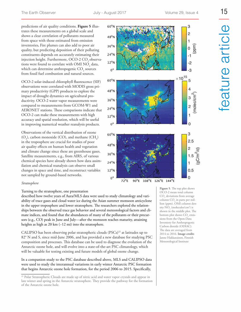
lepredictions of air quality conditions. Figure 5 illus-trates these measurements on a global scale and shows a clear correlation of pollutants measured from space with those estimated from emission inventories. Fire plumes can also add to poor air quality, but predicting deposition of their polluting constituents depends on accurately estimating their injection height. Furthermore, OCO-2 CO2 observa-tions were found to correlate with OMI NO2 data, which can determine anthropogenic CO2 sources from fossil fuel combustion and natural sources. 

OCO-2 solar-induced chlorophyll fluorescence (SIF) observations were correlated with MODIS gross pri-mary productivity (GPP) products to explore the impact of drought dynamics on agricultural pro-ductivity. OCO-2 water vapor measurements were compared to measurements from GCOM-W1 and AERONET stations. These comparisons indicate that OCO-2 can make these measurements with high accuracy and spatial resolution, which will be useful in improving numerical weather reanalysis products.

Observations of the vertical distribution of ozone (O3), carbon monoxide (CO), and methane (CH4) in the troposphere are crucial for studies of poor air quality effects on human health and vegetation and climate change since these are greenhouse gases. Satellite measurements, e.g., from AIRS, of various chemical species have already shown how data assim-ilation and chemical reanalysis can observe small changes in space and time, and reconstruct variables not sampled by ground-based networks.

Stratosphere

Turning to the stratosphere, one presentation described how twelve years of Aura/MLS data were used to study climatology and vari-ability of trace gases and cloud water ice during the Asian summer monsoon anticyclone in the upper troposphere and lower stratosphere. The researchers explored the relation-ships between the observed trace gas behavior and several meteorological factors and cli-mate indices, and found that the abundances of many of the pollutants or their precur-sors (e.g., CO) peak in June and July—after the monsoon reaches maturity, attaining heights as high as 20 km (~12 mi) into the stratosphere.

CALIPSO has been observing polar stratospheric clouds (PSCs)22 at latitudes up to 82° N and S, since mid-June 2006, and has provided a new database for studying PSC composition and processes. This database can be used to diagnose the evolution of the Antarctic ozone hole, and will evolve into a state-of-the-art PSC climatology, which will be valuable for testing existing and future models of global ozone change.

In a companion study to the PSC database described above, MLS and CALIPSO data were used to study the interannual variations in early winter Antarctic PSC formation that begins Antarctic ozone hole formation, for the period 2006 to 2015. Specifically,

22 Polar Stratospheric Clouds are made up of nitric acid and water vapor crystals and appear in late winter and spring in the Antarctic stratosphere. They provide the pathway for the formation of the Antarctic ozone hole.

Figure 5. The top plot shows OCO-2 mean total column CO2 deviations from average column CO2 in parts per mil-lion (ppm). OMI column den-sity NO2 (molecules/cm2) is shown in the middle plot. The bottom plot shows CO2 emis-sions from the Open-Data Inventory for Anthropogenic Carbon dioxide (ODIAC). The data are averaged from 2014 to 2016. Image credit: Janne Hakkarainen, Finnish Meteorological Institute

The Earth Observer July - August 2017 Volume 29, Issue 416fe

atur

e ar

ticle the study investigated the MLS nitric acid (HNO3) evolution and distribution that

make up PSCs in the early winter Antarctic vortex, and found that at the very start of the winter, synoptic-scale depletion of HNO3 can be detected in the inner vortex before the first CALIPSO detection of PSCs. 

Weather and Other Applications

A-Train measurements have been tested as operational data for input to numeri-cal weather prediction (NWP) models. For example, tests conducted by the Naval Research Laboratory have shown that assimilation of AIRS radiances into NWP schemes has resulted in a forecast error reduction of 12%. Future satellites flying hyperspectral instruments, with performance similar to or better than CrIS, IASI, and AIRS, will likely improve this result even further. However, aerosol-characteristics data (e.g., from CALIPSO and MODIS) must be properly accounted for, as they can result in significant biases in the temperature profiles used in the predictions.

A Canadian high-resolution global environmental multiscale model for NWP was used to assess the ability to predict high-ice-water content conditions using data from A-Train satellites and in situ aircraft measurements at high altitude for aviation safety. In the case studied, CloudSat retrievals of ice water clouds (IWC) were close to the aircraft in situ measurements except when the IWC density was high. In addition, the high-resolution model showed the potential to predict the tropical deep convective clouds needed for aircraft safety and operations.

In another application, A-Train data were tested against standard indicators used to predict vegetative drought. Early warning of drought is critical to mitigating drought damage to agricultural products, particularly as droughts are expected to become more frequent and intense with climate change. The Vapor Pressure Deficit (VPD) data product provided from AIRS measurements of temperature and relative humid-ity was used with the OCO-2 solar-induced chlorophyll fluorescence (SIF) data prod-uct for two U.S. drought events: in 2012 and 2016. The researchers found that their data improved drought early warnings from U.S. Drought Monitor (USDM) if inte-grated into current operational systems. For these two cases, the use of A-Train data improved the lead times by 100 days (2012) and by 40 days (2016) for drought onset. Having begun in April 2017, the performing team is providing USDM with updated VPD and humidity information every week in a near-real-time (NRT) mode.

A poster paper described new capabilities added to NASA’s Land Atmosphere Near real-time Capability for EOS (LANCE). LANCE supports application users inter-ested in monitoring a wide variety of natural and man-made phenomena in NRT mode, e.g., for fire management, ash plumes, and flooding. Images from AIRS, MLS, MODIS, and OMI are generally available three-to-five hours after observa-tion. Over the last year, LANCE has been enhanced to include NRT products from GCOM-W1/AMSR2, the Multi-angle Imaging SpectroRadiometer (MISR) on Terra, and the Visible Infrared Imaging Radiometer Suite (VIIRS) on the Suomi National Polar-orbiting Partnership (NPP) satellite. In addition, the selection of LANCE NRT imagery can be viewed interactively through Worldview and the Global Imagery Browse Services (GIBS). This year, LANCE will add data from the Ozone Mapping Profiler Suite (OMPS) on Suomi NPP and the Measurement of Pollution in the Troposphere (MOPITT) on Terra. For more information about these capabilities, visit https://earthdata.nasa.gov/lance.

Several other posters further illustrated various applications of A-Train data, including how multiple A-Train instruments and ground-based radars can observe the develop-ment of tornadoes, how sea level pressure can be applied to numerical weather predic-tions and diagnosing the origins of extreme weather, and how knowledge of improved aerosol properties can improve visibility and air-quality forecasts.

The Vapor Pressure Deficit (VPD) data product provided from AIRS measurements of temperature and relative humidity was used with the OCO-2 solar-induced chlorophyll fluorescence (SIF) data product for two U.S. drought events: in 2012 and 2016. They found that their data improved drought early warnings from U.S. Drought Monitor (USDM) if integrated into current operational systems.

The Earth Observer July - August 2017 Volume 29, Issue 4 17

feat

ure

artic

leMoving Beyond the A-Train: EarthCare and Other New MeasurementsSeveral oral presentations and posters described the European Space Agency’s (ESA) implementation of the Earth Cloud, Aerosol and Radiation Explorer (EarthCARE) mission in cooperation with the Japan Aerospace Exploration Agency (JAXA), with launch planned for late 2018. The mission will be in a 2:00 PM local time equator-crossing-time orbit—compared to the A-Train’s 1:30 PM crossing-time—and there-fore will provide synergistic measurements with the A-Train members. The EarthCARE payload consists of two active (radar and lidar) and two passive (imager and radiometer) instruments. The four instruments will provide three-dimensional (3D) cloud-aerosol-precipitation scenes, with collocated broadband radia-tion data over the two-year planned mission lifetime.*

There was discussion about state-of-the-art cloud and precipitation radar designs and new imagers planned for the European Organisation for the Exploitation of Meteorological Satellite’s EUMETSAT polar-observ-ing systems. There was also a presentation that reported on the requirements for a next generation of the Advanced Microwave Scanning Radiometer (AMSR), which currently flies on Aqua and GCOM-W1, that will have better spatial resolution and a capability to measure snowfall over the ocean. There was a review of GCOM-W1/AMSR2 status and data product accessibility. Another presentation described how a spaceborne multifrequency Doppler scanning radar has been mounted on a NASA aircraft to obtain high-resolution observations of clouds and precipitation. Finally, a compelling presentation described how one might package and operate an AIRS-type instrument on a CubeSat.†

Complementary poster papers included an assessment of the impact of 3D cloud inhomogeneities and multiple scattering on cloud properties measured from the active instruments. Another study combined airborne and A-Train measurements using EarthCARE algorithms with examples of retrieving ice cloud properties from different instruments operating at different wavelengths. There were also posters about simulations that used radiative transfer algorithms and A-Train observations for aerosol retrievals using both the active and passive instruments.

There was also discussion about the application of panspectral radiance measurements, which combine radi-ance data from multiple instruments over a range of wavelengths (from near ultraviolet to the near infra-red) for future missions. These measurements have demonstrated improved ability to measure atmospheric pollutants and greenhouse gases using current instruments. Future panspectral measurements, combined with data assimilation, show the potential to provide synoptic chemical/dynamical situations and accurately quantify long-range transport of ozone, carbon monoxide, and methane profiles at global scales. These mea-surements will also enable continuation of key EOS measurements begun by the Tropospheric Emission Spectrometer (TES) on Aura and Measurement of Pollution in the Troposphere (MOPITT) instrument on Terra that do not have follow-on missions. The study showed that panspectral observations provide a basis for analysis for the upcoming low-earth orbit (LEO) and geostationary-earth orbit (GEO) air quality and climate constellations.‡

*To learn more about EarthCARE, see “CloudSat–CALIPSO–EarthCARE Science Workshop” in the March–April 2013 issue of The Earth Observer [Volume 25, Issue 2, pp. 41-47—https://eospso.nasa.gov/sites/default/files/eo_pdfs/March_April_2013_508_color.pdf].

†A CubeSat is a miniaturized satellite for space research that is made up of multiples of 10×10×10 cm cubic units. CubeSats have a mass of no more than 1.33 kg (~2.93 lb) per unit, and often use commercial off-the-shelf (COTS) components for their electronics and structure.

‡ In addition to composition measurements already being made from polar low-Earth orbit, with daily global coverage, composition measurements will be made from a constellation of three geostationary satellites flying over North America, Europe, and Asia with hourly coverage. Two constellations are planned, one for air quality and one for greenhouse gases.

The Earth Observer July - August 2017 Volume 29, Issue 418fe

atur

e ar

ticle A-Train Flight Operations: Systems are in Good Health

As noted earlier, the A-Train satellites will eventually run out of fuel and some instruments have failed and others are aging, which raises some concerns about what impact this might have on the Constellation, from the programmatic to the research levels. A poster paper reported on A-Train mission status and flight opera-tions, but the topic drew so much interest that an unscheduled discussion was held during the presentations.

Both the Aqua and Aura satellite buses are in excellent health, even 15 and almost 13 years after their launches in 2002 and 2004, respectively. Neither of the spacecraft has experienced any failures in their subsystems and both are still configured with their primary hardware (i.e., no backups required). Based on past performance, planned propellant usage, and expected degradation rates, the Aqua and Aura spacecraft appear capable of operating within the A-Train until 2022 and 2023, respectively, at which time orbit lowering is necessary to meet end-of-mission, orbit-lifetime requirements. Aqua and Aura can potentially operate into the 2025-2027 timeframe, but would no longer maintain a tight mean local time constraint.

For CALIPSO, the Primary and Redundant laser procedures have been and will con-tinue to be adjusted to avoid operation in the pressure range that would cause laser high-voltage coronal arcing. Unfortunately, CALIPSO is running out of fuel, and will begin to drift out of the A-Train’s present inclination in 2019. The CloudSat mission has indicated they will follow CALIPSO to continue their synergistic measurements (at least until their field of view reaches the edge of the Aqua MODIS swath and then potentially return to the same A-Train location assuming Aqua is still there). However, both satellites are healthy enough to operate for several more years.

It is uncertain what OCO-2 will do about staying in the A-Train, but various options were discussed at the Earth Science Constellation/A-Train Mission Operations Working Group (MOWG) meeting held at GSFC in June 2017. The OCO-2 mission will probably make a final decision before the 2019 series of inclination adjust maneu-vers scheduled to begin in March 2019. However, there is enough fuel for OCO-2 to stay with the present A-Train configuration through 2039.

The Japan Aerospace Exploration Agency is working on the long-term plan for GCOM-W1, but the mission will likely stay with the A-Train beyond 2020.

One key lesson learned from the experience of coordinating the operations of the A-Train is that close coordination, respect, and communication among all the mission teams are critical for constellation management success.

Summary

Although the overarching theme of the A-Train 2017 Symposium was climate sen-sitivity, the diversity of presentations and posters was huge. They included topics on cloud processes, aerosol direct and indirect effects on radiation, and atmospheric com-position in the stratosphere and troposphere. The advantage of formation flying was a topic that pervaded nearly all presentations. There were several posters on algorithm improvements and calibration/validation studies for several instruments (not summa-rized herein). The application and research results from more than a decade of mea-surements showed that A-Train observations were of sufficient accuracy to improve weather and climate prediction models, although science teams should pursue more data on aerosol–cloud interactions. One-half day was dedicated to upcoming and pro-posed measurements in the U.S. and abroad that will build upon—and improve—A-Train science and applications. Finally, an impromptu report on flight operations convinced the attendees that continued diligence is needed to ensure the A-Train con-stellation formation is maintained such that its science goals can be sustained. The good news is that all spacecraft systems are functioning nominally and that operations can continue well beyond 2020.

A key lesson learned [from the experience of coordinating the opera-tions of the A-Train] is that close coordina-tion, respect, and com-munication among all the mission teams are critical for constellation management success.” —Bill Guit [NASA’s Goddard Space Flight Center—Aqua Mission Director]

The Earth Observer July - August 2017 Volume 29, Issue 4 19

mee

ting

sum

mar

ies

J. Hendrickson [GSFC] reviewed the status of the Terra spacecraft, reporting that all systems are operating nominally, with no unusual events since the last team meeting a year ago. He added that fuel consumption is within projected values, and debris avoidance maneu-vers have been fewer than last year’s.

M. Kikuchi [JSS] reported that the ASTER instrument was operating nominally. He stated that the number of off-nadir pointing maneuvers is within operational limits. He also reported that the visible-near-infrared (VNIR) and thermal infrared (TIR) instruments were operating normally.1

T. Maiersperger [USGS] summarized ASTER-related activities at the Land Processes Distributed Active Archive Center (LPDAAC) over the previous 12 months. He reported that the distribution of ASTER data products has increased by 6-to-10 times since the elimination of charges for ASTER data, starting in April 2016. Maiersperger also introduced the Earthdata interface that will replace Reverb2 as one of the tools to order ASTER data.

Applications Working Group Discussions

The Applications Working Group provides a platform for team members to present and discuss their science research activities using ASTER data. The majority of work being done is in the disciplines of geology, ocean-ography, and ecology.

S. Nakamura [JSS] provided an overview of JSS’s Space Business Court, both a virtual and brick-and-mortar place where entrepreneurs, researchers, and

1 The ASTER Short Wave Infrared (SWIR) instrument has not been functional since 2009.2 Reverb was an Earth science data processing tool developed by Earth Science Data and Information Systems (ESDIS).

2017 ASTER Science Team Meeting Summary Michael Abrams, NASA/Jet Propulsion Laboratory, California Institute of Technology, mjabrams@jpl.nasa.govYasushi Yamaguchi, Nagoya University, Nagoya, Japan, yasushi@nagoya-u.jp

Introduction

The forty-eighth joint U.S.-Japan meeting of the Advanced Spaceborne Thermal Emission and Reflection Radiometer (ASTER) Science Team was held at the Japan Space System's offices in Tokyo, Japan, June 5-7, 2017. The meeting attracted over 40 participants and offered 5 working-group sessions. From the U.S., participants were from NASA’s Goddard Space Flight Center (GSFC), NASA/Jet Propulsion Laboratory (JPL), University of Pittsburgh (UP), University of Arizona (UA), University of Washington (UW), and U.S. Geological Survey (USGS). From Japan, partici-pants were from the Japan Space Systems (JSS), Ibaraki University (IU), Nagoya University (NU), University of Tokyo (UT), National Institute of Advanced Industrial Science and Technology (AIST), Sensor Information Laboratory Corp (SILC), National Institute for Environmental Studies (NIES), and Japan Aerospace Exploration Agency (JAXA).The main goals of the meeting were to discuss the:

• status of the ASTER instrument and Terra spacecraft;

• upcoming August 5, 2017, Lunar Deep Space cali-bration maneuver with the Terra spacecraft;

• release of the Global Digital Elevation Model (GDEM) Version 3; and

• updates on image acquisition scheduling for the following year.

Session Highlights

Opening Plenary Session

Japan and U.S. Science Team leaders Y. Yamaguchi [NU] and M. Abrams [JPL] opened the meeting and greeted the participants.

Attendees at the 2017 ASTER Science Team Meeting held in Tokyo, Japan. Photo credit: T. Tachikawa

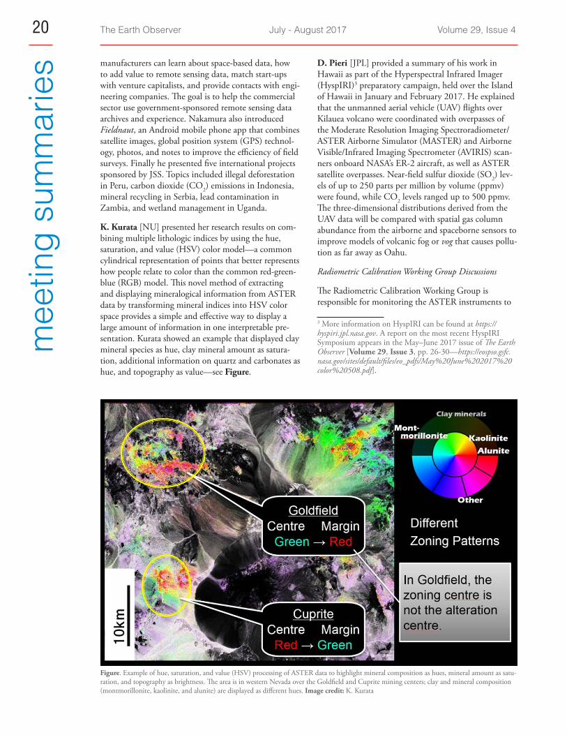
The Earth Observer July - August 2017 Volume 29, Issue 420m

eetin

g su

mm

arie

s manufacturers can learn about space-based data, how to add value to remote sensing data, match start-ups with venture capitalists, and provide contacts with engi-neering companies. The goal is to help the commercial sector use government-sponsored remote sensing data archives and experience. Nakamura also introduced Fieldnaut, an Android mobile phone app that combines satellite images, global position system (GPS) technol-ogy, photos, and notes to improve the efficiency of field surveys. Finally he presented five international projects sponsored by JSS. Topics included illegal deforestation in Peru, carbon dioxide (CO2) emissions in Indonesia, mineral recycling in Serbia, lead contamination in Zambia, and wetland management in Uganda.

K. Kurata [NU] presented her research results on com-bining multiple lithologic indices by using the hue, saturation, and value (HSV) color model—a common cylindrical representation of points that better represents how people relate to color than the common red-green-blue (RGB) model. This novel method of extracting and displaying mineralogical information from ASTER data by transforming mineral indices into HSV color space provides a simple and effective way to display a large amount of information in one interpretable pre-sentation. Kurata showed an example that displayed clay mineral species as hue, clay mineral amount as satura-tion, additional information on quartz and carbonates as hue, and topography as value—see Figure.

D. Pieri [JPL] provided a summary of his work in Hawaii as part of the Hyperspectral Infrared Imager (HyspIRI)3 preparatory campaign, held over the Island of Hawaii in January and February 2017. He explained that the unmanned aerial vehicle (UAV) flights over Kilauea volcano were coordinated with overpasses of the Moderate Resolution Imaging Spectroradiometer/ASTER Airborne Simulator (MASTER) and Airborne Visible/Infrared Imaging Spectrometer (AVIRIS) scan-ners onboard NASA’s ER-2 aircraft, as well as ASTER satellite overpasses. Near-field sulfur dioxide (SO2) lev-els of up to 250 parts per million by volume (ppmv) were found, while CO2 levels ranged up to 500 ppmv. The three-dimensional distributions derived from the UAV data will be compared with spatial gas column abundance from the airborne and spaceborne sensors to improve models of volcanic fog or vog that causes pollu-tion as far away as Oahu.

Radiometric Calibration Working Group Discussions

The Radiometric Calibration Working Group is responsible for monitoring the ASTER instruments to

3 More information on HyspIRI can be found at https://hyspiri.jpl.nasa.gov. A report on the most recent HyspIRI Symposium appears in the May–June 2017 issue of The Earth Observer [Volume 29, Issue 3, pp. 26-30—https://eospso.gsfc.nasa.gov/sites/default/files/eo_pdfs/May%20June%202017%20color%20508.pdf].

Figure. Example of hue, saturation, and value (HSV) processing of ASTER data to highlight mineral composition as hues, mineral amount as satu-ration, and topography as brightness. The area is in western Nevada over the Goldfield and Cuprite mining centers; clay and mineral composition (montmorillonite, kaolinite, and alunite) are displayed as different hues. Image credit: K. Kurata

The Earth Observer July - August 2017 Volume 29, Issue 4 21

mee

ting

sum

mar

iesunderstand and characterize their responses to scenes

being observed. The group noted that the instru-ment response is changing smoothly with time. The group also determined updated calibration coefficients to maintain calibration of the data. To monitor the instruments’ performance, the team uses data from the onboard calibration lamps for the VNIR channels and onboard blackbody for the TIR, combined with in situ field validation campaigns.

F. Sakuma [JSS] reported on the onboard calibration data using two standard lamps. These lamps were cali-brated against NIST standards before launch. Their behavior since launch has been monitored with therm-istors with well-defined characteristics. As a result, the data are within 1% of the radiometric calibration curves that are used to calibrate the VNIR data. Long-term calibration of the TIR bands, using the onboard black-body and in situ field validation results, continues to be within the threshold of the radiometric calibration curves. In February 2017 the Radiometric Calibration Coefficients (RCC) were updated to reflect small changes in detector responses.

J. Czapla-Myers [UA], H. Yamamoto [AIST], H. Tanooka [IU], S. Kato [AIST], and M. Abrams [JPL] presented field campaign results. In situ validation experiments are used in conjunction with the onboard calibration lamps and blackbody to assess the instru-ment performance and to update the calibration coef-ficients. Field campaigns were conducted in the western U.S. at large playas (the Railroad Valley, Alkali Lake, and Ivanpah playa, all in Nevada) and on Kasumigaura Lake in Japan. In the U.S., data from instrumented, autoreporting validation sites (Lake Tahoe and Salton Sea) supplemented the field campaign results. Despite the fact that the previous nine months had been cloud-ier than average, sufficient data were acquired to con-firm that the instrument VNIR and TIR responses were well understood and characterized.

This session also included an in-depth discussion of the upcoming Lunar Deep Space Calibration maneu-ver for Terra, which is currently scheduled for August 5, 2017. The Flight Operations Team plans to have Terra perform a 360° pitch maneuver to look at deep space and the moon—repeating an experiment con-ducted in 2003—to obtain accurate performance and response characteristics for the ASTER detectors. In addition, MODIS and the Multi-angle Imaging Spectroradiometer (MISR) will obtain similar calibra-tion data. The Flight Operations Team, working with each instrument team, has spent the last 12 months scripting and practicing the maneuver.

T. Kouyama [AIST], S. Kato [AIST] and F. Sakuma [JSS] described several aspects of the experiment, pro-viding a recap of the 2003 maneuver and the results obtained. They explained that the lunar data obtained

in 2003 were used to help calibrate ASTER data and to reveal minor artifacts in the imaging systems. They explained that the 2017 date selected for the maneuver is the best match for the phase angle of the moon rela-tive to Terra such as occurred in 2003. A contingency date in November 2017 has been selected in case the maneuver is waved off (e.g., in the event a debris avoid-ance maneuver is required).

Level 1-DEM Working Group Discussions

The DEM Working Group evaluated improvements to Global Digital Elevation Model, Version 3, (GDEM3), planned for release in July-August 2017 as an ASTER standard product, replacing the current Version 2.

H. Fujisada [SILC] and R. Crippen [JPL] presented similar methods to address the remaining artifacts in GDEM3. They agreed to work together to produce a combined, cleaned-up GDEM3 for release later this summer. This release will have the minimum number of artifacts of any GDEM version, as each successive ver-sion is improved from the previous version. GDEM3 will be the final GDEM produced and released by the ASTER project.

H. Fujisada [SILC] discussed corrections and improve-ments he had made to GDEM3, in version 3.1. Describing his four-step process, he stated that the first step was to replace bad GDEM values with those obtained from Shuttle Radar Topography Mission (SRTM) V3, Alaska DEM, and Canadian Digital Elevation Data (CDED). Fujisada explained that in cases where none of the data sources identified in step one were available, he used GMTED2010 7.5 arc-sec-ond data.4 Further, he explained that where none of the datasets were available, he used interpolation. Step four was to correct a few errors of land adjacent to shoreline, with SRTM V3 data. Volcanic basalt was incorrectly identified as ocean on Norfolk Island, for example. Fujisada then showed examples where these errors were fixed using this four-step process.

R. Crippen [JPL] presented his work to remove arti-facts in GDEM3, mainly the result of cloud edges that were not removed in the compilation procedure. His method was to: mask the errors in GDEM3; mask errors in GDEM2; fill GDEM3 voids with either GDEM2 or SRTM data; and then fill any remaining voids by interpolation. Additionally, Crippen planned to fix tile edge mismatches (unknown source of error), fix errors of places with negative elevations, replace bad Canadian DEM values, fix coastal issues, and increase SRTM fill resolution using newly-reprocessed SRTM

4 The 2010 Global Multi-resolution Terrain Elevation Data (GMTED2010) is an elevation dataset from the U.S. Geological Survey and National Geospatial-Intelligence Agency. The data are provided at 30-, 15-, and 7.5-arc-second spatial resolutions.

The Earth Observer July - August 2017 Volume 29, Issue 422m

eetin

g su

mm

arie

s data. He showed examples to illustrate the effectiveness of his methods.

Temperature-Emissivity Separation Working Group Discussions

The Temperature-Emissivity Separation Working Group is responsible for monitoring and maintain-ing the algorithms to produce the calibrated tempera-ture and emissivity ASTER products from the Level 1 TIR data. The group monitors the acquisition program that obtains global coverage of Earth’s entire land sur-face. A time-series is obtained by repeating the acquisi-tion scheduling on a regular—i.e., several-year—basis. Repeat coverage allows monitoring of changes to the land surface from natural or anthropogenic causes, such as desertification.

Y. Takahashi’s work on estimating oil thickness over water using ASTER thermal data was presented by co-author H. Tonooka [IU]. They analyzed data from the Gulf of Mexico’s New Horizon spill in 2010 and the Bunga Kelana 3 spill off Singapore in 2010. Their tech-nique is based on an oil-film radiation model described by Matsui et al. in 1974 that related the TIR values in different wavelengths, to the thickness of an oil film.5 For the New Horizon spill, results from ASTER and MODIS gave consistent and similar results; however, oil thickness near the leak point was smaller than its surroundings because the model was developed for oil films, not for thick oil layers. The second case they ana-lyzed, the Bunga Kelana spill, produced results that were consistent with reported amounts derived from in-water measurements.

H. Tonooka [IU] summarized the progress of the nighttime TIR data acquisition program, the goal for which is to obtain global nighttime TIR coverage on a recurring basis, which would be similar to the coverage for the daytime global mapping activity. The present acquisition program has been operating for the past 23 months. During the near-two-year acquisition of data, about 80% of the targeted areas had been observed at least once under clear sky conditions. Because there are few areas that had not been imaged, the group recom-mended restarting the nighttime global mapping this month (as if no data had yet been acquired).

Operations and Mission Planning Working Group Discussions

The Operations and Mission Planning Working Group oversees all scheduling of ASTER instruments. Because ASTER acquires data only on demand, a complex scheduling algorithm has been developed to assem-ble daily schedules for which scenes will be acquired.

5 M. Matsui, Watanabe, K., Yoshida, K., et al., 1974, Hydrocarbon Components of Floating Oil Pollutants of Sea-water, Bull. Japanese Soc. Of Scientific Fisheries, 40, 111-116.

Various mapping programs take place simultaneously, such as the global mapping program that operates in the background when no higher-priority acquisitions are scheduled.

M. Fujita [JSS] presented summaries and status updates on all of the ongoing acquisition programs. The Global Mapping-7 program has successfully acquired about 44% of the programmed scenes with 20% or less cloud cover; the group recommended continuing it for at least one more year. The cur-rently running Nighttime TIR Global Mapping was to be suspended, and the next mapping program was to begin, based on recommendations from the Temperature-Emissivity Separation Working Group. The Underserved Area program (an effort to acquire images over persistently cloudy areas) will be contin-ued for at least one more year. The Glacier Monitoring Program will be restarted in the next few months based on recommendation from the Global Land Ice Measurements from Space (GLIMS) project. The Volcano Monitoring Program (which provides frequent day and night coverage of 1500 active volcanoes) will continue for the next few years. The Remote Island Program (which obtains single scenes over isolated mid-ocean targets) will continue. Urgent observations (e.g., field campaigns, volcano monitoring, and natural hazards) were summarized, and the reasons for the 2% failures of the urgent and field campaign requests (3 of 143) were examined individually. The failures occurred because of requests received after the allowed schedul-ing window had closed.

T. Tachikawa [JSS] presented a summary of the cloud avoidance algorithm performance. By using cloud predic-tions, data acquisition efficiency increased about 10%.

Closing Plenary Session

The chairpersons of each of the working groups pre-sented summaries of discussions and presentations for each of their sessions. Further discussion of the infor-mation presented during the sessions by the entire team was encouraged. The Terra platform and the ASTER instrument are performing normally, with no change since the preceding 2016 team meeting. Continuing discussions about the August 2017 Lunar and Deep Space Calibration maneuver verified that plans were acceptable and the maneuver would be carried out as scheduled. The GDEM Version 3 will be released in summer 2017, pending final correction of the few remaining artifacts. The next meeting will be held June 4-6, 2018, at the same venue in Tokyo.

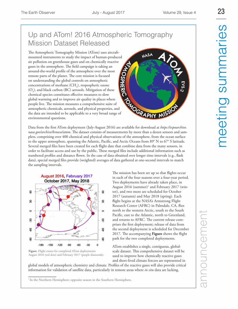
The Earth ObserverThe Earth Observer July - August 2017July - August 2017 Volume 29, Issue 4Volume 29, Issue 4 23

mee

ting

sum

mar

ies

23

Up and ATom! 2016 Atmospheric Tomography Mission Dataset Released The Atmospheric Tomography Mission (ATom) uses aircraft-mounted instruments to study the impact of human-produced air pollution on greenhouse gases and on chemically reactive gases in the atmosphere. The field campaign is taking an around-the-world profile of the atmosphere over the most remote parts of the planet. The core mission is focused on understanding the global controls on atmospheric concentrations of methane (CH4), tropospheric ozone (O3), and black carbon (BC) aerosols. Mitigation of these chemical species constitutes effective measures to slow global warming and to improve air quality in places where people live. The mission measures a comprehensive suite of atmospheric chemicals, aerosols, and physical properties, and the data are intended to be applicable to a very broad range of environmental questions.

Data from the first ATom deployment (July-August 2016) are available for download at https://espoarchive.nasa.gov/archive/browse/atom. The dataset consists of measurements by more than a dozen sensors and sam-plers, comprising over 400 chemical and physical observations of the atmosphere, from the ocean surface to the upper atmosphere, spanning the Atlantic, Pacific, and Arctic Oceans from 89° N to 67° S latitude. Several merged files have been created for each flight date that combine data from the many sensors, in order to facilitate access and use by the public. These merged files include additional information such as numbered profiles and distance flown. In the case of data obtained over longer time intervals (e.g., flask data), special merged files provide (weighted) averages of data gathered at one-second intervals to match the sampling intervals.

The mission has been set up so that flights occur in each of the four seasons over a four-year period. Two deployments have already taken place, in August 2016 (summer)1 and February 2017 (win-ter), and two more are scheduled for October 2017 (autumn) and May 2018 (spring). Each flight begins at the NASA’s Armstrong Flight Research Center (AFRC) in Palmdale, CA, flies north to the western Arctic, south to the South Pacific, east to the Atlantic, north to Greenland, and returns to AFRC. The current release com-prises the first deployment; release of data from the second deployment is scheduled for December 2017. The accompanying Figure shows the flight path for the two completed deployments.

ATom establishes a single, contiguous, global-scale dataset. This comprehensive dataset will be used to improve how chemically reactive gases and short-lived climate forcers are represented in

global models of atmospheric chemistry and climate. Profiles of the reactive gases will also provide critical information for validation of satellite data, particularly in remote areas where in situ data are lacking.

1 In the Northern Hemisphere; opposite season in the Southern Hemisphere.

Figure. Flight routes for completed ATom deployments: August 2016 (red dots) and February 2017 (purple diamonds).

anno

unce

men

t

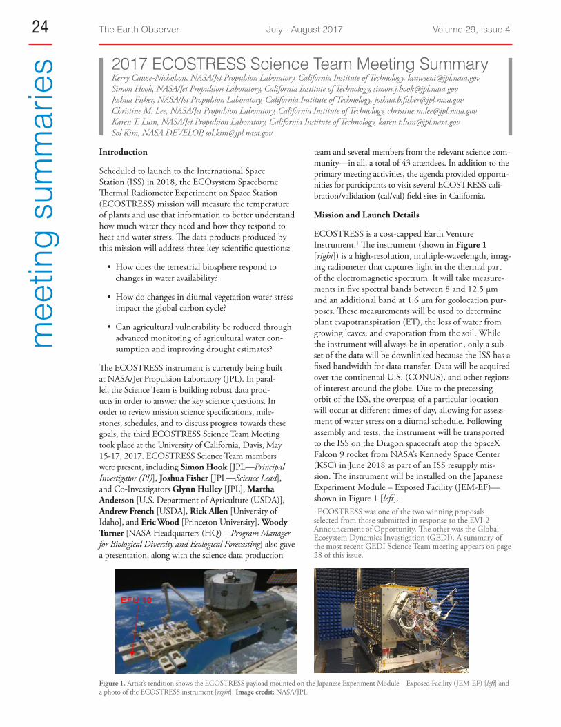
The Earth Observer July - August 2017 Volume 29, Issue 424m

eetin

g su

mm

arie

s

team and several members from the relevant science com-munity—in all, a total of 43 attendees. In addition to the primary meeting activities, the agenda provided opportu-nities for participants to visit several ECOSTRESS cali-bration/validation (cal/val) field sites in California.

Mission and Launch Details

ECOSTRESS is a cost-capped Earth Venture Instrument.1 The instrument (shown in Figure 1 [right]) is a high-resolution, multiple-wavelength, imag-ing radiometer that captures light in the thermal part of the electromagnetic spectrum. It will take measure-ments in five spectral bands between 8 and 12.5 µm and an additional band at 1.6 µm for geolocation pur-poses. These measurements will be used to determine plant evapotranspiration (ET), the loss of water from growing leaves, and evaporation from the soil. While the instrument will always be in operation, only a sub-set of the data will be downlinked because the ISS has a fixed bandwidth for data transfer. Data will be acquired over the continental U.S. (CONUS), and other regions of interest around the globe. Due to the precessing orbit of the ISS, the overpass of a particular location will occur at different times of day, allowing for assess-ment of water stress on a diurnal schedule. Following assembly and tests, the instrument will be transported to the ISS on the Dragon spacecraft atop the SpaceX Falcon 9 rocket from NASA’s Kennedy Space Center (KSC) in June 2018 as part of an ISS resupply mis-sion. The instrument will be installed on the Japanese Experiment Module – Exposed Facility (JEM-EF)—shown in Figure 1 [left]. 1 ECOSTRESS was one of the two winning proposals selected from those submitted in response to the EVI-2 Announcement of Opportunity. The other was the Global Ecosystem Dynamics Investigation (GEDI). A summary of the most recent GEDI Science Team meeting appears on page 28 of this issue.

2017 ECOSTRESS Science Team Meeting Summary Kerry Cawse-Nicholson, NASA/Jet Propulsion Laboratory, California Institute of Technology, kcawseni@jpl.nasa.gov Simon Hook, NASA/Jet Propulsion Laboratory, California Institute of Technology, simon.j.hook@jpl.nasa.govJoshua Fisher, NASA/Jet Propulsion Laboratory, California Institute of Technology, joshua.b.fisher@jpl.nasa.gov Christine M. Lee, NASA/Jet Propulsion Laboratory, California Institute of Technology, christine.m.lee@jpl.nasa.gov Karen T. Lum, NASA/Jet Propulsion Laboratory, California Institute of Technology, karen.t.lum@jpl.nasa.gov Sol Kim, NASA DEVELOP, sol.kim@jpl.nasa.gov

Introduction

Scheduled to launch to the International Space Station (ISS) in 2018, the ECOsystem Spaceborne Thermal Radiometer Experiment on Space Station (ECOSTRESS) mission will measure the temperature of plants and use that information to better understand how much water they need and how they respond to heat and water stress. The data products produced by this mission will address three key scientific questions:

• How does the terrestrial biosphere respond to changes in water availability?

• How do changes in diurnal vegetation water stress impact the global carbon cycle?

• Can agricultural vulnerability be reduced through advanced monitoring of agricultural water con-sumption and improving drought estimates?

The ECOSTRESS instrument is currently being built at NASA/Jet Propulsion Laboratory (JPL). In paral-lel, the Science Team is building robust data prod-ucts in order to answer the key science questions. In order to review mission science specifications, mile-stones, schedules, and to discuss progress towards these goals, the third ECOSTRESS Science Team Meeting took place at the University of California, Davis, May 15-17, 2017. ECOSTRESS Science Team members were present, including Simon Hook [JPL—Principal Investigator (PI)], Joshua Fisher [JPL—Science Lead], and Co-Investigators Glynn Hulley [JPL], Martha Anderson [U.S. Department of Agriculture (USDA)], Andrew French [USDA], Rick Allen [University of Idaho], and Eric Wood [Princeton University]. Woody Turner [NASA Headquarters (HQ)—Program Manager for Biological Diversity and Ecological Forecasting] also gave a presentation, along with the science data production

Figure 1. Artist’s rendition shows the ECOSTRESS payload mounted on the Japanese Experiment Module – E xposed Facility (JEM-EF) [left] and a photo of the ECOSTRESS instrument [right]. Image credit: NASA/JPL

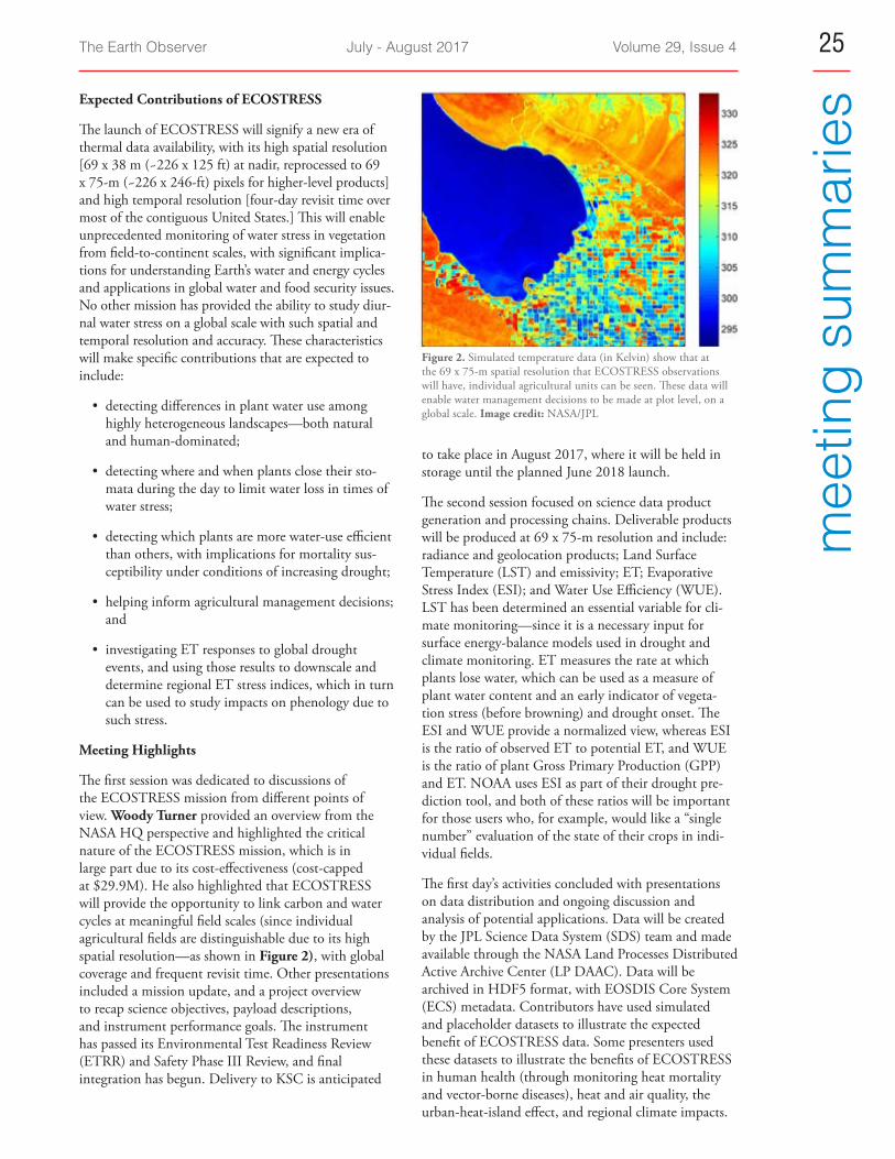
The Earth Observer July - August 2017 Volume 29, Issue 4 25

mee

ting

sum

mar

iesExpected Contributions of ECOSTRESS

The launch of ECOSTRESS will signify a new era of thermal data availability, with its high spatial resolution [69 x 38 m (~226 x 125 ft) at nadir, reprocessed to 69 x 75-m (~226 x 246-ft) pixels for higher-level products] and high temporal resolution [four-day revisit time over most of the contiguous United States.] This will enable unprecedented monitoring of water stress in vegetation from field-to-continent scales, with significant implica-tions for understanding Earth’s water and energy cycles and applications in global water and food security issues. No other mission has provided the ability to study diur-nal water stress on a global scale with such spatial and temporal resolution and accuracy. These characteristics will make specific contributions that are expected to include:

• detecting differences in plant water use among highly heterogeneous landscapes—both natural and human-dominated;

• detecting where and when plants close their sto-mata during the day to limit water loss in times of water stress;

• detecting which plants are more water-use efficient than others, with implications for mortality sus-ceptibility under conditions of increasing drought;

• helping inform agricultural management decisions; and

• investigating ET responses to global drought events, and using those results to downscale and determine regional ET stress indices, which in turn can be used to study impacts on phenology due to such stress.

Meeting Highlights

The first session was dedicated to discussions of the ECOSTRESS mission from different points of view. Woody Turner provided an overview from the NASA HQ perspective and highlighted the critical nature of the ECOSTRESS mission, which is in large part due to its cost-effectiveness (cost-capped at $29.9M). He also highlighted that ECOSTRESS will provide the opportunity to link carbon and water cycles at meaningful field scales (since individual agricultural fields are distinguishable due to its high spatial resolution—as shown in Figure 2), with global coverage and frequent revisit time. Other presentations included a mission update, and a project overview to recap science objectives, payload descriptions, and instrument performance goals. The instrument has passed its Environmental Test Readiness Review (ETRR) and Safety Phase III Review, and final integration has begun. Delivery to KSC is anticipated

to take place in August 2017, where it will be held in storage until the planned June 2018 launch.

The second session focused on science data product generation and processing chains. Deliverable products will be produced at 69 x 75-m resolution and include: radiance and geolocation products; Land Surface Temperature (LST) and emissivity; ET; Evaporative Stress Index (ESI); and Water Use Efficiency (WUE). LST has been determined an essential variable for cli-mate monitoring—since it is a necessary input for surface energy-balance models used in drought and climate monitoring. ET measures the rate at which plants lose water, which can be used as a measure of plant water content and an early indicator of vegeta-tion stress (before browning) and drought onset. The ESI and WUE provide a normalized view, whereas ESI is the ratio of observed ET to potential ET, and WUE is the ratio of plant Gross Primary Production (GPP) and ET. NOAA uses ESI as part of their drought pre-diction tool, and both of these ratios will be important for those users who, for example, would like a “single number” evaluation of the state of their crops in indi-vidual fields.

The first day’s activities concluded with presentations on data distribution and ongoing discussion and analysis of potential applications. Data will be created by the JPL Science Data System (SDS) team and made available through the NASA Land Processes Distributed Active Archive Center (LP DAAC). Data will be archived in HDF5 format, with EOSDIS Core System (ECS) metadata. Contributors have used simulated and placeholder datasets to illustrate the expected benefit of ECOSTRESS data. Some presenters used these datasets to illustrate the benefits of ECOSTRESS in human health (through monitoring heat mortality and vector-borne diseases), heat and air quality, the urban-heat-island effect, and regional climate impacts.

Figure 2. Simulated temperature data (in Kelvin) show that at the 69 x 75-m spatial resolution that ECOSTRESS observations will have, individual agricultural units can be seen. These data will enable water management decisions to be made at plot level, on a global scale. Image credit: NASA/JPL

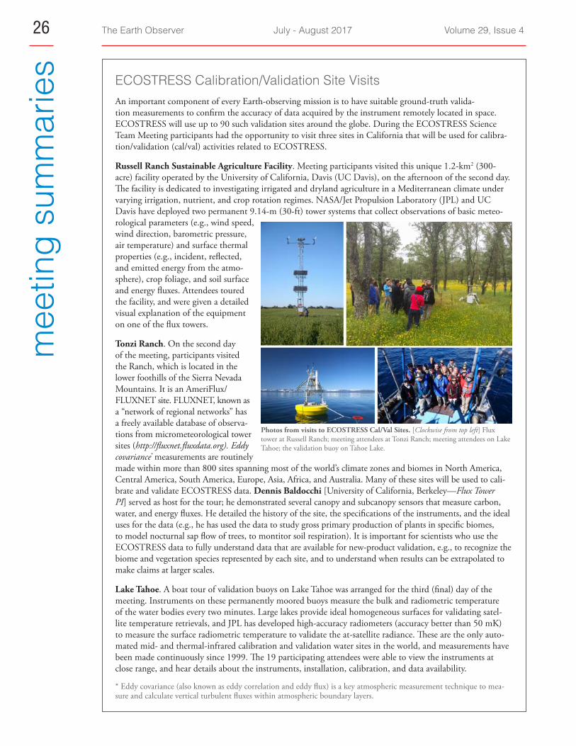
The Earth Observer July - August 2017 Volume 29, Issue 426m

eetin

g su

mm

arie

s ECOSTRESS Calibration/Validation Site VisitsAn important component of every Earth-observing mission is to have suitable ground-truth valida-tion measurements to confirm the accuracy of data acquired by the instrument remotely located in space. ECOSTRESS will use up to 90 such validation sites around the globe. During the ECOSTRESS Science Team Meeting participants had the opportunity to visit three sites in California that will be used for calibra-tion/validation (cal/val) activities related to ECOSTRESS.

Russell Ranch Sustainable Agriculture Facility. Meeting participants visited this unique 1.2-km2 (300-acre) facility operated by the University of California, Davis (UC Davis), on the afternoon of the second day. The facility is dedicated to investigating irrigated and dryland agriculture in a Mediterranean climate under varying irrigation, nutrient, and crop rotation regimes. NASA/Jet Propulsion Laboratory (JPL) and UC Davis have deployed two permanent 9.14-m (30-ft) tower systems that collect observations of basic meteo-rological parameters (e.g., wind speed, wind direction, barometric pressure, air temperature) and surface thermal properties (e.g., incident, reflected, and emitted energy from the atmo-sphere), crop foliage, and soil surface and energy fluxes. Attendees toured the facility, and were given a detailed visual explanation of the equipment on one of the flux towers.

Tonzi Ranch. On the second day of the meeting, participants visited the Ranch, which is located in the lower foothills of the Sierra Nevada Mountains. It is an AmeriFlux/FLUXNET site. FLUXNET, known as a “network of regional networks” has a freely available database of observa-tions from micrometeorological tower sites (http://fluxnet.fluxdata.org). Eddy covariance* measurements are routinely made within more than 800 sites spanning most of the world’s climate zones and biomes in North America, Central America, South America, Europe, Asia, Africa, and Australia. Many of these sites will be used to cali-brate and validate ECOSTRESS data. Dennis Baldocchi [University of California, Berkeley—Flux Tower PI] served as host for the tour; he demonstrated several canopy and subcanopy sensors that measure carbon, water, and energy fluxes. He detailed the history of the site, the specifications of the instruments, and the ideal uses for the data (e.g., he has used the data to study gross primary production of plants in specific biomes, to model nocturnal sap flow of trees, to montitor soil respiration). It is important for scientists who use the ECOSTRESS data to fully understand data that are available for new-product validation, e.g., to recognize the biome and vegetation species represented by each site, and to understand when results can be extrapolated to make claims at larger scales.

Lake Tahoe. A boat tour of validation buoys on Lake Tahoe was arranged for the third (final) day of the meeting. Instruments on these permanently moored buoys measure the bulk and radiometric temperature of the water bodies every two minutes. Large lakes provide ideal homogeneous surfaces for validating satel-lite temperature retrievals, and JPL has developed high-accuracy radiometers (accuracy better than 50 mK) to measure the surface radiometric temperature to validate the at-satellite radiance. These are the only auto-mated mid- and thermal-infrared calibration and validation water sites in the world, and measurements have been made continuously since 1999. The 19 participating attendees were able to view the instruments at close range, and hear details about the instruments, installation, calibration, and data availability.

* Eddy covariance (also known as eddy correlation and eddy flux) is a key atmospheric measurement technique to mea-sure and calculate vertical turbulent fluxes within atmospheric boundary layers.

Photos from visits to ECOSTRESS Cal/Val Sites. [Clockwise from top left] Flux tower at Russell Ranch; meeting attendees at Tonzi Ranch; meeting attendees on Lake Tahoe; the validation buoy on Tahoe Lake.

The Earth Observer July - August 2017 Volume 29, Issue 4 27

mee

ting

sum

mar

iesOther scientists showed the role of satellite ET data in

scheduling irrigation, predicting seasonal water use, and as input to other agricultural water management techniques at various sites in North and Central America. In such applications the field-level spatial scale of ECOSTRESS will provide an immediate benefit to precision agriculture. From these presentations, it is clear that the science community is preparing for ECOSTRESS data.

The primary focus of the second day was to discuss ECOSTRESS calibration and validation (cal/val) techniques and data simulations, and to allow meet-ing participants to hear about and visit several cal/val sites in California. Approximately 30 attendees visited both the Russell Ranch Sustainable Agriculture Facility and Tonzi Ranch sites. The third and final day of the meeting was used a visit to the Lake Tahoe site. To

learn more about these “field trips,” see ECOSTRESS Calibration/Validation Site Visits on the previous page.

Conclusion

The third ECOSTRESS Science Team Meeting pro-vided an opportunity to update the Team and com-munity members on progress towards meeting ECOSTRESS science goals and objectives. It also pro-vided an opportunity for community input, and to initiate and foster beneficial collaborations. Additional information about ECOSTRESS is available online at http://ecostress.jpl.nasa.gov.

The research was carried out at the Jet Propulsion Laboratory, California Institute of Technology, under a contract with the National Aeronautics and Space Administration.

© 2017 California Institute of Technology. Government sponsorship acknowledged.

DSCOVR EPIC and NISTAR Level-1 Data Released The Deep Space Climate Observatory (DSCOVR) is a joint NASA-National Oceanic and Atmospheric Administration (NOAA) mission located near the Earth-sun Lagrange point L11 where it performs its primary objective of monitoring the solar wind as well as observing the Earth from sunrise to sunset with two Earth sci-ence sensors: the Earth Polychromatic Imaging Camera (EPIC) and the National Institute of Standards and Technology (NIST) Advanced Radiometer [NISTAR].  The Earth sensors measure the broadband radiative fluxes of the entire dayside of Earth (NISTAR) as well as key spectral radiative characteristics in 10 narrowband channels between 317 and 790 nm at 10-20-km spatial resolution (EPIC).  

The DSCOVR project, together with the DSCOVR Earth Sensors science team and the Atmospheric Science Data Center (ASDC) at NASA’s Langley Research Center, announce the release of both Earth sensors’ Level-1 data.  The release of Level-1 EPIC data provides 10 channel spectral radiances in counts per second units.  The calibration factors that convert counts per second into reflectance are also provided.  The released datasets have (Level-1A) instrument calibrations, flat-fielding, stray-light correction and (Level-1B) geolocation applied.  

The release of Level-1 NISTAR data provides irradiance meaurements in three broadband ranges from three active cavity radiometers. The total channel measures both solar-reflected and Earth-thermal radiation, the shortwave channel extracts the solar reflected irradiance, and the third channel is limited to the near infrared solar reflected signal. The fourth detector is a high signal-to-noise photodiode spanning ultraviolet (UV), vis-ible, and near-infrared (NIR) frequencies. Absolute calibration parameters are provided.

The released data are available from June 2015 through the current day via the ASDC Earthdata Search at https://earthdata.nasa.gov/search?q=DSCOVR. Color imagery can be seen at http://epic.gsfc.nasa.gov.  New Level 1 data will be released approximately 24-36 hours after observations.  Information about data formats can be found in the EPIC Data Format Control Book at https://eosweb.larc.nasa.gov/project/dscovr/EPIC_Data_Format_Control_Book_2016-07-01.pdf and in the NISTAR Data Format Control Book at https://eosweb.larc.nasa.gov/proj-ect/dscovr/NISTAR_Data_Format_Control_Book_2016-07-01.pdf.

NOAA releases data from the space weather instruments onboard DSCOVR. The data, as well as space weather forecasts with a 30-45 minute lead-time, are available via the Space Weather Prediction Center at http://www.swpc.noaa.gov.

1 A Lagrange point is a point in space where the combined gravitational forces of two large bodies equal the centrifugal force felt by a much smaller third body. L1 is the Lagrange point between the Earth and the sun. The DSCOVR spacecraft is essentially “parked” at the L1 posi-tion (~1 million miles from Earth) and makes continuous observations of both the sun and Earth. anno

unce

men

t

The Earth Observer July - August 2017 Volume 29, Issue 428m

eetin

g su

mm

arie

s

Scott Luthcke [GSFC] provided an update on the GEDI data management plan, which will soon need input from the GEDI SDT members. Once GEDI is operational, the Science Operations Center (SOC) will be periodically provided with updated target pri-ority maps and digitizer settings.3 Plans to implement the GEDI science data system to facilitate data stor-age, processing, and access—both within GSFC and at UMD—are also under development.

Data Products Discussion

The GEDI ATBDs4 provide both the physical the-ory as well as the mathematical procedures and pos-sible assumptions being applied to convert the energy received by the instrument to geophysical quanti-ties. Such a document has been drafted for each of the Level-1 to -4 data products—listed in Table. The SOC will use these ATBDs to implement data process-ing algorithms. Several of the product Levels have an A and a B product; for implementation, the B product is always dependent on its A product. The first versions of these documents were completed prior to CDR, fol-lowed by internal reviews, subsequent revisions, and submission for external review.

Michele Hofton [UMD/GSFC] is leading develop-ment of the Level-1A and -2A data products. These products are outlined in a single ATBD, as they heavily depend on each other and are highly similar to algo-rithms in use for the Land, Vegetation, and Ice Sensor (LVIS) waveform processing chain. The LVIS—the airborne predecessor of GEDI—has been operational since 1999 and has similar instrument and data char-acteristics as the GEDI. (Bryan Blair and Michele Hofton have been involved with LVIS from the begin-ning and have developed and improved the instrument and the data processing algorithms thoroughly, result-ing in high expertise and great preparation for GEDI.)

Scott Luthcke leads the Level-1B product development team. He summarized the pointing and positioning sys-tem needed to calibrate and geolocate the waveforms.

3 During the mission, parameters of the GEDI sensor can be tweaked in the Science Operation Center—for example to change laser pointing (enabling full coverage of as-yet un-sampled areas) or switch to a different beam-dithering mode over certain targets. 4 Historicaly, ATBDs have been created for many of the data products for Earth Observing System instruments. A partial list of ATBDs can be found at https://eospso.gsfc.nasa.gov/con-tent/algorithm-theoretical-basis-documents. Click on the instru-ment acronyms to see expanded lists of data product ATBDs.

Summary of the Third GEDI Science Definition Team Meeting Suzanne Marselis, University of Maryland, College Park, marselis@umd.edu John Armston, University of Maryland, College Park, armston@umd.edu J. Bryan Blair, NASA’s Goddard Space Flight Center, james.b.blair@nasa.gov Ralph Dubayah, University of Maryland, College Park, dubayah@umd.edu

The third Global Ecosystem Dynamics Investigation (GEDI) Science Definition Team (SDT) meeting took place April 4-6, 2017, at the National Socio-Environmental Synthesis Center (SESYNC) in Annapolis, MD. Twenty-seven SDT members, collabo-rators, and associates attended the meeting. The main objectives of the meeting were to discuss the GEDI data product algorithms and drafts of the Algorithm Theoretical Basis Documents (ATBDs) and to review and update the GEDI calibration/validation (cal/val) plans.1

Mission Status

Ralph Dubayah [University of Maryland, College Park (UMD)—GEDI Principal Investigator] convened the meeting and commenced with a short overview of the current mission status. GEDI remains on schedule for launch in December 2018.

Jim Pontius [NASA’s Goddard Space Flight Center (GSFC)—GEDI Project Manager] highlighted GEDI’s successful completion of the Critical Design Review (CDR) in February 2017 and affirmed that the mis-sion continues to meet all technical, cost, and schedule milestones as well as its Level-1 Science Requirements. Engineering model hardware fabrication and key inter-face testing are wrapping up, flight-model fabrication is fully underway, integration and test facilities are ready, and the Ground System and Mission Operations Center are nearly complete.

Bryan Blair [GSFC—GEDI Deputy Principal Investigator and Instrument Scientist] brought positive news on the instrument development status, highlighting that expected sensor performance remains solid with good margins. He detailed that the proposed solution to an issue causing laser side-lobes was successful and that the laser now exhibits Gaussian spatial beam quality.2 One current focus for the team is to simulate the performance of the GEDI global positioning system (GPS) in its planned location on the International Space Station (ISS) to ensure the desired geo-location accuracy of ~7 m, or ~23 ft (equal to one standard deviation).

1 More information on the GEDI mission and the previous SDT meeting can be found in the November-December 2016 issue of The Earth Observer [Volume 28, Issue 6, pp. 31-36—https://eospso.nasa.gov/sites/default/files/eo_pdfs/Nov-Dec%202016%20color%20508.pdf]. 2 GEDI’s laser footprint energy follows a two-dimensional Gaussian distribution, exhibiting stronger power in the cen-ter and fading towards the edges. The nominal footprint size (22 m) indicates the diameter, within which, which 86% of the energy is contained.

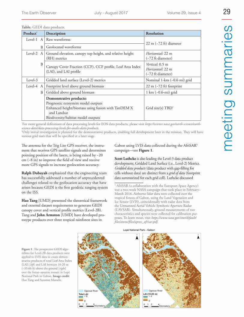
The Earth Observer July - August 2017 Volume 29, Issue 4 29

mee

ting

sum

mar

iesTable. GEDI data products.

Product* Description Resolution

Level-1 A Raw waveforms22 m (~72 ft) diameter

B Geolocated waveforms

Level-2 A Ground elevation, canopy top height, and relative height Horizontal: 22 m (RH) metrics (~72 ft diameter)

B Vertical: 0.5 m Canopy Cover Fraction (CCF), CCF profile, Leaf Area Index Horizontal: 22 m (LAI), and LAI profile (~72 ft diameter) Level-3 Gridded land surface (Level-2) metrics Nominal 1-km (~0.6 mi) grid

Level-4 A Footprint level above ground biomass 22 m (~72 ft) footprint

B Gridded above ground biomass 1 km (~0.6-mi) gridDemonstrative products: Prognostic ecosystem model outputs Enhanced height/biomass using fusion with TanDEM X Grid size(s) TBD†

and Landsat Biodiversity/habitat model outputs

*For more general definitions of data processing levels for EOS data products, please visit https://science.nasa.gov/earth-science/earth-science-data/data-processing-levels-for-eosdis-data-products. †Only initial investigation is planned for the demonstrative products, enabling full development later in the mission. They will have various grid sizes that will be specified at a later stage.

The antenna for the Trig Lite GPS receiver, the instru-ment that receives GPS satellite signals and determines pointing position of the lasers, is being raised by ~20 cm (~8 in) to improve the field of view and receive more GPS signals to increase geolocation accuracy.

Ralph Dubayah emphasized that the engineering team has successfully addressed a number of unprecedented challenges related to the geolocation accuracy that have arisen because GEDI is the first geodetic ranging system on the ISS.

Hao Tang [UMD] presented the theoretical framework and external dataset requirements to generate GEDI canopy cover and vertical profile metrics (Level-2B). Tang and John Armston [UMD] have developed pro-totype products over three tropical rainforest sites in

Gabon using LVIS data collected during the AfriSAR5 campaign—see Figure 1.

Scott Luthcke is also leading the Level-3 data product development, Gridded Land Surface (i.e., Level-2) Metrics. Gridded data products (data product with gap-filling for cells without data) are distinct from a grid of data (footprint data summarized for each grid cell). Luthcke discussed

5 AfriSAR (a collaboration with the European Space Agency) was a two-week NASA campaign that took place in February–March 2016. Airborne lidar data were collected over the tropical forests of Gabon, using the Land Vegetation and Ice Sensor (LVIS), coincidentally with radar data from the Unmanned Aerial Vehicle Synthetic Aperture Radar (UAVSAR). Simultaneously, ground measurements of tree characteristics and species were collected for calibration pur-poses. To learn more, visit https://www.nasa.gov/sites/default/files/atoms/files/xpress_afrisar.pdf.

Figure 1. The prospective GEDI algo-rithms for Level-2B data products were applied to LVIS data to create demon-strative products of total Leaf Area Index (LAI) [left] and LAI between 10-20 m (~33-66 ft) above the ground [right] over the forest–savanna mosaic in Lopé National Park in Gabon. Image credit: Hao Tang and Suzanne Marselis

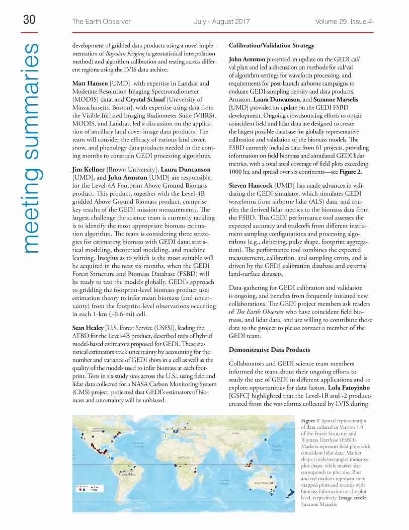
The Earth Observer July - August 2017 Volume 29, Issue 430m

eetin

g su

mm

arie

s development of gridded data products using a novel imple-mentation of Bayesian Kriging (a geostatistical interpolation method) and algorithm calibration and testing across differ-ent regions using the LVIS data archive.

Matt Hansen [UMD], with expertise in Landsat and Moderate Resolution Imaging Spectroradiometer (MODIS) data, and Crystal Schaaf [University of Massachusetts, Boston], with expertise using data from the Visible Infrared Imaging Radiometer Suite (VIIRS), MODIS, and Landsat, led a discussion on the applica-tion of ancillary land cover image data products. The team will consider the efficacy of various land cover, snow, and phenology data products needed in the com-ing months to constrain GEDI processing algorithms.

Jim Kellner [Brown University], Laura Duncanson [UMD], and John Armston [UMD] are responsible for the Level-4A Footprint Above Ground Biomass product. This product, together with the Level-4B gridded Above Ground Biomass product, comprise key results of the GEDI mission measurements. The largest challenge the science team is currently tackling is to identify the most appropriate biomass estima-tion algorithm. The team is considering three strate-gies for estimating biomass with GEDI data: statis-tical modeling, theoretical modeling, and machine learning. Insights as to which is the most suitable will be acquired in the next six months, when the GEDI Forest Structure and Biomass Database (FSBD) will be ready to test the models globally. GEDI’s approach to gridding the footprint-level biomass product uses estimation theory to infer mean biomass (and uncer-tainty) from the footprint-level observations occurring in each 1-km (~0.6-mi) cell. 

Sean Healey [U.S. Forest Service (USFS)], leading the ATBD for the Level-4B product, described tests of hybrid model-based estimators proposed for GEDI. These sta-tistical estimators track uncertainty by accounting for the number and variance of GEDI shots in a cell as well as the quality of the models used to infer biomass at each foot-print. Tests in six study sites across the U.S., using field and lidar data collected for a NASA Carbon Monitoring System (CMS) project, projected that GEDI’s estimators of bio-mass and uncertainty will be unbiased.

Calibration/Validation Strategy

John Armston presented an update on the GEDI cal/val plan and led a discussion on methods for cal/val of algorithm settings for waveform processing, and requirements for post-launch airborne campaigns to evaluate GEDI sampling density and data products. Armston, Laura Duncanson, and Suzanne Marselis [UMD] provided an update on the GEDI FSBD development. Ongoing crowdsourcing efforts to obtain coincident field and lidar data are designed to create the largest possible database for globally representative calibration and validation of the biomass models. The FSBD currently includes data from 61 projects, providing information on field biomass and simulated GEDI lidar metrics, with a total areal coverage of field plots exceeding 1000 ha, and spread over six continents—see Figure 2.

Steven Hancock [UMD] has made advances in vali-dating the GEDI simulator, which simulates GEDI waveforms from airborne lidar (ALS) data, and cou-ples the derived lidar metrics to the biomass data from the FSBD. This GEDI performance tool assesses the expected accuracy and tradeoffs from different instru-ment sampling configurations and processing algo-rithms (e.g., dithering, pulse shape, footprint aggrega-tion). The performance tool combines the expected measurement, calibration, and sampling errors, and is driven by the GEDI calibration database and external land-surface datasets.

Data-gathering for GEDI calibration and validation is ongoing, and benefits from frequently initiated new collaborations. The GEDI project members ask readers of The Earth Observer who have coincident field bio-mass, and lidar data, and are willing to contribute those data to the project to please contact a member of the GEDI team.

Demonstrative Data Products

Collaborators and GEDI science team members informed the team about their ongoing efforts to study the use of GEDI in different applications and to explore opportunities for data fusion. Lola Fatoyinbo [GSFC] highlighted that the Level-1B and -2 products created from the waveforms collected by LVIS during

Figure 2. Spatial representation of data collated in Version 1.0 of the Forest Structure and Biomass Database (FSBD). Markers represent field plots with coincident lidar data. Marker shape (circle/rectangle) indicates plot shape, while marker size corresponds to plot size. Blue and red markers represent stem-mapped plots and records with biomass information at the plot level, respectively. Image credit: Suzanne Marselis

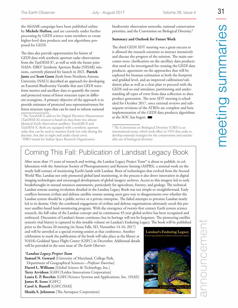
The Earth Observer July - August 2017 Volume 29, Issue 4 31

mee

ting

sum

mar

iesthe AfriSAR campaign have been published online

by Michele Hofton, and are currently under further processing by GEDI science team members to create higher-level data products and test algorithms pro-posed for GEDI.

The data also provide opportunities for fusion of GEDI data with synthetic aperture radar observations from the TanDEM-X6, as well as with the future joint NASA- ISRO7 Synthetic Aperture Radar [NISAR] mis-sions, currently planned for launch in 2021. Patrick Jantz and Scott Goetz [both from Northern Arizona University (NAU)] described an approach for developing an Essential Biodiversity Variable that uses GEDI wave-form metrics and ancillary data to quantify the extent and protected status of forest structure types in differ-ent ecoregions. A primary objective of the approach is to provide estimates of protected area representativeness for forest structure types that can be used to inform national 6 The TerraSAR-X add-on for Digital Elevation Measurement (TanDEM-X) mission is based on data from two almost identical Earth observation satellites: TerraSAR-X and TanDEM-X. Both are equipped with a synthetic aperture radar that can be used to monitor Earth not only during the daytime, but also at night and under cloud cover.7 ISRO stands for Indian Space Research Organization.

biodiversity observation networks, national conservation priorities, and the Convention on Biological Diversity.8

Summary and Outlook for Future Work

The third GEDI SDT meeting was a great success as it allowed the research scientists to interact intensively and discuss the progress of the mission. The main out-comes were: clarification on the ancillary data products that need to be investigated for creating the GEDI data products, agreement on the approaches that will be explored for biomass estimation at both the footprint and gridded level, and an improved calibration/vali-dation plan as well as a clear plan to proceed with the GEDI end-to-end simulator, partitioning and under-standing all types of error from data collection to data product generation. The next SDT meeting is sched-uled for October 2017, once external reviews and sub-sequent revisions of the ATBDs are complete and beta implementation of the GEDI data products algorithms at the SOC has begun.

8 The Convention on Biological Diversity (CBD) is an international treaty, which took effect in 1993 that seeks to develop national strategies for the conservation and sustain-able use of biological diversity.

Coming This Fall: Publication of Landsat Legacy Book After more than 15 years of research and writing, the Landsat Legacy Project Team* is about to publish, in col-laboration with the American Society of Photogrammetry and Remote Sensing (ASPRS), a seminal work on the nearly half-century of monitoring Earth’s lands with Landsat. Born of technologies that evolved from the Second World War, Landsat not only pioneered global land monitoring, in the process it also drove innovation in digital imaging technologies and encouraged development of global imagery archives. Access to this imagery led to early breakthroughs in natural resources assessments, particularly for agriculture, forestry, and geology. The technical Landsat remote sensing revolution detailed in the Landsat Legacy Book was not simple or straightforward. Early conflicts between civilian and defense satellite remote sensing users gave way to disagreements over whether the Landsat system should be a public service or a private enterprise. The failed attempts to privatize Landsat nearly led to its demise. Only the combined engagement of civilian and defense organizations ultimately saved this pio-neer satellite-based land-monitoring program. With the emergence of twenty-first century Earth system science research, the full value of the Landsat concept and its continuous 45-year global archive has been recognized and embraced. Discussion of Landsat’s future continues, but its heritage will not be forgotten. The pioneering satellite system’s vital history is captured in this notable volume on Landsat’s Enduring Legacy. The book will be published prior to the Pecora 20 meeting (in Sioux Falls, SD, November 14-16, 2017) and will be unveiled at a special evening session at that conference. Another celebration to mark the publication of the book will take place at the library at NASA’s Goddard Space Flight Center (GSFC) in December. Additional details will be provided in the next issue of The Earth Observer.

*Landsat Legacy Project Team Samuel N. Goward [University of Maryland, College Park, Department of Geographical Sciences—Professor Emeritus] Darrel L. Williams [Global Science & Technology, Inc.] Terry Arvidson [GSFC/Leidos Innovations Corporation] Laura E. P. Rocchio [GSFC/Science Systems and Applications, Inc. (SSAI)] James R. Irons [GSFC] Carol A. Russell [GSFC/SSAI] Shaida S. Johnston [The Aerospace Corporation] anno

unce

men

t

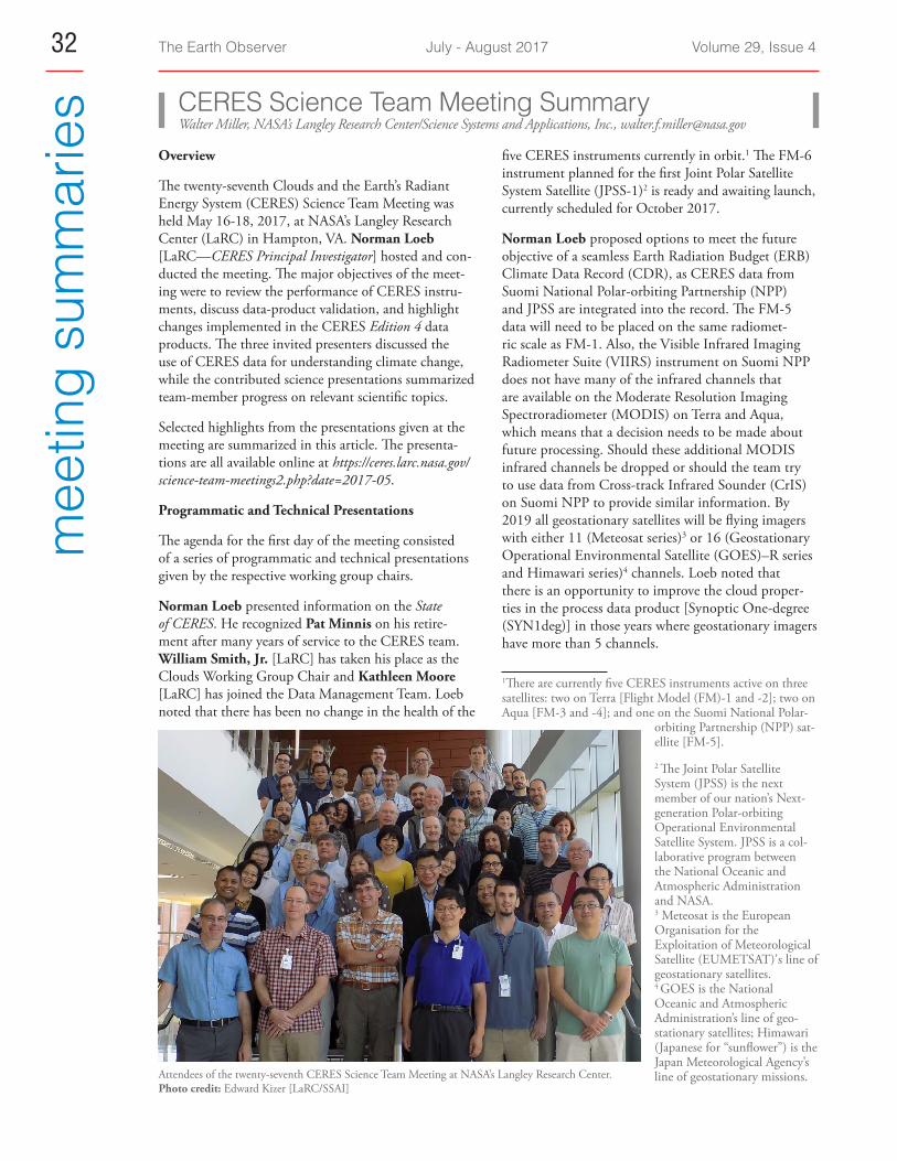
The Earth Observer July - August 2017 Volume 29, Issue 432m

eetin

g su

mm

arie

sfive CERES instruments currently in orbit.1 The FM-6 instrument planned for the first Joint Polar Satellite System Satellite (JPSS-1)2 is ready and awaiting launch, currently scheduled for October 2017.

Norman Loeb proposed options to meet the future objective of a seamless Earth Radiation Budget (ERB) Climate Data Record (CDR), as CERES data from Suomi National Polar-orbiting Partnership (NPP) and JPSS are integrated into the record. The FM-5 data will need to be placed on the same radiomet-ric scale as FM-1. Also, the Visible Infrared Imaging Radiometer Suite (VIIRS) instrument on Suomi NPP does not have many of the infrared channels that are available on the Moderate Resolution Imaging Spectroradiometer (MODIS) on Terra and Aqua, which means that a decision needs to be made about future processing. Should these additional MODIS infrared channels be dropped or should the team try to use data from Cross-track Infrared Sounder (CrIS) on Suomi NPP to provide similar information. By 2019 all geostationary satellites will be flying imagers with either 11 (Meteosat series)3 or 16 (Geostationary Operational Environmental Satellite (GOES)–R series and Himawari series)4 channels. Loeb noted that there is an opportunity to improve the cloud proper-ties in the process data product [Synoptic One-degree (SYN1deg)] in those years where geostationary imagers have more than 5 channels.

1There are currently five CERES instruments active on three satellites: two on Terra [Flight Model (FM)-1 and -2]; two on Aqua [FM-3 and -4]; and one on the Suomi National Polar-

orbiting Partnership (NPP) sat-ellite [FM-5].

2 The Joint Polar Satellite System (JPSS) is the next member of our nation’s Next-generation Polar-orbiting Operational Environmental Satellite System. JPSS is a col-laborative program between the National Oceanic and Atmospheric Administration and NASA.3 Meteosat is the European Organisation for the Exploitation of Meteorological Satellite (EUMETSAT)'s line of geostationary satellites.4 GOES is the National Oceanic and Atmospheric Administration’s line of geo-stationary satellites; Himawari (Japanese for “sunflower”) is the Japan Meteorological Agency’s line of geostationary missions.

CERES Science Team Meeting Summary Walter Miller, NASA’s Langley Research Center/Science Systems and Applications, Inc., walter.f.miller@nasa.gov

Overview

The twenty-seventh Clouds and the Earth’s Radiant Energy System (CERES) Science Team Meeting was held May 16-18, 2017, at NASA’s Langley Research Center (LaRC) in Hampton, VA. Norman Loeb [LaRC—CERES Principal Investigator] hosted and con-ducted the meeting. The major objectives of the meet-ing were to review the performance of CERES instru-ments, discuss data-product validation, and highlight changes implemented in the CERES Edition 4 data products. The three invited presenters discussed the use of CERES data for understanding climate change, while the contributed science presentations summarized team-member progress on relevant scientific topics.

Selected highlights from the presentations given at the meeting are summarized in this article. The presenta-tions are all available online at https://ceres.larc.nasa.gov/science-team-meetings2.php?date=2017-05. 

Programmatic and Technical Presentations

The agenda for the first day of the meeting consisted of a series of programmatic and technical presentations given by the respective working group chairs.

Norman Loeb presented information on the State of CERES. He recognized Pat Minnis on his retire-ment after many years of service to the CERES team. William Smith, Jr. [LaRC] has taken his place as the Clouds Working Group Chair and Kathleen Moore [LaRC] has joined the Data Management Team. Loeb noted that there has been no change in the health of the

Attendees of the twenty-seventh CERES Science Team Meeting at NASA’s Langley Research Center. Photo credit: Edward Kizer [LaRC/SSAI]

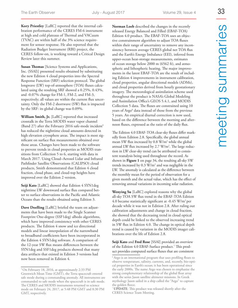
The Earth Observer July - August 2017 Volume 29, Issue 4 33

mee

ting

sum

mar

iesKory Priestley [LaRC] reported that the internal cali-

bration performance of the CERES FM-6 instrument at high and cold plateaus of Thermal and VACuum (TVAC) are within half of the 3% science require-ment for sensor response. He also reported that the Radiation Budget Instrument (RBI) project, the CERES follow-on, is working toward a Critical Design Review later this summer.

Susan Thomas [Science Systems and Applications, Inc. (SSAI)] presented results obtained by substituting the new Edition 4 cloud properties into the Spectral Response Function (SRF) selection protocol. The global longwave (LW) top-of-atmosphere (TOA) fluxes calcu-lated using the resulting SRF showed a 0.25%, 0.43%, and -0.07% change for FM-1, FM-2, and FM-3, respectively; all values are within the current flux uncer-tainty. Only the FM-2 shortwave (SW) flux is impacted by the SRF: its global change was 0.09%.

William Smith, Jr. [LaRC] reported that increased crosstalk in the Terra MODIS water vapor channel (Band 27) after the February 2016 safe-mode incident5 has reduced the nighttime cloud amounts detected in high elevation cryosphere areas. The impact is most sig-nificant on surface flux measurements obtained over those areas. Changes have been made to the software to prevent trends in cloud properties as MODIS tran-sitions from Collection 5 to 6, starting with data in March 2017. Using Cloud–Aerosol Lidar and Infrared Pathfinder Satellite Observations (CALIPSO) cloud products, Smith demonstrated that Edition 4 cloud fraction, cloud phase, and cloud-top heights have improved over the Edition 2 version.

Seiji Kato [LaRC] showed that Edition 4 SYN1deg nighttime LW downward surface flux compared bet-ter to surface observations in the Pacific and Atlantic Oceans than the results obtained using Edition 3.

Dave Doelling [LaRC] briefed the team on adjust-ments that have been made to the Single Scanner Footprint One-degree (SSF1deg) albedo algorithms, which have improved consistency with other CERES products. The Edition 4 snow and ice directional models and linear interpolation of the narrowband to broadband coefficients have been incorporated in the Edition 4 SYN1deg software. A comparison of the 12-year SW flux means differences between the SYN1deg and SSF1deg products showed that many data artifacts that existed in Edition 3 versions had now been removed in Edition 4.

5 On February 18, 2016, at approximately 2:33 PM Greenwich Mean Time (GMT), the Terra spacecraft entered safe mode during a commanding anomaly. All instruments are commanded to safe mode when the spacecraft is in safe mode. The CERES and MODIS instruments returned to science mode on February 24, 2017, at 5:48 PM GMT and 8:30 PM GMT, respectively.

Norman Loeb described the changes in the recently released Energy Balanced and Filled (EBAF-TOA) Edition 4.0 product. The EBAF-TOA uses an objec-tive constrainment algorithm to adjust TOA fluxes within their range of uncertainty to remove any incon-sistency between average CERES global net TOA flux and the Earth’s Energy Imbalance (EEI), inferred from upper-ocean heat-storage measurements, estimates of ocean storage below 2000 m (6562 ft), and atmo-spheric and lithospheric heating. The major improve-ments in the latest EBAF-TOA are the result of includ-ing Edition 4 improvements in instrument calibration, cloud properties, angular directional models (ADMs), and cloud properties derived from hourly geostationary imagery. The meteorological assimilation scheme used throughout the product is NASA’s Global Modeling and Assimilation Office’s GEOS 5.4.1, and MODIS Collection 5 data. The fluxes are constrained using 10 years of Argo6 data instead of those from the previous 5 years. An empirical diurnal correction is now used, based on the difference between the morning and after-noon fluxes, expressed as the ratio of the daily flux.

The Edition 4.0 EBAF-TOA clear-sky fluxes differ mark-edly from Edition 2.8. Specifically, the global annual mean SW flux increased by 0.8 W/m2 while the global annual LW flux increased by 2.7 W/m2. The large reduc-tion in LW clear-sky trend can be attributed to consis-tent reanalysis being used throughout the record. As shown in Figure 1 on page 34, the resulting all-sky SW trends increased by 0.3 W/m2 and was negligible in the LW. The anomaly is calculated as the difference between the monthly mean for the period of observation for a given month and the actual value, which has the effect of removing annual variations in incoming solar radiation.

Wenying Su [LaRC] explored reasons why the global all-sky TOA SW flux trend in the EBAF-TOA Edition 4.0 became statistically significant at -0.45 W/m2 per decade while it was not in Edition 2.8. After ruling out calibration adjustments and change in cloud fraction, she showed that the decreasing trend in cloud optical depth could be linked to the observed increasing trend in SW flux in Edition 4.0. The change in optical depth trend is caused by variation in the MODIS imager cali-brations over the life of Edition 2.8.

Seiji Kato and Fred Rose [SSAI] provided an overview of the Edition 4.0 EBAF-Surface product.7 This prod-uct provides computed surface fluxes that are consistent 6 Argo is an international program that uses profiling floats to observe temperature, salinity, currents, and, recently, bio-opti-cal properties in Earth’s ocean; it has been operational since the early 2000s. The name Argo was chosen to emphasize the strong complementary relationship of the global float array with the series Jason satellite altimeter missions. In Greek mythology Jason sailed in a ship called the “Argo” to capture the golden fleece. 7 UPDATE: This product was released shortly after the CERES Science Team Meeting.

The Earth Observer July - August 2017 Volume 29, Issue 434m

eetin

g su

mm

arie

s

with the EBAF-TOA product. Again, this EBAF-Surface product takes advantage of all the Edition 4 improve-ments in the CERES product line. The increase in cloud fraction derived from both MODIS and geostationary imagers have a large effect on the SW surface down-welling flux, but have largely been removed through bias correction. The clear-sky mean differences are consistent with the reduction in clear-area sampling.

Kathleen Moore talked about the upcoming delivery of software to support Edition 4 SYN1deg and the changes for using MODIS Collection 6 in creation of the SSF. With the completion of Edition 3 processing in June 2017, about a third of the current software can be deprecated.

Jeff Walter [LaRC] then described the Atmospheric Data Science Center (ASDC) cloud-strategy roadmap that will incorporate current business practices for data centers. Both Moore and Walter then discussed the evolution of the CERES production system. They have been meeting with stakeholders to capture the needs of an updated architecture and investigating NASA/Jet Propulsion Laboratory’s Hybrid-cloud Science Data System (HySDS)8 to automate processing if a cloud environment is used.

Jessica Taylor [LaRC] brought the team up to date on Citizen Science efforts. One focus is on develop-ing a communication plan for the coming launch of FM-6 on JPSS-1, including interviews with team members. Taylor and her colleagues are looking at ideas that can tie CERES to this summer’s total solar eclipse on August 21. She highlighted a Bulletin of the American Meteorological Society article on the twentieth

8 HySDS manages the use of on-premise cloud computing resources at JPL, and also has the ability to gain additional compute resources from the commercial cloud when needed to meet processing demands.

anniversary of the Student’s Cloud Observation OnLine (S’COOL) program, noting that 150,000 observa-tions have been received during that time. S’COOL has now been absorbed into the Global Learning and Observations to benefit the Environment (GLOBE) Program, which will bring additional focus to the pro-gram, including blogs and applications.

Paul Stackhouse [LaRC] reported on feedback from a user of the data that showed how power produc-tion from four solar panel fields tracked with the CERES Fast Longwave and Shortwave Radiative Fluxes (FLASHFlux) SW flux during Hurricane Matthew in 2016. He reported only minor differences were observed in the transition from MODIS Collection 5 to Collection 6 data.

Invited Science Presentations

There were three invited presentations on the morning of the meeting’s second day. Each of the presenters dis-cussed changes to major climate models, and how satel-lite observations can be used to evaluate them.

Yi Ming [Geophysical Fluid Dynamics Laboratory (GFDL)] provided information on the GFDL’s next generation Coupled Physical Model 4 (CM4), which uses a cubed-sphere, finite-volume dynamical core with 50- or 100-km (~31- to 62-mi) resolution and 32 or 48 vertical layers with updated physics to handle precipita-tion. It showed an ~40% reduction in measured global differences in both SW and LW radiation when com-pared with EBAF-TOA Edition 2.8 observations. The time series between the modeled and observed radiation had good correlation (between 0.54 and 0.79, depend-ing on the variable). He suggested that even more syn-ergy between model and satellite products like CERES can be achieved.

Figure 1. Trends from the Energy Balanced and Filled (EBAF) Top of Atmosphere (TOA) Edition 4 prod-uct. Shown are the: SW all-sky flux anomaly in Edition 4.0 [top left]; dif-ference in the SW all-sky flux anom-aly between Edition 4.0 and 2.8 [top right]; LW all-sky flux anomaly in Edition 4.0 [center left]; difference in the LW all-sky flux anomaly between Edition 4.0 and 2.8 [center right]; net all-sky flux anomaly in Edition 4.0 [bottom left]; difference in the net all-sky flux anomaly between Edition 4.0 and 2.8 [bottom right]. See Norman Loeb’s presentation summary on page 33 for further explanation. Image credit: Norman Loeb

The Earth Observer July - August 2017 Volume 29, Issue 4 35

mee

ting

sum

mar

iesAndrew Gettelman [National Center of Atmospheric

Research (NCAR)] evaluated the performance of the Community Earth System Model 2 (CESM 2) by look-ing at radiation forcing and feedback. The model is much improved from the previous version, but there are still biases in the Arctic that can likely be attributed to the inadequate representation of clouds and their microphysical properties in the model. The Equilibrium Climate Sensitivity (ECS) remains similar to the earlier version. The model has a lower Ocean Heat Uptake and TOA imbalance than what is observed.

Ralph Kahn [NASA’s Goddard Space Flight Center (GSFC)] examined the impact of more realistic repre-sentations of aerosol thickness and coverage within the Coupled Model Intercomparison Project 5 (CMIP 5) models and resulting improvements in its radiation budget calculations. He gave details on improvements in aerosol measurements derived from the Multi-angle Imaging Spectroradiometer (MISR) on Terra that have higher resolution and improved performance relative to Aerosol Robotic Network (AERONET)9 and air-craft measurements.9 AERONET is an federated worldwide network of automated ground-based sun photometers. To learn more visit https://aeronet.gsfc.nasa.gov.

Contributed Science Presentations

The many contributed science presentations on the sec-ond and third days of the meeting addressed a variety of topics. These included:

• methods to estimate climate sensitivity;

• comparison of observation to climate models;

• validation efforts, where CERES cloud properties are compared with surface and cloud observations or other satellite products;

• improvements to existing Earth Radiation Budget products;

• efforts to improve algorithms for future CERES products; and

• use of machine learning to improve current algorithms.

For a summary of these presentations, see the Table, which begins below and continues on the next page.

Table. List of contributed science presentations at the twenty-seventh CERES Science Team Meeting.Speaker [Affiliation] Summary

Andrew Dessler [Texas A&M University]

Showed that the 500-hPa (mb) tropical temperature is a better choice than surface temperature to compare with CERES measurements of change in radiation to determine Equilibrium Climate Sensitivity (ECS).

Lazaros Oreopoulos [NASA’s Goddard Space Flight Center (GSFC)]

Discussed the relative importance of various cloud regimes and cloud vertical structure (inferred vertical velocity) on the CERES Net Cloud Radiative Effect.*

Patrick Taylor [NASA’s Langley Research Center (LaRC)]

Showed a strong inverse correlation between clouds and sea ice concentration (i.e., less ice will result in more clouds) during autumn. A sea ice reduction in fall and the increased cloud response could delay the fall freeze-up.

Brad Hegyi [Universities Space Research Association]

Showed that winter sea ice growth reduces during periods with nega-tive Arctic Dipole (which transports warm, moist air into the Arctic, thus increasing surface downwelling LW fluxes). By comparison, the phase of Arctic Oscillation shows no significant correlation to sea ice growth.

Xiuhong Chen [University of Michigan]

Showed that using the LW upwelling flux to estimate surface temperature provides better agreement between the data from Atmospheric Infrared Sounder (AIRS) on Aqua and clear-sky radiance measurements taken at the Department of Energy’s Atmospheric Radiation Measurement (ARM) Southern Great Plains (SGP) site.

Seung–See Ham [LaRC/Science Systems and Applications, Inc (SSAI)]

Examined sensitivity of clear-sky flux to different Global Modeling and Assimilation Office (GMAO) datasets.

Ping Yang [Texas A&M]

Showed that the overall performance of cloud properties from the new two-habit model is similar to results obtained using data from MODIS Collection 6. He also showed preliminary results in creating a new data-base of African and Asian dust optical properties.

* CERES net Cloud Radiative Effect is the net impact of a cloud on climate—i.e., warming caused by outgoing longwave (LW) infrared radiative flux at the top of the atmosphere (TOA) compared to cooling from shortwave (SW) solar radiative flux back to space to cool the Earth as a difference from what occurs if no clouds are present.

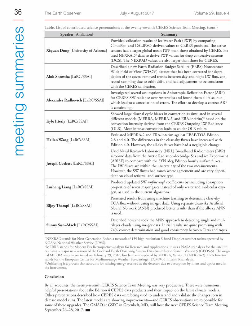
The Earth Observer July - August 2017 Volume 29, Issue 436m

eetin

g su

mm

arie

s Table. List of contributed science presentations at the twenty-seventh CERES Science Team Meeting. (cont.)

Speaker [Affiliation] Summary

Xiquan Dong [University of Arizona]

Provided validation results of Ice Water Path (IWP) by comparing CloudSat- and CALIPSO-derived values to CERES products. The active sensors had a larger global mean IWP than those obtained by CERES. He used NEXRAD† data to derive IWP values for deep convective systems (DCS). The NEXRAD values are also larger than those for CERES.

Alok Shrestha [LaRC/SSAI]

Described a new Earth Radiation Budget Satellite (ERBS) Nonscanner Wide Field of View (WFOV) dataset that has been corrected for degra-dation of the cover, removed trends between day and night LW flux, cor-rected sampling due to orbit drift, and had adjustment to be consistent with the CERES calibration.

Alexander Radkevich [LaRC/SSAI]

Investigated several assumptions in Anisotropic Reflection Factor (ARF) for CERES SW radiance over Antarctica and found them all false, but which lead to a cancellation of errors. The effort to develop a correct ARF is continuing.

Kyle Itterly [LaRC/SSAI]

Showed large diurnal cycle biases in convection as simulated in several different models (MERRA, MERRA-2, and ERA-interim)‡ based on the convection intensity derived from the CERES Outgoing LW Radiance (OLR). More intense convection leads to colder OLR values.

Hailan Wang [LaRC/SSAI]Evaluated MERRA-2 and ERA-interim against EBAF-TOA Edition 2.8 and 4.0. The differences in the clear-sky fluxes have increased with Edition 4.0. However, the all-sky fluxes have had a negligible change.

Joseph Corbett [LaRC/SSAI]

Used Naval Research Laboratory (NRL) Broadband Radiometers (BBR) airborne data from the Arctic Radiation-Icebridge Sea and ice Experiment (ARISE) to compare with the SYN1deg Edition hourly surface fluxes. The LW fluxes are within the uncertainty of the two measurements. However, the SW fluxes had much worse agreement and are very depen-dent on cloud retireval and surface type.

Lusheng Liang [LaRC/SSAI]Produced updated SW unfiltering§ coefficients by including absorption properties of seven major gases instead of only water and molecular oxy-gen, as used in the current algorithm.

Bijoy Thampi [LaRC/SSAI]

Presented results from using machine learning to determine clear-sky TOA flux without using imager data. Using separate clear-sky Artificial Neural Network (ANN) produced better results than if the all-sky ANN is used.

Sunny Sun–Mack [LaRC/SSAI]Described how she took the ANN approach to detecting single and mul-tilayer clouds using imager data. Initial results are quite promising with 74% correct determination and good consistency between Terra and Aqua.

† NEXRAD stands for Next-Generation Radar, a network of 159 high-resolution S-band Doppler weather radars operated by NOAA’s National Weather Service (NWS).‡ MERRA stands for Modern Era Retrospective-analysis for Research and Applications; it was a NASA reanalysis for the satellite era using a major new version of the Goddard Earth Observing System Data Assimilation System Version 5 (GEOS-5). The origi-nal MERRA was discontinued on February 29, 2016, but has been replaced by MERRA, Version 2 (MERRA-2). ERA Interim stands for the European Center for Medium-range Weather Forecasting’s (ECMWF) Interim Reanalysis. § Unfiltering is a process that accounts for missing energy received at the detector due to absorption by filters and optics used in the instrument.

Conclusion

By all accounts, the twenty-seventh CERES Science Team Meeting was very productive. There were numerous helpful presentations about the Edition 4 CERES data products and their impact on the latest climate models. Other presentations described how CERES data were being used to understand and validate the changes seen in climate model runs. The latest models are showing improvements—and CERES observations are responsible for some of these upgrades. The GMAO at GSFC in Greenbelt, MD, will host the next CERES Science Team Meeting September 26–28, 2017.

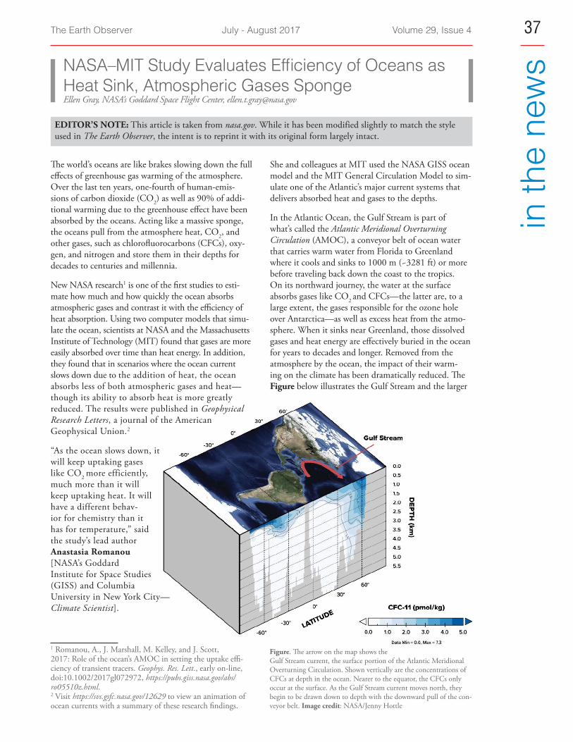
The Earth Observer July - August 2017 Volume 29, Issue 4 37

in th

e ne

ws

Figure. The arrow on the map shows the Gulf Stream current, the surface portion of the Atlantic Meridional Overturning Circulation. Shown vertically are the concentrations of CFCs at depth in the ocean. Nearer to the equator, the CFCs only occur at the surface. As the Gulf Stream current moves north, they begin to be drawn down to depth with the downward pull of the con-veyor belt. Image credit: NASA/Jenny Hottle

The world’s oceans are like brakes slowing down the full effects of greenhouse gas warming of the atmosphere. Over the last ten years, one-fourth of human-emis-sions of carbon dioxide (CO2) as well as 90% of addi-tional warming due to the greenhouse effect have been absorbed by the oceans. Acting like a massive sponge, the oceans pull from the atmosphere heat, CO2, and other gases, such as chlorofluorocarbons (CFCs), oxy-gen, and nitrogen and store them in their depths for decades to centuries and millennia.

New NASA research1 is one of the first studies to esti-mate how much and how quickly the ocean absorbs atmospheric gases and contrast it with the efficiency of heat absorption. Using two computer models that simu-late the ocean, scientists at NASA and the Massachusetts Institute of Technology (MIT) found that gases are more easily absorbed over time than heat energy. In addition, they found that in scenarios where the ocean current slows down due to the addition of heat, the ocean absorbs less of both atmospheric gases and heat—though its ability to absorb heat is more greatly reduced. The results were published in Geophysical Research Letters, a journal of the American Geophysical Union.2

“As the ocean slows down, it will keep uptaking gases like CO2 more efficiently, much more than it will keep uptaking heat. It will have a different behav-ior for chemistry than it has for temperature,” said the study’s lead author Anastasia Romanou [NASA’s Goddard Institute for Space Studies (GISS) and Columbia University in New York City—Climate Scientist].

1 Romanou, A., J. Marshall, M. Kelley, and J. Scott, 2017: Role of the ocean’s AMOC in setting the uptake effi-ciency of transient tracers. Geophys. Res. Lett., early on-line, doi:10.1002/2017gl072972, https://pubs.giss.nasa.gov/abs/ro05510z.html.2 Visit https://svs.gsfc.nasa.gov/12629 to view an animation of ocean currents with a summary of these research findings.

EDITOR’S NOTE: This article is taken from nasa.gov. While it has been modified slightly to match the style used in The Earth Observer, the intent is to reprint it with its original form largely intact.

NASA–MIT Study Evaluates Efficiency of Oceans as Heat Sink, Atmospheric Gases Sponge Ellen Gray, NASA’s Goddard Space Flight Center, ellen.t.gray@nasa.gov

She and colleagues at MIT used the NASA GISS ocean model and the MIT General Circulation Model to sim-ulate one of the Atlantic’s major current systems that delivers absorbed heat and gases to the depths.

In the Atlantic Ocean, the Gulf Stream is part of what’s called the Atlantic Meridional Overturning Circulation (AMOC), a conveyor belt of ocean water that carries warm water from Florida to Greenland where it cools and sinks to 1000 m (~3281 ft) or more before traveling back down the coast to the tropics. On its northward journey, the water at the surface absorbs gases like CO2 and CFCs—the latter are, to a large extent, the gases responsible for the ozone hole over Antarctica—as well as excess heat from the atmo-sphere. When it sinks near Greenland, those dissolved gases and heat energy are effectively buried in the ocean for years to decades and longer. Removed from the atmosphere by the ocean, the impact of their warm-ing on the climate has been dramatically reduced. The Figure below illustrates the Gulf Stream and the larger

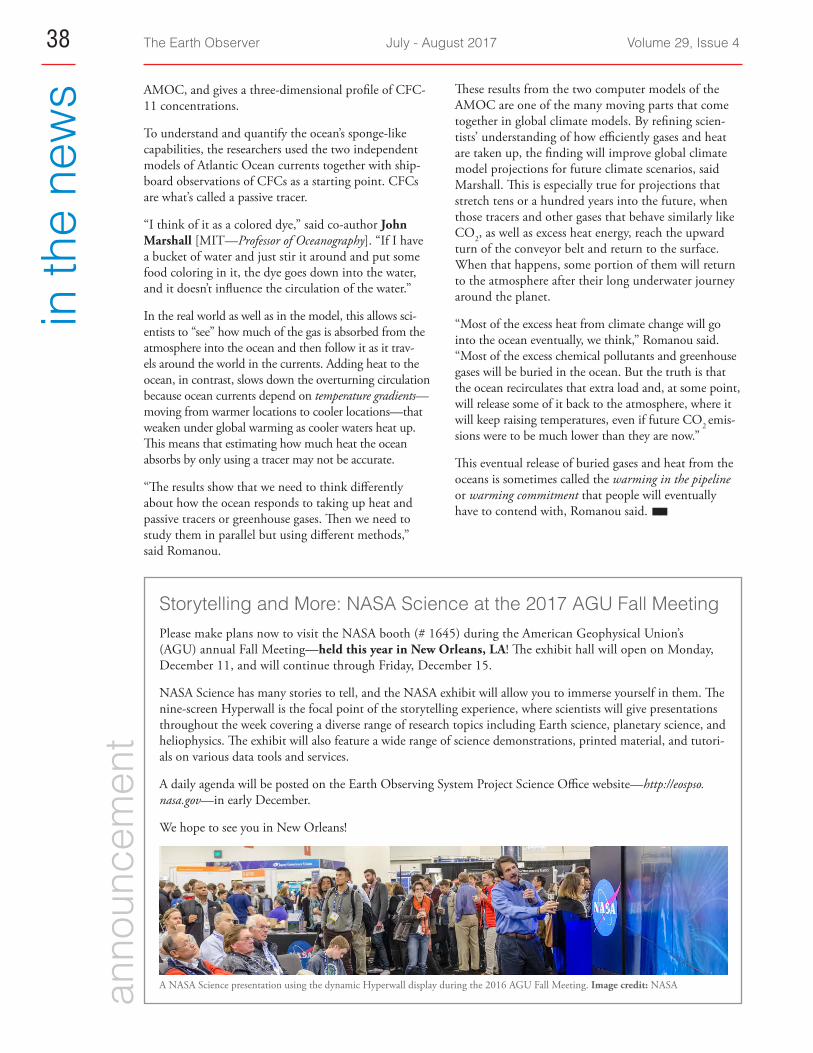
The Earth Observer July - August 2017 Volume 29, Issue 438in

the

new

s AMOC, and gives a three-dimensional profile of CFC-11 concentrations.

To understand and quantify the ocean’s sponge-like capabilities, the researchers used the two independent models of Atlantic Ocean currents together with ship-board observations of CFCs as a starting point. CFCs are what’s called a passive tracer.

“I think of it as a colored dye,” said co-author John Marshall [MIT—Professor of Oceanography]. “If I have a bucket of water and just stir it around and put some food coloring in it, the dye goes down into the water, and it doesn’t influence the circulation of the water.”

In the real world as well as in the model, this allows sci-entists to “see” how much of the gas is absorbed from the atmosphere into the ocean and then follow it as it trav-els around the world in the currents. Adding heat to the ocean, in contrast, slows down the overturning circulation because ocean currents depend on temperature gradients—moving from warmer locations to cooler locations—that weaken under global warming as cooler waters heat up. This means that estimating how much heat the ocean absorbs by only using a tracer may not be accurate.

“The results show that we need to think differently about how the ocean responds to taking up heat and passive tracers or greenhouse gases. Then we need to study them in parallel but using different methods,” said Romanou.

These results from the two computer models of the AMOC are one of the many moving parts that come together in global climate models. By refining scien-tists’ understanding of how efficiently gases and heat are taken up, the finding will improve global climate model projections for future climate scenarios, said Marshall. This is especially true for projections that stretch tens or a hundred years into the future, when those tracers and other gases that behave similarly like CO2, as well as excess heat energy, reach the upward turn of the conveyor belt and return to the surface. When that happens, some portion of them will return to the atmosphere after their long underwater journey around the planet.

“Most of the excess heat from climate change will go into the ocean eventually, we think,” Romanou said. “Most of the excess chemical pollutants and greenhouse gases will be buried in the ocean. But the truth is that the ocean recirculates that extra load and, at some point, will release some of it back to the atmosphere, where it will keep raising temperatures, even if future CO2 emis-sions were to be much lower than they are now.”

This eventual release of buried gases and heat from the oceans is sometimes called the warming in the pipeline or warming commitment that people will eventually have to contend with, Romanou said.

Storytelling and More: NASA Science at the 2017 AGU Fall Meeting Please make plans now to visit the NASA booth (# 1645) during the American Geophysical Union’s (AGU) annual Fall Meeting—held this year in New Orleans, LA! The exhibit hall will open on Monday, December 11, and will continue through Friday, December 15.

NASA Science has many stories to tell, and the NASA exhibit will allow you to immerse yourself in them. The nine-screen Hyperwall is the focal point of the storytelling experience, where scientists will give presentations throughout the week covering a diverse range of research topics including Earth science, planetary science, and heliophysics. The exhibit will also feature a wide range of science demonstrations, printed material, and tutori-als on various data tools and services.

A daily agenda will be posted on the Earth Observing System Project Science Office website—http://eospso. nasa.gov—in early December.

We hope to see you in New Orleans!

anno

unce

men

t

A NASA Science presentation using the dynamic Hyperwall display during the 2016 AGU Fall Meeting. Image credit: NASA

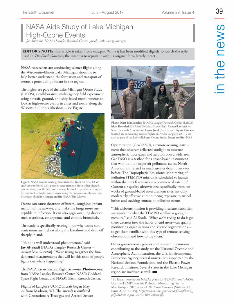
The Earth Observer July - August 2017 Volume 29, Issue 4 39

in th

e ne

ws

EDITOR’S NOTE: This article is taken from nasa.gov. While it has been modified slightly to match the style used in The Earth Observer, the intent is to reprint it with its original form largely intact.

NASA Aids Study of Lake Michigan High-Ozone Events Joe Atkinson, NASA’s Langley Research Center, joseph.s.atkinson@nasa.gov

NASA researchers are conducting science flights along the Wisconsin–Illinois Lake Michigan shoreline to help better understand the formation and transport of ozone, a potent air pollutant in the region.

The flights are part of the Lake Michigan Ozone Study (LMOS), a collaborative, multi-agency field experiment using aircraft, ground, and ship-based measurements to look at high-ozone events in cities and towns along the Wisconsin–Illinois lakeshore—see Figure.

Ozone can cause shortness of breath, coughing, inflam-mation of the airways, and make the lungs more sus-ceptible to infection. It can also aggravate lung diseases such as asthma, emphysema, and chronic bronchitis.

The study is specifically zeroing in on why ozone con-centrations are highest along the lakeshore and drop off sharply inland.

“It’s not a well understood phenomenon,” said Jay Al-Saadi [NASA’s Langley Research Center—Atmospheric Scientist]. “We’re trying to gather the fun-damental measurements that will let this team of people figure out what’s happening.”

The NASA researchers and flight crew—see Photo—come from NASA’s Langley Research Center, NASA’s Goddard Space Flight Center, and NASA’s Glenn Research Center.

Flights of Langley’s UC-12 aircraft began May 22 from Madison, WI. The aircraft is outfitted with Geostationary Trace gas and Aerosol Sensor

Optimization (GeoTASO), a remote-sensing instru-ment that observes reflected sunlight to measure atmospheric trace gases and aerosols over a wide area. GeoTASO is a testbed for a space-based instrument that will monitor major air pollutants across North America hourly and in much greater detail than ever before. The Tropospheric Emissions: Monitoring of Pollution (TEMPO) mission is scheduled to launch within the next few years on a commercial satellite.1 Current air quality observations, specifically from net-works of ground-based measurement sites, are only moderately effective at monitoring exposure to air pol-lution and tracking sources of pollution events.

“This airborne mission is providing measurements that are similar to what the TEMPO satellite is going to measure,” said Al-Saadi. “What we’re trying to do is get these datasets into the hands of end users—air quality monitoring organizations and science organizations—to get them familiar with this type of remote-sensing observations and how to use them.”

Other government agencies and research institutions contributing to the study are the National Oceanic and Atmospheric Administration, the U.S. Environmental Protection Agency, several universities supported by the National Science Foundation, and the Electric Power Research Institute. Several states in the Lake Michigan region are involved as well. 1 To learn more about NASA’s plans for TEMPO, see “NASA Ups the TEMPO on Air Pollution Monitoring” in the March–April 2013 issue of The Earth Observer [Volume 25, Issue 2, pp. 10-15], https://eospso.nasa.gov/sites/default/files/eo_pdfs/March_April_2013_508_color.pdf].

Figure. NASA remote sensing measurements from the UC-12 air-craft are combined with partner measurements from other aircraft, ground sites, mobile labs, and a research vessel to provide a compre-hensive look at high-ozone events along the Wisconsin–Illinois Lake Michigan shoreline. Image credit: NASA/Tim Marvel

Photo. Kurt Blankenship [NASA’s Langley Research Center (LaRC)], Matt Kowaleski [NASA’s Goddard Space Flight Center/Universities Space Research Association], Laura Judd [LaRC], and Taylor Thorson [LaRC] are conducting science flights on NASA Langley’s UC-12 air-craft as part of the Lake Michigan Ozone Study. Image credit: NASA

The Earth Observer July - August 2017 Volume 29, Issue 440in

the

new

s

A new study suggests that most global climate mod-els may underestimate the amount of rain that will fall in Earth’s tropical regions as our planet continues to warm. That’s because these models underestimate decreases in high clouds over the tropics seen in recent NASA observations, according to research led by scien-tist Hui Su [NASA/Jet Propulsion Laboratory (JPL)].

Wait a minute: How can fewer clouds lead to more rain-fall? Globally, rainfall isn’t related just to the clouds that are available to make rain but also to Earth’s energy bud-get—incoming energy from the sun compared to outgo-ing heat energy. High-altitude tropical clouds trap heat in the atmosphere. If there are fewer of these clouds in the future, the tropical atmosphere will cool. Judging from observed changes in clouds over recent decades, it appears that the atmosphere would create fewer high clouds in response to surface warming. It would also increase tropical rainfall, which would warm the air to balance the cooling from the high cloud shrinkage.  

Rainfall warming the air also sounds counterintuitive—people are used to rain cooling the air around them, not warming it. Several miles up in the atmosphere, how-ever, a different process prevails. When water evaporates into water vapor here on Earth’s surface and rises into the atmosphere, it carries with it the heat energy that made it evaporate. In the cold upper atmosphere, when the water vapor condenses into liquid droplets or ice particles, it releases its heat and warms the atmosphere.

The new study, titled “Tightening of Tropical Ascent and High Clouds Key to Precipitation Change in a Warmer Climate,”1 is published in the journal Nature Communications. It puts the decrease in high tropi-cal cloud cover in context as one result of a planet-wide shift in large-scale air flows that is occurring as Earth’s surface temperature warms. These large-scale flows are called the atmospheric general circulation, and they include a wide zone of rising air centered on the equator. Observations over the last 30 to 40 years have shown that this zone is narrowing as the climate warms, causing the decrease in high clouds.

Su and colleagues at JPL and four universities compared climate data from the past few decades with 23 climate model simulations of the same period. Climate mod-elers use retrospective simulations like these to check 1 Hui Su spoke on this topic at the recent A-Train Symposium; a summary appears on page 4 of this issue.

EDITOR’S NOTE: This article is taken from nasa.gov. While it has been modified slightly to match the style used in The Earth Observer, the intent is to reprint it with its original form largely intact.

NASA Data Suggest Future May Be Rainier Than Expected Carol Rasmussen, NASA/Jet Propulsion Laboratory, carol.m.rasmussen@jpl.nasa.gov

how well their numerical models are able to reproduce observations. For data, the team used observations of outgoing thermal radiation from NASA’s space-borne Clouds and the Earth’s Radiant Energy System (CERES) and other satellite instruments, as well as ground-level observations.

Su’s team found that most of the climate models under-estimated the rate of increase in precipitation for each degree of surface warming that has occurred in recent decades. The models that came closest to match-ing observations of clouds in the present-day climate showed a greater precipitation increase for the future than the other models.

Su said that by tracing the underestimation problem back to the models’ deficiencies in representing tropi-cal high clouds and the atmospheric general circulation, “This study provides a pathway for improving predic-tions of future precipitation change.”

Tropical rainfall may increase more than previously thought as the cli-mate warms. Photo credit: teresaaaa, CC BY-ND 2.0

The Earth Observer July - August 2017 Volume 29, Issue 4 41

NA

SA e

arth

sci

ence

in th

e ne

ws

NASA Earth Science in the NewsSamson Reiny, NASA’s Earth Science News Team, samson.k.reiny@nasa.gov

How NASA Tracks This Iceberg Through The Dark Antarctic Night, July 6, inverse.com. An iceberg as big as Delaware is about to break free from the Antarctic Peninsula—but no one will see it. Antarctica is in the depths of dark winter, and much of the continent will not see daylight again for weeks. At the Larsen C ice shelf, which is close to the continent’s most northerly tip, the sun might graze the horizon for a couple of hours at midday before dipping back down for another long night. For this reason, planes don’t fly over Antarctica in the wintertime, barring extraordinary cir-cumstances. And yet, we’ll know when this behemoth slab of ice calves from the shelf and drifts off into the Southern Ocean, and we’ll know which direction it heads. We will know thanks to NASA and European Space Agency (ESA) satellites, which use clever work-arounds to see what cannot be seen. In June, NASA peered through the darkness with its Landsat 8 satel-lite. It used infrared thermal sensors to visualize the rift between the iceberg and the ice shelf, which only

has five miles to go before separation is complete—see Figure 1. The thermal sensors exploit the difference in temperature between the ocean and the ice surface, which is colder than the open water.1

Global Drop In Wildfires Results In Lower Emissions But Threatens Life On The Savannah, July 3, cosmosmagazine.com. The number of bush and grass fires across the globe has declined by almost a quarter in less than two decades—but that’s not necessarily all good news. Using data from several satellites gathered over the past 18 years, researchers at NASA’s Goddard Space Flight Center (GSFC), found the total area burnt each year has dropped by about 24%. In a paper published in the journal Science, lead researcher Niels Andela [GSFC] and colleagues note that the largest

1 UPDATE: Sometime between July 10 and July 12, 2017, an iceberg about the size of Delaware split off from Antarctica’s Larsen C ice shelf. To view images of the new iceberg, visit https://earthobservatory.nasa.gov/IOTD/view.php?id=90557.

Figure 1. On June 17, 2017, the Thermal Infrared Sensor (TIRS) on Landsat 8 captured a false-color image of the crack and the surrounding ice shelf. It shows the relative warmth or coolness of the landscape. Orange depicts where the surface is the warmest, most notably the areas of open ocean and of water topped by thin sea ice. Light blues and whites are the coldest areas, spanning most of the ice shelf and some areas of sea ice. Credit: NASA’s Earth Observatory

N

A-57B

Sea ice

Thin sea ice

Crack

10 km

Thermal Signature

Colder Warmer

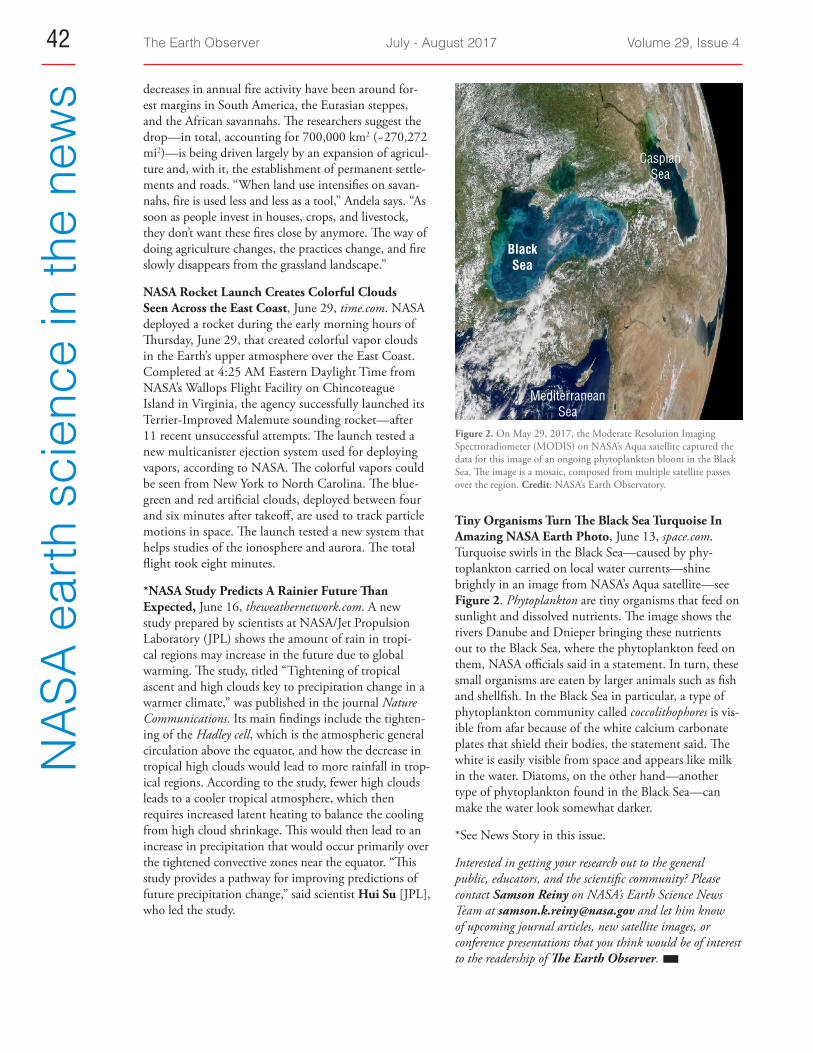
The Earth Observer July - August 2017 Volume 29, Issue 442N

ASA

ear

th s

cien

ce in

the

new

s decreases in annual fire activity have been around for-est margins in South America, the Eurasian steppes, and the African savannahs. The researchers suggest the drop—in total, accounting for 700,000 km2 (~270,272 mi2)—is being driven largely by an expansion of agricul-ture and, with it, the establishment of permanent settle-ments and roads. “When land use intensifies on savan-nahs, fire is used less and less as a tool,” Andela says. “As soon as people invest in houses, crops, and livestock, they don’t want these fires close by anymore. The way of doing agriculture changes, the practices change, and fire slowly disappears from the grassland landscape.”

NASA Rocket Launch Creates Colorful Clouds Seen Across the East Coast, June 29, time.com. NASA deployed a rocket during the early morning hours of Thursday, June 29, that created colorful vapor clouds in the Earth’s upper atmosphere over the East Coast. Completed at 4:25 AM Eastern Daylight Time from NASA’s Wallops Flight Facility on Chincoteague Island in Virginia, the agency successfully launched its Terrier-Improved Malemute sounding rocket—after 11 recent unsuccessful attempts. The launch tested a new multicanister ejection system used for deploying vapors, according to NASA. The colorful vapors could be seen from New York to North Carolina. The blue-green and red artificial clouds, deployed between four and six minutes after takeoff, are used to track particle motions in space. The launch tested a new system that helps studies of the ionosphere and aurora. The total flight took eight minutes.

*NASA Study Predicts A Rainier Future Than Expected, June 16, theweathernetwork.com. A new study prepared by scientists at NASA/Jet Propulsion Laboratory (JPL) shows the amount of rain in tropi-cal regions may increase in the future due to global warming. The study, titled “Tightening of tropical ascent and high clouds key to precipitation change in a warmer climate,” was published in the journal Nature Communications. Its main findings include the tighten-ing of the Hadley cell, which is the atmospheric general circulation above the equator, and how the decrease in tropical high clouds would lead to more rainfall in trop-ical regions. According to the study, fewer high clouds leads to a cooler tropical atmosphere, which then requires increased latent heating to balance the cooling from high cloud shrinkage. This would then lead to an increase in precipitation that would occur primarily over the tightened convective zones near the equator. “This study provides a pathway for improving predictions of future precipitation change,” said scientist Hui Su [JPL], who led the study.

Tiny Organisms Turn The Black Sea Turquoise In Amazing NASA Earth Photo, June 13, space.com. Turquoise swirls in the Black Sea—caused by phy-toplankton carried on local water currents—shine brightly in an image from NASA’s Aqua satellite—see Figure 2. Phytoplankton are tiny organisms that feed on sunlight and dissolved nutrients. The image shows the rivers Danube and Dnieper bringing these nutrients out to the Black Sea, where the phytoplankton feed on them, NASA officials said in a statement. In turn, these small organisms are eaten by larger animals such as fish and shellfish. In the Black Sea in particular, a type of phytoplankton community called coccolithophores is vis-ible from afar because of the white calcium carbonate plates that shield their bodies, the statement said. The white is easily visible from space and appears like milk in the water. Diatoms, on the other hand—another type of phytoplankton found in the Black Sea—can make the water look somewhat darker.

*See News Story in this issue.

Interested in getting your research out to the general public, educators, and the scientific community? Please contact Samson Reiny on NASA’s Earth Science News Team at samson.k.reiny@nasa.gov and let him know of upcoming journal articles, new satellite images, or conference presentations that you think would be of interest to the readership of The Earth Observer.

Figure 2. On May 29, 2017, the Moderate Resolution Imaging Spectroradiometer (MODIS) on NASA’s Aqua satellite captured the data for this image of an ongoing phytoplankton bloom in the Black Sea. The image is a mosaic, composed from multiple satellite passes over the region. Credit: NASA’s Earth Observatory.

Caspian Sea

Black Sea

Mediterranean Sea

The Earth Observer July - August 2017 Volume 29, Issue 4 43

scie

nce

cale

ndar

sEOS Science CalendarSeptember 12–14, 2017 OMI Science Team Meeting, Greenbelt, MD. http://projects.knmi.nl/omi/research/project/meetings/ostm20/details.php

September 26–28, 2017 CERES Science Team Meeting, Greenbelt, MD. https://ceres.larc.nasa.gov/science-team-meetings2.php

October 3–4, 2017 DSCOVR EPIC/NISTAR Science Team Meeting, Greenbelt, MD.

October 10–12, 2017 GRACE Science Team Meeting, Austin, TX. http://www2.csr.utexas.edu/grace/GSTM/

October 23–27, 2017 Ocean Surface Topography Science Team Meeting, Miami, FL. https://cpaess.ucar.edu/meetings/2017/ocean-surface-topog-raphy-science-team-meeting-ostst

January 23–26, 2018 ABovE Science Team Meeting, Seattle, WA https://above.nasa.gov/meetings.html

March 19–23, 2018 2018 Sun-Climate Symposium, Lake Arrowhead, CA. http://lasp.colorado.edu/home/sorce/news-events/meetings/2018-scs

June 4–6, 2018 ASTER Science Team Meeting Tokyo, Japan

Global Change Calendar August 6–11, 2017 Annual Meeting Asia Oceania Geosciences Society, Singapore. http://www.asiaoceania.org/aogs2017/public.asp?page=home.htm

December 11–15, 2017 AGU Fall Meeting, New Orleans, LA. http://fallmeeting.agu.org/2016/2017-fall-meeting-new-orleans

October 22–25, 2017 Geological Society of America Annual Meeting, Seattle, WA. http://community.geosociety.org/gsa2017/home

February 11–16, 2018 Ocean Sciences Meeting, Portland, OR. http://osm.agu.org/2018

Undefined Acronyms Used in Editorial

NOAA National Oceanic and Atmospheric Administration

CSA Canadian Space Agency

CNES Centre National d’Etudes Spatiales (CNES) [French Space Agency]

CS Continuity of Service

ESA European Space Agency

EUMETSAT European Organisation for the Exploitation of Meteorological Satellites

GSFC NASA’s Goddard Space Flight Center

ISS International Space Station

JPL NASA/Jet Propulsion Laboaratory

KSC NASA’s Kennedy Space Center

UKSA United Kingdom Space Agency

WFF NASA’s Wallops Flight Facility

Code 610 National Aeronautics and Space Administration

Goddard Space Flight Center Greenbelt, MD 20771

Official Business Penalty for Private Use: $300

PRSRT STD Postage and Fees Paid National Aeronautics and Space Administration Permit 396

(affix mailing label here)

eos.nasa.govThe Earth Observer

The Earth Observer is published by the Science Communication Support Office, Code 610, NASA’s Goddard Space Flight Center, Greenbelt, Maryland 20771, telephone (301) 614-5561, FAX (301) 614-6530, and is available in color at eospso.nasa.gov/earth-observer-archive.

Articles, contributions to the meeting calendar, and suggestions are welcomed. Contributions to the calendars should contain loca-tion, person to contact, telephone number, and e-mail address. Newsletter content is due on the weekday closest to the 1st of the month preceding the publication—e.g., December 1 for the January–February issue; February 1 for March–April, and so on.

To subscribe to The Earth Observer, or to change your mailing address, please call Cindy Trapp at (301) 614-5559, or send a message to Cynthia.trapp-1@nasa.gov. If you would like to stop receiving a hard copy and be notified via email when future issues of The Earth Observer are available for download as a PDF, please send an email with the subject “Go Green” to Cynthia.trapp-1@nasa.gov. Your name and email address will then be added to an electronic distribution list and you will receive a bi-monthly email indicating that the next issue is available for download. If you change your mind, the email notification will provide an option for returning to the printed version.

The Earth Observer Staff

Executive Editor: Alan B. Ward (alan.b.ward@nasa.gov)

Assistant/Technical Editors: Heather H. Hanson (heather.h.hanson@nasa.gov) Mitchell K. Hobish (mkh@sciential.com)

Technical Editor: Ernest Hilsenrath (hilsenrath@umbc.edu)

Design, Production: Deborah McLean (deborah.f.mclean@nasa.gov)Scan code to access The Earth Observer archive online

Printed on Recycled Paper NP-2017-2-572-GSFC