the distance geometry of music - queen's...
TRANSCRIPT
The Distance Geometry of Music
Erik D. Demaine∗ Francisco Gomez-Martin† Henk Meijer‡ David Rappaport§
Perouz Taslakian¶ Godfried T. Toussaint§‖ Terry Winograd∗∗ David R. Wood††
Abstract
We demonstrate relationships between the classical Euclidean algorithm and many otherfields of study, particularly in the context of music and distance geometry. Specifically, weshow how the structure of the Euclidean algorithm defines a family of rhythms that encompassover forty timelines (ostinatos) from traditional world music. We prove that these Euclideanrhythms have the mathematical property that their onset patterns are distributed as evenly aspossible: they maximize the sum of the Euclidean distances between all pairs of onsets, viewingonsets as points on a circle. Indeed, Euclidean rhythms are the unique rhythms that maximizethis notion of evenness. We also show that essentially all Euclidean rhythms are deep: eachdistinct distance between onsets occurs with a unique multiplicity, and these multiplicities forman interval 1, 2, . . . , k − 1. Finally, we characterize all deep rhythms, showing that they forma subclass of generated rhythms, which in turn proves a useful property called shelling. All ofour results for musical rhythms apply equally well to musical scales. In addition, many of theproblems we explore are interesting in their own right as distance geometry problems on thecircle; some of the same problems were explored by Erdos in the plane.
∗Computer Science and Artificial Intelligence Laboratory, Massachusetts Institute of Technology, Cambridge,Massachusetts, USA, [email protected]
†Departament de Matematica Aplicada, Universidad Politecnica de Madrid, Madrid, Spain, [email protected]‡Science Department, Roosevelt Academy, Middelburg, the Netherlands, [email protected]§School of Computing, Queen’s University, Kingston, Ontario, Canada, [email protected]¶School of Computer Science, McGill University, Montreal, Quebec, Canada, perouz,[email protected]‖Centre for Interdisciplinary Research in Music Media and Technology The Schulich School of Music McGill
University. Supported by FQRNT and NSERC.∗∗Department of Computer Science, Stanford University, Stanford, California, USA, [email protected]††Departament de Matematica Aplicada II, Universitat Politecnica de Catalunya, Barcelona, Spain, david.wood@
upc.edu. Supported by a Marie Curie Fellowship from the European Commission under contract MEIF-CT-2006-023865, and by the projects MEC MTM2006-01267 and DURSI 2005SGR00692.
1
Contents
1 Introduction 3
2 Euclid and Evenness in Various Disciplines 92.1 The Euclidean Algorithm for Greatest Common Divisors . . . . . . . . . . . . . . . . 92.2 Evenness and Timing Systems in Neutron Accelerators . . . . . . . . . . . . . . . . . 92.3 Euclidean Rhythms . . . . . . . . . . . . . . . . . . . . . . . . . . . . . . . . . . . . . 112.4 Euclidean Rhythms in Traditional World Music . . . . . . . . . . . . . . . . . . . . . 132.5 Aksak Rhythms . . . . . . . . . . . . . . . . . . . . . . . . . . . . . . . . . . . . . . . 132.6 Drawing Digital Straight Lines . . . . . . . . . . . . . . . . . . . . . . . . . . . . . . 152.7 Calculating Leap Years in Calendar Design . . . . . . . . . . . . . . . . . . . . . . . 152.8 Euclidean Strings . . . . . . . . . . . . . . . . . . . . . . . . . . . . . . . . . . . . . . 16
3 Definitions and Notation 18
4 Even Rhythms 194.1 Characterization . . . . . . . . . . . . . . . . . . . . . . . . . . . . . . . . . . . . . . 204.2 Properties of the Algorithms . . . . . . . . . . . . . . . . . . . . . . . . . . . . . . . 214.3 Uniqueness . . . . . . . . . . . . . . . . . . . . . . . . . . . . . . . . . . . . . . . . . 234.4 Rhythms with Maximum Evenness . . . . . . . . . . . . . . . . . . . . . . . . . . . . 25
5 Deep Rhythms 275.1 Characterization of Deep Rhythms . . . . . . . . . . . . . . . . . . . . . . . . . . . . 275.2 Connection Between Deep and Even Rhythms . . . . . . . . . . . . . . . . . . . . . . 31
A Euclidean Rhythms in Traditional World Music 37
2
1 Introduction
Polygons on a circular lattice, African bell rhythms [Tou03], musical scales [CEK99], spallationneutron source accelerators in nuclear physics [Bjo03b], linear sequences in mathematics [LP92],mechanical words and stringology in computer science [Lot02], drawing digital straight lines incomputer graphics [KR04], calculating leap years in calendar design [HR04, Asc02], and an ancientalgorithm for computing the greatest common divisor of two numbers, originally described byEuclid [Euc56, Fra56]—what do these disparate concepts all have in common? The short answeris, “patterns distributed as evenly as possible”. For the long answer, please read on.
Mathematics and music have been intimately intertwined for over 2,500 years, when the Greekmathematician, Pythagoras of Samos (circa 500 B.C.), developed a theory of consonants based onratios of small integers [Ash03, Bar04a]. Most of this interaction between the two fields, however,has been in the domain of pitch and scales. For some historical snapshots of this interaction, werefer the reader to H. S. M. Coxeter’s delightful account [Cox62]. In music theory, much attentionhas been devoted to the study of intervals used in pitch scales [For73], but relatively little work hasbeen devoted to the analysis of time duration intervals of rhythm. Some notable recent exceptionsare the books by Simha Arom [Aro91], Justin London [Lon04], and Christopher Hasty [Has97].
In this paper, we study various mathematical properties of musical rhythms and scales thatare all, at some level, connected to an algorithm of another famous ancient Greek mathematician,Euclid of Alexandria (circa 300 B.C.). We begin (in Section 2) by showing several mathematicalconnections between musical rhythms and scales, the work of Euclid, and other areas of knowledgesuch as nuclear physics, calendar design, mathematical sequences, and computer science. In par-ticular, we define the notion of Euclidean rhythms, generated by an algorithm similar to Euclid’s.Then, in the more technical part of the paper (Sections 3–5), we study two important propertiesof rhythms and scales, called evenness and deepness, and show how these properties relate to thework of Euclid.
The Euclidean algorithm has been connected to music theory previously by Viggo Brun [Bru64].Brun used Euclidean algorithms to calculate the lengths of strings in musical instruments betweentwo lengths l and 2l, so that all pairs of adjacent strings have the same length ratios. In contrast,we relate the Euclidean algorithm to rhythms and scales in world music.
Musical rhythms and scales can both be seen as two-way infinite binary sequences [Tou02]. Ina rhythm, each bit represents one unit of time called a pulse (for example, the length of a sixteenthnote), a one bit represents a played note or onset (for example, a sixteenth note), and a zero bitrepresents a silence (for example, a sixteenth rest). In a scale, each bit represents a pitch (spaceduniformly in log-frequency space), and zero or one represents whether the pitch is absent or presentin the scale. Here we suppose that all time intervals between onsets in a rhythm are multiples of afixed time unit, and that all tone intervals between pitches in a scale are multiples of a fixed tonalunit (in logarithm of frequency).
The time dimension of rhythms and the pitch dimension of scales have an intrinsically cyclicnature, cycling every measure and every octave, respectively. In this paper, we consider rhythmsand scales that match this cyclic nature of the underlying space. In the case of rhythms, suchcyclic rhythms are also called timelines, rhythmic phrases or patterns that are repeated throughouta piece; in the remainder of the paper, we use the term “rhythm” to mean “timeline”. The infinitebit sequence representation of a cyclic rhythm or scale is just a cyclic repetition of some n-bit string,corresponding to the timespan of a single measure or the log-frequency span of a single octave. Toproperly represent the cyclic nature of this string, we imagine assigning the bits to n points equallyspaced around a circle of circumference n [McC98]. A rhythm or scale can therefore be represented
3
as a subset of these n points. We use k to denote the size of this subset; that is, k is the number ofonsets in a rhythm or pitches in a scale. For uniformity, the terminology in the remainder of thispaper speaks primarily about rhythms, but the notions and results apply equally well to scales.
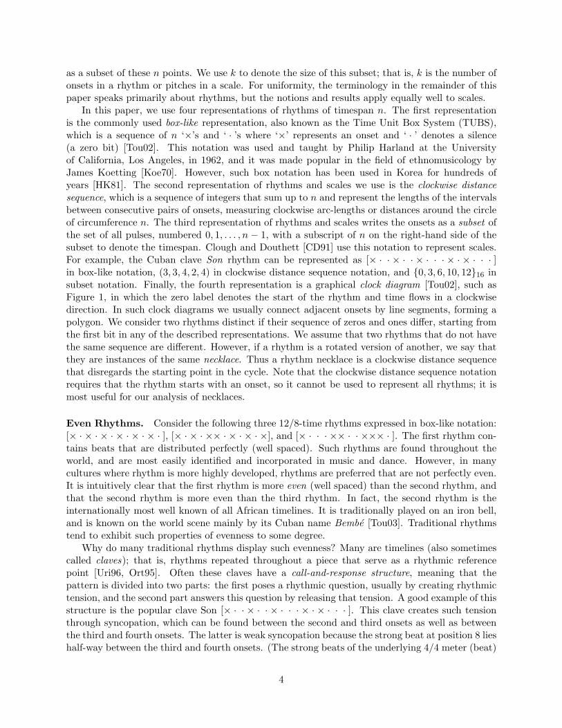
In this paper, we use four representations of rhythms of timespan n. The first representationis the commonly used box-like representation, also known as the Time Unit Box System (TUBS),which is a sequence of n ‘×’s and ‘ · ’s where ‘×’ represents an onset and ‘ · ’ denotes a silence(a zero bit) [Tou02]. This notation was used and taught by Philip Harland at the Universityof California, Los Angeles, in 1962, and it was made popular in the field of ethnomusicology byJames Koetting [Koe70]. However, such box notation has been used in Korea for hundreds ofyears [HK81]. The second representation of rhythms and scales we use is the clockwise distancesequence, which is a sequence of integers that sum up to n and represent the lengths of the intervalsbetween consecutive pairs of onsets, measuring clockwise arc-lengths or distances around the circleof circumference n. The third representation of rhythms and scales writes the onsets as a subset ofthe set of all pulses, numbered 0, 1, . . . , n − 1, with a subscript of n on the right-hand side of thesubset to denote the timespan. Clough and Douthett [CD91] use this notation to represent scales.For example, the Cuban clave Son rhythm can be represented as [× · · × · · × · · · × · × · · · ]in box-like notation, (3, 3, 4, 2, 4) in clockwise distance sequence notation, and 0, 3, 6, 10, 1216 insubset notation. Finally, the fourth representation is a graphical clock diagram [Tou02], such asFigure 1, in which the zero label denotes the start of the rhythm and time flows in a clockwisedirection. In such clock diagrams we usually connect adjacent onsets by line segments, forming apolygon. We consider two rhythms distinct if their sequence of zeros and ones differ, starting fromthe first bit in any of the described representations. We assume that two rhythms that do not havethe same sequence are different. However, if a rhythm is a rotated version of another, we say thatthey are instances of the same necklace. Thus a rhythm necklace is a clockwise distance sequencethat disregards the starting point in the cycle. Note that the clockwise distance sequence notationrequires that the rhythm starts with an onset, so it cannot be used to represent all rhythms; it ismost useful for our analysis of necklaces.
Even Rhythms. Consider the following three 12/8-time rhythms expressed in box-like notation:[× · × · × · × · × · × · ], [× · × · ×× · × · × · ×], and [× · · · ×× · · ××× · ]. The first rhythm con-tains beats that are distributed perfectly (well spaced). Such rhythms are found throughout theworld, and are most easily identified and incorporated in music and dance. However, in manycultures where rhythm is more highly developed, rhythms are preferred that are not perfectly even.It is intuitively clear that the first rhythm is more even (well spaced) than the second rhythm, andthat the second rhythm is more even than the third rhythm. In fact, the second rhythm is theinternationally most well known of all African timelines. It is traditionally played on an iron bell,and is known on the world scene mainly by its Cuban name Bembe [Tou03]. Traditional rhythmstend to exhibit such properties of evenness to some degree.
Why do many traditional rhythms display such evenness? Many are timelines (also sometimescalled claves); that is, rhythms repeated throughout a piece that serve as a rhythmic referencepoint [Uri96, Ort95]. Often these claves have a call-and-response structure, meaning that thepattern is divided into two parts: the first poses a rhythmic question, usually by creating rhythmictension, and the second part answers this question by releasing that tension. A good example of thisstructure is the popular clave Son [× · · × · · × · · · × · × · · · ]. This clave creates such tensionthrough syncopation, which can be found between the second and third onsets as well as betweenthe third and fourth onsets. The latter is weak syncopation because the strong beat at position 8 lieshalf-way between the third and fourth onsets. (The strong beats of the underlying 4/4 meter (beat)
4
occur at positions 0, 4, 8, and 12.) On the other hand, the former syncopation is strong because thestrong beat at position 4 is closer to the second onset than to the third onset [GMRT05]. Clavesplayed with instruments that produce unsustained notes often use syncopation and accentuationto bring about rhythmic tension. Many clave rhythms create syncopation by evenly distributingonsets in contradiction with the pulses of the underlying meter. For example, in the clave Son,the first three onsets are equally spaced at the distance of three sixteenth pulses, which forms acontradiction because 3 does not divide 16. Then, the response of the clave answers with an offbeatonset, followed by an onset on the fourth strong beat of a 4/4 meter, releasing that rhythmictension.
On the other hand, a rhythm that is too even, such as the example [× · × · × · × · × · × · ], isless interesting from a syncopation point of view. Indeed, in the most interesting rhythms withk onsets and timespan n, k and n are relatively prime (have no common divisor larger than 1).This property is natural because the rhythmic contradiction is easier to obtain if the onsets do notcoincide with the strong beats of the meter. Also, we find that many claves have an onset on thelast strong beat of the meter, as does the clave Son. This is a natural way to respond in the call-and-response structure. A different case is that of the Bossa-Nova clave [× · · × · · × · · · × · ·× · · ]. This clave tries to break the feeling of the pulse and, although it is very even, it producesa cycle that perceptually does not coincide with the beginning of the meter.
This prevalence of evenness in world rhythms has led to the study of mathematical measures ofevenness in the new field of mathematical ethnomusicology [Che02, Tou04b, Tou05], where they mayhelp to identify, if not explain, cultural preferences of rhythms in traditional music. Furthermore,evenness in musical chords plays a significant role in the efficacy of voice leading as discussed inthe work of Tymoczko [Tym06, HT07].
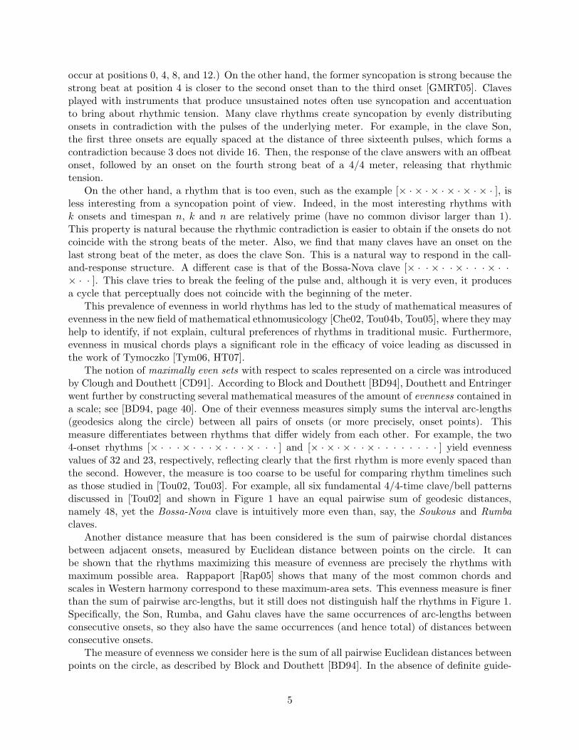
The notion of maximally even sets with respect to scales represented on a circle was introducedby Clough and Douthett [CD91]. According to Block and Douthett [BD94], Douthett and Entringerwent further by constructing several mathematical measures of the amount of evenness contained ina scale; see [BD94, page 40]. One of their evenness measures simply sums the interval arc-lengths(geodesics along the circle) between all pairs of onsets (or more precisely, onset points). Thismeasure differentiates between rhythms that differ widely from each other. For example, the two4-onset rhythms [× · · · × · · · × · · · × · · · ] and [× · × · × · · × · · · · · · · · ] yield evennessvalues of 32 and 23, respectively, reflecting clearly that the first rhythm is more evenly spaced thanthe second. However, the measure is too coarse to be useful for comparing rhythm timelines suchas those studied in [Tou02, Tou03]. For example, all six fundamental 4/4-time clave/bell patternsdiscussed in [Tou02] and shown in Figure 1 have an equal pairwise sum of geodesic distances,namely 48, yet the Bossa-Nova clave is intuitively more even than, say, the Soukous and Rumbaclaves.
Another distance measure that has been considered is the sum of pairwise chordal distancesbetween adjacent onsets, measured by Euclidean distance between points on the circle. It canbe shown that the rhythms maximizing this measure of evenness are precisely the rhythms withmaximum possible area. Rappaport [Rap05] shows that many of the most common chords andscales in Western harmony correspond to these maximum-area sets. This evenness measure is finerthan the sum of pairwise arc-lengths, but it still does not distinguish half the rhythms in Figure 1.Specifically, the Son, Rumba, and Gahu claves have the same occurrences of arc-lengths betweenconsecutive onsets, so they also have the same occurrences (and hence total) of distances betweenconsecutive onsets.
The measure of evenness we consider here is the sum of all pairwise Euclidean distances betweenpoints on the circle, as described by Block and Douthett [BD94]. In the absence of definite guide-
5
13
14
15
7
6
5
4
2
10
89
10
12
11
3 13
14
15
7
6
5
4
2
10
89
10
12
11
3 13
14
15
7
6
5
4
2
10
89
10
3
13
14
15
7
6
5
4
2
10
89
10
12
11
313
14
15
7
6
5
4
2
10
89
10
12
11
313
14
15
7
6
5
4
2
10
89
10
12
11
3
12
11
(a) Shiko (c) Soukous
(e) Bossa−Nova
(b) Son
(d) Rumba (f) Gahu
Figure 1: The six fundamental African and Latin American rhythms which all have equal sum of pairwisegeodesic distances; yet intuitively, the Bossa-Nova rhythm is more “even” than the rest.
lines from music perception psychologists, we adopt this particular method of measuring evennesswithout meaning to imply that it is musically or perceptually important. Later, we generalizeour results to a broad class of measures, of which Euclidean chord lengths is only one. It is worthpointing out that the mathematician Fejes-Toth [T56] showed in 1956 that a configuration of pointson a circle maximizes this sum when the points are the vertices of a regular polygon. This measureis also more discriminating than the others, and is therefore the preferred measure of evenness.For example, this measure distinguishes all of the six rhythms in Figure 1, ranking the Bossa-Novarhythm as the most even, followed by the Son, Rumba, Shiko, Gahu, and Soukous. Intuitively,the rhythms with a larger sum of pairwise chordal distances have more “well spaced” onsets. Itmay seem odd that rhythms “lie” in the one-dimensional musical space, while the evenness of therhythm is measured through chord lengths that “live” in the two-dimensional plane in which thecircle is embedded. However, note that two chords are equal if and only if the two correspondingcircular arcs are equal. Therefore a polygon is regular if and only if all its circular arcs are equal.
In Section 4, we study the mathematical and computational aspects of rhythms that maximizeevenness. We describe three algorithms that generate such rhythms, show that these algorithmsare equivalent, and show that in fact the rhythm of maximum evenness is essentially unique. Theseresults characterize rhythms with maximum evenness. One of the algorithms is the Euclidean-like algorithm from Section 2, proving that the rhythms of maximum evenness are precisely theEuclidean rhythms from that section.
6
7
6
5
4
3
2
10
8910
13
12
11
14
15
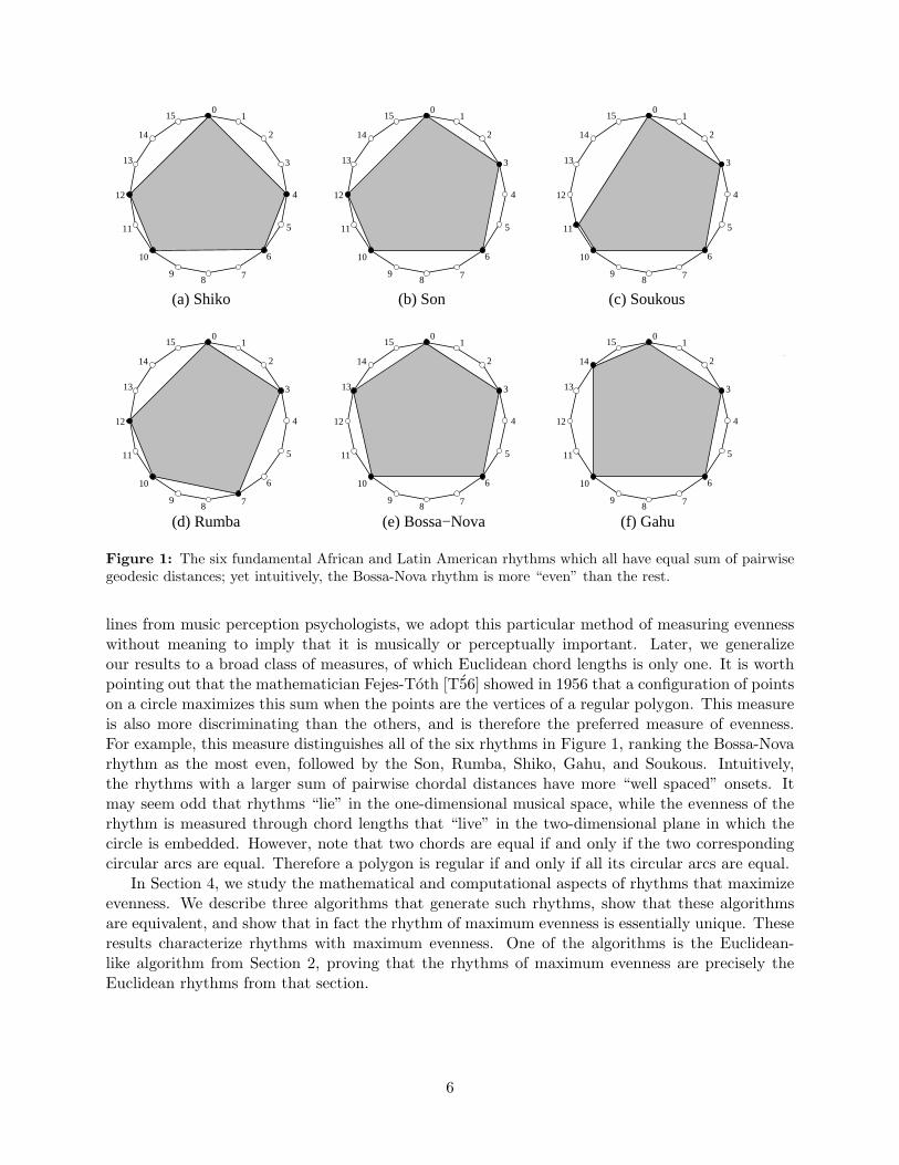
Figure 2: A rhythm with k = 7 onsets and timespan n = 16 that is Winograd-deep and thus Erdos-deep.Distances ordered by multiplicity from 1 to 6 are 2, 7, 4, 1, 6, and 5. The dotted line shows how the rhythmis generated by multiples of m = 5.
Deep Rhythms. Another important property of rhythms and scales that we study in this paperis deepness. Consider a rhythm with k onsets and timespan n, represented as a set of k points on acircle of circumference n. Now measure the arc-length/geodesic distances along the circle betweenall pairs of onsets. A musical scale or rhythm is Winograd-deep if every distance 1, 2, . . . , bn/2c hasa unique number of occurrences (called the multiplicity of the distance). For example, the rhythm[××× · × · ] is Winograd-deep because distance 1 appears twice, distance 2 appears thrice, anddistance 3 appears once.
The notion of deepness in scales was introduced by Winograd in an oft-cited but unpublishedclass project report from 1966 [Win66], disseminated and further developed by the class instructorGamer in 1967 [Gam67a, Gam67b], and considered further in numerous papers and books, such as[CEK99, Joh03]. Equivalently, a scale is Winograd-deep if the number of onsets it has in commonwith each of its cyclic shifts (rotations) is unique. This equivalence is the Common Tone Theorem[Joh03, page 42], originally described by Winograd [Win66] (who in fact uses this definition as hisprimary definition of “deep”). Deepness is one property of the ubiquitous Western diatonic 12-tonemajor scale [× · × · ×× · × · × · ×] [Joh03], and it captures some of the rich structure that perhapsmakes this scale so attractive.
Winograd-deepness translates directly from scales to rhythms. For example, the diatonic majorscale is equivalent to the famous Cuban rhythm Bembe [Pre83, Tou03]. Figure 2 shows a graph-ical example of a Winograd-deep rhythm. However, the notion of Winograd-deepness is ratherrestrictive for rhythms, because it requires half of the pulses in a timespan (rounded to a nearestinteger) to be onsets. In contrast, for example, the popular Bossa-Nova rhythm [× · · × · · × · · ·× · · × · · ] = 0, 3, 6, 10, 1316 illustrated in Figure 1 has only five onsets in a timespan of sixteen.Nonetheless, if we focus on just the distances that appear at least once between two onsets, thenthe multiplicities of occurrence are all unique and form an interval starting at 1: distance 4 occursonce, distance 7 occurs twice, distance 6 occurs thrice, and distance 3 occurs four times.
We therefore define a rhythm (or scale) to be Erdos-deep if it has k onsets and, for everymultiplicity 1, 2, . . . , k−1, there is a nonzero arc-length/geodesic distance determined by the pointson the circle with exactly that multiplicity. The same definition is made by Toussaint [Tou04a].Every Winograd-deep rhythm is also Erdos-deep, so this definition is strictly more general.
To further clarify the difference between Winograd-deep and Erdos-deep rhythms, it is useful toconsider which distances can appear. For a rhythm to be Winograd-deep, all the distances between1 and k − 1 must appear a unique number of times. In contrast, to be an Erdos-deep rhythm,it is only required that each distance that appears must have a unique multiplicity. Thus, the
7
Bossa-Nova rhythm is not Winograd-deep because distances 1, 2 and 5 do not appear.The property of Erdos deepness involves only the distances between points in a set, and is
thus a feature of distance geometry—in this case, in the discrete space of n points equally spacedaround a circle. In 1989, Paul Erdos [Erd89] considered the analogous question in the plane,asking whether there exist n points in the plane (no three on a line and no four on a circle) suchthat, for every i = 1, 2, . . . , n−1, there is a distance determined by these points that occurs exactlyi times. Solutions have been found for n between 2 and 8, but in general the problem remains open.Palasti [Pal89] considered a variant of this problem with further restrictions—no three points forma regular triangle, and no one is equidistant from three others—and solved it for n = 6.
In Section 5, we characterize all rhythms that are Erdos-deep. In particular, we prove that alldeep rhythms, besides one exception, are generated, meaning that the rhythm can be representedas 0,m, 2m, . . . , (k − 1)mn for some integer m, where all arithmetic is modulo n. In the contextof scales, the concept of “generated” was defined by Wooldridge [Woo93] and used by Clough etal. [CEK99]. For example, the rhythm in Figure 2 is generated with m = 5. Our characterizationgeneralizes a similar characterization for Winograd-deep scales proved by Winograd [Win66], andindependently by Clough et al. [CEK99].
In the pitch domain, generated scales are very common. The Pythagorean tuning is a goodexample: all its pitches are generated from the fifth of ratio 3 : 2 modulo the octave. Anotherexample is the equal-tempered scale, which is generated with a half-tone of ratio 12
√2 [Bar04a].
Generated scales are also of interest in the theory of the well-formed scales [Car98].Generated rhythms have an interesting property called shellability. If we remove the “last”
generated onset 14 from the rhythm in Figure 2, the resulting rhythm is still generated, and thisprocess can be repeated until we run out of onsets. In general, every generated rhythm has ashelling in the sense that it is always possible to remove a particular onset and obtain anothergenerated rhythm.
Most African drumming music consists of rhythms operating on three different strata: theunvarying timeline usually provided by one or more bells, one or more rhythmic motifs playedon drums, and an improvised solo (played by the lead drummer) riding on the other rhythmicstructures. Shellings of rhythms are relevant to the improvisation of solo drumming in the contextof such a rhythmic background. The solo improvisation must respect the style and feeling of thepiece which is usually determined by the timeline. One common technique to achieve this effect isto “borrow” notes from the timeline, and to alternate between playing subsets of notes from thetimeline and from other rhythms that interlock with the timeline [Ank97, Aga86]. In the wordsof Kofi Agawu [Aga86], “It takes a fair amount of expertise to create an effective improvisationthat is at the same time stylistically coherent”. The borrowing of notes from the timeline may beregarded as a fulfillment of the requirements of style coherence. Another common method is tomake parsimonious transformations to the timeline or improvise on a rhythm that is functionallyrelated to the timeline [Log84]. Although such an approach does not give the performer wide scopefor free improvisation, it is efficient in certain drumming contexts. In the words of ChristopheWaterman [CW95], “individuals improvise, but only within fairly strict limits, since varying theconstituent parts too much could unravel the overall texture”.
Of course, some subsets of notes of a rhythm may be better choices than others. One mightoften want to select sets of rhythms that share a common property. For example, if a rhythm isdeep, one might want to select subsets of the rhythm that are also deep. Furthermore, a shellingseems a natural way to decrease or increase the density of the notes in an improvisation thatrespects these constraints. For example, in the Bembe bell timeline [× · × · ×× · × · × · ×], whichis deep, one possible shelling is [× · × · ×× · × · × · · ], [× · × · × · · × · × · · ], [× · × · · · · × ·
8
× · · ], [× · × · · · · × · · · · ]. All five rhythms sound good and are stylistically coherent. In factthe shelled rhythms are used in African drum music [Che91]. To our knowledge, shellings have notbeen studied from the musicological point of view. However, they may be useful both for theoreticalanalysis as well as providing formal rules for “improvisation” techniques.
One of the consequences of our characterization that we obtain in Section 5 is that every Erdos-deep rhythm has a shelling. More precisely, it is always possible to remove a particular onsetthat preserves the Erdos-deepness property. Thus this is one method of implementing parsimo-nious transformation of rhythms. Finally, to tie everything together, we show that essentially allEuclidean rhythms (or equivalently, rhythms that maximize evenness) are Erdos-deep.
2 Euclid and Evenness in Various Disciplines
In this section, we first describe Euclid’s classic algorithm for computing the greatest commondivisor of two integers. Then, through an unexpected connection to timing systems in neutronaccelerators, we see how the same type of algorithm can be used as an approach to maximizing“evenness” in a binary string with a specified number of zeroes and ones. This algorithm defines animportant family of rhythms, called Euclidean rhythms, which we show appear throughout worldmusic. Finally, we see how similar ideas have been used in algorithms for drawing digital straightlines and in combinatorial strings called Euclidean strings.
2.1 The Euclidean Algorithm for Greatest Common Divisors
The Euclidean algorithm for computing the greatest common divisor of two integers is one of theoldest known algorithms (circa 300 B.C.). It was first described by Euclid in Proposition 2 ofBook VII of Elements [Euc56, Fra56]. Indeed, Donald Knuth [Knu98] calls this algorithm the“granddaddy of all algorithms, because it is the oldest nontrivial algorithm that has survived tothe present day”.
The idea of the algorithm is simple: repeatedly replace the larger of the two numbers by theirdifference until both are equal. This final number is then the greatest common divisor. For example,consider the numbers 5 and 13. First, 13− 5 = 8; then 8− 5 = 3; next 5− 3 = 2; then 3− 2 = 1;and finally 2 − 1 = 1. Therefore, the greatest common divisor of 5 and 13 is 1; in other words, 5and 13 are relatively prime.
The algorithm can also be described succinctly in a recursive manner as follows [CLRS01]. Letk and n be the input integers with k < n.
Algorithm Euclid(k, n)1. if k = 0 then return n2. else return Euclid(n mod k, k)
Running this algorithm with k = 5 and n = 13, we obtain Euclid(5, 13) = Euclid(3, 5) =Euclid(2, 3) = Euclid(1, 2) = Euclid(0, 1) = 1. Note that this division version of Euclid’salgorithm skips one of the steps (5, 8) made by the original subtraction version.
2.2 Evenness and Timing Systems in Neutron Accelerators
One of our main musical motivations is to find rhythms with a specified timespan and number ofonsets that maximize evenness. Bjorklund [Bjo03b, Bjo03a] was faced with a similar problem of
9
maximizing evenness, but in a different context: the operation of components such as high-voltagepower supplies of spallation neutron source (SNS) accelerators used in nuclear physics. In thissetting, a timing system controls a collection of gates over a time window divided into n equal-length intervals. (In the case of SNS, each interval is 10 seconds.) The timing system can sendsignals to enable a gate during any desired subset of the n intervals. For a given number n of timeintervals, and another given number k < n of signals, the problem is to distribute the pulses asevenly as possible among these n intervals. Bjorklund [Bjo03b] represents this problem as a binarysequence of k ones and n−k zeroes, where each bit represents a time interval and the ones representthe times at which the timing system sends a signal. The problem then reduces to the following:construct a binary sequence of n bits with k ones such that the k ones are distributed as evenly aspossible among the n− k zeroes.
One simple case is when k evenly divides n (without remainder), in which case we should placeones every n/k bits. For example, if n = 16 and k = 4, then the solution is [1000100010001000].This case corresponds to n and k having a common divisor of k. More generally, if the greatestcommon divisor between n and k is g, then we would expect the solution to decompose into grepetitions of a sequence of n/g bits. Intuitively, a string of maximum evenness should have thiskind of symmetry, in which it decomposes into more than one repetition, whenever such symmetry ispossible. This connection to greatest common divisors suggests that a rhythm of maximum evennessmight be computed using an algorithm like Euclid’s. Indeed, Bjorklund’s algorithm closely mimicsthe structure of Euclid’s algorithm, although this connection has never been mentioned before.
We describe Bjorklund’s algorithm by using one of his examples. Consider a sequence withn = 13 and k = 5. Since 13 − 5 = 8, we start by considering a sequence consisting of 5 onesfollowed by 8 zeroes which should be thought of as 13 sequences of one bit each:
[1][1][1][1][1][0][0][0][0][0][0][0][0]
If there is more than one zero the algorithm moves zeroes in stages. We begin by taking zeroesone at a time (from right to left), placing a zero after each one (from left to right), to produce fivesequences of two bits each, with three zeroes remaining:
[10] [10] [10] [10] [10] [0] [0] [0]
Next we distribute the three remaining zeros in a similar manner, by placing a [0] sequence aftereach [10] sequence:
[100] [100] [100] [10] [10]
Now we have three sequences of three bits each, and a remainder of two sequences of two bits each.Therefore we continue in the same manner, by placing a [10] sequence after each [100] sequence:
[10010] [10010] [100]
The process stops when the remainder consists of only one sequence (in this case the sequence[100]), or we run out of zeroes (there is no remainder). The final sequence is thus the concatenationof [10010], [10010], and [100]:
[1001010010100]
We could proceed further in this process by inserting [100] into [10010] [10010]. However,Bjorklund argues that, because the sequence is cyclic, it does not matter (hence his stopping rule).For the same reason, if the initial sequence has a group of ones followed by only one zero, the
10
zero is considered as a remainder consisting of one sequence of one bit, and hence nothing is done.Bjorklund [Bjo03b] shows that the final sequence may be computed from the initial sequence usingO(n) arithmetic operations in the worst case.
A more convenient and visually appealing way to implement this algorithm by hand is to performthe sequence of insertions in a vertical manner as follows. First take five zeroes from the right andplace them under the five ones on the left:
1 1 1 1 1 0 0 00 0 0 0 0
Then move the three remaining zeroes in a similar manner:
1 1 1 1 10 0 0 0 00 0 0
Next place the two remainder columns on the right under the two leftmost columns:
1 1 10 0 00 0 01 10 0
Here the process stops because the remainder consists of only one column. The final sequence isobtained by concatenating the three columns from left to right:
1 0 0 1 0 1 0 0 1 0 1 0 0
Bjorklund’s algorithm applied to a string of n bits consisting of k ones and n − k zeros hasthe same structure as running Euclid(k, n). Indeed, Bjorklund’s algorithm uses the repeatedsubtraction form of division, just as Euclid did in his Elements [Euc56]. It is also well knownthat applying the algorithm Euclid(k, n) to two O(n) bit numbers (binary sequences of length n)causes it to perform O(n) arithmetic operations in the worst case [CLRS01].
2.3 Euclidean Rhythms
The binary sequences generated by Bjorklund’s algorithm, as described in the preceding, maybe considered as one family of rhythms. Furthermore, because Bjorklund’s algorithm is a wayof visualizing the repeated-subtraction version of the Euclidean algorithm, we call these rhythmsEuclidean rhythms. We denote the Euclidean rhythm by E(k, n), where k is the number of ones(onsets) and n (the number of pulses) is the length of the sequence (zeroes plus ones). For ex-ample, E(5, 13) = [1001010010100]. The zero-one notation is not ideal for representing binaryrhythms because it is difficult to visualize the locations of the onsets as well as the duration ofthe inter-onset intervals. In the more iconic box notation, the preceding rhythm is written asE(5, 13) = [× · · × · × · · × · × · · ]. It should be emphasized that Euclidean rhythms are merelythe result of applying Euclid’s algorithm and do not privilege a priori the resulting rhythm overany of its other rotations.
The rhythm E(5, 13) is in fact used in Macedonian music [Aro04], but having a timespan of 13(and defining a measure of length 13), it is rarely found in world music. For contrast, let us considertwo widely used values of k and n; in particular, what is E(3, 8)? Applying Bjorklund’s algorithm
11
1
2
34
5
6
7
0
23
3
1
2
35
6
7
0
4(a) (b)
Figure 3: (a) The Euclidean rhythm E(3, 8) is the Cuban tresillo. (b) The Euclidean rhythm E(5, 8) is theCuban cinquillo.
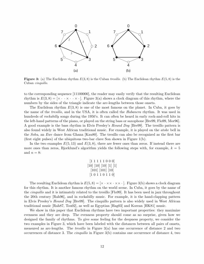
to the corresponding sequence [11100000], the reader may easily verify that the resulting Euclideanrhythm is E(3, 8) = [× · · × · · × · ]. Figure 3(a) shows a clock diagram of this rhythm, where thenumbers by the sides of the triangle indicate the arc-lengths between those onsets.
The Euclidean rhythm E(3, 8) is one of the most famous on the planet. In Cuba, it goes bythe name of the tresillo, and in the USA, it is often called the Habanera rhythm. It was used inhundreds of rockabilly songs during the 1950’s. It can often be heard in early rock-and-roll hits inthe left-hand patterns of the piano, or played on the string bass or saxophone [Bre99, Flo99, Mor96].A good example is the bass rhythm in Elvis Presley’s Hound Dog [Bre99]. The tresillo pattern isalso found widely in West African traditional music. For example, it is played on the atoke bell inthe Sohu, an Ewe dance from Ghana [Kau80]. The tresillo can also be recognized as the first bar(first eight pulses) of the ubiquitous two-bar clave Son shown in Figure 1(b).
In the two examples E(5, 13) and E(3, 8), there are fewer ones than zeros. If instead there aremore ones than zeros, Bjorklund’s algorithm yields the following steps with, for example, k = 5and n = 8:
[1 1 1 1 1 0 0 0][10] [10] [10] [1] [1]
[101] [101] [10][1 0 1 1 0 1 1 0]
The resulting Euclidean rhythm is E(5, 8) = [× · ×× · ×× · ]. Figure 3(b) shows a clock diagramfor this rhythm. It is another famous rhythm on the world scene. In Cuba, it goes by the name ofthe cinquillo and it is intimately related to the tresillo [Flo99]. It has been used in jazz throughoutthe 20th century [Rah96], and in rockabilly music. For example, it is the hand-clapping patternin Elvis Presley’s Hound Dog [Bre99]. The cinquillo pattern is also widely used in West Africantraditional music [Rah87, Tou02], as well as Egyptian [Hag03] and Korean [HK81] music.
We show in this paper that Euclidean rhythms have two important properties: they maximizeevenness and they are deep. The evenness property should come as no surprise, given how wedesigned the family of rhythms. To give some feeling for the deepness property, we consider thetwo examples in Figure 3, which have been labeled with the distances between all pairs of onsets,measured as arc-lengths. The tresillo in Figure 3(a) has one occurrence of distance 2 and twooccurrences of distance 3. The cinquillo in Figure 3(b) contains one occurrence of distance 4, two
12
1
2
3
4
56
7
8
9
10
110 1
2
3
4
56
7
8
9
10
110
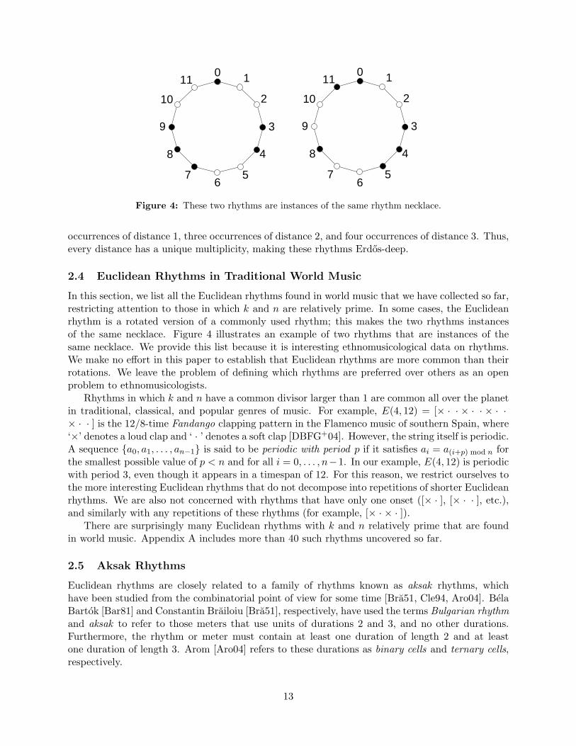
Figure 4: These two rhythms are instances of the same rhythm necklace.
occurrences of distance 1, three occurrences of distance 2, and four occurrences of distance 3. Thus,every distance has a unique multiplicity, making these rhythms Erdos-deep.
2.4 Euclidean Rhythms in Traditional World Music
In this section, we list all the Euclidean rhythms found in world music that we have collected so far,restricting attention to those in which k and n are relatively prime. In some cases, the Euclideanrhythm is a rotated version of a commonly used rhythm; this makes the two rhythms instancesof the same necklace. Figure 4 illustrates an example of two rhythms that are instances of thesame necklace. We provide this list because it is interesting ethnomusicological data on rhythms.We make no effort in this paper to establish that Euclidean rhythms are more common than theirrotations. We leave the problem of defining which rhythms are preferred over others as an openproblem to ethnomusicologists.
Rhythms in which k and n have a common divisor larger than 1 are common all over the planetin traditional, classical, and popular genres of music. For example, E(4, 12) = [× · · × · · × · ·× · · ] is the 12/8-time Fandango clapping pattern in the Flamenco music of southern Spain, where‘×’ denotes a loud clap and ‘ · ’ denotes a soft clap [DBFG+04]. However, the string itself is periodic.A sequence a0, a1, . . . , an−1 is said to be periodic with period p if it satisfies ai = a(i+p) mod n forthe smallest possible value of p < n and for all i = 0, . . . , n−1. In our example, E(4, 12) is periodicwith period 3, even though it appears in a timespan of 12. For this reason, we restrict ourselves tothe more interesting Euclidean rhythms that do not decompose into repetitions of shorter Euclideanrhythms. We are also not concerned with rhythms that have only one onset ([× · ], [× · · ], etc.),and similarly with any repetitions of these rhythms (for example, [× · × · ]).
There are surprisingly many Euclidean rhythms with k and n relatively prime that are foundin world music. Appendix A includes more than 40 such rhythms uncovered so far.
2.5 Aksak Rhythms
Euclidean rhythms are closely related to a family of rhythms known as aksak rhythms, whichhave been studied from the combinatorial point of view for some time [Bra51, Cle94, Aro04]. BelaBartok [Bar81] and Constantin Brailoiu [Bra51], respectively, have used the terms Bulgarian rhythmand aksak to refer to those meters that use units of durations 2 and 3, and no other durations.Furthermore, the rhythm or meter must contain at least one duration of length 2 and at leastone duration of length 3. Arom [Aro04] refers to these durations as binary cells and ternary cells,respectively.
13
Arom [Aro04] generated an inventory of all the theoretically possible aksak rhythms for valuesof n ranging from 5 to 29, as well as a list of those that are actually used in traditional worldmusic. He also proposed a classification of these rhythms into several classes, based on structuraland numeric properties. Three of his classes are considered here:
1. An aksak rhythm is authentic if n is prime.
2. An aksak rhythm is quasi-aksak if n is odd but not prime.
3. An aksak rhythm is pseudo-aksak if n is even.
A quick perusal of the Euclidean rhythms listed in Appendix A reveals that aksak rhythms arewell represented. Indeed, all three of Arom’s classes (authentic, quasi-aksak, and pseudo-aksak)make their appearance. There is a simple characterization of those Euclidean rhythms that areaksak. From the iterative subtraction algorithm of Bjorklund it follows that if n = 2k all cells arebinary (duration 2). Similarly, if n = 3k all cells are ternary (duration 3). Therefore, to ensure thatthe Euclidean rhythm contains both binary and ternary cells, and no other durations, it followsthat n must be between 2k and 3k.
Of course, not all aksak rhythms are Euclidean. Consider the Bulgarian rhythm with intervalsequence (3322) [Aro04], which is also the metric pattern of Indian Lady by Don Ellis [Kei91]. Herek = 4 and n = 10, and E(4, 10) = [× · · × · × · · × · ] or (3232), a periodic rhythm.
The following Euclidean rhythms are authentic aksak :
E(2, 5) = [× · × · · ] = (23) (classical music, jazz, Greece, Macedonia, Namibia, Persia, Rwanda).E(3, 7) = [× · × · × · · ] = (223) (Bulgaria, Greece, Sudan, Turkestan).E(4, 11) = [× · · × · · × · · × · ] = (3332) (Southern India rhythm), (Serbian necklace).E(5, 11) = [× · × · × · × · × · · ] = (22223) (classical music, Bulgaria, Northern India, Serbia).E(5, 13) = [× · · × · × · · × · × · · ] = (32323) (Macedonia).E(6, 13) = [× · × · × · × · × · × · · ] = (222223) (Macedonia).E(7, 17) = [× · · × · × · · × · × · · × · × · ] = (3232322) (Macedonian necklace).E(8, 17) = [× · × · × · × · × · × · × · × · · ] = (22222223) (Bulgaria).E(8, 19) = [× · · × · × · × · · × · × · × · · × · ] = (32232232) (Bulgaria).E(9, 23) = [× · · × · × · · × · × · · × · × · · × · × · · ] = (323232323) (Bulgaria).
The following Euclidean rhythms are quasi-aksak :
E(4, 9) = [× · × · × · × · · ] = (2223) (Greece, Macedonia, Turkey, Zaıre).E(7, 15) = [× · × · × · × · × · × · × · · ] = (2222223) (Bulgarian necklace).
The following Euclidean rhythms are pseudo-aksak :
E(3, 8) = [× · · × · · × · ] = (332) (Central Africa, Greece, India, Latin America, West Africa, Su-dan).E(5, 12) = [× · · × · × · · × · × · ] = (32322) (Macedonia, South Africa).E(7, 16) = [× · · × · × · × · · × · × · × · ] = (3223222) (Brazilian, Macedonian, West African neck-laces).E(7, 18) = [× · · × · × · · × · × · · × · × · · ] = (3232323) (Bulgaria).E(9, 22) = [× · · × · × · · × · × · · × · × · · × · × · ] = (323232322) (Bulgarian necklace).E(11, 24) = [× · · × · × · × · × · × · · × · × · × · × · × · ] = (32222322222) (Central African and Bul-garian necklaces).E(15, 34) = [× · · × · × · × · × · · × · × · × · × · · × · × · × · × · · × · × · ] = (322232223222322) (Bul-garian necklace).
14
0
1
2
3
4
5
0 161284p
q
Figure 5: The shaded pixels form a digital straight line determined by the points p and q.
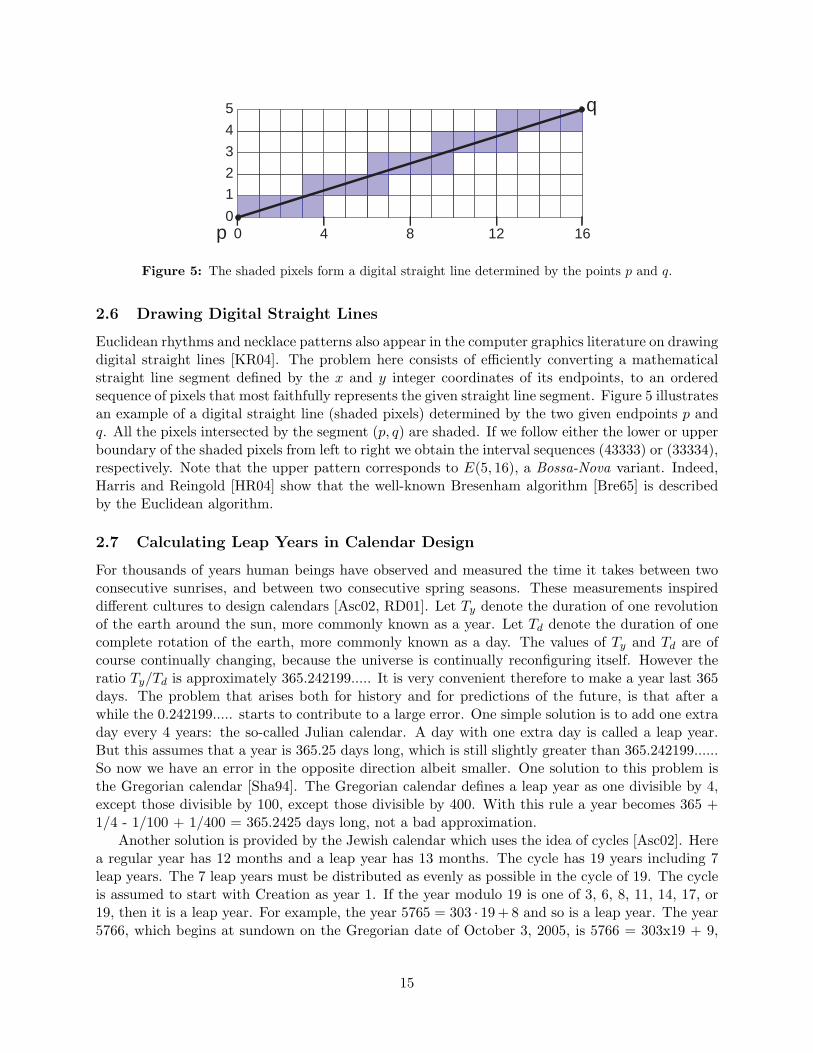
2.6 Drawing Digital Straight Lines
Euclidean rhythms and necklace patterns also appear in the computer graphics literature on drawingdigital straight lines [KR04]. The problem here consists of efficiently converting a mathematicalstraight line segment defined by the x and y integer coordinates of its endpoints, to an orderedsequence of pixels that most faithfully represents the given straight line segment. Figure 5 illustratesan example of a digital straight line (shaded pixels) determined by the two given endpoints p andq. All the pixels intersected by the segment (p, q) are shaded. If we follow either the lower or upperboundary of the shaded pixels from left to right we obtain the interval sequences (43333) or (33334),respectively. Note that the upper pattern corresponds to E(5, 16), a Bossa-Nova variant. Indeed,Harris and Reingold [HR04] show that the well-known Bresenham algorithm [Bre65] is describedby the Euclidean algorithm.
2.7 Calculating Leap Years in Calendar Design
For thousands of years human beings have observed and measured the time it takes between twoconsecutive sunrises, and between two consecutive spring seasons. These measurements inspireddifferent cultures to design calendars [Asc02, RD01]. Let Ty denote the duration of one revolutionof the earth around the sun, more commonly known as a year. Let Td denote the duration of onecomplete rotation of the earth, more commonly known as a day. The values of Ty and Td are ofcourse continually changing, because the universe is continually reconfiguring itself. However theratio Ty/Td is approximately 365.242199..... It is very convenient therefore to make a year last 365days. The problem that arises both for history and for predictions of the future, is that after awhile the 0.242199..... starts to contribute to a large error. One simple solution is to add one extraday every 4 years: the so-called Julian calendar. A day with one extra day is called a leap year.But this assumes that a year is 365.25 days long, which is still slightly greater than 365.242199......So now we have an error in the opposite direction albeit smaller. One solution to this problem isthe Gregorian calendar [Sha94]. The Gregorian calendar defines a leap year as one divisible by 4,except those divisible by 100, except those divisible by 400. With this rule a year becomes 365 +1/4 - 1/100 + 1/400 = 365.2425 days long, not a bad approximation.
Another solution is provided by the Jewish calendar which uses the idea of cycles [Asc02]. Herea regular year has 12 months and a leap year has 13 months. The cycle has 19 years including 7leap years. The 7 leap years must be distributed as evenly as possible in the cycle of 19. The cycleis assumed to start with Creation as year 1. If the year modulo 19 is one of 3, 6, 8, 11, 14, 17, or19, then it is a leap year. For example, the year 5765 = 303 · 19 + 8 and so is a leap year. The year5766, which begins at sundown on the Gregorian date of October 3, 2005, is 5766 = 303x19 + 9,
15
1
2
3
4
56
7
8
9
10
110
1
2
3
4
56
7
8
9
10
110
1
2
3
4
56
7
8
9
10
110
(a) (b) (c)
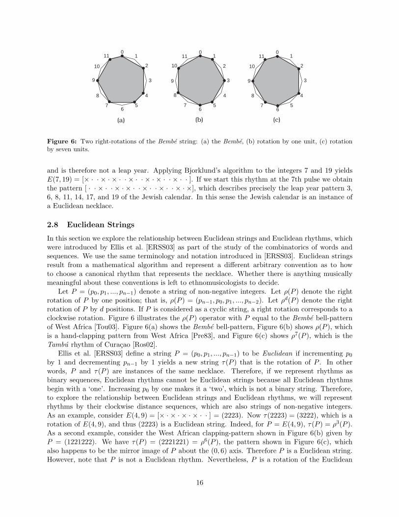
Figure 6: Two right-rotations of the Bembe string: (a) the Bembe, (b) rotation by one unit, (c) rotationby seven units.
and is therefore not a leap year. Applying Bjorklund’s algorithm to the integers 7 and 19 yieldsE(7, 19) = [× · · × · × · · × · · × · × · · × · · ]. If we start this rhythm at the 7th pulse we obtainthe pattern [ · · × · · × · × · · × · · × · · × · ×], which describes precisely the leap year pattern 3,6, 8, 11, 14, 17, and 19 of the Jewish calendar. In this sense the Jewish calendar is an instance ofa Euclidean necklace.
2.8 Euclidean Strings
In this section we explore the relationship between Euclidean strings and Euclidean rhythms, whichwere introduced by Ellis et al. [ERSS03] as part of the study of the combinatorics of words andsequences. We use the same terminology and notation introduced in [ERSS03]. Euclidean stringsresult from a mathematical algorithm and represent a different arbitrary convention as to howto choose a canonical rhythm that represents the necklace. Whether there is anything musicallymeaningful about these conventions is left to ethnomusicologists to decide.
Let P = (p0, p1, ..., pn−1) denote a string of non-negative integers. Let ρ(P ) denote the rightrotation of P by one position; that is, ρ(P ) = (pn−1, p0, p1, ..., pn−2). Let ρd(P ) denote the rightrotation of P by d positions. If P is considered as a cyclic string, a right rotation corresponds to aclockwise rotation. Figure 6 illustrates the ρ(P ) operator with P equal to the Bembe bell-patternof West Africa [Tou03]. Figure 6(a) shows the Bembe bell-pattern, Figure 6(b) shows ρ(P ), whichis a hand-clapping pattern from West Africa [Pre83], and Figure 6(c) shows ρ7(P ), which is theTambu rhythm of Curacao [Ros02].
Ellis et al. [ERSS03] define a string P = (p0, p1, ..., pn−1) to be Euclidean if incrementing p0
by 1 and decrementing pn−1 by 1 yields a new string τ(P ) that is the rotation of P . In otherwords, P and τ(P ) are instances of the same necklace. Therefore, if we represent rhythms asbinary sequences, Euclidean rhythms cannot be Euclidean strings because all Euclidean rhythmsbegin with a ‘one’. Increasing p0 by one makes it a ‘two’, which is not a binary string. Therefore,to explore the relationship between Euclidean strings and Euclidean rhythms, we will representrhythms by their clockwise distance sequences, which are also strings of non-negative integers.As an example, consider E(4, 9) = [× · × · × · × · · ] = (2223). Now τ(2223) = (3222), which is arotation of E(4, 9), and thus (2223) is a Euclidean string. Indeed, for P = E(4, 9), τ(P ) = ρ3(P ).As a second example, consider the West African clapping-pattern shown in Figure 6(b) given byP = (1221222). We have τ(P ) = (2221221) = ρ6(P ), the pattern shown in Figure 6(c), whichalso happens to be the mirror image of P about the (0, 6) axis. Therefore P is a Euclidean string.However, note that P is not a Euclidean rhythm. Nevertheless, P is a rotation of the Euclidean
16
rhythm E(7, 12) = (2122122).Ellis et al. [ERSS03] have many beautiful results about Euclidean strings. They show that
Euclidean strings exist if, and only if, n and p0 +p1 + ...+pn−1 are relatively prime, and that whenthey exist they are unique. They also show how to construct Euclidean strings using an algorithmthat has the same structure as the Euclidean algorithm. In addition they relate Euclidean stringsto many other families of sequences studied in the combinatorics of words [AS02, Lot02].
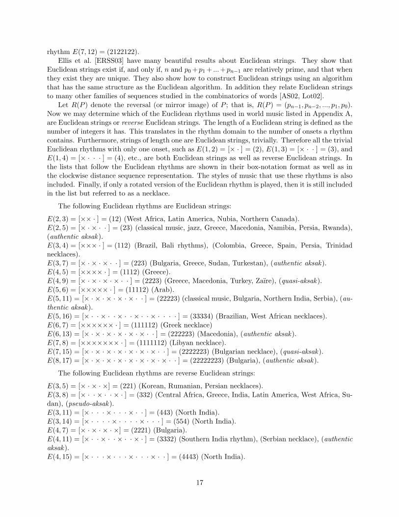
Let R(P ) denote the reversal (or mirror image) of P ; that is, R(P ) = (pn−1, pn−2, ..., p1, p0).Now we may determine which of the Euclidean rhythms used in world music listed in Appendix A,are Euclidean strings or reverse Euclidean strings. The length of a Euclidean string is defined as thenumber of integers it has. This translates in the rhythm domain to the number of onsets a rhythmcontains. Furthermore, strings of length one are Euclidean strings, trivially. Therefore all the trivialEuclidean rhythms with only one onset, such as E(1, 2) = [× · ] = (2), E(1, 3) = [× · · ] = (3), andE(1, 4) = [× · · · ] = (4), etc., are both Euclidean strings as well as reverse Euclidean strings. Inthe lists that follow the Euclidean rhythms are shown in their box-notation format as well as inthe clockwise distance sequence representation. The styles of music that use these rhythms is alsoincluded. Finally, if only a rotated version of the Euclidean rhythm is played, then it is still includedin the list but referred to as a necklace.
The following Euclidean rhythms are Euclidean strings:
E(2, 3) = [×× · ] = (12) (West Africa, Latin America, Nubia, Northern Canada).E(2, 5) = [× · × · · ] = (23) (classical music, jazz, Greece, Macedonia, Namibia, Persia, Rwanda),(authentic aksak).E(3, 4) = [××× · ] = (112) (Brazil, Bali rhythms), (Colombia, Greece, Spain, Persia, Trinidadnecklaces).E(3, 7) = [× · × · × · · ] = (223) (Bulgaria, Greece, Sudan, Turkestan), (authentic aksak).E(4, 5) = [×××× · ] = (1112) (Greece).E(4, 9) = [× · × · × · × · · ] = (2223) (Greece, Macedonia, Turkey, Zaıre), (quasi-aksak).E(5, 6) = [××××× · ] = (11112) (Arab).E(5, 11) = [× · × · × · × · × · · ] = (22223) (classical music, Bulgaria, Northern India, Serbia), (au-thentic aksak).E(5, 16) = [× · · × · · × · · × · · × · · · · ] = (33334) (Brazilian, West African necklaces).E(6, 7) = [×××××× · ] = (111112) (Greek necklace)E(6, 13) = [× · × · × · × · × · × · · ] = (222223) (Macedonia), (authentic aksak).E(7, 8) = [××××××× · ] = (1111112) (Libyan necklace).E(7, 15) = [× · × · × · × · × · × · × · · ] = (2222223) (Bulgarian necklace), (quasi-aksak).E(8, 17) = [× · × · × · × · × · × · × · × · · ] = (22222223) (Bulgaria), (authentic aksak).
The following Euclidean rhythms are reverse Euclidean strings:
E(3, 5) = [× · × · ×] = (221) (Korean, Rumanian, Persian necklaces).E(3, 8) = [× · · × · · × · ] = (332) (Central Africa, Greece, India, Latin America, West Africa, Su-dan), (pseudo-aksak).E(3, 11) = [× · · · × · · · × · · ] = (443) (North India).E(3, 14) = [× · · · · × · · · · × · · · ] = (554) (North India).E(4, 7) = [× · × · × · ×] = (2221) (Bulgaria).E(4, 11) = [× · · × · · × · · × · ] = (3332) (Southern India rhythm), (Serbian necklace), (authenticaksak).E(4, 15) = [× · · · × · · · × · · · × · · ] = (4443) (North India).
17
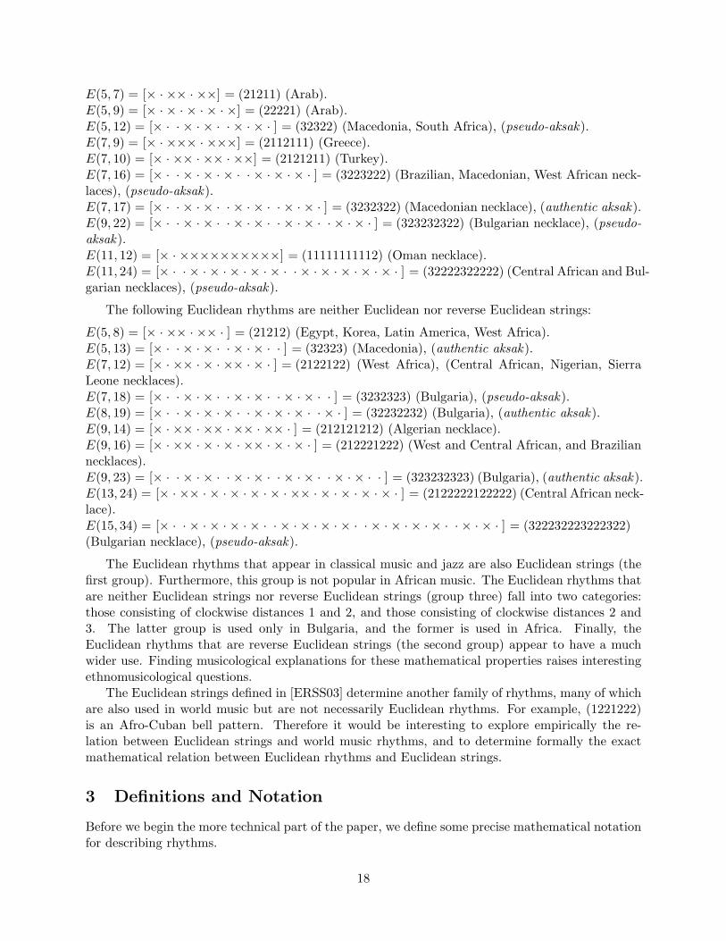
E(5, 7) = [× · ×× · ××] = (21211) (Arab).E(5, 9) = [× · × · × · × · ×] = (22221) (Arab).E(5, 12) = [× · · × · × · · × · × · ] = (32322) (Macedonia, South Africa), (pseudo-aksak).E(7, 9) = [× · ××× · ×××] = (2112111) (Greece).E(7, 10) = [× · ×× · ×× · ××] = (2121211) (Turkey).E(7, 16) = [× · · × · × · × · · × · × · × · ] = (3223222) (Brazilian, Macedonian, West African neck-laces), (pseudo-aksak).E(7, 17) = [× · · × · × · · × · × · · × · × · ] = (3232322) (Macedonian necklace), (authentic aksak).E(9, 22) = [× · · × · × · · × · × · · × · × · · × · × · ] = (323232322) (Bulgarian necklace), (pseudo-aksak).E(11, 12) = [× · ××××××××××] = (11111111112) (Oman necklace).E(11, 24) = [× · · × · × · × · × · × · · × · × · × · × · × · ] = (32222322222) (Central African and Bul-garian necklaces), (pseudo-aksak).
The following Euclidean rhythms are neither Euclidean nor reverse Euclidean strings:
E(5, 8) = [× · ×× · ×× · ] = (21212) (Egypt, Korea, Latin America, West Africa).E(5, 13) = [× · · × · × · · × · × · · ] = (32323) (Macedonia), (authentic aksak).E(7, 12) = [× · ×× · × · ×× · × · ] = (2122122) (West Africa), (Central African, Nigerian, SierraLeone necklaces).E(7, 18) = [× · · × · × · · × · × · · × · × · · ] = (3232323) (Bulgaria), (pseudo-aksak).E(8, 19) = [× · · × · × · × · · × · × · × · · × · ] = (32232232) (Bulgaria), (authentic aksak).E(9, 14) = [× · ×× · ×× · ×× · ×× · ] = (212121212) (Algerian necklace).E(9, 16) = [× · ×× · × · × · ×× · × · × · ] = (212221222) (West and Central African, and Braziliannecklaces).E(9, 23) = [× · · × · × · · × · × · · × · × · · × · × · · ] = (323232323) (Bulgaria), (authentic aksak).E(13, 24) = [× · ×× · × · × · × · × · ×× · × · × · × · × · ] = (2122222122222) (Central African neck-lace).E(15, 34) = [× · · × · × · × · × · · × · × · × · × · · × · × · × · × · · × · × · ] = (322232223222322)(Bulgarian necklace), (pseudo-aksak).
The Euclidean rhythms that appear in classical music and jazz are also Euclidean strings (thefirst group). Furthermore, this group is not popular in African music. The Euclidean rhythms thatare neither Euclidean strings nor reverse Euclidean strings (group three) fall into two categories:those consisting of clockwise distances 1 and 2, and those consisting of clockwise distances 2 and3. The latter group is used only in Bulgaria, and the former is used in Africa. Finally, theEuclidean rhythms that are reverse Euclidean strings (the second group) appear to have a muchwider use. Finding musicological explanations for these mathematical properties raises interestingethnomusicological questions.
The Euclidean strings defined in [ERSS03] determine another family of rhythms, many of whichare also used in world music but are not necessarily Euclidean rhythms. For example, (1221222)is an Afro-Cuban bell pattern. Therefore it would be interesting to explore empirically the re-lation between Euclidean strings and world music rhythms, and to determine formally the exactmathematical relation between Euclidean rhythms and Euclidean strings.
3 Definitions and Notation
Before we begin the more technical part of the paper, we define some precise mathematical notationfor describing rhythms.
18
Let Z+ denote the set of positive integers. For k, n ∈ Z+, let gcd(k, n) denote the greatestcommon divisor of k and n. If gcd(k, n) = 1, we call k and n relatively prime. For integers a < b,let [a, b] = a, a + 1, a + 2, . . . , b.
Let C be a circle in the plane, and consider any two points x, y on C. The chordal distancebetween x and y, denoted by d(x, y), is the length of the line segment xy; that is, d(x, y) is theEuclidean distance between x and y. The clockwise distance from x to y, or of the ordered pair(x, y), is the length of the clockwise arc of C from x to y, and is denoted by
ñd(x, y). Finally, the
geodesic distance between x and y, denoted byòd(x, y), is the length of the shortest arc of C between
x and y; that is,òd(x, y) = minñd(x, y),
ñd(y, x).
A rhythm of timespan n is a subset of 0, 1, . . . , n − 1, representing the set of pulses that areonsets in each repetition. For clarity, we write the timespan n as a subscript after the subset: . . . n.Geometrically, if we locate n equally spaced points clockwise around a circle Cn of circumference n,then we can view a rhythm of timespan n as a subset of these n points. We consider an element ofCn to simultaneously be a point on the circle and an integer in 0, 1, . . . , n− 1.
The rotation of a rhythm R of timespan n by an integer ∆ ≥ 0 is the rhythm (i + ∆) mod n :i ∈ Rn of the same timespan n. The scaling of a rhythm R of timespan n by an integer α ≥ 1 isthe rhythm αi : i ∈ Rαn of timespan αn.
Let R = r0, r1, . . . , rk−1n be a rhythm of timespan n with k onsets sorted in clockwise order.Throughout this paper, an onset ri will mean (ri mod k) mod n. Observe that the clockwise distanceñd(ri, rj) = (rj − ri) mod n. This is the number of points on Cn that are contained in the clockwisearc (ri, rj ] and is also known as the chromatic length [CD91].
The geodesic distance multiset of a rhythm R is the multiset of all nonzero pairwise geodesicdistances; that is, it is the multiset òd(ri, rj) : ri, rj ∈ R, ri 6= rj. The geodesic distance multisethas cardinality
(k2
). The multiplicity of a distance d is the number of occurrences of d in the geodesic
distance multiset.A rhythm is Erdos-deep if it has (exactly) one distance of multiplicity i, for each i ∈ [1, k − 1].
Note that these multiplicities sum to∑k−1
i=1 i =(k2
), which is the cardinality of the geodesic distance
multiset, and hence these distances are all the distances in the rhythm. Every geodesic distance isbetween 0 and bn/2c. A rhythm is Winograd-deep if every two distances from 1, 2, . . . , bn2 c havedifferent multiplicity.
A shelling of an Erdos-deep rhythm R is an ordering s1, s2, . . . , sk of the onsets in R such thatR − s1, s2, . . . , si is an Erdos-deep rhythm for i = 0, 1, . . . , k. (Every rhythm with at most twoonsets is Erdos-deep.)
The evenness of rhythm R is the sum of all inter-onset chordal distances in R; that is,∑0≤i<j≤k−1
d(ri, rj).
The clockwise distance sequence of R is the circular sequence (d0, d1, . . . , dk−1) where di =ñd(ri, ri+1) for all i ∈ [0, k − 1]. Observe that each di ∈ Z+ and
∑i di = n.
Observation 1. There is a one-to-one relationship between rhythms with k onsets and timespan nand circular sequences (d0, d1, . . . , dk−1) where each di ∈ Z+ and
∑i di = n.
4 Even Rhythms
In this section we first describe three algorithms that generate even rhythms. We then characterizerhythms with maximum evenness and show that, for given numbers of pulses and onsets, the three
19
described algorithms generate the unique rhythm with maximum evenness. As mentioned in theintroduction, the measure of evenness considered here is the pairwise sum of chordal distances.
The even rhythms characterized in this section were studied by Clough and Meyerson [CM85,CM86] for the case where the numbers of pulses and onsets are relatively prime. This was sub-sequently expanded upon by Clough and Douthett [CD91]. We revisit these results and providean additional connection to rhythms (and scales) that are obtained from the Euclidean algorithm.Most of these results are stated in [CD91]. However our proofs are new, and in many cases aremuch more streamlined.
4.1 Characterization
We first present three algorithms for computing a rhythm with k onsets, timespan n, for any k ≤ n,that possess large evenness.
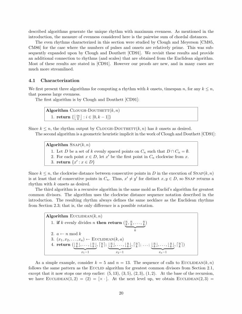
The first algorithm is by Clough and Douthett [CD91]:
Algorithm Clough-Douthett(k, n)1. return
⌊ink
⌋: i ∈ [0, k − 1]
Since k ≤ n, the rhythm output by Clough-Douthett(k, n) has k onsets as desired.The second algorithm is a geometric heuristic implicit in the work of Clough and Douthett [CD91]:
Algorithm Snap(k, n)1. Let D be a set of k evenly spaced points on Cn such that D ∩ Cn = ∅.2. For each point x ∈ D, let x′ be the first point in Cn clockwise from x.3. return x′ : x ∈ D
Since k ≤ n, the clockwise distance between consecutive points in D in the execution of Snap(k, n)is at least that of consecutive points in Cn. Thus, x′ 6= y′ for distinct x, y ∈ D, so Snap returns arhythm with k onsets as desired.
The third algorithm is a recursive algorithm in the same mold as Euclid’s algorithm for greatestcommon divisors. The algorithm uses the clockwise distance sequence notation described in theintroduction. The resulting rhythm always defines the same necklace as the Euclidean rhythmsfrom Section 2.3; that is, the only difference is a possible rotation.
Algorithm Euclidean(k, n)1. if k evenly divides n then return (n
k , nk , . . . , n
k︸ ︷︷ ︸k
)
2. a← n mod k3. (x1, x2, . . . , xa)← Euclidean(k, a)4. return (bnk c, . . . , b
nk c︸ ︷︷ ︸
x1−1
, dnk e; bnk c, . . . , b
nk c︸ ︷︷ ︸
x2−1
, dnk e; . . . ; bnk c, . . . , bnk c︸ ︷︷ ︸
xa−1
, dnk e)
As a simple example, consider k = 5 and n = 13. The sequence of calls to Euclidean(k, n)follows the same pattern as the Euclid algorithm for greatest common divisors from Section 2.1,except that it now stops one step earlier: (5, 13), (3, 5), (2, 3), (1, 2). At the base of the recursion,we have Euclidean(1, 2) = (2) = [× · ]. At the next level up, we obtain Euclidean(2, 3) =
20
(1, 2) = [×× · ]. Next we obtain Euclidean(3, 5) = (2; 1, 2) = [× · ×× · ]. Finally, we obtain Eu-clidean(5, 13) = (2, 3; 3; 2, 3) = [× · × · · × · · × · × · · ]. (For comparison, the Euclidean rhythmfrom Section 2.2 is E(5, 13) = (2, 3, 2, 3, 3), a rotation by 5.)
We now show that algorithm Euclidean(k, n) outputs a circular sequence of k integers thatsum to n (which is thus the clockwise distance sequence of a rhythm with k onsets and timespan n).We proceed by induction on k. If k evenly divides n, then the claim clearly holds. Otherwise a(= n mod k) > 0, and by induction
∑ai=1 xi = k. Thus the sequence that is output has k terms
and sums to
a⌈n
k
⌉+
⌊n
k
⌋ a∑i=1
(xi − 1) = a⌈n
k
⌉+ (k − a)
⌊n
k
⌋= a
(1 +
⌊n
k
⌋)+ (k − a)
⌊n
k
⌋= a + k
⌊n
k
⌋= n .
The following theorem is one of the main contributions of this paper.
Theorem 4.1. Let n ≥ k ≥ 2 be integers. The following are equivalent for a rhythm R =r0, r1, . . . , rk−1n with k onsets and timespan n:
(A) R has maximum evenness (sum of pairwise inter-onset chordal distances);
(B) R is a rotation of the Clough-Douthett(k, n) rhythm;
(C) R is a rotation of the Snap(k, n) rhythm;
(D) R is a rotation of the Euclidean(k, n) rhythm; and
(?) for all ` ∈ [1, k − 1] and i ∈ [0, k − 1], the ordered pair (ri, ri+`) has clockwise distanceñd(ri, ri+`) ∈ b `n
k c, d`nk e.
Moreover, up to a rotation, there is a unique rhythm that satisfies these conditions.
Note that the evenness of a rhythm equals the evenness of the same rhythm played backwards.Thus, if R is the unique rhythm with maximum evenness, then R is the same rhythm as R playedbackwards (up to a rotation).
The proof of Theorem 4.1 proceeds as follows. In Section 4.2 we prove that each of the threealgorithms produces a rhythm that satisfies property (?). Then in Section 4.3 we prove that there isa unique rhythm that satisfies property (?). Thus the three algorithms produce the same rhythm,up to rotation. Finally in Section 4.4 we prove that the unique rhythm that satisfies property (?)maximizes evenness.
4.2 Properties of the Algorithms
We now prove that each of the algorithms has property (?). Clough and Douthett [CD91] provedthe following.
21
Proof (B) ⇒ (?). Say R = r0, r1, . . . , rk−1n is the Clough-Douthett(k, n) rhythm. Consideran ordered pair (ri, ri+`) of onsets in R. Let pi = in mod k and let p` = `n mod k. By symmetrywe can suppose that ri ≤ r(i+`) mod k. Then the clockwise distance
ñd(ri, ri+`) is⌊
(i + `)nk
⌋−
⌊in
k
⌋=
⌊in
k
⌋+
⌊`n
k
⌋+
⌊pi + p`
k
⌋−
⌊in
k
⌋=
⌊`n
k
⌋+
⌊pi + p`
k
⌋,
which is⌊
`nk
⌋or
⌈`nk
⌉, because
⌊pi+p`k
⌋∈ 0, 1.
A similar proof shows that the rhythm ⌈
ink
⌉: i ∈ [0, k − 1] satisfies property (?). Observe
that (?) is equivalent to the following property.
(??) If (d0, d1, . . . , dk−1) is the clockwise distance sequence of R, then for all ` ∈ [1, k−1], the sumof any ` consecutive elements in (d0, d1, . . . , dk−1) equals d `nk e or b `nk c.
Proof (C) ⇒ (??). Let (d0, d1, . . . , dk−1) be the clockwise distance sequence of the rhythm deter-mined by Snap(k, n). For the sake of contradiction, suppose that for some ` ∈ [1, k − 1], the sumof ` consecutive elements in (d0, d1, . . . , dk−1) is greater than d `nk e. The case in which the sum isless than b `nk c is analogous. We can assume that these ` consecutive elements are (d0, d1, . . . , d`−1).Using the notation defined in the statement of the algorithm, let x0, x1, . . . , x` be the points in Dsuch that
ñd(x′i, x
′i+1) = di for all i ∈ [0, `− 1]. Thus
ñd(x′1, x
′`+1) ≥ d
`nk e+ 1. Now
ñd(x`+1, x
′`+1) < 1.
Thusñd(x′1, x`+1) > d `nk e ≥
`nk , which implies that
ñd(x1, x`+1) > `n
k . This contradicts the fact thatthe points in D were evenly spaced around Cn in the first step of the algorithm.
Proof (D) ⇒ (??). We proceed by induction on k. Let R =Euclidean(k, n). If k evenly divides n,then R = (n
k , nk , . . . , n
k ), which satisfies (D). Otherwise, let a = n mod k and let (x1, x2, . . . , xa) =Euclidean(k, a). By induction, for all ` ∈ [1, a], the sum of any ` consecutive elements in(x1, x2, . . . , xa) equals b `ka c or d `ka e. Let S be a sequence of m consecutive elements in R. Byconstruction, for some 1 ≤ i ≤ j ≤ a, and for some 0 ≤ s ≤ xi − 1 and 0 ≤ t ≤ xj − 1, we have
S = (bnk c, . . . , bnk c︸ ︷︷ ︸
s
, dnk e, bnk c, . . . , b
nk c︸ ︷︷ ︸
xi+1−1
, dnk e, . . . , bnk c, . . . , b
nk c︸ ︷︷ ︸
xj−1−1
, dnk e, bnk c, . . . , b
nk c︸ ︷︷ ︸
t
) .
It remains to prove that⌊
mnk
⌋≤
∑S ≤
⌈mnk
⌉.
We first prove that∑
S ≥⌊
mnk
⌋. We can assume the worst case for
∑S to be minimal, which
is when s = xi − 1 and t = xj − 1. Thus by induction,
m + 1 =j∑
α=i
xα ≤⌈
(j − i + 1)ka
⌉.
Hence
am
k≤ a
k
⌈(j − i + 1)k
a
⌉− a
k≤ a
k
((j − i + 1)k + a− 1
a
)− a
k= j − i + 1− 1
k.
Thus bamk c ≤ j − i and∑
S = m⌊n
k
⌋+ j − i ≥ m
⌊n
k
⌋+
⌊am
k
⌋=
⌊m
⌊n
k
⌋+
am
k
⌋=
⌊m
k
(k
⌊n
k
⌋+ a
)⌋=
⌊mn
k
⌋.
22
Now we prove that∑
S ≤⌊
mnk
⌋. We can assume the worst case for
∑S to be maximal, which
is when s = 0 and t = 0. Thus by induction,
m− 1 =j−1∑
α=i+1
xα ≥⌊
(j − i− 1)ka
⌋.
Hence
am
k≥ a
k
⌊(j − i− 1)k
a
⌋+
a
k≥ a
k
((j − i− 1)k − a + 1
a
)+
a
k= j − i− 1 +
1k
.
Thus damk e ≥ j − i and∑
S = m⌊n
k
⌋+ j − i ≤ m
⌊n
k
⌋+
⌈am
k
⌉=
⌈m
⌊n
k
⌋+
am
k
⌉=
⌈m
k
(k
⌊n
k
⌋+ a
)⌉=
⌈mn
k
⌉.
4.3 Uniqueness
In this section we prove that there is a unique rhythm satisfying the conditions in Theorem 4.1. Thefollowing well-known number-theoretic lemmas will be useful. Two integers x and y are inversesmodulo m if xy ≡ 1 (mod m).
Lemma 4.2 ([Sti03, page 55]). An integer x has an inverse modulo m if and only if x and m arerelatively prime. Moreover, if x has an inverse modulo m, then it has an inverse y ∈ [1,m− 1].
Lemma 4.3. If x and m are relatively prime, then ix 6≡ jx (mod m) for all distinct i, j ∈ [0,m−1].
Proof. Suppose that ix ≡ jx (mod m) for some i, j ∈ [0,m − 1]. By Lemma 4.2, x has an inversemodulo m. Thus i ≡ j (mod m), and i = j because i, j ∈ [0,m− 1].
Lemma 4.4. For all relatively prime integers n and k with 2 ≤ k ≤ n, there is an integer ` ∈[1, k − 1] such that:
(a) `n ≡ 1 (mod k),
(b) i` 6≡ j` (mod k) for all distinct i, j ∈ [0, k − 1], and
(c) ib `nk c 6≡ jb `nk c (mod n) for all distinct i, j ∈ [0, k − 1].
Proof. By Lemma 4.2 with x = n and m = k, n has an inverse ` modulo k. This proves (a). Thus kand ` are relative prime by Lemma 4.2 with x = ` and m = k. Hence (b) follows from Lemma 4.3.Let t = b `nk c. Then `n = kt + 1. By Lemma 4.3 with m = n and x = t (and because k ≤ n), toprove (c) it suffices to show that t and n are relatively prime. Let g = gcd(t, n). Thus `n
g = k tg + 1
g .Since n
g and tg are integers, 1
g is an integer and g = 1. This proves (c).
The following theorem is the main result of this section.
Theorem 4.5. For all integers n and k with 2 ≤ k ≤ n, there is a unique rhythm with k onsetsand timespan n that satisfies property (?), up to a rotation.
23
Proof. Let R = r0, r1, . . . , rk−1n be a k-onset rhythm that satisfies (?). Recall that the index ofan onset is taken modulo k, and that the value of an onset is taken modulo n. That is, ri = xmeans that ri mod k = x mod n.
Let g = gcd(k, n). We consider three cases for the value of g.Case 1. g = k: Since R satisfies property (?) for ` = 1, every ordered pair (ri, ri+1) has
clockwise distance nk . By a rotation of R we may assume that r0 = 0. Thus ri = in
k for alli ∈ [0, k − 1]. Hence R is uniquely determined in this case.
Case 2. g = 1 (see Figure 7): By Lemma 4.4(a), there is an integer ` ∈ [1, k − 1] such that`n ≡ 1 (mod k). Thus `n = (k − 1)b `nk c + d `nk e. Hence, of the k ordered pairs (ri, ri+`) of onsets,k − 1 have clockwise distance b `nk c and one has clockwise distance d `nk e. By a rotation of R wemay assume that r0 = 0 and rk−` = n − d `n
k e. Thus ri` = ib `nk c for all i ∈ [0, k − 1]; that is,r(i`) mod k = (ib `nk c) mod n. By Lemma 4.4(b) and (c), this defines the k distinct onsets of R.Hence R is uniquely determined in this case.
0
1
2
3
4
5
6
7
8
9
10
11
Figure 7: Here we illustrate Case 2 with n = 12 and k = 7. Thus ` = 3 because 3× 12 ≡ 1 (mod 7). Wehave d `n
k e = 6 and b `nk c = 5. By a rotation we may assume that r0 = 0 and rk−` = r4 = 6 (the darker dots).
Then as shown by the arrows, the positions of the other onsets are implied.
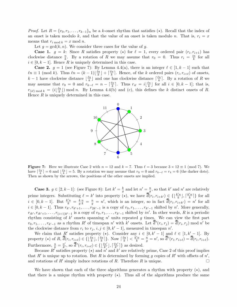
Case 3. g ∈ [2, k−1]: (see Figure 8): Let k′ = kg and let n′ = n
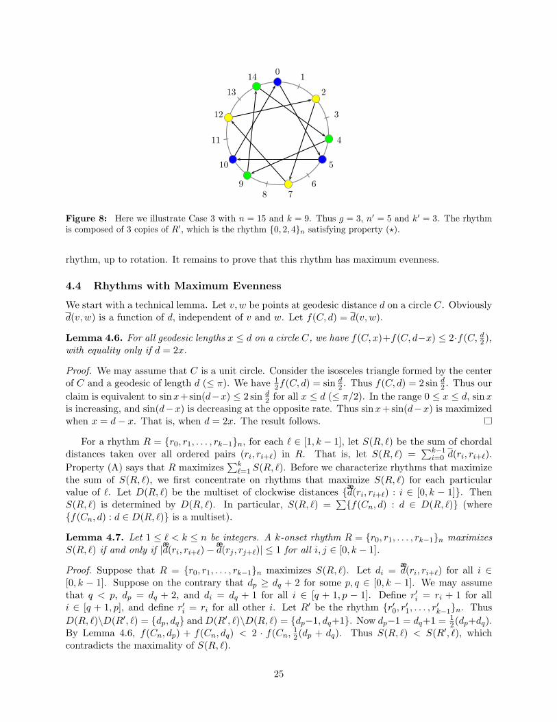
g , so that k′ and n′ are relatively
prime integers. Substituting ` = k′ into property (?), we haveñd(ri, ri+k′) ∈ bk
′nk c, d
k′nk e for all
i ∈ [0, k − 1]. But k′nk = k
gnk = n
g = n′, which is an integer, so in factñd(ri, ri+k′) = n′ for all
i ∈ [0, k − 1]. Thus rk′ , rk′+1, . . . , r2k′−1 is a copy of r0, r1, . . . , rk′−1 shifted by n′. More generally,rik′ , rik′+1, . . . , r(i+1)k′−1 is a copy of r0, r1, . . . , rk′−1 shifted by in′. In other words, R is a periodicrhythm consisting of k′ onsets spanning n′ units repeated g times. We can view the first partr0, r1, . . . , rk′−1 as a rhythm R′ of timespan n′ with k′ onsets. Let
ñd ′(ri, rj) =
ñd(ri, rj) mod n′ be
the clockwise distance from ri to rj , i, j ∈ [0, k′ − 1], measured in timespan n′.We claim that R′ satisfies property (?). Consider any i ∈ [0, k′ − 1] and ` ∈ [1, k′ − 1]. By
property (?) of R,ñd(ri, ri+`) ∈ b `n
k c, d`nk e. Now d `nk e < k′n
k = ng = n′, so
ñd ′(ri, ri+`) =
ñd(ri, ri+`).
Furthermore, nk = n′
k′ , soñd ′(ri, ri+`) ∈ b `n′
k′ c, d`n′
k′ e as desired.Because R′ satisfies property (?) and n′ and k′ are relatively prime, Case 2 of this proof implies
that R′ is unique up to rotation. But R is determined by forming g copies of R′ with offsets of n′,and rotations of R′ simply induce rotations of R. Therefore R is unique.
We have shown that each of the three algorithms generates a rhythm with property (?), andthat there is a unique rhythm with property (?). Thus all of the algorithms produce the same
24
01
2
3
4
5
6
78
9
10
11
12
13
14
Figure 8: Here we illustrate Case 3 with n = 15 and k = 9. Thus g = 3, n′ = 5 and k′ = 3. The rhythmis composed of 3 copies of R′, which is the rhythm 0, 2, 4n satisfying property (?).
rhythm, up to rotation. It remains to prove that this rhythm has maximum evenness.
4.4 Rhythms with Maximum Evenness
We start with a technical lemma. Let v, w be points at geodesic distance d on a circle C. Obviouslyd(v, w) is a function of d, independent of v and w. Let f(C, d) = d(v, w).
Lemma 4.6. For all geodesic lengths x ≤ d on a circle C, we have f(C, x)+f(C, d−x) ≤ 2·f(C, d2),
with equality only if d = 2x.
Proof. We may assume that C is a unit circle. Consider the isosceles triangle formed by the centerof C and a geodesic of length d (≤ π). We have 1
2f(C, d) = sin d2 . Thus f(C, d) = 2 sin d
2 . Thus ourclaim is equivalent to sinx+sin(d−x) ≤ 2 sin d
2 for all x ≤ d (≤ π/2). In the range 0 ≤ x ≤ d, sinxis increasing, and sin(d−x) is decreasing at the opposite rate. Thus sinx+sin(d−x) is maximizedwhen x = d− x. That is, when d = 2x. The result follows.
For a rhythm R = r0, r1, . . . , rk−1n, for each ` ∈ [1, k − 1], let S(R, `) be the sum of chordaldistances taken over all ordered pairs (ri, ri+`) in R. That is, let S(R, `) =
∑k−1i=0 d(ri, ri+`).
Property (A) says that R maximizes∑k
`=1 S(R, `). Before we characterize rhythms that maximizethe sum of S(R, `), we first concentrate on rhythms that maximize S(R, `) for each particularvalue of `. Let D(R, `) be the multiset of clockwise distances ñd(ri, ri+`) : i ∈ [0, k − 1]. ThenS(R, `) is determined by D(R, `). In particular, S(R, `) =
∑f(Cn, d) : d ∈ D(R, `) (where
f(Cn, d) : d ∈ D(R, `) is a multiset).
Lemma 4.7. Let 1 ≤ ` < k ≤ n be integers. A k-onset rhythm R = r0, r1, . . . , rk−1n maximizesS(R, `) if and only if |ñd(ri, ri+`)−
ñd(rj , rj+`)| ≤ 1 for all i, j ∈ [0, k − 1].
Proof. Suppose that R = r0, r1, . . . , rk−1n maximizes S(R, `). Let di =ñd(ri, ri+`) for all i ∈
[0, k − 1]. Suppose on the contrary that dp ≥ dq + 2 for some p, q ∈ [0, k − 1]. We may assumethat q < p, dp = dq + 2, and di = dq + 1 for all i ∈ [q + 1, p − 1]. Define r′i = ri + 1 for alli ∈ [q + 1, p], and define r′i = ri for all other i. Let R′ be the rhythm r′0, r′1, . . . , r′k−1n. ThusD(R, `)\D(R′, `) = dp, dq and D(R′, `)\D(R, `) = dp−1, dq+1. Now dp−1 = dq+1 = 1
2(dp+dq).By Lemma 4.6, f(Cn, dp) + f(Cn, dq) < 2 · f(Cn, 1
2(dp + dq). Thus S(R, `) < S(R′, `), whichcontradicts the maximality of S(R, `).
25
For the converse, let R be a rhythm such that |ñd(ri, ri+`)−ñd(rj , rj+`)| ≤ 1 for all i, j ∈ [0, k−1].
Suppose on the contrary that R does not maximize S(R, `). Thus some rhythm T = (t0, t1, . . . , tk−1)maximizes S(T, `) and T 6= R. Hence D(T, `) 6= D(R, `). Since
∑D(R, `) =
∑D(T, `) (= `n), we
haveñd(ti, ti+`) −
ñd(tj , tj+`) ≥ 2 for some i, j ∈ [0, k − 1]. As we have already proved, this implies
that T does not maximize S(T, `). This contradiction proves that R maximizes S(R, `).
Since∑k−1
i=0
ñd(ri, ri+`) = `n for any rhythm with k onsets and timespan n, Lemma 4.7 can be
restated as follows.
Corollary 4.8. Let 1 ≤ ` < k ≤ n be integers. A k-onset rhythm R = r0, r1, . . . , rk−1n maximizesS(R, `) if and only if
ñd(ri, ri+`) ∈ d `n
k e, b`nk c for all i ∈ [0, k − 1].
Proof (?) ⇒ (A). If (?) holds for some rhythm R, then by Corollary 4.8, R maximizes S(R, `) forevery `. Thus R maximizes
∑` S(R, `).
Proof (A) ⇒ (?). By Theorem 4.5, there is a unique rhythm R that satisfies property (?). Let Rdenote the unique rhythm that satisfies property (?). Suppose on the contrary that there is a rhythmT = (t0, t1, . . . , tk−1) with property (A) but R 6= T . Thus there exists an ordered pair (ti, ti+`) inT with clockwise distance
ñd(ti, ti+`) 6∈ b `nk c, d
`nk e. By Corollary 4.8, S(T, `) < S(R, `). Since T
has property (A),∑k
`=1 S(T, `) ≥∑k
`=1 S(R, `). Thus for some `′ we have S(T, `′) > S(R, `′). Butthis is a contradiction, because S(R, `′) ≥ S(T, `′) by Corollary 4.8.
This completes the proof of Theorem 4.1. We now show that Theorem 4.1 can be generalized forother metrics that satisfy Lemma 4.6. To formalize this idea we introduce the following definition.A function g : [0, π] → R+ ∪ 0 is halving if for all geodesic lengths x ≤ d ≤ π on the unit circle,g(x) + g(d− x) ≤ 2 · g(d
2), with equality only if d = 2x. For example, chord length is halving, butgeodesic distance is not (because we have equality for all x). Observe that the proof of Lemma 4.7and Corollary 4.8 depend on this property alone. Thus we have the following generalization ofTheorem 4.1.
Theorem 4.9. Let n ≥ k ≥ 2 be integers. Let g be a halving function. The following are equivalentfor a rhythm R = (r0, r1, . . . , rk−1) with n pulses and k onsets:
(A) R maximises∑k−1
i=0
∑k−1j=i+1 g(
òd(ri, rj)),
(B) R is determined by the Clough-Douthett(k, n) algorithm,
(C) R is determined by the Snap(k, n) algorithm,
(D) R is determined by the Euclidean(k, n) algorithm,
(?) for all ` ∈ [1, k − 1] and i ∈ [0, k − 1], the ordered pair (ri, ri+`) has clockwise distanced(ri, ri+`) ∈ b `n
k c, d`nk e.
Moreover, up to a rotation, there is a unique rhythm that satisfies these conditions.
26
5 Deep Rhythms
Recall that a rhythm is Winograd-deep if every geodesic distance 1, 2, . . . , bn2 c has a unique multi-plicity; it is Erdos-deep if the multiplicity of every geodesic distance defined by pairs of onsets inunique. Winograd [Win66], and independently Clough et al. [CEK99], characterize all Winograd-deep scales: up to rotation, they are the scales that can be generated by the first bn2 c or bn2 c + 1multiples (modulo n) of a value that is relatively prime to n, plus one exceptional scale 0, 1, 2, 46.In this section, we prove a similar (but more general) characterization of Erdos-deep rhythms: up torotation and scaling, they are the rhythms generable as the first k multiples (modulo n) of a valuethat is relatively prime to n, plus the same exceptional rhythm 0, 1, 2, 46. The key difference isthat the number of onsets k is now a free parameter, instead of being forced to be either bn2 c orbn2 c+ 1. Our proof follows Winograd’s, but differs in one case (the second case of Theorem 5.3).
We later prove that every Erdos-deep rhythm has a shelling and that maximally even rhythmswith n and k relatively prime are Erdos-deep.
5.1 Characterization of Deep Rhythms
Our characterization of Erdos-deep rhythms is in terms of two families of rhythms. The mainrhythm family consists of the generated rhythms Dk,n,m = im mod n : i = 0, 1, . . . , k − 1n oftimespan n, for certain values of k, n, and m. The one exceptional rhythm is F = 0, 1, 2, 46 oftimespan 6.
Fact 5.1. F is Erdos-deep.
Lemma 5.2. If k ≤ bn2 c+ 1 and m and n are relatively prime, then Dk,n,m is Erdos-deep.
Proof. The multiset of clockwise distances in Dk,n,m is (jm− im) mod n : i < j = (j− i)m modn : i < j. There are k−p choices of i and j such that j−i = p, so there are exactly p occurrences ofthe clockwise distance (pm) mod n in the multiset. Each of these clockwise distances correspondsto a geodesic distance—either (pm) mod n or (−pm) mod n, whichever is smaller (at most n
2 ). Weclaim that these geodesic distances are all distinct. Then the multiplicity of each geodesic distance(±pm) mod n is exactly p, establishing that the rhythm is Erdos-deep.
For two geodesic distances to be equal, we must have ±pm ≡ ±qm (mod n) for some (possiblydifferent) choices for the ± symbols, and for some p 6= q. By (possibly) multiplying both sides by−1, we obtain two cases: (1) pm ≡ qm (mod n) and (2) pm ≡ −qm (mod n). Since m is relativelyprime to n, by Lemma 4.2, m has a multiplicative inverse modulo n. Multiplying both sides ofthe congruence by this inverse, we obtain (1) p ≡ q (mod n) and (2) p ≡ −q (mod n). Since0 ≤ i < j < k ≤ bn2 c + 1, we have 0 ≤ p = j − i < bn2 c + 1, and similarly for q: 0 ≤ p, q ≤ bn2 c.Thus, the first case of p ≡ q (mod n) can happen only when p = q, and the second case of p+ q ≡ 0(mod n) can happen only when p = q = 0 or when p = q = n
2 . Either case contradicts that p 6= q.Therefore the geodesic distances arising from different values of p are indeed distinct, proving thelemma.
We now state and prove our characterization of Erdos-deep rhythms, which is up to rotationand scaling. Rotation preserves the geodesic distance multiset and therefore Erdos-deepness (andWinograd-deepness). Scaling maps each geodesic distance d to αd, and thus preserves multiplicitiesand therefore Erdos-deepness (but not Winograd-deepness). Note that the rhythm Dk,n,m is arotation by −m(k − 1) mod n of the rhythm Dk,n,n−m; to avoid this duplication we restrict m tobe equal to at most bn2 c.
27
Theorem 5.3. A rhythm is Erdos-deep if and only if it is a rotation of a scaling of either therhythm F or the rhythm Dk,n,m for some k, n,m with k ≤ bn2 c+ 1, 1 ≤ m ≤ bn2 c, and m and n arerelatively prime.
Proof. Since a rotation of a scaling of an Erdos-deep rhythm is Erdos-deep, the “if” direction ofthe theorem follows from Fact 5.1 and Lemma 5.2.
Consider an Erdos-deep rhythm R with k onsets. By the definition of Erdos-deepness, R hasone nonzero geodesic distance with multiplicity i for each i = 1, 2, . . . , k− 1. Let m be the geodesicdistance with multiplicity k − 1. Since m is a geodesic distance, 1 ≤ m ≤ bn2 c. Also, k ≤ bn2 c + 1(for any Erdos-deep rhythm R), because all nonzero geodesic distances are between 1 and bn2 c andtherefore at most bn2 c nonzero geodesic distances occur. Thus k and m are suitable parameterchoices for Dk,n,m.
Consider the graph Gm = (R,Em) with vertices corresponding to onsets in R and with an edgebetween two onsets of geodesic distance m. By the definition of geodesic distance, every vertex i inGm has degree at most 2: the only onsets at geodesic distance exactly m from i are (i−m) mod nand (i + m) mod n. Thus, the graph Gm is a disjoint union of paths and cycles. The number ofedges in Gm is the multiplicity of m, which we supposed was k−1, which is 1 less than the numberof vertices in Gm. Thus, the graph Gm consists of exactly one path and any number of cycles.
The cycles of Gm have a special structure because they correspond to subgroups generated bysingle elements in the cyclic group (Z/(n),+). Namely, the onsets corresponding to vertices of acycle in Gm form a regular (n
a )-gon, with a geodesic distance of a = gcd(m,n) between consecutiveonsets. (a is called the index of the subgroup generated by m.) In particular, every cycle in Gm
has the same length r = na . Since Gm is a simple graph, every cycle must have at least 3 vertices,
so r ≥ 3.The proof consists of four cases depending on the length of the path and on how many cycles
the graph Gm has. The first two cases will turn out to be impossible; the third case will lead to arotation of a scaling of rhythm F ; and the fourth case will lead to a rotation of a scaling of Dk,n,m.
First suppose that the graph Gm consists of a path of length at least 1 and at least one cycle.We show that this case is impossible because the rhythm R can have no geodesic distance withmultiplicity 1. Suppose that there is a geodesic distance with multiplicity 1, say between onsets i1and i2. If i is a vertex of a cycle, then both (i + m) mod n and (i−m) mod n are onsets in R. Ifi is a vertex of the path, then one or two of these are onsets in R, with the case of one occurringonly at the endpoints of the path. If (i1 + m) mod n and (i2 + m) mod n were both onsets in R, or(i1−m) mod n and (i2−m) mod n were both onsets in R, then we would have another occurrence ofthe geodesic distance between i1 and i2, contradicting that this geodesic distance has multiplicity 1.Thus, i1 and i2 must be opposite endpoints of the path. If the path has length `, then the clockwisedistance between i1 and i2 is (`m) mod n. This clockwise distance (and hence the correspondinggeodesic distance) appears in every cycle, of which there is at least one, so the geodesic distancehas multiplicity more than 1, a contradiction. Therefore this case is impossible.
Second suppose that the graph Gm consists of a path of length 0 and at least two cycles. Weshow that this case is impossible because the rhythm R has two geodesic distances with the samemultiplicity. Pick any two cycles C and C ′, and let d be the smallest positive clockwise distancefrom a vertex of C to a vertex of C ′. Thus i is a vertex of C if and only if (i + d) mod n is avertex of C ′. Since the cycles are disjoint, d < a. Since r ≥ 3, d < n
3 , so clockwise distances ofd are also geodesic distances of d. The number of occurrences of geodesic distance d between avertex of C and a vertex of C ′ is either r or 2r, the case of 2r arising when d = a
2 (that is, C ′ is a“half-rotation” of C). The number of occurrences of geodesic distance d′ = mind+m,n−(d+m)is the same—either r or 2r, in the same cases. (Note that d < a ≤ n − m, so d + m < n, so
28
the definition of d′ correctly captures a geodesic distance modulo n.) The same is true of geodesicdistance d′′ = mind −m,n − (d −m). If other pairs of cycles have the same smallest positiveclockwise distance d, then the number of occurrences of d, d′, and d′′ between those cycles arealso equal. Since the cycles are disjoint, geodesic distance d and thus d + m and d−m cannot be(pm) mod n for any p, so these geodesic distances cannot occur between two vertices of the samecycle. Finally, the sole vertex x of the path has geodesic distance d to onset i (which must be avertex of some cycle) if and only if x has geodesic distance d′ to onset (i + m) mod n (which mustbe a vertex of the same cycle) if and only if x has geodesic distance d′′ to onset (i − m) mod n(which also must be a vertex of the same cycle). Therefore the multiplicities of geodesic distancesd, d′, and d′′ must be equal. Since R is Erdos-deep, we must have d = d′ = d′′. To have d = d′,either d = d+m or d = n− (d+m), but the first case is impossible because d > 0 by nonoverlap ofcycles, so 2d + m = n. Similarly, to have d = d′′, we must have 2d−m = n. Subtracting these twoequations, we obtain that 2m = 0, contradicting that m > 0. Therefore this case is also impossible.
Third suppose that the graph Gm consists of a path of length 0 and exactly one cycle. We showthat this case forces R to be a rotation of a scaling of rhythm F because otherwise two geodesicdistances m and m′ have the same multiplicity. The number of occurrences of geodesic distance min the cycle is precisely the length r of the cycle. Similarly, the number of occurrences of geodesicdistance m′ = min2m,n − 2m in the cycle is r. The sole vertex x on the path cannot havegeodesic distance m or m′ to any other onset (a vertex of the cycle) because x would then be onthe cycle. Therefore the multiplicities of geodesic distances m and m′ must be equal. Since R isErdos-deep, m must equal m′, which implies that either m = 2m or m = n− 2m. The first case isimpossible because m > 0. In the second case, 3m = n, that is, m = n
3 . Therefore, the cycle hasr = 3 vertices, say at ∆,∆+ n
3 ,∆+ 2n3 . The fourth and final onset x must be midway between two
of these three onsets, because otherwise its geodesic distance to the three vertices are all distinctand therefore unique. No matter where x is so placed, the rhythm R is a rotation by ∆ + cn
3 (forsome c ∈ 0, 1, 2) of a scaling by n
6 of the rhythm F .Finally suppose that Gm has no cycles, and consists solely of a path. We show that this case
forces R to be a rotation of a scaling of a rhythm Dk,n′,m′ with 1 ≤ m′ ≤ bn′2 c and with m′ and n′
relatively prime. Let i be the onset such that (i−m) mod n is not an onset (the “beginning” vertex ofthe path). Consider rotating R by −i so that 0 is an onset in the resulting rhythm R−i. The verticesof the path in R− i form a subset of the subgroup of the cyclic group (Z/(n),+) generated by theelement m. Therefore the rhythm R− i = Dk,n,m = (im) mod n : i = 0, 1, . . . , k− 1n is a scalingby a of the rhythm Dk,n/a,m/a = ( im
a ) mod (na ) : i = 0, 1, . . . , k − 1n. The rhythm Dk,n/a,m/a
has an appropriate value for the third argument: ma and n
a are relatively prime (a = gcd(m,n))
and 1 ≤ ma ≤
bn/2ca ≤
⌊n/a2
⌋. Also, k ≤
⌊n/a2
⌋+ 1 because the only occurring geodesic distances
are multiples of a and therefore the number k − 1 of distinct geodesic distances is at most⌊
n/a2
⌋.
Therefore R is a rotation by i of a scaling by a of Dk,n/a,m/a with appropriate values of thearguments.
Corollary 5.4. A rhythm is Erdos-deep if and only if it is a rotation of a scaling of the rhythm For it is a rotation of a rhythm Dk,n,m for some k, n,m satisfying k ≤ b n
2g c+1 where g = gcd(m,n).
Proof. First we show that any Erdos-deep rhythm has one of the two forms in the corollary. ByTheorem 5.3, there are two flavors of Erdos-deep rhythms, and the corollary directly handlesrotations of scalings of F . Thus it suffices to consider a rhythm R that is a rotation by ∆ of a scalingby α of Dk,n,m where k ≤ bn2 c+ 1, 1 ≤ m ≤ bn2 c, and m and n are relatively prime. Equivalently,R is a rotation by ∆ of Dk,n′,m′ where n′ = αn and m′ = αm. Now g = gcd(n′,m′) = α, so n′
g = n.
29
Hence, k ≤ b n′
2g c+ 1 as desired. Thus we have rewritten R in the desired form.It remains to show that every rhythm in one of the two forms in the corollary is Erdos-deep.
Again, rotations of scalings of F are handled directly by Theorem 5.3. So consider a rotation ofDk,n,m where k ≤ b n
2g c+1. The value of m matters only modulo n, so we assume that 0 ≤ m ≤ n−1.First we show that, if bn2 c+ 1 ≤ m ≤ n− 1, then Dk,n,m can be rewritten as a rotation of the
rhythm Dk,n,m′ where m′ = n −m ≤ bn2 c. By reversing the order in which we list the onsets inDk,n,m = im mod n : i = 0, 1, . . . , k − 1n, we can write Dk,n,m = (k − 1 − i) m mod n : i =0, 1, . . . , k−1n. Now consider rotating the rhythm Dk,n,n−m = i (n−m) mod n : i = 0, 1, . . . , k−1n by (k − 1)m. We obtain the rhythm [i (n −m) + (k − 1) m] mod n : i = 0, 1, . . . , k − 1n =[(k−1−i) m+in] mod n : i = 0, 1, . . . , k−1n = (k−1−i) m mod n : i = 0, 1, . . . , k−1n = Dk,n,m
as desired.Thus it suffices to consider rotations of Dk,n,m where 1 ≤ m ≤ bn
2 c and k ≤ b n2g c. The rhythm
Dk,n′,m′ , where n′ = ng and m′ = m
g , is Erdos-deep by Theorem 5.3 because n′ and m′ are relatively
prime, k ≤ bn′2 c+ 1, and 1 ≤ m′ ≤ bn′2 c. But Dk,n,m is the scaling of Dk,n′,m′ by the integer g, soDk,n,m is also Erdos-deep.
An interesting consequence of this characterization is the following:
Corollary 5.5. Every Erdos-deep rhythm has a shelling.
Proof. If the Erdos-deep rhythm is Dk,n,m, we can remove the last onset from the path, resultingin Dk−1,n,m, and repeat until we obtain the empty rhythm D0,n,m. At all times, k remains at mostbn2 c+ 1 (assuming it was originally) and m remains between 1 and bn2 c and relatively prime to n.On the other hand, F = 0, 1, 2, 46 has the shelling 4, 2, 1, 0 because 0, 1, 26 is Erdos-deep.
We can generalize this characterization of Erdos-deep rhythms to the continuous case where n isan arbitrary real number, and onsets can be at arbitrary (not necessarily integer) points along thecircle. We will call such rhythms continuous rhythms. In this case we have two kinds of rhythms.First, if m and n are rational multiples of each other, we can scale the rhythm by some rational psuch that pm and pn are integers, and apply Theorem 5.3 using pn and pm to characterize all deeprhythms where m is a rational multiple of n. Second, if m and n are irrational multiples of eachother, we can show that every Dk,n,m is Erdos-deep. The complete characterization of continuousErdos-deep rhythms is as follows:
Theorem 5.6. A continuous rhythm is Erdos-deep if and only if it is a rotation of a scaling ofDk,n,m with k ≤ bn2 c+1, 0 < m ≤ n
2 , and where m and n are either (1) irrational multiples of eachother, or (2) rational multiples such that for some rational p, integers pm and pn are relativelyprime.
Proof. To prove the “if” direction, we show that all geodesic distances defined by Dk,n,m are distinct;hence we need to prove that the multiplicity of each geodesic distance (±pm) mod n is exactly p.First assume that m and n are irrational multiples of each other, i.e., there is no rational numberthat divides both m and n. Suppose two geodesic distances±pm ≡ ±qm (mod n) for some (possiblydifferent) choices for the ± symbols, and for some p 6= q. Then we can write ±pm = ±qm + rnfor some integer r. This in turn implies that m = r
±p∓qn, which contradicts the fact that m andn are irrational multiples of each other. Therefore, when m and n are irrational multiples of eachother, the geodesic distances arising from different values of p are distinct, proving that Dk,n,m isErdos-deep.
30

If m and n are rational multiples of each other, then so are each of the geodesic distances2m, 3m, . . . (k − 1)m (mod n) with n. In this case, there exists a rational p such that pn and pmare both integers. We can now apply Theorem 5.3 using pn and pm, and generate all deep rhythmswhere m is a rational multiple of n.
For the “only if” direction, consider a continuous Erdos-deep rhythm R with k onsets and periodn, and with some geodesic distance m having multiplicity k−1. Consider the graph Gm = (R,Em)as defined in the proof of Theorem 5.3 (with vertices corresponding to onsets in R and with anedge between two onsets of geodesic distance m). If m and n are rational multiples of each other,then we can scale R by some rational p and apply Theorem 5.3 to show that R is a scaling by 1
p ofDk,pn,pm where pm and pn are relatively prime integers and 1 ≤ pm ≤ bpn
2 c, so 0 < m ≤ n2 .
If m and n are irrational multiples of each other, then there is no rational number r such thatn = rm. This means that Gm cannot contain a cycle, so consists of a single path of length k − 1.As in the proof of Theorem 5.3, we can rotate R by −i so that 0 is an onset in the resultingrhythm R− i. The vertices of the path in R− i form a subset of the subgroup of the cyclic group(Z/(n),+) generated by the element m. Therefore the rhythm R− i = Dk,n,m = (im) mod n : i =0, 1, . . . , k − 1n where m and n are irrational multiples of each other and 0 < m ≤ n
2 .
5.2 Connection Between Deep and Even Rhythms
A connection between maximally even scales and Winograd-deep scales is shown by Clough etal. [CEK99]. They define a diatonic scale to be a maximally even scale with k = n+2
2 and n amultiple of 4. They show that diatonic scales are Winograd-deep. We now prove a similar resultfor Erdos-deep rhythms.
Lemma 5.7. A rhythm R of maximum evenness satisfying k ≤ bn2 c+ 1 is Erdos-deep if and only
if k and n are relatively prime.
Proof. Recall that by property (?) one of the unique characterizations of an even rhythm of max-imum evenness can be stated as follows. For all ` ∈ [1, k − 1], and for every ordered pair (ri, ri+`)of onsets in R, the clockwise distance
ñd(ri, ri+`) ∈ b `n
k c, d`nk e.
For the case in which k and n are relatively prime, by Lemma 4.2, there exists a value ` < ksuch that `n ≡ 1 (mod k). Thus we can write `n = kb`n
k c+1. Let m = b`nk c. Now consider the set
im mod n : i = 0, 1, . . . , k − 1n. By Lemma 4.4(c), we get k distinct values, so R can be realizedas Dk,n,m = im mod n : i = 0, 1, . . . , k − 1n. Thus, by Lemma 5.2, R is Erdos-deep.
Observe that F = 0, 1, 2, 46 does not maximize evenness becauseñd(0, 2) = 2 and
ñd(2, 0) = 4
yet ` = 2. Hence, any rhythm that maximizes evenness and that is deep must also be generated.Now consider the case in which n and k are not relatively prime. We show that the assumption
that R is deep leads to a contradiction. Thus, assuming that R is deep implies that there is a valuem such that R can be realized as Dk,n,m = im mod n : i = 0, 1, . . . , k − 1n. This in turn impliesthat there exists an integer ` such that km = `n + 1, that is, `n ≡ 1 (mod k). However, for this tohappen, n and k must be relatively prime, a contradiction.
Thus we have shown that R is Erdos-deep if and only if k and n are relatively prime.
Acknowledgments
This work was initiated at the 20th Bellairs Winter Workshop on Computational Geometry heldJanuary 28–February 4, 2005 at Bellairs Research Institute in Barbados. We thank the otherparticipants of that workshop—Greg Aloupis, David Bremner, Justin Colannino, Mirela Damian,
31
Vida Dujmovic, Jeff Erickson, Ferran Hurtado, John Iacono, Danny Krizanc, Stefan Langerman,Erin McLeish, Pat Morin, Mark Overmars, Suneeta Ramaswami, Diane Souvaine, Ileana Streinu,Remco Veltcamp, and Sue Whitesides—for helpful discussions and contributing to a fun and creativeatmosphere.
Thanks to Simha Arom for providing us with a copy of his paper on the classification of aksakrhythms [Aro04], which provided several examples of Euclidean rhythms of which we were not aware.Thanks to Jeff Erickson for bringing to our attention the wonderful paper by Mitchell Harris andEd Reingold [HR04] on digital line drawing, leap year calculations, and Euclid’s algorithm. Thanksto Marcia Ascher for pointing out that the leap-year pattern of the Jewish calendar is a Euclideanrhythmic necklace.
The proof of Case 3 in Theorem 4.5, which is substantially simpler than our original proof, isbased on a suggestion from Dmitri Tymoczko.
Finally, we would like to thank the two referees for useful comments.
References
[Aga86] V. Kofi Agawu. Gi Dunu, Nyekpadudo, and the study of West African rhythm.Ethnomusicology, 30(1):64–83, Winter 1986.
[Ank97] Willie Anku. Principles of rhythm integration in African music. Black Music ResearchJournal, 17(2):211–238, Autumn 1997.
[Aro91] Simha Arom. African Polyphony and Polyrhythm. Cambridge University Press, Cam-bridge, England, 1991.
[Aro04] Simha Arom. L’aksak: Principes et typologie. Cahiers de Musiques Traditionnelles,17:12–48, 2004.
[AS02] Jean-Paul Allouche and Jeffrey O. Shallit. Automatic Sequences. Cambridge UniversityPress, Cambridge, England, 2002.
[Asc75] Michael I. Asch. Social context and the musical analysis of Slavey drum dance songs.Ethnomusicology, 19(2):245–257, May 1975.
[Asc02] Marcia Ascher. Mathematics Elsewhere: An Exploration of Ideas Across Cultures.Princeton University Press, Princeton and Oxford, 2002.
[Ash03] Anthony Ashton. Harmonograph–A Visual Guide to the Mathematics of Music. Walkerand Company, New York, 2003.
[Bar81] Bela Bartok. Ce qu’on appelle le rythme bulgare. In Musique de la vie, pages 142–155,Stock, Paris, 1981.
[Bar04a] James M. Barbour. Tuning and Temperament: A Historical Survey. Dover, New York,2004.
[Bar04b] Gregory Barz. Music in East Africa. Oxford University Press, Oxford, England, 2004.
[BD94] Steven Block and Jack Douthett. Vector products and intervallic weighting. Journalof Music Theory, 38:21–41, 1994.
[Beh73] Gerard Behague. Bossa and bossas: recent changes in Brazilian urban popular music.Ethnomusicology, 17(2):209–233, 1973.
[Bek05] Tolga Bektas. Relationships between prosodic and musical meters in the Beste formof classical Turkish music. Asian Music, 36(1):1–26, Winter/Spring 2005.
32
[Bjo03a] Eric Bjorklund. A metric for measuring the evenness of timing system rep-rate pat-terns. SNS ASD Technical Note SNS-NOTE-CNTRL-100, Los Alamos National Lab-oratory, Los Alamos, U.S.A., 2003.
[Bjo03b] Eric Bjorklund. The theory of rep-rate pattern generation in the SNS timing system.SNS ASD Technical Note SNS-NOTE-CNTRL-99, Los Alamos National Laboratory,Los Alamos, U.S.A., 2003.
[Bra51] Constantin Brailoiu. Le rythme aksak. Revue de Musicologie, 33:71–108, 1951.
[Bre65] Jack E. Bresenham. Algorithm for computer control of digital plotter. IBM SystemsJournal, 4:25–30, 1965.
[Bre99] Roy Brewer. The use of Habanera rhythm in rockabilly music. American Music,17:300–317, Autumn 1999.
[Bru64] Viggo Brun. Euclidean algorithms and musical theory. Enseignement Mathematique,10:125–137, 1964.
[Car98] Norman Carey. Distribution modulo 1 and musical scales. PhD thesis, University ofRochester, Rochester, New York, 1998.
[CD91] John Clough and Jack Douthett. Maximally even sets. Journal of Music Theory,35:93–173, 1991.
[CEK99] John Clough, Nora Engebretsen, and Jonathan Kochavi. Scales, sets, and intervalcycles: a taxonomy. Music Theory Spectrum, 21(1):74–104, Spring 1999.
[Che79] John Miller Chernoff. African Rhythm and African Sensibility. The University ofChicago Press, Chicago, 1979.
[Che91] John Miller Chernoff. The rhythmic medium in african music. New Literary History,22(4):1093–1102, Autumn 1991. Papers from the Commonwealth Center for Literaryand Cultural Change.
[Che02] Marc Chemillier. Ethnomusicology, ethnomathematics. The logic underlying orallytransmitted artistic practices. In Gerard Assayag, Hans Georg Feichtinger, andJose Francisco Rodrigues, editors, Mathematics and Music, pages 161–183. Springer-Verlag, 2002.
[Cla00] Martin Clayton. Time in Indian Music. Oxford University Press, New York, 2000.
[Cle94] Jerome Cler. Pour une theorie de l’aksak. Revue de Musicologie, 80:181–210, 1994.
[CLRS01] Thomas H. Cormen, Charles E. Leiserson, Ronald L. Rivest, and Clifford Stein. In-troduction to Algorithms. The MIT Press, Cambridge, Massachussetts, 2001.
[CM85] John Clough and Gerald Myerson. Variety and multiplicity in diatonic systems. Jour-nal of Music Theory, 29:249–270, 1985.
[CM86] John Clough and Gerald Myerson. Musical scales and the generalized circle of fifths.American Mathematical Monthly, 93(9):695–701, 1986.
[Cox62] H. S. M. Coxeter. Music and mathematics. The Canadian Music Journal, VI:13–24,1962.
[CT03] Marc Chemillier and Charlotte Truchet. Computation of words satisfying the “rhyth-mic oddity property” (after Simha Arom’s works). Information Processing Letters,86:255–261, 2003.
[CW95] Patricia Shehan Campbell and Christopher Waterman. Christopher Waterman onYoruba music of Africa. Music Educator’s Journal, 81(6):35–43, 1995.
33
[DBFG+04] Miguel Dıaz-Banez, Giovanna Farigu, Francisco Gomez, David Rappaport, and God-fried T. Toussaint. El compas flamenco: a phylogenetic analysis. In Proceedings ofBRIDGES: Mathematical Connections in Art, Music and Science, Southwestern Col-lege, Winfield, Kansas, July 30 - August 1 2004.
[EMF90] Issam El-Mallah and Kai Fikentscher. Some observations on the naming of musicalinstruments and on the rhythm in Oman. Yearbook for Traditional Music, 22:123–126,1990.
[Erd89] Paul Erdos. Distances with specified multiplicities. American Mathematical Monthly,96:447, 1989.
[ERSS03] John Ellis, Frank Ruskey, Joe Sawada, and Jamie Simpson. Euclidean strings. Theo-retical Computer Science, 301:321–340, 2003.
[Euc56] Euclid. Elements. Dover, 1956. Translated by Sir Thomas L. Heath.
[Eva66] Bob Evans. Authentic Conga Rhythms. Belwin Mills Publishing Corporation, Miami,1966.
[Far92] Mary Farquharson. Africa in America. Discos Corazon, Mexico, 1992. [CD].
[Flo99] Samuel A. Floyd, Jr. Black music in the circum-Caribbean. American Music, 17(1):1–38, 1999.
[For73] Allen Forte. The Structure of Atonal Music. Yale Univ. Press, New Haven, Connecti-cut, U.S.A., 1973.
[Fra56] Philip Franklin. The Euclidean algorithm. The American Mathematical Monthly,63(9):663–664, November 1956.
[Gam67a] Carlton Gamer. Deep scales and difference sets in equal-tempered systems. In Proceed-ings of the 2nd Annual Conference of the American Society of University Composers,pages 113–122, 1967.
[Gam67b] Carlton Gamer. Some combinational resources of equal-tempered systems. Journal ofMusic Theory, 11:32–59, 1967.
[GMRT05] Francisco Gomez, Andrew Melvin, David Rappaport, and Godfried T. Toussaint.Mathematical measures of syncopation. In Proc. BRIDGES: Mathematical Connec-tions in Art, Music and Science, pages 73–84, Banff, Alberta, Canada, July 31 -August 3 2005.
[Hag03] Kobi Hagoel. The Art of Middle Eastern Rhythm. OR-TAV Music Publications, KfarSava, Israel, 2003.
[Has97] Christopher F. Hasty. Meter as Rhythm. Oxford University Press, Oxford, England,1997.
[HK81] Lee Hye-Ku. Quintuple meter in Korean instrumental music. Asian Music, 13(1):119–129, 1981.
[HR04] Mitchell A. Harris and Edward M. Reingold. Line drawing, leap years, and Euclid.ACM Computing Surveys, 36(1):68–80, March 2004.
[HT07] Rachel Hall and Dmitri Tymoczko. Voice leading, submajorization, and the distribu-tion constraint. Preprint, 2007.
[Joh03] Timothy A. Johnson. Foundations of Diatonic Theory: A Mathematically Based Ap-proach to Music Fundamentals. Key College Publishing, Emeryville, California, 2003.
34
[Kau80] Robert Kauffman. African rhythm: A reassessment. Ethnomusicology, 24(3):393–415,September 1980.
[Kei91] Michael Keith. From Polychords to Polya: Adventures in Musical Combinatorics.Vinculum Press, Princeton, 1991.
[Klo97] Tom Klower. The Joy of Drumming: Drums and Percussion Instruments from Aroundthe World. Binkey Kok Publications, Diever, Holland, 1997.
[Knu98] Donald E. Knuth. The Art of Computer Programming, volume 2, 3rd edition. AddisonWesley, Reading, Massachussets, 1998.
[Koe70] James Koetting. Analysis and notation of West African drum ensemble music. Pub-lications of the Institute of Ethnomusicology, 1(3), 1970.
[KR04] Reinhard Klette and Azriel Rosenfeld. Digital straightness - a review. Discrete AppliedMathematics, 139:197–230, 2004.
[Log84] Wendell Logan. The ostinato idea in black improvised music: A preliminary investi-gation. The Black Perspecyive in Music, 12(2):193–215, 1984.
[Lon04] Justin London. Hearing in Time: Psychological Aspects of Musical Meter. OxfordUniversity Press, New York, 2004.
[Lot02] M. Lothaire. Algebraic Combinatorics on Words. Cambridge University Press, Cam-bridge, England, 2002.
[LP92] W. F. Lunnon and Peter A. B. Pleasants. Characterization of two-distance sequences.Journal of the Australian Mathematical Society (Series A), 53:198–218, 1992.
[McC98] Brian J. McCartin. Prelude to musical geometry. The College Mathematics Journal,29(5):354–370, 1998.
[Mor96] Craig Morrison. Go Cat Go: Rockabilly Music and Its Makers. University of IllinoisPress, Urbana, 1996.
[Mus02] Putumayo World Music. Congo to Cuba. Music CD, 2002.
[Ort95] Fernando Ortiz. La Clave. Editorial Letras Cubanas, La Habana, Cuba, 1995.
[Pal89] Ilona Palasti. A distance problem of P. Erdos with some further restrictions. DiscreteMathematics, 76(2):155–156, 1989.
[PC69] Vera Proca-Ciortea. On rhythm in Rumanian folk dance. Yearbook of the InternationalFolk Music Council, 1:176–199, 1969.
[Pre83] Jeff Pressing. Cognitive isomorphisms between pitch and rhythm in world musics:West Africa, the Balkans and Western tonality. Studies in Music, 17:38–61, 1983.
[Rah87] Jay Rahn. Asymmetrical ostinatos in sub-saharan music: time, pitch, and cyclesreconsidered. In Theory Only: Journal of the Michigan Music Theory Society, 9(7):23–37, 1987.
[Rah96] Jay Rahn. Turning the analysis around: African-derived rhythms and Europe-derivedmusic theory. Black Music Research Journal, 16(1):71–89, 1996.
[Rap05] David Rappaport. Geometry and harmony. In Proceedings of BRIDGES: MathematicalConnections in Art, Music and Science, pages 67–72, Banff, Alberta, Canada, 2005.
[RD01] Edward M. Reingold and Nachum Dershowitz. Calendrical Calculations: The Mille-nium Edition. Cambridge University Press, Cambridge, England, 2001.
[Ric04] Timothy Rice. Music in Bulgaria. Oxford University Press, Oxford, England, 2004.
35
[Rod97] Olavo Alen Rodrıguez. Instrumentos de la Musica Folklorico-Popular de Cuba. Centrode Investigacion y Desarrollo de la Musica Cubana, Havana, Cuba, 1997.
[Ros02] Rene V. Rosalia. Migrated Rhythm: The Tambu of Curacao. CaribSeek, 2002.
[Sha94] Jeffrey O. Shallit. Pierce expansions and rules for the determination of leap years.Fibonacci Quarterly, 32(5):416–423, 1994.
[Sin74] Alice Singer. The metrical structure of Macedonian dance. Ethnomusicology,18(3):379–404, September 1974.
[Sol96] Doug Sole. The Soul of Hand Drumming. Mel Bay Productions Inc., Toronto, 1996.
[Sta88] James A. Standifer. The Tuareg: their music and dances. The Black Perspective inMusic, 16(1):45–62, Spring 1988.
[Sti03] John Stillwell. Elements of Number Theory. Springer, 2003.
[Sto05] Ruth M. Stone. Music in West Africa. Oxford University Press, Oxford, England,2005.
[T56] Laszlo Fejes Toth. On the sum of distances determined by a pointset. Acta Mathe-matica Hungarica, 7(3/4):397–401, 1956.
[Tou02] Godfried T. Toussaint. A mathematical analysis of African, Brazilian, and Cubanclave rhythms. In Proceedings of BRIDGES: Mathematical Connections in Art, Musicand Science, pages 157–168, Towson University, Towson, Maryland, U.S.A., July 27-292002.
[Tou03] Godfried T. Toussaint. Classification and phylogenetic analysis of African ternaryrhythm timelines. In Proceedings of BRIDGES: Mathematical Connections in Art, Mu-sic and Science, pages 25–36, Granada, Spain, July 23-27 2003. University of Granada.
[Tou04a] Godfried T. Toussaint. Computational geometric aspects of musical rhythm. In Ab-stracts of the 14th Annual Fall Workshop on Computational Geometry, pages 47–48,Cambridge, Massachusetts, November 2004.
[Tou04b] Godfried T. Toussaint. A mathematical measure of preference in African rhythm. InAbstracts of Papers Presented to the American Mathematical Society, volume 25, page248, Phoenix, Arizona, U.S.A., January 7-10 2004. American Mathematical Society.
[Tou05] Godfried T. Toussaint. Mathematical features for recognizing preference in Sub-Saharan African traditional rhythm timelines. In Proceedings of the 3rd InternationalConference on Advances in Pattern Recognition, pages 18–27, University of Bath,United Kingdom, August 2005.
[Tym06] Dmitri Tymoczko. The geometry of musical chords. Science, 313(5783):72–74, 2006.
[Uri96] Ed Uribe. The Essence of Afro-Cuban Persussion and Drum Set. Warner BrothersPublications, Miami, Florida, 1996.
[vdL95] Pedro van der Lee. Zarabanda: esquemas rıtmicos de acompanamiento en 6/8. LatinAmerican Music Review, 16(2):199–220, Autumn-Winter 1995.
[Wad04] Bonnie C. Wade. Thinking Musically. Oxford University Press, Oxford, England,2004.
[Win66] Terry Winograd. An analysis of the properties of ‘deep’ scales in a t-tone system.Unpublished, May 17 1966. Term paper for music theory course at Colorado College.
[Woo93] Marc Wooldridge. Rhythmic Implications of Diatonic Theory: A Study of Scott Joplin’sRagtime Piano Works. PhD thesis, State University of New York, Buffalo, 1993.
36
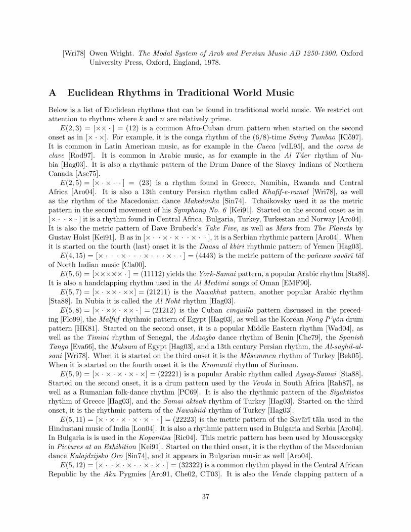
[Wri78] Owen Wright. The Modal System of Arab and Persian Music AD 1250-1300. OxfordUniversity Press, Oxford, England, 1978.
A Euclidean Rhythms in Traditional World Music
Below is a list of Euclidean rhythms that can be found in traditional world music. We restrict outattention to rhythms where k and n are relatively prime.
E(2, 3) = [×× · ] = (12) is a common Afro-Cuban drum pattern when started on the secondonset as in [× · ×]. For example, it is the conga rhythm of the (6/8)-time Swing Tumbao [Klo97].It is common in Latin American music, as for example in the Cueca [vdL95], and the coros declave [Rod97]. It is common in Arabic music, as for example in the Al Taer rhythm of Nu-bia [Hag03]. It is also a rhythmic pattern of the Drum Dance of the Slavey Indians of NorthernCanada [Asc75].
E(2, 5) = [× · × · · ] = (23) is a rhythm found in Greece, Namibia, Rwanda and CentralAfrica [Aro04]. It is also a 13th century Persian rhythm called Khafif-e-ramal [Wri78], as wellas the rhythm of the Macedonian dance Makedonka [Sin74]. Tchaikovsky used it as the metricpattern in the second movement of his Symphony No. 6 [Kei91]. Started on the second onset as in[× · · × · ] it is a rhythm found in Central Africa, Bulgaria, Turkey, Turkestan and Norway [Aro04].It is also the metric pattern of Dave Brubeck’s Take Five, as well as Mars from The Planets byGustav Holst [Kei91]. B as in [× · · × · × · · × · · ], it is a Serbian rhythmic pattern [Aro04]. Whenit is started on the fourth (last) onset it is the Daasa al kbiri rhythmic pattern of Yemen [Hag03].
E(4, 15) = [× · · · × · · · × · · · × · · ] = (4443) is the metric pattern of the pancam savarı talof North Indian music [Cla00].
E(5, 6) = [××××× · ] = (11112) yields the York-Samai pattern, a popular Arabic rhythm [Sta88].It is also a handclapping rhythm used in the Al Medemi songs of Oman [EMF90].
E(5, 7) = [× · ×× · ××] = (21211) is the Nawakhat pattern, another popular Arabic rhythm[Sta88]. In Nubia it is called the Al Noht rhythm [Hag03].
E(5, 8) = [× · ×× · ×× · ] = (21212) is the Cuban cinquillo pattern discussed in the preced-ing [Flo99], the Malfuf rhythmic pattern of Egypt [Hag03], as well as the Korean Nong P’yon drumpattern [HK81]. Started on the second onset, it is a popular Middle Eastern rhythm [Wad04], aswell as the Timini rhythm of Senegal, the Adzogbo dance rhythm of Benin [Che79], the SpanishTango [Eva66], the Maksum of Egypt [Hag03], and a 13th century Persian rhythm, the Al-saghil-al-sani [Wri78]. When it is started on the third onset it is the Musemmen rhythm of Turkey [Bek05].When it is started on the fourth onset it is the Kromanti rhythm of Surinam.
E(5, 9) = [× · × · × · × · ×] = (22221) is a popular Arabic rhythm called Agsag-Samai [Sta88].Started on the second onset, it is a drum pattern used by the Venda in South Africa [Rah87], aswell as a Rumanian folk-dance rhythm [PC69]. It is also the rhythmic pattern of the Sigaktistosrhythm of Greece [Hag03], and the Samai aktsak rhythm of Turkey [Hag03]. Started on the thirdonset, it is the rhythmic pattern of the Nawahiid rhythm of Turkey [Hag03].
E(5, 11) = [× · × · × · × · × · · ] = (22223) is the metric pattern of the Savarı tala used in theHindustani music of India [Lon04]. It is also a rhythmic pattern used in Bulgaria and Serbia [Aro04].In Bulgaria is is used in the Kopanitsa [Ric04]. This metric pattern has been used by Moussorgskyin Pictures at an Exhibition [Kei91]. Started on the third onset, it is the rhythm of the Macedoniandance Kalajdzijsko Oro [Sin74], and it appears in Bulgarian music as well [Aro04].
E(5, 12) = [× · · × · × · · × · × · ] = (32322) is a common rhythm played in the Central AfricanRepublic by the Aka Pygmies [Aro91, Che02, CT03]. It is also the Venda clapping pattern of a
37
South African children’s song [Pre83], and a rhythm pattern used in Macedonia [Aro04]. Startedon the second onset, it is the Columbia bell pattern popular in Cuba and West Africa [Klo97],as well as a drumming pattern used in the Chakacha dance of Kenya [Bar04b], and also used inMacedonia [Aro04]. Started on the third onset, it is the Bemba bell pattern used in NorthernZimbabwe [Pre83], and the rhythm of the Macedonian dance Ibraim Odza Oro [Sin74]. Started onthe fourth onset, it is the Fume Fume bell pattern popular in West Africa [Klo97], and is a rhythmused in the former Yugoslavia [Aro04]. Finally, when started on the fifth onset it is the Salve bellpattern used in the Dominican Republic in a rhythm called Canto de Vela in honor of the VirginMary [Far92], as well as the drum rhythmic pattern of the Moroccan Al Kudam [Hag03].
E(5, 13) = [× · · × · × · · × · × · · ] = (32323) is a Macedonian rhythm which is also played bystarting it on the fourth onset as follows: [× · × · · × · · × · × · · ] [Aro04].
E(5, 16) = [× · · × · · × · · × · · × · · · ] = (33334) is the Bossa-Nova rhythm necklace of Brazil.The actual Bossa-Nova rhythm usually starts on the third onset as follows: [× · · × · · × · · · × · ·× · · ] [Tou02]. However, other starting places are also documented in world music practices, suchas [× · · × · · × · · × · · · × · · ] [Beh73].
E(6, 7) = [×××××× · ] = (111112) is the Pontakos rhythm of Greece when started on the sixth(last) onset [Hag03].
E(6, 13) = [× · × · × · × · × · × · · ] = (222223) is the rhythm of the Macedonian dance MamaCone pita [Sin74]. Started on the third onset, it is the rhythm of the Macedonian dance PostupanoOro [Sin74], as well as the Krivo Plovdivsko Horo of Bulgaria [Ric04].
E(7, 8) = [××××××× · ] = (1111112), when started on the seventh (last) onset, is a typicalrhythm played on the Bendir (frame drum), and used in the accompaniment of songs of the Tuaregpeople of Libya [Sta88].
E(7, 9) = [× · ××× · ×××] = (2112111) is the Bazaragana rhythmic pattern of Greece [Hag03].E(7, 10) = [× · ×× · ×× · ××] = (2121211) is the Lenk fahhte rhythmic pattern of Turkey [Hag03].E(7, 12) = [× · ×× · × · ×× · × · ] = (2122122) is a common West African bell pattern. For
example, it is used in the Mpre rhythm of the Ashanti people of Ghana [Tou03]. Started on theseventh (last) onset, it is a Yoruba bell pattern of Nigeria, a Babenzele pattern of Central Africa,and a Mende pattern of Sierra Leone [Sto05].
E(7, 15) = [× · × · × · × · × · × · × · · ] = (2222223) is a Bulgarian rhythm when started on thethird onset [Aro04].
E(7, 16) = [× · · × · × · × · · × · × · × · ] = (3223222) is a Samba rhythm necklace from Brazil.The actual Samba rhythm is [× · × · · × · × · × · · × · × · ] obtained by starting E(7, 16) on thelast onset, and it coincides with a Macedonian rhythm [Aro04]. When E(7, 16) is started on thefifth onset it is a clapping pattern from Ghana [Pre83]. When it is started on the second onset itis a rhythmic pattern found in the former Yugoslavia [Aro04].
E(7, 17) = [× · · × · × · · × · × · · × · × · ] = (3232322) is a Macedonian rhythm when startedon the second onset [Sin74].
E(7, 18) = [× · · × · × · · × · × · · × · × · · ] = (3232323) is a Bulgarian rhythmic pattern [Aro04].E(8, 17) = [× · × · × · × · × · × · × · × · · ] = (22222223) is a Bulgarian rhythmic pattern which
is also started on the fifth onset [Aro04].E(8, 19) = [× · · × · × · × · · × · × · × · · × · ] = (32232232) is a Bulgarian rhythmic pattern
when started on the second onset [Aro04].E(9, 14) = [× · ×× · ×× · ×× · ×× · ] = (212121212), when started on the second onset, is the
rhythmic pattern of the Tsofyan rhythm of Algeria [Hag03].E(9, 16) = [× · ×× · × · × · ×× · × · × · ] = (212221222) is a rhythm necklace used in the Cen-
tral African Republic [Aro91]. When it is started on the second onset it is a bell pattern of the
38
Luba people of Congo [Mus02]. When it is started on the fourth onset it is a rhythm played in Westand Central Africa [Flo99], as well as a cow-bell pattern in the Brazilian samba [Sol96]. When it isstarted on the penultimate onset it is the bell pattern of the Ngbaka-Maibo rhythms of the CentralAfrican Republic [Aro91].
E(9, 22) =[× · · × · × · · × · × · · × · × · · × · × · ] = (323232322) is a Bulgarian rhythmic pat-tern when started on the second onset [Aro04].
E(9, 23) =[× · · × · × · · × · × · · × · × · · × · × · · ] = (323232323) is a Bulgarian rhythm [Aro04].E(11, 12) =[××××××××××× · ] = (11111111112), when started on the second onset, is the
drum pattern of the Rahmani (a cylindrical double-headed drum) used in the Sot silam dance fromMirbat in the South of Oman [EMF90].
E(11, 24) =[× · · × · × · × · × · × · · × · × · × · × · × · ] = (32222322222) is a rhythm necklaceof the Aka Pygmies of Central Africa [Aro91]. It is usually started on the seventh onset. Startedon the second onset, it is a Bulgarian rhythm [Aro04].
E(13, 24) =[× · ×× · × · × · × · × · ×× · × · × · × · × · ] = (2122222122222) is another rhythmnecklace of the Aka Pygmies of the upper Sangha [Aro91]. Started on the penultimate onset, it isthe Bobangi metal-blade pattern used by the Aka Pygmies.
E(15, 34) = [× · · × · × · × · × · · × · × · × · × · · × · × · × · × · · × · × · ] = (322232223222322)is a Bulgarian rhythmic pattern when started on the penultimate onset [Aro04].
39