the disappointing welfare impact of indirect pigouvian taxation
TRANSCRIPT
The Disappointing Welfare Impact of Indirect Pigouvian
Taxation: Evidence from Transportation
Christopher R. Knittel and Ryan Sandler∗
September 24, 2012
Abstract
A basic tenet of economics is that when consumers or firms don’t face the true social costof their actions, market outcomes are inefficient. In the case of negative externalities, Pigou-vian taxes are one way to correct this market failure, where the optimal tax leads agents tointernalize the true cost of their actions. A practical complication, however, is that the levelof externality nearly always varies across economic agents and directly taxing the externalitymay be infeasible. In such cases, policy often taxes a product correlated with the externality.For example, instead of taxing vehicle emissions directly, policy makers may tax gasoline eventhough per-gallon emissions vary across vehicles. This paper estimates the implications of thisapproach within the personal transportation market. We have three general empirical results.First, we show that vehicle emissions are positively correlated with vehicle elasticities for milestraveled with respect to fuel prices (in absolute value)—i.e. dirtier vehicles respond more to fuelprices. This correlation substantially increases the optimal second-best uniform gasoline tax.Second, and perhaps more importantly, we show that a uniform tax performs very poorly ineliminating deadweight loss associated with vehicle emissions; in many years in our sample over75 percent of the deadweight loss remains under the optimal second-best gasoline tax. Substan-tial improvements to market efficiency require differentiating based on vehicle type, for examplevintage. Finally, there is a more positive result: because of the positive correlation betweenemissions and elasticities, the health benefits from a given gasoline tax increase by roughly 90percent, compared to what one would expect if emissions and elasticities were uncorrelated.
∗This paper has benefited from conference discussion by Jim Sallee and conversations with Severin Borenstein,Joseph Doyle, Michael Greenstone, Michael Grubb, Jonathan Hughes, Dave Rapson, Nicholas Sanders, and CatherineWolfram. It has also benefited from participants at the NBER Energy and Environmental Economics Spring Meetingand seminar participants at Northeastern University, University of Chicago, MIT, and Yale University. We gratefullyacknowledge financial support from the University of California Center for Energy & Environmental Economics. Theresearch was also supported by a grant from the Sustainable Transportation Center at the University of CaliforniaDavis, which receives funding from the U.S. Department of Transportation and Caltrans, the California Department ofTransportation, through the University Transportation Centers program. The views expressed in this article are thoseof the authors and do not necessarily reflect those of the Federal Trade Commission. Knittel: William Barton RogersProfessor of Energy Economics, Sloan School of Management, MIT and NBER, email: [email protected]. Sandler:Federal Trade Commission, email: [email protected].
1 Introduction
A basic tenet of economics is that when consumers or firms do not face the true social cost
of their actions, market outcomes are inefficient. In the case of externalities, Pigouvian taxes
are one way to correct this market failure, and the optimal tax or subsidy leads agents to
internalize the true cost of their actions. A practical complication, however, is that the level
of externality nearly always varies across economic agents and directly taxing the externality
may be infeasible. In such cases, policy often taxes or subsidizes a product correlated with the
externality. For example, instead of taxing vehicle emissions directly, policy makers may tax
gasoline even though per-gallon emissions vary across vehicles. Similarly, a uniform alcohol or
tobacco tax is imposed as a means of reducing the negative externalities associated with their
use even though externalities may vary by person or alcohol type. Or, in the case of positive
externalities associated with research and development activities, policy might subsidize R&D
uniformly across firms.
In this paper, we address two related questions. The first is what is the size of the optimal
uniform tax rate for gasoline. The second is to what extent of the market inefficiency that
remains once this tax is imposed.
As to the first question, an obvious starting point for the optimal tax is to set a tax equal
to the average of the externality. Diamond (1973), however, shows that the correct tax is
based on the joint distribution of agent-specific externalities and demand elasticities. We
estimate this joint distribution and calculate how the two taxes differ.1
The second question we address has received very little attention in the literature, but is
perhaps even more important. Under the optimal uniform Pigouvian tax, deadweight loss will
remain, with some agents under-taxed and others over-taxed. The greater the heterogeneity,
the greater the deadweight loss that will remain. Understanding the efficiency gains of agent-
specific Pigouvian taxes relative to their uniform counterparts is a valuable input in the cost-
benefit analysis of policy makers. The larger is the remaining deadweight loss, the greater
the payoffs from taxing individuals differentially. Using the framework in Diamond (1973),
we analytically solve for the deadweight loss that remains. We then estimate the deadweight
1Parry and Small (2005) calculate the optimal tax based on average emissions given that the correlationbetween emissions and price responsiveness, as far as we are aware, has not been estimated.
1
loss that remains in our empirical setting.
Our empirical setting is the personal transportation market between 1998 and 2008. We
show three things.
First, we observe substantial variation in vehicle-level emissions (externalities) in the light-
duty vehicle market and that this variation is correlated with the vehicle-specific elasticity
of miles driven to gasoline prices. Dirtier vehicles are more price responsive. Using detailed
vehicle-specific data on miles driven, we show that that the positive correlation between
emissions and elasticities (in absolute value) hold for all three criteria pollutant emissions
for which we have data: carbon monoxide, hydrocarbons, and nitrogen oxides, as well as for
vehicle weight and greenhouse gases.2 We find that the average “two-year” elasticity of miles
traveled is -0.15 across all vehicles, but the the differences across vehicle types is substantial.
The elasticity for the dirtiest quartile of vehicles with respect to nitrogen oxides is -0.29. The
second, third and fourth quartile elasticities are -0.16, -0.06, and 0.04, respectively. Similar
variation exists for carbon monoxide and hydrocarbons. This correlation drives a wedge
between the optimal uniform Pigouvian tax associated with emissions and what we call the
“naive” tax which is based on average externalities. This increase is substantial, on the order
of 50 percent in each of the years of our sample (1998 to 2008).
Second, and we argue more importantly, even when instituting the optimal uniform Pigou-
vian tax, the uniform tax performs very poorly in eliminating deadweight loss. Across our
sample (1998 to 2008), we estimate that the optimal uniform Pigouvian tax, a gasoline tax
in this case, eliminates only 30 percent of the deadweight loss associated with these pollu-
tants. During the second half of our sample 75 percent of the deadweight loss remains under
the optimal uniform tax. We investigate ways to improve upon this. We find that allowing
gasoline taxes to be county specific leads to a small improvement, increasing the amount of
deadweight loss eliminated by less than 5 percentage points. We find moderate benefits from
“homogenizing” the fleet, potentially through vehicle retirement (“Cash-for-Clunkers) pro-
grams; scrapping the dirtiest 10 percent of vehicles reduces the deadweight loss that remains
2Criteria air pollutants are the only air pollutants for which the Administrator of the U.S. EnvironmentalProtection Agency has established national air quality standards defining allowable ambient air concentrations.Congress has focused regulatory attention on these pollutants (i.e., carbon monoxide, lead, nitrogen dioxide,ozone, particulate matter, and sulfur dioxide) because they endanger public health and they are widespreadthroughout the U.S..
2
by 14 percentage points. Only when taxes vary by vehicle type, e.g., vehicle’s age, do we see
a majority of the amount of deadweight loss eliminated.
Finally, there is some good news. We show that the positive correlation that we document
between emissions and the miles-driven elasticity (with respect to gasoline prices) implies that
health benefits from a given gasoline tax are larger than would be suggested by ignoring this
correlation. We estimate that across our sample, the health benefits of a gasoline tax, per
gallon of gasoline reduced, increase by 90 percent once one accounts for the the heterogeneity
that we document.
We also investigate several sources of the heterogeneity to the response of gasoline prices
on miles traveled. At the most general level, we show that while the age of the vehicle
contributes to our results—older vehicles respond more to changes in gasoline prices—this does
not explain all or even most of the heterogeneity. There are at least two additional sources of
criteria pollutant-related heterogeneity in the response of changes in gasoline prices. For one,
low income consumers may both own dirtier vehicles and be more responsive to changes in
gasoline prices. Second, the heterogeneity may come from within-household shifts in vehicle
miles traveled, for example if a household has one newer and one older vehicle. As gasoline
prices increase, they may shift miles away from the older vehicle and to the newer vehicle.
Because age is, on average, correlated with both fuel economy and criteria pollutant emissions,
this would lead to our result. Our data can speak to this. We find that while there is evidence
of both a within household effect and an income effect; but, a significant amount of variation
persists once these are accounted for.
We also estimate how the hazard rate of scrapping a vehicle varies with criteria pollutant
emissions. Here, the evidence is more mixed. We find little variation in scrappage across
emission levels within the same age. However, we find that increases in gasoline prices changes
the age distribution; older vehicles are scrapped sooner while middle-aged vehicles stay on
the road longer. Since older vehicles have higher levels of emissions, this too increases the
optimal uniform tax, but has a much smaller effect than the VMT variation.
An obvious concern is that our empirical results are only applicable to California. However,
in appendix D we present evidence that provided the heterogeneity is somewhat similar to
what we observe in California, the environmental benefits may be larger for other states.
The paper proceeds as follows. Section 2 draws on Diamond (1973) to derive the optimal
3
uniform gasoline tax and the amount of deadweight loss that remains. Section 3 discusses the
empirical setting. The data are discussed in Section 4. Section 5 provides graphical support
for the empirical results. Sections 6 and 7 present empirical models and results on miles driven
and scrappage. Section 8 estimates the empirically the optimal uniform tax and estimates
welfare effects, and Section 9 presents the results from our policy simulation. Finally, Section
10 concludes the paper.
2 Optimal Uniform Taxes
In this section, we derive the optimal uniform tax in the presence of heterogeneity in the
externality, following closely the model of Diamond (1973). We reiterate that the optimal
uniform Pigouvian tax is second best since heterogeneity would imply taxing different agents
differently.
Consumer h derives utility (indirectly, of course) from her gasoline purchases, αh, but is
also affected by the gasoline consumption of others, α−h. We assume single-car households
and discuss the robustness of these results after the formal model. Consumer h’s utility can
be written as:
Uh(α1, α2, ..., αh, ..., αn) + µh (1)
We assume utility is monotone in own consumption:
∂Uh
∂αh≥ 0. (2)
Consumers choose gasoline consumption to maximize utility. Formally we model this as
a quasi-linear utility function, given as:
maxαh
Uh(α1, α2, ..., αh, ..., αn) + µh, (3)
s.t. (p+ τ)αh + µh = mh. (4)
Where p is the price and τ the tax per gallon. Assuming an interior solution, we have:
∂Uh
∂αh= (p+ τ). (5)
4
This yields demand curves, given by:
α∗h = αh (p+ τ) . (6)
The optimal uniform Pigouvian tax will maximize social welfare, or the sum of utilities:
W (τ) =∑h
Uh[α∗1, ..., α∗h, ...α
∗n]− p
∑h
α∗h +∑h
mh. (7)
The first-order condition for the optimal uniform Pigouvian tax is given as:
W ′(τ) =∑h
∑i
∂Uh
∂αiα′i − p
∑h
α′h = 0. (8)
We can rewrite this as follows:
W ′(τ) =∑h
∑i 6=h
∂Uh
∂αiα′i +
∑h
∂Uh
∂αhα′h − p
∑h
α′h = 0, (9)
⇒ W ′(τ) =∑h
∑i 6=h
∂Uh
∂αiα′i +
∑h
α′h
(∂Uh
∂αh− p)
= 0. (10)
From the consumers’ first-order conditions, we have: ∂Uh
∂αh− p = τ . We can plug this in to
the social planner’s first-order condition to get:
W ′(τ) =∑h
∑i 6=h
∂Uh
∂αiα′i + τ
∑h
α′h = 0. (11)
Solving for the second-best tax yields:
τ ∗ =−∑
h
∑i 6=h
∂Uh
∂αiα′i∑
h α′h
. (12)
The optimal uniform Pigouvian tax becomes a weighted average of the vehicles’ external-
ities where the weights are the derivative of the externality with respect to the tax. There
are a few things to notice. First, the relative size of the optimal uniform Pigouvian tax and
the naive tax is unclear. The more price responsive are dirtier agents, or vehicles in our case,
the closer the tax will be to the marginal externality of these vehicles. However, if clean
vehicles are more sensitive than dirty vehicles, then the marginal externality is closer to the
externality of the clean vehicles.
5
As an intuitive example, imagine the case where there are only two vehicle types. The
first emits little pollution, while the second is dirtier. Also imagine the clean vehicles are
completely price insensitive, while the dirty vehicles are price sensitive. The naive Pigouvian
tax would tax based on the average emissions of the two vehicle types. However, the marginal
emission is the emission rate of the dirty vehicles; the clean cars are driven regardless of the
tax level. In this case, we can achieve first best by setting the tax rate at the externality rate
of the dirty vehicle. There is no distortion to owners of the clean vehicles since their demand
is completely inelastic, so we can completely internalize the externality to those driving the
dirty vehicles. The formula above implies this.
Second, as Diamond explicitly discusses, there is no requirement that all of the α′hs must
be negative, although the optimal second-best tax loses the interpretation as a weighted
average. Indeed, if households hold multiple vehicles, it is conceivable that miles traveled
is shifted from the low mileage vehicle to the high mileage vehicle. This also implies that
the second-best tax can be negative. For example, suppose the dirty vehicles had a positive
miles-traveled elasticity, while clean vehicles were very price sensitive. In this case, it may
be optimal for policy to subsidize gasoline. The trade-off being more miles from the cleaner
vehicles, but fewer miles traveled by the dirty ones. We will find, however, that the potential
for positive elasticities will drive the second-best tax upward; it can then exceed the negative
externality of the dirtiest vehicles.
Finally, the elasticity of the negative externality with respect to the price also accounts
for any changes on the extensive margin. That is, if the gasoline tax increases the scrappage
rate of some vehicles, then the relevant derivative of the externality with respect to price is
the expected change in miles driven, not the change in miles driven, conditional on survival.
The presence of heterogeneity also implies that the uniform tax will not achieve the first
best outcome. In short, the uniform tax will under-tax high externality agents and over-tax
low externality agents.
2.1 Extensions to Diamond (1973)
Diamond (1973) does not analyze the amount of deadweight loss remaining in the presence
of a uniform Pigouvian tax applied to a market with heterogenous externalities.
Suppose the drivers are homogenous in their demand for miles driven, but vehicles differ
6
in terms of emissions. In particular, each consumer has a demand for miles drive given as:
m = β0 − β1dpm(pg + τ). (13)
If the distribution of the externality per mile, E, is log normal, with probability density
function of:
ϕ(Ei) =1
Ei√
2σ2E
exp
(−(Ei − µE)2
2σ2E
). (14)
Given these assumptions, the deadweight loss absent any market intervention will be given
as:
D =
∫ ∞0
(Ei)2
2β1
ϕ(Ei)dEi
=1
2β1
E[E2i ] (15)
=1
2β1
e2µE+2σ2E .
Since the level of externality is uncorrelated with the slope of demand, the optimal uniform
Pigouvian tax will be the average emissions across all vehicles. This is given as:
E = τ = eµE+σ2E/2. (16)
The deadweight loss associated with all vehicles is given as:
D(τ) =
∫ ∞0
(τ − Ei)2
2β1
ϕ(Ei)dEi
=1
2β1
E[τ 2 − 2τEi + E2i ]
=1
2β1
(τ 2 − 2τE[Ei] + E[E2i ]) (17)
=1
2β1
(τ 2 − 2τeµE+σ2E2 + e2µE+2σ2
E)
=1
2β1
(τ 2 − 2τeµE+σ2E2 ) +D
= D − e2µE+σ2E
2β1
.
The ratio of the deadweight loss that remains with the deadweight loss absent the tax is
7
therefore:
R =D − e2µE+σ2E
2β1
D= 1− e2µE+σ2
E
e2µE+2σ2E
= 1− e−σ2E . (18)
With the externality uncorrelated with demand for miles driven, the remaining deadweight
loss from a uniform tax depends only on the shape parameter of the externality distribution.
The larger is σ2E, the wider and more skewed will be the distribution of the externality, causing
the uniform tax to “overshoot” the optimal quantity of miles for more vehicles.
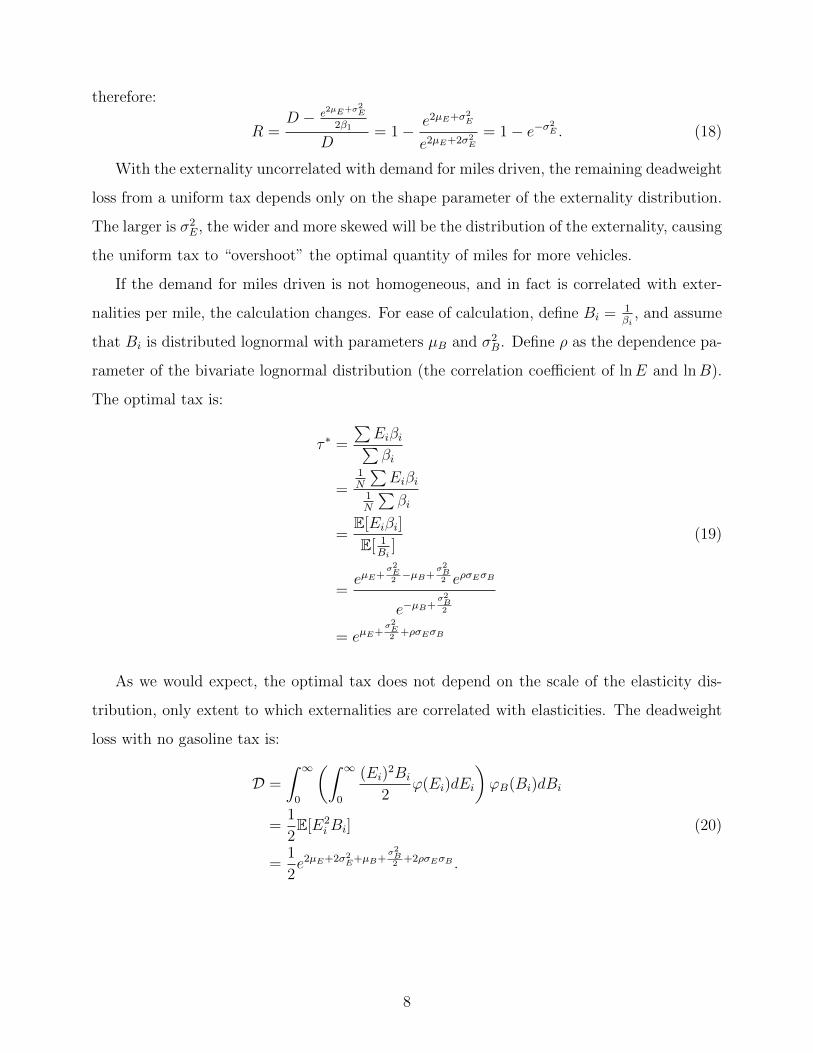
If the demand for miles driven is not homogeneous, and in fact is correlated with exter-
nalities per mile, the calculation changes. For ease of calculation, define Bi = 1βi
, and assume
that Bi is distributed lognormal with parameters µB and σ2B. Define ρ as the dependence pa-
rameter of the bivariate lognormal distribution (the correlation coefficient of lnE and lnB).
The optimal tax is:
τ ∗ =
∑Eiβi∑βi
=1N
∑Eiβi
1N
∑βi
=E[Eiβi]
E[ 1Bi
](19)
=eµE+
σ2E2−µB+
σ2B2 eρσEσB
e−µB+σ2B2
= eµE+σ2E2
+ρσEσB
As we would expect, the optimal tax does not depend on the scale of the elasticity dis-
tribution, only extent to which externalities are correlated with elasticities. The deadweight
loss with no gasoline tax is:
D =
∫ ∞0
(∫ ∞0
(Ei)2Bi
2ϕ(Ei)dEi
)ϕB(Bi)dBi
=1
2E[E2
iBi] (20)
=1
2e2µE+2σ2
E+µB+σ2B2
+2ρσEσB .
8
The deadweight loss with the optimal uniform tax is:
D(τ ∗) =
∫ ∞0
(∫ ∞0
(τ − Ei)2Bi
2ϕ(Ei)dEi
)ϕB(Bi)dBi
=1
2E[τ 2Bi − 2τEiBi + E2
iBi]
=1
2(τ 2E[Bi]− 2τE[EiBi] + E[E2
iBi]) (21)
=1
2(τ 2eµB+
σ2B2 − 2τeµE+
σ2E2
+µB+σ2B2
+ρσEσB + e2µE+2σ2E+µB+
σ2B2
+2ρσEσB)
=1
2e2µE+σ2
E+µB+σ2B2
+2ρσEσB − e2µE+σ2E+µB+
σ2B2
+2ρσEσB +D
= D − 1
2e2µE+σ2
E+µB+σ2B2
+2ρσEσB ,
while the deadweight loss with the naive tax, equal to the average externality level is:
D(τnaive) = D − 1
2(2e2µE+σ2
E+µB+σ2B2
+ρσEσB − e2µE+σ2E+µB+
σ2B2 ). (22)
Then the ratios of the remaining deadweight loss after a tax to the original deadweight
loss will be:
R(τ ∗) = 1− e2µE+σ2E+µB+
σ2B2
+2ρσEσB
e2µE+2σ2E+µB+
σ2B2
+2ρσEσB
= 1− e−σ2E , (23)
R(τnaive) = 1− 2e2µE+σ2E+µB+
σ2B2ρσEσB − e2µ+σ2
E+µB+σ2B2
e2µE+2σ2E+µB+
σ2B2
+2ρσEσB
= 1− e−σ2E(2e−ρσEσB − e−2ρσEσB). (24)
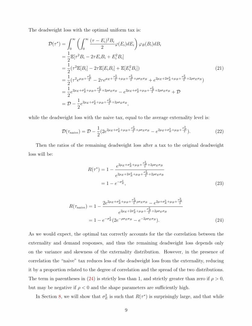
As we would expect, the optimal tax correctly accounts for the the correlation between the
externality and demand responses, and thus the remaining deadweight loss depends only
on the variance and skewness of the externality distribution. However, in the presence of
correlation the “naive” tax reduces less of the deadweight loss from the externality, reducing
it by a proportion related to the degree of correlation and the spread of the two distributions.
The term in parentheses in (24) is strictly less than 1, and strictly greater than zero if ρ > 0,
but may be negative if ρ < 0 and the shape parameters are sufficiently high.
In Section 8, we will show that σ2E is such that R(τ ∗) is surprisingly large, and that while
9
R(τnaive) is measurably larger, it is not much larger.
3 Empirical Setting
Our empirical setting is California. California implemented its first inspection and mainte-
nance program in 1984 in response to the 1977 Clean Air Act Amendments. The initial incar-
nation of the Smog Check program relied purely on a decentralized system of privately run,
state-licensed inspection stations, and was plagued by cheating and lax inspections. Although
the agreement between California and the federal EPA promised reductions in hydrocarbon
and carbon monoxide emissions of more the 25 percent, estimates of actual reductions of the
early Smog Check Program range from zero to half that amount (Glazer, Klein, and Lave
(1995)).
The 1990 Clean Air Act Amendments required states to implement an enhanced inspection
and maintenance program in areas with serious to extreme non-attainment of ozone limits.
Several of California’s urban areas fell into this category, and in 1994, a redesigned inspection
program was passed by California’s legislature after reaching a compromise with the EPA. The
program was updated in 1997 to address consumer complaints, and fully implemented by 1998.
Among other improvements, California’s new program introduced a system of centralized
“Test-Only” stations and an electronic transmission system for inspection reports.3 Today,
more than a million Smog Checks take place each month.
An automobile appears in the data for a number of reasons. First, vehicles that are older
than four years old must pass a smog check within 90 days of any change in ownership.
Second, in parts of the state (details below) an emissions inspection is required every other
year as a pre-requisite for renewing the registration on a vehicle that is six years old or older.
Third, a test is required if a vehicle moves from out-of-state. Vehicles which fail an inspection
must be repaired and receive another inspection before they can be registered and driven in
the state. There is also a group of exempt vehicles. These are: vehicles of 1975 model-year
or older, hybrid and electric vehicles, motorcycles, diesel powered vehicles, and large trucks
powered by natural gas.
Since 1998, the state has been divided into three inspection regimes (recently expanded
3For more detailed background see http://www.arb.ca.gov/msprog/smogcheck/july00/if.pdf.
10
to four), the boundaries of which roughly correspond to the jurisdiction of the regional Air
Quality Management Districts. “Enhanced” regions, designated because they fail to meet
state or federal standards for carbon monoxide (CO) and ozone, fall under the most restrictive
regime. All of the state’s major urban centers are in Enhanced areas, including the greater
Los Angeles, San Francisco, and San Diego metropolitan areas. Vehicles registered to an
address in an Enhanced area must pass a biennial Smog Check in order to be registered, and
they must take the more rigorous Acceleration Simulation Mode (ASM) test. The ASM test
involves the use of a dynamometer, and allows for measurement of NOx emissions. In addition,
a randomly selected two percent sample of all vehicles in these areas is directed to have their
Smog Checks at Test-Only stations, which are not allowed to make repairs.4 Vehicles which
match a “High Emitter Profile” are also directed to Test-Only stations, as are vehicles which
are flagged as “gross polluters” (this occurs when a vehicle fails an inspection with twice the
legal limit of one or more pollutant in its emissions). More recently some “Partial-Enhanced”
areas have been added, where a biennial ASM test is required, but no vehicles are directed to
Test-Only stations.
Areas with poor air quality that does not exceed legal limits fall under the Basic regime.
Cars in a Basic area must have biennial Smog Checks as part of registration, but they are
allowed to take the simpler Two Speed Idle (TSI) test, and no vehicles are directed to Test-
Only stations. The least restrictive regime, consisting of rural mountain and desert counties
in the east and north of the state, is known as the Change of Ownership area. As the name
suggests, inspections in these areas are only required upon change of ownership; no biennial
Smog Check is required.
3.1 Automobiles, Criteria Pollutants, and Health
The tests report the emissions of three criteria pollutant: Nitrogen oxides, hydrocarbon, and
carbon monoxide. All three of these pollutants are a direct consequences of the combustion
process within either gasoline or diesel engines. Both NOx and HCs are precursors to ground-
level ozone, but, as with CO, have been shown to have negative health effects individually.5
4Other vehicles can be taken to Test-Only stations as well if the owner chooses, although they must getrepairs elsewhere if they fail.
5CO has also been shown to speed up the smog-formation process. For early work on this, see Westberg,Cohen, and Wilson (1971).
11
While numerous studies have found links between the exposure of either smog or these
three pollutants directly and health outcomes, the direct mechanisms are still uncertain.
These pollutants, as well as smog, may directly impact vital organs or indirectly cause trauma.
For example, CO can bind to hemoglobin, thereby decreasing the amount of oxygen in the
bloodstream. High levels of carbon monoxide have also been linked to heart and respiratory
problems. NOx reacts with other compounds to create nitrate aerosols, which are fine-particle
particulate matter (PM). PM has been shown to irritate lung tissue, lowers lung capacity and
hinders long term-lung development. Extremely small PM can be absorbed through the lung
tissue and cause damage on the cellular level. On its own, HC can interfere with oxygen
intake and irritate lungs. Ground-level ozone is a known lung irritant, has been associated
with lowered lung capacity, and can exacerbate existing prior heart problems as well as lung
problems such as asthma or allergies.
4 Data
We bring together a number of large data sets. First, we have the universe of smog checks
from 1996 to 2010 from California’s Bureau of Automotive Repair (BAR). These data report
the location of the test, the vehicle’s VIN, odometer reading, the reason for the test, and test
results. We decode the VIN to obtain the vehicles’ make, model, engine, and transmission.
Using this, we match the vehicles to EPA data on fuel economy. Because the VIN decoding
only holds for vehicles made after 1981, our data are restricted to these models. We also
restrict our sample to 1998 and beyond given the large changes that occurred in the Smog
Check program in 1997. This yields roughly 120 million observations.
The Smog Check data report two measurements each nitrogen oxides and hydrocarbons
in terms of parts per million and carbon monoxide levels as a percentage of the exhaust,
taken under two engine speeds. As we are interested in the quantity of emissions, the more
relevant metric is a vehicles emissions per mile. We convert the smog check reading into
emissions per mile using conversion equations developed by Sierra Research for California Air
Resources Board for Morrow and Runkle (2005), an evaluation of the Smog Check program.
The conversion equations are functions of both measurements of all three pollutants, vehicle
weight, model year, and truck status.
12
We also estimate scrappage decisions. For this we use data reported to CARFAX Inc. for
32 million of the vehicles in the BAR data. These data contain the date and location of the
last record reported to CARFAX. This includes registrations, emissions inspections, repairs,
import/export records and accidents.
At times we use information about the household. For a subsample of our BAR data, we are
able to match vehicles to given households using data come from confidential Department of
Motor Vehicle records that track the registered address of the vehicle. We use this information
to aggregate up to addresses, the stock of vehicles registered. Appendix A discusses how this
is done. These data are from 2000 to 2008.
Finally, we use gasoline prices from EIA’s weekly California average price series to con-
struct average prices between Smog Check.
Table 1 reports means and standard deviations of the main variables used in our analysis,
as well as these summary statistics split by vehicle vintage and 1998 and 2008. The average
fuel economy of vehicles in our sample is 23.5 MPG, with fuel economy falling over our
sample. The change in the average dollar per mile has been dramatic, more than doubling
over our sample. The dramatic decrease in vehicle emissions is also clear in the data, with
per-mile emissions of hydrocarbon, CO, and NOx falling considerable from 1998 to 2008. The
tightening of standards has also meant that more vehicles fail the smog check late in the
sample, although some of this is driven by the aging vehicle fleet.
5 Preliminary Evidence
One of the main driving forces behind our empirical results is whether vehicle elasticities, both
in terms of their intensive and extensive margins, vary systematically with the magnitude
of their externalities. In this section, we present evidence that significant variation exists in
terms of vehicle externalities within a year, across years, and even within the same vehicle type
(make, model, model year, etc.) within a year. Further, simple statistics, such as the average
miles traveled by vehicle type, suggest that elasticities are correlated with externalities.6
Figure 1 plots the distributions of NOx, HCs, and CO emissions in 1998, 2004, and 2010.
The distribution of criteria pollutant emissions tends to be right-skewed in any given year,
6We are not the first to document the large variation across vehicles in emissions. See, for example, Kahn(1996). Instead, the contribution is in finding a link between elasticities and emissions.
13
with a standard deviation equal to roughly one to three times the mean, depending on the
pollutant. This implies that there are a vehicles on the road that are quite “dirty” relative
to the mean vehicle. Over time, the distribution has shifted to the left, as vehicles have been
getting cleaner, but the range still remains.
Table 2 reports the means and standard deviations across all vehicles receiving smog checks
in a given year. From 1998 to 2008 the average emissions of NOx, HCs, and CO fell between
65 and 85 percent. However, the standard deviations, relative to the means, have increased
over time. This is especially true for CO, where the standard deviation is over 4 times the
mean at the end of the sample.
This variation is not only driven by the fact that different types of vehicles are on the road
in a given year, but also variation within the same vehicle type, defined as a make, model,
model-year, engine, number of doors, and drivetrain combination. To see this, Figure 2 plots
the distributions of emissions for the most popular vehicle/year in our sample, the 2001 4-door
Toyota Corolla in 2009. The vertical red line is at the mean of the distribution. Here, again,
we see that even within the same vehicle-type in the same year, the distribution is wide and
right skewed. The distribution of hydrocarbons is less skewed, but the standard deviation is
25 percent of the mean. Carbon monoxide is also less skewed, and has a standard deviation
that is 36 percent of the mean. Across all years and vehicles, the mean emission rate of a
given vehicle in a given year, on average, is roughly four times the standard deviation for all
three pollutants (Table 2).
To understand how the distribution within a given vehicle changes over time, Figure 3
plots the distribution of the 1995 3.8L, front-wheel drive, Ford Windstar in 1999, 2001, 2004,
and 2007.7 These figures suggest that over time the distributions shift to the right, become
more symmetric, and the standard deviation grows considerably, relative to the mean. Across
all vehicles, the ratio of the mean emission rate of NOx and the standard deviation of NOx
has increased from 3.16 in 1998 to 4.53 in 2010. For hydrocarbons, this has increased from
3.59 to 5.51; and, has increased from 3.95 to 5.72 for CO.
These distributions demonstrate that there is significant variation in emissions across
vehicles and within vehicle type, and thus significant scope for meaningful emissions-correlated
7We chose this vehicle because the 1995 3.8L, front-wheel drive, Ford Windstar in 1999 is the second mostpopular entry in our data and it is old enough that we can track it over four 2-year periods.
14
variation in elasticities along those lines. We next present suggestive evidence that this is the
case. To do this, we categorize vehicles into four groups, based on the four quartiles of a given
pollutant within a given year. We then plot how the log of daily miles driven has changed
over our sample—a period where gasoline prices increased from roughly $1.35 to $3.20.
Figure 4 and 5 foreshadow our results on the intensive margin. Figure 4 plots the median
of daily miles traveled across our sample split up by the emissions quartile of the vehicle.
While the dirtiest quartile begins at a slightly lower daily-VMT, it appears to drop much
further than the other quartiles. Indeed, the there is a general trend of monotonicity across
the four emissions. To see this more clearly, Figure 5 rescales the median VMT in 1998
and plots the average of the log of VMT over time by quartiles of each pollutant. For each
pollutant, the log change in bottom-quartile vehicles is larger than the first quartile, with the
other two quartiles often exhibiting monotonic changes in miles driven.
6 Vehicle Miles Traveled Decisions
Our first set of empirical models estimates how vehicle miles traveled (VMT) decisions are
affected by changes in gasoline prices, and how this elasticity varies with vehicle character-
istics. Our empirical approach mirrors Figures 4 to 5. For each vehicle receiving a biennial
smog check, we calculate average daily miles driven and the average gasoline price during the
roughly two years between smog checks. We will then allow the elasticity to vary based on
the emissions of the vehicle. We begin by estimating:
ln(VMTijgt) = β ln(DPMijgt) + γDtruck + ωtime+ µt + µj + µg + µv + εigt (25)
where i indexes vehicles, j vehicle-types, g geographic locations, t time, and v vehicle age, or
vintage. DPMijgt is the average dollars per mile of the vehicle between smog checks, Dtruck
is an indicator for whether the vehicle is a truck, and time is a time trend.8
Table 3 shows our basic results. Model 1 controls only for year and vintage fixed effects,
with zip-code level demographic characteristics, and indicates and elasticity of -0.265. Simply
including make fixed effects in model 2 reduces this to -0.117. Model 3 also includes make
8Our dollars per mile variable uses the standard assumption that 45 percent of a vehicle miles driven arein the city and 55 percent are on the highway, along with the vehicles EPA fuel economy ratings.
15
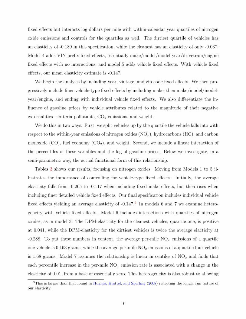
fixed effects but interacts log dollars per mile with within-calendar year quartiles of nitrogen
oxide emissions and controls for the quartiles as well. The dirtiest quartile of vehicles has
an elasticity of -0.189 in this specification, while the cleanest has an elasticity of only -0.037.
Model 4 adds VIN-prefix fixed effects, essentially make/model/model year/drivetrain/engine
fixed effects with no interactions, and model 5 adds vehicle fixed effects. With vehicle fixed
effects, our mean elasticity estimate is -0.147.
We begin the analysis by including year, vintage, and zip code fixed effects. We then pro-
gressively include finer vehicle-type fixed effects by including make, then make/model/model-
year/engine, and ending with individual vehicle fixed effects. We also differentiate the in-
fluence of gasoline prices by vehicle attributes related to the magnitude of their negative
externalities—criteria pollutants, CO2 emissions, and weight.
We do this in two ways. First, we split vehicles up by the quartile the vehicle falls into with
respect to the within-year emissions of nitrogen oxides (NOx), hydrocarbons (HC), and carbon
monoxide (CO), fuel economy (CO2), and weight. Second, we include a linear interaction of
the percentiles of these variables and the log of gasoline prices. Below we investigate, in a
semi-parametric way, the actual functional form of this relationship.
Tables 3 shows our results, focusing on nitrogen oxides. Moving from Models 1 to 5 il-
lustrates the importance of controlling for vehicle-type fixed effects. Initially, the average
elasticity falls from -0.265 to -0.117 when including fixed make effects, but then rises when
including finer detailed vehicle fixed effects. Our final specification includes individual vehicle
fixed effects yielding an average elasticity of -0.147.9 In models 6 and 7 we examine hetero-
geneity with vehicle fixed effects. Model 6 includes interactions with quartiles of nitrogen
oxides, as in model 3. The DPM-elasticity for the cleanest vehicles, quartile one, is positive
at 0.041, while the DPM-elasticity for the dirtiest vehicles is twice the average elacticity at
-0.288. To put these numbers in context, the average per-mile NOx emissions of a quartile
one vehicle is 0.163 grams, while the average per-mile NOx emissions of a quartile four vehicle
is 1.68 grams. Model 7 assumes the relationship is linear in centiles of NOx and finds that
each percentile increase in the per-mile NOx emission rate is associated with a change in the
elasticity of .001, from a base of essentially zero. This heterogeneity is also robust to allowing
9This is larger than that found in Hughes, Knittel, and Sperling (2008) reflecting the longer run nature ofour elasticity.
16
our other covariates to vary with NOx quartiles, and to employing a log-linear specification
with the level of dollars miles as the variable of interest; see appendix Tables A.23 and A.24.
We find similar patterns across the other externalities. Table 4 gives the DPM elasticities
by quartile for each of the five externalities. There is slightly more heterogeneity over hydro-
carbon and carbon monoxide emissions than over nitrogen oxides, with the dirtiest quartiles
around -0.31 and the cleanest around -0.5. For CO2 the cleanest vehicles are those with the
highest fuel economy, and here we see the least fuel-efficient vehicles having an elasticity of
-0.188, compared to -0.108. We observe some heterogeneity over weight as well, although it
is smaller than the other externalities.
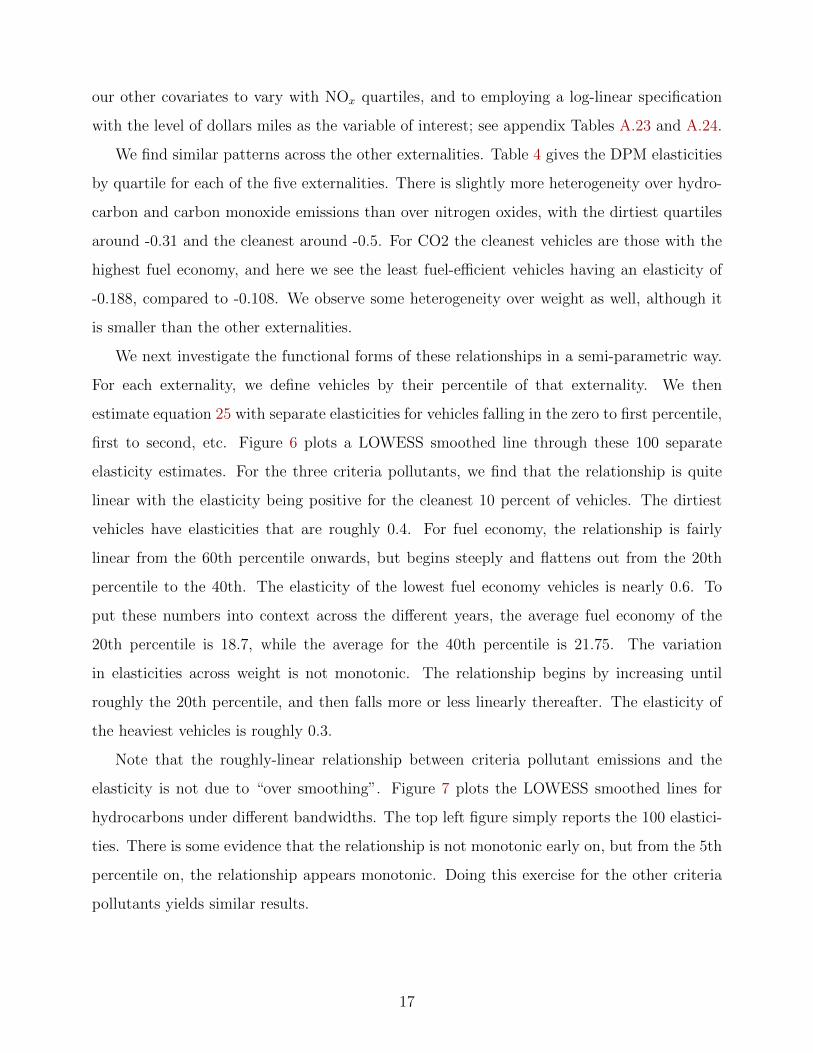
We next investigate the functional forms of these relationships in a semi-parametric way.
For each externality, we define vehicles by their percentile of that externality. We then
estimate equation 25 with separate elasticities for vehicles falling in the zero to first percentile,
first to second, etc. Figure 6 plots a LOWESS smoothed line through these 100 separate
elasticity estimates. For the three criteria pollutants, we find that the relationship is quite
linear with the elasticity being positive for the cleanest 10 percent of vehicles. The dirtiest
vehicles have elasticities that are roughly 0.4. For fuel economy, the relationship is fairly
linear from the 60th percentile onwards, but begins steeply and flattens out from the 20th
percentile to the 40th. The elasticity of the lowest fuel economy vehicles is nearly 0.6. To
put these numbers into context across the different years, the average fuel economy of the
20th percentile is 18.7, while the average for the 40th percentile is 21.75. The variation
in elasticities across weight is not monotonic. The relationship begins by increasing until
roughly the 20th percentile, and then falls more or less linearly thereafter. The elasticity of
the heaviest vehicles is roughly 0.3.
Note that the roughly-linear relationship between criteria pollutant emissions and the
elasticity is not due to “over smoothing”. Figure 7 plots the LOWESS smoothed lines for
hydrocarbons under different bandwidths. The top left figure simply reports the 100 elastici-
ties. There is some evidence that the relationship is not monotonic early on, but from the 5th
percentile on, the relationship appears monotonic. Doing this exercise for the other criteria
pollutants yields similar results.
17
6.1 The Source of the Heterogeneity
While the optimal uniform Pigouvian tax is not affected by the mechanism behind the het-
erogeneity, it is of independent interest to investigate the mechanism. We investigate three
sources, which are not necessarily independent of each other. First, it may be driven entirely
through a vintage effect. That is, older vehicles are both more responsive to changes in gaso-
line prices and have higher emissions. Second, it might be driven by differences in the incomes
of consumers that drive dirtier versus cleaner vehicles.10 Third, it may result from households
shifting which of their vehicles are driven in the face of rising gasoline prices.
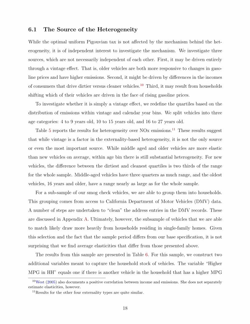
To investigate whether it is simply a vintage effect, we redefine the quartiles based on the
distribution of emissions within vintage and calendar year bins. We split vehicles into three
age categories: 4 to 9 years old, 10 to 15 years old, and 16 to 27 years old.
Table 5 reports the results for heterogeneity over NOx emissions.11 These results suggest
that while vintage is a factor in the externality-based heterogeneity, it is not the only source
or even the most important source. While middle aged and older vehicles are more elastic
than new vehicles on average, within age bin there is still substantial heterogeneity. For new
vehicles, the difference between the dirtiest and cleanest quartiles is two thirds of the range
for the whole sample. Middle-aged vehicles have three quarters as much range, and the oldest
vehicles, 16 years and older, have a range nearly as large as for the whole sample.
For a sub-sample of our smog check vehicles, we are able to group them into households.
This grouping comes from access to California Department of Motor Vehicles (DMV) data.
A number of steps are undertaken to “clean” the address entries in the DMV records. These
are discussed in Appendix A. Ultimately, however, the subsample of vehicles that we are able
to match likely draw more heavily from households residing in single-family homes. Given
this selection and the fact that the sample period differs from our base specification, it is not
surprising that we find average elasticities that differ from those presented above.
The results from this sample are presented in Table 6. For this sample, we construct two
additional variables meant to capture the household stock of vehicles. The variable “Higher
MPG in HH” equals one if there is another vehicle in the household that has a higher MPG
10West (2005) also documents a positive correlation between income and emissions. She does not separatelyestimate elasticities, however.
11Results for the other four externality types are quite similar.
18
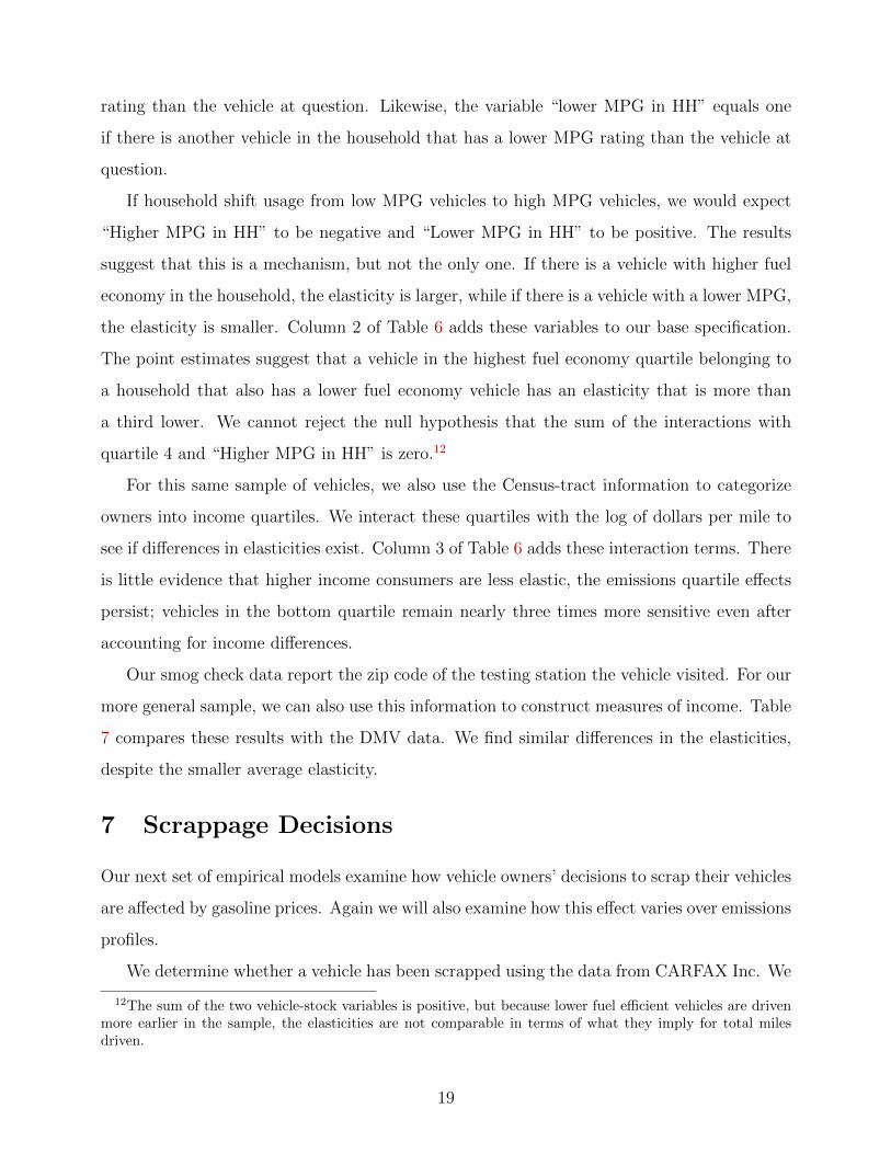
rating than the vehicle at question. Likewise, the variable “lower MPG in HH” equals one
if there is another vehicle in the household that has a lower MPG rating than the vehicle at
question.
If household shift usage from low MPG vehicles to high MPG vehicles, we would expect
“Higher MPG in HH” to be negative and “Lower MPG in HH” to be positive. The results
suggest that this is a mechanism, but not the only one. If there is a vehicle with higher fuel
economy in the household, the elasticity is larger, while if there is a vehicle with a lower MPG,
the elasticity is smaller. Column 2 of Table 6 adds these variables to our base specification.
The point estimates suggest that a vehicle in the highest fuel economy quartile belonging to
a household that also has a lower fuel economy vehicle has an elasticity that is more than
a third lower. We cannot reject the null hypothesis that the sum of the interactions with
quartile 4 and “Higher MPG in HH” is zero.12
For this same sample of vehicles, we also use the Census-tract information to categorize
owners into income quartiles. We interact these quartiles with the log of dollars per mile to
see if differences in elasticities exist. Column 3 of Table 6 adds these interaction terms. There
is little evidence that higher income consumers are less elastic, the emissions quartile effects
persist; vehicles in the bottom quartile remain nearly three times more sensitive even after
accounting for income differences.
Our smog check data report the zip code of the testing station the vehicle visited. For our
more general sample, we can also use this information to construct measures of income. Table
7 compares these results with the DMV data. We find similar differences in the elasticities,
despite the smaller average elasticity.
7 Scrappage Decisions
Our next set of empirical models examine how vehicle owners’ decisions to scrap their vehicles
are affected by gasoline prices. Again we will also examine how this effect varies over emissions
profiles.
We determine whether a vehicle has been scrapped using the data from CARFAX Inc. We
12The sum of the two vehicle-stock variables is positive, but because lower fuel efficient vehicles are drivenmore earlier in the sample, the elasticities are not comparable in terms of what they imply for total milesdriven.
19
begin by assuming that a vehicle has been scrapped if more than a year has passed between
the last record reported to CARFAX and the date when CARFAX produced our data extract
(October 1, 2010). However, we treat a vehicle as being censored if the last record reported
to CARFAX was not in California, or if more than a year and a half passed between the last
Smog Check in our data and that last record. As well, to avoid treating late registrations as
scrappage, we treat all vehicles with Smog Checks after 2008 as censored. Finally, to be sure
we are dealing with scrapping decisions and not accidents or other events, we only examine
vehicles which are at least 10 years old.
Some modifications to our data are necessary. To focus on the long-run response to
gasoline prices, our model is specified in discrete time, denominated in years. Where vehicles
have more than one Smog Check per calendar year, we use the last Smog Check in that year.
Also, since it is generally unlikely that a vehicle is scrapped at the same time as its last Smog
Check, we create an additional observation for scrapped vehicles either one year after the
last Smog Check, or 6 months after the last CARFAX record, whichever is later. For these
created observations, odometer is imputed based on the average VMT between the last two
Smog Checks, and all other variables take their values from the vehicle’s last Smog Check.
An exception is if a vehicle fails the last Smog Check in our data. In this case, we assume the
vehicle was scrapped by the end of that year.
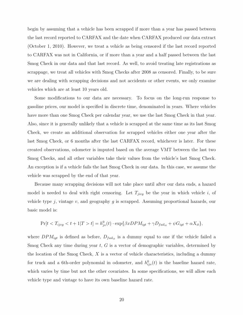
Because many scrapping decisions will not take place until after our data ends, a hazard
model is needed to deal with right censoring. Let Tjivg be the year in which vehicle i, of
vehicle type j, vintage v, and geography g is scrapped. Assuming proportional hazards, our
basic model is:
Pr[t < Tijvg < t+ 1|T > t] = h0jv(t) · exp{βxDPMigt + γDfailit + ψGigt + αXit},
where DPMigt is defined as before, Dfailit is a dummy equal to one if the vehicle failed a
Smog Check any time during year t, G is a vector of demographic variables, determined by
the location of the Smog Check, X is a vector of vehicle characteristics, including a dummy
for truck and a 6th-order polynomial in odometer, and h0ijv(t) is the baseline hazard rate,
which varies by time but not the other covariates. In some specifications, we will allow each
vehicle type and vintage to have its own baseline hazard rate.
20
We estimate this model using semi-parametric Cox proportional hazards regressions, leav-
ing the baseline hazard unspecified. We report exponentiated coefficients, which may be
interpreted as hazard ratios. For instance, a 1 unit increase in DPM will multiply the hazard
rate by exp{β}, or increase it by (exp{β} − 1) percent. In practice, we scale the coefficients
on DPM for a 5-cent change, corresponding to a $1.00 increase in gasoline prices for a vehicle
with fuel economy of 20 miles per gallon.
Tables 8 and 9 show the results of our hazard analysis. Models 1 and 2 of table 8 assign
all vehicles to the same baseline hazard function. Model 1 allows the effect of gasoline prices
to vary by whether or not a vehicle failed a Smog Check. Model 2 also allows the effect
of gasoline prices to vary by quartiles of NOx as well.13 Models 3 and 4 are similar, but
stratify the baseline hazard function, allowing each VIN prefix to have its own baseline hazard
function. Model 5 allows the effect of gasoline prices to vary both by externality quartile and
age group, separating vehicles 10 to 15 years old from vehicles 16 years and older.
Models 1 and 2 indicate that increases in gasoline prices actually decrease scrapping on
average, with the cleanest vehicles seeing the largest decreases. The effect is diminished
once unobserved heterogeneity among vehicle types is controlled for, but is still statistically
significant. However, the true heterogeneity in the effect of gasoline prices on hazard seems
to be over age groups. Model 5 shows that when the cost of driving a mile increases by 5
cents, the hazard of scrappage decreases by about 23% for vehicles between 10 and 15 years
old, while it increases by around 3% for vehicles age 16 and older, with little variation across
NOx quartiles within age groups. This suggests that when gasoline prices rise, very old cars
are scrapped, increasing demand for moderately old cars and thus reducing the chance that
they are scrapped.
Table 9 presents the quartile by age by dollars per mile interactions for each of the 5
externality dimensions. Hydrocarbons and carbon monoxide have the identical pattern to
NOx, with no heterogeneity within age-group. With fuel economy and vehicle weight, there is
within-age heterogeneity, although the form is counter-intuitive. The heaviest and least fuel
efficient vehicles are relatively less likely to be scrapped when gasoline prices increase than
the lightest and most fuel efficient. That is, while all 10–15 year old vehicles are less likely
13Quartiles in these models are calculated by year among only vehicles 10 years and older.
21
to be scrapped, the decrease in hazard rate is larger for heavy, gas-guzzling vehicles. For
vehicles 16 years and older, the heaviest quartile is less likely to be scrapped when gasoline
prices increase, even though the lightest (and middle quartiles) are more likely. As the model
stratifies by VIN prefix, this cannot be simply that more durable vehicles have lower fuel
economy.
In summary, increases in the cost of driving a mile over the long term increase the chance
that old vehicles are scrapped, while middle aged vehicles are scrapped less, perhaps because
of increased demand. Although vehicle age is highly correlated with emissions of criteria
pollutants, there is little variation in the response to gasoline prices across emissions rates
within age groups.
8 Efficiency of Uniform Pigouvian Taxes
In this section, we consider the efficiency of using a uniform Pigouvian tax to abate the
externalities caused by driving, specifically those resulting from emissions of NOx, HCs and
CO. We will begin by calculating both the “naive” and optimal second-best Pigouvian tax,
and then compare the remaining dead weight loss left over from these second-best taxes to
the optimal outcome obtained by a vehicle specific tax.
8.1 Optimal Uniform Pigouvian Tax
We calculate the “naive” Pigouvian tax per gallon of gasoline as the simple average of the
externality per gallon caused by all vehicles on the road in California in a particular year.
We value the externalities imposed by NOx and HCs using the marginal damages calculated
by Muller and Mendelsohn (2009), based on the county each vehicle has its Smog Check in.14
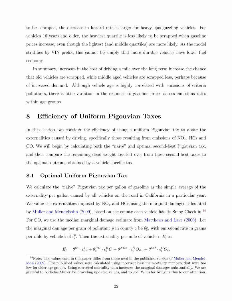
For CO, we use the median marginal damage estimate from Matthews and Lave (2000). Let
the marginal damage per gram of pollutant p in county c be θpc , with emissions rate in grams
per mile by vehicle i of εpi . Then the externality per mile of vehicle i, Ei is:
Ei = θhc · εhi c+ θHCc · εHi C + θNOx · εNi Oxc + θCO · εCi Oc.
14Note: The values used in this paper differ from those used in the published version of Muller and Mendel-sohn (2009). The published values were calculated using incorrect baseline mortality numbers that were toolow for older age groups. Using corrected mortality data increases the marginal damages substantially. We aregrateful to Nicholas Muller for providing updated values, and to Joel Wiles for bringing this to our attention.
22
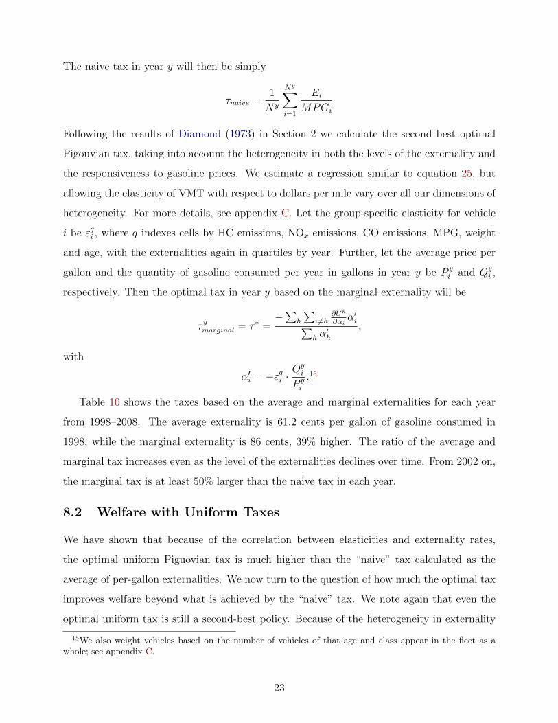
The naive tax in year y will then be simply
τnaive =1
Ny
Ny∑i=1
EiMPGi
Following the results of Diamond (1973) in Section 2 we calculate the second best optimal
Pigouvian tax, taking into account the heterogeneity in both the levels of the externality and
the responsiveness to gasoline prices. We estimate a regression similar to equation 25, but
allowing the elasticity of VMT with respect to dollars per mile vary over all our dimensions of
heterogeneity. For more details, see appendix C. Let the group-specific elasticity for vehicle
i be εqi , where q indexes cells by HC emissions, NOx emissions, CO emissions, MPG, weight
and age, with the externalities again in quartiles by year. Further, let the average price per
gallon and the quantity of gasoline consumed per year in gallons in year y be P yi and Qy
i ,
respectively. Then the optimal tax in year y based on the marginal externality will be
τ ymarginal = τ ∗ =−∑
h
∑i 6=h
∂Uh
∂αiα′i∑
h α′h
,
with
α′i = −εqi ·Qyi
P yi
.15
Table 10 shows the taxes based on the average and marginal externalities for each year
from 1998–2008. The average externality is 61.2 cents per gallon of gasoline consumed in
1998, while the marginal externality is 86 cents, 39% higher. The ratio of the average and
marginal tax increases even as the level of the externalities declines over time. From 2002 on,
the marginal tax is at least 50% larger than the naive tax in each year.
8.2 Welfare with Uniform Taxes
We have shown that because of the correlation between elasticities and externality rates,
the optimal uniform Piguovian tax is much higher than the “naive” tax calculated as the
average of per-gallon externalities. We now turn to the question of how much the optimal tax
improves welfare beyond what is achieved by the “naive” tax. We note again that even the
optimal uniform tax is still a second-best policy. Because of the heterogeneity in externality
15We also weight vehicles based on the number of vehicles of that age and class appear in the fleet as awhole; see appendix C.
23
levels, the most polluting vehicles will be taxed by less than their external costs to society,
leaving remaining dead weight loss. Vehicles which are cleaner than the weighted average
will be taxed too much, overshooting the optimal quantity of consumption and creating more
deadweight loss—potentially more than those vehicle contributed prior to the tax.
In each of the following analyses, we compare the remaining deadweight loss resulting from
the local pollution externality with each tax to the deadweight loss without any additional
tax.
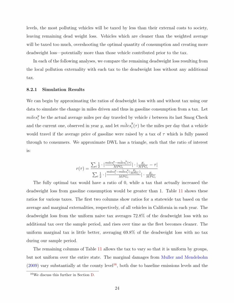
8.2.1 Simulation Results
We can begin by approximating the ratios of deadweight loss with and without tax using our
data to simulate the change in miles driven and thus in gasoline consumption from a tax. Let
milesyi be the actual average miles per day traveled by vehicle i between its last Smog Check
and the current one, observed in year y, and let ˆmilesy
i (τ) be the miles per day that a vehicle
would travel if the average price of gasoline were raised by a tax of τ which is fully passed
through to consumers. We approximate DWL has a triangle, such that the ratio of interest
is:
r(τ) =
∑i
12· |miles
yi− ˆmiles
yi (τ)
MPGi| · | Ei
MPGi− τ |∑
i12· |milesyi− ˆmiles
yi (
EiMPGi
)
MPGi| · Ei
MPGi
The fully optimal tax would have a ratio of 0, while a tax that actually increased the
deadweight loss from gasoline consumption would be greater than 1. Table 11 shows these
ratios for various taxes. The first two columns show ratios for a statewide tax based on the
average and marginal externalities, respectively, of all vehicles in California in each year. The
deadweight loss from the uniform naive tax averages 72.8% of the deadweight loss with no
additional tax over the sample period, and rises over time as the fleet becomes cleaner. The
uniform marginal tax is little better, averaging 69.8% of the deadweight loss with no tax
during our sample period.
The remaining columns of Table 11 allows the tax to vary so that it is uniform by groups,
but not uniform over the entire state. The marginal damages from Muller and Mendelsohn
(2009) vary substantially at the county level16, both due to baseline emissions levels and the
16We discuss this further in Section D.
24
population exposed to harmful emissions. As such, a county-specific tax on emissions might
be expected to target externality levels more precisely. The third and fourth columns of Table
11 shows the deadweight loss ratios for an average and marginal tax computed this way, and it
turns out there is relatively little improvement. The average ratios over our sample are 0.684
for and average tax and 0.653 for a marginal tax. Since emissions rates are highly correlated
with vintage, another approach would be to tax the average or marginal externality rate
by age. The fifth and sixth columns of the table show this, and here we see a substantial
improvement: 0.342 for the naive tax and 0.34 for a marginal tax. Combining these and
having the tax vary by both vintage and location, shown in the last two columns, reduces the
ratios to 0.276 and 0.274, respectively.
This analysis shows two striking results. First, a uniform Pigouvian tax does a terrible job
of addressing the market failure from the pollution externality. The dirtiest vehicles are not
taxed enough, and many clean vehicles are over taxed. This is true even when the uniform
tax is calculated taking heterogeneity into account. The roughly 50% increase in the tax
level from a marginal tax correctly abates more emissions from the dirtiest vehicles, but also
over-taxes the cleanest vehicles by a larger amount. This is still an improvement over the
naive tax, but not by much. The number of vehicles for which the uniform tax overshoots is
striking. Table 12 shows the proportion of vehicle-years over the 11 years of our sample for
which each tax overshoots. Because the distribution of emissions is so strongly right skewed,
the naive uniform tax overshoots more than 72% of the time, and the optimal uniform tax
by even more. Second, there is enough heterogeneity in the distribution of the per-gallon
externality that even a targetted tax that targets broad groups leaves a substantial portion
of the deadweight loss. Overshooting is again an issue—when the tax is allowed to vary by
county and vintage, only the average tax by county and vintage overshoots for less than 70%
of vehicles.
The variance and skewness in the distribution of externality per gallon causes a uniform
tax to be less efficient than might otherwise be expected. Figure 8 shows this clearly, plotting
the kernel density of the externality per gallon in 1998 and 2008, with vertical lines indicating
the naive tax and the optimal tax, respectively. The long right tail of the distribution requires
that either tax be much higher than the median externality.
We next examine how the optimal uniform tax would compare to the optimal vehicle
25
specific tax if the distribution become less skewed. That is, how would a uniform tax perform
if the right tail of the distribution—the oldest, dirtiest vehicles—were removed from the road?
This could be achieved directly from a “cash for clunkers”-style program, or indirectly through
tightening emissions standards in the Smog Check Program. Sandler (Forthcoming) shows
that vehicle retirement programs are not a cost-effective way to reduce criteria emissions, and
possibly grossly over pay for emissions, but the overall welfare consequences of this sort of
scheme may be more favorable if they improve the efficiency of a uniform gasoline tax. Table
13 shows the ratios of the deadweight loss with the optimal Pigouvian tax to the deadweight
loss with no tax, with increasing proportions of the top of the externality distribution removed.
Removing the top 1% increases the DWL reduction from 30% to 38% of the total with no
tax. Scrapping more of the top end of the distribution improves things further. If the most
polluting 25% of vehicles were removed from the road and the optimal Pigouvian tax was
imposed based on the weighted externality of the remaining 75%, this would remove 58.3%
of remaining deadweight loss. Of course, the practical complications of scrapping this large a
proportion of the vehicle fleet might make this cost-prohibitive.
8.2.2 Analytical Results
We can also calculate the ratio of remaining deadweight loss to the original deadweight loss
by calibrating equations (23) and (24) and with the moments in our data. For each year
from 1998 to 2008, we separately calculate the parameters of the externality and inverse
elasticity distributions by maximum likelihood, assuming that both variables follow a log-
normal distribution. Also for each year we calculate ρ, the correlation coefficient for the logs
of externality and inverse elasticity. Table 14 shows the sample moments for each year and
the ratios for the naive tax τnaive and the optimal uniform tax τ ∗.
The parameters are fairly constant over the sample period, although the shape parameters
increase somewhat and the dependence parameter ρ decreases somewhat over time. The fact
that this correlation exists actually improves the performance of a uniform tax, since vehicles
which are overtaxed also create relatively little deadweight loss. Of course, the optimal
uniform tax which takes the variation in elasticities into account performs somewhat better
than the naive tax. The analytical results are largely in line with the simulation results in
Table 11. With σ2 around 1.47, the optimal uniform tax can only decrease deadweight loss
26
by 23%.
8.3 Treatment of Other Externalities
In the discussion of the previous section, we have assumed that the difference between the
socially optimal consumption of gasoline and actual consumption was entirely driven by ex-
ternalities from local pollution. In practice, there are several other externalities from auto-
mobiles, as well as existing federal and state taxes on gasoline. Accounting for the additional
externalities from congestion, accidents, infrastructure depreciation and other forms of pol-
lution will make low-polluting vehicles less likely to “overshoot” the optimal quantity due a
tax based on the value of the criteria pollution externality, which in turn will improve the
deadweight loss ratios. On the other hand, the existing tax will cause a new tax to result in
more overshooting.
The combined state and federal gasoline tax in California was $0.47 during our sample
period. Since most of the funds from these taxes go to highway construction and mainte-
nance, we will assume for simplicity that the existing tax is exactly equal to the congestion,
accident and depreciation externality. In essence, we assume that as far as their infrastructure
maintenance goal is concerned, the respective governments have “got the price right”. This
leaves other forms of pollution, most prominent being the social cost of CO2 emissions and
their contribution for global warming. We assume that the carbon externality amounts to
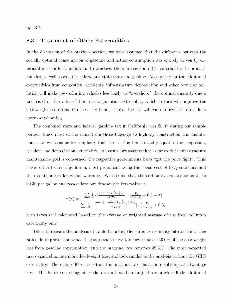
$0.30 per gallon and recalculate our deadweight loss ratios as
r(τ) =
∑i
12· |miles
yi− ˆmiles
yi (τ)
MPGi| · | Ei
MPGi+ 0.3− τ |∑
i12· |milesyi− ˆmiles
yi (
EiMPGi
+0.3)
MPGi| · ( Ei
MPGi+ 0.3)
with taxes still calculated based on the average or weighted average of the local pollution
externality only.
Table 15 repeats the analysis of Table 11 taking the carbon externality into account. The
ratios do improve somewhat. The statewide naive tax now removes 36.6% of the deadweight
loss from gasoline consumption, and the marginal tax removes 48.8%. The more targetted
taxes again eliminate more deadweight loss, and look similar to the analysis without the GHG
externality. The main difference is that the marginal tax has a more substantial advantage
here. This is not surprising, since the reason that the marginal tax provides little additional
27
benefit is because it overshoots for so many vehicles, even as it correctly taxes the dirtiest
vehicles. Table 16 shows the overshooting rates with the additional buffer of the GHG exter-
nality. The county and vintage-specific tax only overshoots about 30% of the time for both
the naive and marginal taxes.
Our assumption of an additional, untaxed externality changes the analysis for removing
the most polluting vehicles as well, shown in Table 17. Because many fewer vehicles overshoot
the optimal consumption quantity with a uniform tax, removing the most polluting vehicles
has less downside to address, and also reduces the upside of internalizing the largest external-
ities. The optimal uniform tax is actually less effective with the top 25% of the externality
distribution removed.
9 Co-benefits and the Social Cost of Carbon Pricing
The positive correlation between emissions and the sensitivity to gasoline prices has a positive
effect on the amount of local pollution benefits arising from a given GHG tax. This, in turn,
reduces the net social cost of such a policy, and to our knowledge, has been ignored in the
discussion surrounding the desirability of carbon tax or cap and trade policy.
We calculate the cost of a relatively high tax on CO2 net of the local pollution benefits.
Specifically, we use our data to simulate the change in emissions resulting from a $80 tax
on CO2, which translate to a $1 increase in the tax on gasoline.17 This is much higher than
permit prices in Europe’s cap and trade program, peaked at $40 per ton of CO2-equivalent
in 2008 and have plummeted since. It is also higher than those permit prices expected in
California’s cap and trade program trade which is expected to yield permit prices of roughly
$30 per ton of CO2-equivalent. The Waxman-Markey bill of 2009 expected a similar permit
price.
We account for both the intensive and extensive margins, as well as all the dimensions
of heterogeneity we have documented in Sections 6 and 7. For this simulation, we assume
that the tax was imposed in 1998, and use our empirical models to estimate the level of
gasoline consumption and emissions from 1998 until 2008, had gasoline prices been $1 greater.
17We assume all of the tax is passed through to consumers. Our implicit assumption is that the supplyelasticity is infinite. This is likely a fair assumption in the long-run and for policies that reduce gasolineconsumption in the near-term.
28
Appendix C provides details of the steps we take for the simulation.
Tables 18, 19, and 20 show the results of our simulation for each year from 1998-2008,
and the yearly average over the period. The first two columns shows the total reduction in
annual gasoline consumption and CO2 emissions, in millions of gallons and millions of tons,
respectively. The next two columns value the deadweight loss from the reduction in gasoline
consumption. We approximate deadweight loss as ∆P ·∆Q2
and adjust for inflation. The next
section of the table presents the social benefit resulting from the reduction in NOx, HC, and
CO due to the tax. Social benefits are valued using the marginal damages of NOx and HC
calculated by Muller and Mendelsohn (2009) and the median CO value from Matthews and
Lave (2000). Finally, the last column of the table shows the net cost of abating a ton of
carbon dioxide, accounting for the reductions in criteria pollution.
Table 18 shows the results of a simulation that does not account for heterogeneity across
emissions profiles. The reduction in gasoline consumption declines over time from around
470 million gallons in 1998 down to around 219 in 2008. The reduction in criteria pollutants
declines quickly as the fleet becomes cleaner. Nonetheless, the co-benefits of a gasoline tax
are substantial, averaging 42% of the deadweight loss over the ten year period.
Table 19 adds heterogeneity on the intensive margin, but not the extensive margins. The
total change in gasoline consumption is smaller, declining from 272 million gallons in 1998
to 107 million gallons in 2008. This is a result of more fuel efficient vehicles having a higher
average VMT. However, the reductions in criteria pollutants are much larger. In 1998 the
co-benefits are over 125% of the deadweight loss, and the net cost of abating a ton of carbon
is negative until 2001. On average, we estimate that on average benefits of a decrease in local
air pollution from a gasoline tax would be about 80% of the change in surplus between 1998
and 2008.
Finally, Table 20 adds heterogeneity on the extensive margins of scrappage and new car
purchases. The net effect of the extensive margin is a small increase in criteria pollutants,
due to the decreased scrappage vehicles 10-15 years old, and a small increase in greenhouse
gasoline abatement. The annual reduction in gasoline consumption increases from 272 million
gallons in 1998 to 110 million gallons in 2008. The amount and value of the co-benefits is
increased compared to the figures in Table 19, but the difference is relatively small. Now over
85% of the deadweight loss is compensated for by the co-benefits. The net cost of the tax is
29
negative until 2002.
Consistent with the way smog is formed, the majority the benefits come from reductions
in hydrocarbons. As discussed in the next section, most counties in California are “NOx-
constrained”. In simplest terms this means that local changes in NOx emissions do not
reduce smog, but changes in hydrocarbons do. In addition to the precursors to smog, we also
find large co-benefits arising from CO reductions.
We argue that these results should be viewed as strict lower bounds of the co-benefits
for a variety of reasons. First, we have valued the cobenefits from NOx and HCs using
the most conservative marginal damages from Muller and Mendelsohn (2009). Muller and
Mendelsohn’s estimates depend heavily on the value place upon mortality. Their baseline,
used here in Tables 18 to 20, assumes a VSL of $2 million, weighted by remaining years of
life, and they acknowledge this may not be the correct value. They also calculate a scenario
with mortality valued as in the USEPA model, with a VSL of $6 million, constant over ages.
Tables 21 and 22 repeat the simulation without and with heterogeneity from Tables 22 and
20, but value cobenefits as per Muller and Mendelsohn’s USEPA scenario. Now even without
heterogeneity the average cobenefits are greater than the deadweight loss, but decline to just
over 78% by 2008. With heterogeneity, the cobenefits average more than three times the
deadweight loss over the period, and remain twice as large in 2008.
There are other reasons why our estimates should be considered a lower bound. First, we
have ignored all other negative externalities associated with vehicles; many of these, such as
particulate matter, accidents, and congestion externalities, will be strongly correlated with
either VMT and the emissions of NOx, HCs, and CO. Second, because of the rules of the
Smog Check program many vehicles that emission standards are not required to be tested,
leading to their omission in this analysis. Third, a variety of behaviors associated with
smog check programs would lead the on-road emissions of vehicles to likely be higher than
the tested levels. These include, but are not limited to, fraud, tampering with emission-
control technologies between tests, failure to repair emission-control technologies until a test
is required, etc.
When we account for the heterogeneity in the responses to changes in gasoline prices, we
see that the co-benefits from reduced air pollution would substantially ameliorate the costs
of an increased gasoline tax. The co-benefits would have been especially substantial in the
30
late 1990s, but persist in more recent years as well, even though the fleet has become cleaner.
To put these numbers into context, Greenstone, Kopits, and Wolverton (2011) estimate the
social cost of carbon for a variety of assumptions about the discount rate, relationship between
emissions and temperatures, and models of economic activity. For 2010, using a 3 percent
discount rate, they find an average SCC of $21.40, with a 95th percentile of $64.90. Using
a 2.5 percent discount rate, the average SCC is $35.10. Our results suggest that once the
co-benefits are accounted for, a $1.00 gasoline tax (i.e., a tax of $80 per ton of CO2) would
be nearly cost-effective even at the lower of these three numbers and well below the average
social cost of capital using a 2.5 percent interest rate.18
The co-benefits vary considerably across counties. This variation comes from variation
in the marginal damages, variation in the elasticities, and variation in the heterogeneity
across vehicle types. Figure 9 illustrates the first two types of variation. Panels (a) and
(b) map the variation in the marginal damages for NOx and HC calculated by Muller and
Mendelsohn (2009). While marginal damages for HC are positively correlated with population
(correlation coefficient of 0.84), the marginal damage for NOx are negatively correlated with
both HC (0.49) and population (0.36). The reason for this has to do with the chemistry
of ground-level ozone formation. Ground-level ozone, or smog, is formed in the presence of
NOx, HCs, heat, and sunlight. When the ratio of NOx to HCs is not too large or small,
the production function of smog, in the presence of sunlight and heat, is similar to that of
a Leontiff production function. Therefore, a county can be in a region of the level-set where
increasing NOx does not increase smog production because there are not enough HCs to mix
with the additional NOx. This is known as NOx constrained. In contrast, a county may
have so much HCs such that increasing HC does not lead to more smog. This is known as
HC, or VOC, constrained.19 Therefore, the marginal damages of NOx and HC are negatively
correlated.20 Given that vehicles emit roughly equal amounts of NOx and HCs, in some
respects the average (or total) of marginal damages across NOx and HCs is more telling.
Panel (c) maps the absolute value of the elasticity of VMT across counties, calculated
18Of course, a tax somewhere below this would likely maximize welfare.19The chemistry is more complicated than this. In fact, the isoquants of the production process are backward
bending in the sense that if there is so much NOx, more NOx actually reduces smog (NO combines with O3
(ozone) to form NO2 and O2). This is known as titration.20For California the correlation is -0.36.
31
by estimating equation 25 and allowing the elasticity to vary by county of Smog Check.
The absolute value of demand elasticities tend to be positively correlated with population,
although the correlation coefficient is only 0.20.
This variation leads to the variation in the co-benefits in panel (d) of Figure 9. The
distribution is slightly skewed with a non-population weighted mean of $52.92 per ton of CO2
and median of $37.79; the standard deviation is $63.97. More populated areas have greater
co-benefits, on average. Figure 10 shows a scatterplot of the co-benefits across counties versus
the log of the counties population.21 Los Angeles is clearly an outlier with benefits of $367.28
per ton of CO2 over our sample, although as noted the median is nearly $38 with 75 percent
of counties exceeding average co-benefits of over $15.
10 Conclusions
In this paper we show three general empirical results. First, the sensitivity to a given vehicle’s
miles traveled to gasoline prices is correlated with the vehicle’s emissions. Dirtier vehicles are
more price responsive. This increases the size of the optimal uniform gasoline tax by as much
as 50 percent.
Second, gasoline taxes are an inefficient policy tool to reduce vehicle emissions. Gasoline
taxes are often promoted as a means of reducing vehicle emissions. The optimal policy would
differentially tax vehicles based on their emissions, not gasoline consumption. While gasoline
consumption and emissions are positively correlated, we show that gasoline taxes are a poor
substitute for vehicle-specific Pigouvian taxes. The deadweight loss that remains under the
optimal gasoline tax exceeds 75 percent in the second half of our sample, and is above 70
percent across all years.
Finally, the correlation we document leads to a positive result. We show that this cor-
relation significantly increases the health benefits associated with gasoline taxes. This final
results increases the attractiveness of carbon taxes as a means of reducing greenhouse gas
emissions especially when viewed in light of the fact that existing policies used to reduce
greenhouse gasoline emissions from transportation—CAFE standards, ethanol subsidies, and
the RFS—fail to take advantage of these co-benefits, and can even increase criteria pollutant
21County names are listed for a random 50 percent of the counties, plus Los Angeles.
32

emissions, because they reduce the marginal cost of an extra mile traveled. Given that previ-
ous work that has analyzed the relative efficiency of these policies to gasoline or carbon taxes
has ignored the heterogeneity that we document, such policies are less efficient than previous
thought.
33
References
Busse, Meghan, Christopher R. Knittel, and Florian Zettelmeyer. 2009. “Pain at the Pump:
The Differential Effect of Gasoline Prices on New and Used Automobile Markets.” Tech.
rep., National Bureau of Economic Research, Cambridge, MA.
Diamond, Peter A. 1973. “Consumption Externalities and Imperfect Corrective Pricing.”
The Bell Journal of Economics and Management Science 4 (2):pp. 526–538. URL http:
//www.jstor.org/stable/3003052.
Glazer, Amihai, Daniel B. Klein, and Charles Lave. 1995. “Clean on Paper, Dirty on the
Road: Troubles with California’s Smog Check.” Journal of Transport Economics and Policy
29 (1):85–92.
Greenstone, Michael, Elizabeth Kopits, and Ann Wolverton. 2011. “Estimating the Social
Cost of Carbon for Use in U.S. Federal Rulemakings: A Summary and Interpretation.”
Working Paper 16913, National Bureau of Economic Research.
Hughes, Jonathan E., Christopher R. Knittel, and Daniel Sperling. 2008. “Evidence of a Shift
in the Short-Run Price Elasticity of Gasoline Demand.” Energy Journal 29 (1).
Kahn, Matthew E. 1996. “New Evidence on Trends in Vehicle Emissions.” The RAND Journal
of Economics 27 (1):183–196.
Matthews, H. Scott and Lester B. Lave. 2000. “Applications of Environmental Valuation for
Determining Externality Costs.” Environmental Science & Technology 34 (8):1390–1395.
Morrow, Silvia and Kathy Runkle. 2005. “April 2004 Evaluation of the California Enhanced
Vehicle Inspection and Maintenance (Smog Check) Program.” Report to the legislature,
Air Resources Board.
Muller, Nicholas Z. and Robert Mendelsohn. 2009. “Efficient Pollution Regulation: Getting
the Prices Right.” American Economic Review 99 (5):1714–39.
Parry, Ian W. H. and Kenneth A. Small. 2005. “Does Britain or the United States Have the
Right Gasoline Tax?” American Economic Review 95 (4):1276–1289.
34
Sandler, Ryan. Forthcoming. “Clunkers or Junkers? Adverse Selection in a Vehicle Retirement
Program.” American Economics Journal: Economic Policy .
West, Sarah E. 2005. “Equity Implications of Vehicle Emissions Taxes.” Journal of Transport
Economics and Policy 39 (1):pp. 1–24. URL http://www.jstor.org/stable/20053948.
Westberg, Karl, Norman Cohen, and K. W. Wilson. 1971. “Carbon Monoxide: Its Role in
Photochemical Smog Formation.” Science 171 (3975):1013–1015.
35
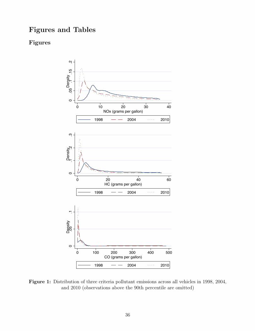
Figures and Tables
Figures
0.0
5.1
.15
.2De
nsity
0 10 20 30 40NOx (grams per gallon)
1998 2004 2010
0.1
.2.3
Dens
ity
0 20 40 60HC (grams per gallon)
1998 2004 2010
0.0
5.1
Dens
ity
0 100 200 300 400 500CO (grams per gallon)
1998 2004 2010
Figure 1: Distribution of three criteria pollutant emissions across all vehicles in 1998, 2004,and 2010 (observations above the 90th percentile are omitted)
36
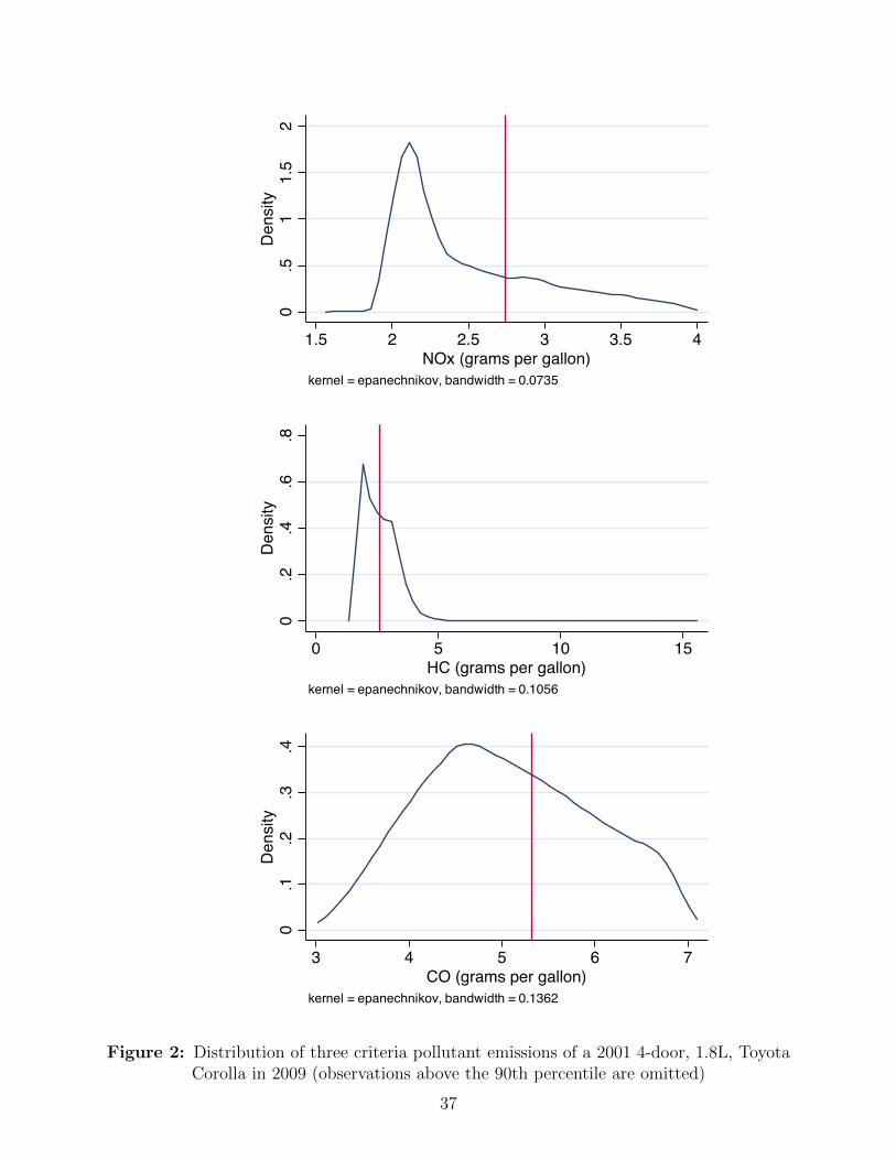
0.5
11.
52
Dens
ity
1.5 2 2.5 3 3.5 4NOx (grams per gallon)
kernel = epanechnikov, bandwidth = 0.0735
0.2
.4.6
.8De
nsity
0 5 10 15HC (grams per gallon)
kernel = epanechnikov, bandwidth = 0.1056
0.1
.2.3
.4De
nsity
3 4 5 6 7CO (grams per gallon)
kernel = epanechnikov, bandwidth = 0.1362
Figure 2: Distribution of three criteria pollutant emissions of a 2001 4-door, 1.8L, ToyotaCorolla in 2009 (observations above the 90th percentile are omitted)
37
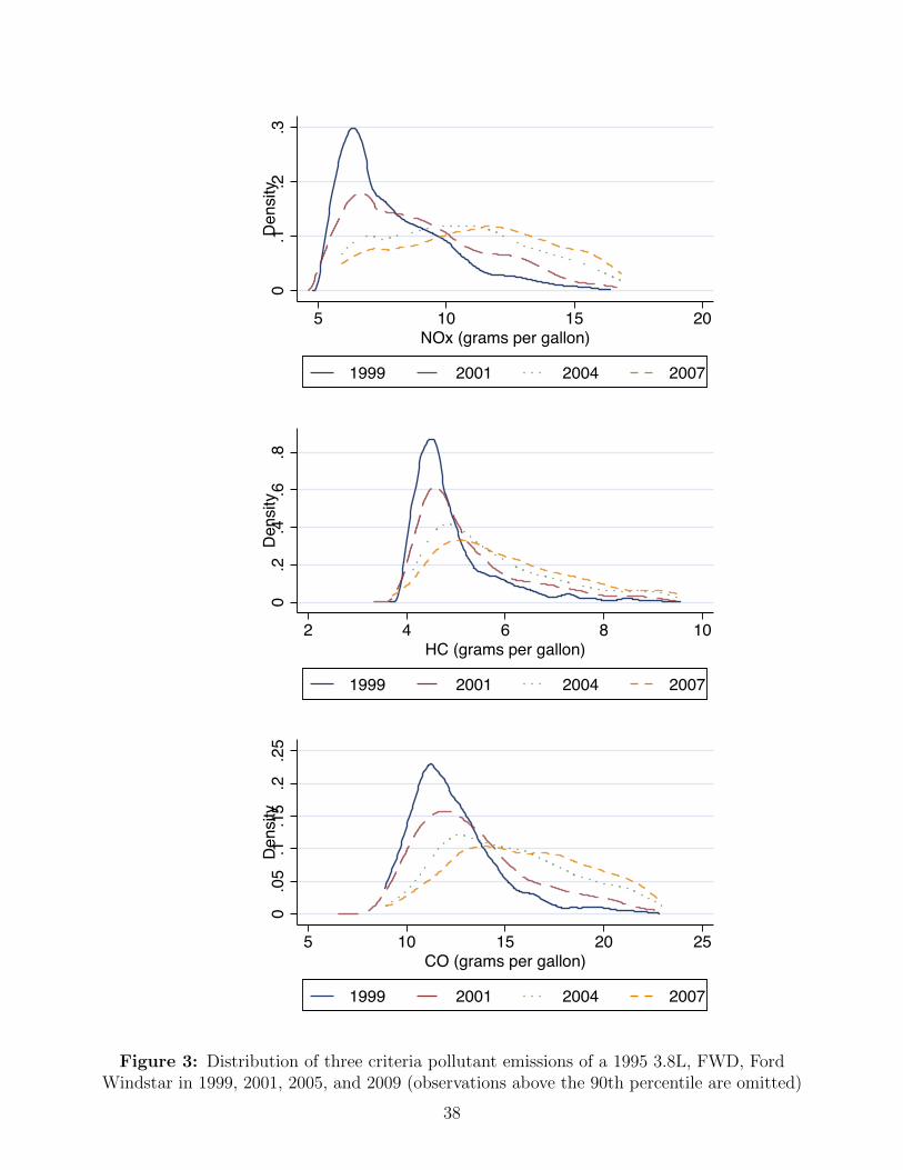
0.1
.2.3
Dens
ity
5 10 15 20NOx (grams per gallon)
1999 2001 2004 2007
0.2
.4.6
.8De
nsity
2 4 6 8 10HC (grams per gallon)
1999 2001 2004 2007
0.0
5.1
.15
.2.2
5De
nsity
5 10 15 20 25CO (grams per gallon)
1999 2001 2004 2007
Figure 3: Distribution of three criteria pollutant emissions of a 1995 3.8L, FWD, FordWindstar in 1999, 2001, 2005, and 2009 (observations above the 90th percentile are omitted)
38
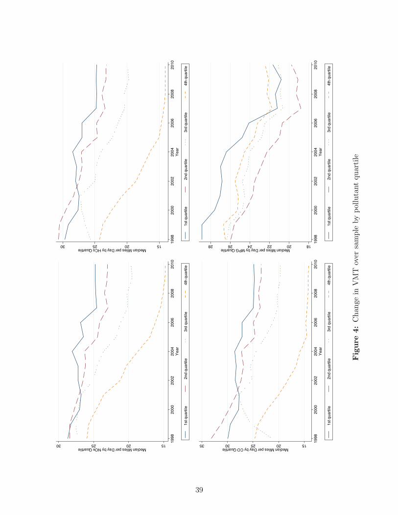
15202530Median Miles per Day by NOx Quartile
1998
2000
2002
2004
2006
2008
2010
Year
1st q
uarti
le2n
d qu
artil
e3r
d qu
artil
e4t
h qu
artil
e
15202530Median Miles per Day by HCs Quartile
1998
2000
2002
2004
2006
2008
2010
Year
1st q
uarti
le2n
d qu
artil
e3r
d qu
artil
e4t
h qu
artil
e
1520253035Median Miles per Day by CO Quartile
1998
2000
2002
2004
2006
2008
2010
Year
1st q
uarti
le2n
d qu
artil
e3r
d qu
artil
e4t
h qu
artil
e
182022242628Median Miles per Day by MPG Quartile
1998
2000
2002
2004
2006
2008
2010
Year
1st q
uarti
le2n
d qu
artil
e3r
d qu
artil
e4t
h qu
artil
e
Fig
ure
4:
Chan
gein
VM
Tov
ersa
mple
by
pol
luta
nt
quar
tile
39
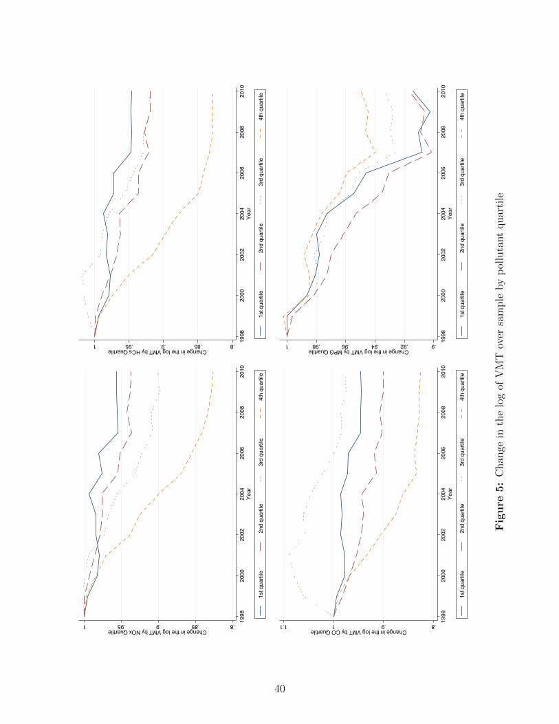
.8.85.9.951Change in the log VMT by NOx Quartile
1998
2000
2002
2004
2006
2008
2010
Year
1st q
uarti
le2n
d qu
artil
e3r
d qu
artil
e4t
h qu
artil
e
.8.85.9.951Change in the log VMT by HCs Quartile
1998
2000
2002
2004
2006
2008
2010
Year
1st q
uarti
le2n
d qu
artil
e3r
d qu
artil
e4t
h qu
artil
e
.8.911.1Change in the log VMT by CO Quartile
1998
2000
2002
2004
2006
2008
2010
Year
1st q
uarti
le2n
d qu
artil
e3r
d qu
artil
e4t
h qu
artil
e
.9.92.94.96.981Change in the log VMT by MPG Quartile
1998
2000
2002
2004
2006
2008
2010
Year
1st q
uarti
le2n
d qu
artil
e3r
d qu
artil
e4t
h qu
artil
e
Fig
ure
5:
Chan
gein
the
log
ofV
MT
over
sam
ple
by
pol
luta
nt
quar
tile
40
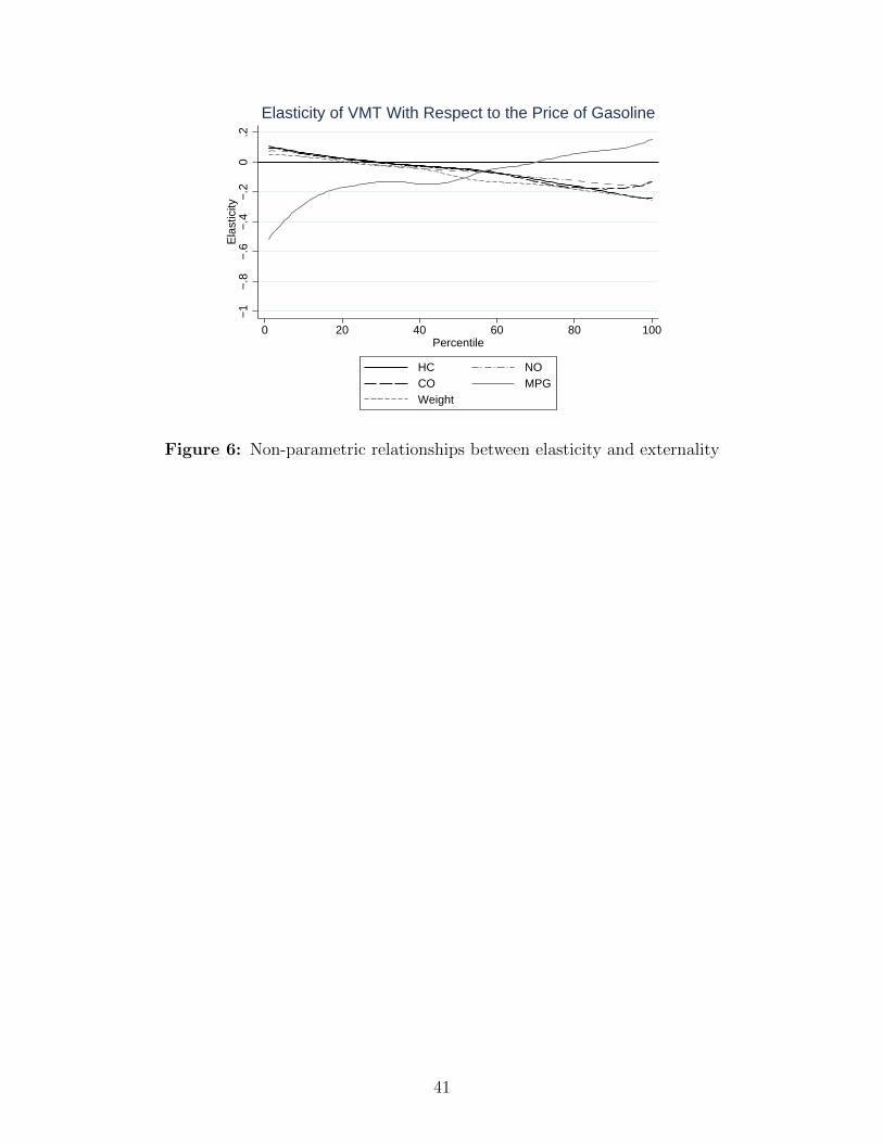
−1
−.8
−.6
−.4
−.2
0.2
Ela
stic
ity
0 20 40 60 80 100Percentile
HC NO CO MPG Weight
Elasticity of VMT With Respect to the Price of Gasoline
Figure 6: Non-parametric relationships between elasticity and externality
41
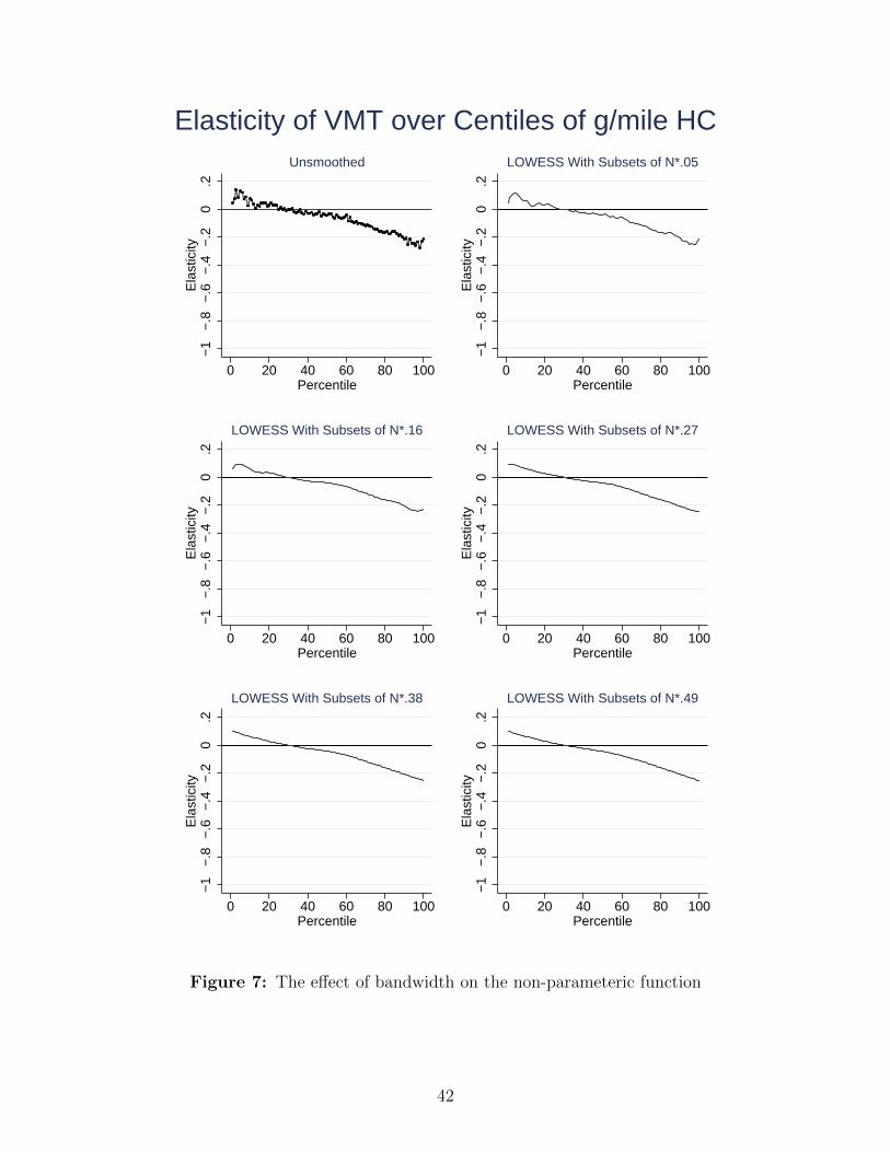
−1
−.8
−.6
−.4
−.2
0.2
Ela
stic
ity
0 20 40 60 80 100Percentile
Unsmoothed
−1
−.8
−.6
−.4
−.2
0.2
Ela
stic
ity
0 20 40 60 80 100Percentile
LOWESS With Subsets of N*.05
−1
−.8
−.6
−.4
−.2
0.2
Ela
stic
ity
0 20 40 60 80 100Percentile
LOWESS With Subsets of N*.16
−1
−.8
−.6
−.4
−.2
0.2
Ela
stic
ity
0 20 40 60 80 100Percentile
LOWESS With Subsets of N*.27
−1
−.8
−.6
−.4
−.2
0.2
Ela
stic
ity
0 20 40 60 80 100Percentile
LOWESS With Subsets of N*.38
−1
−.8
−.6
−.4
−.2
0.2
Ela
stic
ity
0 20 40 60 80 100Percentile
LOWESS With Subsets of N*.49
Elasticity of VMT over Centiles of g/mile HC
Figure 7: The effect of bandwidth on the non-parameteric function
42
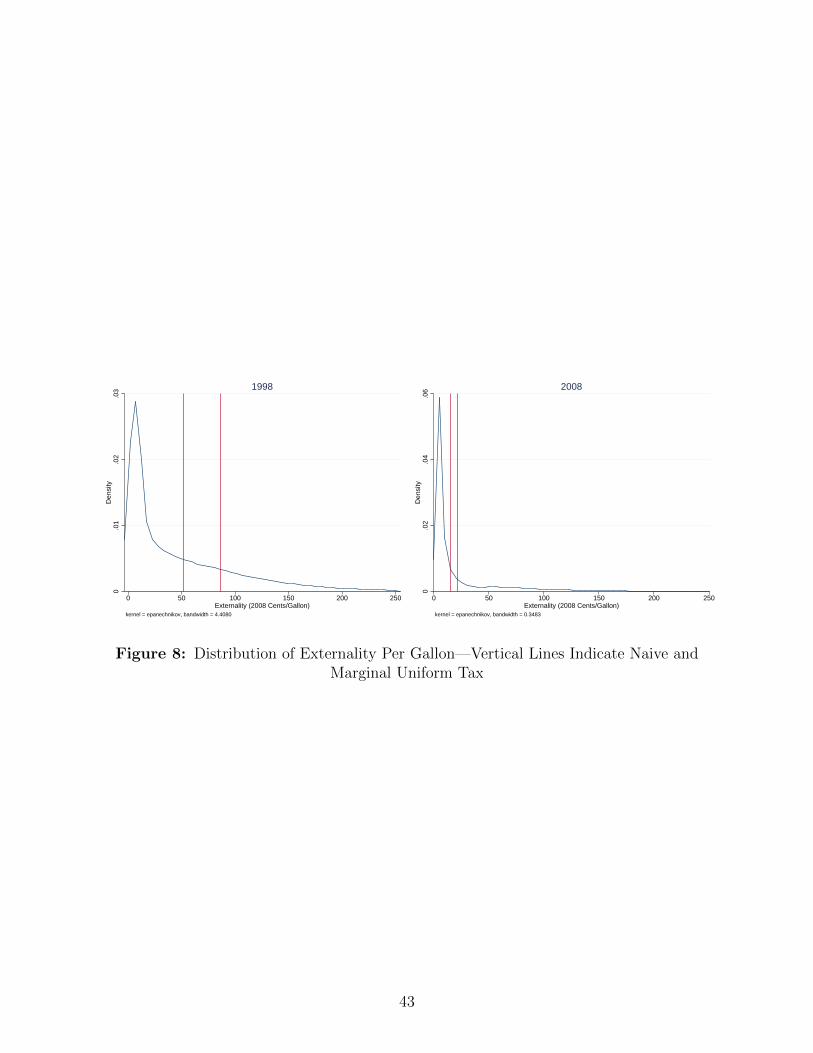
0.0
1.0
2.0
3D
ensi
ty
0 50 100 150 200 250Externality (2008 Cents/Gallon)
kernel = epanechnikov, bandwidth = 4.4080
1998
0.0
2.0
4.0
6D
ensi
ty
0 50 100 150 200 250Externality (2008 Cents/Gallon)
kernel = epanechnikov, bandwidth = 0.3483
2008
Figure 8: Distribution of Externality Per Gallon—Vertical Lines Indicate Naive andMarginal Uniform Tax
43
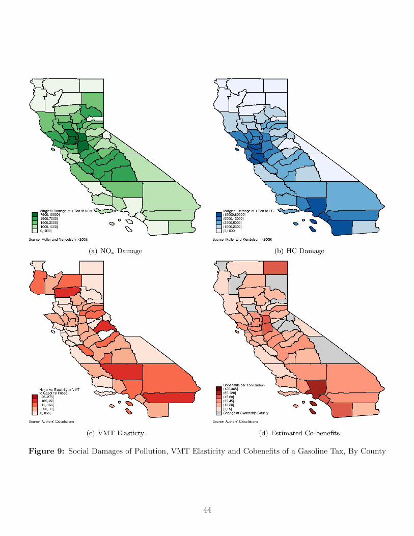
Figure 9: Social Damages of Pollution, VMT Elasticity and Cobenefits of a Gasoline Tax, By County
44
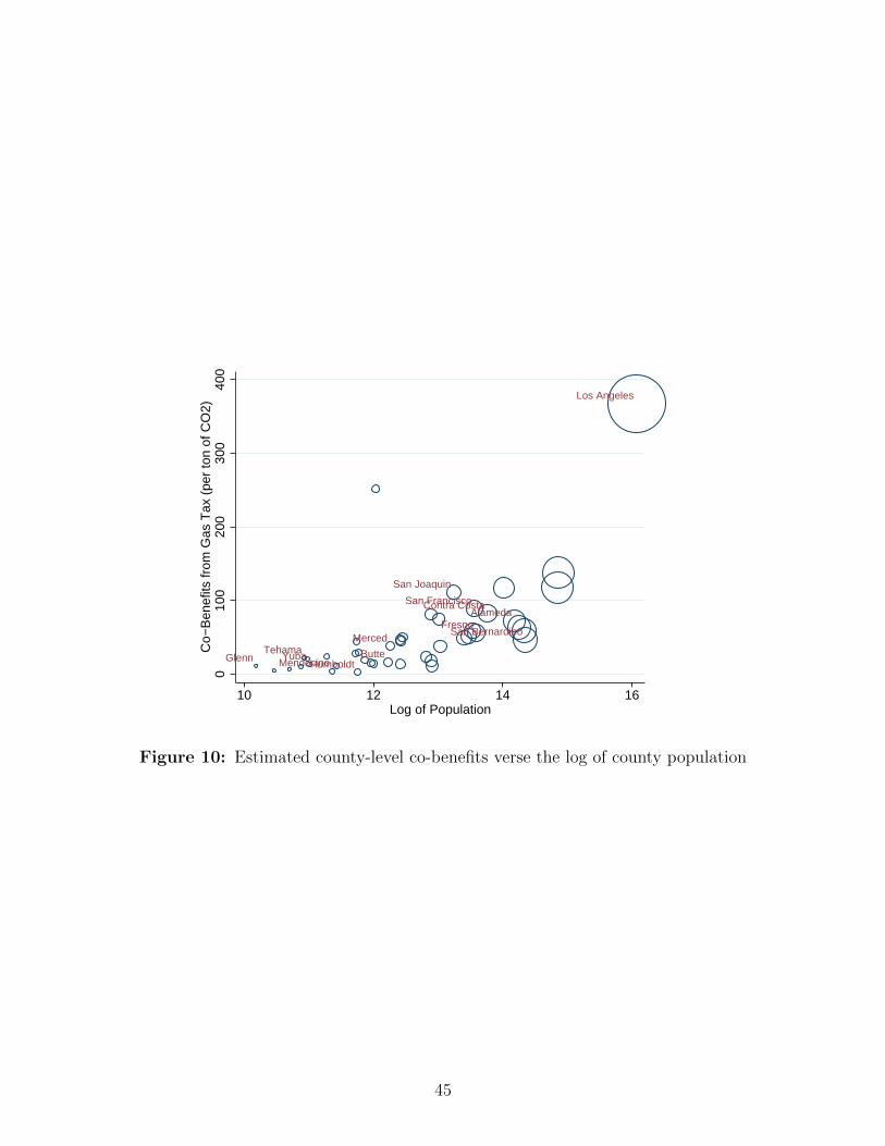
Alameda
Butte
Contra Costa
Fresno
GlennHumboldt
Los Angeles
Mendocino
MercedSan Bernardino
San Francisco
San Joaquin
TehamaYuba
010
020
030
040
0C
o−B
enef
its fr
om G
as T
ax (
per
ton
of C
O2)
10 12 14 16Log of Population
Figure 10: Estimated county-level co-benefits verse the log of county population
45
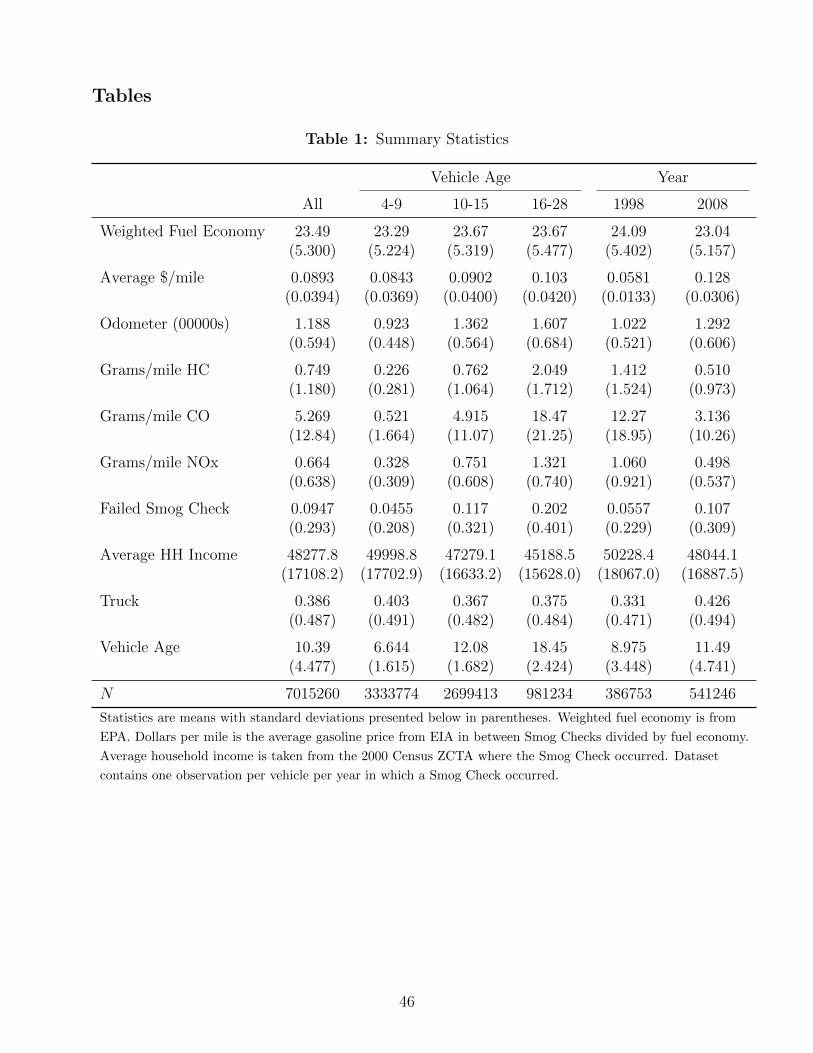
Tables
Table 1: Summary Statistics
Vehicle Age Year
All 4-9 10-15 16-28 1998 2008
Weighted Fuel Economy 23.49 23.29 23.67 23.67 24.09 23.04(5.300) (5.224) (5.319) (5.477) (5.402) (5.157)
Average $/mile 0.0893 0.0843 0.0902 0.103 0.0581 0.128(0.0394) (0.0369) (0.0400) (0.0420) (0.0133) (0.0306)
Odometer (00000s) 1.188 0.923 1.362 1.607 1.022 1.292(0.594) (0.448) (0.564) (0.684) (0.521) (0.606)
Grams/mile HC 0.749 0.226 0.762 2.049 1.412 0.510(1.180) (0.281) (1.064) (1.712) (1.524) (0.973)
Grams/mile CO 5.269 0.521 4.915 18.47 12.27 3.136(12.84) (1.664) (11.07) (21.25) (18.95) (10.26)
Grams/mile NOx 0.664 0.328 0.751 1.321 1.060 0.498(0.638) (0.309) (0.608) (0.740) (0.921) (0.537)
Failed Smog Check 0.0947 0.0455 0.117 0.202 0.0557 0.107(0.293) (0.208) (0.321) (0.401) (0.229) (0.309)
Average HH Income 48277.8 49998.8 47279.1 45188.5 50228.4 48044.1(17108.2) (17702.9) (16633.2) (15628.0) (18067.0) (16887.5)
Truck 0.386 0.403 0.367 0.375 0.331 0.426(0.487) (0.491) (0.482) (0.484) (0.471) (0.494)
Vehicle Age 10.39 6.644 12.08 18.45 8.975 11.49(4.477) (1.615) (1.682) (2.424) (3.448) (4.741)
N 7015260 3333774 2699413 981234 386753 541246
Statistics are means with standard deviations presented below in parentheses. Weighted fuel economy is from
EPA. Dollars per mile is the average gasoline price from EIA in between Smog Checks divided by fuel economy.
Average household income is taken from the 2000 Census ZCTA where the Smog Check occurred. Dataset
contains one observation per vehicle per year in which a Smog Check occurred.
46
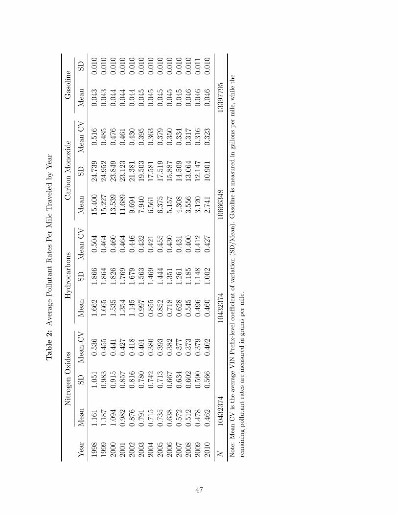
Table
2:
Ave
rage
Pol
luta
nt
Rat
esP
erM
ile
Tra
vele
dby
Yea
r
Nit
roge
nO
xid
esH
ydro
carb
ons
Car
bon
Mon
oxid
eG
asol
ine
Yea
rM
ean
SD
Mea
nC
VM
ean
SD
Mea
nC
VM
ean
SD
Mea
nC
VM
ean
SD
1998
1.16
11.
051
0.53
61.
662
1.86
60.
504
15.4
0024
.739
0.51
60.
043
0.01
019
991.
187
0.98
30.
455
1.66
51.
864
0.46
415
.227
24.9
520.
485
0.04
30.
010
2000
1.09
40.
915
0.44
11.
535
1.82
60.
460
13.5
3923
.849
0.47
60.
044
0.01
020
010.
982
0.85
70.
427
1.35
41.
769
0.46
411
.689
23.1
230.
461
0.04
40.
010
2002
0.87
60.
816
0.41
81.
145
1.67
90.
446
9.69
421
.381
0.43
00.
044
0.01
020
030.
791
0.78
00.
401
0.99
71.
563
0.43
27.
940
19.5
030.
395
0.04
50.
010
2004
0.71
50.
742
0.38
00.
855
1.46
90.
421
6.56
117
.581
0.36
30.
045
0.01
020
050.
735
0.71
30.
393
0.85
21.
444
0.45
56.
375
17.5
190.
379
0.04
50.
010
2006
0.63
80.
667
0.38
20.
718
1.35
10.
430
5.15
715
.887
0.35
00.
045
0.01
020
070.
572
0.63
40.
377
0.62
81.
261
0.43
14.
308
14.5
090.
334
0.04
50.
010
2008
0.51
20.
602
0.37
30.
545
1.18
50.
400
3.55
613
.064
0.31
70.
046
0.01
020
090.
478
0.59
00.
379
0.49
61.
148
0.41
23.
120
12.1
470.
316
0.04
60.
011
2010
0.46
20.
566
0.40
20.
460
1.00
20.
427
2.74
110
.901
0.32
30.
046
0.01
0
N10
4323
7410
4323
7410
6663
4813
3977
95
Not
e:M
ean
CV
isth
eav
erag
eV
INP
refi
x-l
evel
coeffi
cien
tof
vari
ati
on
(SD
/M
ean
).G
aso
lin
eis
mea
sure
din
gall
on
sp
erm
ile,
whil
eth
e
rem
ain
ing
pol
luta
nt
rate
sar
em
easu
red
ingra
ms
per
mil
e.
47

Table 3: Vehicle Miles Traveled, Dollars Per Mile, and Nitrogen Oxides (Quartiles by year)
(1) (2) (3) (4) (5) (6) (7)Model 1 Model 2 Model 3 Model 4 Model 5 Model 6 Model 7
ln(DPM) -0.265** -0.117** -0.177** -0.147** -0.044(0.045) (0.038) (0.027) (0.025) (0.032)
ln(DPM) * NO Q1 -0.037** 0.041+(0.011) (0.023)
ln(DPM) * NO Q2 -0.086** -0.062*(0.011) (0.026)
ln(DPM) * NO Q3 -0.133** -0.158**(0.011) (0.027)
ln(DPM) * NO Q4 -0.189** -0.288**(0.012) (0.030)
ln(DPM)*NO Centile -0.001**(0.000)
NO Q2 -0.083** 0.378(0.012) (0.800)
NO Q3 -0.144** -1.246(0.016) (1.012)
NO Q4 -0.166** -2.297*(0.020) (1.116)
NO Centile -0.001(0.001)
Truck 0.058+ 0.062 0.049** 0.006(0.035) (0.046) (0.009) (0.057)
Time Trend -0.281** -0.355** -0.388** -0.318** -0.019 -0.027 -0.046(0.040) (0.029) (0.026) (0.023) (0.041) (0.070) (0.053)
Time Trend-Squared 0.002** 0.003** 0.003** 0.002** 0.000 -0.000 0.000(0.000) (0.000) (0.000) (0.000) (0.000) (0.001) (0.001)
Year Fixed Effects Yes Yes Yes Yes Yes Yes YesVintage Fixed Effects Yes Yes Yes Yes Yes Yes YesDemographics Yes Yes Yes Yes Yes Yes YesMake Fixed Effects No Yes Yes No No No NoVin Prefix Fixed Effects No No No Yes No No NoVehicle Fixed Effects No No No No Yes Yes Yes
Observations 3640433 3640433 2979289 3640433 3640433 2979289 2979289R-squared 0.216 0.224 0.234 0.149 0.120 0.116 0.117
48
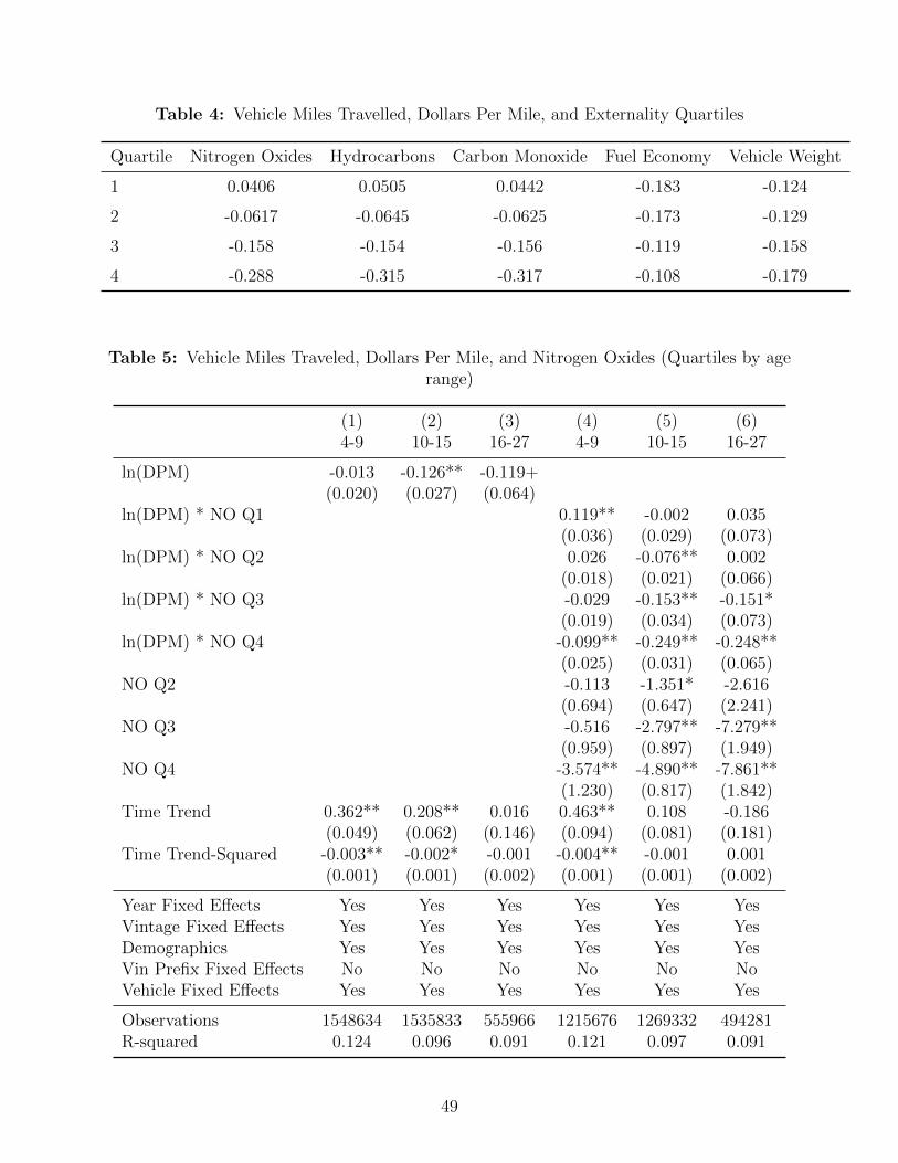
Table 4: Vehicle Miles Travelled, Dollars Per Mile, and Externality Quartiles
Quartile Nitrogen Oxides Hydrocarbons Carbon Monoxide Fuel Economy Vehicle Weight
1 0.0406 0.0505 0.0442 -0.183 -0.124
2 -0.0617 -0.0645 -0.0625 -0.173 -0.129
3 -0.158 -0.154 -0.156 -0.119 -0.158
4 -0.288 -0.315 -0.317 -0.108 -0.179
Table 5: Vehicle Miles Traveled, Dollars Per Mile, and Nitrogen Oxides (Quartiles by agerange)
(1) (2) (3) (4) (5) (6)4-9 10-15 16-27 4-9 10-15 16-27
ln(DPM) -0.013 -0.126** -0.119+(0.020) (0.027) (0.064)
ln(DPM) * NO Q1 0.119** -0.002 0.035(0.036) (0.029) (0.073)
ln(DPM) * NO Q2 0.026 -0.076** 0.002(0.018) (0.021) (0.066)
ln(DPM) * NO Q3 -0.029 -0.153** -0.151*(0.019) (0.034) (0.073)
ln(DPM) * NO Q4 -0.099** -0.249** -0.248**(0.025) (0.031) (0.065)
NO Q2 -0.113 -1.351* -2.616(0.694) (0.647) (2.241)
NO Q3 -0.516 -2.797** -7.279**(0.959) (0.897) (1.949)
NO Q4 -3.574** -4.890** -7.861**(1.230) (0.817) (1.842)
Time Trend 0.362** 0.208** 0.016 0.463** 0.108 -0.186(0.049) (0.062) (0.146) (0.094) (0.081) (0.181)
Time Trend-Squared -0.003** -0.002* -0.001 -0.004** -0.001 0.001(0.001) (0.001) (0.002) (0.001) (0.001) (0.002)
Year Fixed Effects Yes Yes Yes Yes Yes YesVintage Fixed Effects Yes Yes Yes Yes Yes YesDemographics Yes Yes Yes Yes Yes YesVin Prefix Fixed Effects No No No No No NoVehicle Fixed Effects Yes Yes Yes Yes Yes Yes
Observations 1548634 1535833 555966 1215676 1269332 494281R-squared 0.124 0.096 0.091 0.121 0.097 0.091
49
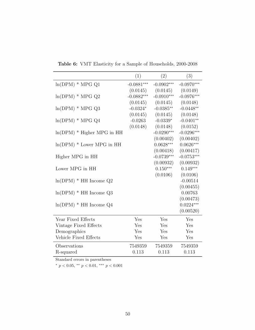
Table 6: VMT Elasticity for a Sample of Households, 2000-2008
(1) (2) (3)
ln(DPM) * MPG Q1 -0.0881∗∗∗ -0.0902∗∗∗ -0.0970∗∗∗
(0.0145) (0.0145) (0.0149)ln(DPM) * MPG Q2 -0.0882∗∗∗ -0.0910∗∗∗ -0.0976∗∗∗
(0.0145) (0.0145) (0.0148)ln(DPM) * MPG Q3 -0.0324∗ -0.0385∗∗ -0.0448∗∗
(0.0145) (0.0145) (0.0148)ln(DPM) * MPG Q4 -0.0263 -0.0339∗ -0.0401∗∗
(0.0148) (0.0148) (0.0152)ln(DPM) * Higher MPG in HH -0.0290∗∗∗ -0.0296∗∗∗
(0.00402) (0.00402)ln(DPM) * Lower MPG in HH 0.0628∗∗∗ 0.0626∗∗∗
(0.00418) (0.00417)Higher MPG in HH -0.0739∗∗∗ -0.0753∗∗∗
(0.00932) (0.00932)Lower MPG in HH 0.150∗∗∗ 0.149∗∗∗
(0.0106) (0.0106)ln(DPM) * HH Income Q2 -0.00514
(0.00455)ln(DPM) * HH Income Q3 0.00763
(0.00473)ln(DPM) * HH Income Q4 0.0224∗∗∗
(0.00520)
Year Fixed Effects Yes Yes YesVintage Fixed Effects Yes Yes YesDemographics Yes Yes YesVehicle Fixed Effects Yes Yes Yes
Observations 7549359 7549359 7549359R-squared 0.113 0.113 0.113
Standard errors in parentheses∗ p < 0.05, ∗∗ p < 0.01, ∗∗∗ p < 0.001
50
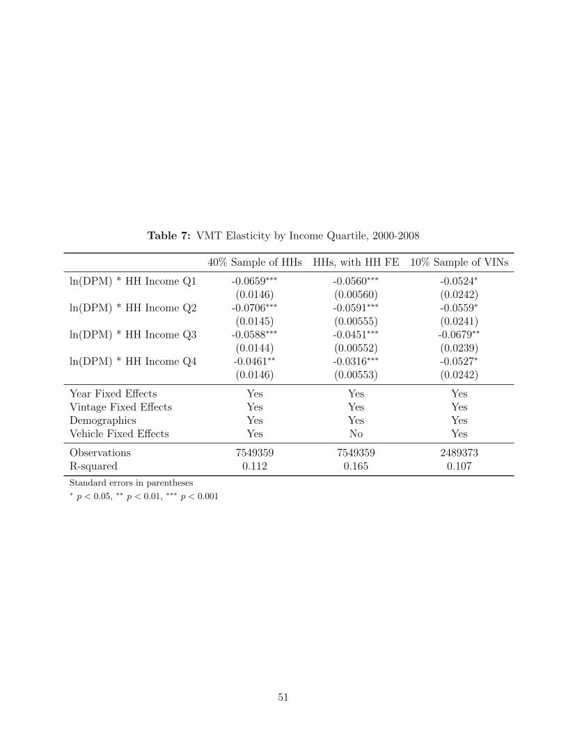
Table 7: VMT Elasticity by Income Quartile, 2000-2008
40% Sample of HHs HHs, with HH FE 10% Sample of VINs
ln(DPM) * HH Income Q1 -0.0659∗∗∗ -0.0560∗∗∗ -0.0524∗
(0.0146) (0.00560) (0.0242)ln(DPM) * HH Income Q2 -0.0706∗∗∗ -0.0591∗∗∗ -0.0559∗
(0.0145) (0.00555) (0.0241)ln(DPM) * HH Income Q3 -0.0588∗∗∗ -0.0451∗∗∗ -0.0679∗∗
(0.0144) (0.00552) (0.0239)ln(DPM) * HH Income Q4 -0.0461∗∗ -0.0316∗∗∗ -0.0527∗
(0.0146) (0.00553) (0.0242)
Year Fixed Effects Yes Yes YesVintage Fixed Effects Yes Yes YesDemographics Yes Yes YesVehicle Fixed Effects Yes No Yes
Observations 7549359 7549359 2489373R-squared 0.112 0.165 0.107
Standard errors in parentheses∗ p < 0.05, ∗∗ p < 0.01, ∗∗∗ p < 0.001
51
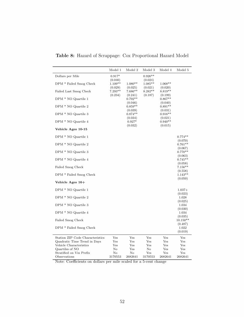
Table 8: Hazard of Scrappage: Cox Proportional Hazard Model
Model 1 Model 2 Model 3 Model 4 Model 5
Dollars per Mile 0.917* 0.926**(0.040) (0.024)
DPM * Failed Smog Check 1.109** 1.080** 1.085** 1.068**(0.029) (0.025) (0.021) (0.020)
Failed Last Smog Check 7.293** 7.686** 8.282** 8.819**(0.234) (0.241) (0.187) (0.199)
DPM * NO Quartile 1 0.792** 0.867**(0.046) (0.040)
DPM * NO Quartile 2 0.859** 0.891**(0.039) (0.031)
DPM * NO Quartile 3 0.874** 0.916**(0.034) (0.021)
DPM * NO Quartile 4 0.927* 0.940**(0.032) (0.015)
Vehicle Ages 10-15
DPM * NO Quartile 1 0.774**(0.070)
DPM * NO Quartile 2 0.761**(0.067)
DPM * NO Quartile 3 0.770**(0.063)
DPM * NO Quartile 4 0.745**(0.058)
Failed Smog Check 7.156**(0.558)
DPM * Failed Smog Check 1.143**(0.050)
Vehicle Ages 16+
DPM * NO Quartile 1 1.037+(0.023)
DPM * NO Quartile 2 1.028(0.025)
DPM * NO Quartile 3 1.034(0.030)
DPM * NO Quartile 4 1.034(0.035)
Failed Smog Check 10.150**(0.487)
DPM * Failed Smog Check 1.022(0.019)
Station ZIP Code Characteristics Yes Yes Yes Yes YesQuadratic Time Trend in Days Yes Yes Yes Yes YesVehicle Characteristics Yes Yes Yes Yes YesQuartiles of NO No Yes No Yes YesStratified on Vin Prefix No No Yes Yes YesObservations 3170553 2682641 3170553 2682641 2682641
Note: Coefficients on dollars per mile scaled for a 5-cent change
52
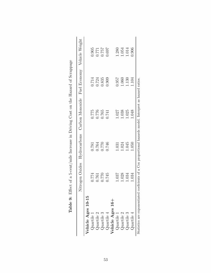
Table
9:
Eff
ect
ofa
5-ce
nt/
mile
Incr
ease
inD
rivin
gC
ost
onth
eH
azar
dof
Scr
appag
e
Nit
roge
nO
xid
esH
ydro
carb
ons
Car
bon
Mon
oxid
eF
uel
Eco
nom
yV
ehic
leW
eigh
t
Veh
icle
Ages
10-1
5Q
uar
tile
10.
774
0.78
10.
775
0.71
40.
905
Quar
tile
20.
761
0.76
40.
776
0.72
40.
771
Quar
tile
30.
770
0.77
00.
765
0.83
50.
757
Quar
tile
40.
745
0.74
60.
741
0.90
90.
697
Veh
icle
Ages
16+
Quar
tile
11.
037
1.03
11.
027
0.95
71.
280
Quar
tile
21.
028
1.02
41.
038
1.06
01.
054
Quar
tile
31.
034
1.04
51.
025
1.13
01.
014
Quar
tile
41.
034
1.05
01.
048
1.10
40.
906
Sta
tist
ics
are
exp
onen
tiat
edco
efici
ents
of
aC
oxp
rop
ort
ion
al
haza
rds
mod
el.
Inte
rpre
tas
haza
rdra
tios.
53
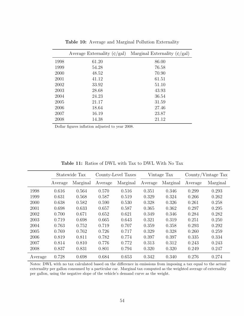
Table 10: Average and Marginal Pollution Externality
Average Externality (¢/gal) Marginal Externality (¢/gal)
1998 61.20 86.001999 54.28 76.582000 48.52 70.902001 41.12 61.512002 33.92 51.102003 28.68 43.932004 24.23 36.542005 21.17 31.592006 18.64 27.462007 16.19 23.872008 14.38 21.12
Dollar figures inflation adjusted to year 2008.
Table 11: Ratios of DWL with Tax to DWL With No Tax
Statewide Tax County-Level Taxes Vintage Tax County/Vintage Tax
Average Marginal Average Marginal Average Marginal Average Marginal
1998 0.616 0.564 0.570 0.516 0.351 0.346 0.299 0.2931999 0.631 0.568 0.587 0.519 0.329 0.324 0.266 0.2622000 0.638 0.582 0.590 0.530 0.328 0.326 0.261 0.2582001 0.698 0.633 0.657 0.587 0.365 0.362 0.297 0.2952002 0.700 0.671 0.652 0.621 0.349 0.346 0.284 0.2822003 0.719 0.698 0.665 0.643 0.321 0.319 0.251 0.2502004 0.763 0.752 0.719 0.707 0.359 0.358 0.293 0.2922005 0.769 0.762 0.726 0.717 0.329 0.328 0.260 0.2592006 0.819 0.811 0.782 0.774 0.397 0.397 0.335 0.3342007 0.814 0.810 0.776 0.772 0.313 0.312 0.243 0.2432008 0.837 0.831 0.801 0.794 0.320 0.320 0.249 0.247
Average 0.728 0.698 0.684 0.653 0.342 0.340 0.276 0.274
Notes: DWL with no tax calculated based on the difference in emissions from imposing a tax equal to the actualexternality per gallon consumed by a particular car. Marginal tax computed as the weighted average of externalityper gallon, using the negative slope of the vehicle’s demand curve as the weight.
54

Table 12: Proportion of Vehicles for which a Uniform Tax Overshoots the Optimal Tax
Mean
Fleet Average 0.724Fleet Marginal 0.794County Average 0.714County Marginal 0.784Vintage Average 0.706Vintage Marginal 0.726County/Vintage Average 0.671County/Vintage Marginal 0.706
N 3605189
mean coefficients∗ p < 0.05, ∗∗ p < 0.01, ∗∗∗ p < 0.001
Table 13: Ratios of DWL with Tax to DWL With No Tax, Scrapping Most PollutingVehicles
Percentile Scrapped
None 1% 2% 5% 10% 25%
1998 0.564 0.466 0.441 0.415 0.405 0.4151999 0.568 0.474 0.458 0.442 0.437 0.4442000 0.582 0.493 0.478 0.462 0.459 0.4602001 0.633 0.528 0.511 0.495 0.491 0.4372002 0.671 0.585 0.573 0.560 0.556 0.4962003 0.698 0.629 0.619 0.608 0.604 0.4722004 0.752 0.675 0.666 0.654 0.645 0.4392005 0.762 0.699 0.689 0.672 0.648 0.3712006 0.811 0.731 0.720 0.700 0.658 0.3442007 0.810 0.759 0.748 0.725 0.658 0.3552008 0.831 0.780 0.768 0.737 0.612 0.349
Average 0.698 0.620 0.606 0.588 0.561 0.417
Notes: DWL with no tax calculated based on the difference inemissions from imposing a tax equal to the actual externalityper gallon consumed by a particular car. Marginal tax com-puted as the weighted average of externality per gallon, usingthe negative slope of the vehicle’s demand curve as the weight.
55
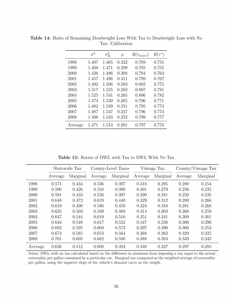
Table 14: Ratio of Remaining Deadweight Loss With Tax to Deadweight Loss with NoTax: Calibration
σ2 σ2B ρ R(τnaive) R(τ ∗)
1998 1.407 1.465 0.322 0.789 0.7551999 1.408 1.471 0.299 0.785 0.7552000 1.438 1.486 0.308 0.794 0.7632001 1.457 1.496 0.311 0.799 0.7672002 1.492 1.506 0.283 0.802 0.7752003 1.517 1.535 0.283 0.807 0.7812004 1.525 1.531 0.265 0.806 0.7822005 1.474 1.539 0.265 0.796 0.7712006 1.482 1.539 0.251 0.795 0.7732007 1.487 1.547 0.247 0.796 0.7742008 1.498 1.533 0.252 0.799 0.777
Average 1.471 1.513 0.281 0.797 0.770
Table 15: Ratios of DWL with Tax to DWL With No Tax
Statewide Tax County-Level Taxes Vintage Tax County/Vintage Tax
Average Marginal Average Marginal Average Marginal Average Marginal
1998 0.571 0.434 0.536 0.397 0.318 0.295 0.280 0.2541999 0.590 0.426 0.558 0.390 0.301 0.279 0.256 0.2352000 0.591 0.433 0.556 0.397 0.299 0.281 0.250 0.2352001 0.648 0.472 0.619 0.440 0.329 0.312 0.280 0.2662002 0.619 0.490 0.586 0.459 0.324 0.310 0.281 0.2682003 0.625 0.503 0.589 0.469 0.314 0.303 0.268 0.2592004 0.647 0.544 0.619 0.516 0.351 0.341 0.309 0.3012005 0.644 0.548 0.617 0.522 0.347 0.336 0.306 0.2962006 0.692 0.595 0.669 0.573 0.397 0.390 0.360 0.3532007 0.674 0.585 0.653 0.564 0.368 0.362 0.329 0.3252008 0.701 0.605 0.682 0.586 0.388 0.383 0.349 0.345
Average 0.636 0.512 0.608 0.483 0.340 0.327 0.297 0.285
Notes: DWL with no tax calculated based on the difference in emissions from imposing a tax equal to the actualexternality per gallon consumed by a particular car. Marginal tax computed as the weighted average of externalityper gallon, using the negative slope of the vehicle’s demand curve as the weight.
56
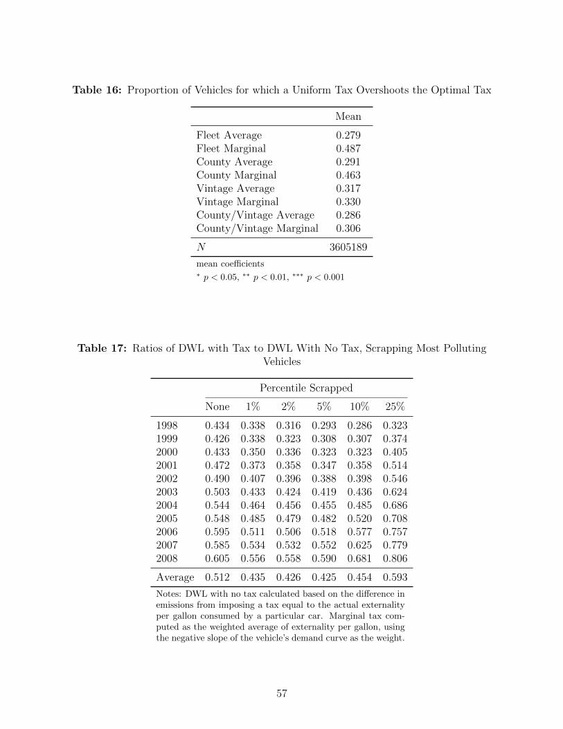
Table 16: Proportion of Vehicles for which a Uniform Tax Overshoots the Optimal Tax
Mean
Fleet Average 0.279Fleet Marginal 0.487County Average 0.291County Marginal 0.463Vintage Average 0.317Vintage Marginal 0.330County/Vintage Average 0.286County/Vintage Marginal 0.306
N 3605189
mean coefficients∗ p < 0.05, ∗∗ p < 0.01, ∗∗∗ p < 0.001
Table 17: Ratios of DWL with Tax to DWL With No Tax, Scrapping Most PollutingVehicles
Percentile Scrapped
None 1% 2% 5% 10% 25%
1998 0.434 0.338 0.316 0.293 0.286 0.3231999 0.426 0.338 0.323 0.308 0.307 0.3742000 0.433 0.350 0.336 0.323 0.323 0.4052001 0.472 0.373 0.358 0.347 0.358 0.5142002 0.490 0.407 0.396 0.388 0.398 0.5462003 0.503 0.433 0.424 0.419 0.436 0.6242004 0.544 0.464 0.456 0.455 0.485 0.6862005 0.548 0.485 0.479 0.482 0.520 0.7082006 0.595 0.511 0.506 0.518 0.577 0.7572007 0.585 0.534 0.532 0.552 0.625 0.7792008 0.605 0.556 0.558 0.590 0.681 0.806
Average 0.512 0.435 0.426 0.425 0.454 0.593
Notes: DWL with no tax calculated based on the difference inemissions from imposing a tax equal to the actual externalityper gallon consumed by a particular car. Marginal tax com-puted as the weighted average of externality per gallon, usingthe negative slope of the vehicle’s demand curve as the weight.
57
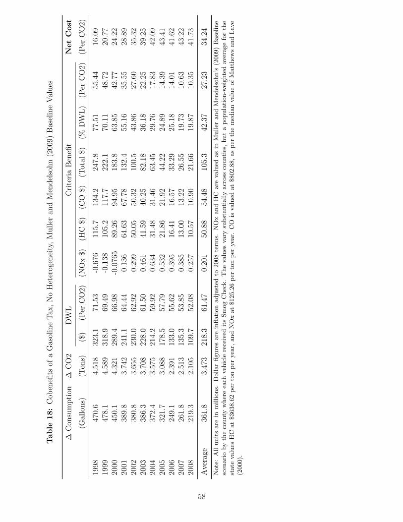
Table
18:
Cob
enefi
tsof
aG
asol
ine
Tax
,N
oH
eter
ogen
eity
,M
uller
and
Men
del
sohn
(200
9)B
asel
ine
Val
ues
∆C
onsu
mpti
on∆
CO
2D
WL
Cri
teri
aB
enefi
tN
et
Cost
(Gal
lons)
(Ton
s)($
)(P
erC
O2)
(NO
x$)
(HC
$)(C
O$)
(Tot
al$)
(%D
WL
)(P
erC
O2)
(Per
CO
2)
1998
470.
64.
518
323.
171
.53
-0.6
7611
5.7
134.
224
7.8
77.5
155
.44
16.0
919
9947
8.1
4.58
931
8.9
69.4
9-0
.138
105.
211
7.7
222.
170
.11
48.7
220
.77
2000
450.
14.
321
289.
466
.98
-0.0
765
89.2
694
.95
183.
863
.85
42.7
724
.22
2001
389.
83.
742
241.
164
.44
0.13
664
.63
67.7
813
2.4
55.1
635
.55
28.8
920
0238
0.8
3.65
523
0.0
62.9
20.
299
50.0
550
.32
100.
543
.86
27.6
035
.32
2003
386.
33.
708
228.
061
.50
0.46
141
.59
40.2
582
.18
36.1
822
.25
39.2
520
0437
2.4
3.57
521
4.2
59.9
20.
634
31.4
831
.46
63.4
529
.76
17.8
342
.09
2005
321.
73.
088
178.
557
.79
0.53
221
.86
21.9
244
.22
24.8
914
.39
43.4
120
0624
9.1
2.39
113
3.0
55.6
20.
395
16.4
116
.57
33.2
925
.18
14.0
141
.62
2007
261.
82.
513
135.
353
.85
0.38
513
.00
13.2
226
.55
19.7
310
.63
43.2
220
0821
9.3
2.10
510
9.7
52.0
80.
257
10.5
710
.90
21.6
619
.87
10.3
541
.73
Ave
rage
361.
83.
473
218.
361
.47
0.20
150
.88
54.4
810
5.3
42.3
727
.23
34.2
4
Not
e:A
llu
nit
sar
ein
mil
lion
s.D
olla
rfi
gure
sare
infl
ati
on
ad
just
edto
2008
term
s.N
Ox
an
dH
Care
valu
edas
inM
ull
eran
dM
end
elso
hn
’s(2
009)
Base
lin
esc
enar
ioby
the
cou
nty
wh
ere
each
veh
icle
rece
ived
its
Sm
og
Ch
eck.
Th
eva
lues
vary
sub
stanti
all
yacr
oss
cou
nti
es,
bu
ta
pop
ula
tion
-wei
ghte
dav
erage
for
the
stat
eva
lues
HC
at$3
638.
62p
erto
np
erye
ar,
and
NO
xat
$125.2
6p
erto
np
erye
ar.
CO
isva
lued
at
$802.8
8,as
per
the
med
ian
valu
eof
Matt
hew
san
dL
ave
(200
0).
58
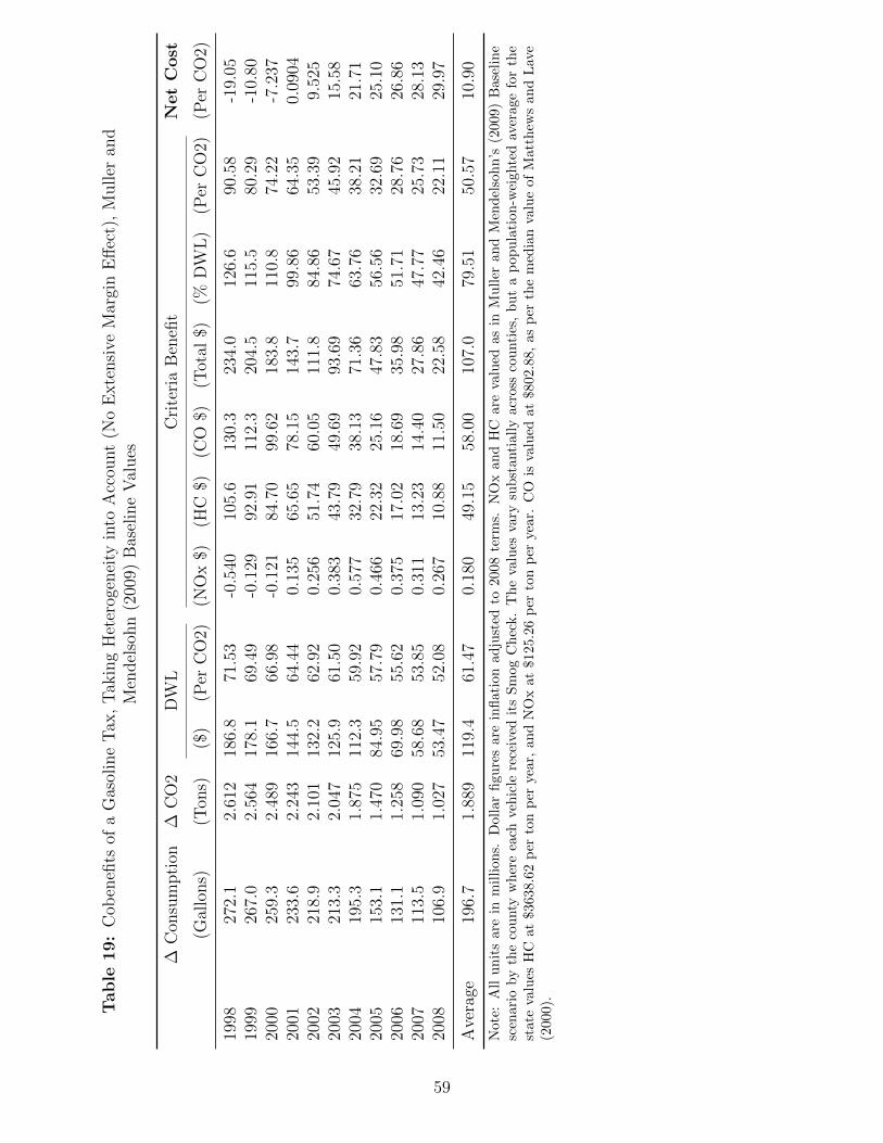
Table
19:
Cob
enefi
tsof
aG
asol
ine
Tax
,T
akin
gH
eter
ogen
eity
into
Acc
ount
(No
Exte
nsi
veM
argi
nE
ffec
t),
Muller
and
Men
del
sohn
(200
9)B
asel
ine
Val
ues
∆C
onsu
mpti
on∆
CO
2D
WL
Cri
teri
aB
enefi
tN
et
Cost
(Gal
lons)
(Ton
s)($
)(P
erC
O2)
(NO
x$)
(HC
$)(C
O$)
(Tot
al$)
(%D
WL
)(P
erC
O2)
(Per
CO
2)
1998
272.
12.
612
186.
871
.53
-0.5
4010
5.6
130.
323
4.0
126.
690
.58
-19.
0519
9926
7.0
2.56
417
8.1
69.4
9-0
.129
92.9
111
2.3
204.
511
5.5
80.2
9-1
0.80
2000
259.
32.
489
166.
766
.98
-0.1
2184
.70
99.6
218
3.8
110.
874
.22
-7.2
3720
0123
3.6
2.24
314
4.5
64.4
40.
135
65.6
578
.15
143.
799
.86
64.3
50.
0904
2002
218.
92.
101
132.
262
.92
0.25
651
.74
60.0
511
1.8
84.8
653
.39
9.52
520
0321
3.3
2.04
712
5.9
61.5
00.
383
43.7
949
.69
93.6
974
.67
45.9
215
.58
2004
195.
31.
875
112.
359
.92
0.57
732
.79
38.1
371
.36
63.7
638
.21
21.7
120
0515
3.1
1.47
084
.95
57.7
90.
466
22.3
225
.16
47.8
356
.56
32.6
925
.10
2006
131.
11.
258
69.9
855
.62
0.37
517
.02
18.6
935
.98
51.7
128
.76
26.8
620
0711
3.5
1.09
058
.68
53.8
50.
311
13.2
314
.40
27.8
647
.77
25.7
328
.13
2008
106.
91.
027
53.4
752
.08
0.26
710
.88
11.5
022
.58
42.4
622
.11
29.9
7
Ave
rage
196.
71.
889
119.
461
.47
0.18
049
.15
58.0
010
7.0
79.5
150
.57
10.9
0
Not
e:A
llu
nit
sar
ein
mil
lion
s.D
olla
rfi
gure
sare
infl
ati
on
ad
just
edto
2008
term
s.N
Ox
an
dH
Care
valu
edas
inM
ull
eran
dM
end
elso
hn
’s(2
009)
Base
lin
esc
enar
ioby
the
cou
nty
wh
ere
each
veh
icle
rece
ived
its
Sm
og
Ch
eck.
Th
eva
lues
vary
sub
stanti
all
yacr
oss
cou
nti
es,
bu
ta
pop
ula
tion
-wei
ghte
dav
erage
for
the
stat
eva
lues
HC
at$3
638.
62p
erto
np
erye
ar,
and
NO
xat
$125.2
6p
erto
np
erye
ar.
CO
isva
lued
at
$802.8
8,as
per
the
med
ian
valu
eof
Matt
hew
san
dL
ave
(200
0).
59
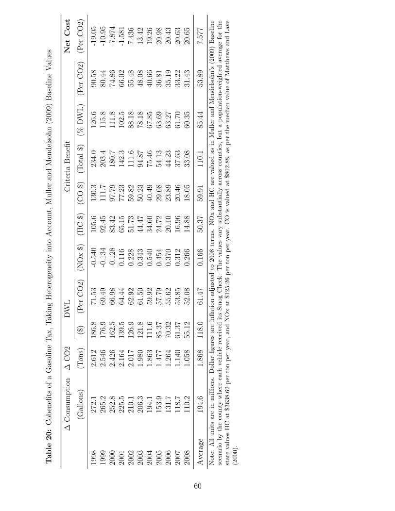
Table
20:
Cob
enefi
tsof
aG
asol
ine
Tax
,T
akin
gH
eter
ogen
eity
into
Acc
ount,
Muller
and
Men
del
sohn
(200
9)B
asel
ine
Val
ues
∆C
onsu
mpti
on∆
CO
2D
WL
Cri
teri
aB
enefi
tN
et
Cost
(Gal
lons)
(Ton
s)($
)(P
erC
O2)
(NO
x$)
(HC
$)(C
O$)
(Tot
al$)
(%D
WL
)(P
erC
O2)
(Per
CO
2)
1998
272.
12.
612
186.
871
.53
-0.5
4010
5.6
130.
323
4.0
126.
690
.58
-19.
0519
9926
5.2
2.54
617
6.9
69.4
9-0
.134
92.4
511
1.7
203.
411
5.8
80.4
4-1
0.95
2000
252.
82.
426
162.
566
.98
-0.1
2883
.42
97.7
918
0.7
111.
874
.86
-7.8
7420
0122
5.5
2.16
413
9.5
64.4
40.
116
65.1
577
.23
142.
310
2.5
66.0
2-1
.581
2002
210.
12.
017
126.
962
.92
0.22
851
.73
59.8
211
1.6
88.1
855
.48
7.43
620
0320
6.3
1.98
012
1.8
61.5
00.
343
44.4
750
.23
94.8
778
.18
48.0
813
.42
2004
194.
11.
863
111.
659
.92
0.54
034
.60
40.4
975
.46
67.8
540
.66
19.2
620
0515
3.9
1.47
785
.37
57.7
90.
454
24.7
229
.08
54.1
363
.69
36.8
120
.98
2006
131.
71.
264
70.3
255
.62
0.37
020
.10
23.8
944
.23
63.2
735
.19
20.4
320
0711
8.7
1.14
061
.37
53.8
50.
312
16.9
620
.46
37.6
361
.70
33.2
220
.63
2008
110.
21.
058
55.1
252
.08
0.26
614
.88
18.0
533
.08
60.3
531
.43
20.6
5
Ave
rage
194.
61.
868
118.
061
.47
0.16
650
.37
59.9
111
0.1
85.4
453
.89
7.57
7
Not
e:A
llu
nit
sar
ein
mil
lion
s.D
olla
rfi
gure
sare
infl
ati
on
ad
just
edto
2008
term
s.N
Ox
an
dH
Care
valu
edas
inM
ull
eran
dM
end
elso
hn
’s(2
009)
Base
lin
esc
enar
ioby
the
cou
nty
wh
ere
each
veh
icle
rece
ived
its
Sm
og
Ch
eck.
Th
eva
lues
vary
sub
stanti
all
yacr
oss
cou
nti
es,
bu
ta
pop
ula
tion
-wei
ghte
dav
erage
for
the
stat
eva
lues
HC
at$3
638.
62p
erto
np
erye
ar,
and
NO
xat
$125.2
6p
erto
np
erye
ar.
CO
isva
lued
at
$802.8
8,as
per
the
med
ian
valu
eof
Matt
hew
san
dL
ave
(200
0).
60
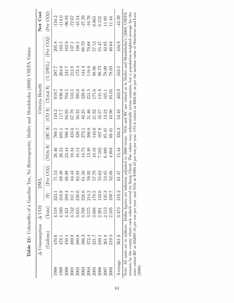
Table
21:
Cob
enefi
tsof
aG
asol
ine
Tax
,N
oH
eter
ogen
eity
,M
uller
and
Men
del
sohn
(200
9)U
SE
PA
Val
ues
∆C
onsu
mpti
on∆
CO
2D
WL
Cri
teri
aB
enefi
tN
et
Cost
(Gal
lons)
(Ton
s)($
)(P
erC
O2)
(NO
x$)
(HC
$)(C
O$)
(Tot
al$)
(%D
WL
)(P
erC
O2)
(Per
CO
2)
1998
470.
64.
518
323.
171
.53
26.4
676
0.5
134.
291
9.7
287.
720
5.8
-134
.219
9947
8.1
4.58
931
8.9
69.4
928
.24
691.
111
7.7
836.
426
4.0
183.
5-1
14.0
2000
450.
14.
321
289.
466
.98
23.4
458
6.4
94.9
570
4.5
244.
716
3.9
-96.
9320
0138
9.8
3.74
224
1.1
64.4
418
.34
424.
667
.78
510.
521
2.8
137.
1-7
2.67
2002
380.
83.
655
230.
062
.92
16.1
432
8.7
50.3
239
5.0
172.
410
8.5
-45.
5420
0338
6.3
3.70
822
8.0
61.5
014
.75
273.
140
.25
328.
014
4.4
88.7
9-2
7.29
2004
372.
43.
575
214.
259
.92
13.4
020
6.8
31.4
625
1.5
118.
070
.68
-10.
7620
0532
1.7
3.08
817
8.5
57.7
910
.18
143.
621
.92
175.
698
.86
57.1
30.
663
2006
249.
12.
391
133.
055
.62
7.58
210
7.8
16.5
713
1.8
99.7
355
.47
0.15
220
0726
1.8
2.51
313
5.3
53.8
56.
480
85.4
113
.22
105.
178
.09
42.0
511
.80
2008
219.
32.
105
109.
752
.08
4.80
469
.41
10.9
085
.05
78.0
340
.64
11.4
4
Ave
rage
361.
83.
473
218.
361
.47
15.4
433
4.3
54.4
840
3.9
163.
510
4.9
-43.
39
Not
e:A
llu
nit
sar
ein
mil
lion
s.D
olla
rfi
gure
sare
infl
ati
on
ad
just
edto
2008
term
s.N
Ox
an
dH
Care
valu
edas
inM
ull
eran
dM
end
elso
hn
’s(2
009)
USE
PA
scen
ario
by
the
cou
nty
wh
ere
each
veh
icle
rece
ived
its
Sm
og
Ch
eck.
Th
eva
lues
vary
sub
stanti
all
yacr
oss
cou
nti
es,
bu
ta
pop
ula
tion
-wei
ghte
dav
erage
for
the
stat
eva
lues
HC
at$2
3897
.10
per
ton
per
year
,an
dN
Ox
at
$1995.4
3p
erto
np
erye
ar.
CO
isva
lued
at
$802.8
8,
as
per
the
med
ian
valu
eof
Matt
hew
san
dL
ave
(200
0).
61
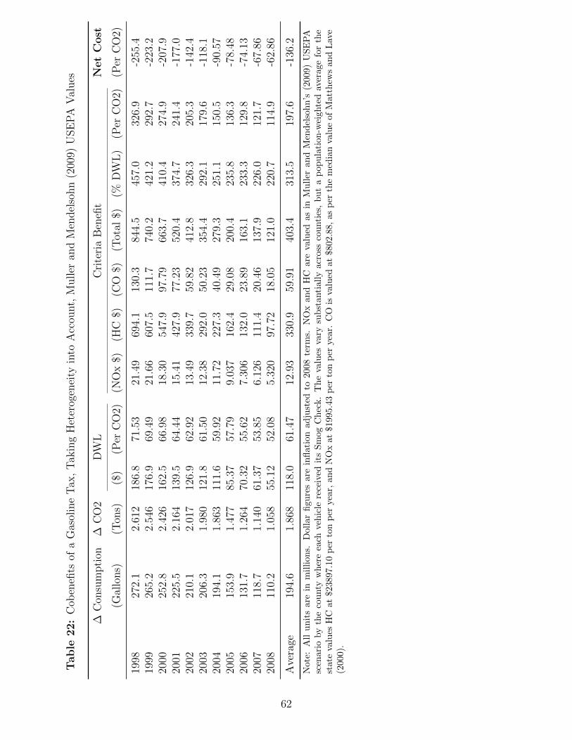
Table
22:
Cob
enefi
tsof
aG
asol
ine
Tax
,T
akin
gH
eter
ogen
eity
into
Acc
ount,
Muller
and
Men
del
sohn
(200
9)U
SE
PA
Val
ues
∆C
onsu
mpti
on∆
CO
2D
WL
Cri
teri
aB
enefi
tN
et
Cost
(Gal
lons)
(Ton
s)($
)(P
erC
O2)
(NO
x$)
(HC
$)(C
O$)
(Tot
al$)
(%D
WL
)(P
erC
O2)
(Per
CO
2)
1998
272.
12.
612
186.
871
.53
21.4
969
4.1
130.
384
4.5
457.
032
6.9
-255
.419
9926
5.2
2.54
617
6.9
69.4
921
.66
607.
511
1.7
740.
242
1.2
292.
7-2
23.2
2000
252.
82.
426
162.
566
.98
18.3
054
7.9
97.7
966
3.7
410.
427
4.9
-207
.920
0122
5.5
2.16
413
9.5
64.4
415
.41
427.
977
.23
520.
437
4.7
241.
4-1
77.0
2002
210.
12.
017
126.
962
.92
13.4
933
9.7
59.8
241
2.8
326.
320
5.3
-142
.420
0320
6.3
1.98
012
1.8
61.5
012
.38
292.
050
.23
354.
429
2.1
179.
6-1
18.1
2004
194.
11.
863
111.
659
.92
11.7
222
7.3
40.4
927
9.3
251.
115
0.5
-90.
5720
0515
3.9
1.47
785
.37
57.7
99.
037
162.
429
.08
200.
423
5.8
136.
3-7
8.48
2006
131.
71.
264
70.3
255
.62
7.30
613
2.0
23.8
916
3.1
233.
312
9.8
-74.
1320
0711
8.7
1.14
061
.37
53.8
56.
126
111.
420
.46
137.
922
6.0
121.
7-6
7.86
2008
110.
21.
058
55.1
252
.08
5.32
097
.72
18.0
512
1.0
220.
711
4.9
-62.
86
Ave
rage
194.
61.
868
118.
061
.47
12.9
333
0.9
59.9
140
3.4
313.
519
7.6
-136
.2
Not
e:A
llu
nit
sar
ein
mil
lion
s.D
olla
rfi
gure
sare
infl
ati
on
ad
just
edto
2008
term
s.N
Ox
an
dH
Care
valu
edas
inM
ull
eran
dM
end
elso
hn
’s(2
009)
USE
PA
scen
ario
by
the
cou
nty
wh
ere
each
veh
icle
rece
ived
its
Sm
og
Ch
eck.
Th
eva
lues
vary
sub
stanti
all
yacr
oss
cou
nti
es,
bu
ta
pop
ula
tion
-wei
ghte
dav
erage
for
the
stat
eva
lues
HC
at$2
3897
.10
per
ton
per
year
,an
dN
Ox
at
$1995.4
3p
erto
np
erye
ar.
CO
isva
lued
at
$802.8
8,
as
per
the
med
ian
valu
eof
Matt
hew
san
dL
ave
(200
0).
62
A Steps to clean smog check data
A.1 Smog Check Data
Our data from the Smog Check Program are essentially the universe of test records from
January 1, 1996 to December 31, 2010. We were only able to obtain test records going back
to 1996 because this was the year when the Smog Check program introduced its electronic
transmission system. Because the system seems to have been phased in during the first half of
1996, and major program changes took effect in 1998 we limit our sample to test records from
January 1998 on. For our analyses, we use a 10% sample of VINs, selecting by the second to
last digit of the VIN. We exclude tests which have no odometer reading, with a test result
of ”Tampered” or ”Aborted” and vehicles which have more than 36 tests in the span of the
data. Vehicles often have multiple Smog Check records in a year, whether due to changes of
ownership or failed tests, but we argue that more than 36 in what is at most a 12 year-span
indicates some problem with the data.22
A few adjustments must be made to accurately estimate VMT and emissions per mile.
First, we adjust odometer readings for roll-overs and typos. Many of the vehicles in our
analysis were manufacturer withe 5-digit odometers–that is, five places for whole numbers plus
a decimal. As such, any time one of these vehicles crosses over 100,000 miles, the odometer
“rolls over” back to 0. To complicate matters further, sometimes either the vehicle owner
or Smog Check technician notices this problem and records the appropriate number in the
100,000s place, and sometimes they do not. To address this problem, we employ an algorithm
that increases the hundred thousands place in the odometer reading whenever a rollover seems
to have occurred. The hundred thousands are incremented if the previous test record shows
higher mileage, or if the next test record is shows more than 100,000 additional miles on the
odometer (indicating that the odometer had already rolled over, but the next check took this
into account). The algorithm also attempts to correct for typos and entry errors. An odometer
reading is flagged if it does not fit with surrounding readings for the same vehicle–either it
is less than the previous reading or greater the next–and cannot be explained by a rollover.
The algorithm then tests whether fixing one of several common typos will make the flagged
22For instance, there is one vehicle in particular, a 1986 Volvo station wagon, which has records for morethan 600 Smog Checks between January 1996 and March 1998. The vehicle likely belonged to a Smog Checktechnician who used it to test the electronic transmission system.
63
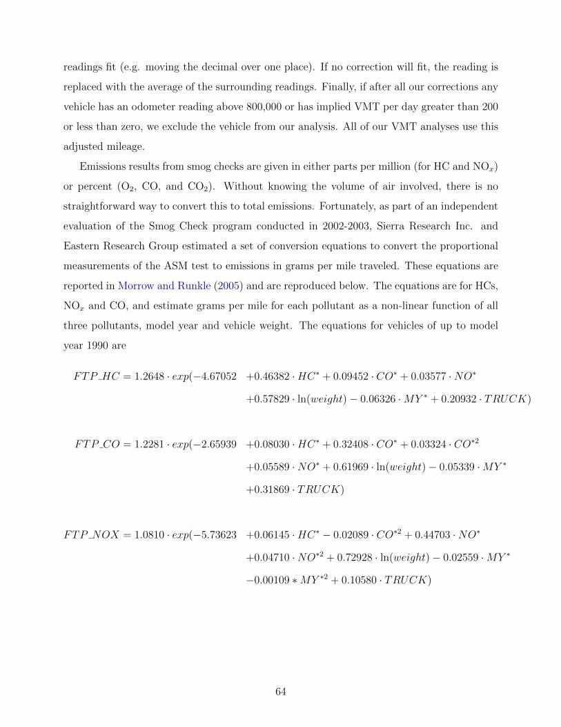
readings fit (e.g. moving the decimal over one place). If no correction will fit, the reading is
replaced with the average of the surrounding readings. Finally, if after all our corrections any
vehicle has an odometer reading above 800,000 or has implied VMT per day greater than 200
or less than zero, we exclude the vehicle from our analysis. All of our VMT analyses use this
adjusted mileage.
Emissions results from smog checks are given in either parts per million (for HC and NOx)
or percent (O2, CO, and CO2). Without knowing the volume of air involved, there is no
straightforward way to convert this to total emissions. Fortunately, as part of an independent
evaluation of the Smog Check program conducted in 2002-2003, Sierra Research Inc. and
Eastern Research Group estimated a set of conversion equations to convert the proportional
measurements of the ASM test to emissions in grams per mile traveled. These equations are
reported in Morrow and Runkle (2005) and are reproduced below. The equations are for HCs,
NOx and CO, and estimate grams per mile for each pollutant as a non-linear function of all
three pollutants, model year and vehicle weight. The equations for vehicles of up to model
year 1990 are
FTP HC = 1.2648 · exp(−4.67052 +0.46382 ·HC∗ + 0.09452 · CO∗ + 0.03577 ·NO∗
+0.57829 · ln(weight)− 0.06326 ·MY ∗ + 0.20932 · TRUCK)
FTP CO = 1.2281 · exp(−2.65939 +0.08030 ·HC∗ + 0.32408 · CO∗ + 0.03324 · CO∗2
+0.05589 ·NO∗ + 0.61969 · ln(weight)− 0.05339 ·MY ∗
+0.31869 · TRUCK)
FTP NOX = 1.0810 · exp(−5.73623 +0.06145 ·HC∗ − 0.02089 · CO∗2 + 0.44703 ·NO∗
+0.04710 ·NO∗2 + 0.72928 · ln(weight)− 0.02559 ·MY ∗
−0.00109 ∗MY ∗2 + 0.10580 · TRUCK)
64
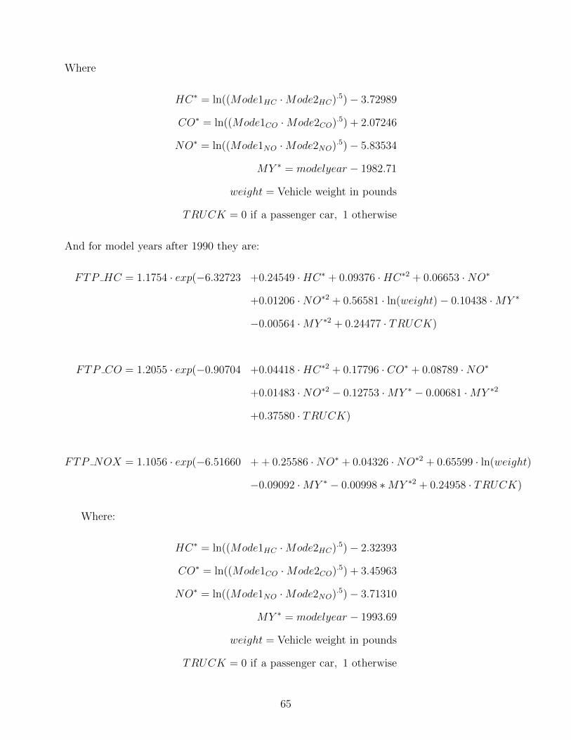
Where
HC∗ = ln((Mode1HC ·Mode2HC).5)− 3.72989
CO∗ = ln((Mode1CO ·Mode2CO).5) + 2.07246
NO∗ = ln((Mode1NO ·Mode2NO).5)− 5.83534
MY ∗ = modelyear − 1982.71
weight = Vehicle weight in pounds
TRUCK = 0 if a passenger car, 1 otherwise
And for model years after 1990 they are:
FTP HC = 1.1754 · exp(−6.32723 +0.24549 ·HC∗ + 0.09376 ·HC∗2 + 0.06653 ·NO∗
+0.01206 ·NO∗2 + 0.56581 · ln(weight)− 0.10438 ·MY ∗
−0.00564 ·MY ∗2 + 0.24477 · TRUCK)
FTP CO = 1.2055 · exp(−0.90704 +0.04418 ·HC∗2 + 0.17796 · CO∗ + 0.08789 ·NO∗
+0.01483 ·NO∗2 − 0.12753 ·MY ∗ − 0.00681 ·MY ∗2
+0.37580 · TRUCK)
FTP NOX = 1.1056 · exp(−6.51660 + + 0.25586 ·NO∗ + 0.04326 ·NO∗2 + 0.65599 · ln(weight)
−0.09092 ·MY ∗ − 0.00998 ∗MY ∗2 + 0.24958 · TRUCK)
Where:
HC∗ = ln((Mode1HC ·Mode2HC).5)− 2.32393
CO∗ = ln((Mode1CO ·Mode2CO).5) + 3.45963
NO∗ = ln((Mode1NO ·Mode2NO).5)− 3.71310
MY ∗ = modelyear − 1993.69
weight = Vehicle weight in pounds
TRUCK = 0 if a passenger car, 1 otherwise
65
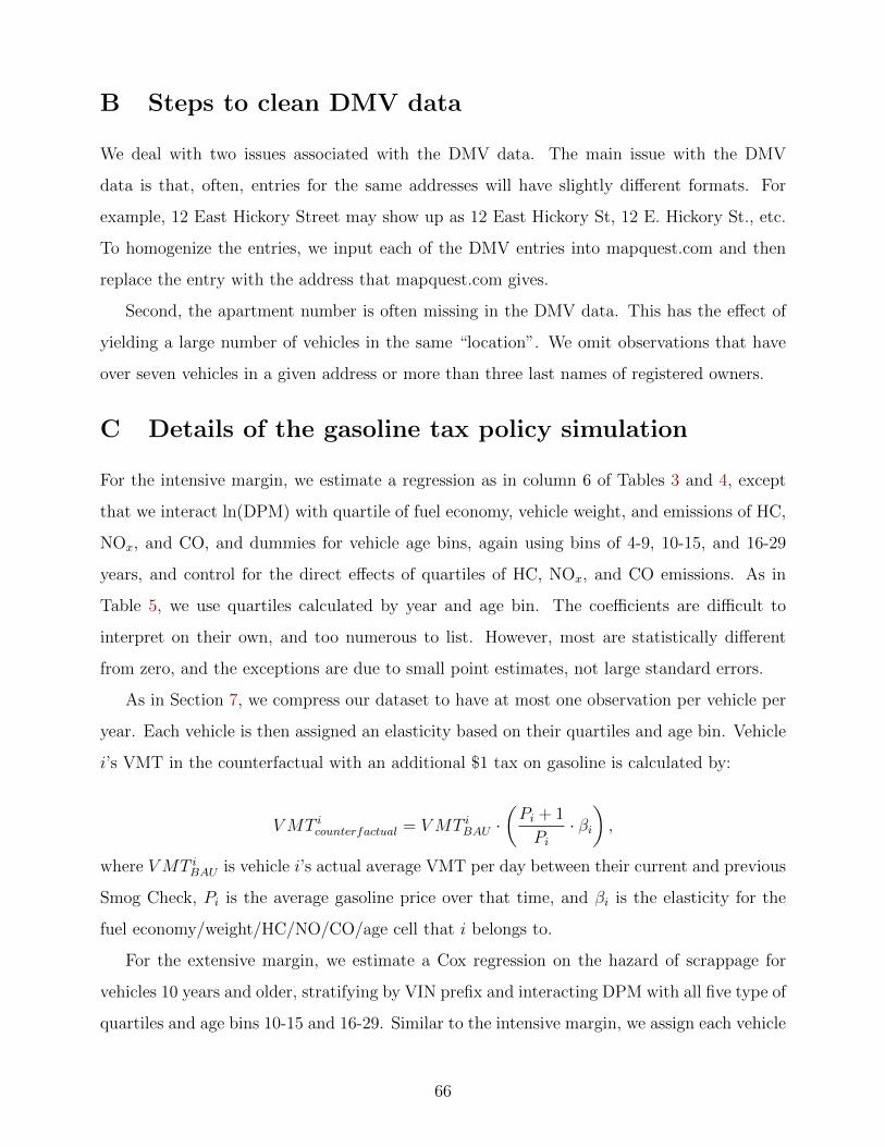
B Steps to clean DMV data
We deal with two issues associated with the DMV data. The main issue with the DMV
data is that, often, entries for the same addresses will have slightly different formats. For
example, 12 East Hickory Street may show up as 12 East Hickory St, 12 E. Hickory St., etc.
To homogenize the entries, we input each of the DMV entries into mapquest.com and then
replace the entry with the address that mapquest.com gives.
Second, the apartment number is often missing in the DMV data. This has the effect of
yielding a large number of vehicles in the same “location”. We omit observations that have
over seven vehicles in a given address or more than three last names of registered owners.
C Details of the gasoline tax policy simulation
For the intensive margin, we estimate a regression as in column 6 of Tables 3 and 4, except
that we interact ln(DPM) with quartile of fuel economy, vehicle weight, and emissions of HC,
NOx, and CO, and dummies for vehicle age bins, again using bins of 4-9, 10-15, and 16-29
years, and control for the direct effects of quartiles of HC, NOx, and CO emissions. As in
Table 5, we use quartiles calculated by year and age bin. The coefficients are difficult to
interpret on their own, and too numerous to list. However, most are statistically different
from zero, and the exceptions are due to small point estimates, not large standard errors.
As in Section 7, we compress our dataset to have at most one observation per vehicle per
year. Each vehicle is then assigned an elasticity based on their quartiles and age bin. Vehicle
i’s VMT in the counterfactual with an additional $1 tax on gasoline is calculated by:
VMT icounterfactual = VMT iBAU ·(Pi + 1
Pi· βi),
where VMT iBAU is vehicle i’s actual average VMT per day between their current and previous
Smog Check, Pi is the average gasoline price over that time, and βi is the elasticity for the
fuel economy/weight/HC/NO/CO/age cell that i belongs to.
For the extensive margin, we estimate a Cox regression on the hazard of scrappage for
vehicles 10 years and older, stratifying by VIN prefix and interacting DPM with all five type of
quartiles and age bins 10-15 and 16-29. Similar to the intensive margin, we assign each vehicle
66
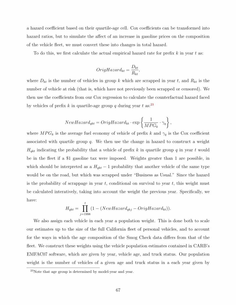
a hazard coefficient based on their quartile-age cell. Cox coefficients can be transformed into
hazard ratios, but to simulate the affect of an increase in gasoline prices on the composition
of the vehicle fleet, we must convert these into changes in total hazard.
To do this, we first calculate the actual empirical hazard rate for prefix k in year t as:
OrigHazardkt =Dkt
Rkt
,
where Dkt is the number of vehicles in group k which are scrapped in year t, and Rkt is the
number of vehicle at risk (that is, which have not previously been scrapped or censored). We
then use the coefficients from our Cox regression to calculate the counterfactual hazard faced
by vehicles of prefix k in quartile-age group q during year t as:23
NewHazardqkt = OrigHazardkt · exp
{1
MPGk
· γq},
where MPGk is the average fuel economy of vehicle of prefix k and γq is the Cox coefficient
associated with quartile group q. We then use the change in hazard to construct a weight
Hqkt indicating the probability that a vehicle of prefix k in quartile group q in year t would
be in the fleet if a $1 gasoline tax were imposed. Weights greater than 1 are possible, in
which should be interpreted as a Hqkt − 1 probability that another vehicle of the same type
would be on the road, but which was scrapped under “Business as Usual.” Since the hazard
is the probability of scrappage in year t, conditional on survival to year t, this weight must
be calculated interatively, taking into account the weight the previous year. Specifically, we
have:
Hqkt =t∏
j=1998
(1− (NewHazardqkj −OrigHazardkt)).
We also assign each vehicle in each year a population weight. This is done both to scale
our estimates up to the size of the full California fleet of personal vehicles, and to account
for the ways in which the age composition of the Smog Check data differs from that of the
fleet. We construct these weights using the vehicle population estimates contained in CARB’s
EMFAC07 software, which are given by year, vehicle age, and truck status. Our population
weight is the number of vehicles of a given age and truck status in a each year given by
23Note that age group is determined by model-year and year.
67
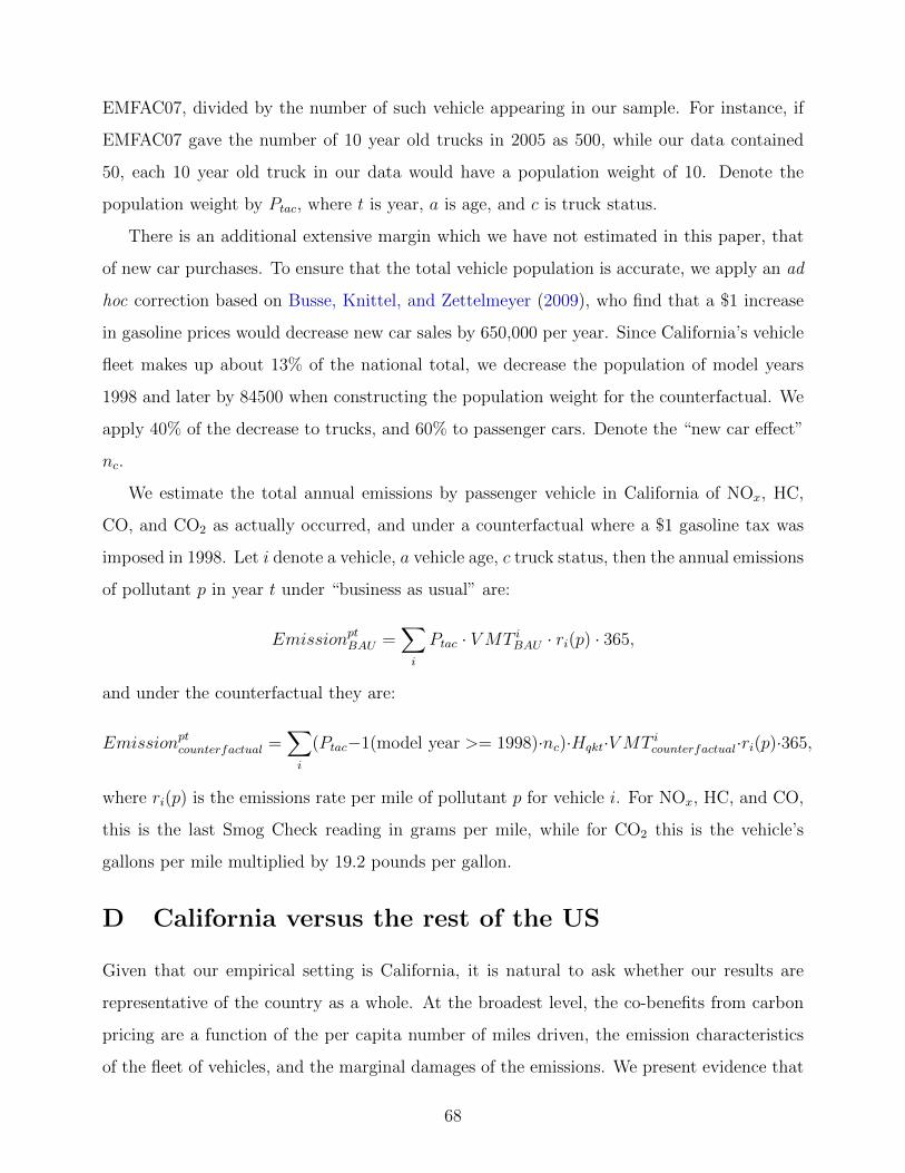
EMFAC07, divided by the number of such vehicle appearing in our sample. For instance, if
EMFAC07 gave the number of 10 year old trucks in 2005 as 500, while our data contained
50, each 10 year old truck in our data would have a population weight of 10. Denote the
population weight by Ptac, where t is year, a is age, and c is truck status.
There is an additional extensive margin which we have not estimated in this paper, that
of new car purchases. To ensure that the total vehicle population is accurate, we apply an ad
hoc correction based on Busse, Knittel, and Zettelmeyer (2009), who find that a $1 increase
in gasoline prices would decrease new car sales by 650,000 per year. Since California’s vehicle
fleet makes up about 13% of the national total, we decrease the population of model years
1998 and later by 84500 when constructing the population weight for the counterfactual. We
apply 40% of the decrease to trucks, and 60% to passenger cars. Denote the “new car effect”
nc.
We estimate the total annual emissions by passenger vehicle in California of NOx, HC,
CO, and CO2 as actually occurred, and under a counterfactual where a $1 gasoline tax was
imposed in 1998. Let i denote a vehicle, a vehicle age, c truck status, then the annual emissions
of pollutant p in year t under “business as usual” are:
EmissionptBAU =∑i
Ptac · VMT iBAU · ri(p) · 365,
and under the counterfactual they are:
Emissionptcounterfactual =∑i
(Ptac−1(model year >= 1998)·nc)·Hqkt·VMT icounterfactual·ri(p)·365,
where ri(p) is the emissions rate per mile of pollutant p for vehicle i. For NOx, HC, and CO,
this is the last Smog Check reading in grams per mile, while for CO2 this is the vehicle’s
gallons per mile multiplied by 19.2 pounds per gallon.
D California versus the rest of the US
Given that our empirical setting is California, it is natural to ask whether our results are
representative of the country as a whole. At the broadest level, the co-benefits from carbon
pricing are a function of the per capita number of miles driven, the emission characteristics
of the fleet of vehicles, and the marginal damages of the emissions. We present evidence that
68

the benefits may, in fact, be larger outside of California. The reason for this is that while
the marginal damages are indeed larger in California, the vehicle stock in California is much
cleaner than the rest of the country because California has traditionally lead the rest of the
US in terms of vehicle emission standards.
The results in Muller and Mendelsohn (2009) provide a convenient way to test whether
California differs in terms of marginal damages. Table A.25 presents points on the distribution
of marginal damages for NOx, HCs, and the sum of the two, weighted by each county’s annual
VMT.24 Figure A.11 plots the kernel density estimates of the distributions. We present the
sum of because counties are typically either “NOx constrained” or “VOC (HC) constrained”
and the sum is perhaps more informative. As expected, the marginal damages are higher in
California for HCs, but lower for NOx, as California counties tend to be VOC-constrained.
The sum of the two marginal damages is 78 percent higher in California. Higher points in the
distribution show an even larger disparity.
This effect is offset, however, by the cleaner vehicle stock within California—a result of
California’s stricter emission standards. To illustrate this, we collected county-level average
per-mile emission rates for NOx, HCs, and CO from the EPA Motor Vehicle Emission Simula-
tor (MOVES). This reports total emissions from transportation and annual mileage for each
county. Table A.25 also presents points on the per-mile emissions and Figure A.12 plots the
distributions.25 Mean county-level NOx, HCs, and CO are 67, 36, and 31 percent lower in
California, respectively. Other points in the distributions exhibit similar patterns.
Finally, we calculate the county-level average per-mile externality for each pollutant, as
well as the sum of the three. Table A.25 and Figure A.13 illustrates these. As expected the
HC damages are higher, but the average county-level per-mile externality from the sum the
three pollutants is 30 percent lower in California compared to the rest of the country; the
25th percentile, median, and 75th percentile are 35, 30, and 9 percent lower, respectively.
These calculations suggest that, provided the average VMT elasticities are not significantly
smaller outside of California and/or the heterogeneity across vehicle types is not significantly
24All of the points on the distribution and densities discussed in this section weight each county by its totalVMT.
25We note that these are higher than the averages in our data. This may reflect the fact that smog checksare not required for vehicles with model years before 1975 and these vehicles likely have very high emissionssince this pre-dates many of the emission standards within the US.
69

different (in the reverse way), our estimates are likely to apply to the rest of the country.
70
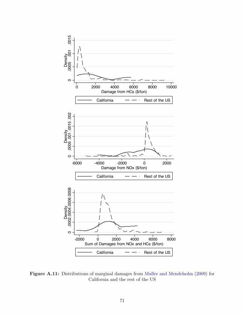
0.0
005
.001
.001
5De
nsity
0 2000 4000 6000 8000 10000Damage from HCs ($/ton)
California Rest of the US
0.0
005
.001
.001
5.0
02De
nsity
-6000 -4000 -2000 0 2000Damage from NOx ($/ton)
California Rest of the US
0.0
002.
0004
.000
6.00
08De
nsity
-2000 0 2000 4000 6000 8000Sum of Damages from NOx and HCs ($/ton)
California Rest of the US
Figure A.11: Distributions of marginal damages from Muller and Mendelsohn (2009) forCalifornia and the rest of the US
71
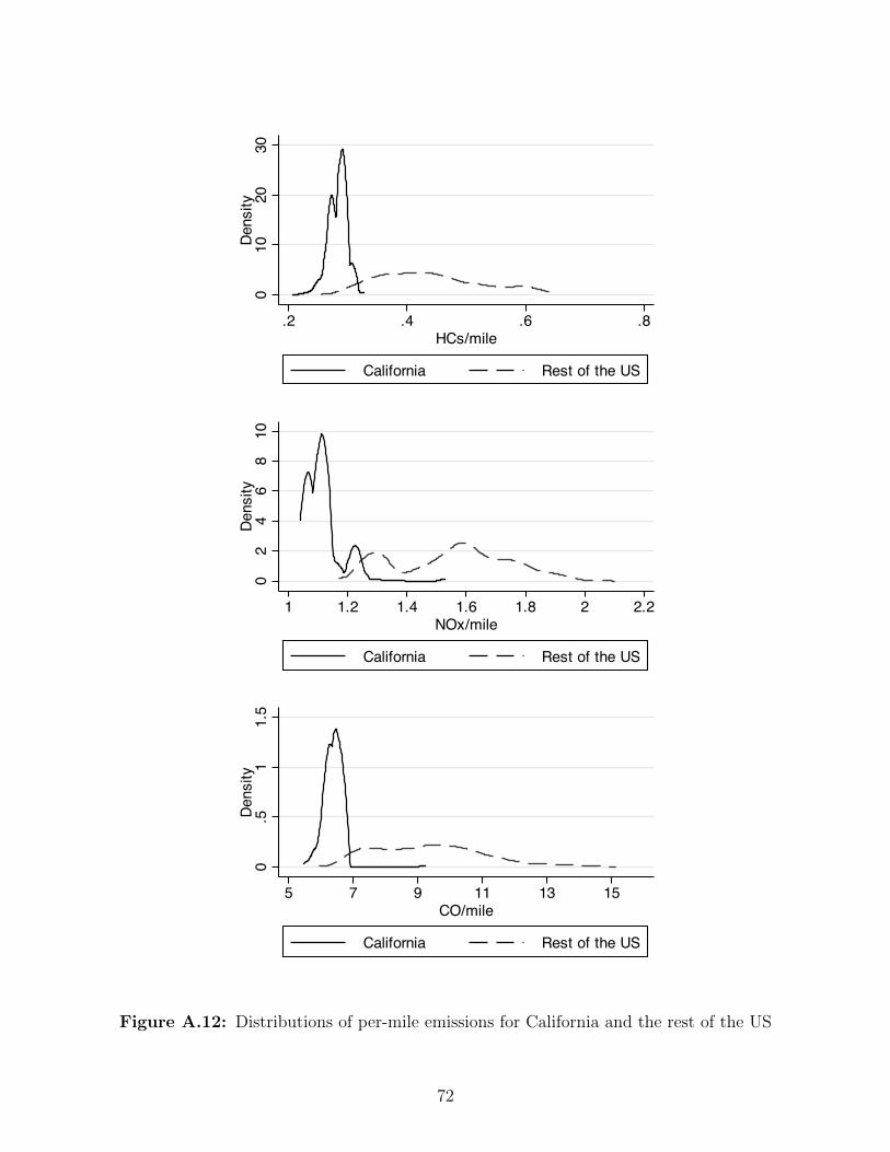
010
2030
Dens
ity
.2 .4 .6 .8HCs/mile
California Rest of the US
02
46
810
Dens
ity
1 1.2 1.4 1.6 1.8 2 2.2NOx/mile
California Rest of the US
0.5
11.
5De
nsity
5 7 9 11 13 15CO/mile
California Rest of the US
Figure A.12: Distributions of per-mile emissions for California and the rest of the US
72
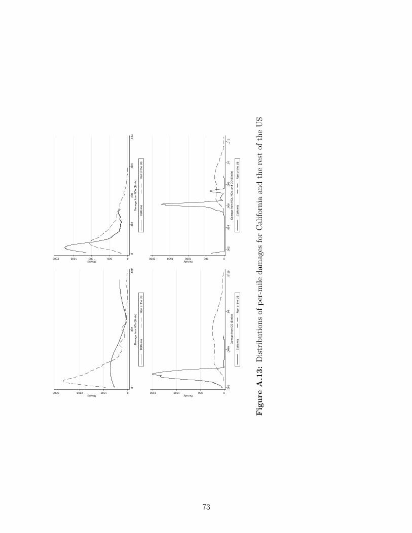
0100020003000Density
0.0
01.0
02Da
mag
e fro
m H
Cs ($
/mile
)
Califo
rnia
Rest
of t
he U
S
0500100015002000Density
0.0
01.0
02.0
03.0
04Da
mag
e fro
m N
Ox
($/m
ile)
Califo
rnia
Rest
of t
he U
S050010001500
Density
.005
.007
5.0
1.0
125
Dam
age
from
CO
($/m
ile)
Califo
rnia
Rest
of t
he U
S
0500100015002000Density
.002
.004
.006
.008
.01
.012
Dam
age
from
HCs
, NO
x, a
nd C
O ($
/mile
)
Califo
rnia
Rest
of t
he U
S
Fig
ure
A.1
3:
Dis
trib
uti
ons
ofp
er-m
ile
dam
ages
for
Cal
ifor
nia
and
the
rest
ofth
eU
S
73
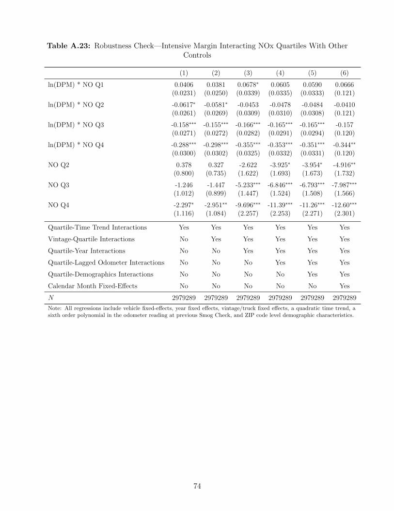
Table A.23: Robustness Check—Intensive Margin Interacting NOx Quartiles With OtherControls
(1) (2) (3) (4) (5) (6)
ln(DPM) * NO Q1 0.0406 0.0381 0.0678∗ 0.0605 0.0590 0.0666(0.0231) (0.0250) (0.0339) (0.0335) (0.0333) (0.121)
ln(DPM) * NO Q2 -0.0617∗ -0.0581∗ -0.0453 -0.0478 -0.0484 -0.0410(0.0261) (0.0269) (0.0309) (0.0310) (0.0308) (0.121)
ln(DPM) * NO Q3 -0.158∗∗∗ -0.155∗∗∗ -0.166∗∗∗ -0.165∗∗∗ -0.165∗∗∗ -0.157(0.0271) (0.0272) (0.0282) (0.0291) (0.0294) (0.120)
ln(DPM) * NO Q4 -0.288∗∗∗ -0.298∗∗∗ -0.355∗∗∗ -0.353∗∗∗ -0.351∗∗∗ -0.344∗∗
(0.0300) (0.0302) (0.0325) (0.0332) (0.0331) (0.120)
NO Q2 0.378 0.327 -2.622 -3.925∗ -3.954∗ -4.916∗∗
(0.800) (0.735) (1.622) (1.693) (1.673) (1.732)
NO Q3 -1.246 -1.447 -5.233∗∗∗ -6.846∗∗∗ -6.793∗∗∗ -7.987∗∗∗
(1.012) (0.899) (1.447) (1.524) (1.508) (1.566)
NO Q4 -2.297∗ -2.951∗∗ -9.696∗∗∗ -11.39∗∗∗ -11.26∗∗∗ -12.60∗∗∗
(1.116) (1.084) (2.257) (2.253) (2.271) (2.301)
Quartile-Time Trend Interactions Yes Yes Yes Yes Yes Yes
Vintage-Quartile Interactions No Yes Yes Yes Yes Yes
Quartile-Year Interactions No No Yes Yes Yes Yes
Quartile-Lagged Odometer Interactions No No No Yes Yes Yes
Quartile-Demographics Interactions No No No No Yes Yes
Calendar Month Fixed-Effects No No No No No Yes
N 2979289 2979289 2979289 2979289 2979289 2979289
Note: All regressions include vehicle fixed-effects, year fixed effects, vintage/truck fixed effects, a quadratic time trend, asixth order polynomial in the odometer reading at previous Smog Check, and ZIP code level demographic characteristics.
74
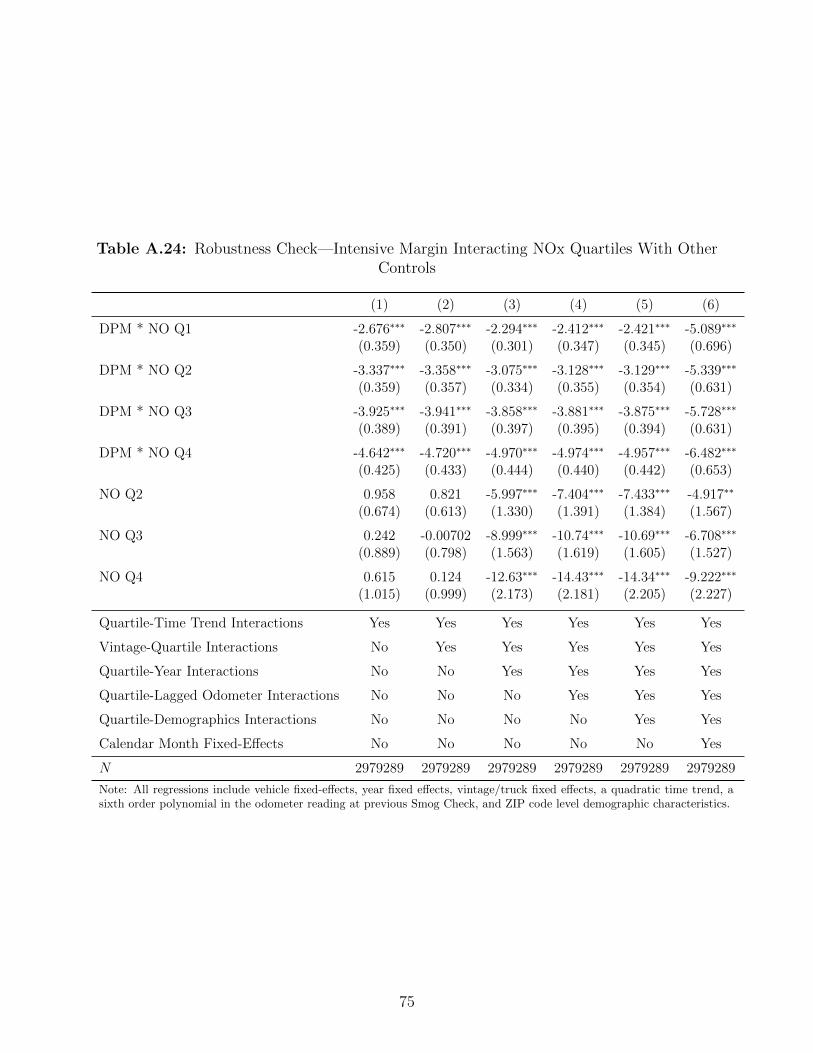
Table A.24: Robustness Check—Intensive Margin Interacting NOx Quartiles With OtherControls
(1) (2) (3) (4) (5) (6)
DPM * NO Q1 -2.676∗∗∗ -2.807∗∗∗ -2.294∗∗∗ -2.412∗∗∗ -2.421∗∗∗ -5.089∗∗∗
(0.359) (0.350) (0.301) (0.347) (0.345) (0.696)
DPM * NO Q2 -3.337∗∗∗ -3.358∗∗∗ -3.075∗∗∗ -3.128∗∗∗ -3.129∗∗∗ -5.339∗∗∗
(0.359) (0.357) (0.334) (0.355) (0.354) (0.631)
DPM * NO Q3 -3.925∗∗∗ -3.941∗∗∗ -3.858∗∗∗ -3.881∗∗∗ -3.875∗∗∗ -5.728∗∗∗
(0.389) (0.391) (0.397) (0.395) (0.394) (0.631)
DPM * NO Q4 -4.642∗∗∗ -4.720∗∗∗ -4.970∗∗∗ -4.974∗∗∗ -4.957∗∗∗ -6.482∗∗∗
(0.425) (0.433) (0.444) (0.440) (0.442) (0.653)
NO Q2 0.958 0.821 -5.997∗∗∗ -7.404∗∗∗ -7.433∗∗∗ -4.917∗∗
(0.674) (0.613) (1.330) (1.391) (1.384) (1.567)
NO Q3 0.242 -0.00702 -8.999∗∗∗ -10.74∗∗∗ -10.69∗∗∗ -6.708∗∗∗
(0.889) (0.798) (1.563) (1.619) (1.605) (1.527)
NO Q4 0.615 0.124 -12.63∗∗∗ -14.43∗∗∗ -14.34∗∗∗ -9.222∗∗∗
(1.015) (0.999) (2.173) (2.181) (2.205) (2.227)
Quartile-Time Trend Interactions Yes Yes Yes Yes Yes Yes
Vintage-Quartile Interactions No Yes Yes Yes Yes Yes
Quartile-Year Interactions No No Yes Yes Yes Yes
Quartile-Lagged Odometer Interactions No No No Yes Yes Yes
Quartile-Demographics Interactions No No No No Yes Yes
Calendar Month Fixed-Effects No No No No No Yes
N 2979289 2979289 2979289 2979289 2979289 2979289
Note: All regressions include vehicle fixed-effects, year fixed effects, vintage/truck fixed effects, a quadratic time trend, asixth order polynomial in the odometer reading at previous Smog Check, and ZIP code level demographic characteristics.
75
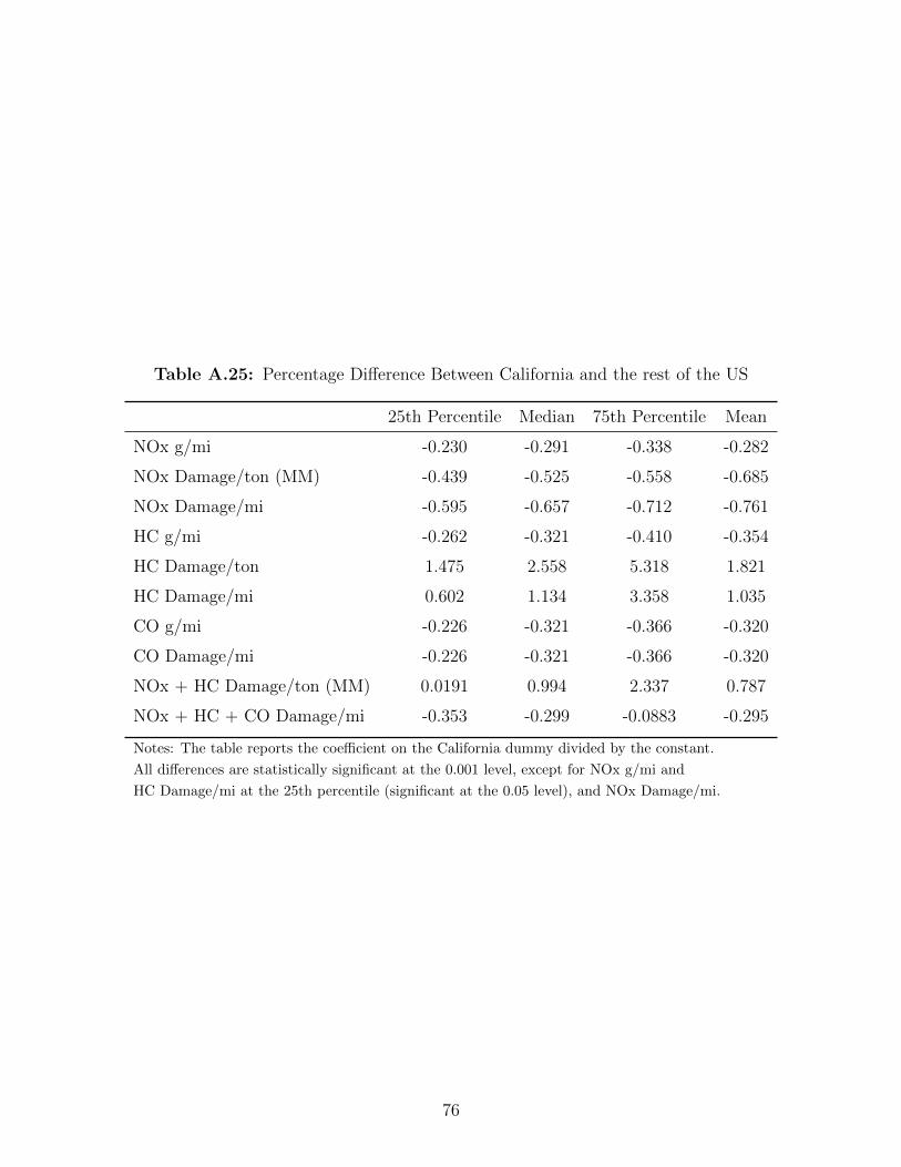
Table A.25: Percentage Difference Between California and the rest of the US
25th Percentile Median 75th Percentile Mean
NOx g/mi -0.230 -0.291 -0.338 -0.282
NOx Damage/ton (MM) -0.439 -0.525 -0.558 -0.685
NOx Damage/mi -0.595 -0.657 -0.712 -0.761
HC g/mi -0.262 -0.321 -0.410 -0.354
HC Damage/ton 1.475 2.558 5.318 1.821
HC Damage/mi 0.602 1.134 3.358 1.035
CO g/mi -0.226 -0.321 -0.366 -0.320
CO Damage/mi -0.226 -0.321 -0.366 -0.320
NOx + HC Damage/ton (MM) 0.0191 0.994 2.337 0.787
NOx + HC + CO Damage/mi -0.353 -0.299 -0.0883 -0.295
Notes: The table reports the coefficient on the California dummy divided by the constant.
All differences are statistically significant at the 0.001 level, except for NOx g/mi and
HC Damage/mi at the 25th percentile (significant at the 0.05 level), and NOx Damage/mi.
76