the determinants of sticky prices and sticky plans: evidence from german business survey data

The Determinants of Sticky Prices andSticky Plans: Evidence from GermanBusiness Survey DataHeike SchenkelbergMunich Graduate School of Economics

Abstract. So far, there is no consensus on the price adjustment determinants in theempirical literature. Analyzing a novel firm-level business survey data set, we providenew insights on the price setting behavior of German retailers during a low inflationperiod. Relating the probability of both price and pricing plan adjustment to time- andstate-dependent variables, we find that state-dependence is important; the macroeco-nomic environment as well as the firm-specific condition significantly determines thetiming of both actual price changes and pricing plan adjustments. Moreover, input costchanges are important determinants of price setting. Finally, price increases respondmore strongly to cost shocks compared to price decreases.

JEL classification: E31, E32, E52.

Keywords: Price setting behavior; time dependent pricing; state dependentpricing; sticky prices; sticky plans.

1. INTRODUCTION

The appropriate modeling of price stickiness has long been a major concernwithin the New-Keynesian literature. In standard time-dependent models, firmsregularly adjust prices independently of the economic environment (Calvo, 1983;Taylor, 1980). Contrarily, state-dependent theories assume the timing of pricechanges to be the outcome of a profit maximization problem of firms; the fre-quency of price adjustment thus varies with the state of the economy.1 Under-standing the exact mechanism underlying price adjustment decisions isimportant because competing models predict divergent effects of monetary policy(Dotsey et al., 1999) and may lead to distinct welfare implications (Lombardo andVestin, 2008). We add to this discussion by analyzing a new dataset compiled bythe Ifo Institute for Economic Research consisting of a large panel of monthlyfirm-level business surveys from 1991:01 to 2006:01. In particular, we estimateunivariate and bivariate probit models to assess the relative importance of time-and state-dependent variables for the probability of both the adjustment of pricesand pricing plans. While in the last years, an increasing empirical literature onprice stickiness at the micro level emerged, results from these studies concerningthe determinants of price adjustment still remain rather inconclusive. Examplesof corresponding studies include Cecchetti (1986) using data on magazine prices

1. See for example Dotsey, et al. (1999), Gertler and Leahy (2008) and Golosov and Lucas (2007).

German Economic Review 15(3): 353–373 doi: 10.1111/geer.12011

© 2013 The AuthorGerman Economic Review © 2013 Verein fur Socialpolitik. Published by Blackwell Publishing Ltd, 9600Garsington Road, Oxford OX4 2DQ, UK and 350 Main Street, Malden, MA 02148, USA.

as well as Bils and Klenow (2004), Klenow and Kryvtsov (2008) and Nakamuraand Steinsson (2008) analyzing larger sets of price data on a broad range of goodscollected by national statistical offices to calculate the consumer-/ producer priceindex (CPI/PPI) for the U.S. Studies for Euro area countries include Rumler et al.(2011), Aucremanne and Dhyne (2005) and Stahl (2010); Dhyne et al. (2006) andVermeulen et al. (2007) summarize results for the Euro area as a whole. One rea-son for the lacking consensus concerning the determinants of price adjustmentmay be that it is generally difficult to fully capture the price setting decision pro-cess at the level of the firm using these quantitative datasets. By contrast, businesssurvey data better allow to analyze pricing behavior at the level of the individualfirm leading to potentially clearer results concerning the price adjustment pro-cess. So far, business survey data has rarely been used to analyze price setting;recent exceptions are Lein (2010) and Loupias and Sevestre (2010) for the Swissand French industrial sector, respectively. For Germany, corresponding businesssurvey evidence has so far not been forthcoming.2

We contribute to the literature on various important dimensions. First, weanalyze whether the price adjustment frequency is determined by time- or state-dependent factors. In contrast to many of the existing studies, we are indeed ableto analyze the determinants of price setting at the level of the individual firmwhen investigating this issue. As stressed above, relative to an assessment at theitem-level, such an analysis has the advantage of explicitly capturing the individ-ual business environment of firms since the data allow matching changes inprices to several other firm characteristics. Thus, arguably, a firm-level assessmententails more direct implications for micro-founded macro models. Furthermore,because the price data can be linked to input costs on a product group-specificbasis, we are able to use the frequency of input price changes as a proxy for priceshocks allowing an explicit analysis of the importance of such shocks for pricesetting at the retail level. The question of whether retail firms respond immedi-ately to input cost changes can have important implications for modeling pricestickiness.3 In price setting models that explicitly include a production structure,intermediate inputs raise the degree of price stickiness because the pricing deci-sions of different firms become strategic complements (Basu, 1995; Huang andLiu, 2001; Nakamura and Steinsson, 2010). In these models prices of primarygoods quickly adjust to macroeconomic shocks, while prices of goods at laterstages of processing show a sluggish response to aggregate shocks but respondimmediately to input price changes. Analyzing whether firms at the retail levelinstantaneously react to input price changes thus helps to evaluate the predic-tions of these models. Overall, our results suggest an important role for state-dependence; macroeconomic and institutional factors such as cumulativechanges in the sectoral rate of inflation as well as increases in the VAT rate aresignificantly related to the probability of price adjustment. Given the low overallrate of inflation during the sample period considered, this result is remarkable.Moreover, the specific state of the firm at the micro level determines price setting

2. A related approach has been the conduct of one-time interview studies asking firms explicitly forthe timing of and reasons for price adjustment, see Blinder (1991) for the United States and Fabi-ani et al. (2006) for the Euro area.

3. See Nakamura (2008) for a discussion.

H. Schenkelberg

© 2013 The AuthorGerman Economic Review © 2013 Verein fur Socialpolitik354

at the firm-level; positive and negative changes in the overall state of businesssignificantly affect the probability to observe a price change. Furthermore, wefind that the contemporaneous frequency of input cost changes is an importantdeterminant for price adjustment, which is in line with the predictions of theabove-mentioned models including an explicit production structure.

Second, we analyze information on firms’ expectations concerning futureprices with the aim to shed more light on the validity of different pricing planmodels. In these models firms set entire plans prescribing the development of asequence of future prices. While time-dependent sticky information modelsimply a constant frequency of expected future price changes,4 state-dependentsticky plan models of, for instance, Burstein (2006) or Alvarez et al. (2010)assume firms’ updating of pricing plans to be constrained by a menu cost–thefrequency of price updating is thus endogenous and adjusts once accumulatedeconomic shocks are large enough. While, so far, empirical evidence on themechanism underlying the formation of pricing plans has not been forthcomingfor the Euro area, the dataset at hand allows to analyze these issues on a firm-specific level. In particular, we interpret expectations of the firms concerningtheir price development over the coming three months as plans of future prices,which may be updated in any given month. We are thus able to relate the proba-bility of a change in pricing plans to both time- and state-dependent variablesand find that most state-dependent factors are highly significant and economi-cally important, which provides evidence in favor of state-dependent sticky planmodels.

Third, we separately investigate the determinants of price increases anddecreases as well as the factors underlying plans to increase or decrease futureprices. This exercise sheds more light on the behavioral process underlying theobserved extensive margin of price changes and may reveal possible asymmetriesin the price adjustment behavior at the level of the individual firm. For instance,Alvarez et al. (2006) and Fabiani et al. (2006), reporting empirical resultsobtained from one-time interview studies, provide evidence for asymmetries inprice reactions to different types of shocks at the firm-level. Moreover, analyzinga large set of US prices, Peltzman (2000) provides evidence that price increasesreact more strongly to cost shocks than price decreases.5 Our results indicate thata similar pattern seems to underly price adjustment by German retailers as well;for instance, the probability to observe a price increase reacts more strongly tochanges in intermediate input prices compared to the chance to observe a pricedecrease. Moreover, the chance to observe a price decrease is not as clearlyrelated to overall inflation as the price increase probability.

The remainder of the article is organized as follows. In Section 2, the empiricalstrategy is outlined including a description of the business survey data and theempirical specification. Section 3 reports the main results. Finally, Section 4concludes.

4. Examples include Bonomo and Carvalho (2004) and Mankiw and Reis (2002, 2006).

5. The question whether asymmetries exist in price setting can have important implications for the-oretical pricing model. For instance, according the customer market theory in Okun (1981), inorder not to impair customer relationships firms are more likely to pass on price increases result-ing from cost increases to customers, since this is considered fair compared to price increases dueto higher demand. See also Fabiani et al. (2006) for a discussion.

The Determinants of Sticky Prices and Sticky Plans

© 2013 The AuthorGerman Economic Review © 2013 Verein fur Socialpolitik 355

2. BUSINESS SURVEY DATA

2.1. Description of the dataset

The dataset consists of a large panel of business surveys for the retail sector con-ducted by the Ifo Institute for Economic Research. In 2003, the average numberof retail firms surveyed each month was 900, while the average response rate wasabout 70%. The participating firms’ share of total revenues generated in the retailsector was about 10%. For more details on the survey data, see the data descrip-tion in the supplementary material as well as Becker and Wohlrabe (2008).

The econometric sample constructed from this dataset covers about 930 retailfirms. Because some of the firms responded to several questionnaires for differentproduct groups, the observation unit is firm-products leading to a total of 2,017observation units. The sample runs from January 1991 to January 2006. As firmstake part in the survey on a voluntary basis, not every firm responded everymonth resulting in an unbalanced dataset. To obtain a workable sample, we dropobservation units with fewer than six data points. Because at the observationunit level the time elapsed since the last price adjustment is unknown before thefirst price change, all observation units prior to the first price change for therespective firms have been dropped. Moreover, in order to be able to correctlycalculate the cumulative changes in the rate of inflation since the last priceadjustment, observations following (preceding) the missing observations aredropped until the next (previous) price change.6 After these manipulations, thesample contains a total of about 71,000 observations. Following the three-digitWZ08 classification of the Federal Bureau of Statistics, each retail firm can beallocated to one of the following six sectors: 451 Automotive, 472 Food and Bev-erages, 474 Communication and Information Technology, 475 Household Prod-ucts, 476 Recreational Products and 477 Other Industrial Products.

2.2. Discussion of the dataset

As has been stressed before, relative to other datasets the survey data is advanta-geous with respect to analyzing price setting at the firm level. More conceptually,a further advantage of the data is that firms are not asked directly on their pric-ing strategies as in one-time interview studies; such an interview method maylead to biased responses as firms might be unwilling to respond truthfully toquestions regarding their pricing strategies. Moreover, firms are surveyed everymonth, which better reveals their pricing behavior over time. Despite theseadvantages it should be kept in mind that due to the qualitative nature of thequestionnaires the data do not contain information concerning the size of pricechanges. Thus, all price changes are implicitly assumed to be equally sized in thisanalysis. A further limitation is that the survey data contain both single- andmulti-product firms without providing any information on how the latter firms

6. Results are robust to only dropping the observations following the missing data point until thenext price change. Moreover, the main results still hold if missing observations are replaced by0. This implies the assumption that firms did in fact not change their price in the months theydid not report. While this assumption seems reasonable for a dataset that is dominated by obser-vation 0 for the price variable, it is of course rather strong.

H. Schenkelberg


answer the question concerning their prices. This problem is mitigated by thefact that firms are asked to fill in different questionnaires for their respectiveproduct groups. Furthermore, due to significant differences in the questionnairessent to department stores, these firms are excluded from the dataset, which fur-ther eases any problems associated with multi-product firms. A recent meta-studyon the survey provides details on how the questionnaires are answered; moredetails are provided in a supplementary Appendix available upon request. As afinal shortcoming, the survey data do not contain information on whether aprice change is due to temporary sales. However, constructing a ‘sales filter’, wefind that the occurrence of sales is quite limited in our sample suggesting thatour results do in fact not depend on the existence of such price changes.7

2.3. Firm-specific variables

Amongst other questions, firms are asked whether they changed the price oftheir product in the last month (denoted priceit for firm i in period t). Theanswers are coded as 1 (‘increased’), 0 (‘not changed’) and �1 (‘decreased’).Moreover, firms are asked whether they expect to change their prices in the com-ing three months; possible answers are again ‘increase’, ‘decrease’ and ‘nochanges’ (epriceit).

Further questions considered in the analysis are concerned with the specificstate of the firm; firms are asked how they appraise the current state of business,whether their business volume and the number of employees has changed com-pared to the previous month, and what they expect concerning their orders forthe next three months relative to the previous year as well as concerning theoverall business development in the coming six months. In the following analy-sis we focus on the information concerning the overall state of business (stateit).Section 3.2 provides a more detailed discussion on the choice of the covariatesincluded in the model. For more detailed information on the specific questionsasked, please refer to Section 1.1 in the supplementary material.

2.4. Descriptive statistics

Table 1 shows the conditional and unconditional probabilities of observing aprice change and a change in expectations of future prices, respectively. Theunconditional probability of observing a price change in a given month is 26%,which is somewhat higher compared to the average frequency of price changesreported for the Euro area (Dhyne et al., 2006). This difference can be explainedby the fact that, in contrast to their CPI dataset, missing items in our retail datainclude housing rents and other items within the service sector, which are typi-cally characterized by a particularly low price adjustment frequency.

Price increases are more likely than price decreases; the unconditional proba-bilities are 15% and 11%, respectively, which is not surprising given a positive

7. In particular, following Nakamura and Steinsson (2008), we identify these price changes by look-ing for ‘V-shaped’ patterns in the data; a price change is labeled ‘sale’ if there is a one-time pricedecrease that is followed by a price increase. It is found that removing sales from the data doesnot cause changes in the statistics related to the extensive margin; the mean frequency of pricechanges only decreases slightly. More details can be found in the supplementary material.



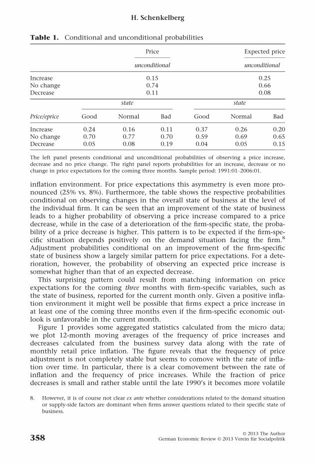
inflation environment. For price expectations this asymmetry is even more pro-nounced (25% vs. 8%). Furthermore, the table shows the respective probabilitiesconditional on observing changes in the overall state of business at the level ofthe individual firm. It can be seen that an improvement of the state of businessleads to a higher probability of observing a price increase compared to a pricedecrease, while in the case of a deterioration of the firm-specific state, the proba-bility of a price decrease is higher. This pattern is to be expected if the firm-spe-cific situation depends positively on the demand situation facing the firm.8

Adjustment probabilities conditional on an improvement of the firm-specificstate of business show a largely similar pattern for price expectations. For a dete-rioration, however, the probability of observing an expected price increase issomewhat higher than that of an expected decrease.

This surprising pattern could result from matching information on priceexpectations for the coming three months with firm-specific variables, such asthe state of business, reported for the current month only. Given a positive infla-tion environment it might well be possible that firms expect a price increase inat least one of the coming three months even if the firm-specific economic out-look is unfavorable in the current month.

Figure 1 provides some aggregated statistics calculated from the micro data;we plot 12-month moving averages of the frequency of price increases anddecreases calculated from the business survey data along with the rate ofmonthly retail price inflation. The figure reveals that the frequency of priceadjustment is not completely stable but seems to comove with the rate of infla-tion over time. In particular, there is a clear comovement between the rate ofinflation and the frequency of price increases. While the fraction of pricedecreases is small and rather stable until the late 1990’s it becomes more volatile

Table 1. Conditional and unconditional probabilities

Price Expected price

unconditional unconditional

Increase 0.15 0.25No change 0.74 0.66Decrease 0.11 0.08

state state

Price/eprice Good Normal Bad Good Normal Bad

Increase 0.24 0.16 0.11 0.37 0.26 0.20No change 0.70 0.77 0.70 0.59 0.69 0.65Decrease 0.05 0.08 0.19 0.04 0.05 0.15

The left panel presents conditional and unconditional probabilities of observing a price increase,decrease and no price change. The right panel reports probabilities for an increase, decrease or nochange in price expectations for the coming three months. Sample period: 1991:01–2006:01.

8. However, it is of course not clear ex ante whether considerations related to the demand situationor supply-side factors are dominant when firms answer questions related to their specific state ofbusiness.

H. Schenkelberg


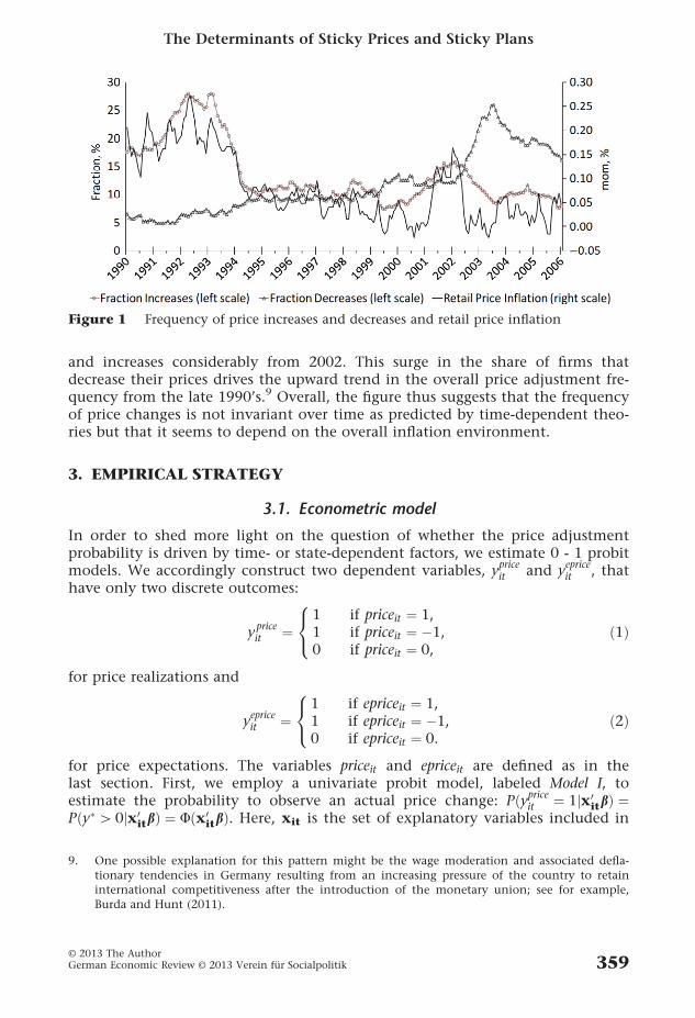
and increases considerably from 2002. This surge in the share of firms thatdecrease their prices drives the upward trend in the overall price adjustment fre-quency from the late 1990’s.9 Overall, the figure thus suggests that the frequencyof price changes is not invariant over time as predicted by time-dependent theo-ries but that it seems to depend on the overall inflation environment.

3. EMPIRICAL STRATEGY

3.1. Econometric model

In order to shed more light on the question of whether the price adjustmentprobability is driven by time- or state-dependent factors, we estimate 0 - 1 probitmodels. We accordingly construct two dependent variables, y

priceit and y

epriceit , that

have only two discrete outcomes:

ypriceit ¼

1 if priceit ¼ 1,1 if priceit ¼ �1,0 if priceit ¼ 0,

8<: ð1Þ

for price realizations and

yepriceit ¼

1 if epriceit ¼ 1,1 if epriceit ¼ �1,0 if epriceit ¼ 0.

8<: ð2Þ

for price expectations. The variables priceit and epriceit are defined as in thelast section. First, we employ a univariate probit model, labeled Model I, toestimate the probability to observe an actual price change: Pðypriceit ¼ 1jx0

itbÞ ¼Pðy� [0jx0

itbÞ ¼ Uðx0itbÞ. Here, xit is the set of explanatory variables included in

Figure 1 Frequency of price increases and decreases and retail price inflation

9. One possible explanation for this pattern might be the wage moderation and associated defla-tionary tendencies in Germany resulting from an increasing pressure of the country to retaininternational competitiveness after the introduction of the monetary union; see for example,Burda and Hunt (2011).



the model and y�it denotes the latent price variable assumed to underly the datagenerating process: y�it ¼ x0

itbþ uit . Second, in order to analyze the pricing planadjustment probability, a bivariate probit model, labeled Model II, is estimated tocontrol for a possible correlation between the price setting decision and theupdating of pricing plans leading to a more efficient estimation compared to asimple univariate specification (Cameron and Trivedi, 2007). The probabilitymodel can be derived from the following latent variable specification:

y�1it ¼ x01itb1 þ �1it

y�2it ¼ x02itb2 þ �2it ;

ð3Þ

where y�1it and y�2it denote the latent variables underlying the observed dependentvariables y

priceit and y

epriceit , respectively, and b1 and b2 are vectors of unknown

parameters. �1i and �2i are error terms that are assumed to be distributed as bivari-ate standard normal with correlation q.10

Hence, we estimate simple change/no change probit models as a first stepinstead of more explicitly exploiting the ordinal structure of the dependent vari-ables estimating, for instance, a multinomial probit model. Our approach canthus be interpreted as a ‘test’ for state-dependence; if the coefficients of all statevariables are insignificant, price setting is time-dependent. If, however, the coeffi-cients of all the time-dependent variables are insignificant, price setting can beconsidered state-dependent. In case factors from both sets of explanatory vari-ables are significant there are two types of price changes; however, in this case atleast a significant portion of the prices included in the sample are changedaccording to state-dependent rules.

As a further investigation it is, however, instructing to analyze the drivers ofprice increases and decreases separately. This exercise is not meant as a direct testfor state-dependence, but may rather provide some additional insights concern-ing the behavioral parameters underlying the price adjustment decision. We thusconstruct four further binary dependent variables: yincrit , ydecrit , ye incr

it and ye decrit

indicating a price increase and decrease as well as an expected price increase anddecrease, respectively. First, we estimate univariate probit models with yincrit andydecrit as dependent variables, denoted as Model III and Model IV, respectively. Sec-ond, to additionally investigate potential asymmetries in the updating of pricingplans, we estimate bivariate probit models according to equation (3) above. Inthis case, y�1it and y�2it refer to the dependent variables denoting (expected) priceincreases and (expected) price decreases, respectively (Model V and Model VI).11

All models are estimated without the explicit inclusion of individual-specificeffects. First, to account for observable heterogeneity, sector-specific dummy vari-ables are included in the set of regressors. Moreover, due to the firm-specificnature of the dataset at hand, arguably, a large extent of firm heterogeneity is

10. In order to identify the parameters of the model given in equation (3), we normalize the coeffi-cient of one of the time-dependent variables in the vector x0

1it, Taylor6it , to one. Our results arerobust to varying the exclusion restriction.

11. As an alternative approach, one could exploit the ordinal structure of the data and estimateordered probit models. However, an ordered probability specification may conceal potentialasymmetries between price increases and decreases and is therefore not chosen as benchmarkmodel. Our main conclusions are, however, unchanged if we estimate ordered probit modelsinstead; please refer to the results presented in the supplementary material.

H. Schenkelberg


already captured by some of the regressors (Lein, 2010). To mitigate the remain-ing problem of unobserved heterogeneity, we employ the Mundlak–Chamberlainapproach of correlated random effects assuming the individual-specific effects tobe related to observed characteristics in the model. Relative to fixed effects mod-els, such as the conditional logit model, this specification permits consistent esti-mation of all parameters, including coefficients of time-invariant covariates, suchas sectoral dummies. Furthermore, a random effects specification is appropriatefor the application at hand since we analyze a sample of price changes that aretaken randomly from the population of all prices changes in the economy.12

To implement this approach for our model, we add a vector of firm-specifictime averages of the individual-specific variables to the set of regressors, whichyields consistent estimates also in the case of pooled estimation (Mundlak,1978). In effect, we assume the latent variable specification to take on the follow-ing form: y�it ¼ x0

itbþ �x0iaþ uit , where �x0

ia indicate the firm-specific time averagesof the regressors.13 Finally, because of the occurrence of multi-product firms inthe sample, standard errors are clustered by firm in order to control for potentialcorrelations between observation-units.

3.2. Explanatory variables

For all the six models explained above, two specifications are estimated. In speci-fication (1) it will be analyzed whether, next to time dependent variables, mea-sures reflecting the state of the firm as well as macroeconomic and institutionalfactors have a significant effect on the probability of price adjustment. First, weinclude the variable reflecting the overall state of business described in the previ-ous section; stateit . Because of potential asymmetries in the effects of an improve-ment and a deterioration in the individual state, two corresponding dummiesare constructed of this variable, denoted state� and stateþ for deteriorations andimprovements, respectively. We do not consider other firm-specific variablesincluded in the dataset because of potential endogeneity concerns, particularlywith regard to the questions on business expectations. In addition, the variablesreflecting the overall state of business are likely to sufficiently capture the overallbusiness situation of the individual firm since they implicitly include informa-tion on all factors relevant to the firm-specific state of business such as the reve-nue and profit situation or the competitive environment as well as labor marketdevelopments. Importantly, endogeneity is unlikely to be an issue with regard tothese measures because firms are explicitly asked to consider the latest tendencieswith regard to the state of business when answering this question. Hence, firmsare asked explicitly to take into account past developments rather than expecta-tions concerning the future when answering this question. Therefore, the per-ceived state of business reported by the firms in each month is arguably notseverely affected by the current pricing decision. Furthermore, any remaining

12. See, for instance, Rumler et al. (2011) for another application of the random effects model in asimilar setting.

13. Our results are robust if we estimate the model using a correlated random effects panel probitspecification. Furthermore, our main findings do not change if we exclude the time averages.Detailed results can be found in the supplementary material.



endogeneity concerns with respect to this variable are largely mitigated sinceresults are robust to including both variables in first lags as well as to usinginstrumental variables estimation.14 See the supplementary material, availableupon request, for more details.

Moreover, we include aggregate variables to capture the macroeconomic andinstitutional environment facing the firms. Arguably, the most important macro-economic variable for price setting at the retail level is the overall rate of infla-tion. According to, for instance, Dotsey et al. (1999), an increase in inflationleads to a decline in relative prices of individual firms which should increase theprobability of repricing. Thus, the sectoral rates of inflation are included asregressors. The importance of sectoral inflation for price setting is well estab-lished in the literature; in fact, the effect of this variable can be interpreted as anindicator of the transmission of price shocks between firms.15 In standard menucost models, the likelihood of price adjustment depends on the distance of theactual to the optimal price, which itself varies with the state of the economy;this distance thus depends on changes in macroeconomic factors, accumulatedsince the last price change. For instance, in the target threshold model of Cecch-etti (1986), the probability of a price change depends on the difference betweenthe optimal price the firm had set if there were no costs of price adjustment andthe actual price set by the firm. If this difference exceeds a certain threshold, theprice will be adjusted because keeping the actual price would then be more costlythan the price adjustment. Hence, according to this model, firms wait with thenext price adjustment until the accumulated change in the rate of inflation islarge enough. In order to capture the idea of this target-threshold model, thecumulative rate of sectoral inflation is the relevant variable to include in themodel instead of the monthly or quarterly rate of inflation.16 However, we havechecked that our results are robust to the inclusion of the quarterly rate of infla-tion; please refer to the supplementary material and Section 4 for more details.

14. In particular, we additionally estimate a linear model in order to be able to perform a two-stageleast square instrumental variables estimation. For this model, we assume the variables state�

and stateþ to be endogenous regressors. As instruments we consider first lags of these two vari-ables. For the application at hand, it is difficult to find alternative instruments, which reflectthe individual-specific state. Using one of the other firm-specific variables in the dataset is notan option, because these measures are even more likely lead to reverse causality.

15. Arguably, including the rate of inflation only may not cover the entire macroeconomic envi-ronment facing the firms. To still control for additional factors that potentially affect price set-ting in retail, we estimate the models additionally including a set of time dummies, that is,time-fixed effects, instead of the aggregate and institutional variables, which are intended tocapture all shocks that equally affect all firms in a given month. As shown in the supplemen-tary material, our main results are not affected by this variation. Furthermore we have checkedthat our results are robust to including year dummies instead of the time-fixed effects and theaggregate and institutional variables.

16. Card and Sullivan (1988) show that cumulative variables may lead to endogeneity issues andthus to biased estimators because they can be expressed as xit ¼ 1þ ð1� yit�1Þxit�1. Thus, toaccount for possible endogeneity problems associated with the cumulative inflation variable themodel is estimated by including the first individual observation of the dependent variable as anadditional regressor, as has been suggested by Wooldridge (2005) and applied by Loupias andSevestre (2010). Furthermore, our results are robust to including month-on-month changes inthe sectoral price indices instead of cumulative changes.

H. Schenkelberg


Next to the sectoral rates of inflation a set of dummy variables controlling forimportant institutional events is added. In particular, we consider the introduc-tion of the Euro as well as changes in the VAT rate as relevant institutionalchanges.

We furthermore add a set of time-dependent variables to specification (1). Toinvestigate whether firms in the dataset employ Taylor-type pricing, Taylor dum-mies are constructed indicating that the last price change occurred a fixed periodago. Furthermore, seasonal dummies are constructed to examine whether theprobability of repricing according to fixed time intervals is increased.17 Finally,we include sector-specific dummy variables. In order to shed more light on theimportance of input costs, variables indicating the frequency of input pricechanges are included in an augmented model, labeled specification (2).18 Bothwholesale and manufacturing price developments are considered, because retailfirms use products of both sectors as inputs. Please refer to the supplementarymaterial for more details on the construction of the explanatory variables.

4. RESULTS

4.1. Time- vs. state-dependence

As a first step, we want to investigate whether, relative to time-dependent vari-ables, state-dependent factors are important for the probability to observe a pricechange. We first estimate a simple change/no change probit model with the bin-ary variable y

priceit as dependent variable, labeled Model I. Results for the baseline

price setting equation (1) and the specification including intermediate inputcosts (2) for price changes are shown in the second and third column of Table 2.The table reports marginal effects for outcome 1 (price change) as well as stan-dard errors, clustered by firm. First, in specification (1) most time-dependent vari-ables have significant effects on the probability of price adjustment.

For instance, for a firm that changed its price exactly four quarters ago, theprice change adjustment probability is raised by 23.5 percentage points in agiven period. Moreover, Wald tests indicate that the Taylor dummies are jointlysignificant. Furthermore, seasonality seems to be present in price setting at theretail level; compared to the baseline season spring, price changes are more likelyin winter and less likely in fall.

Next to the time-dependent variables, the firm-specific measures show highlysignificant effects and have the expected signs. The table shows that an impair-ment in the state of business increases the chance to observe a price change by

17. Arguably, if seasonality is important for price setting, prices may be changed at fixed points oftime. We have checked that our results are insensitive to the inclusion of specific month dum-mies (e.g. dummies for January, April, July and October). However, since it is not clear a prioriin which particular month firms tend to change their prices, we stick with the inclusion of sea-sonal dummies in the benchmark model.

18. In principle, specification (1) may be estimated on a larger sample compared to model (2),where firm-products that could not be assigned a corresponding wholesale measure droppedout. However, both specifications are estimated on the same reduced sample in order to be ableto compare the respective results. We have checked that results are insensitive to extending thesample for specification (1).



Table

2.

Thedeterminants

ofprice

changes

andpricingplanadjustmen

ts

Model

I:probit

estimatesdep

enden

t:yprice

Model

II:bivariate

probit

estimatesdep

enden

t:yprice,

ye

price

(1)

(2)

(1)

(2)

ME

SEME

SEME

SEME

SE

State

�0.021�

0.006

0.030��

0.012

0.004

0.004

0.011

0.015

State

þ0.073��

�0.008

0.068��

�0.017

0.076��

�0.007

0.071��

�0.017

Inflation

0.059��

�0.006

0.050��

�0.009

0.052��

�0.006

0.044��

�0.006

EUR

0.061��

�0.012

0.080��

�0.023

0.061��

�0.018

0.079��

�0.018

VAT

0.045��

�0.008

0.061��

�0.017

0.057��

�0.014

0.072��

�0.014

Price_w

s0.076��

�0.023

0.081��

�0.023

Price_m

0.141��

�0.020

0.123��

�0.018

Taylor6

0.194��

�0.005

0.191��

�0.013

0.164��

�0.012

0.161��

�0.011

Taylor12

0.235��

�0.005

0.236��

�0.011

0.188��

�0.010

0.188��

�0.010

Taylor18

0.045��

�0.006

0.056��

�0.012

0.040��

�0.012

0.051��

�0.011

Taylor24

0.133��

�0.006

0.141��

�0.012

0.101��

�0.011

0.108��

�0.011

Winter

0.084��

�0.007

0.070��

�0.012

0.033��

�0.011

0.018

0.011

Summer

0.005

0.007

0.020�

0.011

�0.011

0.009

0.002

0.009

Fall

�0:023��

�0.007

0.001

0.015

0.031��

�0.012

0.051��

�0.012

Log-Lik.

�27304.015

�27132.108

�55131.787

�54882.677

Obs.

46611

46611

46611

46611

Wald

test

forjointsignificance

ofTaylordummies

Chi2

636.585

460.720

2417.620

2417.100

Prob>ch

i20.000

0.000

0.000

0.000

�� p<0.01,��p\0:05,� p\0:1.Thetable

reportsmarginaleffects(M

E)androbust

standarderrors

(SE.),clustered

byfirm

.MEsare

calculatedforoutcomes

‘price

change’

and‘price

changeandex

pectedprice

change’,resp

ectively,settingallvariablesatth

eirmea

n.Forbinary

regressors,th

eeffect

isfordis-

cretech

angefrom

0to

1.W

eadditionallyincludebutdonotreport

firm

-specificaverages

ofth

eindividual-sp

ecificvariablesandsectoraldummies.

H. Schenkelberg


2.1 percentage points while improvements in the firm-specific condition raisethe repricing probability by 7.3 percentage points on average.

Table 2 furthermore shows that the factors capturing the aggregate environ-ment of the firms are important next to the idiosyncratic factors. The effect ofcumulative changes of the sectoral rate of inflation is highly significant and eco-nomically important; a marginal change in this variable increases the pricechange probability by 5.9 percentage points. This result is in line with the target-threshold model by Cecchetti (1986) and the idea that firms tend to changeprices once accumulated aggregate shocks and thus the difference between theoptimal and the actual price are large enough. As indicated above, we havechecked robustness of the results when including the quarterly instead of thecumulative rate of inflation, that is, the rate of inflation between timet�3 andtimet . As shown in the supplementary material, the results are insensitive to thisalteration; the quarterly rate of inflation is an important determinant of the tim-ing of price adjustment, too.19

Additionally, the table shows that changes in the institutional environmentsignificantly affect the timing of price adjustment; the introduction of the Euroled to a price adjustment probability that is increased by 6.1 percentage points,while an increase in the VAT rate has a positive effect of around 4.5 percentagepoints.

Column three of Table 2 shows regression results of specification (2) includingchanges in intermediate input costs for Model I. Both measures are highly signifi-cant and have the expected effects. A marginal change in the measure of manu-facturing price changes increases the likelihood of a price change by 14.1percentage points, while the marginal effect of the sector-specific measure of thewholesale price adjustment frequency is around 7.6 percentage points. This pro-vides evidence in favor of cost-based pricing, which is in line with resultsreported by Fabiani et al. (2006) for the Euro area and Eichenbaum et al. (2011)for the United States. Moreover, these results show that apparently, there is notmuch stickiness at the last stage of processing; retail firms immediately respondto changes in intermediate input prices. This is in line with theoretical modelsthat integrate an explicit production structure in a pricing framework as Basu(1995) and, more recently, Nakamura and Steinsson (2010).

4.2. Assessing sticky plan models

In order to shed more light on the plausibility of state-dependent sticky planmodels, specifications (1) and (2) are additionally estimated using a bivariate pro-bit model, labeled Model II, which controls for a possible correlation betweenthe processes underlying price adjustment and the updating of pricing plans.Results from a Wald test performed to test the independence of equationshypothesis (q=0) indicates that a bivariate specification leads to a more efficient

19. Additionally, results are insensitive if the rate of inflation between timet�4 and timet or betweentimet�6 and timet is included instead; these results are available upon request. However, a vari-able reflecting month-on-month changes in the rate of inflation is insignificant, which in factfurther confirms that firms do not consider monthly changes in the aggregate economic envi-ronment for their price adjustment decision but wait until aggregate shocks are large enough.Again, this is in line with the target-threshold model of Cecchetti (1986).



estimation. Regression results are reported in columns four and five of Table 2above. The table shows marginal effects of the regressors for outcome possibility(1,1): price change and expected price change.

Overall, the explanatory variables show quite similar effects on the probabilityof both a change in price plans and an actual price adjustment. As for Model I,also time-dependent factors seem to play a role for the updating of pricing plans;the Taylor dummies and most seasonal dummies have significant effects in speci-fication (1). Moreover, changes in the institutional environment and cumulativechanges in the sectoral rate of inflation are significant and have the expected sign;marginal effects are similar in order of magnitude as compared to the results forModel I. With respect to the variables reflecting the state of business of the indi-vidual firm, Table 2 shows that improvements in the firm-specific condition leadto a higher chance to observe both a price change and a pricing plan adjustmentof 7.6 percentage points. However, deteriorations do not seem to be significantlyrelated to the joint probability of a price change and an expected price change.

Results from specification (2) show that intermediate input price changes aresignificantly related to the chance to observe both a price change and a pricingplan adjustment. Moreover, the economic effects of these variables on the jointprobability are similar compared to the effects on the price change probabilityonly. While the results for most of the state-dependent variables and Taylordummies are robust to the inclusion of these variables, interestingly, the seasonaldummies appear to be somewhat sensitive to the econometric specification esti-mated. This suggests that seasonality observed after estimating specification (1)might in fact not be due to time-dependent pricing behavior alone, at least withregard to expected price adjustment in winter as compared to the benchmarkseason spring.

It should be noted at this point that estimating a simple univariate probitmodel with ye price as dependent variable leads to very similar results. First, thisindicates that our main conclusions are not sensitive to the model used and sec-ond, it confirms that a significant portion of retail firms seems to adjust theirpricing plans according to a state-dependent pattern, too.

4.3. Pricing decisions across different inflation regimes

Two tentative conclusions can be drawn from the results given above. First, indi-cated by the relatively large effects of the Taylor dummies, time-dependent fac-tors seem to be important for price setting at the retail level. Second, however,the finding that the firm-specific variables, aggregate factors and intermediateinput prices show statistically and economically significant effects implies that anon-negligible portion of the firms in the sample adjust their prices according toaggregate and idiosyncratic states.

Given the very low overall rate of inflation in Germany during the time periodconsidered, the finding that state-dependence seem to play an important role isquite remarkable. It is often assumed in theoretical models of price setting thattime-dependent pricing assumptions may be appropriate during periods of lowand not so volatile inflation;20 our empirical evidence suggests, however, that

20. See, for instance, the heterogeneous sticky price model by Carvalho (2006).

H. Schenkelberg


this may in fact not be the case. To further investigate differences in price settingacross different inflation regimes, we split the sample and additionally estimatedModels I and II separately for two different sample periods. The first period is1991:01–1996:12, where the annual rate of CPI inflation averages to around3.3%, and the second period investigated is 1997:01–2006:01 where inflationwas brought down even further to around 1.4%, on average. Correspondingregression results, which can be found in the supplementary material, show thatoverall, the behavioral parameters are robust across the two sample periods.State-dependence seem to matter for price setting during both periods; mostfirm-specific variables, changes in the VAT rate and changes in the wholesaleprice measure significantly affect the decision both to change prices and toupdate pricing plans. Important exceptions are the sectoral rate of inflation and,for the joint probability to observe both a change in the actual price and thepricing plan, changes in the manufacturing price measure; these variables are sig-nificant in the first period, but do not have significant effects in second period.Given the very low rate of inflation and accompanying low inflation variabilitythis is of course not surprising. However, the finding that most of the otherstate-dependent factors insensitively affect pricing across inflation regimes clearlyimplies that time-dependence does not seem to be a good approximation to theprice adjustment mechanism, even in periods of exceptionally low inflation.

4.4. The Determinants of Price Increases versus Price Decreases

Next to analyzing the price change and pricing plan adjustment probabilities, itis also interesting to investigate the determinants of (expected) price increasesand decreases separately, labeled Model III and Model IV. Such an analysis mayshed more light on the patterns underlying variations in the extensive margin ofprice adjustment observed in the data and may reveal potential asymmetries inprice setting. For instance, Peltzman (2000) shows that the reaction of priceincreases to positive cost shocks is substantially stronger than the response ofprice decreases to negative cost changes in the United States. Similarly, reportingevidence from a one-time Euro-area interview study, Fabiani et al. (2006) indicatethat cost changes of raw material are among the most important factors leadingto positive price changes, while the factors underlying price decreases are not asclearly classifiable as relating to the demand or cost situation. In order to shedmore light on these issues, we first estimate specifications (1) and (2) with yincr

and ydecr as dependent variable, respectively; the corresponding marginal effectsand clustered standard errors are shown in Table 3. Furthermore, the specifica-tions are estimated using bivariate probit models (Models V and VI) with yincr

and ye incr as well as ydecr and ye decr as dependent variables, respectively. Theseresults are displayed in Table 4. Both tables show that first, Taylor dummies areimportant for changes in both (expected) price increases and decreases; Waldtests indicate that these variables are jointly significant. However, while seasonal-ity seems to be somewhat important for realized price increases, these effects arenot found for price decreases.

With respect to the state-dependent variables, Table 3 shows that while,overall, most of these factors significantly influence the timing of bothprice increases and decreases, there are some differences in the effects of some



Table

3.

Thedeterminants

ofprice

increa

sesanddecreases

Model

III:probit

estimatesdep

enden

t:yincr

Model

IV:probit

estimatesdep

enden

t:ydecr

(1)

(2)

(1)

(2)

ME

SEME

SEME

SEME

SE

State

��0

:051��

�0.010

�0:036��

�0.010

0.073��

�0.009

0.066��

�0.009

State

þ0.053��

0.020

0.037�

0.017

0.015

0.019

0.024

0.018

Inflation

0.042��

�0.006

0.031��

�0.006

0.005

0.006

0.009

0.006

EUR

0.043��

0.022

0.068��

�0.024

0.021

0.017

0.016

0.017

VAT

0.092��

0.016

0.101��

�0.017

�0:042��

�0.009

�0:036��

�0.009

Price_w

s0.333��

�0.030

�0:223��

�0.024

Price_m

0.112��

�0.019

�0.004

0.013

Taylor6

0.090��

�0.011

0.083��

�0.010

0.091��

�0.009

0.091��

�0.009

Taylor12

0.131��

�0.010

0.128��

�0.010

0.086��

�0.009

0.088��

�0.009

Taylor18

�0:032��

�0.011

�0:013��

�0.011

0.064��

�0.008

0.055��

�0.008

Taylor24

0.036��

�0.010

0.050��

�0.010

0.079��

�0.008

0.073��

�0.009

Winter

0.081��

�0.012

0.041��

�0.012

�0.002

0.009

0.019�

0.010

Summer

0.011

0.012

0.024�

0.011

0.001

0.008

0.002

0.008

Fall

�0:025��

0.010

0.000

0.010

0.002

0.010

�0.004

0.011

Log-Lik.

�23020.529

�21956.936

�18471.771

�17853.769

Obs.

46611

46611

46611

46611

Wald

test


ofTaylordummies

Chi2

181.560

175.670

156.460

152.080

Prob>ch

i20.000

0.000

0.000

0.000

�� p\0:01,��p\0:05,� p\0:1.Thetable


E)androbust

standarderrors

(St.Err.),clustered

byfirm

.MEsare

calculatedforout-

comes

‘price

increa

se’and‘price

decrease’,resp


eirmea

n.Forbinary

regressors,th

eeffect

isfordiscretech

angefrom

0to

1.W

eadditionallyincludebutdon’treport

firm

-specificaverag

esofth

eindividual-sp

ecificvariablesandsectoraldummies.

H. Schenkelberg


Table

4.

Thedeterminants

ofex

pectedprice

increa

sesanddecreases

Model

V:bivariate

probit

estimatesdep

enden

t:yincr,

ye

incr

Model

VI:

bivariate

probit

estimatesdep

enden

t:ydecr ,

ye

decr

(1)

(2)

(1)

(2)

ME

SEME

SEME

SEME

SE

State

��0

:040��

�0.009

�0:030��

�0.009

0.028��

�0.005

0.025��

�0.005

State

þ0.029�

0.016

0.019

0.013

0.020��

�0.007

0.022��

�0.007

Inflation

0.030��

�0.004

0.021��

�0.004

0.002

0.002

0.004

0.003

EUR

\0.023��

0.014

0.041��

�0.016

0.015�

0.007

0.012

0.009

VAT

0.077��

�0.012

0.085��

�0.012

�0:016��

�0.004

�0:014��

�0.003

Price_w

s0.208��

0.023

�0:071��

�0.011

Price_m

0.087��

0.014

�0.006

0.005

Taylor6

0.065��

�0.009

0.059��

�0.008

0.030��

�0.005

0.029��

�0.005

Taylor12

0.091��

�0.009

0.086��

�0.009

0.024��

�0.004

0.023��

�0.004

Taylor18

�0:015��

�0.007

�0.002

0.007

0.023��

�0.005

0.019��

�0.004

Taylor24

0.026��

�0.007

0.036��

�0.007

0.023��

�0.004

0.020��

�0.004

Winter

0.063��

�0.008

0.034��

�0.007

�0:021��

�0.004

�0:014��

�0.004

Summer

0.033��

�0.009

0.042��

�0.008

�0:026��

�0.004

�0:024��

�0.004

Fall

0.014

0.007

0.033��

�0.007

0.001

0.003

�0.002

0.003

Log-Lik.

�47745.614

�46466.383

�33056.303

�32340.609

Obs.

46611

46611

46611

46611

Waldtest


ofTaylordummies

Chi2

1639.600

1508.890

2195.680

2211.890

Prob>ch

i20.000

0.000

0.000

0.000

�� p\0:01,

��p\0:05,

� p\0:1.Thetable


E)and

robust

standard

errors

(SE),

clustered

byfirm

.MEsare

calculated

forout-

comes

‘price

increa

seandex

pectedprice

increa

se’and‘price

decrease

andex

pectedprice

decrease,’resp


eirmea

n.For

binary

regressors,th

eeffect

isfordiscretech

angefrom

0to

1.W

eadditionallyincludebutdon’t

report

firm

-specificaverag

esofth

eindividual-sp

ecific

variab

lesandsectoraldummies.



particular regressors. First, while changes in the sectoral rates of inflation as wellas the introduction of the Euro have significant effects on the decision to raiseprices, these variables do not appear to significantly change the likelihood ofobserving a price decrease. A similar pattern can be observed for the joint proba-bility of price increases (decreases) and expected price increases (decreases), ascan be seen in Table 4. Since we analyze pricing during a positive inflation envi-ronment, the finding that the price decrease probability does not significantlyreact to changes in inflation is, however, not too surprising.

Furthermore, with regard to intermediate input cost changes, our results showthat while such cost changes have an important effect on the chance to observe aprice increase with marginal effects amounting to 0.33 and 0.11 for wholesale andmanufacturing price changes, respectively, the effects on the price decrease proba-bility are much smaller (see Table 3). For changes in the wholesale price measurethe marginal effect is 0.22, while the price decrease probability is not significantlyaffected by changes in manufacturing prices. These findings confirm the US. evi-dence reported by Peltzman (2000) as well as the results of the one-time Euro areainterview study conducted by Fabiani et al. (2006) that cost shocks can haveasymmetric effects on price increases and decreases, respectively. In addition,Table 4 shows that these results also hold for the joint probability of observingboth a price increase (decrease) and an expected price increase (decrease).

Furthermore, with respect to the two variables indicating the specific state ofthe firm, there are some asymmetries in the response of price increases anddecreases, respectively. While the effect of a deterioration in the state of businessis, as expected, negative (positive) for price increases (decreases) with marginaleffects of �0.036 and 0.066, respectively, for specification (2), the effect of animprovement of the firm-specific condition is not significant for price decreases.

The regression results shown in columns 8 and 9 of Table 4 indicate that bothan improvement and a deterioration in the state of business has a significantlypositive effect on the joint probability of observing both a price decrease and anexpected price decrease, which seems somewhat puzzling. Since, as can be seen inTable 3, improvements in the state of business are not important for the probabil-ity to observe a price decrease, this surprising pattern may be driven by the effectsof this variable on the decision to adjust the pricing plan, that is, to decrease pricesin the future. Hence, this result suggests that on average, firms expect to decreasetheir prices in the future if the current business outlook is favorable. This seem-ingly surprising finding may be reconciled by noting that improvements in thestate of business may also be due to improvements in the cost situation faced bythe firms. If the cost situation is currently favorable, firms may want to decreaseprices in the future if it turns out that costs can be kept low for several periods.This may suggest that while, in line with Peltzman (2000), negative cost shocksare not as important for the decision to decrease prices, a currently favorable costenvironment may well affect the decision to decrease prices in the future.

5. CONCLUSION

This study contributes to the empirical literature on price stickiness by analyzingthe patterns underlying the price setting and pricing plan adjustment behavior

H. Schenkelberg


of German retail firms using a new firm-level business survey dataset. First,regressing the price adjustment probability not only on time-dependent andmacroeconomic variables but also on factors characterizing the individual-spe-cific condition of firms, we find that next to time-dependent variables such as,most notably, Taylor dummies, most state-dependent factors significantly changethe repricing probability. Cumulative changes in the sectoral rate of inflation aswell as the introduction of the Euro or changes in the VAT rate determine thetiming of price adjustment; price setting thus seems to respond to economicshocks. Moreover, the variables describing the specific state of the firm turn outto be highly significant. Hence, a significant portion of prices are changedaccording to state-dependent rules. This suggests that standard time-dependentmodels �a la Calvo (1983) or Taylor (1980) may not be sufficient to describe theprice adjustment process – even for a period of low inflation. With respect to theimportance of intermediate input cost variables, regression results show thatinput price variability is indeed an important determinant of price adjustmentand that retail firms immediately respond to input cost changes. Explicitly mod-eling the transmission of price changes through the chain of production is thusa valid approach. Second, we find that changes in price expectations are drivenby similar factors as changes in actual prices. Most of the firm-specific variables,macroeconomic measures as well as institutional dummies are highly significantand economically important. These results are in line with state-dependent pric-ing plan models of, for instance, Burstein (2006). Finally, we separately analyzethe factors driving prices upwards and downwards, respectively, in order toinvestigate if there are asymmetries in the response of prices to certain shocks atthe firm-level. Our results indicate that price increases respond stronger to costshocks than price decreases, which is in line with existing US evidence.

ACKNOWLEDGEMENTS

I would like to thank, without implicating, two anonymous referees, managingeditor Christoph Schmidt, Kai Carstensen, Daniel Dias, Heinz Herrmann, JohannesHoffmann, Gerhard Illing, Ulf von Kalckreuth, Harald Stahl and seminar partici-pants at Deutsche Bundesbank and LMU Munich as well as participants at the 2011European Meeting of the Econometric Society in Oslo, the 2011 Spring Meeting ofYoung Economists at University of Groningen and several other conferences andworkshops for helpful comments. Financial support from the German ResearchFoundation through GRK 801 is gratefully acknowledged. All errors are my own.

Address for correspondence: Heike Schenkelberg, Munich Graduate School ofEconomics, Kaulbachstrasse 45 80539 Munich, Germany. Tel: +49 89 2180 5629;e-mail: [email protected]

REFERENCES

Alvarez, F. E., F. Lippi, and L. Paciello, (2010), ‘Optimal Price Setting with Observationand Menu costs’, NBER Working Papers 15852, National Bureau of Economic Research,Inc.



Alvarez, L. J., E. Dhyne, M. Hoeberichts, C. Kwapil, H. L. Bihan, P. Lnnemann, F. Martins,R. Sabbatini, H. Stahl, P. Vermeulen, and J. Vilmunen, (2006), ‘Sticky prices in the euroarea: A summary of new micro-evidence’, Journal of the European Economic Association 4,575–584.

Aucremanne, L. and E. Dhyne, (2005), ‘Time-dependent Versus State-dependent Pricing –A Panel Data Approach to the Determinants of Belgian Consumer Price Changes’,Working Paper Series 462, European Central Bank.

Basu, S. (1995), ‘Intermediate goods and business cycles: Implications for productivity andwelfare’, American Economic Review 85, 512–531.

Becker, S. O. and K. Wohlrabe, (2008), ‘Micro data at the ifo institute for economicresearch – the “ifo business survey”, usage and access’, Journal of Applied Social Sciences128, 307–319.

Bils, M. and P. J. Klenow, (2004), ‘Some evidence on the importance of sticky prices’,Journal of Political Economy 112, 947–985.

Blinder, A. S. (1991), ‘Why are prices sticky? preliminary results from an interview study’,American Economic Review 81, 89–96.

Bonomo, M. and C. Carvalho, (2004), ‘Endogenous time-dependent rules and inflationinertia’, Journal of Money, Credit and Banking 36, 1015–1041.

Burda, M. C. and J. Hunt, (2011), ‘What Explains the German Labor Market Miracle in theGreat Recession?’, NBER Working Papers 17187, National Bureau of Economic Research,Inc.

Burstein, A. T. (2006), ‘Inflation and output dynamics with state-dependent pricing deci-sions’, Journal of Monetary Economics 53, 1235–1257.

Calvo, G. A. (1983), ‘Staggered prices in a utility-maximizing framework’, Journal of Mone-tary Economics 12, 383–398.

Cameron, A. C. and P. K. Trivedi, (2007), Microeconometrics: Methods and Applications, Cam-bridge University Press, New York.

Card, D. and D. G. Sullivan, (1988), ‘Measuring the effect of subsidized training programson movements in and out of employment’, Econometrica 56, 497–530.

Carvalho, C. (2006), ‘Heterogeneity in price stickiness and the real effects of monetaryshocks’, B.E. Journal of Macroeconomics 6, 1.

Cecchetti, S. G. (1986), ‘The frequency of price adjustment: A study of the newsstandprices of magazines’, Journal of Econometrics 31, 255–274.

Dhyne, E., L. J. Alvarez, H. L. Bihan, G. Veronese, D. Dias, J. Hoffmann, N. Jonker,P. Lunnemann, F. Rumler, and J. Vilmunen, (2006), ‘Price changes in the euro area andthe united states: Some facts from individual consumer price data’, Journal of EconomicPerspectives 20, 171–192.

Dotsey, M., R. G. King, and A. L. Wolman, (1999), ‘State-dependent pricing and the gen-eral equilibrium dynamics of money and output’, Quarterly Journal of Economics 114,655–690.

Eichenbaum, M., N. Jaimovich, and S. Rebelo, (2011), ‘Reference prices, costs, and nomi-nal rigidities’, American Economic Review 101, 234–62.

Fabiani, S., M. Druant, I. Hernando, C. Kwapil, B. Landau, C. Loupias, F. Martins, T.Math, R. Sabbatini, H. Stahl, and A. Stokman, (2006), ‘What firms’ surveys tell usabout price-setting behavior in the euro area’, International Journal of Central Banking2, 3–47.

Gertler, M. and J. Leahy, (2008), ‘A phillips curve with an ss foundation’, Journal of Politi-cal Economy 116, 533–572.

Golosov, M. and R. E. Lucas, (2007), ‘Menu costs and phillips curves’, Journal of PoliticalEconomy 115, 171–199.

Huang, K. X. D. and Z. Liu, (2001), ‘Production chains and general equilibrium aggregatedynamics’, Journal of Monetary Economics 48, 437–462.

H. Schenkelberg


Klenow, P. J. and O. Kryvtsov, (2008), ‘State-dependent or time-dependent pricing: Does itmatter for recent u.s. inflation?’, Quarterly Journal of Economics 123, 863–904.

Lein, S. M. (2010), ‘When do firms adjust prices? evidence from micro panel data’, Journalof Monetary Economics 57, 696–715.

Lombardo, G. and D. Vestin, (2008), ‘Welfare implications of calvo vs. rotemberg-pricingassumptions’, Economics Letters 100, 275–279.

Loupias, C. and P. Sevestre, (2010), ‘Costs, Demand, and Producer Price Changes’, Work-ing Paper Series 1184, European Central Bank.

Mankiw, N. G. and R. Reis, (2002), ‘Sticky information versus sticky prices: A proposalto replace the new keynesian phillips curve’, Quarterly Journal of Economics 117,1295–1328.

Mankiw, N. G. and R. Reis, (2006), ‘Pervasive stickiness’, American Economic Review 96, 164–169.

Mundlak, Y. (1978), ‘On the pooling of time series and cross section data’, Econometrica46, 69–85.

Nakamura, E. (2008), ‘Pass-through in retail and wholesale’, American Economic Review 98,430–437.

Nakamura, E. and J. Steinsson, (2008), ‘Five facts about prices: A reevaluation of menucost models’, Quarterly Journal of Economics 123, 1415–1464.

Nakamura, E. and Steinsson, J. (2010), ‘Monetary non-neutrality in a multisector menucost model’, Quarterly Journal of Economics 125, 961–1013.

Okun, A. (1981), Prices and Quantities: A Macroeconomic Analysis, Basil Blackwell, Oxford.Peltzman, S. (2000), ‘Prices rise faster than they fall’, Journal of Political Economy 108, 466–

502.Rumler, F., A. Stiglbauer, and J. Baumgartner, (2011), ‘Patterns and determinants of price

changes: Analysing individual consumer prices in Austria’, German Economic Review 12,336–350.

Stahl, H. (2010), ‘Price adjustment in German manufacturing: Evidence from two mergedsurveys’, Managerial and Decision Economics 31, 67–92.

Taylor, J. B. (1980), ‘Aggregate dynamics and staggered contracts’, Journal of Political Econ-omy 88, 1–23.

Vermeulen, P., D. Dias, R. Sabbatini, M. Dossche, H. Stahl, E. Gautier, and I. Hernando,(2007), ‘Price Setting in the Euro Area: Some Stylised Facts from Individual ProducerPrice Data’, Discussion Paper Series 1: Economic Studies 2007,03, Deutsche BundesbankResearch Centre.

Wooldridge, J. M. (2005), ‘Simple solutions to the initial conditions problem in dynamic,nonlinear panel data models with unobserved heterogeneity’, Journal of Applied Econo-metrics 20, 39–54.

SUPPORTING INFORMATION

Additional Supporting Information may be found in the online version of thisarticle:

Appendix S1. Data



the determinants of sticky prices and sticky plans: evidence from german business survey data

Documents