the design and use of variance component models in the analysis of human quantitative pedigree data

Biom. J. 35 (1993) 4, 387-405 Akademie Verlag

The Design and Use of Variance Component Models in the Analysis of Human Quantitative Pedigree Data

NICHOLAS J. SCHORK Department of Internal Medicine and Department of Epidemiology University of Michigan, Ann Arbor

Summary

The use of variance components and multivariate linear models in genetics applications has a long history that dates back to (at least) Fisher’s seminal 1918 paper “The correlation between relatives on the supposition of Mendelian inheritance” [Phil. Trans. 52: 399-4331. Although extensions and elaborations of Fisher’s insights have been offered in recent times, relatively few studies exist which examine the theoretical and operational properties variance component models possess in complicated genetic analysis settings. In this paper variance component models, as well as some of their properties (e.g., power, efliciency, and sample size considerations) are discussed in the context of each of the following genetic analysis settings: 1. the detection of general polygenic additive and dominance effects; 2. the detection of genetic effects in the presence of environmental effects (and vice versa); 3. the detection of pleiotropic gene action; 4. aspects of the detection of genotype by environment interaction; and 5. sequential tests for general hypotheses framed in the context of settings 1 through 4. Exposition of the proposed methods and results are facilitated through a special emphasis placed on pedigree covariance structure modeling.

Key words: Pedigree analysis; Variance components; Likelihood ratio test; Sample size estimation; Power.

1. Introduction

Fisher’s highly influential 1918 paper “The correlation between relatives on the supposition of Mendelian inheritance” provided a solid foundation for much of contemporary polygenic or classical quantitative trait genetic modeling. By considering the partition of the variability of a quantitative measure into genetically identifiable components capable of mathematical characterization, Fisher was able to derive models which would allow statistical genetics to test specific hypotheses and quantify certain measures associated with a trait whose determinants are in question. Although Fisher’s methods have become standard material in textbooks dealing with the foundations of statistical genetic methods [see, for example, KEMPTHORNE (1957)l and did much to solidify the now widely-used “mid-parent on offspring regression” method of heritability estimation (FALCONER, 1982), it was not until a paper by LANGE, WESTLAKE, and SPENCE (1976) that the variance component basis of Fisher’s insights were elaborated and

388 N. J. SCHORK: Use of Variance Component Models

specifically exploited in human pedigree analysis settings. Aspects of the methodology outlined in the paper by Lange, Westlake, and Spence have been extended by a number of researchers [see, for exmaple, HOPPER and MATHEWS (1982); LANCE and BOEHNKE (1983); RAO et al. (1985); and MOLL et al. (1986)l. Unfortunately, however, little attention to the power and operational characteristics (i.e., sample size requirements) of the methodology has been given, and, what is more, few researchers have exploited the great flexibility of the methodology in the investigation of more general and more complicated genetic phenomena. In this paper, variance component-based models are described for a number of

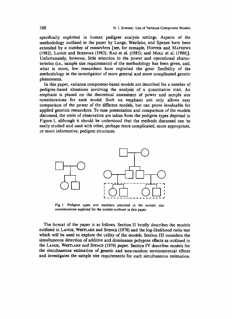
pedigree-based situations involving the analysis of a quantitative trait. An emphasis is placed on the theoretical assessment of power and sample size considerations for each model. Such an emphasis not only allows easy comparison of the power of the different models, but can prove invaluable for applied genetics researchers. To ease presentation and comparison of the models discussed, the units of observation are taken from the pedigree types depicted in Figure 1, although it should be understood that the methods discussed can be easily studied and used with other, perhaps more complicated, more appropriate, or more informative, pedigree structures.

Fig. 1. Pedigree types and members assumed in the sample sizc considerations explored for the models outlined in this paper.

The format of the paper is as follows. Section I1 briefly describes the models outlined in LANCE, WFSTLAKE and SPENCE (1976) and the log-likelihood ratio test which will be used to explore the utility of the models. Section 111 considers the simultaneous detection of additive and dominance polygene effects as outlined in the LANGE, WESTLAKE and SPENCE (1976) paper. Section IV describes models for the simultaneous estimation of genetic and non-random envir.onmenta1 effects and investigates the sample size requirements for such simultaneous estimation.

Biom. J. 35 (1993) 4 389

Section V considers models for pleiotropic gene action. Section VI considers models for aspects of the detection of polygenotype by environment interaction (ie., the detection of environmental sensitivity). Section VII describes sequential tests for variance component based genetic hypotheses of the type discussed in sections I1 to VI. Section VIII ends the paper with a brief discussion and a few summary remarks.

2. Pedigree Variance Component Models

Before describing the theoretical details of the test statistic studied in this paper, an explanation of the terms used to guide the sample size derivations will be offered for those readers whose only interest is to implement studies of the type outlined in this paper, and who do not want to concern themselves with the mathematics :

a-level. The a-level describes the probability of incorrectly rejecting a true hypothesis. One would want this probability to be set at some low-level (e.g., 0.05) in designing a study to test a specific hypothesis.

Power. The power of a test is a function of the probability of incorrectly accepting a false hypothesis. One would want the “power” of rejecting a false hypothesis to be quite high (e.g., 0.80 or 0.90) in applied settings.

Efficiency. Efficiency measures the relative sampling burden (i.e., how many data units must be collected to get reliable results) between two tests. A more ‘‘efficient” way to testing a hypothesis is one that requires a smaller data collection effort.

Sample size guideline. Sample size guidelines offer the average sampling one would need to undertake in order to reliably assess a specific hypothesis. This paper is confined to sampling pedigrees, and assumes that one will collect pedigrees of the same type (e.g., nuclear families with 2 offspring). Although rarely is this possible in practice, the guidelines based on a single type of pedigree do offer reasonable assessments of the sampling burden of a study which will collect pedigree types that do not deviate too much from the types used to build the guideline.

Consider a pedigree with n members where for each member, i, of the pedigree a quantitative trait, x i , has been collected. The x i can be collectively represented by the vector X = ( x i ) . Assume that X is multivariate normally distributed with mean vector p = (pl, p2,. . . , pn)’ and covariance matrix 8 (for a justification of the assumption of multivariate normality for multi-locus determined quantitative traits in pedigree contexts, see LANGE (1978)). Typically, p i = pj,Vi,j, though, following LANCE, WESTLAKE, and SPENCE (1976), one could assign mean values for the pedigree members based on concomitant information (e.g., sex). The covariance matrix, 8, includes components that relate possible sources of


variation to the possible pedigree members pairs’ relationships, and as such can be written, for example, as:

i2 = 2Kc: + DO: + H ct + I u ~ , (1)

where a:, c:, c;, uz, are the additive, dominance, shared environmental, and random environmental variances, respectively, associated with the trait in question. The other terms on the right hand side of equation (1) define the theoretical correlations between any two pedigree members given a relevant variance component. Thus, K is taken to be the Kinship coefficient matrix for the pedigree as it defines the theoretical correlations between pedigree members based on the amount of additive genetic information they share (JACQUARD, 1974); D is Jacquard’s condensed coefficient of identity matrix, d, (JACQUARD, 1974); H is a matrix that defines which pedigree members actually share the same environment and/or to what degree they share this environment (see section IV); and I is the identity matrix. To compute estimates of the mean vector p, and the components of 0, given data xk collected on N pedigrees (k = 1,. . . , N), possibly of different sizes and structures, one can maximize the relevant log-likelihood function, which is, apart from a constant:

N - 1 1 L(c:, c62, ct, c:, xN)= (2)

k = l

To draw inferences about a certain variance component parameter, E 8 = = (u:, a;, c;, cz), standard likelihood ratio statistics, tLR, involving hypotheses of the form Ho : dl = 0 vs. If, : 8, > 0 can be computed and assigned probabilities.

It is well known that under the alternative hypothesis, If,, t,, is asymptotic- ally distributed as non-central x 2 with non-centrality parameter:

(3)

where 1, is the information matrix of the parameters evaluated under the null hypothesis and 8, and Oo are the parameter vectors under the alternative and null hypotheses, respectively. Given N similarly structured pedigrees, the power of the likelihood ratio test given relevant null and alternative hypothetical para- meterizations can be obtained from:

1 = (6, - 6,)’ Ip(4 - 601,

where xtZ is the non-central x 2 with non-centrality parameter

1, = (61 - O O Y (N * 1,) (6, - 4J; df is the number of degrees of freedom; and where q,, is the.appropriate ath quantile of a x2 distribution with df degrees for the assumed test level. The

Biom. J. 35 (1993) 4 39 1

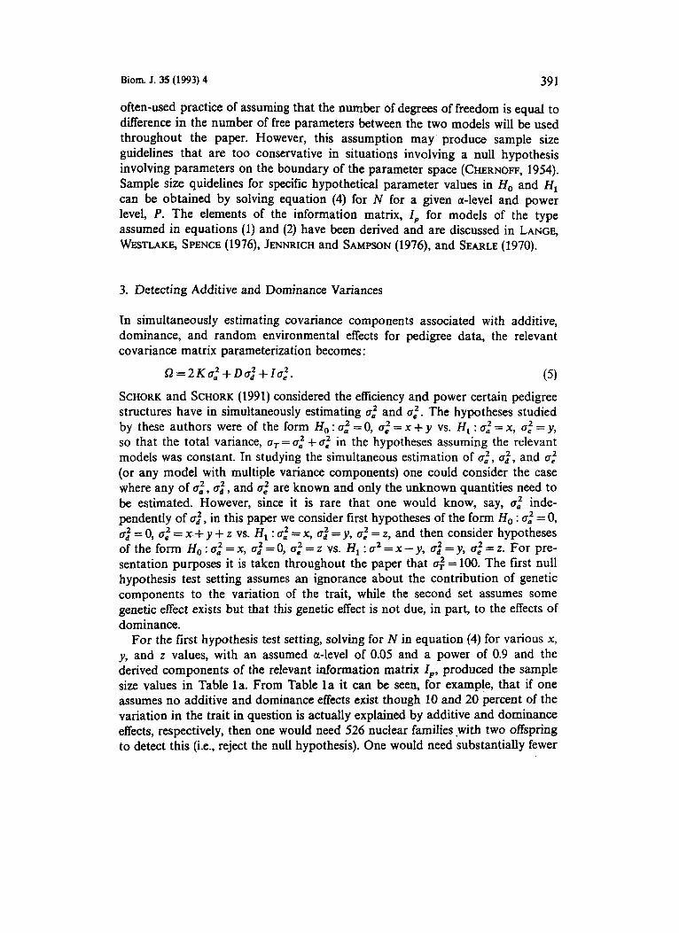
often-used practice of assuming that the number of degrees of freedom is equal to difference in the number of free parameters between the two models will be used throughout the paper. However, this assumption may produce sample size guidelines that are too conservative in situations involving a null hypothesis involving parameters on the boundary of the parameter space (CHERNOFF, 1954). Sample size quidelines for specific hypothetical parameter values in H, and If, can be obtained by solving equation (4) for N for a given a-level and power level, P. The elements of the information matrix, I p for models of the type assumed in equations (1) and (2) have been derived and are discussed in LANCE, WESTLAKE, SPENCE (1976), JENNRICH and SAMPSON (1976), and SEARLE (1970).

3. Detecting Additive and Dominance Variances

In simultaneously estimating covariance components associated with additive, dominance, and random environmental effects for pedigree data, the relevant covariance matrix parameterization becomes:

SZ = 2 K 0,' + D 0; + ID,'. (5 ) SCHORK and SCHORK (1991) considered the efficiency and power certain pedigree structures have in simultaneously estimating cr,' and cr,' . The hypotheses studied by these authors were of the form H , : 0,' = 0, cr,' = x + y vs. H , : 0,' = x, cr,' = y, so that the total variance, crT = cr,' + cr,' in the hypotheses assuming the relevant models was constant. In studying the simultaneous estimation of cr:, crf, and cr,' (or any model with multiple variance components) one could consider the case where any of cr,' , cr; , and cr," are known and only the unknown quantities need to be estimated. However, since it is rare that one would know, say, u,' inde- pendently of cr; , in this paper we consider first hypotheses of the form Ho : cr,' = 0, crf = 0, cr," = x. + y + z vs. HI : cr,' = x, cr: = y, cr," = z, and then consider hypotheses of the form H , : cr,' = x, cr; = 0, 0," = z vs. Ifl : cr2 = x- y, cr: = y, c," = z. For presentation purposes it is taken throughout the paper that cr; = 100. The first null hypothesis test setting assumes an ignorance about the contribution of genetic components to the variation of the trait, while the second set assumes some genetic effect exists but that this genetic effect is not due, in part, to the effects of dominance.

For the first hypothesis test setting, solving for N in equation (4) for various x, y, and z values, with an assumed a-level of 0.05 and a power of 0.9 and the derived components of the relevant information matrix I p , produced the sample size values in Table la. From Table la it can be seen, for example, that if one assumes no additive and dominance effects exist though 10 and 20 percent of the variation in the trait in question is actually explained by additive and dominance effects, respectively, then one would need 526 nuclear families .with two offspring to detect this (i.e., reject the null hypothesis). One would need substantially fewer


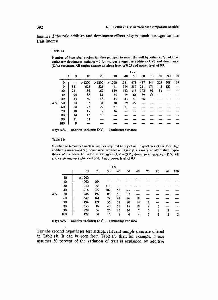
families if the role additive and dominance effects play is much stronger for the trait interest.

Table la

Number of Cmember nuclear families required to reject the null hypothesis H,: additive variance = dominance variance = 0 for various alternative additive (A.V.) and dominance (D.V.) variances. All entries assume an alpha level of 0.05 and power level of 0.9.

D.V. I 0 10 20 30 40 50 60 70 80 90 100

~~

0 10 20 30 40

A.V. 50 60 70 80 90

100

- 84 1 21 1 94 53 34 24 18 14 11 9

>1200 >1200 >1200 1051 673 467 344 673 526 411 324 259 211 174 189 169 149 132 116 ,103 91 88 81 75 69 64 59 54 50 48 45 43 40 38 - 33 31 30 29 27 - - 23 22 21 21 - - - 17 17 13 13 11

16 _ _ _ _ - - - - -

- - - - - -

263 145 81 -

208 123 -

169 -

Key: A.V. - additive variance; D.V. - dominance variance

Table 1 b

Number of 4-member nuclear families required to reject null hypotheses of the form H,: additive variance = A.V.; dominance variance = 0 against a variety of alternative hypotheses of the form HI : additive variance = A.V. - D.V.; dominance variance = D.V. All entries mume an alpha level of 0.05 and power level of 0.9

D. V. I 10 20 30 40 50 60 70 80 90 100

10 20 30 40

A.V. 50 60 70 80 90

100

> 1200 I060 1010 914 786 642 494 353 229 128

- - - 265 - - 253 113 - 229 102 58 197 88 50 161 72 41 124 55 31 89 40 23 58 26 15 32 15 8

- 32 26 20 15 10 6

- 18 14 10 7 4

11 8 s 3

- 6 4 2

3 2

-

2

Key: A.V. - additive variance; D.V. - dominance variance

\ For the second hypotheses test setting, relevant sample sizes are offered in Table 1b. It can be seen from Table l b that, for example, if one assumes 50 percent of-the variation of trait is explained by additive

Biom. J. 35 (1993) 4 393

effects and none of the variation of the trait is explained by dominance effects although only 40 percent of the variation in the trait is actually determined by additive effects with 10 percent actually determined by dominance effects, then one would need 786 two-offspring nuclear families to detect this. The number of families required to reject the hypothesis that 50 percent of the variation in the trait is controlled by additive effects is reduced markedly as dominance effects account for greater amounts of the variation in the trait.

4. Detecting Additive and Non-Random Environmental Variances

It is rarely the case in humans that no non-random environment factors are of consequence to the variation of a specific quantitative trait. In addition, it is very easy to mistake shared environmental effects (e.g., dietary or smoking practice within a household) for genetic effects. Thus, the simultaneous estimation of non-random environmental sources of variation in the presence of genetic sources, and vice versa, is an extremely important undertaking if one is to properly identify the sources influencing the expression of a trait. In the context of the models for pedigrees outlined in section 11, a simple model positing additive genetic and non-random environmental effects would have covariance structure:

SZ = 2 K c,‘ + H 0; + 10,‘. (6)

Specification of the matrix H is essential since it must be constructed in such a way that, when used in equation (6), it produces a true covariance matrix (e.g., it preserves positive-definiteness, etc.) while still quantifying the effects of interest. In this paper we consider the elaboration and design of H as given in the formulation of the “shared sibling” and “parent-offspring” environmental effects described in ASTEMBORSKI et al. (1985). Basically, ASTEMBORSKI et al. (1985) define an n x n matrix, R, for a pedigree or household whose (i, j)th component is 1 if member i is an offspring of member j and 0 if not. The pedigree’s shared sibship environment is then characterized by the matrix H, given by:

H,=RR‘+ I , (7 a)

and the shared parent-offspring environment is characterized by the matrix H p given by:

Hp = ( R + I ) ( R + I ) ’ . (7 b)

Given these constructions of a non-random environmental effect, at least three hypothesis test settings can be formed. First, one can assume that no shared sibling environment effect exists, although an additive genetic effect does. This situation can be reversed, where one assumes no additive genetic effect exists,


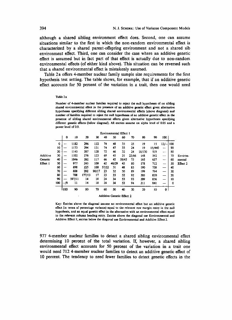
although a shared sibling environment effect does. Second, one can assume situations similar to the first in which the non-random environmental effect is characterized by a shared parent-offspring environment and not a shared sib environment effect. Third, one can consider the case where an additive genetic effect is assumed but in fact part of that effect is actually due to non-random environmental effects (of either kind above). This situation can be reversed such that a shared environmental effect is mistakenly assumed.

Table 2a offers 4-member nuclear family sample size requirements for the first hypothesis test setting. The table shows, for example, that if an additive genetic effect accounts for 50 percent of the variation in a trait, then one would need

Table 2 a

Number of Cmember nuclear families rquired to reject the null hypotheses of no sibling shared environmental effect in the prcsena of an additive genetic effect given alternative hypothcsn, specifying diflerent sibling shared environmental effects (above diagonal) and number of families required to reject the null hypotheses of no additive genetic effect in the presence of sibling s h a d environmental effects given alternative hypotheses specifying different genetic effects (below diagonal). All entries assume on alpha level or 0.05 and a power level of 0.9.

Environmental Effect I 1 0 10 20 30 40 50 60 70 80 90 1001

0 10 20

Additive 30 Genetic 40 Effect 1 50

60 70 80 90

100 -

1182 1173 1145 1102 1046 977 898 808 708

59711 1 11

90

296 294 287 276 262 245 225 202

177113 14 14

80

132 74 48 33 131 74 47 33 128 72 46 32 123 69 45 31 117 66 42 30142 109 62 4 /29 45 100 57/22 31 48

90117 23 32 50 17 23 33 52 18 24 34 53 18 24 34 53

7 0 6 0 5 0 4 0

25 24 24

23/66 73 80 85 89 92 93 94

30 -

19 19

18/130 I48 165 I78 190 I99 205 209 21 1

20

15 I5/440

519 592 657 712 758 794 820 836 84 I

10 -

100 90 80 70 Environ- 60 mental 50 Effect2 40 30 20 10 0

Additive Genetic Effect 2

Key: Entries above the diagonal w u m e no environmental effect but an additive genetic effect (in terms of percentage variance) q u a l to the relevant row margin entry in the null hypothesis, and an q u a l genetic effect in the alternative with an environmental effect q u a l to the relevant column heading entry. Entries above the diagonal use Environmental and Additive Effect 1; entries below the diagonal use Environmental and Additive Effect 2.

977 4-member nuclear families to detect a shared sibling environmental effect determining 10 percent of the total variation. If, however, a shared sibling environmental effect accounts for 50 percent of the variation in a trait one would need 712 4-member nuclear families to detect an additive genetic effect of 10 percent. The tendency to need fewer families to detect genetic effects in the

Biom. J. 35 (1993) 4 395

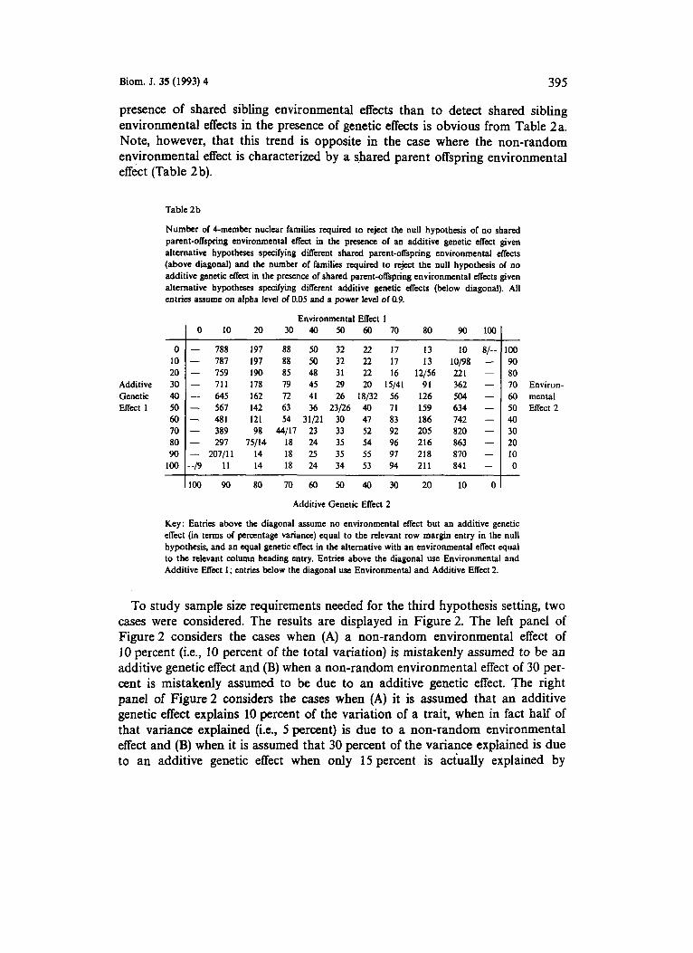
presence of shared sibling environmental effects than to detect shared sibling environmental effects in the presence of genetic effects is obvious from Table 2a. Note, however, that this trend is opposite in the case where the non-random environmental effect is characterized by a shared parent offspring environmental effect (Table 2 b).

Table 2 b

Number of Cmembet nuclear families required to reject the null hypothesis of no shared parent-offspring environmental effect in the presence of an additive genetic effect given alternative hypotheses specifying dflerent shared parent-offspring environmental effects (above diagonal) and the number of families required to reject the null hypothesis of no additive genetic effect in the presence of shared parent-offspring environmental effects given alternative hypotheses specdying different additive genetic effects (below diagonal). All entries w u m c on alpha level of 0.05 and a power level of 0.9.

- 0

10 20

Additive 30 Genetic 40 Effect I 50

60 70

90 100

ao

-

0 10

- 788 787 -

- 759 71 1

- 645 - 567 - 481

- 297 - 207111 -p 11

-

- 389

20

197 197 190 178 162 142 121

75/14 14 14

98

Environmental Effect 1 30 40 50 60 70

88 50 32 22 17 88 50 32 22 17 85 48 31 22 16 79 45 29 20 15/41 72 41 26 18/32 56 63 36 23/26 40 71

44/17 23 33 52 92 18 24 35 54 96 18 25 35 55 91

54 31/21 30 47 a3

la 24 34 53 94

ao

13 13

12/56 91

126 159

205 216 218 21 1

186

90

10

22 I 362 504 634 742

863 810 841

lopa

a20

100 90 80 70 60 50 40 30 20 10 0

Additive Genetic Erect 2

- 00 90

70 Environ- 60 mental 50 Effect 2 40 30 20 I0 0

ao

-

Key: Entries above the diagonal assume no environmental effect but an additive genetic effect (in terms of percentage variance) equal to the relevant row margin entry in the null hypothesis, and an equal genetic effect in the alternative with an environmental effect equal to the relevant column heading entry. Entries above the diagonal use Environmental and Additive Effect 1; entries below the diagonal use Environmental and Additive Effect 2.

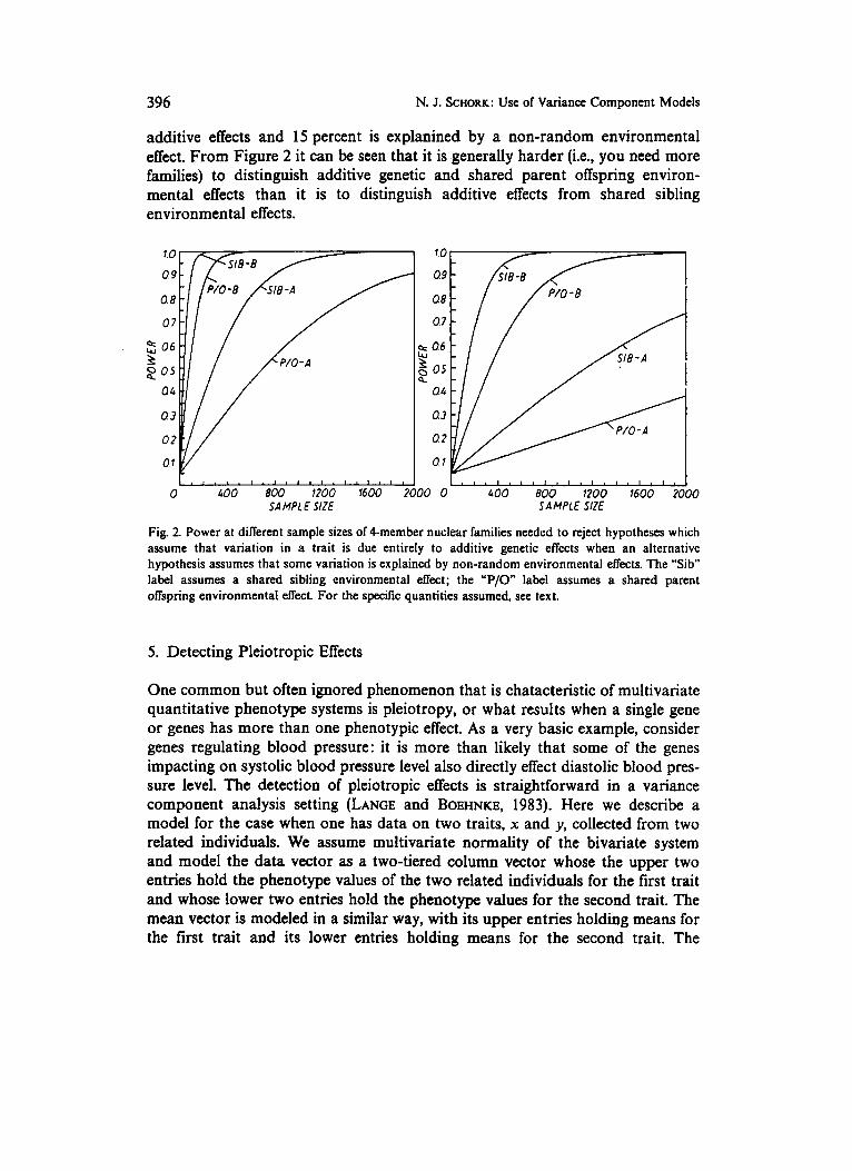
To study sample size requirements needed for the third hypothesis setting, two cases were considered. The results are displayed in Figure 2. The left panel of Figure 2 considers the cases when (A) a non-random environmental effect of 10 percent (ie., 10 percent of the total variation) is mistakenly assumed to be an additive genetic effect and (B) when a non-random environmental effect of 30 percent is mistakenly assumed to be due to an additive genetic effect. The right panel of Figure2 considers the cases when (A) it is assumed that an additive genetic effect explains 10 percent of the variation of a trait, when in fact half of that variance explained (i-e., 5 percent) is due to a non-random environmental effect and (B) when it is assumed that 30 percent of the variance explained is due to an additive genetic effect when only 15 percent is actually explained by


additive effects and 15 percent is explanined by a non-random environmental effect. From Figure 2 it can be seen that it is .generally harder (i.e., you need more families) to distinguish additive genetic and shared parent offspring environmental effects than it is to distinguish additive effects from shared sibling environmental effects.

30

Fig. 2. Power at different sample sizes of 4-member nuclear families needcd to reject hypotheses which assume that variation in a trait is due entirely to additive genetic etTects when an alternative hypothesis assumes that some variation is explained by non-random environmental effects. The "Sib" label assumes a shared sibling environmental effect; the "P/O label assumes a shared parent oNspring environmental effect. For the specific quantities assumed, see text.

5. Detecting Pleiotropic Effects

One common but often ignored phenomenon that is chatacteristic of multivariate quantitative phenotype systems is pleiotropy, or what results when a single gene or genes has more than one phenotypic effect. As a very basic example, consider genes regulating blood pressure: it is more than likely that some of the genes impacting on systolic blood pressure level also directly effect diastolic blood pressure level. The detection of pleiotropic effects is straightforward in a variance component analysis setting (LANGE and BOEHNKE, 1983). Here we describe a model for the case when one has data on two traits, x and y, collected from two related individuals. We assume multivariate normality of the bivariate system and model the data vector as a two-tiered column vector whose the upper two entries hold the phenotype values of the two related individuals for the first trait and whose lower two entries hold the phenotype values for the second trait. The mean vector is modeled in a similar way, with its upper entries holding means for the first trait and its lower entries holding means for the second trait. The

Biom. J. 35 (1993) 4 397

covariance matrix, s2, is modeled as the sum of a series of “block” or partitioned matrices (LANCE and BOEHNKE, 1983; RAO, 1973) whose blocks hold information associated with one of the two traits. For example, a model assuming additive genetic effects and a random environmental component could be written as :

where a:l and a:2 are the additive genetic variance components for the first and second traits, respectively; . 2 is the additive genetic covariance component for the two traits; and where a:l and are the environmental variance components associated with the first and seconds traits, respectively. A more realistic model may posit a non-random, environmental effect for the traits as well as a non-random environmental covariance between the two traits (LANCE and BOEHNKE, 1983). Of interest is the term a:l,2 which can be associated with the effects of pleiotropic gene action in that it represents genetic sources of variation that act on both traits simultaneously.

We explored the sample size requirements necessary to pick up a pleiotropic effect (i-e., CT:~.,>O) for the two cases in which data on two different traits has been collected from sibling pairs and cousin pairs (ie., two related individuals).

In the first case we assumed that the genetic effects were equal for the two traits. The results are displayed in Figure 3. The left panel of Figure 3 presents

I I . I I l . I I ,

0 100 200 300 400 500 0 100 200 300 400 500 SAMPLE SIZE SAMPLE SIZE

Fig. 3. Power at different sample sizes in the detection of pleiotropic efkts, when the null hypothesis assumes that no such effect exists, though some additive effect does exist for each of 2 traits. For a discussion of what efTects are assumed, see text. The “Cousins” label assumes sample size calculations made use of the number of genes shared identical by descent by two cousins; the “Sibs” label assumes sample size calculations made use of the number of genes shared identical by descent by two sibs.


results associated with (A) the null hypothesis of no genetic effects (i.e., Ho : = a:; .1 = 0; ac', = azz = 100) as against the alternative hypothesis H, : a:l = a:l = a:l.l = 20; ac', = azZ = 60 and (B) the null hypothesis of no genetic effects against the alternative HI = a:l = 4.22 = a:; . 2 = 10; af, = az2 = 80. The right panel of Figure 3 presents results when the null hypothesis assumes that some additive effect exists for each trait but also that the traits are independent against the alternative that an equal amount of each additive effect variance contribution is actually the result of pleiotropic effects on the two traits. Two cases are displayed: (A) the null Ho : dl = ofz = 40; ail , l = 0; = azz = 60 against the alternative H, : = 6.22 = 20; a:, , = 20; oe", = azz = 60 and (B) the null Ho : = 0.2, = a:z = 20; dl .1 = 0; ac', = azl = 80 against the alternative H, : a:l = cr22 = = 10;

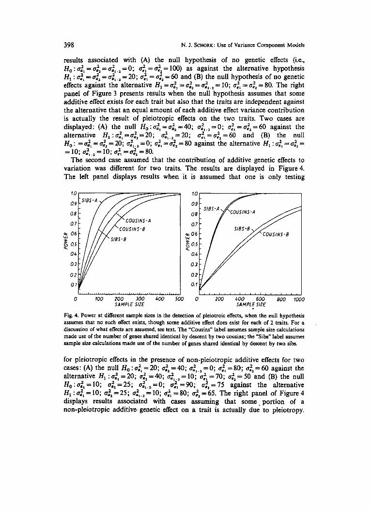
The second case assumed that the contribution of additive genetic effects to variation was different for two traits. The results are displayed in Figure 4. The left panel displays results when it is assumed that one is only testing

=

2 2 , z = 10; gel = gel = 80.

0 100 200 300 600 500 0 200 600 600 800 1000 SAMPLE SIZE SAMPLE SIZE

Fig. 4. Power at different sample sizes in the detection of pleiotroic eNects, when the null hypothesis assumes that no such effect exists. though some additive eNect does exist for each of 2 traits. For a discussion of what eNects are assumed, see text. The "Cousins" label assumes sample size calculations made use of the number of genes shared identical by descent by two cousins; the "Sibs" label assumes sample size calculations made use of the number of genes shared identical by descent by two sibs.

for pleiotropic effects in the presence of non-pleiotropic additive effects for two cases: (A) the null Ho : a:; = 20; a:l= 40; azl .1 = 0; aL", = 80; a.22 = 60 against the alternative HI : a:l = 20; a.22 = 40; u:l.l = 10; atl = 70; azl = 50 and (B) the null Ho : 002, = 10; = 25; a:l.2 = 0; c ~ : ~ = 90; atl = 75 against the alternative H , : ail = 10; a:z = 25; a:l.z = 10; ac", = 80; azz = 65. The right panel of Figure 4 displays results associated with cases assuming that some portion of a non-pfeiotropic additive. genetic effect on a trait is actually due' to pleiotropy.

Biorn. J. 35 (1993) 4 399

Again, two cases were studied: (B) the null H, : cZl = 20; o:~ = 40; a.2,,z = 0; C J ~ , = 80; = 60 against the alternative HI : 0.21 = 10; 0.22 = 25; 0.2, .z = 10; 0,2,=80; ~ ~ : ~ = 6 5 and (B) the null H , : 0 ~ ~ = 1 0 ; atZ=25; a.Z,.,=O; ~ e ' , =90; a:2 = 75 against the alternative H, : 0.21 = 5 ;

From Figures 3 and 4 it can be seen that generally, as expected, siblings pairs provide more information than cousin pairs in the detection of pleiotropic effects; although what is interesting in these two figures is that this difference is diminished when one already assumes some additive genetic effect for two traits exists and merely wants to test to see if this effect is not actually due to, in part, to pleiotropy (the right panels of Figures 3 and 4 vs. the left panels).

= 20; = 5 ; no', = 90 ; oZ2 = 70.

6. Detecting Differential Environmental Effects

One particularly interesting genetic phenomenon which is difficult to quantify and test in the context of human quantitative traits involves genetic/environmental interactions. Although some methodological research in this area has been published (see sections 44 through 46 of WEIR et.al. (1988) for a discussion and references), not much of it can be readily applied to human quantitative trait analysis. In a pedigree context one could model the pedigree trait vector, X, as:

X = G + E + ( G * E ) , (9)

where G and E are the genetic and environmental effects and (G. E) is the genotype by environment interaction term. From equation (9) one could con- struct relevant covariance terms. However, some problems with this construction are that it assumes an unequivocal knowledge of the genotype of each individual and that each possible genotype is represented in each environment. Such a construction would be virtually impossible in contexts involving human quantitative traits with polygenic bases.

As an alternative we consider the following design. One has measurements collected on two (supposedly) genetically disparate populations. For each population one has measurements collected on subgroups of people from different environments. One then estimates the genetic and environmental effects (e.g., through variance component analysis) within each population and then investigates possible differential effects of the environment on the trait of interest between the populations. If such differential effects exist, they may represent the effects of gene by environment intraction. Consider the following example sce- nario where blood pressure is the variable of interest. Blood pressure data has been collected from two different ethnic or race groups. Half of the data for each race or ethnic group is collected from people with high salt diets and the other half from people with low salt diets. With this data, genetic variance and non-random environment parameters are estimated with the hope of showing that the high


salt diet has a greater (or lesser) effect on blood pressure in one of the two populations, regardless of differences in the total amount of variability in blood pressure explained by genetic effects that may exist between the two populations (although these differences may reflect the known genetic differences between the populations). Many assumptions are built into this setting; such as that the diets are the same, no unmeasured environmental variable impacts on the differences between the populations, etc.

One important aspect of the setting described above is the detection of the difference in the effects the two environments have on the trait of interest for the populations. It is this environmental sensitivity (FALCONER, 198 1) which is explored in the following. We consider data collected on two sets of sib pairs that are related to each other as cousins (see Figure 1, right panel, bottom-most individuals) so that all 4 members in this observation unit share genetic information. It is assumed that the sib pairs live in different environments. The covariance matrix for this “cousin-set” unit of observation can be written as:

8 = 2Ka,” + H, ah‘, + HZatz + I a,”. (10)

H , and H , are block matrices of the type described in section V. H, is non-zero for only those entries relating to the sib pair members living in environment 1. The non-zero entries are then given, numerically, as that number which charac- terizes a shared sibling environment effect as defined in equation (7a). Such non- zero entries are given in the entries of matrix H, for the sib pair which resides in environment 2.

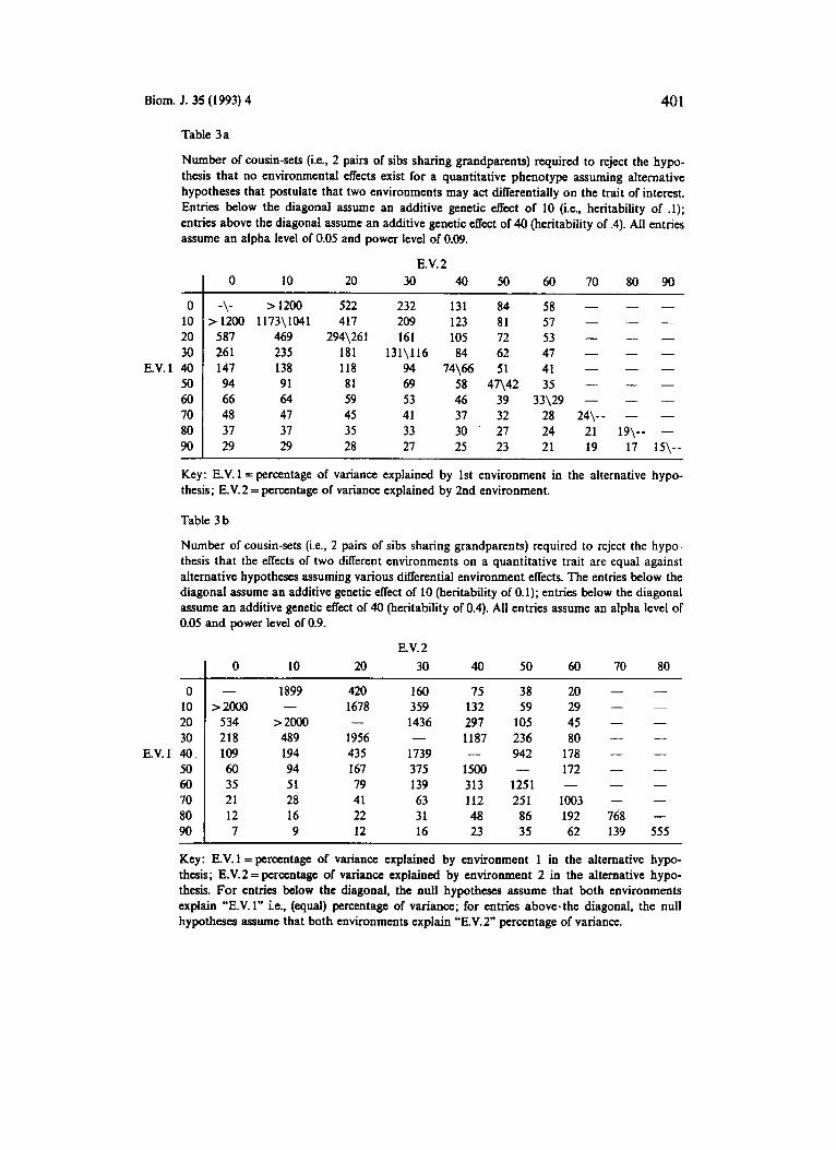
Two hypothesis settings were investigated. The first setting posited the null hypothesis, Ho : a,” = x; ail = at, = 0; a,‘ = y, + y, + z against alternatives of the form HI : c,” = x ; uh’, = y, ; aiz = y,; a,‘ = z. The number of cousin sets required to reject the null hypothesis at given alternatives for this setting is described in Table 3 a. The second setting posited the null hypothesis, Ho : a,” = x; ah’, = y, ;

a, = z . The sample size requirements for settings of this type are described in Table 3 b.

From Table 3a and 2b it can be seen that it is easier to pick up differential environmental effects when a greater portion of the variability of the trait is accounted for by genetic effects.

a:, = y, ; a,” = y, + z against alternatives of the form HI : a,” = x; ahl 2 = y, ; a,,, 2 = p,;

7. Sequential Variance Component Testing

In the previous sections of this paper, an emphasis has been placed on the formation of, and sample size considerations associated with, variance component models used to detect genetic and complementary effects. One possible strategy one could employ to reduce the sampling effort required to detect the effects

Biom. J. 35 (1993) 4 401

Table 3a

Number of cousin-sets (i.e.. 2 pairs of sibs sharing grandparents) required to reject the hypothesis that no environmental effects exist for a quantitative phenotype assuming alternative hypotheses that postulate that two environments may act diflerentially on the trait of interest. Entries below the diagonal assume an additive genetic effect of 10 (i.e., heritability of .l); entries above the diagonal assume an additive genetic effect of 40 (heritability of .4). All entries assume an alpha level of 0.05 and power level of 0.09.

- 0

10 20 30

E.V.l 40 50 60 70 80 90

0

-\- > 1200

587 26 1 147 94 66 48

10 E.V. 2

20 30 40 50 60 70 80 90

> 1200 1173\ 1041

469 235 138 91 64 47 37 29

522 232 417 209

294\261 161 181 131\116 118 94 81 69 59 53 45 41 35 33 28 27

131 123 105 84

74\66 58 46 37 30 25

84 81 72 62 51

47\42 39 3 32 21 23

58 57 53 47 41 35

;3\29 28 24 21

- - - 24\-- - -

21 19\-- - 19 17 15\--

Key: E.V. 1 =percentage of variance explained by 1st environment in the alternative hypothesis; E.V.2 = percentage of variance explained by 2nd environment.

Table 3 b

Number of cousin-sets (i.e., 2 pairs of sibs sharing grandparents) required to reject the hypothesis that the effects of two different environments on a quantitative trait are equal against alternative hypotheses assuming various differential environment effects. The entries below the diagonal assume an additive genetic effect of 10 (heritability of 0.1); entries below the diagonal assume an addkive genetic effect of 40 (heritability of 0.4). All entries assume an alpha level of 0.05 and power level of 0.9.

- 0

10 20 30

E.V.1 40 50 60 70 80 90

0 10 20 E.V. 2

30 40 50 60 70 80

- > 2000

534 218 109 60 35 21 12 7

1899

> 2000 489 194 94 51 28 16 9

- 420 1678

1956 435 167 79 41 22 12

-

160 359 1436

1739 375 139 63 31 16

-

75 132 297 1187

1500 313 112 48 23

-

38 59

105 236 942

1251 251 86 35

-

20 29 45 80

178 172

1003 192 62

-

768 139

- 555

Key: E.V. 1 =percentage of variance explained by environment 1 in the alternative hypothesis; E.V.2=percentage of variance explained by environment 2 in the alternative hypothesis. For entries below the diagonal, the null hypotheses assume that both environments explain “E.V. 1” i.e., (equal) percentage of variance; for entries aboveathe diagonal, the null hypotheses assume that both environments explain “E.V.2” percentage of variance.

402 N. J. SCHORK: Use. of Variance Component Models

described would be to carry out relevant tests sequentially as the data arrive in an effort to stop the sampling process when conclusive evidence for one of two hypotheses has been obtained. Although many sequential test constructions exist which can be applied to the models outlined in this paper, in this section we consider the use of Cox’s classic sequential probability ratio test (1963), which is appropriate for the models described so far because of its consideration of nuisance parameters.

Cox (1963) considered the properties of the repeated use of the likelihood ratio test:

where O2 and 8, are the values of the parameter to be tested under the two hypotheses, 4 is a nuisance parameter, and L, is a log-likelihood evaluated with 8 set to O1 or 8,. Cox (1963) showed that if one computes the maximum likelihood estimates, 6 and 6, a test statistic, t,, can be derived from the formation of t,, as:

The stopping limits, s1 and s,, for the repeated application of t, were also given by Cox (1963), assuming type I and type I1 error rates of a and by respectively:

where Zee is a simple manipulation of the components of the relevant Information matrix and is defined in equation 2.10 in Cox (1963). Cox (1963) also offered an expression for the “operating characteristic” of the test which gives, essentially, error probabilities associated with the application of the test, as well as an expression for computing the expected sample size requirements for the test.

Consider the use of Cox‘s test in assessing the significance of additive genetic effects on a trait of interest where 4-member nuclear families will be sampled repeatedly until some conclusion about this additive genetic effect has been reached: the parameter of interest, 8, is taken to be the additive variance component; the mean parameter and random environmental variance component are considered nuisance parameters, 4. As such, one would compute t, for 8 = n.’ after each family has been sampled. If at any time the computed t, is less than sly one sides with hypothesis 1, Hl : 8= 8,; if t , is greater than s,, one sides with hypothesis 2, H2 : e^= 02. If t, satisfies neither s, or s,, then one continues sampling. An experiment was performed to explore the utility of the Cox test in the

detection of additive genetic effects. 200 replications of simulated data samplings of 4-member nuclear families were performed assuming different hypothetical O1 and O2 values for different values of the “true” 0 value. Sink in the models

Biom. J. 35 (1993) 4 403

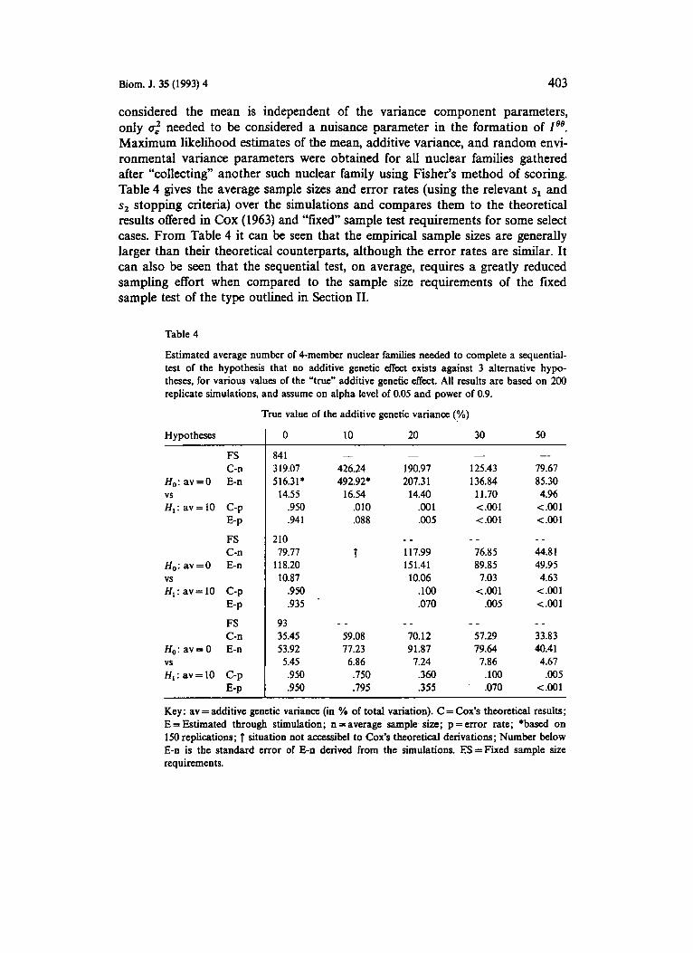
considered the mean is independent of the variance component parameters, only u,” needed to be considered a nuisance parameter in the formation of 1’’. Maximum likelihood estimates of the mean, additive variance, and random environmental variance parameters were obtained for all nuclear families gathered after “collecting” another such nuclear family using Fisher’s method of scoring. Table 4 gives the average sample sizes and error rates (using the relevant s1 and s2 stopping criteria) over the simulations and compares them to the theoretical results offered in COX (1963) and “fixed” sample test requirements for some select cases. From Table 4 it can be seen that the empirical sample sizes are generally larger than their theoretical counterparts, although the error rates are similar. It can also be seen that the sequential test, on average, requires a greatly reduced sampling effort when compared to the sample size requirements of the fixed sample test of the type outlined in Section 11.

Table 4

Estimated average number of 4-member nuclear families needed to complete a sequential- test of the hypothesis that no additive genetic effect exists against 3 alternative hypotheses, for various values of the “true” additive genetic effect. All results are based on 200 replicate simulations, and assume on alpha level of 0.05 and power of 0.9.

True value of the additive genetic variance (%)

Hypotheses I 0 10 20 30 50

FS C-n

H,: av=O E-n

HI: av= 10 C-p vs

E-P

FS C-n

H,:av=O E-n

H,: av=10 C-p vs

E-P

FS C-n

H,,: a v = O E-n

HI: av=10 C-p E-P

vs

84 I 3 19.01 5 16.3 1 * 14.55 .950 .941

210 19.11 118.20 10.87 .950 .935 ’

93 35.45 53.92 5.45 .950 .950

- 426.24 492.92* 16.54 .010 .088

7

- - 59.08 77.23 6.86 .750 .795

-

190.97 207.3 1 14.40 .oo 1 .005

- - 1 17.99 151.41 10.06 .loo .070

- - 70.12 91.87 1.24 .360 .355

- 125.43 136.84 11.70 <.001 <.W1

- - 76.85 89.85 1.03 < .001 .005

- - 51.29 79.64 1.86 .loo .070

- 19.61 85.30 4.96

<.001 <.001 - - 44.8 1 49.95 4.63 <.001 <.001 - - 33.83 40.4 1 4.61

.005 <.001

I

Key: av = additive genetic variance (in % of total variation). C = Cox’s theoretical results; E = Estimated through stimulation; n = average sample. size; p = error rate; *based on 150 replications; 1 situation not accessibel to Cox’s theoretical derivations; Number below E-n is the standard error of E-n derived from the simulations. ES=Fixed sample site requirements.


8. Discussion

As noted in the Introduction, the use of variance component models in the analysis of human quantitative phenotypes is common despite the fact that not much theoretical work exists which either extends the more basic models to more complex situations or studies the operating characteristics of extant models. This paper was meant to be a first step in remedying this situation. As a first step, however, it naturally presents some flaws or directions for further research. For instance, it would be beneficial to investigate the information that different pedigree types offered in the investigation of each of the settings touched on this paper, much in the way SCHORK and SCHORK (1991) did for the case of detecting additive genetic effects. In addition, it is also important to consider the effects on sample size requirements that the collection of "mixed" samples (i.e., pedigrees of different sizes and complexity) would have, since this setting is much more realistic than the exclusive collection of any single type of pedigree.

Another area of great contemporary interest relevant to the studies outlined in this paper is the role and detection of "major" genes (i.e., single genes with large phenotypic effects) in contexts of dominance, pleiotropy, and gene by environment interaction. The detection of such genes through statistical means is generally seen as a precursor to the genomic isolation of these genes and as such could aid in the detection and correction of disease genes.

Ultimately, however, if genetics researchers are to progress in their understand- ing of quantitative phenotype expression as an aid to unraveling evolutionary factors, the determinants of disease, the impact of the environment on different species, etc. it behooves them to consider the proper derivation and use of models expressly designed for purposes consistent with their own.

ReJerences

ASTIWEORSKI, J. A.. BEMY, T. H., and COHEN, B. H., 1985: Variance components analysis of forced

CHERNOFP, H., 1954: On the distribution of the likelihood ratio. Ann. Math. Statist. 25, 573-578. Cox, D. R., 1963: Large sample sequential tests for composite hypotheses. Sankhya 25, 5-12. FALCONER, D. S., 1981: Introduction to Quantitative Genetics. New York: Ronald Press. FISHER, R. A., 1918: The correlation between relatives on the supposition of Mendelian inheritance.

HOPPEX, J. L., and MATHEWS, J. D., 1982: Extensions to multivariate normal models for pedigree

JACQUARD, A.. 1974: The Genetic Structure of Populations. New York: Springer. JENNRICH, R. L.. and S A h c p s o ~ , P. F., 1976: Newton-Raphson and related algorithms for maximum

likelihood variance component estimation. Technometria 18, 11-17. KEMpMoRNE, 0.. 1957: An Inh.oduction to Genetic Statistics. New York: John Wiley. LANGE, Ic, 1978: Central limit theorems for pedigrees. J. Math. Biol. 6, 59-66. LANGE, K., and BOEHNKE, M., 1983: Extensions to pedigree analysis. IV. Covariance components

expiration in families. Amer. J. Med. Genetics 21, 741-753.

Transactions of the Royal Society of Edinburgh 52, 399-433.

analysis. Ann. Human Genet. 46, 373-383.

models for multivariate traits. Amer. J. Med. Genet. 14, 513-524.

Biom. J. 35 (1993) 4 405

LANCE, K., WESTLAKE. J., and SPENCE, M. A., 1976: Extensions to pedigree analysis. 111. Variance components by the scoring method. Ann. .Human Genet. 4, 171-189.

MOLL, P. P., POWSNER, R., and SING, C. F., 1979: Analysis of genetic and environmental sources of serum cholesterol in Tecumseh, Michigan. V. Variance. components estimated from pedigree. Ann. Human Genet. 42, 343-354.

RAO. C. R., 1973: Linear Statistical Inference and its Applications. 2nd Ed. New York: John Wiley. RAO. D. C.. VOGLEX, G. P., MCGUE, M., RUSSELL, J. M., 1987: Maximum likelihood estimation of

familial correlations from multivariate quantitative data on pedigrees: a general method and examples. Amer. J. Human Genet. 41, 1104-1116.

SCHORK, N. J., and SCHORK, M. A., 1993: The relative elficiency and power of small pedigree studies of the heritability of a quantitative trait. (in press) Human Heredity.

SWRLE, S. R., 1970: Large sample variances of maximum likelihood estimators of variance components using unbalanced data. Biometrin 26, 505-524.

WEIR, B. S., GOODMAN, M. M., EISEN, E. J., and NAMKOONG, G. (eds.), 1988: Proceedings of the Second International Conference on Quantitative Genetics. Massachusetts: Sinauer Associates, Inc.

Received: Jan. 1992 Revised: April 1992

NICHOLAS J. SCHORK Department of Internal Medicine and Department of Epidemiology University of Michigan Ann Arbor Michigan 48109-0500 U.S.A.

the design and use of variance component models in the analysis of human quantitative pedigree data

Documents