the co2 greenhouse effect and the thermal history of the atmosphere

Adv. Space See. Vol.1, pp.S—l8. 0273_1177/81/04010005$05.00/0

© COSPAR, 1981. Printed in Great Britain.

THE CO2 GREENHOUSE EFFECT

AND THE THERMAL HISTORY OFTHE ATMOSPHERE

G. Marx1 and F. Miskolci2

‘Department ofAtomic Physics,EötvösUniversity,Budapest. Hungary

2lnstituteforAtmosphericPhysics,Budapest,Hungary

ABSTRACT

The influence of the expectedrise of CO content in our atmosphereupon ter-restrial temperature is uncertain. A sig~ificant increase in temperaturecouldbe threatening to certain aspects of terrestrial biology. On the other hand,it is a general consensusamong paleobiologists that the Earth possesseda CO

2atmospherein the past billion years, without dramatic temperaturevariationsendangering the continuity of life. In order to clarify this problem, and tocontribute to the understandingof the CO~greenhouse effect on Venus we havecomputed the absorption spectrumof CO0 for a wide range of atmosphericcon-centrat ions. ~oze than 2500 spectral l~nesof the 15 micron band were takeninto account in our line—by-line calculation. We have used an empirical expo-nential line-shapefunction at the line edges. Our results agreewith the ex-perimentaldata of P. W. Taylor. The estimated increase in surface temperaturedoes not reach the boiling point of water even for 002 ooncen-trations thou-sands of tirs larger than the present concentrations. !T-{gber energy(> 666 cm ) C0~,bendsand/or an increasein atmosphericH20 may, however,amplify the greenflouseeffect.

INTRODUCTION

The surface temperatureof a nakedinactive planet is the result of the bal-

ance betweensolar heating and thermal radiation loss:R

2(l—a)S 21TR~(T~ (1)

Here R is the radius of the planet, ~ is the solar constant at the distance ofthe planet, a is the planetary albedo, ~ is the Stefan—Boltzmann constant and

L is the average surface temperature on the sunlit side in the absence ofan absoiking atmosphere. Par a rapidly rotating planet the whole surfaceradi-ates with an averagetemperature T

0. Consequently,

1 — a)S = 4WR2E’ T~ (2)

At the Sun-Barth distance the present value of the solar constant isS 2 oal/o~min. The average surfacetemperaturecan be calculated fordifferent albedo values~

5

6 G. Marx and F. Miskolci

TK for a

279 0.

264 0.2

245 0.4

221 0.6

The albedo expresses the reflectivity of the planet. Some typical values are:

a a

Moon rock 0.07 Snow 0.90

Earth 0.34 Wood 0.15

Venusian cloud 0.61 Ocean 0.10

The observed albedo of the Earth would give T0 = 250 K. The actual average

temperature is P — 288 K. The relevant difference ~ P P—P— 38 K is as-cribed to the greenhouseeffect: the atmosphere is transparentfor the opti-cal solar radiation ( P = 6000 K), but has a decreased transmissivity p forthe infrared terrestril~?~radiation( P - 288 K).

R2(l-a)S = 41TR2pa~T4 (3)

The main chemical speciesproducing the greenhouseeffect are atmosphericC0

2, H~0a~d03. These ~ave absorption bands in the region P(wavenumber)== 400 cm — 1400 cm • This region is characteristic for the Planok spec-trum of the Earth. The CO2 molecule baa a str~ngabsorption band at the ter-restrial Planok spectrum maximum i’ 666 cm

The role of atmospheric CO, in influencing the surface temperatureof ourplanet is a subject of recant debate. The observed CO2 content of the atmos-phere is increasingat a rate of 1 ppm/yearas a consequenceof human activ-ity. It is accepted that a doubling of the present320 ppm CO, concentrationmay be expectedby the middle of the next century due to the Oombustionoffossil fuels and to deforestation of tropical continents. The resulting vari-ation of the terrestrial temperaturebaabeenestimated by several authorsinthe last decades. According to the pioneering studiesof Möller (1), an in-creased greenhouseeffect may result in an overall temperaturerise of a fewdegrees. This has beenconsideredby severalauthorsto be alarming. Alarger—than-averagewarming is expected in the arctic region. This couldconceivablycausea disappearanceof the polar ice cap and a catastrophicrise in sealevel. The distribution of precipitation may be shifted inEurope in the coming century (2], (3J.

The thermodynamicsand evolution of the atmosphereand ocean is worth under-standing. The past history of the atmospherecan serve as a testing groundfor any predictive theory (4]. For example biologists assumethe existenceof a reducingatmosphere in the era during which the oceans were formed onthe Earth (5]. Geophysicists, on the other hand, deduce the properties ofthis early atmosphere from the present concentrations of volcanic gasesconsisting mainly of CO2 and H20. This is certainly a relevant questionfrom the point of view or the o~iginsof life, which appearedpracticallysimultaneously with the formation of the oceans, about 3.8 billion years ago(6). There is a majority consensus, however, that for a considerable part of

The CO2 Greenhouse Effect 7

terrestrial history, between 3.5 and 0.75 billion years ago the main compo-nent in our atmospherewas CO2. This was rapidly transformed into 02 by thephotosynthesis of spreading vegetation and into CaCO3 by sea life and inor-ganic precipitation chemistry.

On Earth the era between 3.5 and 0.75 billion years ago resembled the presentstate of Mars and Venus. The calculated’ weight of present—dayterrestrial C02~bound mainly as CaCO and in organic compounds, is equivalent to about100 atm [7], comparJle to the present Venus~an atmosphere. The planet Venusshows, however, a surface temperatureof 500 C. Prom a simple estimation ofthe greenhouse effect, Easool and Do Bregh [81 concluded that atmospheric COhad never exceededa pressureof one—tenth atmosphere on Earth. According.to this view the present composition of the terrestrial atmosphere might be aproduct of recent outgasing from the crust. This differs from the view gener-ally accepted in the literature of the history of life.

Life has existed on Earth without interruption for the past 3.8 billion years[63, [9). This fact contains a very valuable messageabout this planet: thetemp~ratureof the world’s oceansdid no~exceed the boiling point of H20(100 Ci or the melting point of DNA (80 C) in the last 3.8 billion years.This argument about the thermal stability of the surface of Earth is valideven in the case of an atmospheric origin of life, as suggestedby C.R. Wooserecently tb). However during the last 0.75 billion years the meanchemicalcomposition of the atmosphere changed drastically from 002 to 02 and N2:the sky became transparent to the infrared radiation from the Earth’s surfacewithin a time interval less than one billion years. In order to understandthe thermal stability on the surface of the Earth in spite of these drasticrecent changes, one must determine the atmospheric absorption of thick 002layers. This will be done in the next section. Then one has to combine thecalculated greenhouse effeot with other long-term phenomena influencing thetemperature. This will be done in the closing sections. The theoreticalconclusions can be compared with the thermal history of Earth, as decipheredby geochemical methods.

APMOSPIISRIC ABSORPTIOND~TEE INFRARED: DEPENDENCE ONWAVE NUMBER, PRESSURE, TEXPERATUREAND 002 CONCENTRATION

An atmospheric layer of geometrical thickness da lodifies the infrared

radiation intensity I~( z) by absorption and by emission (11]

dI~(z) — —k~(z)~(z)I~ ( z)dz + J.,(z)S(z)d.z (4)

Here .k~( z) is the absorption coefficient at wave number V , g C a) is thegas density at altitude a. J7(a) is the source function, this can be de-scribed by the Planok function in the caseof local thermodynamical. equilib-rium. The total differential can be integrated to give the radiation intensi-ty coming from the Earth’s surface and the atmosphere at a certain wave num-ber in the infrared region of the emission spectrum:

I,, E~ B~(T5)~5 +JBv(T(P)) d~~(T,p,u) (5)

Where B ~, ( T) is the P].anck function £~, is the emiasivity of the surface,p is the pressure, u is the optical mass of the absorbing gas, ~4 is thetr~nm

4saivity, ~ is the wave number, and the subscript “a” refers tosurface values. On the right side of this equation the first term gives the

8 C. Marx and F. Miskolci

radiation of the surface, the second term gives that of the atmosphereat a

pressure level p. The tmnsmissivity function takes the form

e~(— 15 k~ ( p,T)~(p)dp), (6)

where p is the pressureat the surface, and c~.(p) is the mixing ratio ofthe abs

8rbing gas. The absorption coefficient k, is determined by the sumof all elementary absorption lines in a given band. The integrated absorptionover the whole band is given as

~‘max

A = 5 ( l_Vvs)d~. (7)

~‘min

Here and are limit wave numbersdepending on the intensity of the

absorption band.

If we are interested in the percentageabsorption of the outcoming radiationwe can define the absorption ~

— i — f;5’B~ (TB)dV/5B),(T)dP (8)

Here we have to integrate over the whole infrared spectrum. It is easy tocalculate the value of A from the integrated values of t’~, ~ over a suita-

bly short wave number interval because the P].anck function is a slowlyvarying function of Y comparedwith ‘t~~

The value of A and~ will dependupon the physical conditions of the atmos-phere, described by the functions a,. ( p) and upon its chemical composition.Here we do not intend to go into the details of the computation. As usual,one can use a model atmospheredividing it into several planeparallel iso-thermal layers. The number of layers required is determined by the conditionthat a further increase of the number of divisions doesnot increase theaccuracy of the tr~nwn4ssivity ~ By performing the calculation withdifferent CO2 concentrations, one obtaiu8 information about the greenhouse

effect, as a function of increasingconcentrations of atmosphericCO2. Thepredictive value of the calculation, deAiH,,g with climatic changes and theevolution of the atmosphere,depends critically upon an accurate knowledge ofthe absorption processes(12].

Becauseof the complicated structure of absorption bands, different investi-gators have madeuse of different band models. These models introduce simpli-fying assumptionswhich help in the integration of the tr~m1ssivitiea overa given wave number interval. The regular model assumesthat the line-inten-sity and line-spacing are uniform In a narrow spectral region (13]. Thestatistical model usesa certain probability distribution for the line inten-sities and line distributions [141. The simplest calculations work withrectangular band profiles [3]. Under atmospheric conditions, where pressurebroadening of the spectral lines plays a dom(~ntrole, the Lorentz shape is


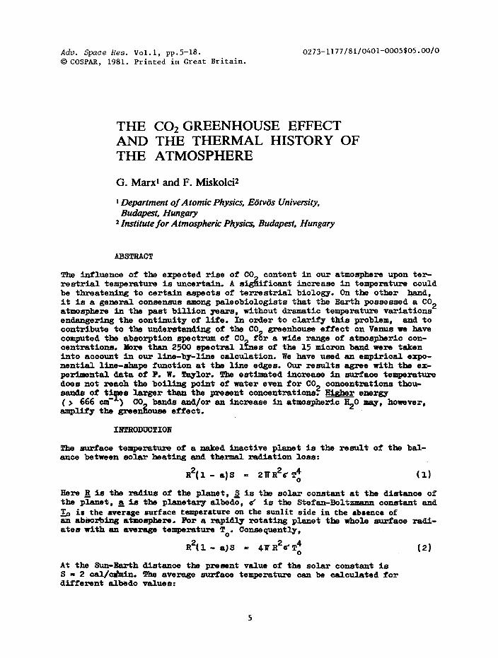
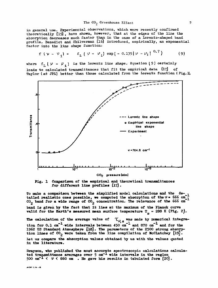
in general use. Experimental observations, which were recently confirmedtheoretically (15], have shown, however, that at the edges of the line theabsorption decreasesmuch faster than in the case of a Lorentz—shaped bandprofile. Benedict and. Shilverman [16] introduced, empirically, an exponentialfactor into the line shapefunction:

f - “I) = ~L ( V - V1) exp( - 0.135 - ~ 0.7) (9)

where ~L ( — ~ is the Lorentz line shape. Equation (9) certainly

leads to calculated transmittances that fit the empirical data [17) of

Taylor (at JPL) better than those calculated from the Lorentz function (Pig.2~.

.8

Lorentz line shape

/ o Empirical exponential

E I’ line shapeK/ — Experiment

C _______ ‘J764.6 cm-1

11114 I I I 11)111 t I I ~ i i ItLIl II I I

1 101 1Ol 10~

CO2 pressure jatmi

Fig. 1 Comparison of the empirical and theoretical tr~u,cttn{ttances

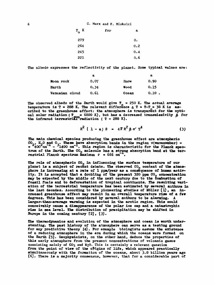
for different line profiles [17).To make a comparison between the simplified model calculations and thetailed realistic ones possible, we computed the absorption of the ~‘ = 666 cm1CO2 band for a wide range of 002 concentration. The’ relevance of the 666 cm

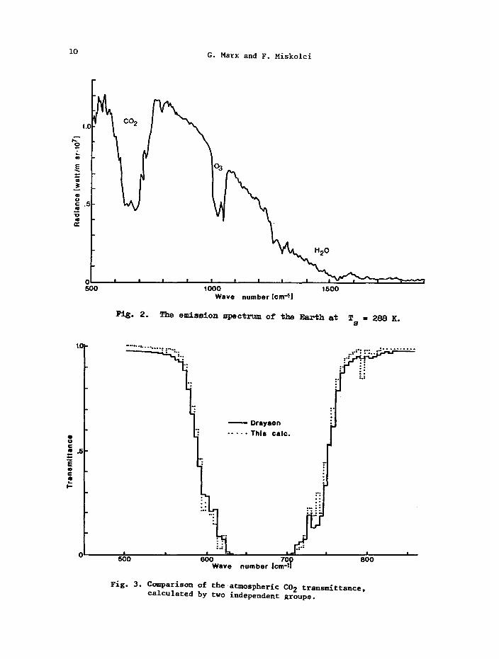
band is given by the fact that it lies at the maximum of the P].ancic curvevalid for the Earth’s measuredmeansurface temperatureT = 288 K (Fig. 2).

The ca].culationof the average value of Z~,~ was made by numerical integra-

tion for O.). cm .~wideintervals between450 cm and 870 cm and for the1962 US StandardAtmosphere [18). The parametersof the 2500 strong absorp-tion lines of 002 were taken from the line compilation of McClatchey [193.

Let us compare the absorption values obtained by us with the values quotedin the literature.

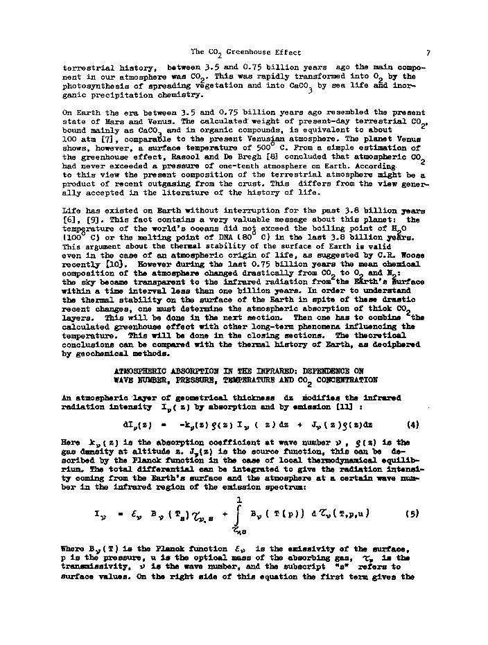
Drayson, who published the most accurate spectroscopic calculations calcula-ted treml’m(ttance averages over 5 cm~wide intervals in the region500 ciC

1 ( P < 860 cm • He gavehis results in tabulated form (20].

JASR 1~l4-8


Co2i0

0

o~

0C .5

‘00

H20

I I t I I I I I I

500 1000 1500Wave number tcnr

1J

Pig. 2. The emission spectrum of the Earth at T5 288 K.

1.0 : r...

— DraysonThis caic.

CUC

CCCI-

C 640 - 700 800Wave number (cm-li

Fig. 3. Comparison of the atmospheric co2 transmittance,calculated by two independent groups.


Figure 3 offers a comparison of his calculated transmittancea with those ob-tained by us in the present study. Though there are significant differencesat specific wave numbers, the integrated absorptions A are in good agreement(Table 1).

TABLE 1 Integrated Absorption Values A as a Function of

Atmospheric Preasure

Atmospheric Pressure Drayson Present authors

1 nib 1.45 cm1 1.93 cm~

10 nib 9.10 cm~ 9.90 cm~

100 nib 52.48 cm~ 57.66 cm~

1000 nib 161.75 cm1 - -- 157.20

The slight differences may have several possible reasons: 1) The presentcalculation used 320 ppm by volume compared with 310 ppm used by Draysori;the influence of this difference on the calculation is small. 2) The lineparameters used were not c~ompletelyidentical. 3) Drayson divided the atmos-phere into 34 homogeneouslayers, the present calculation used 16 layers.4) At the line edgesthe shape function used by Drayson was rather differentfrom the one used by us.

In spite of these differences one may regard the general agreement of the twocalculations as an indication of the correctness of this method for the deter-mination of the integrated absorptions A and‘L Therefore we continued thecalculation to compute the dependence of A andI on CO

2 concentration. Tiealso eri~ininedthe influence of variations in temperatureand pressure on theabsorption.

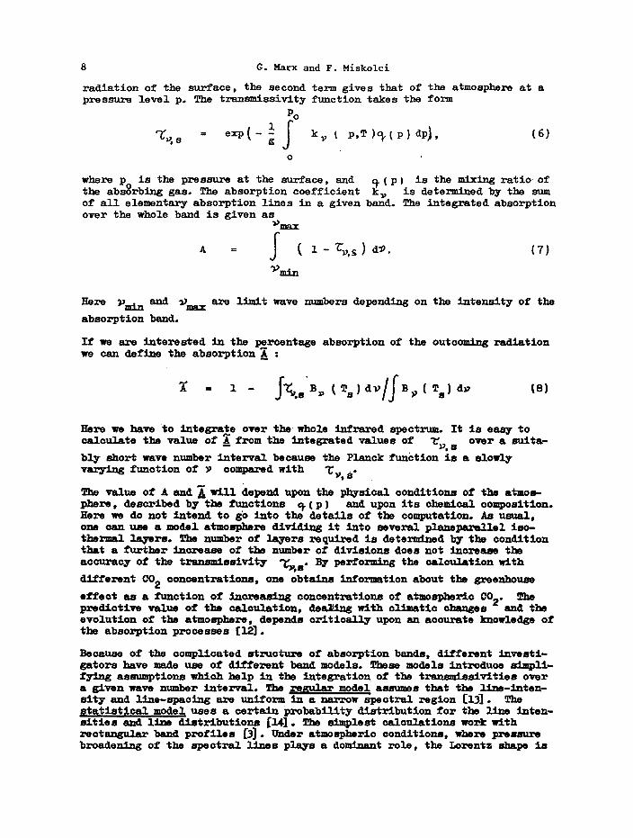
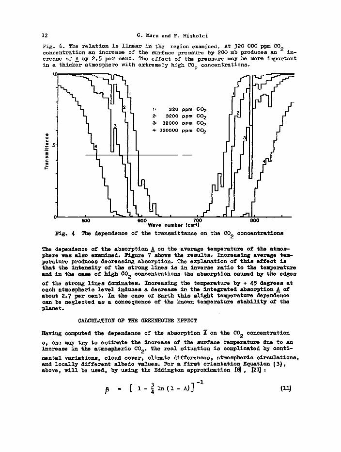
In order to determine the concentration dependence, the present atmospheric002 oonoentration of 320 ppm was increased5-, 10-, 50-, 100- and 1000—fold.

The variation of the tr=’nsmlttance is shown in Fig. 4. The variation of theabsorptions A and A is in Pig. 5. In the case of A the integration limits

were p = 10 cm~and i~ - 2500 cm1. It can be seen from the solid curve of

Fig. 5 that the integrated absorption A depends on the concentration aa apower function. We fitted a power function to the points of A by the leastsquare method:

0.1016A = l56.l3( ~) cm~, (10)

where c is the 002 concentration and c~= 320 ppm is the present 002 level.

The correlation coefficient was larger than 0.99.

Another important question is how the integrated absorption depends on pres-sure and temperature at high 002 concentrations. Higher 002 concentration

will result in an increase of the average molecular weight of the atmosphere,and consequently in an increase of the surface pressure. This effect wasinvestigated oni,y at the thousandfold CO

2 concentration. In this case the

pressure on the Earth’s surface was 1261.0 nib, and the atmosphere consistedof about 30 ~ 002 and 70 % N2. The dependenceof the differential integrated

absorption 4A on the variation of the total surface pressureAP Is shown in


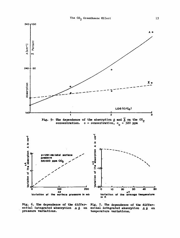
Fig. 6. The relation is linear in the region examined. At 320 000 ppm CO2concentration an Increase of the surface pressure by 200 nib produces an in-crease of A by 2.5 per cent. The effect of the pressure may be more Importantin a thicker atmosphere with extremely high CO, concentrations.

1J~~

~, 12 I l~ 320 ppm CO2 II 1 7 2 3200 ppm CO2 2

3 32000 ppm CO2

.5 \~~I20000 ppm C~J4~/

500 600 700 800Wave number (cm-li

Pig. 4 The dependence of the tr~n~m1ttance on the CO2 concentrations

The dependenceof the absorption A on the average temperature of the atmos-phere was also e~am{,~d.Figure 7 shows the results. Increasing average tem-perature produces decreasing absorption. The explanation of this effect isthat the intensity of the strong lines is in inverse ratio to the temperatureand in the case of high CO2 concentrations the absorption causedby the edges

of the strong lines dominates. Increasing the temperatureby + 45 degreesateach atmospheric level induces a decrease in the integrated absorption A ofabout 2.7 per cent. In the case of Earth this slight temperaturedependencecan be neglected as a consequenceof the known temperaturestability of theplanet.

CALCULATION OP THE GREENHOUSE EFFECT

Having computed the dependence of the absorption I on the CO2 concentration

c, one may try to estimate the increase of the surface temperature due to anincrease in the atmospheric 002. The real situation is complicated by conti-

nental variations, cloud cover, climate differences, atmospheric circulations,and locally different albedo values. For a first orientation Equation (3),above, will be used, by using the Eddington approximation [~, [2]):

p = [ l-~in(l-A)] (11)


340 100

Ao

— a7 ~E ao -I-

< 1<

240 50 o

Xe

~~~--~~0

a —

LOG(CIC0)14C 2 3

Pig. 5. The dependenceof the absorption A andI on the CO2concentration. c = concentration, c0 — 320 ppm

•1•EU CC —

C

p—1261 mbtotal surface .,

pressure320000 ppm CO2 ..

<a aa.

£—

-. -, 00C —2 —

a~ ,a a>1 >-2C

0 100 200 0 tO 20 30 40 50aT

Variation of the surface pressure in mb Variation of the average temperatureIn K

Fig. 6. The dependenceof the differ -Pig. 7. The dependenceof the differ-entia]. integrated absorption A A on ential integrated absorption ~ j~ onpressurevariations, temperaturevariations.

14 The CO2 Greenhouse Effect

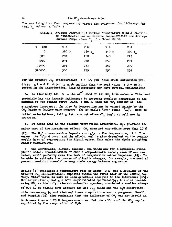
The resulting T surface temperaturevalues are collected for different ini-tial T values in Table 2:

0

TABLE 2 Average Terrestrial Surface TemperatureT as a Functionof Atmospheric Carbon Dioxide Concentration and AverageSurface TemperatureT of a Naked Earth

c ppm TK TK TK TIC0 280 T 260 T 240 P 220 T

0 0 0 0

320 289 268 248 227

3200 291 270 250 229

32000 294 273 252 230

320000 300 279 258 236

For the present CO2 concentration c = 320 ppm this crude estimation pro-.

dicta ~T=8K wbiohismuohsmallerthantherealvalue AT=38K,quoted in the introduction. This discrepancy may have several explanations:

a. We took only the )? — 666 cm~band of the ~°2 into account. This band

certainly has the largeàt influence: it produces complete absorption at themaximum of the Planok curve (Pigs. 3 and 4,1. When the CO2 content of theatmosphere increases, the rise in temperature may be causedmainly by theCO2 bands of higher wave numbers the so called “hot” bands [12]. More de-

tailed calculations, taking into account other 002 bands as well are inprogress.

b. It seems that in the present terrestrial atmosphere,1120 produces the

major part of the greenhouseeffect; CO2 does not contribute more than 10 %(23]. The 1120 concentration depends strongly on the temperature, it influ-ences the cloud cover and the albedo, and is also dependent on the consid-erable heat of evaporation for liquid water. This makesthe whole situationrather complicated.

c. The oontinenta, clouds, seasons, and winds ask for a dynamical atmos-pheric model. Consideration of such a comprehensive model, even if one ex-isted, would probably make the task of computation rather hopeless (24). Tobe able to estimate the course of climatic changes, for example, one must atpresent restrict oneself to very crude energy balance arguments.

loller f 1) predicted a temperature rise of about 2 K for a doubling of thepresent CO2 concentration, expected within the first half of the coming cen-tury. This value is more or less generally accepted in the literature 125].Our calculations, using a more sophisticated apectroscopy, but also consid-ering 002 as the only relevant molecular species, concluded a smaller change

of 0.5 K, By taking into account the hot 002 bandsand the H2O absorption,

this number may be modified and these computations are in progress. Newelland Dopplik (23] also emphasizethat the influence of CO2 can not result in

muchmore than a 0.25 K temperature rise. But the effect of the CO2 may beamplified by the evaporation of 1120.


The increase in the concentration of the atmospheric CO2 is an empirical fact

of the past decades, but this has not beenassociatedwith an observedglobalrise of temperature [261. The explanation is not clear. One possibility isthat smog increases the albedo of the Earth, which works in the direction ofa temperaturefall, and the two independent phenomenamay compensate eachother. A network of chemical and biochemical reactions may produce even anegative greenhouse effect [27]. The present trends of climatic variation area subject of debate that careful measurements and good theory could domuch to temper.

GEOCBEIAICAL CONSIDERATIONS

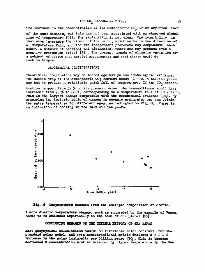
Theoretical conclusions may be tested against paleoclimatologica]. evidence.The sudden drop of the atmospheric 002 content about ]. — 0.75 billion yearsago had to produce a relatively quick fall of temperature. If the CO2 concen-

tration dropped from 32 % to its present value, the tri~namittance would haveincreased from 75 % to 88 %, corresponding to a temperature fall of 10 — 12 K.This is the largest change compatible with the geochemicalevidence 128]. Bymeasuring the isotopic ratio of oxygen in oceanic sediments, one can obtainthe water temperaturefor different ages, as indicated on Pig. 8. There isan indication of cooling in the last billion years.

K

350 e e e

.300

0

Ew

25C-4 -3 -2 -1 0Time (billion year)

Fig. 8 Temperaturesdeduced from the isotopic composition of cherts.

A more drastic temperature change, such as suggestedby the example of Venus,seemsto be excluded empirioally in the case of our planet (29].

CONCLUDING REMARKS ON THE THERMAL HISTORY OF THE EARTH

Most geophysical calculations assumean invariable solar constant. But thestandard solar model, and evennonconventiona].models indicate a 5 ±1increase in the solar luminosity per billion years DO]. This is becausedecreasedH concentrationmust be balancedby higher temperature in the Sun.


This means, that going back in time, the temperature of the Earth’s surfacemust be decreasedby 4 K each billion years taking into account the smallersolar luminosity. This helps to moderate the greenhouseeffect. The time de-pendence of the two effects are, however, completely different: the solar re-actor warms up smoothly; the sudden disappearance of the CO2 shield, on the

other hand, results in a rapid cooling in the last one billion years.

Another phenomenon,which in principle might have played an important role inthe past, was the heat produced by terrestrial radioactivity. For a sourceproducing an average power W(t) per unit volume of the planetary interior,Equation (3) must be modified to

R~W(t) + •ii~R2( 1 — a) S = 47T R26’~ P4 (12)

The value of Vi(t) is not known exactly,40but it can be estimated. For sim-

plicity, let us restrict ourselves to K decay. The present concentration40 . 40

is about one gram K per ton of crustal material. If the K were distrib-uted uniformly within the Earth, the energy producedby its radioactivitywould correspond to 0.2 per cent of the solar constant. But this is certainlyan overestimation: the light elements are concentrated in the surface layers

of the planet. The life time of40K is 1.28 billion years,

40 so that at thetime of the Earth’s formation the heat production from K and from U andTh did not exceed half a per cent of the solar heating. The contribution ofthe radioelements thus did not have a large influence on the thermal historyof the Earth in the last 3.1 billion years, and only radioelements with life-times considerably shorter than one billion years heated up the planet in thefirst billion years of its existence; but these nuclei quickly disappeared.In stmmiary, though U(t) might be significant at the beginning, becauseit hada half lifetime smaller than one billion years, it becamenegligible afterthe formation of the planet.

Another early energy source for the Earth was tidal friction. The Moon wasmuch nearer in the early era of the Solar Systemand the Barth rotatedfaster. It is rather bard to estimate this effect [31], but at best it couldhave had a si-g~iificant contribution only in the first billion years; later itbecamenegligible.

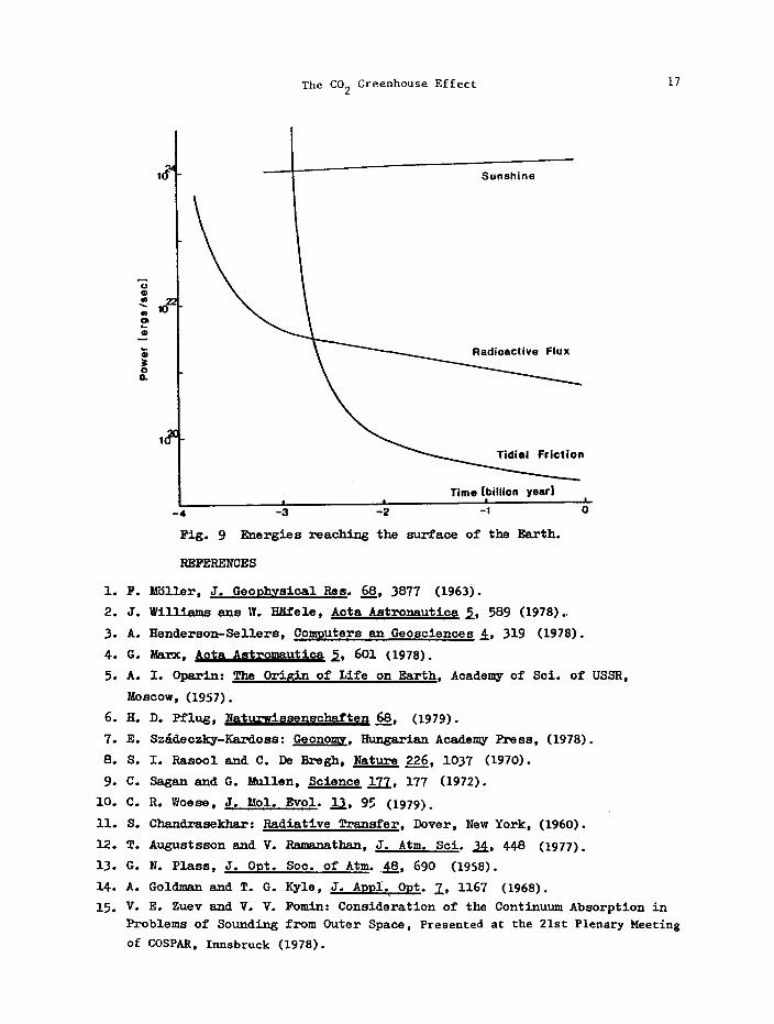
In Fig. 9. the time dependence of these various factors is summarized. Thepower reaching the surface of the Earth did not decrease in the last threebillion years. The observedslight temperaturedecrease can be expi-ainedonly by a decreasing CO2 content.

The thermal stability of Earth -- an ocean temperaturebetween270 K and350 K in the past 3.8 billion years -— still needs a more convincing expla-nation. The different large-scale effects have completely different time de-pendencies, so the cancellation is still surprising. Lovelock and Margulis[32) assumedthat the biological ecosystem called Earth is a aelfregulatingorganism, which takes care of itself, even by stabilizing the climate. Thisidea is far from being an elaborate quantitative theory, but let us remarkthat the only way by which the terrestrial life can influence atmosphereisby changing its 002 concentration.

If the mankind is interested in its past and in its future, one has to un-derstand the working of this greenhouse in every detail.


Ii Sunshine

C

~ z~1o

0

Radioactive Flux00.

Tidiel Friction

Time (billion year)

-4 -3 —2 -1

Fig. 9 Energies reaching the surface of the Earth.

REPERENCES

1. F. M~5ller, J. GeophysicalRca. 68, 3877 (1963).

2. J. Williams ens W. Hä.fele, Acta Astronautica ~, 589 (1978).

3. A. Henderson—Sellers, Computers an Geosciences j, 319 (1978).

4. 0. Marx, Acta Astromautica ~, 601 (1978).

5. A. I. Oparin: The Origin of Life on Earth, Academy of Sci. of USSR,

Moscow, (1957).

6. H. D. Pflug, Naturwissenschaften ~, (1979).

7. B. Szádeczky—Kardoss: Geonomy, HungarianAcademy Press, (1978).

8. 5. I. Rasool and. C. De Bregh, Nature 226, 1037 (1970).

9. C. Sagan and 0. Mullen, Science ~fl, 177 (1972).

10. C. R. Woese, J. Mol. Evol. ~, 95 (1979).

11. S. Chandrasekhar: Radiative Transfer, Dover, New York, (1960).

12. P. Augustason and V. Ramanathan,J. Atm. Sci. ~, 448 (1977).

13. 0. N. Place, J. Opt. Soc. of Atm. ~, 690 (1958).

14. A. Goldman and T. 0. Kyle, J. AppI. Opt. 1~1167 (1968).

15. V. E. Zuev and V. V. Fomin: Consideration of the Continuum Absorption inProblems of Sounding from Outer Space, Presented at the 21st Plenary Meeting

of COSPAR, Innsbruck (1978).


16. W. S. Benedict and S. Shilvermaim, Line Shapes in the Infrared. Paper

given at meeting of Atm. Phys. Soc. 1954.

17. P. W. Taylor, Private communication 1980.

18. U. S. Standard Atmosphere, U. S. Government printing office, Washington

D. C., 278 pp. 1962

19. H. A. McClatchey et al. APCRL — PR — 73 — 0096 1973

20. S. R. Drayson, Univ. Michigan Tecbn. Rep. 05863 — 3 — T, 52 1964.

21. A. E. Ringwood, Advances in Earth Science, 1964.

22. H. D. Holland, A Model for the Evolution of the Earth’s Atmosphere, in:

Petrologic Studies, p. 447, 1962.

23. R. E. Newell and T. G. Dopplick, J. Appi. Met. 18, 822 (1979).

24. J. Smagorinsky, Weather and Climate Modification, J. Wiley and Sons,

New York, 1974, p. 60.

25. S. Manabe and R. P. Wetherald, J. Atm. Sd. ~, 3 (1975).

26. R. W. Stewart, Atmosphere — Ocean].6, 367 (1978).

27. R. Siemerling at the Aspen Seminaron “On the consequencesof a

hypothetical world climate scenario due to increased C02” (1978).

28. S. Epstein and L. P. Knauth, Geochimica and CosmochimicaActa &Q~1095(1976).

29. P. M. L. Wigley et ml., Nature ~ 17 (1980).

30. L J. Newman and H. P. Rood, On the Evolution of the Solar Constant.

Orange Aid Preprint No. 585, California Institute of Technology, Pasadena.

31. H. Turcotte, Icarus ~ 254 (1977).

32. J. Lovelock and L. Margulis, New Scientist ~, 391 (1978).

the co2 greenhouse effect and the thermal history of the atmosphere

Documents