the changing incidence of extremes in worldwide and central england temperatures to the end of the...

THE CHANGING INCIDENCE OF EXTREMES IN WORLDWIDE ANDCENTRAL ENGLAND TEMPERATURES TO THE END OF THE

TWENTIETH CENTURY �

E. B. HORTON, C. K. FOLLAND and D. E. PARKERHadley Centre for Climate Prediction and Research, Met. Office, London Road, Bracknell,

Berkshire RG12 2SY, U.K.

Abstract. Annual and seasonal gridded ocean surface temperature anomalies show an increase inwarm extremes and a decrease in cold extremes since the late 19th century attributable entirely tothe overall warming trend. Over land, however, a reduction in the total incidence of extremes mayreflect improved instrumental exposures. Our estimates of extremes are made by deriving percentilesfrom fits of anomalies on 5◦ latitude × 5◦ longitude resolution to modified 2-parameter gamma dis-tributions. A non-parametric method is used to check the validity of the results. Fields of percentilescreated using this technique can be used to map the distribution of unusual temperature anomaliesacross the globe on any time scale from a month to about a decade, from 1870 onwards. We applya similar technique to assess changes in the incidence of extreme daily Central England temperatureanomalies. The incidence of these extremes, relative to individual monthly average temperatures, hasdeclined.

1. Introduction

The purpose of this paper is to investigate changes in the incidence of extremewarm and cold temperatures over the globe since 1870 on seasonal and annual timescales. We also provide a local perspective using the long daily Central Englandtemperature data set.

The assessment of the return period or percentage likelihood of an event maybe made in a variety of ways. Empirical methods e.g., Chegodayev (1953) andJenkinson (1977) (henceforth CJ), based on ranks of the data, work well for largesample sizes e.g., n > 100 (Appendix A; Folland and Anderson, 2001). Withsmaller samples this method cannot be used to analyse the tails of the distribution(see Appendix A). In small sample situations, analytical distribution curves areoften fitted to the available data: how well these distributions fit can be assessedby a range of objective techniques for assessing goodness of fit (Nicholls andMurray, 1999). When the data themselves are averages of many observations, theCentral Limit theorem indicates that it is likely that a Gaussian fit may be adequate.However, observations of instantaneous meteorological parameters, and totals ofsporadic phenomena such as rainfall, are likely to be highly non-Gaussian and

� The British Crown right to retain a non-exclusive royalty-free license in and to any copyright isacknowledged.

Climatic Change 50: 267–295, 2001.© 2001 Kluwer Academic Publishers. Printed in the Netherlands.

268 E. B. HORTON ET AL.

significantly skewed. In particular, distributions which are physically constrainedto be positive or zero, like rainfall, are likely to be positively skewed. In such cases,gamma or lognormal distributions are likely to provide more skilful fits. Percentilesbased on Gaussian distributions cannot of course account for skewness, whichmakes a positive deviation of a given magnitude either more (positive skewness)or less likely (negative skewness) than a negative deviation of the same magnitude.Thus, Bradley et al. (1987) analysed trends and interannual variations of global andregional precipitation in terms of percentiles based on the gamma distribution.

Other distributions that could have been fitted to the data include the Type I,II or III extreme value distributions (Jenkinson, 1955; Von Storch and Zwiers,1999). These are generally fitted to a series of maximum or minimum events, ratherthan to the whole data sample. For example, for annual temperatures one might fitthe maximum annual temperature in each decade and determine the return period(in decades) for a particular annual temperature to be exceeded. However, for atime series that exhibits a trend (such as the air temperature series over the past150 years) it is clear that the results of such an analysis would be worthless if thewhole period were used, and if a shorter period were chosen to reduce the trend(e.g., 1961–1990) very few data points would be available to use in the analysis.

In this study our aim is to investigate changes in the incidence of extremetemperature anomalies, extending work recently reported by Jones et al. (1999)following the Workshop on Indices and Indicators for Climate Extremes held atAsheville, NC, U.S.A., in 1997. Since temperature anomalies may be positive ornegative, there is no imposed bias towards positive skewness. Nonetheless, tem-perature anomalies sometimes have skewed distributions. In the United Kingdom,daytime maximum temperatures are positively skewed in summer and, to a lesserextent, negatively skewed in winter (Parker et al., 1992). Nighttime minima tendto be slightly negatively skewed throughout the year. Because the daily data areautocorrelated, averaging into months or seasons is not sufficient to entirely removethe skewness: thus, the warmest winter in the 20th century in the Central Englandtemperature series (1988–1989) was 2.4 ◦C above the 1961–1990 average, but 5winters in the 20th century were more than 2.4 ◦C colder than that average (Manley,1974; Parker et al., 1992). Although annual anomalies are less likely to be skewed,owing to the longer-period averaging, this is not always the case: for example,annual sea surface temperature anomalies in the eastern equatorial Pacific areaaffected by El Niño events are positively skewed, partly owing to the persistence ofthe events, as illustrated in Section 6.2 below. So we have chosen to base most ofour analyses of temperature anomalies on the gamma distribution, irrespective oftimescale, to give a uniformly rigorous and systematic approach. We show that thisapproach is adequate for the data analysed here. To make this approach applicableto negatively skewed data, we invert the anomalies to provide a positively skeweddistribution to which can be fitted to the gamma function. We recognize that thegamma distribution tends to the Gaussian distribution when the skewness is small,

THE CHANGING INCIDENCE OF EXTREMES 269

so in this sense the Gamma distribution provides a unified framework to cover thefull range of skewness.

Our data base and processing are described in Section 2. Section 3 and Ap-pendix A briefly review the empirical method of estimating percentiles. We thenpresent the 2-parameter gamma distribution (Section 4 and Appendix B) and ourmodification to it to enable negative anomalies and negative skewness in the data tobe allowed for (Section 5 and Appendix C). Section 6 examines the goodness of fitof the modified gamma distributions to the data, and in Section 7 and Appendix Dwe describe the derivation of the percentiles. Our analyses of worldwide annualsurface temperature anomalies is in Section 8, and Central England temperature isanalysed in Section 9. Conclusions are drawn in Section 10.

2. Data

To study the behaviour of temperature extremes worldwide, we used new 5◦ lat-itude by 5◦ longitude gridded monthly mean blended land air and sea surfacetemperatures (Jones et al., 2001). These data are a further development of the landair temperatures of Jones (1994) and the sea surface temperatures of Parker et al.(1995), both of which are expressed as anomalies relative to a 1961–1990 clima-tology. They have been adjusted to remove spurious changes in variance caused byhistorical variations in the amounts of data within grid boxes and so are much moresuitable for the analysis of changing extremes. The monthly anomalies were aver-aged into seasonal and annual anomalies. Three-month ‘seasonal’ anomalies werecalculated provided at least one monthly anomaly was available. Annual anomalieswere only calculated if all four seasonal values were available. We used the 30annual fields for 1961–1990 to calculate the climatology of annual percentiles.We chose this limited base period partly because of the consistently better datacoverage than previously available and partly because other ongoing efforts in theanalysis of changing extremes are likely to use this base period (e.g., Manton etal., 2001). Furthermore, the overall change of temperature in many parts of theworld was relatively small during 1961–1990, and this is also the reference periodused in the recent Assessments of the Intergovernmental Panel on Climate Change.Nonetheless, these annual fields were not complete, so percentile anomalies werecalculated only in grid boxes with more than 20 anomalies out of the maximum of30. The percentiles chosen for analysis were 2%, 5%, 10%, 20%, 30%, 40%, 50%,60%, 70%, 80%, 90%, 95%, 98%. Data since the late 19th century from the samedata bases were then used to assess changes in the incidence of these percentiles. Inthis paper we mainly present results for the 10th and 90th percentiles. We choosethese percentiles as they are not so near the extremes of the distribution that majorchanges cannot be reliably estimated. This could happen if, for example, valuesless than the 5th percentile were almost never observed in a warming climate.


For analyses of seasonal or monthly values we again required at least 20 con-stituent seasons or months. For daily Central England temperature, we used anupdate of the complete series developed by Parker et al. (1992). All data end in1999.

3. Empirical Method

In each gridbox, temperature anomalies at each of the chosen percentiles wereidentified using the CJ method. This non-parametric method provides an estimateof the most probable value of the percentile that is associated with each value in aset of ranked data. A brief description appears in Appendix A and a full analysisfrom first principles is being prepared (Folland and Anderson, 2001). Missing datawere only accounted for in that, as above, only boxes with more than 20 annualanomalies were used. The CJ percentiles were compared with those found fromfitting the gamma distributions to the anomalies.

4. The 2-Parameter Gamma Distribution

There is no perfect method for fitting a curve to a set of data with an arbitrary but,we assume here, a unimodal distribution. The gamma distribution is, however, veryflexible and can accommodate major variations in distribution shape and skewness.

The general form of the 2-parameter gamma density function is given below:

f (x) = 1

ba(a)e−x/bxa−1 a > 0 , (1)

where x is the variable being studied and (a) = (a − 1)! is the complete gammafunction. The 2 parameter gamma distribution is fully described by the parametersa and b. Appendix B gives details of the derivation of a and b. Note that thegamma distribution is positive definite: see Section 5 for the treatment of negativeanomalies.

The values of a and b control the shape and scale of the gamma curve respec-tively (Figure 1) with a positive coefficient of skewness, G = 2a−1/2 (Haktanir,1991). Distributions with 0 < a ≤ 1.0 are asymptotic, while distributions witha > 1.0 have minima at x = 0.

As the value of a increases, both the skewness and kurtosis decrease, and thedistribution becomes more Gaussian. Ropelewski and Jalickee (1983) state that forpractical purposes the difference between the gamma and normal distributions isnegligible for values of a > 50. With a = 51, the coefficient of skewness, G, isonly 0.28.

We used the maximum likelihood method to estimate a (Appendix B). Thismethod is like CJ in that it estimates the most probable percentile value corre-sponding to specific values in the distribution (Thom, 1957; Essenwanger, 1985).


Figure 1. Gamma frequency distribution curves with (top) b = 1 and various values of parameter a;and (bottom) a = 2 and various values of parameter b.

However, for small samples, the maximum likelihood method is biased (Essen-wanger, 1985), so we used a correction recommended by Bridges and Haan (1972)and given in Essenwanger (1985) (Appendix B). The scale parameter, b, is thenfound from the relationship b = µ/a where µ is the mean of the sample.

5. The Modified 2-Parameter Gamma Distribution

Gamma distributions are positively skewed and positive definite. To fit them totemperature anomalies, we first transformed the anomalies to make them positivelyskewed with no negative values. We did this by reversing the sign of the anomalies


if the original data were negatively skewed, then adding a location parameter c, andcalculating a related parameter q such that the distribution was defined betweenq(> 0) < x < ∞. Details of the transformations are given in Appendix C.

The transformations do not affect the kurtosis or the magnitudes of the coeffi-cient of skewness. However, the transformations do affect the estimates of a and b,and thus the skewness of the fitted distributions. We tune the skewness of the fitteddistribution to be as similar as possible to that of the observed distribution by aniterative choice of c. A gamma distribution is fitted in this way to the transformedtemperature anomaly distribution in each grid box. Each grid box and calendarperiod (e.g., monthly) temperature anomaly distribution will have different valuesof a and b.

6. Testing for Goodness of Fit of Worldwide 5◦ Latitude by 5◦ LongitudeGridded Data

6.1. CUMULATIVE FREQUENCY DISTRIBUTION PLOTS

A visual check was made by plotting the cumulative frequency distribution of theobserved and fitted annual and monthly data. Cumulative frequency distributionsfor four chosen gridboxes are given in Figure 2 and discussed later.

6.2. KOLMOGOROV–SMIRNOV TESTS OF OBSERVED AND FITTED

DISTRIBUTIONS

A Kolmogorov–Smirnov test (Siegel and Castellan, 1988) was performed on thetemperature anomalies in each grid box to test the null hypothesis that the fittedmodified two-parameter gamma distribution and observed data (after the trans-formation described in Section 5) were from the same population. The test wasthen repeated using a Gaussian distribution to determine whether the gamma fitprovided a significant improvement over simply fitting the data to Gaussian dis-tributions. Both tests were applied to annual and monthly data. Because tests ondistributions are generally poor when the samples are small we used the period1950–1999, and required at least 35 values in each gridbox sample. All the sta-tistical tests rely on the assumption that the sample data are independent (Siegeland Castellan, 1988), but annual and to a lesser extent, specific calendar monthly(i.e., all January) temperature anomalies are not independent. So the critical valueused in the Kolmogorov–Smirnov test was determined using the equivalent num-ber of independent values (Waldo Lewis and McIntosh, 1952) rather than thetotal sample size. We used the sample data to estimate the parameters for theGaussian and Gamma distributions. This ensures that the Kolmogorov–Smirnovtest is conservative (Siegel and Castellan, 1988).

None of the 1645 globally distributed annual samples was rejected by theKolmogorov–Smirnov test at the 10% significance level when tested against the


Figure 2. Examples of fitting gamma and Gaussian distributions to December temperature anomalies.(a) and (b) Two samples where the gamma cumulative frequency distribution is an improvement overthe Gaussian (El Niño area and Central Asia). (c) An example of a distribution that is slightly betterfitted by the Gaussian distribution. (Southern Ocean). (d) An example of a distribution that is equallywell fitted by gamma and Gaussian cumulative frequency distributions (Indian Ocean, southwest ofAustralia).

fitted gamma distributions but 4% were rejected when tested against the Gaussiandistribution. For the monthly data, 1% of gridbox samples were rejected whentested against the gamma distributions, and 3–10% (depending on the calendarmonth) were rejected when tested against the Gaussian distribution. Additionally,for the monthly data there was a seasonal pattern, with more samples rejectedas being Gaussian during November to March than during the rest of the year.As expected, most of the non-Gaussian distributions are in the northern interiors


of North America and Eurasia during winter. Figure 2 compares the cumulativefrequency distributions for December values for a selection of grid boxes withtheir fitted gamma and Gaussian distributions. Figures 2a,b show the cumulativefrequency distributions for boxes in the El Niño area (2.5◦ S, 82.5◦ W) and CentralAsia (42.5◦ N, 97.5◦ E), for which the gamma distribution is clearly an improve-ment over the Gaussian. The data in these samples have skewness of 1.85 and–1.24 respectively. Figure 2c is an example of one of the few gridboxes in whichthe Gaussian distribution would have been a better fit than the gamma distribution,although neither fits the observations well. This sample comes from the South-ern Ocean (57.5◦ S, 77.5◦ E) and the skewness of 2.28 is heavily influenced by asingle (possibly spurious) large positive anomaly. Figure 2d shows the cumulativefrequency distribution for a gridbox that both the gamma and Gaussian distribu-tions fit well, just off the southwest coast of Australia (37.5◦ S, 112.5◦ E). Here theskewness is only 0.18.

Figure 3 shows the pattern of positive and negative skewness for annual tem-perature anomalies across the globe, with gridboxes with absolute skewness above0.28 highlighted, for example in the eastern equatorial Pacific. Of the 1645 anom-aly samples, 720 have skewness >0.28, i.e., a < 50. This is slightly less thanhalf of the total number of samples. The gamma fit to the annual data will be anominal improvement over the Gaussian in these cases (Section 4). A similar ratioof skew to Gaussian gridboxes, defined this way, is found in each of the monthlytemperature anomaly samples. However, as expected, there are more examples ofextreme skewness in the monthly than in the annual data (Section 7).

6.3. DISCUSSION

The nature of temperature anomalies is such that it is probably impossible to ac-curately fit one type of distribution curve to the data in all of the gridboxes. Thegamma distribution was chosen because of its flexibility in providing mostly goodfits to data on all time scales from daily to annual. Note that the use of the newJones et al. (2001) data has had a marked effect on the skewness of the monthlydata which has been reduced compared to an updated combination of the Jones(1994) and the Parker et al. (1995) data.

7. Calculation of Anomalies at the Chosen Percentiles

Once the shape of the distribution has been determined for each box, by calculationof the parameters a, b and c, the percentiles of the gamma distribution must betransformed back to degrees Celsius.

We need to find the value z(p) such that a value taken at random from thetransformed distribution has a specified probability p of taking a value less thanz(p). We used the Wilson–Hilferty approximation (Ropelewski and Jalickee, 1983)


Figure 3. Skewness of annual temperature anomalies, 1961–1990. Gridboxes with absolute skewnessabove 0.28 are highlighted.

to estimate z(p). This approximation is an adaptation of a more accurate algorithmdesigned to calculate the percentiles of the Gaussian distribution, and is widelyused in flood frequency analysis (Haktanir, 1991). Thus once a, b and c have beendetermined for the distribution, then the values at each of the chosen percentilescan be found. Details are in Appendix D.

Haktanir (1991) established that for most practical purposes the Wilson–Hilferty approximation is sufficiently accurate for distributions with skewness G

in the range −1 < G < 1. This includes most of the temperature anomaly distrib-utions analysed here. The Wilson–Hilferty approximation becomes more accurateas the data become less skewed because it is based on the Gaussian distribution.The most skewed annual distribution in our data had a skewness coefficient of1.0, with a = 3.3 and b = 0.46. The most skewed monthly distribution had askewness coefficient of 3.59, with a = 1.255 and b = 1.161. Tests based ontabulations by Haktanir (1991) showed that the Wilson–Hilferty approximationyielded a maximum error of 0.053 in z(p) for G = 3.0, giving a temperature errorof bz(p) = 0.06 ◦C for the most skewed monthly distribution. For the annual data,the maximum error was 0.006 ◦C. Since temperature anomalies are only accurate tothe first decimal place, the Wilson–Hilferty approximation is sufficiently accuratefor any likely values of skewness in monthly to annual temperature data on a 5◦ ×5◦ grid.


8. Analyses and Results: Worldwide Gridded Data

8.1. ANALYSES OF PARTICULAR YEARS

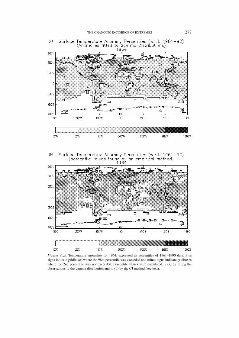
Maps of 5◦ × 5◦ gridded temperature anomalies and corresponding percentileshave been calculated relative to the period 1961–1990 using the CJ and gammamethods for all years in the record. We discuss the maps for annual mean anomaliesfor two years: 1964 (the coldest year in the reference period, see Figures 4a,b) and1998 (the warmest year in the whole record, see Figures 4c,d). We also considerseasonal data for the period December 1997 to February 1998 (Figures 4e,f). Themaps for 1964 (Figures 4a,b) are in good agreement over most of the world. Usingthe gamma distribution method, only isolated locations in the North Atlantic, NorthPacific and Amazonia were as warm as the 90% value. Both methods show thatlarge areas of the subtropical South Atlantic and southwest Indian Ocean, werecolder than the 2% value. The two methods also yield very similar annual mapsfor 1998 (Figures 4c,d), showing anomalous warmth over much of the globe, withthe exception of the central Pacific and northern Eurasia. Temperatures exceededthe 98th percentile in parts of the tropics from the far eastern Pacific throughAfrica to the far western Pacific, as well as in eastern North America, the NorthAtlantic around the Azores, and in eastern Asia. Our preference is for the maxi-mum likelihood gamma method which gives more reliable results for non-normallydistributed data. The very good agreement between the two methods, however, is astrong indication that the gamma method also works well for normally distributeddata.

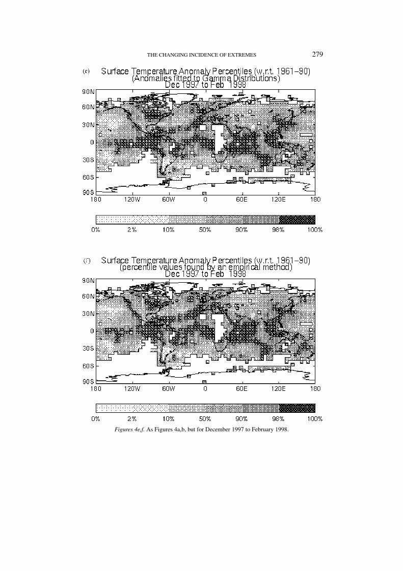
Figures 4e,f compare the gamma and CJ methods for the globally very warmthree month period December 1997–February 1998 (anomaly 0.62 ◦C in the Joneset al. (2001) data set). Anomalies in this season often have greatest skewness overthe Northern Hemisphere extratropics. Nevertheless the two methods again givesimilar results. Thus the gamma method allocates 326 boxes to the 98–100 per-centile category while the CJ method allocates 360 boxes, a difference of about 1%of the total global area. Over the Northern Hemisphere extratropics, the cumulativefractional area allocated to the various percentile ranges is given in Table I. Notethat 15% of the Northern Hemisphere extratropics (north of 30◦ N) has insufficientdata for analysis.

Frequency distribution curves based on the gamma percentiles were createdfor the annual data for 1964 and 1998. These provide a graphic summary of thedifferences in temperature between these years in a way that cannot be captured ina simple average. They are given in Figures 5a,b along with the average cumulativefrequency distribution curve for all years from 1961–1990. When the solid curvelies below the dashed line, more boxes than for the climatological average periodhave anomalies not exceeding the various percentiles, i.e., there is a preponderanceof colder than usual conditions. For example, Figure 5a shows that 73% of boxesin 1964 were colder than their respective 1961–1990 median annual anomalies,


Figures 4a,b. Temperature anomalies for 1964, expressed as percentiles of 1961–1990 data. Plussigns indicate gridboxes where the 98th percentile was exceeded and minus signs indicate gridboxeswhere the 2nd percentile was not exceeded. Percentile values were calculated in (a) by fitting theobservations to the gamma distribution and in (b) by the CJ method (see text).


Figures 4c,d. As Figures 4a,b, but for 1998.


Figures 4e,f. As Figures 4a,b, but for December 1997 to February 1998.


Table I

Fractional area of the Northern Hemisphere extratropics with tem-perature anomalies within each percentile range. Dec. 1997–Feb.1998

Percentile Fractional area of the

Northern Hemisphere extratropics

Gamma CJ

<2% 0.0 0.0

<10% 0.01 0.01

<20% 0.07 0.07

<30% 0.11 0.12

<40% 0.18 0.17

<50% 0.26 0.25

<60% 0.33 0.33

<70% 0.39 0.40

<80% 0.50 0.48

<90% 0.60 0.59

<98% 0.76 0.74

<100% 0.85 0.85

instead of the ‘expected’ 50%. When the solid line lies above the dashed line, fewerboxes have anomalies not exceeding the percentiles, i.e., there is a preponderanceof warmer than usual conditions. Thus, by contrast, in 1998 (Figure 5b), only17% of grid-boxes were colder than the median anomaly (83% were warmer). AKolmogorov–Smirnov test was used to determine whether there was a statisticallysignificant difference between the climatological cumulative distribution and thatfor each of these two years. Not surprisingly, the tests revealed that both the dis-tribution of 5◦ × 5◦ area anomalies in 1964 was significantly colder and that 1998was significantly warmer than the 1961–1990 normal at the 1% significance level.This is likely to be a fairly sensitive method of summarising the state of global (orregional) temperature in individual years.

8.2. TRENDS IN WORLDWIDE INCIDENCE OF ANNUAL AND SEASONAL

TEMPERATURE EXTREMES

Using cumulative frequency distributions like Figure 5, we constructed time-seriesof the fraction of the monitored global area having extreme temperatures (definedrelative to 1961–1990) at the 90% or 10% level on annual, seasonal and monthlytimescales since 1901. Trends in these fractional areas were then estimated usingSen’s non parametric method (Gilbert, 1987). This is based on the median slope


Figure 5. Percentages of anomalies that did not exceed the specified anomaly at each percentileduring (a) 1964; (b) 1998. Each of these cumulative distributions (solid lines) is compared with thatfor all years from 1961 to 1990 (dashed lines).

between all possible pairs of values. We chose this test over simple linear regressionbecause it is less affected by outliers (Lanzante, 1996). The Mann–Kendall ranktest (Gilbert, 1987) was used to determine whether each trend was significant, usinga one-tailed test with H0: no trend and either H1: increasing trend (for fractionalarea with temperatures exceeding the 90th percentile) or H1: decreasing trend (forfractional area with temperatures not exceeding the 10th percentile).

Figure 6a shows time series for 1901–1999 of the fraction of the monitoredglobal area with annual temperature anomalies <10th or >90th percentile as wellas the fraction of global surface area with available gridded data. There was a strongdecline in the proportion of the globe with unusually cold (<10th percentile) con-ditions between 1901 and 1940, from about 40% down to 12%. This is explainedin terms of overall global warming trends in Section 8.3 below. However, between1901 and 1940 the area of data coverage doubled, so the proportional decreasein the area with anomalously low temperatures could have been fortuitously in-


Figure 6a. Fractions of the global data area with annual surface temperatures above the 90th per-centile (solid line) or below the 10th percentile (dotted line). Also shown, in the inset, is the fractionof global surface area with data. The smooth lines are filtered with binomial filters with 21 terms.

fluenced by the increase in total area having data. Nevertheless the proportion ofthe monitored area with unusually warm temperature anomalies increased onlymoderately from 1901 to 1940, indicating that changes in data coverage do notdominate the results. To test this we carried out a frozen grid experiment usingonly gridboxes that had annual temperature anomalies for at least nine years inevery decade. The resulting frozen grid contained 345 gridboxes. The results fromthe ‘frozen grid’ experiment (not shown) were very similar to Figure 6a.

During the Second World War, when data were particularly sparse, the areawith unusually high temperatures reached a peak, which should be regarded withcaution, though this result is in accord with 1941 having been an El Niño year.After 1980 there was a clear rise in the fractional area with temperature anomaliesexceeding the 90th percentile and a corresponding drop in the fractional area withtemperature anomalies lower than the 10th percentile, to very low values (e.g., 0.01in 1995) in some years.

In both the full and frozen grid analyses it is striking how the relative overalldecline in the area of very cold conditions since 1901 is more marked than therelative increase in the area of very warm conditions. However, 1998 stands outas a remarkable year for unusually high temperatures (54% of the global areawarmer than the 90th percentile), almost the same value as the highest percentageof unusually cold values in 1907.


Fig

ure

6b.F

ract

ions

ofgl

obal

data

area

wit

hse

ason

alsu

rfac

ete

mpe

ratu

res

abov

eth

e90

thpe

rcen

tile

(sol

idli

ne)

orbe

low

the

10th

perc

enti

le(d

ashe

dli

ne).

Als

osh

own,

inth

ein

sets

,are

the

frac

tion

sof

glob

alsu

rfac

ear

eaw

ith

data

inea

chse

ason

.The

smoo

thli

nes

are

filt

ered

wit

hbi

nom

ialfi

lter

sw

ith

21te

rms.


Figure 6b shows the fractional global areas with <10th and >90th percentiletemperatures for each three month ‘season’ over 1901–1999. All individual months(not shown) as well as the illustrated seasons show a similar pattern to the annualplots, with large fractional areas of low temperatures at the beginning of the periodand increasing (decreasing) warm (cold) fractional areas after 1980. The relativelygreater overall decline in very cold than the increase in very warm conditions isa little less evident in the December to February data than in the annual data andother seasons.

The annual and seasonal linear trends (estimated using Sen’s method) of theareas warmer than the 90th and cooler than the 10th percentile are all statisticallysignificant at the 95% confidence level according to the Mann–Kendall test. Al-though the trends are, in fact, far from linear (Figure 6), it is clear that both thereduction in very cold areas and the increase in very warm areas are consistentwith the observed warming over the last century.

8.3. INTERPRETATION

The decline in the incidence of extremely low annual temperatures exceeded theincrease in the incidence in extremely high temperatures (Figure 6a). A straight-forward explanation is that the negative average global temperature anomaly at thebeginning of the 20th century was larger than the recent average positive anomaly,relative to the 1961–1990 base period. Thus in the Jones et al. (2001) data theaverage anomaly over 1900–1919 was –0.34 ◦C and over 1980–1999 was 0.22 ◦C.However, the relatively greater decline in cold extremes is a little less evident inthe December to February (Figure 6b) extremes. This is partly because the recentwarmth has been greater in the northern winter (average anomaly 0.29 ◦C over1980–1999).

Both the decline in anomalously cool areas and the increase in anomalouslywarm areas are strongly influenced by the overall global mean warming trend. Toinvestigate the effect of removing this overall trend, we referenced the grid-pointdata for each year to the global average for that year instead of to the grid-pointaverage over the 1961–1990 base period. Thus the global mean anomaly in the newdata is zero in every year. Because land and sea surface temperature anomalies arelikely to come from different statistical populations, we processed land and oceandata separately. The annual-mean global-mean land air temperature (ocean SST)anomaly for a given year was subtracted from the gridded land air temperature(ocean SST) data for that year. We also recalculated the percentiles from 1961–1990 data treated in this way, so as to remove the effects of all interannual andlonger-term variations of the global average over land or sea from the analysis. Theresiduals should provide an assessment of the distribution of extremes relative tothe annual global-average land or oceanic temperature anomaly. If the distributionswere stable, the fraction of area covered by both percentile limits would be close


Figure 7a. Fraction of global land data area with adjusted (see text) annual surface air temperaturesabove the 90th percentile (solid line) or below the 10th percentile (dotted line). Gridbox anomalieswere first adjusted by subtracting the annual globally-averaged land air temperature anomaly in therelevant year. The percentiles were also calculated from 1961–1990 data treated in this way, so as toremove the effects of all interannual and longer-term variations of the global average. The smoothlines are filtered with binomial filters with 21 terms.

to 0.1 in each decade. By definition 1961–1990 as a whole will give 0.1 for both<10th and >90th percentiles.

The results for land (Figure 7a) show that the areal coverage of the 10th and90th percentiles is fairly stable from 1900 to 1945. Thereafter there is a declinein the incidence of both cold and warm extremes until about 1965–1970. Subse-quently the areal coverage of the 90th percentile is relatively unchanged while thecoverage of the 10th percentile increases. The data density did not change greatlyduring 1940–1965, and the overall decline in the incidence of extremes that may beexpected as a result of the increasing density of the network of observing stationswithin gridboxes, reducing the variance of the gridbox anomalies (Jones et al.,1997) has already been accounted for (Jones et al., 2001), so there should not havebeen an artificial change of variance. An alternative explanation for the mid-20thcentury decline is needed. It is too recent to be a recovery from the influence ofearly instrumental exposures, such as Glaisher stands, though thatched sheds usedin the tropics until the mid-20th century may have contributed to excess warmextremes until then (Parker, 1994). So it remains, for the present, unexplained. It ispossible that there has been a real, externally forced change in the spatial varianceof the land temperatures, but to determine this requires further work. The increasein cold extremes since 1990 is probably because subtraction of large positive annual


Figure 7b. Fraction of global ocean data area with adjusted annual sea surface temperatures abovethe 90th percentile (solid line) or below the 10th percentile (dotted line). Gridbox anomalies werefirst adjusted by subtracting the annual globally-averaged sea surface temperature anomaly in therelevant year. The percentiles were also calculated from 1961–1990 data treated in this way. Thesmooth lines are filtered with binomial filters with 21 terms.

global anomalies from worldwide data has generated relative negative extremesin some tropical and subtropical land areas where the variance of temperature issmall. Over most of the land south of 45◦ N the range of temperature between the10th and 90th percentiles is between 1 ◦C and 1.5 ◦C. The average global land airtemperature anomaly over 1990–1999 is about 0.5 ◦C, one-third to a half of thetotal 10–90th percentile range. Hence subtracting the global temperature anomalyresults in an increased number of grid-boxes falling outside the 10th percentile.

By contrast, the oceanic results (Figure 7b) suggest no change in variance of thegridbox anomalies: these have also been adjusted by Jones et al. (2001) to allowfor variations in amounts of data within grid-boxes. Note the increased incidenceof both warm and cold oceanic extremes in 1983 and 1987, recent El Niño years.This arises from the increased spatial variance of sea surface temperatures duringEl Niño and La Niña events, e.g., the cold midlatitude Pacific which accompaniesEl Niño events (Allan et al., 1996). El Niño and La Niña episodes often begin halfway through one year and do not finish at a year end, so it is difficult to determinestatistically whether El Niño/La Niña years contain more extreme anomalies thanother years. However, we used the Troup Southern Oscillation Index (Allan et al.,1991) smoothed using a binomial filter with 21 terms to classify months within ElNiño (smoothed SOI > 10.0) and La Niña (smoothed SOI < –10.0) episodes, andmonthly percentiles calculated from sea surface temperature anomalies that had


Figure 8a. Fraction of days with Central England temperature below the 1961–1990 5th percentile(light line) or above the 1961–1990 95th percentile (heavy line), 1878–1999. The smooth lines arefiltered with binomial filters with 21 terms.

been adjusted by removing global monthly sea surface temperature anomalies, andfound that during 1901–1999, months during El Niños or La Niñas had on averagea 2% increase in the area of oceanic data with anomalies more extreme than the10th or 90th percentiles. A t-test, with degrees of freedom adjusted to accountfor autocorrelation (Waldo Lewis and McIntosh, 1952), showed this result to besignificant at the 5% significance level.

9. Analyses and Results: Daily Central England Temperature

We include an analysis of extremes in daily Central England temperature both todemonstrate the application of our technique to non-Gaussian data and to providenew information on local extremes in one of the longest homogeneous daily datasets available.

Jones et al. (1999) found no long-term change in the incidence of daily CentralEngland temperatures above the 90th percentile, though there was an increase inthe most recent decade. On the other hand, they found more days below the 10thpercentile before 1930 and especially before 1900. Here, using the same smoothedreference annual cycle as Jones et al. (1999) to estimate the anomalies (the daily1961–1990 climatology smoothed by an 11-term binomial filter), we repeat theabove analysis for the 5th and 95th percentiles, defined relative to 1961–1990(Figure 8). Again, the incidence of very cold days is greater than at present before


Figure 8b. As Figure 8a, but percentiles and numbers of extreme days were calculated using dailyanomalies which had been adjusted by subtracting the monthly mean anomaly. The smooth lines arefiltered with binomial filters with 21 terms.

about 1930: there is also a slight deficit of very warm days before about 1910(Figure 8a). If monthly anomalies are first subtracted from all of the data (Fig-ure 8b), the decline in very cold days is reduced but not eliminated, and excess verycold days persist until the 1950s; there is also a slight excess of very warm daysuntil the 1950s. Subtraction of annual anomalies gives similar results (not shown).Consideration of Figure 8b suggests that the within-month variance of daily CentralEngland temperatures (excluding that due to the annual cycle) was enhanced untilthe 1950s, without much change in skewness. In fact, when the variances of CETanomalies in each month before and after 1950 are compared, they have decreasedin all months except December, although an f-test of the variance before and after1950 shows the change to be significant at the 5% significance level in only 4months. So the incidence of very cold (<5th percentile) and very warm (>95thpercentile) days, relative to individual years’ or months’ averages, was in eachcase about 6% (perhaps a little more for very cold days) rather than the expected5%. The data are complete, so data paucity is not an explanation. The replacementof Stonyhurst by the average of Squires Gate and Ringway at the beginning of1959 coincides approximately with the reduction in within-year and within-monthvariance in Figure 8b, but according to Parker et al. (1992), this change did notaffect the variance of the series. So the decline in within-month variability ofdaily Central England temperature is likely to be real. Further investigations, usingdaily data from each of the four seasons separately reveal that most of the extra


unusually cold days relative to the monthly anomalies before the 1950s occurredin September to November.

10. Conclusions

The modified 2-parameter gamma distribution is a promising method of study-ing temperature extremes on a variety of time scales within a common analysisframework. Comparisons with a more restricted non-parametric method based onranks of the data suggests very good agreement where the data are approximatelynormally distributed and the sample size is large enough for the latter to providea reasonable value. The modified 2-parameter gamma distribution allows regionswith unusual temperature anomalies to be mapped (Figure 4).

The reduction, globally, in very cold areas since 1900 is more prominent thanthe increase in very warm areas except in northern winter where the global warm-ing signal in recent decades has been strongest. Compensation for land-specificand ocean-specific global annual average temperature anomalies suggests that theearlier land data had more variance possibly partly owing to poorer instrumental ex-posures (Folland et al., 2001), though more research is needed to ascertain whetherthere has been a real change in spatial variance. The oceanic surface temperatures,by contrast, have self-consistent variance through history (Jones et al., 2001). Anot dissimilar decline in within-year and within-month variability of daily CentralEngland temperature where the data are considered reliable argues towards somereal effects over land.

The strongly historically changing areas of missing data are the main uncer-tainty affecting the global results. Although the frozen grid experiment did notprovide evidence to the contrary, it may still be necessary to carry out MonteCarlo simulations to fully estimate the size of the uncertainty that time-varying datacoverage introduces. However, it will soon be possible to assess this problem usingunbiased globally (nearly) complete datasets that are being developed. Specifically,it may be possible to extend the calculations using globally-complete analyses ofsea surface temperature and land surface air temperature anomalies which havebeen created by reduced-space optimal smoothing (Kaplan et al., 1997; Rayner etal., 2000).

Acknowledgements

This work was supported by the United Kingdom Public Meteorological ServiceResearch Contract. We thank Prof. C. W. Anderson of the University of Sheffield(U.K.) for useful comments and the reviewers whose comments helped us toimprove both the robustness of the method and the clarity of the text.


Appendix A: Empirical or CJ Method of Calculating Percentile Values

Rank a series of N values in ascending order X1X2 . . . XN . The most probablepercentage likelihood that a random value takes a value of less than Xm is

p = m − 0.31

N + 0.38∗ 100 . (A1)

Then the rank m of the value corresponding to a specific chosen probability p is

m = (0.01p(N + 0.38)) + 0.31 . (A2)

Note that the values of m corresponding to chosen percentiles (e.g., 10%) are ingeneral not integers.

For the 30-year base period, with all 30 values present the rank of the 98thpercentile is 30.08. If only 21 values are present (the minimum number of ob-servations allowed in this study) the rank of the 98th percentile is 21.26. In bothcases it is impossible to interpolate above the maximum value in the series, so anapproximation was made to arbitrarily attribute the maximum value in the seriesto the 98th percentile. A similar problem occurs at the bottom of the series, so theminimum value in the series was assigned to the 2nd percentile. Thus the values atthe 2nd percentile are likely to be too high, while those at the 98th percentiles arelikely to be too low.

Jenkinson (pers. comm.) states that this algorithm works well with all underly-ing distributions that are not greatly different from Gaussian. It is sometimes usedin extreme value analysis where each value being analysed is the biggest or smallestin a given year. Other algorithms exist based on different assumptions about howto analyse the underlying distribution of the ranked values, as other choices thanthe most probable values can be made, but the results are not greatly different.

Appendix B: The Two-Parameter Gamma Distribution

The general form of the 2-parameter gamma density function is given below:

f (x) = 1

ba(a)e−x/bxa−1 a > 0 , (B1)

where x is the variable being studied, and (a) = (a − 1)! is the complete gammafunction.

This gamma distribution is fully described by the two parameters a and b. Thesecan be estimated as a′ and b′ most simply using the method of moments:

a′ = µ2/σ 2 b′ = σ 2/µ . (B2)

where µ = mean of the sample and σ = standard deviation of the sample (Walpoleand Myers, 1978).


The frequency distribution curve is positive definite. Changing the values of a

and b changes the shape and scale of the gamma curve (Figure 1). Parameter a has astrong influence on the shape of the curve, because, for example, a small value of a

means that µ is small (compared with σ ), causing a sharp peak in the curve becauseit is constrained to be positive. Parameter b has a stronger influence on the widthof the curve via σ . The distribution is always positively skewed, with a coefficientof skewness, G = 2a−1/2 (Haktanir, 1991). As the value of a increases, both theskewness and kurtosis decrease, and the distribution becomes more Gaussian.

For highly skewed distributions, with low values of a, the method of moments(Equation (B2)) becomes less reliable because it does not use all of the informationgiven in the sample (Haan, 1977). This problem becomes significant when thevalue of a is less than 10 (Haan, 1977). Therefore we choose a maximum likelihoodmethod to estimate the parameters of the gamma distribution, irrespective of thevalue of a. However, for small samples such as we have, the maximum likelihoodmethod also suffers from bias (Essenwanger, 1985). We have used the methodssuggested by Essenwanger to improve the accuracy of the estimate. The maximumlikelihood estimate of a is calculated from the following:

aT = (1 +√1 + 4A/3)/4A (B3a)

A = ln µ − 1

N� ln xi , (B3b)

where aT = maximum likelihood estimate of a; xi = ith temperature anomaly;µ = sample mean; N = sample size.

The correction is

a = aT

(N − 3)

N. (B3c)

The scale parameter, b, is then found from b = µ/a.

Appendix C: The Modified Two-Parameter Gamma Distribution

We modified the data by reversing the sign if they were negatively skewed, andadding a location parameter c, using one of the following equations:

For data with positive skewness:

zi = xi + c (C1a)

with

c = q + | min(x)| . (C1b)

For data with negative skewness:

zi = c − xi (C2a)


with

c = q + | max(x)| , (C2b)

where min(x) and max(x) are the minimum and maximum values in the seriesin 1961–1990 respectively and q is an arbitrary number, discussed below. Thekurtoses of the distributions x and z are unchanged by either of the above trans-formations. The magnitude of the coefficient of skewness is also unchanged, butin Equations (C2a,b) the sign of the skewness has been changed from negative topositive.

It is now possible, by arbitrarily assigning a value to q, to calculate a and b andso fit a gamma distribution to each transformed distribution. The variance of thetransformed distribution z is the same as that of x, and the mean of z is c ± µx .

In most cases there is little difference between a calculated using the maximumlikelihood method and a′ calculated from the method of moments. a′ = µ2/σ 2 sothat with σ 2

z independent of the value of c and µz = c ± µx , a is proportional to(c±µx)

2. The value of c depends on that assigned to q, so q, through a, controls theshape of the fitted gamma distribution. Increasing q causes the fitted distributionto become less skewed. To ensure that the skewness of the fitted distribution is assimilar as possible to that of the observed distribution, an iterative method was usedto determine the best fit value of q. A first guess minimum value was q = 0.5. Theparameters a and b, and the skewness of the fitted distribution were then calculated.q was then increased repeatedly by 0.1 until the difference between the observedand fitted skewness reached a minimum, whereupon the value of q used was thatwhich gave the closest fit to the skewness. If the value calculated for a exceeded50, the distribution was not significantly different from the Gaussian (Ropelewskiand Jalickee, 1983), so q was assigned the value used in the previous iteration.

Appendix D: Determining the Temperature Anomalies at a SpecificPercentile

We need to find the value z(p) corresponding to a specified probability p thata random value from the distribution takes a value less than z(p). We used theWilson–Hilferty approximation (Ropelewski and Jalickee, 1983):

z(p) = a

(1 − 1

9a+ X(p)

(1

9a

)1/2)3

, (D1)

where X(p) is the value of the Gaussian distribution function at percentile p, and a

is the shape parameter defining the gamma distribution function.Here z is measured in the transformed gamma coordinates and the parameter b

is assumed to be 1.


Fig

ure

D1.

The

infl

uenc

eof

bon

the

valu

eof

the

tran

sfor

med

gam

ma

coor

dina

tez (

p∗ )

=bz (

p)

corr

espo

ndin

gto

apa

rtic

ular

perc

entil

e.T

hele

ftan

dri

ght

hand

grap

hsar

eid

enti

cal,

but

the

absc

issa

has

been

mar

ked

inpe

rcen

tile

poin

tson

the

left

grap

han

das

actu

alva

lues

ofz (

p∗ )

onth

eri

ght.

The

top

grap

hsha

veb

=1.

5,th

ebo

ttom

grap

hsha

veb

=2.

Ara

ndom

valu

eha

s2%

chan

ceof

bein

gin

the

shad

edre

gion

.


In this way, once a and b have been determined for the distribution, then thevalues at each of the chosen percentiles can be found. For distributions where b =1,the values of z(p) returned must be multiplied by the scale parameter b before beingused in the transformation back into anomalies in ◦C (Figure D1). This is becauseµ = a′b′. The full transformations are as follows:

When the skewness of the original distribution is positive:

x(p) = b · z(p) − c . (D2a)

When the skewness of the original distribution is negative:

x(p) = c − b · z(p) , (D2b)

where z(p) = the value corresponding to the pth percentile; x(p) = the temperatureanomaly in ◦C at the pth percentile.

References

Allan, R, Lindesay, J., and Parker, D. E.: 1996, El Niño Southern Oscillation and Climatic Variability(Atlas), CSIRO Publishing, p. 416.

Allan, R. J., Nicholls, N., Jones, P. D., and Butterworth, I. J.: 1991, ‘A Further Extension of theTahiti-Darwin SOI, Early ENSO Events and Darwin Pressure’, J. Climate 4, 743–749.

Bradley, R. S., Diaz, H. F., Eischeid, J. K., Jones, P. D., Kelly, P. M., and Goodess, C. M.: 1987,‘Precipitation Fluctuations over Northern Hemisphere Land Areas since the Mid-19th Century’,Science 237, 171–175.

Bridges, T. C. and Haan, C. T.: 1972, ‘Reliability of Precipitation Probabilities Estimated from theGamma Distribution’, Mon. Wea. Rev. 100, 607–611.

Chegodayev, N. N.: 1953, Computation of Runoff on Small Catchments, Transzhedorizdat (inRussian).

Essenwanger, O. M.: 1985, World Survey of Climatology: General Survey of Climatology, Vol.1B: Elements of Statistical Analysis, H. E. Landsberg (ed.), Elsevier Science Publishers B.V.,Amsterdam, p. 424.

Folland, C. K. and Anderson C. W.: 2001, ‘Estimating Extremes from Ranked Data Using a Non-Parametric Method’, J. Climate (to be submitted).

Folland, C. K., Rayner, N. A., Brown, S. J., Smith, T. M., Shen, S. S. P., Parker, D. E., Macadam, I.,Jones, P. D., Jones, R. N., Nicholls N., and Sexton, D. M. H.: 2001, ‘Global Temperature Changeand its Uncertainties since 1861’, Geophys. Res. Lett., in press.

Gilbert, R. O.: 1987, Statistical Methods for Environmental Pollution Monitoring, Van NostrandReinhold Company, New York, p. 384.

Haan, C. T.: 1977, Statistical Methods in Hydrology, Iowa State University Press, Ames, IA, p. 378.Haktanir, T.: 1991, ‘Practical Computation of Gamma Frequency Factors’, Hydrol. Sci. J. 36, 599–

610.Harter, H. L.: 1976, ‘New Tables for Percentage Points of the Pearson Type III Distribution’,

Technical Release 38, Central Technical Unit, U.S. Soil Conservation Service, USGS, U.S.A.Jenkinson, A. F.: 1955, ‘The Frequency Distribution of the Annual Maximum (or Minimum) Values

of Meteorological Elements’, Quart J. Roy. Meteorol. Soc. 81, 158–171.Jenkinson, A. F.: 1977, ‘The Analysis of Meteorological and Other Geophysical Extremes’, Synoptic

Climatology Branch Memo 58, Meteorological Office, Bracknell, U.K., p. 41.Jones, P. D.: 1994, ‘Hemispheric Surface Air Temperature Variations: A Reanalysis and an Update

to 1993’, J. Climate 7, 1794–1802.


Jones, P. D., Horton, E. B., Folland, C. K., Hulme, M., Parker, D. E., and Basnett, T. A.: 1999, ‘TheUse of Indices to Identify Changes in Climatic Extremes’, Clim. Change 42, 131–149.

Jones, P. D., Osborn, T. J., and Briffa, K. R.: 1997, ‘Estimating Errors in Large-Scale TemperatureAverages’, J. Climate 10, 2548–2568.

Jones, P. D., Osborn, T. J., Briffa, K. R., Folland, C. K., Horton, B., Alexander, L. V., Parker, D. E.,and Rayner, N. A.: 2001, ‘Adjusting for Sampling Density in Grid-Box Land and Ocean SurfaceTemperature Time Series’, J. Geophys. Res. 106, 3371–3380.

Kaplan, A., Kushnir, Y., Cane, M. A., and Blumenthal, M. B.: 1997, ‘Reduced Space Optimal Analy-sis for Historical Data Sets: 136 Years of Atlantic Sea Surface Temperatures’, J. Geophys. Res.102, 27835–27860.

Lanzante, J. R.: 1996, ‘Resistant, Robust and Non-Parametric Techniques for the Analysis of ClimateData: Theory and Examples, Including Applications to Historical Radiosonde Data’, Int. J. Clim.16, 1197–1226.

Manley, G.: 1974, ‘Central England Temperatures: Monthly Means 1659 to 1973’, Quart. J. Roy.Meteorol. Soc. 100, 389–405.

Manton, M. J., Della-Marta, P. M., Haylock, M.R., Hennessy, K. J., Nicholls, N., Chambers, L. E.,Collins, D. A., Daw, G., Finet, A., Gunawan, D., Inape, K., Isobe, H., Kestin, T. S., Lefale, P.,Leyu, C. H., Lwin, T., Maitrepierre, L., Ouprasitwong, N., Page, C. M., Pahalad, J., Plummer,N., Salinger, M. J., Suppiah, R., Tran, V. L., Trewin, B., Tibig, I., and Yee, D.: 2001, ‘Trends inExtreme Daily Rainfall and Temperature in Southeast Asia and the South Pacific: 1961–1998’,Int. J. Clim. 21, 269–284.

Nicholls, N. and Murray, W.: 1999, ‘Workshop on Indices and Indicators for Climate Extremes(Asheville, NC, U.S.A., 3–6 June 1997): Report of Breakout Group B – Precipitation Indicesfor Climate Extremes’, Clim. Change 42, 23–29.

Numerical Algorithms Group Ltd.: 1993, NAG FORTRAN Library Mark 16, Oxford, U.K.Parker, D. E.: 1994, ‘Effects of Changing Exposure of Thermometers at Land Stations’, Int. J. Clim.

14, 1–31.Parker, D. E., Folland, C. K., and Jackson, M.: 1995, ‘Marine Surface Temperature: Observed

Variations and Data Requirements’, Clim. Change 31, 559–600.Parker, D. E., Legg, T. P., and Folland, C. K.: 1992, ‘A New Daily Central England Temperature

Series, 1772–1991’, Int. J. Clim. 12, 317–342.Rayner, N. A., Parker, D. E., Frich, P., Horton, E. B., Folland, C. K., and Alexander, L. V.: 2000, ‘SST

and Sea-Ice Fields for ERA40’, in Proceedings of the Second WCRP International Conferenceon Reanalyses, 23–27th August 1999, Reading, WCRP-109, WMO/TD-NO.985, pp. 18–21.

Ropelewski, C. F. and Jalickee, J. B.: 1983, ‘Estimating the Significance of Seasonal PrecipitationAmounts Using Approximations of the Inverse Gamma Function over an Extended Range’,in Preprints, 8th Conference on Probability and Statistics in Atmospheric Sciences, 16–18November 1983, Hot Springs, Amer. Meteorol. Soc., pp. 125–129.

Siegel, S. and Castellan, N. J.: 1988, Nonparametric Statistics for the Behavioral Sciences, 2nd edn.,McGraw-Hill Kogakusha Ltd., Tokyo, p. 399.

Thom, H. C. S.: 1957, ‘A Statistical Method of Evaluating Augmentation of Precipitation by CloudSeeding’, in Orville, H. T. (Chairman), Final Report of the Advisory Committee on WeatherControl. Govt. Printing Office, Washington, D.C., pp. 5–25.

Waldo Lewis, R. P. and McIntosh, D. H.: 1952, ‘Some Effects of the Coherence of MeteorologicalTime-Series’, Met. Mag. 81, 242–244.

Walpole, R. E. and Myers, R. H.: 1978, Probability and Statistics for Engineers and Scientists,Macmillan Publishing Co., New York, p. 580.

Visual Numerics, Inc.: 1993, PV-WAVE Advantage: PV-WAVE Command Language, Houston, TX,Vol. 1: p. 652; Vol. 2: p. 658.

Von Storch, H. and Zwiers, F. W.: 1999, Statistical Analysis in Climate Research, CambridgeUniversity Press, Cambridge, U.K., p. 284.

(Received 23 December 1997; in revised form 2 February 2001)

the changing incidence of extremes in worldwide and central england temperatures to the end of the...

Documents