The backward and forward dynamic utilities and

the associated pricing systems: Case study of the

binomial model ∗

Marek Musiela and Thaleia ZariphopoulouBNP-Paribas, London and The University of Texas at Austin

First version: July 2003This version: December 2005

To appear in Volume on Indifference Pricing (ed. R. Carmona)

Abstract

In this paper we introduce the concepts of backward and forward dy-

namic utilities. Moreover, we derive and analyze the associated with them

indifference pricing systems for derivative securities.

1 Introduction

Derivatives pricing and investment management seem to have little in common.Even at the organizational level, they belong to two quite separate parts offinancial markets. The so-called sell side, represented mainly by the investmentbanks, among other things offers derivatives products to their customers. Someof them are wealth managers, belonging to the so-called buy side of financialmarkets.

∗This work was presented at the 2nd World Congress of the Bachelier Finance Society(2002), the AMS-IMS-SIAM Joint Summer Research Conference in Mathematical Finance(2003), Workshop on Financial Mathematics, Carnegie Mellon (2005), Workshop on Stochas-tic Modelling, CMR, University of Montreal (2005), SIAM Conference on Control and Opti-mization, New Orleans (2005), Workshop on PDEs and Mathematical Finance, KTH, Stock-holm (2005), Meeting on Stochastic processes and their Applications, Ascona (2005) and inseminars at Princeton University (2003), Columbia University (2003), MIT (2004), ImperialCollege (2004), University of Southern California (2004), Cornell University (2004) and BrownUniversity (2005). The authors would like to thank the participants of these conferences andseminars for fruitful suggestions and useful comments.

The authors would also like to thank Rene Carmona for giving them the opportunity topresent their work in this Volume. They would also like to thank Michael Anthropelos forthoroughly reading the manuscript and correcting typos and errors.

The second author aknowledges support from the National Science Foundation (NSF grants:DMS-0102909, DMS-VIGRE-0091946, DMS-FRG-0456118)

1

So far, the only universally accepted method of derivative pricing is basedupon the idea of risk replication. Models have been developed which allow forperfect replication of option payoffs via implementation of a replicating and selffinancing strategy. We call such models complete. The option price is calculatedas the cost of this replication. Adjustments to the price are later made to coverfor risks due to the unrealistic representation of reality.

More accurate description of the market is given by the so-called incompletemodels in which not all risk in a derivative product can be eliminated by dynamichedging. However, this potential model advantage is hampered by anotherdifficulty. Namely, the concept of price for a derivative contract is not uniquelydefined. Many approaches have been proposed and extensively studied, however,up until now no clear consensus has emerged.

On the other side of the spectrum of financial markets there are wealthmanagers. They have developed their own methodology for implementationof their investment decisions. They may use derivative products to improvetheir performance; however, their focus is on investment strategy with view tooptimize returns rather than on risk replication. Therefore, it should not comeas a surprise that the models they use are very different from the models usedin derivatives pricing.

The main aim of this chapter is to work towards convergence of the method-ologies used in these apparently quite distant areas. The idea is to associate theconcept of price for a derivative contract with a rather natural to a wealth man-ager constraint, that is, maximization of utility of wealth. We choose to workwith exponential utility and a very simple model structure in order to eliminateall technical difficulties and to concentrate exclusively on the most importantlinks between the two areas.

The classical one-period binomial model and its multi-period generalizationthe Cox-Ross-Rubinstein model are the simplest examples of complete arbitragefree pricing models. Many textbooks and university courses on mathematicalfinance use these models to present the fundamental ideas without getting intodifficulties of the general martingale theory necessary for the more realistic assetprice dynamics. Throughout this paper we adopt the same method of presen-tation. Our incomplete models are very simple and hence mathematics behindthem mostly trivial. The emphasis is on explaining the fundamental ideas andcompare them with the classical arbitrage free theory.

The chapter is organized as follows. In the next section we introduce andanalyze in detail a single period binomial model. In particular, we derive anintuitively appealing formula for the indifference price of a general claim. Then,we study the various properties of the indifference price and exhibit the con-nection with convex risk measures. The link with the classical methodology ofpricing by replication is analyzed next. It turns out that the analogue of the so-called delta retains its natural interpretation as the sensitivity of the price withrespect to the movement of the instrument used for hedging. Moreover, it alsoappears that the components of risk that are left unhedged, in our incompletemodel set up, have zero value from the perspective of valuation by indifference.

Another important observation about the nature of pricing by the indiffer-

2

ence is exposed in the subsection dedicated to the relative pricing. Namely,this type of pricing scheme is relative to the agent’s portfolio in contrast to thearbitrage free pricing scheme which is relative to the market portfolio. Wheninterpreted this way, the indifference valuation can be viewed as linear, while,of course, when seen as a functional over a set of random variables it is not.

Going deeper into the comparisons with the pricing by arbitrage, we theninvestigate the issue of unit choice and the necessary consistency with the staticno arbitrage constraint. We show, in particular, that in order to eliminatestatic arbitrage one needs to relate the risk aversion parameter with the unit ofwealth. To our knowledge, this is the first time that modelling issues pertinentto consistency across units have been identified and addressed.

Preparing the grounds for the introduction of the dynamic preference struc-ture in a multi-period setup, where the risk aversion may be modified accordingto our local in time views about anticipated performance of the traded securi-ties, we then study the case when the risk aversion parameter depends on thefuture value of the traded stock. It turns out that the pricing rule retains itsintuitive form. Moreover, the associated value function exhibits an interestingrelationship between the risk tolerance (the reciprocal of risk aversion) at theend and at the beginning of a time period. Namely, the end of a period risktolerance can be viewed as an option payoff, and the consistent risk tolerancefor the beginning of the period is its arbitrage free price.

Motivated by the general need for absence of static arbitrage, and by theabove observation in particular, we conclude the section on the one period caseintroducing the notions of the utility normalization and the concepts of thebackward and forward utilities.

In the second part of this chapter, we study the multi-period model. Themain emphasis there is on the new concepts of backward and forward dynamicutilities and on the associated indifference pricing algorithms. We propose util-ities that are stochastic processes depending on three arguments, namely, thewealth, the time and the normalization point. The latter is a novel concept andserves as a reference point in time with respect to which the risk preferencesare specified. It plays a central role in the construction of the term structure ofdynamic utilities and, ultimately, in building universal pricing systems. Givena normalization point for the utility of wealth measurement, the associateddynamic utility makes an investor indifferent to the choice of the investmenthorizon. For example, if the dynamic utility is normalized at the 5 year point,then the investments optimized over all shorter than 5 year time horizons rep-resent the same value in terms of utility of wealth they generate. The dynamicutility which is normalized at some future date is called the backward utilityassociated with this date. If the normalization point is today, the associateddynamic utility is called the forward utility. The forward utility allocates thesame value, in terms of utility of wealth, to the optimal investment over anyinvestment horizon. Moreover, the forward utility is defined for any positiveinvestment horizon, as opposed to the backward utility, which is defined onlyfor the investment horizons between now and the corresponding normalizationpoint. The indifference to the length of the investment horizon is a dynamic

3

property of utility that is necessary for the alignment of the indifference pricingmethodology with the absence of static arbitrage. Indeed, any pricing methodol-ogy must provide the ability to forward transport known cash flows consistentlywith the shape of the yield curve. Going beyond the known cash flows case,any derivative pricing system must also satisfy the semigroup property. Other-wise, when reduced to the case of pricing by perfect replication, it will not beconsistent with the arbitrage free valuation. Consequently, the pricing systembased on the comparison of utility of wealth and referring to the claims withpayoffs associated with different maturities, must be based on the dynamic util-ity concept that makes the investor indifferent to the choice of the investmenthorizon.

The backward and forward dynamic utility functions lead to the associatedconcepts of the backward and forward indifference prices. It turns out, rathersurprisingly, that the two concepts of value do not in general coincide. However,they do coincide under additional, and rather restrictive, assumptions aboutthe model (cf. Musiela and Zariphopoulou (2004b)). The indifference priceassociated with the dynamic backward utility is very closely related with thetraditional indifference price, as derived by Rouge and El Karoui (2000) (see,also, Delbaen et al. (2002)). The concept of indifference price associated withthe forward utility as well as the corresponding explicit valuation algorithm are,to the best of our knowledge, entirely new.

The backward and forward dynamic utilities expose, in our view, a very im-portant and, in many aspects, novel modelling issue. Namely, in our dynamicutility set up one does not formulate preferences in isolation to the characteris-tics of the market in which one intends to invest. The dynamics of the marketscan be observed but are exogenously given to the investor, modulo estimation ofthe relevant parameters by the equilibrium considerations or other procedures.The model, based on which the investor makes the investment decisions, repre-sents the market dynamics in an equilibrium state. The investor formulates hispreferences relatively to that equilibrium state. If she agrees with it, then shebecomes indifferent to any action she can take in such a market. In our modelset up this results to her indifference to the choice of an investment horizon.Consequently, formulation of the dynamic preferences, relatively to the exoge-nously given market dynamics, forces the investor to embed into his dynamicutility structure information describing the equilibrium market dynamics. Thisseems to be in a striking contrast with the majority of traditional formulationsof the consumption and investment problems in which the market dynamics andthe investor utility are specified independently of one another.

We conclude the Introduction by stressing that addressing the issue of in-variance across trading horizons, and understanding the emerging endogenouscontraints on the dynamic utilities, is not sufficient for the development of aunified theory that bridges investments, fund management and derivatives. In-deed, an additional indispensable ingredient of such a theory is the consistencyof prices and policies across units. As it was earlier mentioned, we study thisissue herein, but only for the static case (see Section 2.5). For the dynamiccase, we refer the reader to the work in progress by the authors and Zitkovic

4

(see Musiela and Zariphopoulou (2005a, 2005b) and Musiela, Zariphopoulouand Zitkovic (2005)).

2 One-period binomial model

In this section we introduce a simple one-period binomial model with one risklessand two risky assets, of which only one is traded. By construction, the modelis incomplete and our aim is to develop a coherent approach for investmentmanagement and derive from it a pricing methodology for derivative contracts.Optimal investment management is based on maximization of expected utilityof wealth. There is a number of constraints we want to impose on our invest-ment decision process and on the derivatives valuation method. To mentionjust two, we want our investment decisions not to depend on units in which thewealth is expressed. This is mainly because we also need to ensure that ourpricing method is consistent with the absence of arbitrage and that it is alsonumeraire independent. We also want our pricing concept to have a clear intu-itive meaning, so effort is made to interpret the results and, whenever possible,to draw analogies with the classical arbitrage free theory of complete markets.

2.1 Indifference Price Representation

Consider a single period model in a market environment with one riskless andtwo risky assets. The riskless asset is assumed to offer zero interest rate. Onlyone of the traded assets can be traded, taken to be a stock. The current values ofthe traded and non-traded risky assets are denoted, respectively, by S0 and Y0.At the end of the period T , the value of the traded asset is ST with ST = S0ξ,ξ = ξd, ξu and 0 < ξd < 1 < ξu. Similarly, the value of the non-traded asset YT

satisfies YT = Y0η, η = ηd, ηu, with ηd < ηu, (Y0, YT 6= 0) .We introduce randomness into our single period model by means of the

probability space (Ω,FT , P), where Ω = ω1, ω2, ω3, ω4 and P is a probabilitymeasure on the σ−algebra FT = 2Ω of all subsets of Ω. For each i = 1, .., 4,we assume that pi = P ωi > 0 and we model the upwards and the downwardsmovement of the two risky assets ST and YT by setting their values as follows

ST (ω1) = S0ξu, YT (ω1) = Y0ηu ST (ω3) = S0ξd, YT (ω3) = Y0η

u

ST (ω2) = S0ξu, YT (ω2) = Y0η

d ST (ω4) = S0ξd, YT (ω4) = Y0η

d.

The measure P represents the so-called historical measure.

Observe that the σ-algebra FT coincides with the σ-algebra F(S,Y )T generated

by the random variables ST and YT . In what follows we will also need the σ-algebra FS

T generated exclusively by the random variable ST .Consider a portfolio consisting of α shares of the traded asset and the amount

β invested in the riskless one. Its current value X0 = x is equal to β + αS0 = xwhile its wealth XT , at the end of the period [0, T ], is given by

XT = β + αST = x + α (ST − S0) . (1)

5

Now introduce a claim, settling at time T and yielding payoff CT . In pricingof CT , we need to specify our risk preferences. We choose to work with theexponential utility

U(x) = −e−γx, x ∈ R and γ > 0. (2)

Optimality of investments, which will ultimately yield the indifference price ofthe claim is examined via the value function

V CT (x) = supα

EP

(−e−γ(XT −CT )

)(3)

= e−γx supα

EP

(−e−γα(ST −S0)+γCT

).

Below, we recall the definition of indifference prices.

Definition 1 The indifference price of the claim CT = c(ST , YT ) is defined asthe amount ν(CT ) for which the two value functions V CT and V 0, defined in(3) and corresponding, respectively, to the claims CT and 0 coincide. Namely,ν(CT ) is the amount which satisfies

V 0 (x) = V CT (x + ν(CT )) (4)

for all initial wealth levels x ∈ R.

Looking at the classical arbitrage free pricing theory, we recall that derivativevaluation has two fundamental components which do not depend on specificmodel assumptions. Namely, the price is obtained as a linear functional ofthe (discounted) payoff representable via the (unique) risk neutral equivalentmartingale measure.

Our goal is to understand how these two components, namely, the linearvaluation operator and the risk neutral pricing measure change when marketsbecome incomplete. In the context of pricing by indifference, we will look for avaluation functional and a naturally related pricing measure under which theprice is given as

ν(CT ) = EQ(CT ). (5)

Before we determine the fundamental features that E and Q should have, let uslook at some representative cases.

Examples: i) First, we consider a claim of the form CT = c (ST ) . Intu-itively, the indifference price should coincide with the arbitrage free price, forthere is no risk that cannot be hedged. Indeed, one can construct a nestedcomplete one-period binomial model and show that

ν(c(ST )) = EQ∗(c(ST )), (6)

with Q∗ being the relevant risk neutral measure. The indifference price mecha-nism reduces to the arbitrage free one and any effect on preferences dissipates.

6

ii) Next, we look at a claim of the form CT = c (YT ) and assume for simplicitythat the random variables ST and YT are independent under the measure P. Inthis case, intuitively, the presence of the traded asset should not affect theprice. Indeed, working directly with the value function (3) and Definition 1, itis straightforward to deduce that

ν(c(YT )) =1

γlog EP(eγc(YT )). (7)

The indifference price coincides with the classical actuarial valuation principle,the so-called certainty equivalent value which is nonlinear in the payoff and usesas pricing measure the historical one.

iii) Finally, we examine a claim of the form CT = c1 (ST ) + c2 (YT ) . Onecould be, wrongly, tempted to price CT by first pricing c1 (ST ) by arbitrage, nextpricing c2 (YT ) by certainty equivalent, and adding the results. Intuitively, thisshould work when ST and YT are independent. However, this cannot possiblywork under strong dependence between the two variables, for example, whenYT is a function of ST . In general,

ν(c1(ST ) + c2(YT )) 6= EQ∗(c1(ST )) +1

γlog EP(eγc2(YT )).

The above illustrative examples indicate certain fundamental characteris-tics E and Q should have. First of all, we observe that a nonlinear valuationfunctional must be sought. Clearly, any effort to represent indifference pricesas expected payoffs under an appropriately chosen universal measure shouldbe abandoned. Indeed, no linear pricing mechanism can be compatible withthe concept of indifference based valuation as defined in (4). Note that thisfundamental observation comes in contrast to the central direction of existingapproaches in incomplete models that yield prices as expected payoffs under anoptimally chosen measure.

We also see that risk preferences may affect the valuation device given theirinherent role in price specification. However, intuitively speaking, we wouldprefer to specify the pricing measure independently on the risk preferences.Finally, the pricing measure and the valuation device should ideally be thesame for all claims to be priced.

The next Proposition yields the indifference price in the desired form (5).

Proposition 2 Let Q be a measure under which the traded asset is a martingaleand, at the same time, the conditional distribution of the non-traded asset, giventhe traded one, is preserved with respect to the historical measure P, i.e.

Q(YT |ST ) = P(YT |ST ). (8)

Let CT = c(ST , YT ) be the claim to be priced under exponential preferences withrisk aversion coefficient γ. Then, the indifference price of CT is given by

ν(CT ) = EQ(CT ) = EQ

(1

γlog EQ

(eγCT |ST

)). (9)

7

Proof. We prove the above result by constructing the indifference price via itsdefinition (4). We start with the specification of the value functions V 0 andV CT . We represent the payoff CT as a random variable defined on Ω with valuesCT (ωi) = ci ∈ R, for i = 1, .., 4. Elementary arguments lead to

V CT (x) = e−γx supα

(−e−γαS0(ξ

u−1) (eγc1p1 + eγc2p2)

−e−γαS0(ξd−1) (eγc3p3 + eγc4p4))

.

Maximizing over α leads to the optimal number of shares αCT ,∗, given by

αCT ,∗ =1

γS0 (ξu − ξd)log

(ξu − 1) (p1 + p2)

(1 − ξd) (p3 + p4)(10)

+1

γS0 (ξu − ξd)log

(eγc1p1 + eγc2p2) (p3 + p4)

(eγc3p3 + eγc4p4) (p1 + p2).

Further straightforward, albeit tedious, calculations yield

V CT (x) = −e−γx 1

qq (1 − q)1−q (eγc1p1 + eγc2p2)

q(eγc3p3 + eγc4p4)

1−q(11)

where

q =1 − ξd

ξu − ξd. (12)

For CT = 0, the value function takes the form

V 0 (x) = −e−γx

(p1 + p2

q

)q (p3 + p4

1 − q

)1−q

. (13)

From the definition of the indifference price (4) and the representations (11),(13) of the relevant value functions, it follows that

ν(CT ) = q1

γlog

eγc1p1 + eγc2p2

p1 + p2+ (1 − q)

1

γlog

eγc3p3 + eγc4p4

p3 + p4. (14)

Next, we show that the above price admits the probabilistic representation(9). We first consider the terms involving the historical probabilities in (14) andwe note that they can be actually written in terms of the conditional historicalexpectations, namely,

eγc1p1 + eγc2p2

p1 + p2= EP

(eγCT |A

)

andeγc3p3 + eγc4p4

p3 + p4= EP

(eγCT |Ac

),

where A = ω1, ω2 = ω : ST (ω) = S0ξu. It is important to observe that

conditioning is taken with respect to the terminal values of the traded asset.

8

We continue with the specification of the pricing measure defined in (12). Forthis, we denote (with a slight abuse of notation) by q1, q2, q3, q4 the elementaryprobabilities of the sought measure Q. Straightforward calculations yield that

q1 + q2 = q (15)

with q as in (12). To compute q1, we look at the conditional historical probabilityof YT = Y0η

u , given ST = S0ξu , and we impose (8), yielding

p1

p1 + p2=

q1

q.

The probabilities q2, q3 and q4, computed in a similar manner, are written belowin a concise form

qi = qpi

p1 + p2, i = 1, 2 and qi = (1 − q)

pi

p3 + p4, i = 3, 4. (16)

It follows easily that the nonlinear terms in (14) can be compiled as

1

γ

(log

eγc1p1 + eγc2p2

p1 + p2

)IA +

1

γ

(log

eγc3p3 + eγc4p4

p3 + p4

)IAc

=1

γlog EP

(eγCT |A

)IA +

1

γlog EP

(eγCT |Ac

)IAc

=1

γlog EQ

(eγCT |ST

).

Therefore, taking the expectation with respect to Q yields

EQ

(1

γlog EQ(eγCT |ST )

)

= EQ

(1

γ

(log

eγc1p1 + eγc2p2

p1 + p2

)IA +

1

γ

(log

eγc3p3 + eγc4p4

p3 + p4

)IAc

)

= q1

γlog

eγc1p1 + eγc2p2

p1 + p2+ (1 − q)

1

γlog

eγc3p3 + eγc4p4

p3 + p4= ν(CT ),

where we used (14) to conclude.

We next discuss the key ingredients and highlight the intuitively naturalfeatures of the probabilistic pricing formula (9).

Interpretation of the Indifference Price: Valuation is done via a two-step nonlinear procedure and under a single pricing measure.

i) Valuation procedure: In the first step, risk preferences are injected intothe valuation process. The original derivative payoff is being distorted to thepreference adjusted payoff, to be called thereof, the conditional certainty equiv-alent

CT =1

γlog EQ

(eγCT |ST

). (17)

9

This new payoff has actuarial type characteristics and reflects the weight thatrisk aversion carries in the utility-based methodology. However, the certaintyequivalent rule is not applied in a naive way. Indeed, we do not consider anyclassical actuarial type functional, since

CT 6=1

γlog EP

(eγCT

)and CT 6=

1

γlog EQ

(eγCT

).

In the second step, the pricing procedure picks up arbitrage free pricingcharacteristics. It prices the preference adjusted payoff CT , dependent only onST , through an arbitrage free method. The same pricing measure is being usedin both steps.

The price is then given by

ν(CT ) = EQ(CT ) = EQ(CT ).

It is important to observe that the two steps are not interchangeable andof entirely different nature. The first step prices in a nonlinear way as opposedto the second step that uses linear, arbitrage-free, valuation principles. In asense, this is entirely justifiable: the unhedgeable risks are identified, isolatedand priced in the first step and, thus, the remaining risks become hedgeable.One should then use a nonlinear valuation device for the unhedgeable risks and,linear pricing for the hedgeable ones. A natural consequence of this is that riskpreferences enter exclusively in the conditional certainty equivalent term, theonly term related to unhedgeable risks. Both steps are generic and valid for anypayoff.

ii) Pricing measure: One pricing measure is used throughout. Its essentialrole is not to alter the conditional distribution of risks, given the ones we cantrade, from their respective historical values.

Naturally, there is no dependence on the payoff. The most interesting parthowever is its independence on risk preferences. This universality is expectedand quite pleasing. It follows from the way we identified the pricing measure,via (8), a selection criterion that is obviously independent of any risk attitude.Finally, the distorted payoff CT can be computed under both the historical andthe pricing measure, indeed, we have

CT =1

γlog EQ

(eγCT |ST

)=

1

γlog EP

(eγCT |ST

).

The remainder of this section is dedicated to a comparison of our representa-tion of the indifference prices and of the associated value functions with the wellknown representations obtained by Rouge and El Karoui (2000) and Delbaen etal. (2002) (see also Kabanov and Stricker (2002)). The technical arguments arenot difficult and therefore the discussion is provided in a casual fashion. Theconclusions are presented in Proposition 4.

In the aforementioned works, it has been established that the indifferenceprice solves a stochastic optimization problem. The objective therein is to max-imize, over all martingale measures, the expected payoff of the claim, reduced

10

by a (relative) entropic penalty term (see (20) below). This representation is adirect result of the choice of exponential preferences and of the duality approachused on the primary expected utility problem. Details on the duality approachwill be presented in the next Chapter by Elliott and Van der Hock.

A martingale measure that naturally arises in this analysis is the so-calledminimal relative entropy measure, denoted, for the moment, by Q. It is definedas the minimizer of the relative entropy, namely,

H(

Q |P)

= minQ∈Qe

H (Q |P ) (18)

where

H (Q |P ) = EP

(dQ

dPln

dQ

dP

). (19)

For an extensive study of this measure, we refer to Frittelli (2000a, 2000b).Under general model assumptions, the following result was established by

Rouge and El Karoui (2000) and by Delbaen et al. (2002).

Proposition 3 The indifference price ν(CT ) is given by

ν (CT ) = supQ∈Qe

(EQ (CT ) −

1

γ

(H (Q|P) − H

(Q |P

))). (20)

where Qe is the set of martingale measures equivalent to P.

The above formula has several attractive features. It is valid for generalmodels and arbitrary payoffs. The entropic penalty directly quantifies the effectsof incompleteness on the prices. The formula also exposes the limiting behaviorof the price as the investor becomes risk neutral, namely, as γ converges to zero.Finally, it highlights, in an intuitively pleasing way, the monotonicity of theprice in terms of risk preferences and its convergence to the arbitrage-free priceas the market becomes complete.

This representation has, however, some shortcomings. It provides the pricevia a new optimization problem, a fact that does not allow for a universal ana-logue to its arbitrage-free counterpart. It also yields a pricing measure that hasthe undesirable feature of depending on the specific payoff. Moreover, the priceformula (20) considerably obstructs the analysis and study of certain importantaspects of indifference valuation, as for example, its numeraire independenceand its generalization when risk preferences become stochastic. It also provideslimited intuition for the construction of the relevant risk monitoring strategiesand the associated payoff decomposition formulae.

We start our comparative analysis by exploring the relation between thepricing measure Q used in (9), and of the minimal entropy measure Q appearingin (20). We can readily see that the two measures coincide.

11

In fact, consider the relative entropy (19) and look at its minimizers. Forthe simple model at hand, if Q is an arbitrary martingale measure defined bythe elementary probabilities qi, i = 1, ..., 4, then

H(Q |P

)=

4∑

i=1

qi logqi

pi.

Simple calculations yield that the minimizing elementary probabilities, say qi

i = 1, ..., 4 are given by

qi = qpi

p1 + p2, i = 1, 2 and qi = (1 − q)

pi

p3 + p4, i = 3, 4

and, thus, they are equal to the qi, i = 1, ..., 4 of Q (see (16)).Therefore,

H (Q |P ) = H(

Q |P)

=

4∑

i=1

qi logqi

pi. (21)

Next, we recall that the pricing measure Q was shown to satisfy the intu-itively pleasing property Q (YT |ST ) = P (YT |ST ). The measure Q, therefore,is the unique martingale measure under which the conditional distribution ofunhedgeable risks, given the hedgeable ones, remains the same as the one takenunder the historical measure. The minimal entropy measure is not a mere tech-nical element arising in the dual analysis; rather, it is a natural choice for apricing measure as the one that allocates the same conditional weights to un-hedgeable risks as the historical measure P.

We also observe that the minimal relative entropy measure is not a maxi-mizer in the pricing formula (20). Indeed, if this were the case, the indifferenceprice would have been the expected value of the payoff under Q, an obviouslyincorrect conclusion. This can happen only if the market is complete in whichcase, the minimal relative entropy measure coincides with the unique risk neu-tral one and the indifference price reduces to the arbitrage free price.

We can use the above observations to deduce alternative formulae for theinvolved value functions (3). These representations, first produced by Delbaenet al. (2002), are interesting on their own right. As we will see in subsequentsections, they offer valuable insights for the specification of the dynamic riskpreferences and are instrumental in the construction of indifference prices inmore complex model environments.

To this end, we first observe that

− log

(p1 + p2

q

)q (p3 + p4

1 − q

)1−q

=

4∑

i=1

qi logqi

pi,

which, in view of (21), implies that the left hand side represents the minimalrelative entropy. Combining this with (13) yields the representation (22). Thisstructural result is intuitively pleasing. It reflects how risk preferences are dy-namically adjusted via the optimal investments. In fact, the value function V 0

12

is directly obtained from the terminal utility U by a mere translation of thewealth argument. In a sense, the entropy H(Q |P ) represents the wealth valueadjustment due to the magnitude of the investment opportunities or, using thecontinuous time models language, the size of the corresponding Sharpe ratio.Also, if that ratio is equal to zero then the value and utility functions coincide.This is clearly the case when the historical and risk neutral distributions of thestock are the same.

A similar representation can be derived for the value function V CT , see (23)below. It follows directly from the definitions of the indifference price and thevalue functions (see, respectively, (3) and (4)). Formula (23) shows that V CT

can be obtained from the terminal utility through two wealth adjustments, onethat is related to the indifference price and the other, already appearing in theabsence of the claim, reflecting the magnitude of investment opportunities andmarket incompleteness. We summarize the above results below.

Proposition 4 Let ν(CT ) be the indifference price of the claim, Q the pricingmeasure introduced in (8) and H (Q |P ) its associated relative entropy.

i) The minimal relative entropy measure Q satisfies

Q ≡ Q

and therefore,Q (YT |ST ) = P (YT |ST ) .

ii) The value functions V 0 and V CT are represented, respectively, by

V 0(x) = −e−γx−H(Q|P ) = U

(x +

1

γH (Q |P )

)(22)

andV CT (x) = −e−γx−H(Q|P )+γν(CT ) (23)

= U

(x +

1

γH (Q |P ) − ν(CT )

)

with U as in (2).iii) The indifference price satisfies

ν (CT ) = supQ∈Qe

(EQ (CT ) −

1

γ(H (Q|P) − H (Q |P))

)= EQ (CT ) ,

where the nonlinear pricing functional EQ is given by

EQ (CT ) = EQ

(1

γlog EQ(eγCT |ST )

).

13

2.2 Properties of the Indifference Prices

The previous analysis produced the nonlinear price representation

ν (CT ) = EQ (CT ) = EQ

(CT

),

where the preference adjusted payoff CT is the conditional certainty equivalent(cf. (17)),

CT =1

γlog EQ

(eγCT |ST

),

and the pricing measure Q is the minimal relative entropy martingale measure.This pricing formula yields a direct constitutive analogue to the linear pricingrule of the complete models.

Our next task is to explore the structural properties of the indifference prices,their behavior with respect to various inputs as well as their differences andsimilarities to the arbitrage-free prices.

Throughout we occasionally adopt the notation ν(CT ; γ). This is done forclarity and it is omitted whenever there is no ambiguity. Moreover, to easethe analysis and the presentation, it is also assumed that CT ≥ 0 P-a.s. Thisassumption is easily removed at the expense of more tedious arguments.

i) Behavior with respect to the risk aversion coefficient.

While risk preferences are not affecting the arbitrage free prices due to per-fect risk replication, they represent an indispensable element of indifferenceprices. Indeed, the risk aversion coefficient γ appears in the construction of CT .It is through this conditional preference adjusted payoff that the indifferencevaluation mechanism extracts and valuates the underlying unhedgeable risks.

Proposition 5 The function

γ → ν (CT ; γ) = EQ

(1

γlog EQ

(eγCT |ST

))

from R+ into R is increasing and continuous. Moreover, if for all claims CT

we haveν (CT ; γ) = ν (CT ; 1) (24)

then γ = 1.

Proof. Continuity follows directly from the formula and the properties of con-ditional expectation. To establish monotonicity, let us assume that 0 < γ1 < γ2.Holder’s inequality then yields

EQ

(eγ1CT |ST

)≤(EQ

(eγ2CT |ST

))γ1/γ2

14

and, in turn,

1

γ1log EQ

(eγ1CT |ST

)≤

1

γ2log EQ

(eγ2CT |ST

).

Taking expectation, with respect to the pricing measure Q, we deduce the firststatement.

To establish the second assertion, we assume, without loss of generality,that p2 6= 0. Then, we consider claims of the form CT (ω1) = c1, CT (ωi) = 0,i = 2, 3, 4, and we observe that (24) leads to

1

γlog

eγc1p1 + p2

p1 + p2= log

ec1p1 + p2

p1 + p2

for all c1. To conclude it suffices to differentiate both sides with respect to c1

and rearrange terms.

Proposition 6 The following limiting relations hold

limγ→0+

ν (CT ; γ) = EQ (CT ) , (25)

limγ→∞

ν (CT ; γ) = EQ ‖CT ‖L∞

Q·|ST , (26)

Proof. To show (25), we pass to the limit, as γ → 0, in the price formula (14),

ν(CT ; γ) = q1

γlog

(eγc1p1 + eγc2p2

p1 + p2

)+ (1 − q)

1

γlog

(eγc3p3 + eγc4p4

p3 + p4

)(27)

to obtain

limγ→0

ν(CT ; γ) = q

(p1c1

p1 + p2+

p2c2

p1 + p2

)+ (1 − q)

(p3c3

p3 + p4+

p4c4

p3 + p4

).

On the other hand, by the properties of the pricing measure, we have

qpi

p1 + p2= qi, i = 1, 2 and (1 − q)

pi

p3 + p4= qi, i = 3, 4

and, in turn,

limγ→0

ν(CT ; γ) =

4∑

i=1

qici.

To establish (26), we pass to the limit as γ → ∞ in (27). We readily get that

limγ→∞

ν(CT ) = q max (c1, c2) + (1 − q)max (c3, c4)

and the statement follows.

15

Proposition 7 The indifference price satisfies

limγ→0

∂ν (CT ; γ)

∂γ=

1

2EQ (V arQ (CT |ST )) , (28)

and thus,

ν (CT ; γ) = EQ (CT ) +1

2γEQ (V arQ (CT |ST )) + o (γ) . (29)

Proof. We only show (28), since (29) is an easy consequence. We first differ-entiate ν (CT ; γ) with respect to γ, obtaining

∂ν (CT ; γ)

∂γ= EQ

(−

1

γ2log EQ(eγCT |ST ) +

1

γ

EQ(CT eγCT |ST )

EQ(eγCT |ST )

)

=1

γ

(EQ

(EQ(CT eγCT |ST )

EQ(eγCT |ST )

)− ν(CT ; γ)

).

Therefore,

limγ→0

∂ν (CT ; γ)

∂γ= lim

γ→0

1

γ

(EQ

(EQ(CT eγCT |ST )

EQ(eγCT |ST )

)− ν(CT ; γ)

)

= limγ→0

EQ

(EQ(C2

T eγCT |ST )EQ(eγCT |ST ) −(EQ(CT eγCT |ST )

)2

(EQ(eγCT |ST ))2

)

− limγ→0

∂ν (CT ; γ)

∂γ,

and, thus,

limγ→0

∂ν (CT ; γ)

∂γ=

1

2EQ

(EQ(C2

T |ST ) − (EQ(CT |ST ))2)

.

Proposition 8 The indifference price is consistent with the no arbitrage prin-ciple, namely, for all γ > 0,

infQ∈Qe

EQ (CT ) ≤ ν(CT ; γ) ≤ supQ∈Qe

EQ (CT ) , (30)

where Qe is the set of martingale measures that are equivalent to P.

Proof. We assume, without loss of generality that c1 < c2 and that c3 < c4.The monotonicity of the price with respect to risk aversion implies

limγ→0

ν(CT ; γ) ≤ ν(CT ; γ) ≤ limγ→∞

ν(CT ; γ)

16

and, in turn, that

EQ (CT ) ≤ ν(CT ; γ) ≤ EQ ‖CT ‖L∞

Q·|ST .

Taking the infimum over all martingale measures, yields

infQ∈Q

EQ(CT ) ≤ EQ (CT ) ≤ ν(CT ; γ)

and the left hand side of (30) follows. We next observe that

EQ ‖CT ‖L∞

Q·|ST = EQ (CT )

where the martingale measure Q has elementary probabilities

Q ω1 = 0, Q ω2 = q, Q ω3 = 0, Q ω4 = 1 − q.

Observing thatν(CT ; γ) ≤ EQ (CT ) ≤ sup

Q∈QEQ(CT )

we conclude.

ii) Behavior with respect to payoffs

We first explore the monotonicity, convexity and scaling behavior of the in-difference prices. We note that in the next two Propositions, all inequalitiesamong payoffs and their prices hold both under the historical and the pric-ing measures P and Q. Since these two measures are equivalent, we skip anymeasure-specific notation for the ease of the presentation.

Proposition 9 The indifference price is a non decreasing and convex functionof the claim’s payoff, namely,

if C1T ≤ C2

T then ν(C1

T

)≤ ν

(C2

T

)(31)

and, for α ∈ (0, 1) ,

ν(αC1

T + (1 − α)C2T

)≤ αν

(C1

T

)+ (1 − α)ν

(C2

T

). (32)

Proof. Inequality (31) follows directly from formula (9). To establish (32), weapply Holder’s inequality to obtain

EQ

(1

γlog EQ

(eγ(αC1

T +(1−α)C2T ) |ST

))

≤ EQ

(1

γlog

((EQ

(eγC1

T |ST

))α (EQ

(eγC2

T |ST

))1−α))

= αEQ

(1

γlog EQ

(eγC1

T |ST

))+ (1 − α) EQ

(1

γlog EQ

(eγC2

T |ST

))

and the result follows.

17

Proposition 10 The indifference price satisfies

ν (αCT ) ≤ αν (CT ) for α ∈ (0, 1) (33)

andν (αCT ) ≥ αν (CT ) for α ≥ 1. (34)

Proof. To show (33) we observe

ν (αCT ) = EQ

(1

γlog EQ

(eγαCT |ST

))

= αEQ

(1

γlog EQ

(eγCT |ST

))

where, for α ∈ (0, 1),γ = αγ < γ.

Using the monotonicity of the price with respect to risk aversion, we conclude.Inequality (34) follows by the same argument.

The following result highlights an important property of the indifferenceprice operator. We see that any hedgeable risk is automatically scaled out fromthe nonlinear part of the pricing rule, and it is priced directly by arbitrage.Hedgeable risks do not differ from their conditional certainty equivalent payoffs.In this sense, we say that the pricing operator has the property of additive1

invariance with respect to hedgeable risksNote that this property is stronger, and more intuitive, than requiring mere

translation invariance with respect to constant risks.

Proposition 11 The indifference pricing operator is additively invariant withrespect to hedgeable risks, namely, if CT = C1

T + C2T , with C1

T = C1(ST ) andC2

T = C2(ST , YT ), then

ν(CT ) = EQ(C1(ST ) + C2(ST , YT )) (35)

= EQ

(C1 (ST )

)+ ν(C2 (ST , YT )).

Proof. The price formula (9), together with the measurability properties ofC1 (ST ) , yields

ν(CT ) = EQ

(1

γlog EQ

(eγ(C1(ST )+C2(ST ,YT )) |ST

))

= EQ

(C1(ST )

)+ EQ

(1

γlog EQ

(eγC2(ST ,YT ) |ST

))

= EQ

(C1

T

)+ ν(C2

T ).

1The authors would like to thank Patrick Cheridito for suggesting this terminology.

18

The above property yields the following conclusions for two extreme cases.Special Cases: i) Let CT = C1(ST ) + C2(ST , YT ) with YT depending

functionally on ST . The payoff C2T is then FS

T −measurable and, therefore,

C2(ST , YT ) = C2(ST , YT ).

Combining the above with (35) implies

ν(CT ) = EQ

(C1(ST )

)+ ν(C2(ST , YT ))

= EQ

(C1(ST )

)+ EQ(C2(ST , YT )).

The indifference price simplifies to the arbitrage-free one and the minimal rela-tive entropy measure coincides with the unique risk neutral measure.

ii) Let CT = C1(ST )+ C2(YT ) with YT and ST independent under P. Then,

C2(YT ) =1

γlog EQ

(eγC2(YT ) |ST

)=

1

γlog EP

(eγC2(YT )

).

The indifference price of CT consists of the arbitrage-free price of the first claimplus the traditional actuarial certainty equivalent price of the second,

ν(CT ) = EQ(C1(ST )) +1

γlog EP

(eγC2(YT )

).

We finish this section presenting the link between the indifference pricingfunctional ν and the so called convex risk measures (see, among others, Artzneret al. (1999), Follmer and Schied (2002a) and (2002b)).

Definition 12 The mapping ρ : FT → R is called a convex risk measure if itsatisfies the following conditions for all C1

T , C2T ∈ FT .

• Convexity: ρ(αC1

T + (1 − α) C2T

)≤ αρ

(C1

T

)+ (1 − α) ρ

(C2

T

), 0 ≤ α ≤ 1.

• Monotonicity: If C1T ≤ C2

T , then ρ(C1

T

)≥ ρ

(C2

T

).

• Translation invariance: If m ∈ R, then ρ(C1

T + m)

= ρ(C1

T

)− m.

For any CT ∈ FT define

ρ (CT ) = ν (−CT ) = EQ

(1

γlog EQ

(e−γCT |ST

)). (36)

Proposition 13 The mapping ρ given in (36) defines a convex risk measure.

Proof. All conditions follow trivially from the properties of the indifferenceprice discussed earlier.

Note that the number ν (CT ) represents the indifference value of the payoffCT , while the number ρ (CT ) = ν (−CT ) is usually interpreted as a capitalrequirement imposed by a supervising body for accepting the position CT . It isinteresting to observe that the concept of indifference value, deduced from thedesire to behave optimally as an investor, is in the above sense consistent witha method that may be used to determine the capital amount, for a position tobe acceptable to a supervising body.

19

2.3 Risk Monitoring Strategies

We now turn our attention to the important issue of managing risk generatedby the derivative contract. In complete markets, the payoff is reproduced bythe associated self-financing and replicating portfolio. Consequently, any riskassociated with the claim is eliminated.

For the model at hand, any FST -measurable claim CT is replicable and the

familiar representation formula

CT = ν(CT ) +∂ν(CT )

∂S0(ST − S0) (37)

holds, with

ν(CT ) = EQ(CT ) and∂ν(CT )

∂S0=

∂EQ(CT )

∂S0. (38)

The indifference price coincides with the arbitrage free price and its spatialderivative yields the so-called delta.

When the market is incomplete however, perfect replication is not viable anda payoff representation similar to the above cannot be obtained. However, onemay still seek a constitutive analogue to (37).

We recall that the indifference price was produced via comparison of theoptimal investment decisions with and without the claim in consideration. Weshould therefore base our study on the analysis of the relevant optimal portfolios,and the relation between the indifference price and the optimal wealth levels theygenerate. We start with an auxiliary structural result for the optimal policiesof the underlying maximal expected utility problems (3).

Proposition 14 Let ν(CT ) be the indifference price of the claim CT . The op-timal number of shares αCT ,∗ in the optimal investment problem (3) is givenby

αCT ,∗ = α0,∗ +∂ν(CT )

∂S0, (39)

where

α0,∗ = −1

γ

∂H (Q |P )

∂S0(40)

represents the number of shares held optimally in the absence of the claim. Bothoptimal controls αCT ,∗ and a0,∗ are wealth independent.

Proof. We first recall that αCT ,∗ was provided in (10), rewritten below forconvenience,

αCT ,∗ =1

γS0 (ξu − ξd)log

(ξu − 1) (p1 + p2)

(1 − ξd) (p3 + p4)

+1

γS0 (ξu − ξd)log

(eγc1p1 + eγc2p2) (p3 + p4)

(eγc3p3 + eγc4p4) (p1 + p2).

20

When the claim is not taken into account, one can easily deduce, by settingci = 0, i = 1, .., 4 above, that the corresponding optimal policy α0,∗ equals

α0,∗ =1

γS0 (ξu − ξd)log

(ξu − 1) (p1 + p2)

(1 − ξd) (p3 + p4)(41)

=1

γ (Su − Sd)log

(1 − q) (p1 + p2)

q (p3 + p4).

Using that∂q

∂S0=

∂

∂S0

(S0 − Sd

Su − Sd

)=

1

Su − Sd

and differentiating the entropy expression (21) gives

∂H (Q |P)

∂S0= − log

(1 − q) (p1 + p2)

q (p3 + p4)

∂q

∂S0.

Differentiating, in turn, the price formula (9) gives

∂ν(CT )

∂S0=

1

γS0 (ξu − ξd)log

(eγc1p1 + eγc2p2) (p3 + p4)

(eγc3p3 + eγc4p4) (p1 + p2)

which, combined with the expressions for αCT ,∗ and α0,∗ yields (39).

Next, we consider the optimal wealth variables XCT ,∗ and X0,∗ representing,respectively, the agent’s optimal wealth with and without the claim. In the firstcase, the agent starts with initial wealth x + ν(CT ) and buys αCT ,∗ shares ofstock. If the claim is not taken into account, the investor starts with x andfollows the strategy α0,∗. In other words,

XCT ,∗T = x + ν(CT ) + αCT ,∗(ST − S0) (42)

andX0,∗

T = x + α0,∗(ST − S0). (43)

We now introduce two important quantities that will help us produce ameaningful decomposition of the claim’s payoff. They are the residual optimalwealth and the residual risk, denoted respectively by L and R. These notionswere first introduced by the authors in Musiela and Zariphopoulou (2001a) and(2001b); see also Musiela and Zariphopoulou (2004a).

Definition 15 The residual optimal wealth process is defined as

Lt = XCT ,∗t − X0,∗

t for t = 0, T. (44)

In a complete model environment, the residual optimal wealth coincideswith the value of the perfectly replicating portfolio. It is therefore a martingaleunder the unique risk neutral measure, and it generates the claim’s payoff atexpiration.

21

When the market is incomplete, however, several interesting observationscan be made. The residual terminal optimal wealth LT reproduces the claimonly partially. In addition, it is an FS

T −measurable variable and retains its mar-tingale property under all martingale measures. Its most important property,however, is that it coincides with the conditional certainty equivalent. This factwill play an instrumental role in two directions, namely, in the identification ofthe replicable part of the claim and in the specification of the risk monitoringpolicy.

Proposition 16 The residual optimal wealth process satisfies:

L0 = ν(CT ) (45)

and

LT = ν(CT ) +∂ν(CT )

∂S0(ST − S0) . (46)

Moreover, LT coincides with the conditional certainty equivalent,

LT = CT . (47)

Finally, the process Lt is a martingale under all equivalent martingale measures,

EQ(LT ) = L0 = ν(CT ) for Q ∈ Qe. (48)

Proof. Assertions (45) and (46) follow easily from Definition 15, the optimalwealth representations (42) and (43) and the relation (39) between the optimalpolicies.

To show (47), we first recall that

ν(CT ) = EQ(CT ), (49)

which, in view of (46) yields,

LT = EQ(CT ) +∂EQ(CT )

∂S0(ST − S0) .

The claim CT however is FST −measurable and, thus, replicable. Its arbitrage

free decomposition is

CT = EQ(CT ) +∂EQ(CT )

∂S0(ST − S0)

and the identity (47) follows.The martingale property (48) is an easy consequence of (46).

Definition 17 The indifference price process νt (CT ), t = 0, T is defined as

ν0 (CT ) = ν (CT ) and νT (CT ) = CT . (50)

22

Definition 18 The residual risk process Rt, t = 0, T , is defined as the differencebetween the indifference price and the residual optimal wealth, namely,

Rt = νt (CT ) − Lt,

i.e.,R0 = ν (CT ) − L0 and RT = CT − LT . (51)

If perfect replication is viable, the residual risk is zero throughout and itsnotion degenerates. In general, it represents the component of the claim that isnot replicable, given that risks that can be hedged have been already extractedoptimally according to our utility criteria. As such, the residual risk should notgenerate any additional conditional certainty equivalent part nor it should, inconsequence, acquire any additional indifference value.

Proposition 19 The residual risk process has the following properties:i) It satisfies

R0 = 0 (52)

andRT = CT − CT . (53)

ii) Its conditional certainty equivalent is zero,

RT = 0. (54)

iii) Its indifference price is zero,

ν(RT ) = 0. (55)

iv) It is a supermartingale under the pricing measure Q ,

EQ(RT ) ≤ R0 = 0. (56)

v) Its expected, under the historical measure P, certainty equivalent is zero,

1

γlog EP(eγRT ) = 0. (57)

Proof. Part (i) follows readily from the definition of the residual risk and theproperties of Lt, t = 0, T.

To show (ii), we apply directly the definition of the conditional certaintyequivalent. This, together with the measurability of CT , yields

RT =1

γlog EQ

(eγ(CT −CT ) |ST

)

=1

γlog EQ

(eγCT |ST

)− CT

= CT − CT = 0.

23

Parts (iii) and (iv) are immediate consequences of (49), (53) and (54).To establish (57), we recall that

RT =1

γlog EQ(eγRT |ST ) =

1

γlog EP(eγRT |ST )

where we used (8). Using (54) and taking the expectation under P yields theresult.

Being a supermartingale, the residual risk can be decomposed according tothe Doob-Meyer decomposition. The related components can be easily retrievedand are presented below.

Proposition 20 The supermartingale Rt, for t = 0, T , admits the Doob-Meyerdecomposition

Rt = Rmt + Rd

t

whereRm

0 = 0 and RmT = RT − EQ(RT ), (58)

andRd

0 = 0 and RdT = EQ(RT ). (59)

The component Rmt is an F

(S,Y )T -martingale under Q,, while Rd

t is decreasing

and adapted to the trivial filtration F(S,Y )0 .

We are now ready to provide the payoff decomposition result. This result iscentral in the study of risks associated with the indifference valuation methodsince it provides in a direct manner the constitutive analogue of the arbitrage-free payoff decomposition (37).

Theorem 21 Let CT and RT be, respectively, the conditional certainty equiv-alent and the residual risk associated with the claim CT . Let also Rm

t and Rdt be

the elements of the Doob-Meyer decomposition (58) and (59).

Define the process M Ct , for t = 0, T , by

M C0 = ν (CT ) and M C

T = ν (CT ) +∂ν (CT )

∂S0(ST − S0). (60)

i) The claim CT admits the unique, under Q, payoff decomposition

CT = CT + RT

= ν(CT ) +∂ν(CT )

∂S0(ST − S0) + RT (61)

= M CT + Rm

T + RdT .

ii) The indifference price process νt, defined in (50), is an F(S,Y )T − super-

martingale under Q. It admits the unique decomposition

νt (CT ) = Mt + Rdt (62)

24

whereMt = M C

t + Rmt .

The components Mt and Rdt represent, respectively, the associated martingale

and the non-increasing parts of the price process νt.

From the application point of view, one may think of RT and its momentsas natural variables for the quantification of errors associated with the riskmonitoring policy. As the Proposition below shows, the expected error obtainsa rather intuitive form. It is proportional to the risk aversion and to the expectedconditional variance of the non-traded risks. Naturally, both the expectationand the conditional variance need to be considered under the pricing measureQ.

Proposition 22 The expected residual risk satisfies

EQ(RT ) = −1

2γEQ (V arQ (CT |ST )) + o (γ)

and

EQ(RT ) = −1

2γEQ (V arQ (RT |ST )) + o (γ) .

Proof. The proof follows from (53), yielding

EQ(RT ) = EQ(CT ) − EQ(CT ),

and the approximation formula (29). The second equality is obvious.

2.4 Relative Indifference Prices

From the previous analysis, we can deduce that the indifference price is not alinear function of the claim’s payoff, namely, for α 6= 0, 1,

ν(αCT ) 6= αν(CT ). (63)

Indeed, as it was established in Proposition 10, if α > 1 (resp. α < 1), theindifference price is a super-homogeneous (resp. sub-homogeneous) function ofCT .

Following simple arguments, we easily conclude that if two payoffs, say C1T

and C2T , are considered, the indifference price functional is non-additive, namely,

ν(C1T + C2

T ) 6= ν(C1T ) + ν(C2

T ). (64)

Extending these arguments to the case of multiple payoffs, we obtain thatfor N , with N > 1, payoffs

ν(

N∑

i=1

CiT ) 6=

N∑

i=1

ν(CiT ). (65)

25

The non-additive behavior of indifference prices is a direct consequence ofthe nonlinear character of the indifference valuation mechanism. Naturally, thisnonlinear characteristic is inherited to the associated risk monitoring strategies.The nonadditivity property is perhaps the one that most differentiates the in-difference prices and the relevant risk monitoring strategies from their completemarket counterparts.

This might then look as a serious deficiency of the indifference valuationapproach both for the theoretical as well as the practical point of view. How-ever, it should be noted that the aggregate valuation of the above claims wasconsidered as if the individual risks were priced in isolation. In practice, risksand projects need to be valuated and hedged relative to already undertakenrisks. In complete markets, perfect risk elimination makes this relative risk po-sitioning redundant. But, when risks cannot be eliminated, one should developa methodology that would quantify and price the incoming incremental risks,while taking into account the existing unhedgeable risk exposure.

These considerations lead us to the relative indifference valuation concept.The notion of relative indifference price was first introduced by the authors inMusiela and Zariphopoulou (2001b) and was recently further developed in astochastic volatility model by Stoikov (2005).

Definition 23 Let C1T = C1(ST , YT ) and C2

T = C2(ST , YT ) be two claims

that have indifference prices ν(C1T ) and ν(C2

T ). Let V C1T , V C2

T and V C1T +C2

T bethe value functions (3) corresponding to claims C1

T , C2T and C1

T + C2T .

The relative indifference prices ν(C2

T /C1T

)and ν

(C1

T /C2T

)are defined, re-

spectively, as the amounts satisfying,

V C1T (x) = V C1

T +C2T (x + ν

(C2

T /C1T

)) (66)

andV C2

T (x) = V C1T +C2

T (x + ν(C1

T /C2T

)) (67)

for all wealth levels x ∈ R.

As the following result yields, when a new claim is being priced relatively toan already incorporated risk exposure, the associated indifference prices becomelinear.

Proposition 24 Assume that the claims C1T = C1(ST , YT ) and C2

T = C2(ST , YT )have indifference prices ν(C1

T ) and ν(C2T ) and relative indifference prices ν

(C1

T /C2T

)

and ν(C2

T /C1T

).

Then, the indifference price of the claim with payoff CT = C1T +C2

T satisfies

ν (CT ) = ν(C1

T

)+ ν

(C2

T /C1T

)(68)

andν (CT ) = ν

(C2

T

)+ ν

(C1

T /C2T

).

26

Proof. We only show the first statement since the second follows by analogousarguments. For this, we recall the representation formula (23) which yields,respectively,

V C1

(x) = −e−γx−H(Q|P )+γν(C1T )

andV C1+C2

(x) = −e−γx−H(Q|P )+γν(C1T +C2

T ).

Moreover, the same formula together with the definition of the relative indiffer-ence price ν

(C2

T /C1T

)implies that

V C1

(x) = −e−γx−H(Q|P )+γν(C1T )

= −e−γ(x+ν(C2T /C1

T ))−H(Q|P )+γν(C1T +C2

T )

= V C1+C2

(x + ν(C2

T /C1T

))

for all wealth levels. Equating the exponents yields (68).The following results are immediate consequences of the above.

Corollary 25 The indifference prices ν(C1

T

)and ν

(C2

T

), and their relative

counterparts ν(C1

T /C2T

)and ν

(C1

T /C2T

), satisfy

ν(C1

T

)− ν

(C2

T

)= ν

(C1

T /C2T

)− ν

(C2

T /C1T

).

Corollary 26 The indifference price of the claim CT = C1T + C2

T is given by

ν(C1

T + C2T

)=

1

2

(ν(C1

T

)+ ν

(C2

T

))+

1

2

(ν(C1

T /C2T

)+ ν

(C2

T /C1T

)).

Moreover,ν(C1

T + C2T

)−(ν(C1

T

)+ ν

(C2

T

))

=1

2

(ν(C1

T /C2T

)+ ν

(C2

T /C1T

))−

1

2

(ν(C1

T

)+ ν

(C2

T

)).

The latter formula yields the error emerging from the non-additive characterof the indifference price. This error may vanish in certain cases, as the examplesbelow demonstrate. These examples were discussed in detail in Section 2.2 inthe context of the translation invariance property of indifference prices. Theyrefer to the special cases of a complete and a fully incomplete market setting.

Special Cases Revisited: i) Let CT = C1T + C2

T with C1T = C1(ST , YT )

and C2T = C2(ST ). The translation invariance property (35) implies that the

price is additive. In fact,

ν(CT ) = ν(C1T ) + ν(C2

T )

with ν(C2T ) = EQ

(C2(ST )

). Proposition 24 then yields that

ν(C2

T /C1T

)= ν

(C2

T

).

27

If additionally, YT depends functionally on ST , then, we easily deduce that

ν(CT ) = EQ

(C1

T

)+ EQ(C2

T )

and, in turn, that

ν(C1T /C2

T ) = ν(C1T ) and ν(C2

T /C1T ) = ν(C2

T ).

ii) Let CT = C1(ST ) + C2(YT ) with YT and ST be independent under P.Then, it was shown that the price behaves additively, namely,

ν(CT ) = ν(C1T ) + ν(C2

T )

with

ν(C1T ) = EQ(C1

T ) and ν(C2T ) =

1

γlog EP

(eγC2(YT )

).

Proposition 24 in turn implies

ν(C1T /C2

T ) = ν(C1T ) and ν(C2

T /C1T ) = ν(C2

T ).

The above examples demonstrate that the relative indifference prices reduceto the classical ones if the relevant risks are either fully replicable or independentfrom the traded ones.

2.5 Wealths, Preferences and Numeraires

The results of the previous sections were derived under the assumptions ofzero interest rate and constant risk aversion. In this case, the wealths at thebeginning and the end of a time period are expressed in a comparable unit (spotor forward) and, thus, the possible dependence of the underlying optimizationproblems on the unit choice is not apparent.

Below we analyze this question by looking first at the relationship betweenthe spot and forward units. Then, we consider a state dependent risk aversioncoefficient in order to cover other cases of numeraires. In particular, we con-sider the stock itself as a numeraire and show that the indifference prices can bemade numeraire independent and consistent with the static no arbitrage con-straint if the appropriate dependence across units is built into the risk preferencestructure.

i ) Indifference prices in spot and forward units

Consider the one period model, introduced in Section 2.1, of a market with ariskless bond and two risky assets, of which only one is traded. The dynamics ofthe risky assets remain unchanged but we now allow for non-zero riskless rate.The price of the riskless asset, therefore, satisfies, B0 = 1 and BT = 1 + r withξd ≤ 1 + r ≤ ξu.

Because of the non-zero riskless rate, the price formula (9) cannot be directlyapplied. In order to produce meaningful prices, one needs to be consistent

28

with the units in which the quantities that are used in price specification areexpressed. For the case at hand, we will consider the valuation problem in spotand in forward units and will force the price to become independent of the unitchoice.

We start with the formulation of the indifference price problem in spot units.Consider a portfolio consisting of α shares of stock and the amount β invested

in the riskless asset. Its current value is given by β+αS0 = x, where x representsthe agent’s initial wealth, X0 = x. Expressed in spot units, that is discountedto time 0, its spot terminal wealth Xs

T satisfies

XsT = x + α

(ST

1 + r− S0

). (69)

The investor’s utility is taken to be exponential with constant absolute riskaversion coefficient γs. It is important to note that for the utility to be welldefined this coefficient needs to be expressed in the reciprocal of the spot unit.Optimality of investments will be carried out through the relevant value func-tion, in spot units, given by

V s,CT (x) = supα

EP

(−e

−γs“

XsT −

CT1+r

”)

. (70)

Note that the option payoff CT is also discounted from time T to time 0. Thefollowing definition is a natural extension of Definition 1.

Definition 27 The indifference price, in spot units, of the claim CT is definedas the amount νs (CT ) for which the two spot value functions V s,CT and V s,0,defined in (70) and corresponding to claims CT and 0, coincide. Namely, it isthe amount νs (CT ) satisfying

V s,0(x) = V s,CT (x + νs (CT )) (71)

for any initial wealth levels x ∈ R.

Proposition 28 Let Qs be the measure such that

EQs

(ST

1 + r

)= S0,

andQs (YT |ST ) = P (YT |ST ) . (72)

Moreover, let CT = c(ST , YT ) be the claim to be priced, in spot units, with spotrisk aversion coefficient γs. Then, the spot indifference price is given by

νs (CT ) = EQs

(CT

1 + r

)= EQs

(1

γslog EQs

(eγs CT

1+r |ST

)). (73)

29

Proof. Working along similar arguments to the ones used in the proof ofProposition 2, we first establish that the spot value functions, V s,0and V s,CT ,are given by

V s,0 (x) = −e−γsx 1

(qs)qs

(1 − qs)1−qs (p1 + p2)

qs

(p3 + p4)1−qs

and

V s,CT (x) = −e−γsx 1

(qs)qs

(1 − qs)1−qs

(eγs c1

1+r p1 + eγs c21+r p2

)qs

×(eγs c3

1+r p3 + eγs c41+r p4

)1−qs

,

where

qs =(1 + r) − ξd

ξu − ξd. (74)

Applying Definition 27 gives

νs(CT ) = qs

(1

γslog

eγs c11+r p1 + eγs c2

1+r p2

p1 + p2

)(75)

+ (1 − qs)

(1

γslog

eγs c31+r p3 + eγs c4

1+r p4

p3 + p4

).

Straightforward calculations yield that the spot pricing measure Qs has elemen-tary probabilities, denoted by qs

i , i = 1, .., 4,

qsi = qs pi

p1 + p2, i = 1, 2 and qs

i = (1 − qs)pi

p3 + p4, i = 3, 4. (76)

We next introduce the conditional certainty equivalent in spot units

CsT =

1

γslog EQs

(eγs CT

1+r |ST

).

Equation (75) then yields

νs(CT ) = EQs(CsT )

and (73) follows.

We next analyze the indifference valuation of CT assuming that all relevantprices, risk preferences and value functions are expressed in the reciprocal of theforward unit. To this end, we consider the forward terminal wealth

XfT = Xs

T (1 + r)

= x (1 + r) + α (ST − S0 (1 + r))

30

= f + α (FT − F0) , (77)

where f = x (1 + r) is the forward value of the current wealth. Moreover,F0 = S0 (1 + r) and FT = ST is the forward stock price process. Implicitly,we assume existence of the forward market for the risky traded asset S, andhence of the quoted prices F0 and FT , for it can be replicated by trading in theforward market. The corresponding forward value function is

V f,CT (f) = supα

EP

(−e−γf(Xf

T−CT )

). (78)

The risk aversion coefficient γf is naturally expressed in forward units.

Definition 29 The indifference price, in forward units, of the claim CT is de-fined as the amount νf (CT ) for which the two forward value functions V f,CT andV f,0, defined in (78) and corresponding to claims CT and 0, coincide. Namely,it is the amount νf (CT ) satisfying

V f,0(f) = V f,CT (f + νf (CT )) (79)

for any initial wealth levels f ∈ R.

Proposition 30 Let Qf be a measure under which

EQf (FT ) = F0

andQf (YT |FT ) = P (YT |FT ) . (80)

ThenQf = Qs. (81)

Let CT = c(ST , YT ) be the claim to be priced under exponential preferences withforward risk aversion coefficient γf . Then, the indifference price in forward unitsof CT is given by

νf (CT ) = EQf (CT ) (82)

= EQf

(1

γflog EQf

(eγfCT |FT

)).

Proof. Given the deterministic interest rate assumption, the fact that themeasures Qf and Qs coincide is obvious. We next observe that the forwardvalue function V f,CT can be written as

V f,CT (f) = supα

EP

(−e−γf(Xf

T −CT ))

= supα

EP

(−e−γf(x(1+r)+α(ST −S0(1+r))−CT )

)

= supα

EP

(−e

−γ“

x+α“

ST1+r

−S0

”

−CT1+r

”)

31

with γ = γf (1 + r) . Therefore, V f,CT , and in turn V 0,CT , can be directlyretrieved from their forward counterparts. The rest of the proof follows easilyand it is therefore omitted.

For the rest of the analysis, we denote by Q the common spot and forwardpricing measure.

We are now ready to investigate when the spot and forward indifferenceprices are consistent with the static no arbitrage condition and independent ofthe units, spot or forward, chosen in the supporting investment optimizationproblem. The result below gives the necessary and sufficient conditions on thespot and forward risk aversion coefficients.

Proposition 31 The indifference prices, expressed in spot and forward unitsare consistent with the no arbitrage condition, that is,

νf (CT ) = (1 + r) νs (CT ) , (83)

if and only if the spot and forward risk aversion coefficients satisfy

γf =γs

1 + r. (84)

Proof. We first show that if (84) holds then (83) follows. Recalling (73) and(82), we deduce that, if (84) holds, then νf (CT ) can be written as

νf (CT ) = (1 + r) EQ

(1

γslog EQ

(eγs CT

1+r |ST

))

and one direction of the statement follows. We remind the reader that Q = Qs =

Qf .We next show that for (83) to hold for all CT we must have (84). Indeed, if

the consistency relationship (83) holds, then, for all claims CT ,

1

1 + rEQ

(1

γflog EQ

(eγf CT |ST

))= EQ

(1

γslog EQ

(eγs CT

1+r |ST

))

and, in turn,

EQ

(1

γflog EQ

(eγfCT |ST

))= EQ

(1 + r

γslog EQ

(e

γs

1+rCT |ST

)).

The statement then follows from straightforward rescaling arguments and (24).

We continue with a representation result for the spot and forward valuefunctions. We recall that the spot and forward pricing measures reduce to thesame measure Q which, therefore, has elementary probabilities qi, i = 1, .., 4given in (76). Working along similar arguments to the ones used in Section 2.1we can easily establish that, among all equivalent martingale measures, Q has

32

the minimal, relative to the historical measure P, entropy. The minimal relativeentropy is given by

H (Q |P ) =∑

i=1,..,4

qi log

(pi

qi

).

Proposition 32 The value functions V s,CT and V f,CT are given by

V s,CT (x) = −e−γs(x−νs(CT ))−H(Q|P ) = Us

(x − νs(CT ) +

1

γsH (Q |P)

),

V f,CT (f) = −e−γf(f−νf (CT ))−H(Q|P ) = Uf

(f − νf (CT ) +

1

γfH (Q |P)

),

where Us(x) = −e−γsx and Uf (f) = −e−γff represent the spot and forwardutility functions.

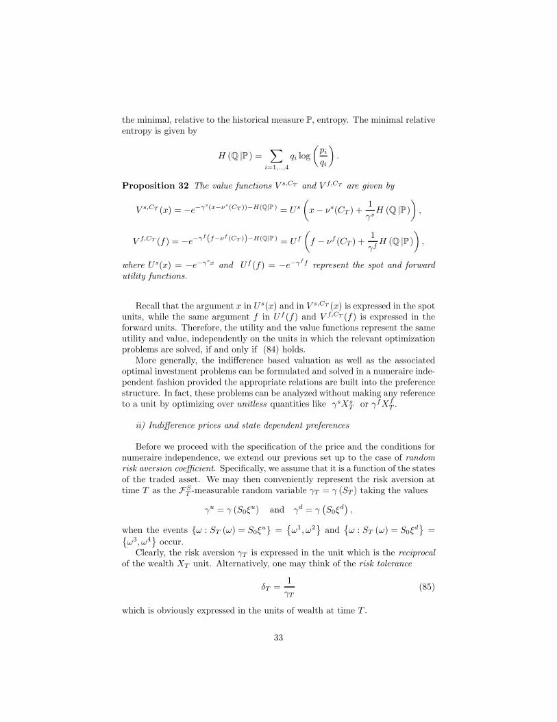
Recall that the argument x in Us(x) and in V s,CT (x) is expressed in the spotunits, while the same argument f in Uf (f) and V f,CT (f) is expressed in theforward units. Therefore, the utility and the value functions represent the sameutility and value, independently on the units in which the relevant optimizationproblems are solved, if and only if (84) holds.

More generally, the indifference based valuation as well as the associatedoptimal investment problems can be formulated and solved in a numeraire inde-pendent fashion provided the appropriate relations are built into the preferencestructure. In fact, these problems can be analyzed without making any referenceto a unit by optimizing over unitless quantities like γsXs

T or γfXfT .

ii) Indifference prices and state dependent preferences

Before we proceed with the specification of the price and the conditions fornumeraire independence, we extend our previous set up to the case of randomrisk aversion coefficient. Specifically, we assume that it is a function of the statesof the traded asset. We may then conveniently represent the risk aversion attime T as the FS

T -measurable random variable γT = γ (ST ) taking the values

γu = γ (S0ξu) and γd = γ

(S0ξ

d),

when the events ω : ST (ω) = S0ξu =

ω1, ω2

and

ω : ST (ω) = S0ξ

d

=ω3, ω4

occur.

Clearly, the risk aversion γT is expressed in the unit which is the reciprocalof the wealth XT unit. Alternatively, one may think of the risk tolerance

δT =1

γT(85)

which is obviously expressed in the units of wealth at time T .

33

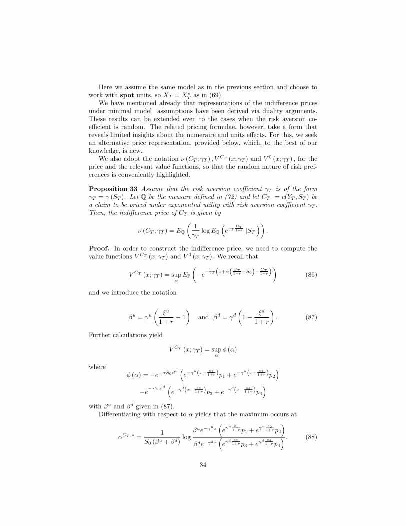
Here we assume the same model as in the previous section and choose towork with spot units, so XT = Xs

T as in (69).We have mentioned already that representations of the indifference prices

under minimal model assumptions have been derived via duality arguments.These results can be extended even to the cases when the risk aversion co-efficient is random. The related pricing formulae, however, take a form thatreveals limited insights about the numeraire and units effects. For this, we seekan alternative price representation, provided below, which, to the best of ourknowledge, is new.

We also adopt the notation ν (CT ; γT ) , V CT (x; γT ) and V 0 (x; γT ) , for theprice and the relevant value functions, so that the random nature of risk pref-erences is conveniently highlighted.

Proposition 33 Assume that the risk aversion coefficient γT is of the formγT = γ (ST ). Let Q be the measure defined in (72) and let CT = c(YT , ST ) bea claim to be priced under exponential utility with risk aversion coefficient γT .Then, the indifference price of CT is given by

ν (CT ; γT ) = EQ

(1

γTlog EQ

(eγT

CT1+r |ST

)).

Proof. In order to construct the indifference price, we need to compute thevalue functions V CT (x; γT ) and V 0 (x; γT ). We recall that

V CT (x; γT ) = supα

EP

(−e

−γT

“

x+α“

ST1+r

−S0

”

−CT1+r

”)

(86)

and we introduce the notation

βu = γu

(ξu

1 + r− 1

)and βd = γd

(1 −

ξd

1 + r

). (87)

Further calculations yield

V CT (x; γT ) = supα

φ (α)

whereφ (α) = −e−αS0βu

(e−γu(x−

c11+r )p1 + e−γu(x−

c21+r )p2

)

−e−αS0βd (

e−γd(x−c3

1+r )p3 + e−γd(x−c4

1+r )p4

)

with βu and βd given in (87).Differentiating with respect to α yields that the maximum occurs at

αCT ,∗ =1

S0 (βu + βd)log

βue−γux(eγu c1

1+r p1 + eγu c21+r p2

)

βde−γdx(eγd c3

1+r p3 + eγd c41+r p4

) . (88)

34

Calculating the terms −e−αCT ,∗S0βu

and −e−αCT ,∗S0βd

gives

e−αCT ,∗S0βu

=

(βu

βd

)− βu

βu+βd

eβu(γu

−γd)βu+βd x

(eγu c1

1+r p1 + eγu c21+r p2

eγd c31+r p3 + eγd c4

1+r p4

)− βu

βu+βd

and

e−αCT ,∗S0βd

=

(βu

βd

)− βd

βu+βd

eβd(γu

−γd)βu+βd x

(eγu c1

1+r p1 + eγu c21+r p2

eγd c31+r p3 + eγd c4

1+r p4

)− βd

βu+βd

.

It then follows, after tedious but routine calculations that

V CT (x; γT ) = φ(αCT ,∗

)

= −

(

βu

βd

)− βu

βu+βd

+

(βu

βd

) βd

βu+βd

e

− βuγd+βdγu

βu+βd x

×(eγu c1

1+r p1 + eγu c21+r p2

) βd

βu+βd(eγd c3

1+r p3 + eγd c41+r p4

) βu

βu+βd

. (89)

Substituting CT = 0 in turn implies

V 0 (x; γT ) = −

(

βu

βd

)− βu

βu+βd

+

(βu

βd

) βd

βu+βd

e−βuγd+βdγu

βu+βd x

× (p1 + p2)βd

βu+βd (p3 + p4)βu

βu+βd . (90)

Using (89), (90) and (4) (cf. Definition 1) we get

ν(CT ; γT ) =

(βuγd + βdγu

βu + βd

)−1

×

(βd

βu + βdlog

eγu c11+r p1 + eγu c2

1+r p2

p1 + p2+

βu

βu + βdlog

eγd c31+r p3 + eγd c4

1+r p4

p3 + p4

).

(91)We next observe that

γuβd

βuγd + βdγu=

(1 + r) − ξd

ξu − ξd(92)

=S0 (1 + r) − Sd

Su − Sd= q,

andγdβu

βuγd + βdγu=

ξu − (1 + r)

ξu − ξd

35

=Su − S0 (1 + r)

Su − Sd= 1 − q,

where Su = S0ξu and Sd = S0ξ

d. The above equalities combined with (91) thenyield

ν (CT ; γT ) = q1

γulog

eγu c11+r p1 + eγu c2

1+r p2

p1 + p2(93)

+ (1 − q)1

γdlog

eγd c31+r p3 + eγd c4

1+r p4

p3 + p4.

Following the arguments developed in the proof of Proposition 2 we see that

eγu c11+r p1 + eγu c2

1+r p2

p1 + p2= EQ

(eγT

CT1+r |ST = Su

)(94)

andeγd c3

1+r p3 + eγd c41+r p4

p3 + p4= EQ

(eγT

CT1+r

∣∣ST = Sd)

. (95)

Finally, using the equalities (94) and (95), and the expression in (93) we easilyconclude.

Proposition 34 Assume that the risk aversion coefficient γT is of the formγT = γ (ST ) and let δT be the risk tolerance coefficient introduced in (85). LetQ be the measure defined in (72) and let CT = c(YT , ST ) be a claim to be pricedunder exponential utility with risk aversion coefficient γT .

Then, the value functions V 0 (x; γT ) and V CT (x; γT ) , defined in (86), admitthe following representations

V 0 (x; γT ) = − exp

(−

x

EQ (δT )− H (Q∗ |P )

)(96)

V CT (x; γT ) = − exp

(−

x − ν (CT ; γT )

EQ (δT )− H (Q∗ |P )

)(97)

where

ν (CT ; γT ) = EQ

(1

γTlog EQ

(eγT

CT1+r |ST

))(98)

anddQ∗

dQ(ω) =

δT (ω)

EQ (δT ). (99)

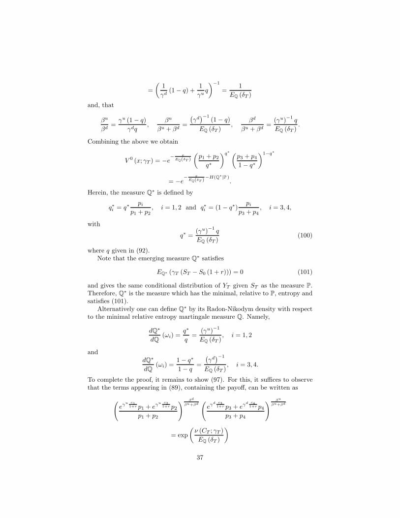
Proof. To show (96) and (97), we work with formulae (89) and (90) interpretingappropriately the involved quantities.

We first observe that

βuγd + βdγu

βu + βd=

(βu + βd

βuγd + βdγu

)−1

36

=

(1

γd(1 − q) +

1

γuq

)−1

=1

EQ (δT )

and, that

βu

βd=

γu (1 − q)

γdq,

βu

βu + βd=

(γd)−1

(1 − q)

EQ (δT ),

βd

βu + βd=

(γu)−1

q

EQ (δT ).

Combining the above we obtain

V 0 (x; γT ) = −e− x

EQ(δT )

(p1 + p2

q∗

)q∗ (p3 + p4

1 − q∗

)1−q∗

= −e− x

EQ(δT )−H(Q∗|P )

.

Herein, the measure Q∗ is defined by

q∗i = q∗pi

p1 + p2, i = 1, 2 and q∗i = (1 − q∗)

pi

p3 + p4, i = 3, 4,

with

q∗ =(γu)

−1q

EQ (δT )(100)

where q given in (92).Note that the emerging measure Q∗ satisfies

EQ∗ (γT (ST − S0 (1 + r))) = 0 (101)

and gives the same conditional distribution of YT given ST as the measure P.Therefore, Q∗ is the measure which has the minimal, relative to P, entropy andsatisfies (101).

Alternatively one can define Q∗ by its Radon-Nikodym density with respectto the minimal relative entropy martingale measure Q. Namely,

dQ∗

dQ(ωi) =

q∗

q=

(γu)−1

EQ (δT ), i = 1, 2

anddQ∗

dQ(ωi) =

1 − q∗

1 − q=

(γd)−1

EQ (δT ), i = 3, 4.

To complete the proof, it remains to show (97). For this, it suffices to observethat the terms appearing in (89), containing the payoff, can be written as

(eγu c1

1+r p1 + eγu c21+r p2

p1 + p2

) βd

βu+βd(

eγd c31+r p3 + eγd c4

1+r p4

p3 + p4

) βu

βu+βd

= exp

(ν (CT ; γT )

EQ (δT )

)

37

where we used (98). Formula (97) then follows from the latter equality, andassertions (89) and (96).

We stress that both measures, Q and Q∗, have minimal, relative to P, en-tropy. However, they have different martingales properties, namely, under Q,

EQ (ST − S0 (1 + r)) = 0,

while, under Q∗,EQ∗ (γT (ST − S0 (1 + r))) = 0.

We finish this section with an important decomposition result for the writer’soptimal policy.

Proposition 35 The writer’s optimal investment policy αCT ,∗ (cf. (88)) ad-mits the following decomposition

αCT ,∗ = α0,∗ + α1,∗ + α2,∗, (102)

where

α0,∗ = −∂H (Q∗ |P )

∂S0EQ (δT ) , α1,∗ =

∂ log EQ (δT )

∂S0x

and

α2,∗ = EQ (δT )∂

∂S0

(ν (CT ; γT )

EQ (δT )

).

Proof. We first recall that

αCT ,∗ =1

S0 (βu + βd)log

βue−γux(eγu c1

1+r p1 + eγu c21+r p2

)

βde−γdx(eγd c3

1+r p3 + eγd c41+r p4

) .

We then write αCT ,∗ as

αCT ,∗ = α0,∗ + α1,∗ + α2,∗

where

α0,∗ =1

S0 (βu + βd)log

βu (p1 + p2)

βd (p3 + p4),

α1,∗ =1

S0 (βu + βd)log

e−γux

e−γdx,

and

α2,∗ =1

S0 (βu + βd)log

(eγu c1

1+r p1 + eγu c21+r p2

)(p3 + p4)

(eγd c3

1+r p3 + eγd c41+r p4

)(p1 + p2)

.

38

We will next represent the various quantities in terms of the measures Q andQ∗. Recall that

q =S0 (1 + r) − Sd

Su − Sd,

∂q

∂S0=

1 + r

Su − Sd,

andβd

βu + βd=

(γu)−1 q

EQ (δT )= q∗,

βu

βu + βd=

(γd)−1

(1 − q)

EQ (δT )= 1 − q∗.

It follows, trivially, that

logβu (p1 + p2)

βd (p3 + p4)= log

(1 − q∗) (p1 + p2)

q∗ (p3 + p4).

Moreover, the relative entropy H (Q∗ |P ) is given by

H (Q∗ |P) = q∗ logq∗

p1 + p2+ (1 − q∗) log

1 − q∗

p3 + p4

and, hence,∂H (Q∗ |P)

∂S0= −

(∂q∗

∂S0

)log

(1 − q∗) (p1 + p2)

q∗ (p3 + p4).

The sensitivity of q∗ to S0 can be easily calculated. Indeed, we get

∂q∗

∂S0=

∂q

∂S0

(γu)−1 (

γd)−1

(EQ(δT ))2 .

Also, because the coefficient S0

(βu + βd

)can be written as

1

S0 (βu + βd)=

∂q

∂S0

(γu)−1 (

γd)−1

EQ(δT ),

we get1

S0 (βu + βd)=

∂q∗

∂S0EQ(δT ).

The above formulae imply that

α0,∗ = −∂H (Q∗ |P)

∂S0EQ(δT ).

Moving to the second term, α∗,1, we notice that

α∗,1 = −1

S0 (βu + βd)

(γu − γd

)x.

39

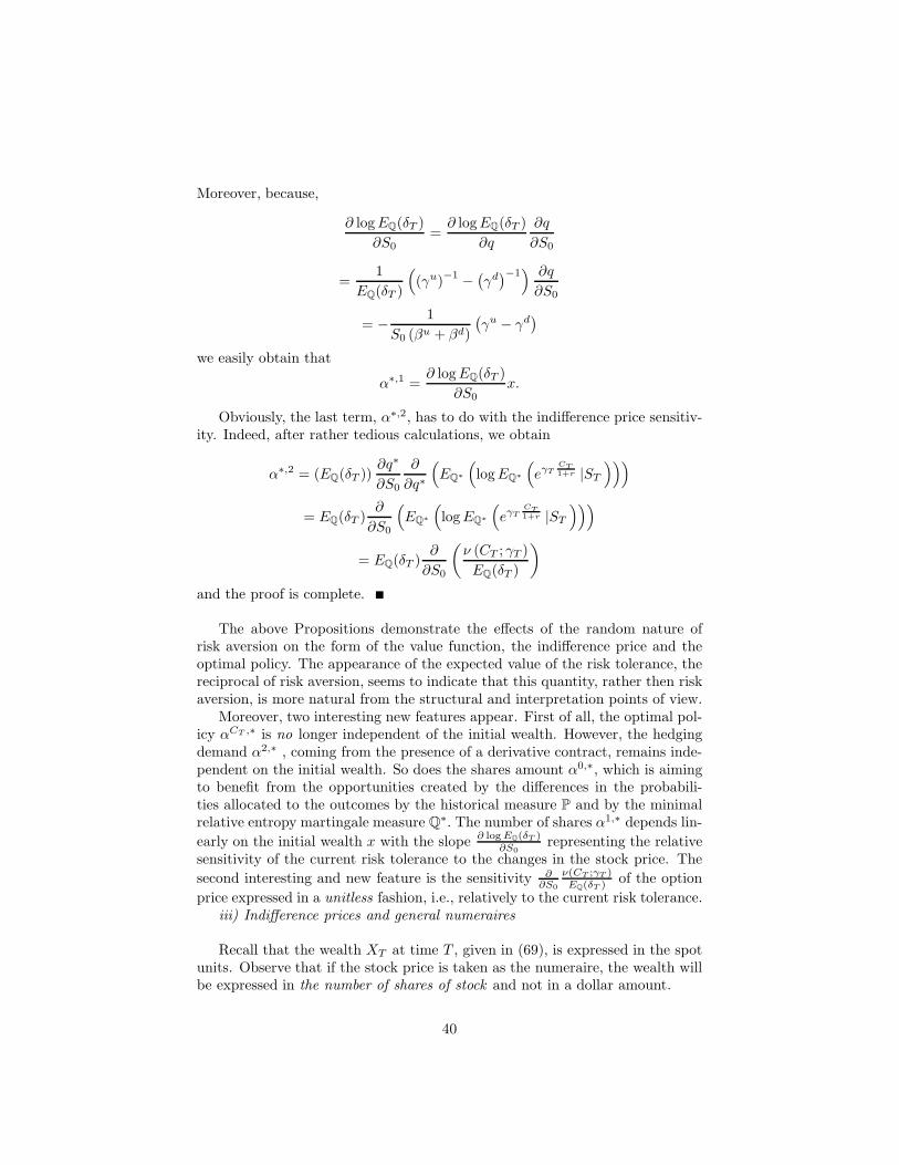
Moreover, because,

∂ log EQ(δT )

∂S0=

∂ log EQ(δT )

∂q

∂q

∂S0

=1

EQ(δT )

((γu)

−1−(γd)−1) ∂q

∂S0

= −1

S0 (βu + βd)

(γu − γd

)

we easily obtain that

α∗,1 =∂ log EQ(δT )

∂S0x.

Obviously, the last term, α∗,2, has to do with the indifference price sensitiv-ity. Indeed, after rather tedious calculations, we obtain

α∗,2 = (EQ(δT ))∂q∗

∂S0

∂

∂q∗

(EQ∗

(log EQ∗

(eγT

CT1+r |ST

)))

= EQ(δT )∂

∂S0

(EQ∗

(log EQ∗

(eγT

CT1+r |ST

)))

= EQ(δT )∂

∂S0

(ν (CT ; γT )

EQ(δT )

)

and the proof is complete.

The above Propositions demonstrate the effects of the random nature ofrisk aversion on the form of the value function, the indifference price and theoptimal policy. The appearance of the expected value of the risk tolerance, thereciprocal of risk aversion, seems to indicate that this quantity, rather then riskaversion, is more natural from the structural and interpretation points of view.

Moreover, two interesting new features appear. First of all, the optimal pol-icy αCT ,∗ is no longer independent of the initial wealth. However, the hedgingdemand α2,∗ , coming from the presence of a derivative contract, remains inde-pendent on the initial wealth. So does the shares amount α0,∗, which is aimingto benefit from the opportunities created by the differences in the probabili-ties allocated to the outcomes by the historical measure P and by the minimalrelative entropy martingale measure Q∗. The number of shares α1,∗ depends lin-

early on the initial wealth x with the slope ∂ log EQ(δT )∂S0

representing the relativesensitivity of the current risk tolerance to the changes in the stock price. The

second interesting and new feature is the sensitivity ∂∂S0

ν(CT ;γT )EQ(δT ) of the option

price expressed in a unitless fashion, i.e., relatively to the current risk tolerance.iii) Indifference prices and general numeraires

Recall that the wealth XT at time T , given in (69), is expressed in the spotunits. Observe that if the stock price is taken as the numeraire, the wealth willbe expressed in the number of shares of stock and not in a dollar amount.

40

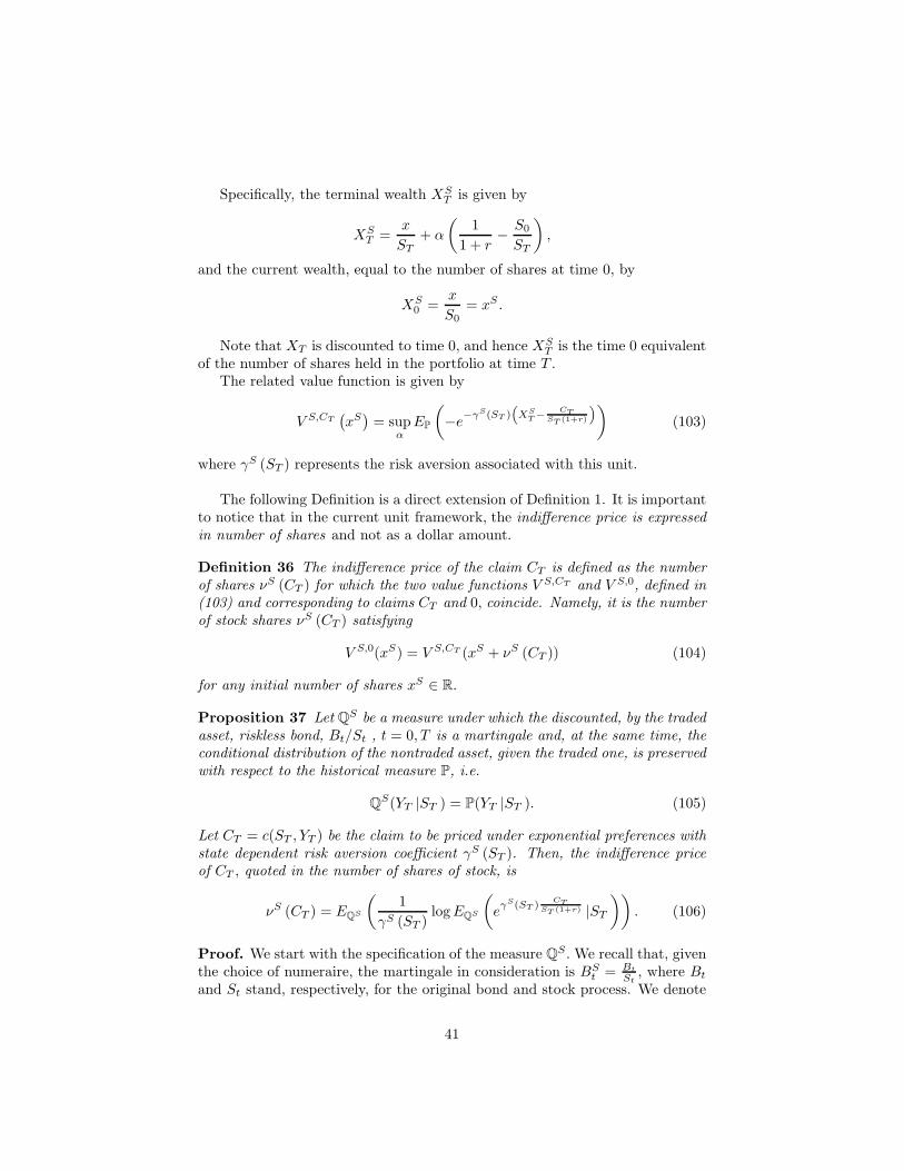
Specifically, the terminal wealth XST is given by

XST =

x

ST+ α

(1

1 + r−

S0

ST

),

and the current wealth, equal to the number of shares at time 0, by

XS0 =

x

S0= xS .

Note that XT is discounted to time 0, and hence XST is the time 0 equivalent

of the number of shares held in the portfolio at time T .The related value function is given by

V S,CT(xS)

= supα

EP

(−e

−γS(ST )“

XST −

CTST (1+r)

”)

(103)

where γS (ST ) represents the risk aversion associated with this unit.

The following Definition is a direct extension of Definition 1. It is importantto notice that in the current unit framework, the indifference price is expressedin number of shares and not as a dollar amount.

Definition 36 The indifference price of the claim CT is defined as the numberof shares νS (CT ) for which the two value functions V S,CT and V S,0, defined in(103) and corresponding to claims CT and 0, coincide. Namely, it is the numberof stock shares νS (CT ) satisfying

V S,0(xS) = V S,CT (xS + νS (CT )) (104)

for any initial number of shares xS ∈ R.

Proposition 37 Let QS be a measure under which the discounted, by the tradedasset, riskless bond, Bt/St , t = 0, T is a martingale and, at the same time, theconditional distribution of the nontraded asset, given the traded one, is preservedwith respect to the historical measure P, i.e.

QS(YT |ST ) = P(YT |ST ). (105)

Let CT = c(ST , YT ) be the claim to be priced under exponential preferences withstate dependent risk aversion coefficient γS (ST ). Then, the indifference priceof CT , quoted in the number of shares of stock, is

νS (CT ) = EQS

(1

γS (ST )log EQS

(e

γS(ST )CT

ST (1+r) |ST

)). (106)

Proof. We start with the specification of the measure QS. We recall that, giventhe choice of numeraire, the martingale in consideration is BS

t = Bt

St, where Bt

and St stand, respectively, for the original bond and stock process. We denote

41

by qSi , i = 1, .., 4 the elementary probabilities of QS . Simple calculations yield

that

qSi = qS pi

p1 + p2, i = 1, 2 and qS

i = (1 − qS)pi

p3 + p4, i = 3, 4,

where

qS =

(1

ξd−

1

1 + r

)ξuξd

ξu − ξd.

Alternatively, the measure QS can be defined by its Radon-Nikodym densitywith respect to the measure Q, namely

dQS

dQ=

ST

(1 + r) S0.

Indeed, we have

EQS

(1 + r

ST

)= EQ

(ST

(1 + r) S0

1 + r

ST

)=

1

S0.

We next observe that the value function V S,CT (cf. (103)) can be written as

V S,CT(xS)

= supα

EP

(−e

−λT

“

x+α“

ST1+r

−S0

”

−CT1+r

”)

,

where

λT =γS (ST )

ST. (107)

Working as in the proof of Proposition 35 we get

V S,CT(xS)

= V CT (x; λT )

= − exp

(−

x − ν (CT ; λT )

EQ

(λ−1

T

) − H(Q |P

))

wheredQ

dQ=

λ−1T

EQ

(λ−1

T

) .

The wealth argument x in V CT (x; λT ) as well as the price

ν (CT ; λT ) = EQ

(1

λTlog EQ

(eλT

CT1+r |ST

))

are expressed in the spot units and, hence, for all claims CT we have

ν (CT ; γT ) = ν (CT ; λT ) .

42

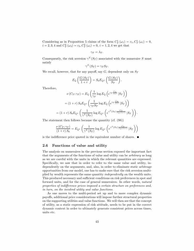
Considering as in Proposition 5 claims of the form C1T (ω1) = c1, C

1T (ωi) = 0,

i = 2, 3, 4 and C2T (ω3) = c3, C

2T (ωi) = 0, i = 1, 2, 4 we get that

γT = λT .

Consequently, the risk aversion γS (ST ) associated with the numeraire S mustsatisfy

γS (ST ) = γT ST .

We recall, however, that for any payoff, say G, dependent only on ST

EQ

(G (ST )

1 + r

)= S0EQS

(G (ST )

ST

).

Therefore,

ν (CT ; γT ) = EQ

(1

γTlog EQ

(eγT

CT1+r |ST

))

= (1 + r) S0EQS

(1

γT STlog EQ

(eγT

CT1+r |ST

))

= (1 + r) S0EQS

(1

γS (ST )log EQS

(e

γS(ST )CT

ST (1+r) |ST

)).

The statement then follows because the quantity (cf. (98))

ν (CT ; γT )

(1 + r) S0= EQS

(1

γS (ST )log EQS

(e

γS(ST )CT

ST (1+r) |ST

))

is the indifference price quoted in the equivalent number of shares.

2.6 Functions of value and utility

The analysis on numeraires in the previous section exposed the important factthat the arguments of the functions of value and utility can be arbitrary as longas we are careful with the units in which the relevant quantities are expressed.Specifically, we saw that in order to refer to the same value and utility, in-dependently on the arguments, and, also, in order to eliminate static arbitrageopportunities from our model, one has to make sure that the risk aversion multi-plied by wealth represents the same quantity independently on the wealth units.This produced necessary and sufficient conditions on risk preferences in spot andforward units, and for the case of general numeraires. In other words, naturalproperties of indifference prices imposed a certain structure on preferences and,in turn, on the involved utility and value functions.

As one moves to the multi-period set up and to more complex dynamicpayoffs, additional price considerations will impose further structural propertieson the supporting utilities and value functions. We will then see that the conceptof utility, as a static expression of risk attitude, needs to be put in the correctdynamic context in order to ultimately generate consistent prices across times,units etc.

43

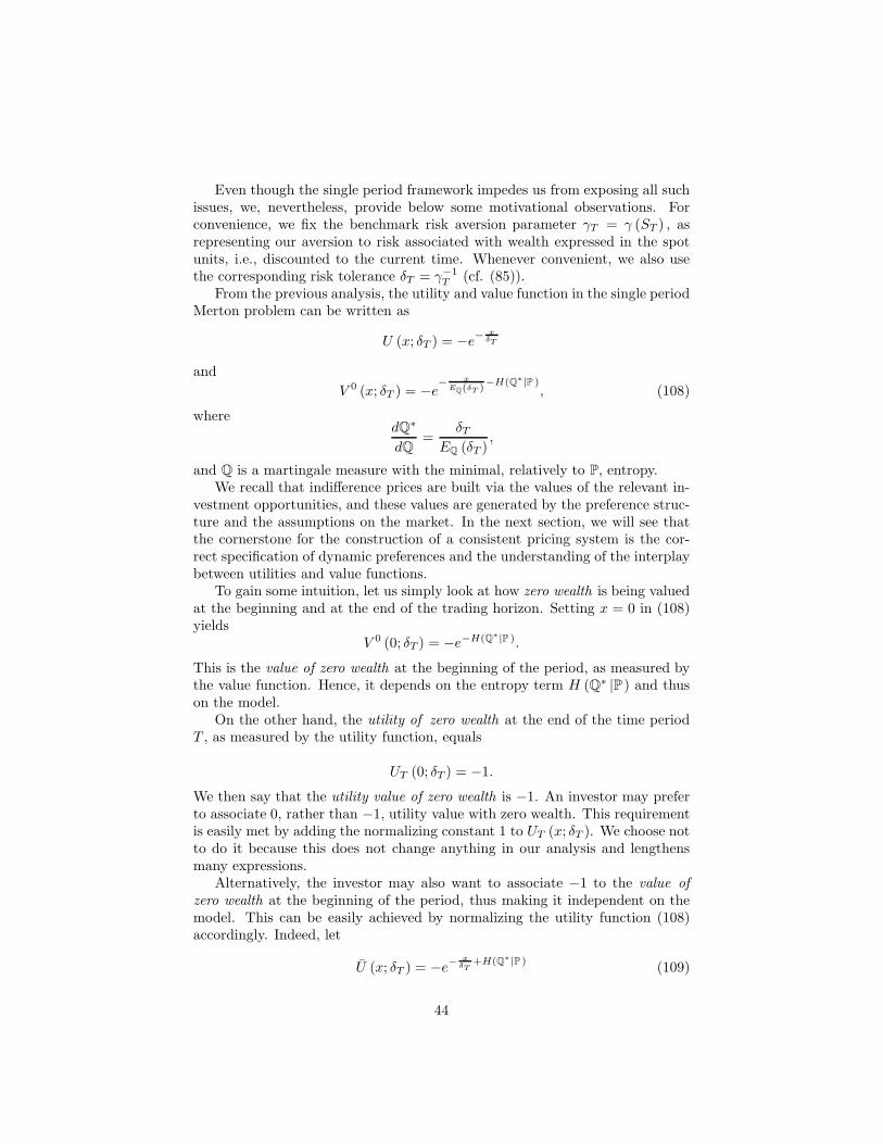
Even though the single period framework impedes us from exposing all suchissues, we, nevertheless, provide below some motivational observations. Forconvenience, we fix the benchmark risk aversion parameter γT = γ (ST ) , asrepresenting our aversion to risk associated with wealth expressed in the spotunits, i.e., discounted to the current time. Whenever convenient, we also usethe corresponding risk tolerance δT = γ−1

T (cf. (85)).From the previous analysis, the utility and value function in the single period

Merton problem can be written as

U (x; δT ) = −e− x

δT

and

V 0 (x; δT ) = −e− x

EQ(δT )−H(Q∗|P )

, (108)

wheredQ∗

dQ=

δT

EQ (δT ),

and Q is a martingale measure with the minimal, relatively to P, entropy.We recall that indifference prices are built via the values of the relevant in-

vestment opportunities, and these values are generated by the preference struc-ture and the assumptions on the market. In the next section, we will see thatthe cornerstone for the construction of a consistent pricing system is the cor-rect specification of dynamic preferences and the understanding of the interplaybetween utilities and value functions.

To gain some intuition, let us simply look at how zero wealth is being valuedat the beginning and at the end of the trading horizon. Setting x = 0 in (108)yields

V 0 (0; δT ) = −e−H(Q∗|P ).

This is the value of zero wealth at the beginning of the period, as measured bythe value function. Hence, it depends on the entropy term H (Q∗ |P ) and thuson the model.

On the other hand, the utility of zero wealth at the end of the time periodT , as measured by the utility function, equals

UT (0; δT ) = −1.

We then say that the utility value of zero wealth is −1. An investor may preferto associate 0, rather than −1, utility value with zero wealth. This requirementis easily met by adding the normalizing constant 1 to UT (x; δT ). We choose notto do it because this does not change anything in our analysis and lengthensmany expressions.

Alternatively, the investor may also want to associate −1 to the value ofzero wealth at the beginning of the period, thus making it independent on themodel. This can be easily achieved by normalizing the utility function (108)accordingly. Indeed, let

U (x; δT ) = −e− x

δT+H(Q∗|P )

(109)

44

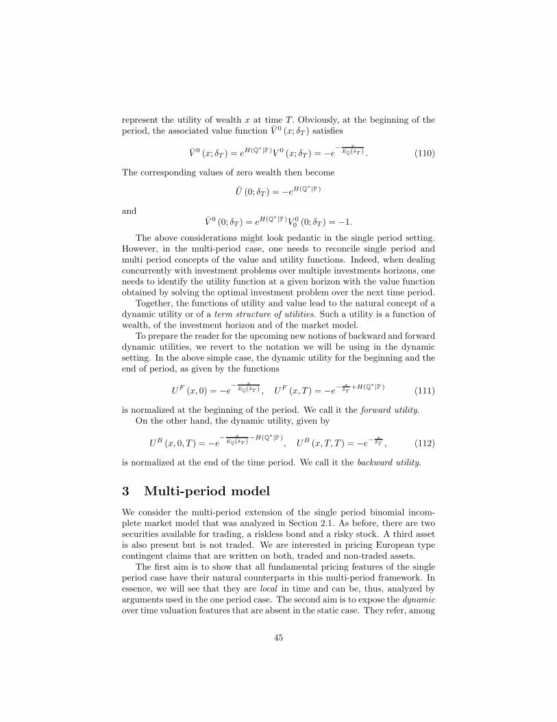
represent the utility of wealth x at time T. Obviously, at the beginning of theperiod, the associated value function V 0 (x; δT ) satisfies

V 0 (x; δT ) = eH(Q∗|P )V 0 (x; δT ) = −e− x

EQ(δT ) . (110)

The corresponding values of zero wealth then become

U (0; δT ) = −eH(Q∗|P )

andV 0 (0; δT ) = eH(Q∗|P )V 0

0 (0; δT ) = −1.

The above considerations might look pedantic in the single period setting.However, in the multi-period case, one needs to reconcile single period andmulti period concepts of the value and utility functions. Indeed, when dealingconcurrently with investment problems over multiple investments horizons, oneneeds to identify the utility function at a given horizon with the value functionobtained by solving the optimal investment problem over the next time period.

Together, the functions of utility and value lead to the natural concept of adynamic utility or of a term structure of utilities. Such a utility is a function ofwealth, of the investment horizon and of the market model.

To prepare the reader for the upcoming new notions of backward and forwarddynamic utilities, we revert to the notation we will be using in the dynamicsetting. In the above simple case, the dynamic utility for the beginning and theend of period, as given by the functions

UF (x, 0) = −e− x

EQ(δT ) , UF (x, T ) = −e− x

δT+H(Q∗|P )

(111)

is normalized at the beginning of the period. We call it the forward utility.On the other hand, the dynamic utility, given by

UB (x, 0, T ) = −e− x

EQ(δT )−H(Q∗|P )

, UB (x, T, T ) = −e− x

δT , (112)

is normalized at the end of the time period. We call it the backward utility.

3 Multi-period model

We consider the multi-period extension of the single period binomial incom-plete market model that was analyzed in Section 2.1. As before, there are twosecurities available for trading, a riskless bond and a risky stock. A third assetis also present but is not traded. We are interested in pricing European typecontingent claims that are written on both, traded and non-traded assets.

The first aim is to show that all fundamental pricing features of the singleperiod case have their natural counterparts in this multi-period framework. Inessence, we will see that they are local in time and can be, thus, analyzed byarguments used in the one period case. The second aim is to expose the dynamicover time valuation features that are absent in the static case. They refer, among

45

others, to the dynamic nature of risk preferences and the semigroup propertyof the proposed pricing schemes.

The claim in consideration is taken to yield payoff CT at expiration T . Weaim at representing its indifference price, at time t < T , in a natural valuationformat, namely,

νt(CT ) = E(t,T )(CT ) (113)

where E(t,T ) stands for the appropriate dynamic pricing operator.A fundamental property that the operator E(t,T ) should have is the semigroup

property,

νt(CT ) = E(t,s)(E(s,T )(CT )) = E(t,s)(νs(CT )) for t ≤ s ≤ T. (114)

This states that the price νt(CT ) can be computed in two steps in reference to anintermediate time t ≤ s ≤ T . Namely, one may first determine the indifferenceprice at time s, νs(CT ) = E(s,T )(CT ), by applying (113), and, then, use νs(CT )as a new claim to be priced at initial time t. Clearly, this property states thatthe current price can serve as a new payoff which is, in turn, priced, movingbackwards in time, via the time-adjusted price operator. If property (114) fails,it is easy to see that arbitrage opportunities may arise.

We recall that, in the single period case (r = 0), the indifference price wasrepresented in terms of the nonlinear valuation functional

ν(CT ) = EQ(CT ) = EQ(1

γlog EQ(eγCT |ST )) (115)

(cf. (9)). The indifference pricing measure Q turned out to be the uniquemartingale measure that satisfies

Q(YT |ST ) = P(YT |ST ). (116)

Given the inherent non-linearities of the indifference pricing mechanism, westress that, a priori, it is not at all obvious what are the multi-period analoguesof (115) and (116), and why the semigroup price property (114) must follow. Wewill see that there is a delicate interplay among optimality of policies, semigroupproperties of the involved value functions, the nature of the pricing measure andthe structure of the pricing schemes that ultimately yields the desired pricingingredients.

An important issue that emerges once the market environment becomesdynamic is the proper specification of preferences across times and investmentopportunities. This leads us to the development of dynamic utilities. Two kindsof such utilities are considered, namely, the backward and the forward ones.With reference to these dynamic risk preferences, we introduce the backwardand forward indifference prices and construct their associated pricing schemes.While the backward utility and forward price are, in many aspects, similar tothe traditional value function and classical indifference price, the concepts offorward utility and forward indifference price are, to the best of our knowledge,entirely new.

46

3.1 Preliminaries

We start with the probabilistic set-up of the multi-period model. We denote bySt, t = 0, 1, ... the values of the traded risky asset. It is assumed that St > 0,and we define the variables ξt as

ξt+1 =St+1

St, ξt+1 = ξd

t+1, ξut+1 with 0 < ξd

t+1 < 1 < ξut+1.

The second traded asset is riskless and yields zero interest rate. We also denoteby Yt, t = 0, 1, .., the values of the non-traded asset and we assume that, for allt = 0, 1, ..T, Yt 6= 0. We introduce the variables ηt satisfying

ηt+1 =Yt+1

Yt, ηt+1 = ηd

t+1, ηut+1 with ηd

t+1 < ηut+1.

We then view St, Yt : t = 0, 1, ... as a two-dimensional stochastic processdefined on the probability space (Ω,F , (Ft) , P). The filtration Ft is generated bythe random variables Ss and Ys, or, equivalently, by ξs and ηs, for s = 0, 1, ..., t.We also consider the filtrations FS

t an FYt generated, respectively, by Ss and

Ys for s = 0, 1, ..., t. The real (historical) probability measure on Ω and F isdenoted by P.

Using notation compatible with the single period case, we take Xt, t = 0, 1, ...to represent the wealth process associated with a multi-period self-financingportfolio. We denote by αt, t = 0, 1, ... the number of shares of the traded assetheld in this portfolio over the time period [t − 1, t). Then,

Xt = Xt − Xt−1 = αt St

and, hence, for t = 0, 1, .., T − 1,

XT = Xt +

T∑

s=t+1

αs Ss.

Consider the optimal investment problem over the trading horizon [t, T ] andassume, for the moment, that the investor has exponential risk preferences ofconstant absolute risk aversion γ > 0. This assumption will be removed whenthe dynamic, backward and forward, risk preferences are introduced.

The investor aims at maximizing the expected utility of terminal wealth XT .For t = 0, 1, .., T − 1, the associated value function, corresponding to wealth xat time t, is then defined by

V (x, t) = supαt+1,...,αT

EP

(−e−γXT |Ft

)(117)

= supαt+1,...,αT

EP

(−e−γ(x+

PTs=t+1 αsSs) |Ft

).

47

This is the classical value function, studied, among others, by Rouge and ElKaroui (2000), Delbaen et al. (2002) (see, also, Kabanov and Stricker (2002))who established that, for t = 0, 1, .., T − 1,

V (x, t) = −e−γx−HT (Q(·|Ft )| P(·|Ft ) ).

Herein, Q is a martingale measure, defined on FT , that has the minimal,relative to P (restricted to FT ) entropy. The quantity HT (Q (· |Ft ) | P (· |Ft ) )denotes the aggregate relative entropy of the conditional on Ft measures P (· |Ft )and Q (· |Ft ), defined on FT , namely,

HT (Q (· |Ft ) | P (· |Ft ) ) = EQ

(log

Q (· |Ft )

P (· |Ft )|Ft

).

The relative entropy will play an important role in the pricing and specificationof dynamic risk preferences. The following result provides an analytic expressionfor it.

Proposition 38 Let Q be an equivalent to P martingale measure, defined onFT and having the minimal, relative to P, entropy. For all t = 0, 1, .., T − 1,let Q (· |Ft ) and P (· |Ft ) be defined on FT and standing for the conditional, onFt, measures. Then, their relative entropy, HT (Q (· |Ft ) | P (· |Ft ) ), is given by

HT (Q (· |Ft ) | P (· |Ft ) ) = EQ

(T∑

s=t+1

hs |Ft

), (118)

where, for s = t + 1, ..., T,

hs = Hs (Q (· |Fs−1 ) |P (· |Fs−1 ) )

= qs logqs

P (As |Fs−1 )+ (1 − qs) log

1 − qs

1 − P (As |Fs−1 )≥ 0, (119)

As = ξs = ξus

and

qs = Q (As |Fs−1 ) =1 − ξd

s

ξus − ξd

s

.

Proof. Let Q be an equivalent to P martingale measure on FT . Recall that,for any Q, the conditional on Ft measure Q (· |Ft ) is defined by

Q (A |Ft ) = EQ (IA |Ft ) , A ∈ FT .

Recall also that the, relative to P( · |Ft ), entropy of Q(· |Ft ) is given by

HT (Q (· |Ft ) |P (· |Ft ) )

48

= EQ

(log

∏T−1s=t Q (ξs+1, ηs+1 |Fs )

∏T−1s=t P (ξs+1, ηs+1 |Fs )

|Ft

)

=

T−1∑

s=t

EQ

(log

Q (ξs+1, ηs+1 |Fs )

P (ξs+1, ηs+1 |Fs )|Ft

),

where we used that

P(ξt+1, ..., ξT , ηt+1, ..., ηT |Ft ) =

T−1∏

s=t

P (ξs+1, ηs+1 |Fs )

and

Q(ξt+1, ..., ξT , ηt+1, ..., ηT |Ft ) =

T−1∏

s=t

Q (ξs+1, ηs+1 |Fs ) .

To calculate the minimal relative entropy, it suffices to minimize the individualterms of the above sum. To this end, for s = t + 1, .., T , we look at theelementary events

As = ξs = ξus , Bs = ηs = ηu

s (120)

and we observe that,

EQ

(log

Q (ξs, ηs |Fs−1 )

P (ξs, ηs |Fs−1 )|Ft

)

= EQ

(log

Q (AsBs |Fs−1 )

P (AsBs |Fs−1 )IAsBs

+ logQ (AsB

cs |Fs−1 )

P (AsBcs |Fs−1 )

IAsBcs|Ft

)

+EQ

(log

Q (AcsBs |Fs−1 )

P (AcsBs |Fs−1 )

IAcsBs

+ logQ (Ac

sBcs |Fs−1 )

P (AcsB

cs |Fs−1 )

IAcsBc

s|Ft

).

In turn,

EQ

(log

Q (ξs, ηs |Fs−1 )

P (ξs, ηs |Fs−1 )|Ft

)= EQ

(Q (AsBs |Fs−1 ) log

Q (AsBs |Fs−1 )

P (AsBs |Fs−1 )

+ (Q (As |Fs−1 ) − Q (AsBs |Fs−1 )) logQ (As |Fs−1 ) − Q (AsBs |Fs−1 )

P (As |Fs−1 ) − P (AsBs |Fs−1 )|Ft

)

+EQ

((Q (Ac

s |Fs−1 ) − Q (AcsB

cs |Fs−1 )) log

Q (Acs |Fs−1 ) − Q (Ac

sBcs |Fs−1 )

P (Acs |Fs−1 ) − P (Ac

sBcs |Fs−1 )

+Q (AcsB

cs |Fs−1 ) log

Q (AcsB

cs |Fs−1 )

P (AcsB

cs |Fs−1 )

|Ft

),

where Acs and Bc

s stand for the complements of the events As and Bs. Recallthat, for any martingale measure,

Q (As |Fs−1 ) = qs =1 − ξd

s

ξus − ξd

s

.

49

Therefore, one needs to minimize the above two conditional expectations onlywith respect to the probabilities Q (AsBs |Fs−1 ) and Q (Ac

sBcs |Fs−1 ). Note

however, that this minimization problem is analogous to the one already solvedin the single period case. Straightforward, albeit tedious, arguments then yieldthat the martingale measure Q at which the minimum occurs, is unique andneeds to satisfy, for s = t + 1, ..., T,

Q (AsBs |Fs−1 )

Q (As |Fs−1 )=

P (AsBs |Fs−1 )

P (As |Fs−1 )(121)

andQ (Ac

sBcs |Fs−1 )

Q (Acs |Fs−1 )

=P (Ac

sBcs |Fs−1 )

P (Acs |Fs−1 )

. (122)

Consequently, for any martingale measure Q,

EQ

(log

Q (ξs, ηs |Fs−1 )

P (ξs, ηs |Fs−1 )|Ft

)≥ EQ

(log

Q (ξs, ηs |Fs−1 )

P (ξs, ηs |Fs−1 )|Ft

)

= EQ

(qs

P (AsBs |Fs−1 )

P (As |Fs−1 )log

qs

P (As |Fs−1 )

+qs

(1 −

P (AsBs |Fs−1 )

P (As |Fs−1 )

)log

qs

P (As |Fs−1 )|Ft

)

+EQ

((1 − qs)

(1 −

P (AcsB

cs |Fs−1 )

P (Acs |Fs−1 )

)log

1 − qs

1 − P (As |Fs−1 )

+ (1 − qs)P (Ac

sBcs |Fs−1 )

P (Acs |Fs−1 )

log1 − qs

1 − P (As |Fs−1 )|Ft

)

= EQ

(qs log

qs

P (As |Fs−1 )+ (1 − qs) log

1 − qs

1 − P (As |Fs−1 )|Ft

).

Finally, observe that the function

h (q) = q logq

p+ (1 − q) log

1 − q

1 − p, 0 < q < 1,

satisfies

h′ (q) = logq

p− log

1 − q

1 − pand h′′ (q) =

1

q+

1

1 − q.

Thereforeh (q) ≥ h (p) = 0

and the result follows.In the sequel, we extend the martingale measure Q to the σ-algebra F .

Consequently, both measures, P and Q are defined on F , and the relevantentropy terms of their restrictions to the σ-algebra FT are given by (118) and(119). Note that, with a slight abuse of notation, we use P and Q to denote themeasures of F as well as their restrictions to FT .

We observe that (121) and (122) can be written in the more compact form(123), appearing below. This, together with the above Proposition, leads us tothe following result.

50

Proposition 39 Let Q be a martingale measure that satisfies

Q(ηt+1

∣∣Ft ∨ FSt+1

)= P

(ηt+1

∣∣Ft ∨ FSt+1

), (123)

for t = 0, 1.., T − 1. Then Q is unique and it has the minimal, relative to P ,entropy.

3.2 Backward and forward dynamic utilities

The reader is referred back to the Introduction for a general motivation behindthe concept of dynamic risk preferences and to Section 2.6 for a preliminarydiscussion on backward and forward2 dynamic utilities. Before we move tothe multi-period setting, we illustrate the main ideas using a simple two-periodexample. We then give general definitions of the dynamic backward and forwardutilities and analyze their properties to the specific multi-period setting.

Let us consider an investor with an initial capital x who chooses to optimizehis wealth over the investment horizon T = 2, using the exponential utilityU (x; 2) = −e−γx, x ∈ R and γ > 0. The earlier results show that the associatedvalue function, given in (117) and now denoted by V (x, t; 2), satisfies, for t =0, 1,

V (x, 0; 2) = −e−γx−EQ(h1+h2|F0) and V (x, 1; 2) = −e−γx−EQ(h2|F1).

Herein hi, i = 1, 2, is given in (119), and F1 and F0 represent, respectively, theσ-algebras generated by both risks, at t = 1 and t = 0. We carry the notationwith regards to the trivial σ-algebra F0 for consistency.

Alternatively, the investor can also choose to optimize his wealth only overthe first time period, that is to choose as investment horizon T = 1. If he choosesagain the exponential utility at this new horizon, i.e. if U (x; 1) = −e−γx, theassociated value function becomes

V (x, 0; 1) = −e−γx−EQ(h1|F0).

Clearly, for all wealth levels x, we have that V (x, 0; 2) ≥ V (x, 0; 1) and thatV (x, 0; 2) > V (x, 0; 1) , if and only if P (A2 |F1 ) 6= q2. Consequently, the in-vestor gets more value (in terms of the value function) from the longer terminvestment, unless the historical and the risk neutral measures coincide. Thisstrongly suggests that he should never choose to optimize his wealth solely dur-ing the first period.

Note though that, in general, the investor would face the problem of choosinghis investment horizon. Moreover, once she has made her choice, she will staywith it regardless of any additional information about the market revealed inupcoming times. Alternatively, the investor may want to become indifferent to

2With a slight abuse, the ‘forward’ terminology is being used both for the correspondingdynamic utilities and the relevant wealth units. These two concepts are entirely different sincethe former corresponds to the evolution of the utility level across time while the latter in theunit choice.

51

the investment horizon. To achieve this goal, she may be prepared to modifyher utility functions for T = 1, or for T = 2, or, in general, for both investmenthorizons. In what follows, we will see that such an approach is in accordancewith the desire to formulate individual preferences in relation to the marketdynamics, rather than in complete isolation from them.

To gain some intuition, let us see if, indeed, for an appropriate choice ofpreferences, the investor’s value function becomes invariant with regards to theinvestment horizon. For this, let us fix the future terminal time T = 2 andconsider the backward dynamic utility, UB (x, t; 2), t = 0, 1, 2, defined by

UB (x, t; 2) =

−e−γx−EQ(h1+h2|F0) t = 0−e−γx−EQ(h2|F1) t = 1

−e−γx t = 2.

We adopt the terminology that UB (x, t; 2) is normalized at T = 2, in thatUB (x, 2; 2) = −e−γx.

We next introduce the associated backward dynamic value function V B (x, 0, t; 2)by

V B (x, 0, t; 2) = supα1,αt

EP

(UB (Xt, t; 2) |F0

)for t = 1, 2,

with X0 = x and Xt = x +∑t

s=1 αs Ss. We are going to calculate the valuesV B (x, 0, t; 2) for t = 0, 1, 2, corresponding to the different choices of tradinghorizon [0, t]. For t = 0, it is, naturally, taken that

V B (x, 0, 0; 2) = −e−γx−EQ(h1+h2|F0).

For the trading horizon [0, 1], we have

V B (x, 0, 1; 2) = supα1

EP

(UB (X1, 1; 2) |F0

)

= supα1

EP

(−e−γ(x+α1∆S1)−EQ(h2|F1) |F0

)

= supα1

EP

(e−γ(x+α1∆S1) sup

α2

EP

(−e−γα2∆S2 |F1

)|F0

).

Above we used that

−e−EQ(h2|F1) = supα2

EP

(−e−γα2∆S2 |F1

),

which follows from a direct adaptation of the arguments used in the single periodcase.

Therefore, the value of V B (x, 0, 1; 2) turns out to be

V B (x, 0, 1; 2) = supα1,α2

EP

(−e−γ(x+α1∆S1+α2∆S2) |F0

)

= −e−γx−EQ(h1+h2|F0).

52

For the trading horizon [0, 2] we, in turn, obtain

V B (x, 0, 2; 2) = supα1,α2

EP

(UB (X2, 2; 2) |F0

)

= supα1

EP

(e−γ(x+α1∆S1) sup

α2

E(−eγα2∆S2 |F1

)|F0

)

= −e−γx−EQ(h1+h2|F0 ).

The above calculations demonstrate that under the dynamic utility UB, theassociated dynamic value function (maximal expected dynamic utility) V B re-mains invariant with respect to the investment horizon, in that

V B (x, 0, 0; 2) = V B (x, 0, 1; 2) = V B (x, 0, 2; 2) (124)

= −e−γx−EQ(h1+h2|F0 ) for x ∈ R.

Note that the term V B (x, 0, 1; 2) represents, under the above risk prefer-ences, the value the investor gets from investing optimally over the first period(T = 1), while the term V B (x, 0, 2; 2) yields the value he gets from investingoptimally over two periods (T = 2).

The above concept of utility, normalized at some future time, resemblesin spirit the concept of a forward rate. Indeed, the dynamic backward utilityconverges at the normalization point to the classical exponential utility, in muchthe same way as the forward rate converges to the spot rate. Additionally, inanalogy to the notions of the savings account and of the associated spot rate,we also introduce the concept of dynamic utility which is normalized at initialtime, taken for simplicity to be 0, and which makes the investor indifferent tothe choice of any future investment horizon.

To provide some motivation for the upcoming notion of forward dynamicutility, we look at the following example. We fix the current time at 0, and wedefine the utility process UF (x, t; 0) , for t = 0, 1, 2, by

UF (x, t; 0) =

−e−γx t = 0−e−γx+h1 t = 1

−e−γx+Σ2i=1hi t = 2,

with hi, i = 1, 2 as in (119). We observe that UF (x, t; 0) is normalized at t = 0,since UF (x, 0; 0) = −e−γx for x ∈ R.

We next define the associated forward dynamic value function by

V F (x, 0, t; 0) = supα1,αt

EP

(UF (Xt, t; 0) |F0

)for t = 1, 2,

with X0 = x and Xt = x +∑t

i=1 αi Si. We are going to calculate the valuesV F (x, 0, t; 0) for t = 0, 1, 2, corresponding to the different choices of tradinghorizon [0, t]. For t = 0, we naturally have

V F (x, 0, 0; 0) = −e−γx

53

for x ∈ R, which yields that V F is itself normalized at t = 0.For the trading horizon [0, 1], we obtain

V F (x, 0, 1; 0) = supα1

EP

(UF (X1, 1; 0) |F0

)

= supα1

EP

(−e−γX1+h1 |F0

)

= supα1

EP

(−e−γ(x+α1S1)+h1 |F0

)

= e−γx supα1

EP

(−e−α1S1+h1 |F0

)= −e−γx.

Finally, for the trading horizon [0, 2], we have

V F (x, 0, 2; 0) = supα1,α2

EP

(UF (X2, 2; 0) |F0

)

= supα1,α2

EP

(EP

(−e−γX2+(h1+h2) |F1

)|F0

)

= supα1

EP

(supα2

EP

(−e−γX2+(h1+h2) |F1

)|F0

)

= supα1

EP

(e−γX1+h1 sup

α2

EP

(−e−γα2S2+h2 |F1

)|F0

)

= supα1

EP

(−e−γX1+h1 |F0

)

= supα1

EP

(UF (X1, 1; 0) |F0

)

= V F (x, 0, 1; 0) = −e−γx.

Therefore, the above choice of forward dynamic preferences yields, for t =0, 1, 2 and x ∈ R,

V F (x, 0, 0; 0) = V F (x, 0, 1; 0) (125)

= V F (x, 0, 2; 0) = −e−γx,

which, in turn, implies that the forward dynamic value function is invariantwith regards to the investment horizon.

We are now ready to introduce the above concepts in the general multi-periodsetting. We start with an auxiliary definition.

For convenience we recall the local entropy terms, (cf. (119)),

hi = qi logqi

P (Ai |Fi−1 )+ (1 − qi) log

1 − qi

1 − P (Ai |Fi−1 )

with

Ai = ξi = ξui and qi = Q (Ai |Fi−1 ) =

1 − ξdi

ξui − ξd

i

54

for i = 0, 1, .., T. We also recall the form of the aggregate entropy, (cf. (118)),

HT (Q (· |Ft ) | P (· |Ft ) ) = EQ

(T∑

i=t+1

hi |Ft

)

and we remind the reader that

hi = Hi (Q (· |Fi−1 ) |P (· |Fi−1 ) ) .

We continue with the introduction of the backward and forward dynamicutility functions.

Definition 40 For T = 1, 2.., the processUB (x, t; T ) : t = 0, 1, ..., T

defined,

for x ∈ R, by

UB (x, t; T ) =

−e−γx if t = T

−e−γx−HT (Q(·|Ft )| P(·|Ft ) ) if 0 ≤ t ≤ T − 1,(126)

is called the backward, normalized at time T , dynamic exponential utility. Theaggregate entropy term, HT (Q (· |Ft ) | P (· |Ft ) ) , is given above.

Definition 41 For s = 0, 1, .., the processUF (x, t; s) : t = s, s + 1, ...

de-

fined, for x ∈ R, by

UF (x, t; s) =

−e−γx if t = s

−e−γx+Pt

i=s+1 hi if t ≥ s + 1

(127)

is called the forward, normalized at time s, dynamic exponential utility. Thelocal entropy terms, hi, are given above.

The following measurability results follow directly from the above Definitionsand the properties of the local entropy terms hi, i ≥ 0.

Proposition 42 Let UB be the backward dynamic exponential utility processwith normalization point T . Then, for 0 ≤ t ≤ T , and x ∈ R, UB (x, t; T ) ∈ Ft.

Proposition 43 Let UF be the forward dynamic exponential utility process withnormalization point s ≥ 0. Then, for t ≥ s, and x ∈ R, UF (x, t; s) ∈ Ft−1.

It is important to notice that the investor incorporates into the above dy-namic utilities information about both the historical and the risk neutral repre-sentations of the model. However, the historical assessment and the risk neutralview are assimilated in the backward and forward preferences in a completelydifferent manner.

55

In the backward utility UB (x, t; T ) this information is given by the aggregateentropy term HT (Q (· |Ft ) | P (· |Ft ) ) which represents the distance betweenQ (· |Ft ) and P (· |Ft ) , restricted to FT .

However, the forward utility UF (x, t; s) captures information about themodel along the path and incrementally, through the local in time entropy termshi = Hi (Q (· |Fi−1 ) |P (· |Fi−1 ) ) , i = s + 1, ..., T. Indeed, over a single period(i − 1, i) the restrictions to Fi of the measures Q (· |Fi−1 ) and P (· |Fi−1 ) corre-spond to the conditional on Fi−1 distributions of (ξi, ηi) under Q and P. In fact,it follows from (119), that hi is the relative entropy of the conditional on Fi−1

distributions of ξi under the measures Q and P. Therefore, only informationabout the transition densities of the risky traded asset is used. It is important tonotice that the transition densities are computed with respect to the filtrationF and not with respect to FS .

The next two results provide a relation between the dynamic backward andforward utilities for different normalization points. Their proofs follow directlyfrom Definitions 40 and 41 and are, therefore, omitted.

Corollary 44 Let T1 < T2 and 0 ≤ t ≤ T1. Consider the backward dynamicexponential utilities UB (x, t; T1) and UB (x, t; T2), normalized, respectively, atT1 and T2. Then, for α ∈ R,

UB (x, t; T2) = −UB ((1 − α) x, t; T1)UB (αx, T1; T2) ,

for all wealth levels x ∈ R.

Corollary 45 Let 0 ≤ s1 < s2 and s2 ≤ t. Consider the forward dynamicexponential utilities UF (x, t; s1) and UF (x, t; s2) normalized, respectively, at s1

and s2. Then, for α ∈ R,

UF (x, t; s1) = −UF ((1 − α) x, t; s2)UF (αx, s2; s1)

for all wealth levels x ∈ R.

Next, we introduce the associated backward and forward dynamic value func-tions. For simplicity we skip the ”exponential” nomenclature.

Definition 46 Let UB be the backward dynamic utility process defined in (126),normalized at T . The associated backward dynamic value function V B is defined,for x ∈ R, s = 0, 1, .. and s ≤ t ≤ T , as

V B (x, s, t; T ) = supαs+1,..,αt

EP

(UB (Xt, t; T ) |Fs

)(128)

with Xt = Xs +∑t

i=s+1 αi Si and Xs = x.

Note that four arguments enter in the representation of the backward dy-namic value function, namely, the normalization point T , the time arguments sand t ≤ T , denoting the trading horizon [s, t], and the initial wealth Xs = x.

If t = T , the above definition coincides with the one yielding the classicalsolution of the Merton’s optimal investment problem in the absence of interme-diate consumption (Merton (1969)).

56

Definition 47 Let UF be the forward dynamic utility process defined in (127),normalized at s, for s = 0, 1, ... The associated forward dynamic value functionV F is defined, for x ∈ R, T = s + 1, ... and s ≤ t ≤ T as

V F (x, t, T ; s) = supαt+1,..,αT

EP

(UF (XT , T ; s) |Ft

)(129)

with XT = Xt +∑T

i=t+1 αi Si and Xt = x.

In resemblance to its backward counterpart, the forward dynamic value func-tion has four arguments, namely, the level of initial wealth x, the time argumentst and T , associated with the length of the trading horizon [t, T ], and the forwardnormalization point s. Note that the end of the horizon point T is arbitrarywhile the forward normalization point s is fixed.

The backward and forward dynamic value functions have the following fun-damental properties.

Proposition 48 The backward dynamic value function V B, associated with thenormalized at T backward dynamic utility UB is itself normalized at T , i.e.,

V B (x, T, T ; T ) = −e−γx for x ∈ R. (130)

It is also invariant with respect to the investment horizon, in that

V B (x, s, t1; T ) = V B (x, s, t2; T ) for t1 6= t2 (131)

and s ≤ min (t1, t2) and t1, t2 ≤ T . Moreover, for s ≤ t ≤ T and x ∈ R,V B (x, s, t; T ) is given by

V B (x, s, t; T ) = V B (x, s, s; T ) (132)

= −e−γx−EQ(ΣTi=s+1hi|Fs ) for x ∈ R,

with the entropic terms hi as in (119).

Proof. The fact that V B (x, T, T ; T ) = −e−γx is a direct consequence of Defini-tion 46 and the normalization properties of UB. To establish (131), we considerthe solution of the traditional Merton’s optimal investment problem (see Merton(1971)), considered in (117) and rewritten below for convenience,

V (x, s) = supαs+1,...,αT

EP

(−e−γXT |Fs

)for 0 ≤ s ≤ T,

with XT = Xs +∑T

i=s+1 αi Si and Xs = x. The Dynamic ProgrammingPrinciple will then yield, for t1, t2 ≥ s,

V (x, s) = supαs+1,...,αtj

EP

(V(Xtj

, tj)|Fs

)for j = 1, 2.

57

We recall (see Delbaen et. al. (2002)) that

V(Xtj

, tj)

= −e−γXtj

−EQ

“

ΣTi=tj+1hi|Ftj

”

for j = 1, 2. (133)

Note, however, that Definition 40 implies

V(Xtj

, tj)

= UB(Xtj

, tj ; T).

Therefore,

V B (x, s, t1; T ) = supαs+1,...,αt1

EP

(UB (Xt1 , t1; T ) |Fs

)

= supαs+1,...,αt1

EP (V (Xt1 , t1) |Fs ) = V (x, s).

On the other hand

V (x, s) = supαs+1,...,αt2

EP (V (Xt2 , t2) |Fs )

= supαs+1,...,αt2

EP

(UB (Xt2 , t2; T ) |Fs

)= V B (x, s, t2; T ) ,

and the equalityV B (x, s, t1; T ) = V B (x, s, t2; T )

follows. To show assertion (132), we apply (131) at the above points t1 = s andt2 = t, obtaining

V B (x, s, s; T ) = V B (x, s, t; T )

= V (x, s) = −e−γx−EQ(ΣTi=s+1hi|Fs ).

Proposition 49 The forward dynamic value function V F , associated with the,normalized at s, forward dynamic utility UF is itself normalized at s, i.e.,

V F (x, s, s; s) = −e−γx for x ∈ R. (134)

It is invariant with respect to the investment horizon, namely,

V F (x, t, T1; s) = V F (x, t, T2; s) for T1 6= T2 (135)

and s ≤ t ≤min(T1, T2). Moreover, for s ≤ t ≤ T ,

V F (x, t, T ; s) = V F (x, t, t; s) = −e−γx+Σti=s+1hi for x ∈ R. (136)

Proof. The fact that V F is normalized at time s is a direct consequence ofDefinition 40 and the normalization properties of UF .

To show (135), it suffices to show

V F (x, t, T ; s) = V F (x, t, T + 1; s)

58

since the rest of the proof follows by direct induction arguments. To this end,we recall

V F (x, t, T + 1; s) = supαt+1,..,αT+1

EP

(UF (XT+1, T + 1; s) |Ft

)

= supαt+1,..,αT+1

EP

(−e−γXT+1+ΣT+1

i=s+1hi |Ft

)

= supαt+1,..,αT+1

EP

(e−γXT +ΣT

i=s+1hiEP

(−e−γαT+1∆ST+1+hT+1 |FT

)|Ft

)

= supαt+1,..,αT

EP

(e−γXT +ΣT

i=s+1hi supαT+1

EP

(−e−γαT+1∆ST+1+hT+1 |FT

)|Ft

).

Using the measurability properties of hT+1 and that

supαT+1

EP

(−e−γαT+1∆ST+1 |FT

)= −e−hT+1

yields

V F (x, t, T + 1; s) = supαt+1,..,αT

EP

(e−γXT +ΣT

i=s+1hi |Ft

)

= supαt+1,..,αT

EP

(UF (XT , T ; s) |Fs

)= V F (x, t, T ; s)

and the claim follows.To show (136), it suffices to establish it for T = t + 1, namely,

V F (x, t, t + 1; s) = −e−γx+Σti=s+1hi .

This follows easily since

V F (x, t, t + 1; s) = supαt+1

EP

(e−γ(x+αt+1∆St+1)+Σt+1

i=s+1hi |Ft

)

= e−γx+Σti=s+1hi sup

αt+1

EP

(−e−γαt+1∆St+1+ht+1 |Ft

)

= e−γx+Σti=s+1hi

where we used that supαt+1EP

(−e−γαt+1∆St+1 |Ft

)= −e−ht+1.

In the following result, we compare the notions of the backward utility andof the classical value function. Indeed, the normalized at T backward dynamicutility corresponds, in a direct manner, to the value function of the Mertonproblem, associated with the investment horizon T. On the other hand, thenormalized at s forward dynamic utility is constructed in such a way that theassociated with it optimal value of wealth at time s is given by the classicalexponential utility function. One can say that in our dynamic utility context,the backward dynamic utility is in spirit close to the classical value function,while the forward dynamic utility turns the traditional value function into theassociated with it classical utility.

59

Theorem 50 The backward dynamic value function V B (x, s, t; T ), associatedwith the normalized at T backward dynamic utility UB (x, s; T ), is Fs-measurableand satisfies, for x ∈ R and s ≤ t ≤ T ,

V B (x, s, t; T ) = UB (x, s; T ) (137)

= −e−γx−HT (Q(·|Fs )| P(·|Fs ) )

= −e−γx−EQ(PT

i=t+1 hi|Fs )

where s = 0, 1, .., T .

Theorem 51 The forward dynamic value function V F (x, t, T ; s) , associatedwith the normalized at s spot dynamic utility UF (x, t; s) is Ft−1-measurableand satisfies, for x ∈ R, 0 ≤ s ≤ t and all T ≥ t,

V F (x, t, T ; s) = UF (x, t; s) (138)

= −e−γx+Pt

i=s+1 Hi(Q(·|Fi−1 )| P(·|Fi−1 ) )

= −e−γx+Pt

i=s+1 hi .

The following results are direct consequences of the above Theorems andPropositions 42 and 43.

Corollary 52 Let T1 < T2 and s, t such that 0 ≤ s ≤ t ≤ T1. Considerthe backward dynamic utilities UB (x, t; T1) and UB (x, t; T2) normalized, re-spectively, at T1 and T2, and the associated backward dynamic value functionsV B (x, s, t; T1) and V B (x, s, t; T2). Then, for α ∈ R and x ∈ R,

V B (x, s, t; T2) = −UB ((1 − α)x, s; T1)UB (αx, T1; T2)

= −V B ((1 − α) x, s, t; T1)UB (αx, T1; T2) .

Corollary 53 Let s1 < s2 and t, T such that s2 ≤ t ≤ T . Consider the forwarddynamic utilities UF (x, t; s1) and UF (x, t; s2), normalized, respectively at s1

and s2, and the associated forward dynamic value functions V F (x, t, T ; s1) andV F (x, t, T ; s2). Then, for α ∈ R and x ∈ R,

V F (x, t, T ; s1) = −UF ((1 − α) x, t; s2)UF (αx, s2; s1)

= −V F ((1 − α) x, t, T ; s2)UF (αx, s2; s1) .

60

3.3 Backward and forward indifference prices

The classical notion of indifference price was introduced and analyzed in thecontext of a single contingent claim with a given maturity. The backward andforward dynamic utility concepts give rise to two different concepts of the in-difference price. However, more importantly, they allow for the developmentof the derivatives pricing system which is consistent with the concept of dy-namic risk preferences as well as with the static no arbitrage requirement. Inwhat follows we develop and analyze these ideas. It turns out that our pricingsystems, based on the backward and forward utility frameworks, satisfy all ofthe fundamental properties. However, the prices obtained in the backward andforward frameworks do not, in general, coincide. Moreover, it seems that theprices associated with the forward framework retain more of an intuitive appeal.This is primarily due to the fact that the forward utility is normalized at thecurrent time, as opposed to the backward, which is normalized at a future date.Consequently, information about the distance between the pricing measure andthe equilibrium state of the market enters the valuation procedure in drasti-cally different ways. Clearly, there is a ”price to pay” for the desire to controldeterministically the utility of wealth in the future.

We start with the definition of the backward indifference price. For this, weintroduce a backward dynamic preference structure with normalization pointT (cf. Definition 40). Next, we consider a claim, written, at time t0 ≥ 0,on both risky assets yielding payoff CT by time T ≤ T . The claim’s payoffis represented as an FT -measurable random variable and we are interested inspecifying its forward indifference price at an arbitrary time t, with t0 ≤ t ≤ T .

Note that, in general, the derivative may yield a series of cash flows atintermediate times. In order to simplify the presentation and, more importantly,to concentrate on the new ideas and concepts we assume, throughout, that thereis a single cash flow. The indifference valuation of additional cash flows maybe developed by similar arguments but we choose not to present it herein. Theinterested reader might look at Musiela and Zariphopoulou (2005b).

As in the single period case, we start by examining the writer’s optimalbehavior in [t, T ], under the backward dynamic exponential utility and in thepresence of the liability CT .

The writer’s backward dynamic value function is then defined as

V B,CT(x, t, T ; T

)= sup

αt+1,...,αT

EP

(UB

(XT − CT , T ; T

)|Ft

)(139)

with XT = Xt + ΣTi=t+1αi∆Si and Xt = x. For convenience, we skip any

w-notation, referring to writer-related quantities.Clearly, in the absence of the claim the writer’s function V B,0

(x, t, T ; T

)

coincides with the backward dynamic value function V B(x, t, T ; T

), introduced

in Definition 46. An interesting observation is that, due to (137), one caninterpret the backward dynamic utility as the writer’s backward dynamic valueof zero liability.

61

In analogy to the single period price Definition (cf. (4)), the backward indif-ference price of CT , denoted by νB (CT , t; T ), is constructed from the compari-son of the value functions V B,CT and V B,0, evaluated at the appropriate wealtharguments.

Definition 54 Consider the backward dynamic utility UB, normalized at timeT (cf. (126)). Let T ≤ T and consider a claim, written at time t0 ≥ 0, yieldingpayoff CT at time T , with CT ∈ FT . Let, also, V B,CT and V B,0 be, respectively,the backward dynamic value functions with and without the claim (cf. (139) and(126)).

For t0 ≤ t ≤ T , the backward indifference price, associated with the backward,normalized at time T, utility UB, is defined as the amount νB(CT , t; T ) for which

V B,0(x, t, T ; T

)= V B,CT

(x + νB(CT , t; T ), t, T ; T

)(140)

for all initial wealth levels x ∈ R.

If we take T = T , the above definition yields the classical indifference pricein a binomial setting (see, Musiela and Zariphopoulou (2004b) and the nextChapter by Elliott and Van der Hoek).

Note that the indifference price νB(CT , t; T ) is a function of three arguments,namely, the payoff CT , the time t, at which the price is calculated, and the timeT at which the backward dynamic risk preferences are normalized. Recall that,in general, t does not coincide with the claim’s inscription time.

Let us now examine how the indifference price is constructed if the normal-ization point changes. For this, let us assume that the backward dynamic utilityis now normalized at a different point, say T ′, with T ≤ T ′ < T with T as be-fore. In order to construct the relevant backward price νB(CT , t; T ′) we proceedas follows. We consider the backward dynamic utility UB (x, t; T ′) , given, forx ∈ R, by

UB (x, t; T ′) =

−e−γx if t = T ′

−e−γx−EQ

“

PT ′

s=t+1 hs|Ft

”

if 0 ≤ t ≤ T ′ − 1,

and the associated backward dynamic value functions with and without theclaim, namely,

V B,0(x, t, T ; T ′

)= sup

αt+1,...,αT

EP

(UB

(XT , T ; T ′

)|Ft

)

andV B,CT

(x, t, T ; T ′

)= sup

αt+1,...,αT

EP

(UB

(XT − CT , T ; T ′

)|Ft

).

The backward indifference price νB (CT , t; T ′) is, then, the amount for which

V B,0(x, t, T ; T ′

)= V B,CT

(x + νB (CT , t; T ′) , t, T ; T ′

)

62

for all initial wealth levels x ∈ R. Note that, in general,

V B,CT(x, t, T ; T ′

)6= V B,CT

(x, t, T ; T

)

and V B,0(x, t, T ; T ′

)6= V B,0

(x, t, T ; T

). Therefore, backward indifference prices,

corresponding to different normalization points, do not in general coincide,

νB (CT , t; T ′) 6= νB (CT , t; T ) for T ′ 6= T. (141)

Next, we revert our attention to the notion of indifference prices with re-gards to forward, rather than backward, dynamic risk preferences. In analogyto the setting considered in the backward case, we assume that the claim inconsideration is written, at time t0, on both traded and non-traded assets andthat it offers a single cash flow at t > t0. Its payoff can be then represented bya random variable Ct ∈ Ft.

It is assumed that the forward dynamic utility UF , introduced in Definition41, is normalized at the point s, with s ≤ t0 < t. For simplicity, we take s = t0.

The writer’s forward dynamic value function, representing the writer’s op-timal investment behavior in [t, t], and taking into account the liability Ct, isdefined, for s ≤ t ≤ t, by

V F,Ct (x, t, t; s) = supαt+1,..,αt

EP

(UF (Xt − Ct, t; s) |Ft

)(142)

where Xt = Xt + Σti=t+1αi∆Si and Xt = x.

We are now ready to introduce the new concept of forward indifference price.

Definition 55 Consider the forward dynamic utility UF normalized at times ≥ 0. Let s ≤ t and consider a claim yielding, at time t, payoff Ct ∈ Ft.For s ≤ t ≤ t, let V F,Ct and V F,0 be, respectively, the forward dynamic valuefunctions with and without the claim (cf. (142) and (129)).

For s ≤ t ≤ t, the forward indifference price, associated with the forward,normalized at time s, utility UF , is defined as the amount νF (Ct, t; s) for which

V F,0 (x, t, t; s) = V F,Ct(x + νF (Ct, t; s), t, t; s

)(143)

for all initial wealth levels x ∈ R.

In principle, as in the backward case, the forward indifference price νF (Ct, t; s)is a function of three arguments, namely, the payoff Ct, the time t, at which theprice is calculated, and the time s ≤ t with respect to which the forward dynamicrisk preferences are normalized. However, because

V F,Ct (x, t, t; s) = ePt

i=s+1 hi supαt+1,..,αt

EP

(UF (Xt − Ct, t; t) |Ft

)

= ePt

i=s+1 hiV F,Ct (x, t, t; t)

it readily follows that for all normalization points s ≤ t

νF (Ct, t; s) = νF (Ct, t; t)

63

and, hence, the forward indifference price depends only on the payoff and thetime at which it is calculated.

The above new kinds of prices, directly derived from a dynamic, ratherthan the traditional static, choice of risk preferences generate several interestingissues and questions. The first issue is related to the existence, uniqueness andmeasurability properties of the backward and forward indifference price. Weaddress these points in the next two sections, where we explicitly constructthese prices via two iterative pricing schemes.

The second question has to do with the relation between the backward andforward prices of the same claim. Recall that so far, we have chosen the risklessinterest rate to be zero and one could potentially expect that the backwardand forward prices coincide, in analogy to similar behavior of various quantities(expressed in spot and forward units) in complete markets. Note, however, that,in incomplete markets, this may not be the case due to the very different way thebackward and forward prices assimilate unhedgeable risks. Indeed, in general,the two prices do not coincide, i.e. if s and T are respectively the backward andforward normalization points, then

νB (CT , t; T ) 6= νF (CT , t; s) . (144)

Herein, s ≤ t0 ≤ t ≤ T ≤ T where t0 and T are, respectively, the time theclaim is introduced and the one at which its cash flow occurs. In a later section(see Section 3.5), we consider a reduced binomial model in which the transitionprobability of the traded asset does not depend on the non-traded one. We willthen see that, under zero interest rate, the two prices, backward and forward,coincide at all times.

The third issue is related with the semigroup property of indifference prices.This property is an indispensable ingredient of any valuation approach and hasbeen discussed in detail in the reduced binomial setting analyzed by the authorsin Musiela and Zariphopoulou (2004b).

With regards to the new concept of backward price introduced herein, thesemigroup property would hold if, for 0 ≤ t′ < t ≤ T ≤ T and νB (CT , t; T ) ∈Ft,

νB (CT , t′; T ) = νB(νB (CT , t; T ) , t′; T

)

where T , is the time at which the claim’s cash flow occurs and T is the normal-ization point of the backward preferences. Respectively, for s ≤ t0 ≤ t′ < t ≤ t,the forward indifference price operator will have the semigroup property, if, forfor s ≤ t0 ≤ t′ < t ≤ t and νF

(Ct,, t; T

)∈ Ft,

νF (Ct, t′; s) = νF

(νF(Ct,, t; s

), t′; s

)

where t, is the time the claim’s cash flow occurs and s is the normalization pointof the forward preferences.

The semigroup property of backward and forward prices will be addressedthrough the properties that the prices inherit from the algorithms developed fortheir construction.

64

3.4 The indifference valuation algorithm under backward

dynamic utility

We are going to construct an iterative pricing scheme for backward indifferenceprices. In spirit, the backward indifference algorithm resembles the algorithmdeveloped by the authors (see Musiela and Zariphopoulou (2004b)). However,the results herein considerably generalize the ones in the latter work in twodirections. Firstly, they incorporate the dynamic notion of backward risk pref-erences allowing for arbitrary claim structures and consistent valuation acrosstimes and investment opportunities. Secondly, they are applicable to generalbinomial models without any restrictive assumptions on the distribution of thereturns of the traded asset.

We recall that in the single period case, the fundamental quantities for therepresentation of the indifference price were the pricing measure Q (cf. (8)) andthe single step nonlinear pricing functional EQ (cf. (9)). As it would have beenexpected, their multi-period analogues, in the context of backward dynamicrisk preferences, are determined in a similar manner. In order to facilitate theexposition, we proceed differently than in the one period setting. We do notfirst construct the price and then recover their form. Rather, we first introducethe multi-period counterparts of the pricing measure and the backward pricefunctional and we subsequently justify their role in the price representation.

The backward normalization point is taken to be T and it is assumed todominate the occurrence time of the cash flow. The backward price functional isdenoted by EB

Q (· ; T ). In its definition, the backward dynamic utility UB (x, t; T )

and its inverse(UB)−1

(x, t; T ) appear. The inverse backward dynamic utility(UB)−1

: R−× [0, T ] is defined with respect to the wealth argument and is givenby

(UB)−1

(x, t; T ) = −1

γlog (−x) −

1

γEQ

(T∑

i=t+1

hi |Ft

). (145)

To simplify the presentation, we use the compressed notation

UB (x, t; T ) = UBt,T (x) and

(UB)−1

(x, t; T ) =(UB)−1

t,T(x) (146)

whenever appropriate.

Definition 56 Let Z be a random variable on (Ω,F , P) and Ft and FSt be the

previously introduced filtrations. Let T be the backward normalization point and

UB and(UB)−1

be, respectively, the backward dynamic utility and its inverse.We define:

i) the pricing measure Q to be a martingale measure with the minimal relativeto P entropy, that is, satisfying, for t = 0, 1, ...

Q(ηt+1

∣∣Ft ∨ FSt+1

)= P

(ηt+1

∣∣Ft ∨ FSt+1

), (147)

65

ii) the single step backward price functional

EB,(t,t+1)Q (Z; T ) = EQ

(−(UB)−1

t+1,T

(EQ

(UB

t+1,T (−Z)∣∣Ft ∨ FS

t+1

))|Ft

)

(148)and

iii) the iterative backward price functional

EB,(t,t′)Q (Z; T ) = E

B,(t,t+1)Q (E

B,(t+1,t+2)Q (...(E

B,(t′−1,t′)Q (Z; T )); T ); T ), (149)

across the time interval (t, t′).

We caution the reader that, in general, for t′ 6= t + 1,

EB,(t,t′)Q (Z; T ) 6= EQ

(−(UB)−1

t′ ,T

(EQ

(UB

t′,T (−Z)∣∣Ft ∨ FS

t′))

|Ft

). (150)

We are now ready to present a multi-period iterative valuation algorithm forthe calculation of the indifference prices under the backward dynamic utilityUB (x, t; T ). The results below are, to the best of our knowledge, entirely new.

As assumed earlier, the claim in consideration is introduced at t0 with 0 ≤t0 < T and offers a single cash flow CT ∈ FT . We are interested in its backwardindifference price at intermediate times t, with t0 ≤ t ≤ T. Note that the expi-ration time is taken to be equal to the time that the backward risk preferencesare normalized. This is done only for simplicity and the arguments below canbe extended to address the general case, i.e. when the cash flow occurs beforethe normalization point. However, the analysis is more involved and we choosenot to present it herein. Rather, we refer the interested reader to Musiela andZariphopoulou (2005b).

Theorem 57 Let CT ∈ FT be the claim, introduced at t0, and to be pricedunder the backward dynamic utility UB (x, t; T ). The following statements aretrue:

i) The backward indifference price νB(CT , t; T ), defined in (140), is given,for t0 ≤ t ≤ T , by the algorithm

νB(CT , t; T ) = EB,(t,t+1)Q (νB(CT , t + 1; T ); T ), νB (CT , T ; T ) = CT , (151)

with EB,(t,t+1)Q and Q defined respectively by (148) and (147).

ii) The backward indifference price process νB(CT , t; T ) ∈ Ft and satisfies

νB(CT , t; T ) = EB,(t,T )Q (CT ; T ), t = 0, 1, ...T, (152)

with the iterative price functional EB,(t,T )Q defined in (149).

iii) The backward pricing algorithm is consistent across time in that, for0 ≤ t0 ≤ t ≤ t′ ≤ T , the semigroup property

νB(CT , t; T ) = EB,(t,t′)Q (E

B,(t′,T )Q (CT ; T ) ; T ) (153)

66

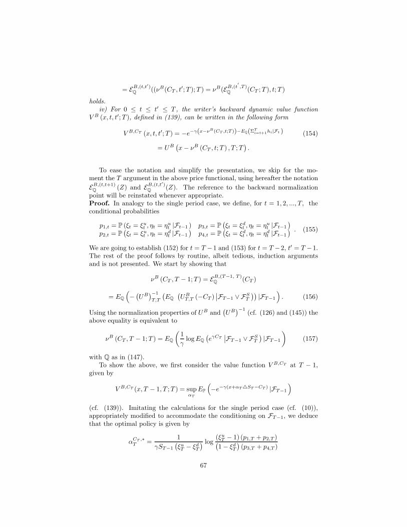
= EB,(t,t′)Q ((νB(CT , t′; T ); T ) = νB(E

B,(t′

,T )Q (CT ; T ), t; T )

holds.iv) For 0 ≤ t ≤ t′ ≤ T , the writer’s backward dynamic value function

V B (x, t, t′; T ), defined in (139), can be written in the following form

V B,CT (x, t, t′; T ) = −e−γ(x−νB(CT ,t;T ))−EQ(ΣTi=t+1hi|Ft ) (154)

= UB(x − νB (CT , t; T ) , T ; T

).

To ease the notation and simplify the presentation, we skip for the mo-ment the T argument in the above price functional, using hereafter the notation

EB,(t,t+1)Q (Z) and E

B,(t,t′)Q (Z). The reference to the backward normalization

point will be reinstated whenever appropriate.Proof. In analogy to the single period case, we define, for t = 1, 2, ..., T, theconditional probabilities

p1,t = P (ξt = ξut , ηt = ηu

t |Ft−1 ) p3,t = P(ξt = ξd

t , ηt = ηut |Ft−1

)

p2,t = P(ξt = ξu

t , ηt = ηdt |Ft−1

)p4,t = P

(ξt = ξd

t , ηt = ηdt |Ft−1

) . (155)

We are going to establish (152) for t = T −1 and (153) for t = T −2, t′ = T −1.The rest of the proof follows by routine, albeit tedious, induction argumentsand is not presented. We start by showing that

νB (CT , T − 1; T ) = EB,(T−1, T )Q (CT )

= EQ

(−(UB)−1

T,T

(EQ

(UB

T,T (−CT )∣∣FT−1 ∨ FS

T

))|FT−1

). (156)

Using the normalization properties of UB and(UB)−1

(cf. (126) and (145)) theabove equality is equivalent to

νB (CT , T − 1; T ) = EQ

(1

γlog EQ

(eγCT

∣∣FT−1 ∨ FST

)|FT−1

)(157)

with Q as in (147).To show the above, we first consider the value function V B,CT at T − 1,

given by

V B,CT (x, T − 1, T ; T ) = supαT

EP

(−e−γ(x+αT ST−CT ) |FT−1

)

(cf. (139)). Imitating the calculations for the single period case (cf. (10)),appropriately modified to accommodate the conditioning on FT−1, we deducethat the optimal policy is given by

αCT ,∗T =

1

γST−1

(ξuT − ξd

T

) log(ξu

T − 1) (p1,T + p2,T )(1 − ξd

T

)(p3,T + p4,T )

67

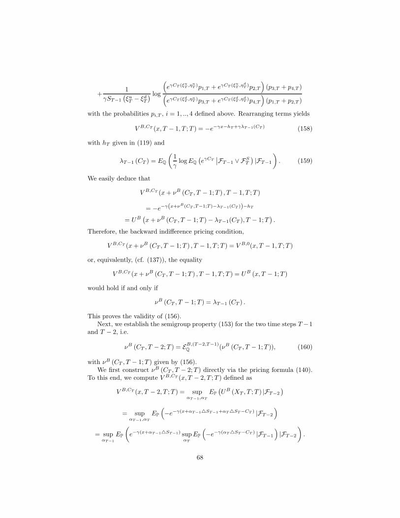
+1

γST−1

(ξuT − ξd

T

) log

(eγCT (ξu

T ,ηuT )p1,T + eγCT (ξu

T ,ηdT )p2,T

)(p3,T + p4,T )

(eγCT (ξd

T ,ηuT )p3,T + eγCT (ξd

T ,ηdT )p4,T

)(p1,T + p2,T )

with the probabilities pi,T , i = 1, .., 4 defined above. Rearranging terms yields

V B,CT (x, T − 1, T ; T ) = −e−γx−hT +γλT−1(CT ) (158)

with hT given in (119) and

λT−1 (CT ) = EQ

(1

γlog EQ

(eγCT

∣∣FT−1 ∨ FST

)|FT−1

). (159)

We easily deduce that

V B,CT (x + νB (CT , T − 1; T ) , T − 1, T ; T )

= −e−γ(x+νB(CT ,T−1;T )−λT−1(CT ))−hT

= UB(x + νB (CT , T − 1; T ) − λT−1(CT ), T − 1; T

).

Therefore, the backward indifference pricing condition,

V B,CT (x + νB (CT , T − 1; T ) , T − 1, T ; T ) = V B,0(x, T − 1, T ; T )

or, equivalently, (cf. (137)), the equality

V B,CT (x + νB (CT , T − 1; T ) , T − 1, T ; T ) = UB (x, T − 1; T )

would hold if and only if

νB (CT , T − 1; T ) = λT−1 (CT ) .

This proves the validity of (156).Next, we establish the semigroup property (153) for the two time steps T −1

and T − 2, i.e.

νB (CT , T − 2; T ) = EB,(T−2,T−1)Q (νB (CT , T − 1; T )), (160)

with νB (CT , T − 1; T ) given by (156).We first construct νB (CT , T − 2; T ) directly via the pricing formula (140).

To this end, we compute V B,CT (x, T − 2, T ; T ) defined as

V B,CT (x, T − 2, T ; T ) = supαT−1,αT

EP

(UB (XT , T ; T ) |FT−2

)

= supαT−1,αT

EP

(−e−γ(x+αT−1ST−1+αT ST−CT ) |FT−2

)

= supαT−1

EP

(e−γ(x+αT−1ST−1) sup

αT

EP

(−e−γ(αT ST−CT ) |FT−1

)|FT−2

).

68

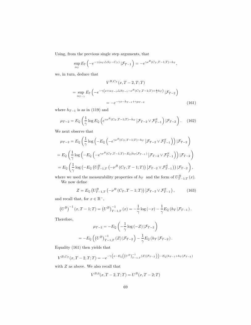
Using, from the previous single step arguments, that

supαT

EP

(−e−γ(αT ST−CT ) |FT−1

)= −eγνB(CT ,T−1;T )−hT ,

we, in turn, deduce that

V B,CT (x, T − 2, T ; T )

= supαT−1

EP

(−e−γ(x+αT−1ST−1−νB(CT ,T−1;T )+ 1

γhT ) |FT−2

)

= −e−γx−hT−1+γµT−2 (161)

where hT−1 is as in (119) and

µT−2 = EQ

(1

γlog EQ

(eγνB(CT ,T−1;T )−hT

∣∣FT−2 ∨ FST−1

)|FT−2

). (162)

We next observe that

µT−2 = EQ

(1

γlog(−EQ

(−eγνB(CT ,T−1;T )−hT

∣∣FT−2 ∨ FST−1

))|FT−2

)

= EQ

(1

γlog(−EQ

(−eγνB(CT ,T−1;T )−EQ(hT |FT−1 )

∣∣FT−2 ∨ FST−1

))|FT−2

)

= EQ

(1

γlog(−EQ

(UB

T−1,T

(−νB (CT , T − 1; T )

) ∣∣FT−2 ∨ FST−1

))|FT−2

),

where we used the measurability properties of hT and the form of UBT−1;T (x).

We now define

Z = EQ

(UB

T−1,T

(−νB (CT , T − 1; T )

) ∣∣FT−2 ∨ FST−1

), (163)

and recall that, for x ∈ R−,

(UB)−1

(x, T − 1; T ) =(UB)−1

T−1,T(x) = −

1

γlog (−x) −

1

γEQ (hT |FT−1 ) .

Therefore,

µT−2 = −EQ

(−

1

γlog (−Z) |FT−2

)

= −EQ

((UB)−1

T−1,T(Z) |FT−2

)−

1

γEQ (hT |FT−2 ) .

Equality (161) then yields that

V B,CT (x, T − 2, T ; T ) = −e−γ

“

x−EQ

“

(UB)−1

T−1,T(Z)|FT−2

””

−EQ(hT−1+hT |FT−2 )

with Z as above. We also recall that

V B,0(x, T − 2, T ; T ) = UB(x, T − 2; T )

69

= −e−γx−EQ(hT−1+hT |FT−2 ).

Combining the above yields that

V B,CT (x + νB (CT , T − 2; T ) , T − 2, T ; T ) = V B,0(x, T − 2, T ; T ),

if only if

νB (CT , T − 2; T ) = EQ

(−(UB)−1

T−1;T(Z) |FT−2

)

or, by using (163), if and only if

νB (CT , T − 2; T ) = EB,(T−2,T−1)Q

(νB (CT , T − 1; T ) ; T

)

= EQ

(−(UB)−1

T−1,T

(EQ

(UB

T−1,T

(−νB (CT , T − 1; T )

) ∣∣FT−2 ∨ FST−1

))|FT−2

)

and the assertion follows.The claimed measurability property of the backward price, νB(CT , t; T ) ∈

Ft, and the representation (154) of the backward dynamic value function followeasily.

Note that even though hT ∈ FT−1, it may fail to be FST−1-measurable. As

a consequence, for the auxiliary quantity µT−2, used above to establish thesemigroup property, we have

µT−2 = EQ

(1

γlog EQ

(eγνB(CT ,T−1;T )−hT

∣∣FT−2 ∨ FST−1

)|FT−2

)

6= EQ

(−

1

γhT +

1

γlog(EQ

(eγνB(CT ,T−1;T )

∣∣FT−2 ∨ FST−1

))|FT−2

).

On the other hand, we showed that

µT−2 = EQ

(−

1

γhT |FT−2

)

−EQ

((UB)−1

T−1;T

(EQ

(UB

T−1,T

(−νB (CT , T − 1; T )

) ∣∣FT−2 ∨ FST−1

))|FT−2

).

Comparing the above we see that, in general,

−EQ

((UB)−1

T−1,T

(EQ

(UB

T−1,T

(−νB (CT , T − 1; T )

) ∣∣FT−2 ∨ FST−1

))|FT−2

)

6= EQ

(1

γlog EQ

(eγνB(CT ,T−1;T )

∣∣FT−2 ∨ FST−1

)|FT−2

). (164)

While at this point, this might look like a technical nuisance, it will turn outthat (164) has very important consequences on the nature of the backward and

70

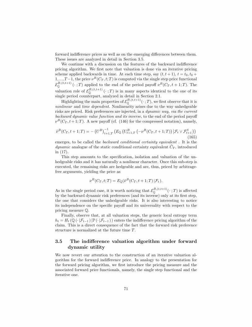
forward indifference prices as well as on the emerging differences between them.These issues are analyzed in detail in Section 3.5.

We continue with a discussion on the features of the backward indifferencepricing algorithm. We first note that valuation is done via an iterative pricingscheme applied backwards in time. At each time step, say (t, t + 1), t = t0, t0 +1, ..., T−1, the price νB(CT , t; T ) is computed via the single step price functional

EB,(t,t+1)Q (· ; T ) applied to the end of the period payoff νB(CT , t + 1; T ). The

valuation role of EB,(t,t+1)Q (· ; T ) is in many aspects identical to the one of its

single period counterpart, analyzed in detail in Section 2.1.

Highlighting the main properties of EB,(t,t+1)Q (· ; T ), we first observe that it is

nonlinear and time dependent. Nonlinearity arises due to the way unhedgeablerisks are priced. Risk preferences are injected, in a dynamic way, via the currentbackward dynamic value function and its inverse, to the end of the period payoffνB(CT , t+1; T ). A new payoff (cf. (146) for the compressed notation), namely,

νB(CT , t + 1; T ) = −(UB)−1

t+1,T

(EQ

(UB

t+1,T

(−νB(CT , t + 1; T )

) ∣∣Ft ∨ FSt+1

))

(165)emerges, to be called the backward conditional certainty equivalent . It is thedynamic analogue of the static conditional certainty equivalent CT , introducedin (17).

This step amounts to the specification, isolation and valuation of the un-hedgeable risks and it has naturally a nonlinear character. Once this sub-step isexecuted, the remaining risks are hedgeable and are, thus, priced by arbitrage-free arguments, yielding the price as

νB(CT , t; T ) = EQ(νB(CT , t + 1; T ) |Ft ).

As in the single period case, it is worth noticing that EB,(t,t+1)Q (· ; T ) is affected

by the backward dynamic risk preferences (and its inverse) only at its first step,the one that considers the unhedgeable risks. It is also interesting to noticeits independence on the specific payoff and its universality with respect to thepricing measure Q.

Finally, observe that, at all valuation steps, the generic local entropy termht = Ht (Q (· |Ft−1 ) |P (· |Ft−1 ) ) enters the indifference pricing algorithm of theclaim. This is a direct consequence of the fact that the forward risk preferencestructure is normalized at the future time T .

3.5 The indifference valuation algorithm under forward

dynamic utility

We now revert our attention to the construction of an iterative valuation al-gorithm for the forward indifference price. In analogy to the presentation forthe forward pricing algorithm, we first introduce the pricing measure and theassociated forward price functionals, namely, the single step functional and theiterative one.

71

The forward normalization point is taken to be s and is assumed to besmaller than the occurrence time of the cash flow. In the definition of theforward price functionals, the forward dynamic utility UF (x, t; s) and its inverse(UF)−1

(x, t; s) appear. The inverse forward dynamic utility(UF)−1

: R− ×[0, T ] is defined with respect to the wealth argument and is given, for t ≥ s, by

(UF)−1

(x, t; s) = −1

γlog (−x) −

1

γ

t∑

i=s+1

hi. (166)

To simplify the presentation we will occasionally use the compressed notation

UF (x, t; s) = UFs,t (x) and

(UF)−1

(x, t; s) =(UF)−1

s,t(x) for t ≥ s,

(167)whenever appropriate. Note that in contrast to the compressed backward no-tation (146), the point s, at which the forward dynamic utility is normalized,precedes the valuation time t.

Definition 58 Let Z be a random variable on (Ω,F , P) and Ft and FSt be

the previously introduced filtrations. Let s be the forward normalization point

and UFs,t (x) and

(UF)−1

s,t(x) be, respectively, the forward dynamic utility and its

inverse. We define:i) the pricing measure Q to be a martingale measure with the minimal relative

to P entropy, that is, satisfying, for t = 0, 1, ...

Q(ηt+1

∣∣Ft ∨ FSt+1

)= P

(ηt+1

∣∣Ft ∨ FSt+1

), (168)

ii) the single step forward price functional

EF,(t,t+1)Q (Z; s) = EQ

(−(UF)−1

s,t+1

(EQ

(UF

s,t+1 (−Z)∣∣Ft ∨ FS

t+1

))|Ft

),

(169)and

iii) the iterative forward price functional

EF,(t,t′)Q (Z; s) = E

F,(t,t+1)Q (E

F,(t+1,t+2)Q (...(E

F,(t′−1,t′)Q (Z; s))); s) (170)

across the time interval (t, t′).

As in the backward case, we caution the reader that, in general, for t′ 6= t+1,

EF,(t,t′)Q (Z; s) 6= EQ

(−(UF)−1

s,t′

(EQ

(UF

s,t′ (−Z)∣∣Ft ∨ FS

t′))

|Ft

). (171)

We are now ready to present a multi-period iterative valuation algorithmfor the calculation of the indifference prices under the fowrad dynamic utilityUF (x, t; s). The claim in consideration is introduced at t0 and offers a singlecash flow Ct ∈ Ft at time t. It is assumed that the forward normalization points satisfies s ≤ t0 < t. We are interested in the development of a scheme for theforward indifference price calculation at intermediate times t, with t0 ≤ t ≤ t.

72

Theorem 59 Let Ct ∈ Ft be the claim, introduced at t0 and to be priced underthe forward utility UF (x, t; s). The following statements are true:

i) The forward indifference price νF (Ct, t; s), defined in (143), is given, fort0 ≤ t ≤ t, by the algorithm

νF (Ct, t; s) = EF,(t,t+1)Q (νF (Ct, t + 1; s); s), νF (Ct, t; s) = Ct, (172)

with EF,(t,t+1)Q (· ; s) and Q defined respectively by (169) and (168).

ii) The forward indifference price process νs(Ct, t; s) ∈ Ft and satisfies

νF (Ct, t; s) = EF,(t,t)Q (Ct; s), t ≥ t0, (173)

with the iterative forward price functional defined in (170).iii) The forward pricing algorithm is consistent across time in that, for s ≤

t ≤ t′ ≤ t, the semigroup property

νF (Ct, t; s) = EF,(t,t′)Q (E

F,(t′

,t)Q (Ct; s) ; s) (174)

= EF,(t,t′)Q (νF (Ct, t

′; s); s) = νF (EF,(t

′

,t)Q (Ct; s), t; s)

holds.iv) For s ≤ t0 ≤ t ≤ t′ ≤ t, the writer’s forward dynamic value function

V F,Ct (x, t, t′; s), defined in (142), can be written in the following forms

V F,Ct (x, t, t′; s) = −e−γ(x−νF (Ct,t;s))+Σti=s+1hi (175)

= UF(x − νF (Ct, t; s) , t; s

).

Before we present the proof of the above Theorem, we present the followingLemma.

Lemma 60 Let Z be a random variable on the probability space (Ω,F , P). Let

also s be the forward normalization point and UF and(UF)−1

be, respectively,

the forward dynamic utility and its inverse. If EF,(t,t+1)Q (; s) is the single step

forward price functional, introduced in (169), then, for all t ≥ s,

EF,(t,t+1)Q (Z ; s) = EQ

(1

γlog(EQ

(eγZ

∣∣Ft ∨ FSt+1

))|Ft

). (176)

Proof. We recall that the local entropy terms hi ∈ Fi−1 for i ≥ 1. Therefore,t+1∑

i=s+1

hi ∈ Ft. Calculating, at the generic argument Z, the single step forward

price functional yields

EF,(t,t+1)Q (Z; s) = EQ

(−(UF)−1

s,t+1

(EQ

(UF

s,t+1 (−Z)∣∣Ft ∨ FS

t+1

))|Ft

)

73

= EQ

(1

γlog(−(EQ

(UF

s,t+1 (−Z)∣∣Ft ∨ FS

t+1

)))+

1

γ

t+1∑

i=s+1

hi |Ft

)

=1

γ

t+1∑

i=s+1

hi + EQ

(1

γlog(EQ

(eγZ−Σt+1

i=s+1hi∣∣Ft ∨ FS

t+1

))|Ft

)

=1

γ

t+1∑

i=s+1

hi + EQ

(1

γlog(EQ

(eγZ

∣∣Ft ∨ FSt+1

))|Ft

)−

1

γ

t+1∑

i=s+1

hi

and the statement follows.

We continue with the proof of the above Theorem. Since the technicalarguments are similar to the ones used for the construction of the backwarditerative algorithm (see proof of Theorem 57), we only present the main steps.Proof. We start by showing that

νF (Ct, t − 1; s) = EF,(t−1,t)Q (Ct; s)

= EQ

(−(UF)−1

s,t

(EQ

(UF

s,t (−Ct)∣∣Ft−1 ∨ FS

t

))|Ft−1

)

or, equivalently, that

νF (Ct, t − 1; s) = EQ

(1

γlog EQ

(eγCt

∣∣Ft−1 ∨ FSt

)|Ft−1

)(177)

with Q as in (168). To prove the above, we first consider the spot value functionV F,Ct at t − 1, given by

V F,Ct(x, t − 1, t; s) = supαt

EP

(UF (Xt − Ct, t; s) |Ft−1

).

We easily deduce that

V F,Ct(x, t − 1, t; s) = supαt

EP

(−e−γ(x+αtSt−Ct)+Σt

i=s+1hi |Ft−1

)

= −e−γx+Σt−1i=s+1hi sup

αt

EP

(−e−γ(αtSt−Ct)+ht |Ft−1

),

where we used the measurability properties of the local entropy terms. Imitatingthe calculations for the single period case (cf. (14)), appropriately modified toaccommodate the conditioning on Ft−1, we deduce that

V F,Ct(x, t − 1, t; s) = −e−γx+Σt−1i=s+1hi+γλt−1(Ct)

with

λt−1 (Ct) = EQ

(1

γlog EQ

(eγCt

∣∣Ft−1 ∨ FSt

)|Ft−1

).

74

It is then immediate that the pricing condition

V F,Ct(x + νF (Ct, t − 1; s) , t − 1, t; s) = V F,0(x, t − 1, t; s)

or, equivalently, due to (cf. (138)), the equality

−e−γ(x+νF (Ct,t−1;s))+Σt−1i=s+1hi+γλt−1(Ct) = −e−γx+Σt−1

i=s+1hi

would hold if and only if

νF (Ct, t − 1; s) = λt−1 (Ct) .

This proves the validity of (177).Next, we establish the semigroup property (174) for the two time steps t− 1

and t − 2, i.e. that

νF (Ct, t − 2; s) = EF,(t−2,t−1)Q (νF (Ct, t − 1; s) ; s),

or, equivalently,

νF (Ct, t − 2; s) = EQ

(1

γlog EQ

(eγνF (Ct,t−1;s)

∣∣Ft−2 ∨ FSt−1

)|Ft−2

)(178)

with νF (Ct, t − 1; s) as in (177).We first construct νF (Ct, t − 2; s) directly via the pricing formula (143). To

this end, we start with the computation of V F,Ct(x, t − 2, t; s). From (142) wehave,

V F,Ct(x, t − 2, t; s) = supαt−1,αt

EP

(UF (Xt, t; s) |Ft−2

)

= supαt−1,αt

EP

(−e−γ(x+αt−1St−1+αtSt−Ct)+Σt

i=s+1hi |Ft−2

).

Further calculations, together with the fact that

supαt

EP

(−e−γ(αtSt−Ct−

1γ

ht) |Ft−1

)= −eγνF (Ct,t−1;s),

yieldV F,Ct(x, t − 2, t; s)

= e−γx+Σt−2i=s+1hi sup

αt−1

EP

(−e−γ(αt−1St−1−νF (Ct,t−1;s)− 1

γht−1) |Ft−2

)

with νF (Ct, t − 1; s) as in (177). We then easily conclude that

V F,Ct(x, t − 2, t; s) = −e−γx+Σt−2i=s+1hi+γλt−2

where

λt−2 = EQ

(1

γlog EQ

(eγνF (Ct,t−1;s)

∣∣Ft−2 ∨ FSt−1

)|Ft−2

).

75

From the forward pricing condition (143) and the above equalities, it is thenimmediate that the pricing condition

V F,Ct(x + νs (Ct, t − 2; s) , t − 2, t; s) = V F,0(x, t − 2, t; s)

will hold if and only ifνF (Ct, t − 2; s) = λt−2,

and assertion (178) follows.The claimed measurability property of the forward price, νF (Ct, t; s) ∈ Ft,

and the representation (175) of the forward dynamic value function follow easily.

As in the backward case, the forward indifference valuation is done via aniterative pricing scheme applied backwards in time. At each time step, say(t, t + 1), with t0 ≤ t ≤ t − 1, the price νF (Ct, t; s) is computed via the single

step forward price functional EF,(t,t+1)Q applied to the end of the period pay-

off νF (Ct, t + 1; s). The valuation role of EF,(t,t+1)Q is similar to its backward

counterpart in that it nonlinear and time dependent.The forward dynamic risk preferences are injected via the current forward

dynamic value function and its inverse to the end of the period payoff νF (Ct, t+1; s). The new payoff (cf. (167) for the compressed notation)

νF (Ct, t + 1; s) = −(UF)−1

s,t+1

(EQ

(UF

s,t+1

(−νF (Ct, t + 1; s)

) ∣∣Ft ∨ FSt+1

))

= EQ

(1

γlog(EQ

(eγνF (Ct,t+1;s)

∣∣Ft ∨ FSt+1

))|Ft

)(179)

emerges, to be called the forward conditional certainty equivalent. It is thedynamic analogue of the static conditional certainty equivalent CT (cf. (17))and, also, the forward analogue of the backward conditional certainty equivalentνB(CT , t + 1; T ) (cf. (165)). Naturally, it is of nonlinear character since it is atthis valuation step that the unhedgeable risks are identified and priced.

Once this sub-step is executed, the remaining risks are hedgeable and are,thus, priced by arbitrage-free arguments, yielding the forward price as

νF (Ct, t; s) = EQ(νF (Ct, t + 1; s) |Ft ).

As in the single-period and forward cases, EF,(t,t+1)Q (· ; s) is affected by the

forward risk preferences (and its inverse) only at its first step, the one thatconsiders the unhedgeable risks. It is independent on the specific payoff and ituses the same pricing measure Q through all time steps.

Finally, it is important to observe that the same pricing measure Q appears inboth backward and forward valuational functionals even though the associatedrisk preferences are of very different nature.

Note, however, that there is a fundamental difference in the way marketincompleteness appears in the backward and in the forward indifference valuationalgorithms.

76

To elaborate, let us first recall that the single-step backward and forwardfunctionals are given, respectively, by

EB,(t,t+1)Q (ZB; T ) = EQ

(−(UB)−1

t+1,T

(EQ

(UB

t+1,T

(−ZB

) ∣∣Ft ∨ FSt+1

))|Ft

)

and

EF,(t,t+1)Q (ZF ; s) = EQ

(−(UF)−1

s,t+1

(EQ

(UF

s,t+1

(−ZF

) ∣∣Ft ∨ FSt+1

))|Ft

),

where T and s are the backward and forward normalization points, and UBt+1,T ,

UFs,t+1 and

(UB

t+1,T

)−1,(UF

s,t+1

)−1the backward and forward dynamic utilities

and their inverses. The variables ZB and ZF play the role of the end of theperiod backward and forward local payoffs.

Recalling the definition of UBt+1,T (and its inverse) we see that, in every step

(t, t + 1), the local entropy ht+1 enters in EB,(t,t+1)Q (· ; T ), via the backward

dynamic preferences. It is important to notice that these entropic terms areindependent of the specific claim and change dynamically in time. Moreover,the single step backward price functional depends on the normalization point,and hence so does the backward indifference price.

On the other hand, as it is stated in the above Lemma, the single step forward

price functional EF,(t,t+1)Q (· ; s) is essentially time invariant with regards to the

local in time changes of the forward dynamic risk preferences. This propertystrongly indicates that the forward dynamic utility measures utility across timesin a more intuitive fashion. Indeed, it is time invariant and model independentfor the next time period. However, further it looks ahead in the future, the moreinformation it incorporates about the degree of market incompleteness throughthe local entropic terms. These successive entropic terms give an idea of excessreturn locally in time and along the path. The forward dynamic utility doesnot provide such refined information since it only aggregates the entropies andincorporates their estimate.

Finally, as evidenced by (176), the functional EF,(t,t+1)Q (· ; s) is independent

on the normalization point s and hence so is the forward indifference price

νF (Ct, t; s). As a consequence, from now on, we will use the notation EF,(t,t+1)Q (·

) and νF (Ct, t) for the single step forward price functional and the forwardindifference price of Ct, calculated at time t.

3.6 A reduced binomial model and its backward and for-

ward prices

The discussion at the end of the previous section sheds light to the differentway the backward and forward dynamic preferences incorporate information onmarket incompleteness and how, in turn, the two algorithms process it. Due tothe distinct nature of backward and forward preferences and valuation schemes,it is therefore natural to expect that the backward and forward indifferenceprices do not, in general, coincide.

77

Naturally, such differences should dissipate when the market becomes com-plete and the indifference prices converge to the arbitrage-free ones. If the mar-ket remains incomplete, however, an important question arises, related to whenthe backward and forward indifference prices coincide across times. This clearlypoints to a relationship between the model definition and the specification ofthe dynamic preference structure.

To gain some intuition for the upcoming result, let us review the main stepsin the construction of the backward price algorithm. Referring to the proof ofTheorem 57, and specifically to the remark following it, we recall that, at each

valuation step, the single step backward price functional EB,(t,t+1)Q (· ; T ) acts on

two emerging terms, namely, the local entropy term, ht+1, and the local payoffνB (CT ; t + 1; T ).

As it was mentioned earlier, while ht+1 is always Ft−measurable, it may failto be FS

t −measurable for arbitrary incomplete binomial models. Therefore, the

additive invariance property (cf. Proposition 11) of EB,(t,t+1)Q (· ; T ) cannot be

applied and ht+1 does not scale out.The above observation clearly indicates that discrepancies between prices

could be remedied if additional conditions are imposed on the model resultingin the entropy terms ht+1 to be FS

t −measurable, for all t ∈ [0, T ]. This isformulated in the upcoming condition (180). In this case, as the proof belowshows, the backward and forward price functionals produce, at each time step,the same outcome which ultimately yields identical prices under the two kindsof preferences (cf. (181)).

Lemma 61 Assume that for all t ∈ [0, T ],

P(ξt+1 = ξu

t+1 |Ft

)= P

(ξt+1 = ξu

t+1

∣∣FSt

). (180)

Then the local entropy terms, defined in (119), satisfy ht ∈ FSt−1, for 0 ≤ t ≤ T.

The proof of the above Lemma follows from the definition of ht and it isomitted.

We next introduce a binomial model similar to the one introduced in Section3.1 but with the additional assumption (180) on the transition probabilities ofthe traded asset. This is the same setting considered by the authors in Musielaand Zariphopoulou (2004b) as well as in Smith and Nau (1995), Becherer (2002),and Elliott and Van der Hoek herein. We will refer to this model as the reducedbinomial model.

Proposition 62 Consider the reduced binomial model introduced above. As-sume dynamic risk references of backward and forward kind with respective nor-malization points s and T , 0 ≤ s < T . Consider a claim that yields a single

cash flow CT ∈ FT . Let νB and νF be its backward and forward indifferenceprices. Then, for all CT and t ≤ T the two prices coincide, namely,

νB (CT , t; T ) = νF (CT , t) . (181)

78

Proof. We first observe, from (157) and (177), that

νB (CT , T − 1; T ) = νF (CT , T − 1)

= EQ

(1

γlog(EQ

(eγCT

∣∣FT−1 ∨ FST

))|FT−1

).

We are going to establish (181) for t = T − 2, namely,

νB (CT , T − 2; T ) = νF (CT , T − 2) .

Recall (cf. (178)) that

νF (CT , T − 2) = EQ

(1

γlog(EQ

(eγνF (CT ,T−1)

∣∣FT−2 ∨ FST−1

))|FT−2

).

Combining the above, we deduce that it suffices to show

νB (CT , T − 2; T ) = EQ

(1

γlog(EQ

(eγνB(CT ,T−1;T )

∣∣FT−2 ∨ FST−1

))|FT−2

).

From Theorem 57, we obtain

νB (CT , T − 2; T ) = EB,(T−2,T−1)Q

(νB (CT , T − 1; T ) ; T

)

= EQ

(−(UB)−1

T−1,T

(EQ

(UB

T−1,T

(−νB (CT , T − 1; T )

) ∣∣FT−2 ∨ FST−1

))|FT−2

).

Note, however, that because hT ∈ FST−1,

EQ

(UB

T−1,T

(−νB (CT , T − 1; T )

) ∣∣FT−2 ∨ FST−1

)

= EQ

(−eγνB(CT ,T−1;T )−EQ(hT |FT−1 )

∣∣FT−2 ∨ FST−1

)

= EQ

(−eγνB(CT ,T−1;T )−hT

∣∣FT−2 ∨ FST−1

)

= e−hT EQ

(−eγνB(CT ,T−1;T )

∣∣FT−2 ∨ FST−1

).

Therefore,

EQ

(−(UB)−1

T−1,T

(EQ

(UB

T−1,T

(−νB (CT , T − 1; T )

) ∣∣FT−2 ∨ FST−1

))|FT−2

)

= EQ

(−(UB)−1

T−1,T

(e−hT EQ

(−eγνB(CT ,T−1;T )

∣∣FT−2 ∨ FST−1

))|FT−2

)

= EQ

(1

γlog(−e−hT EQ

(−eγνB(CT ,T−1;T )

∣∣FT−2 ∨ FST−1

))+

1

γhT |FT−2

)

= EQ

(−

1

γhT +

1

γlog EQ

(eγνB(CT ,T−1;T )

∣∣FT−2 ∨ FST−1

)+

1

γhT |FT−2

)

= EQ

(1

γlog(EQ

(eγνB(CT ,T−1;T )

∣∣FT−2 ∨ FST−1

))|FT−2

)

and the result follows.To conclude, we need to show that equality (181) holds for t = T−3, T−4, ..s.

The involved arguments can be easily reproduced in an inductive manner andare not presented.

79

4 Bibliography

Artzner P., Delbaen F., Eber J.-M. and Heath D., Coherent measures of risk,Mathematical Finance 9 (3), 203–228 (1999).

Artzner P., Delbaen F., Eber J.-M. and Heath D., Multi-period risk andcoherent mult-iperiod risk measurement, preprint (2003).

Becherer, D.: Rational hedging and valuation of integrated risks under con-stant absolute risk aversion, preprint (2002).

Delbaen, F., Grandits, P., Rheinlander, T., Samperi, D., Schweizer, M.,Stricker, C.: Exponential hedging and entropic penalties, Mathematical Finance,12 (2), 99–123 (2002).

Foellmer, H. and Schied, A.: Convex measures of risk and trading con-straints, Finance and Stochastics, 6, 429–447 (2002a).

Foellmer, H. and Schied, A.: Robust preferences and convex measures ofrisk, Advances in Finance and Stochastics, Springer, Berlin, (2002b).

Frittelli, M.: The minimal entropy martingale measure and the valuationproblem in incomplete markets, Mathematical Finance, 10, 39–52 (2000a).

Frittelli, M.: Introduction to a theory of value coherent with the no-arbitrageprinciple, Finance and Stochastics, 4, 275–297 (2000b).

Kabanov, Y. and Stricker, C.: On the optimal portfolio of exponential utilitymaximization: Remarks to the six-author paper, Mathematical Finance, 12 (2),125–134 (2002).

Merton, R.: Optimum consumption and portfolio rules in a continuous timemodel, Journal of Economic Theory, 3, 373–413, (1971).

Musiela, M. and Zariphopoulou, T.: Indifference prices and related measures,The University of Texas at Austin, Technical report, (2001a).

Musiela, M. and Zariphopoulou, T.: Pricing and Risk Management of deriva-tives written on non-traded assets, The University of Texas at Austin, Technicalreport, (2001b).

Musiela, M. and Zariphopoulou, T.: An example of indifference prices underexponential preferences, Finance and Stochastics, 8, 229–239, (2004a).

Musiela, M. and Zariphopoulou, T.: A valuation algorithm for indifferenceprices in incomplete markets, Finance and Stochastics, 8, 399–414 (2004b).

Musiela, M. and Zariphopoulou, T.: Forward indifference valuation in in-complete binomial models, preprint, (2005a).

Musiela, M. and Zariphopoulou, T.: Backward indifference valuation in in-complete binomial models, in preparation, (2005b).

Musiela, M., Zariphopoulou, T. and Zitkovic, G. : Numeraire consistencyand indifference valuation, in preparation (2005).

Rouge, R. and El Karoui, N.: Pricing via utility maximization and entropy,Mathematical Finance, 10, 259–276 (2000).

Smith, J., and McCardle, K.F.: Valuing oil properties: integrating optionpricing and decision analysis approaches, Operations Research, 46 (2), 198–217(1998).

Smith, J. and Nau, R.: Valuing risky projects: Option Pricing and DecisionsAnalysis, Management Science, 41 (5), 795–816, (1995).

80

Stoikov, S. F.: Option pricing from the point of view of a trader, submittedfor publication, (2005).

zariphop@math.utexas.edumarek.musiela@bnpparibas.com

81