Very preliminary

Do not cite

The Argentine Collapse:

Hard Money’s Soft Underbelly

Ricardo Hausmann

Andrés Velasco

Kennedy School of Government

Harvard University

April 26, 2002

I. Introduction

The Argentine crisis has been a humbling experience for policymakers,

investors, academics and more than a few op-ed writers. This was not an event that

caught people by surprise. Instead, it was a protracted affair that, as it marched

inexorably towards a catastrophic demise, garnered the attention of the best minds in

Washington, Wall Street and Buenos Aires for months on end.

The main actors of this drama, whether in Argentina or abroad, were well-

trained economists, deeply knowledgeable of previous crisis episodes and profoundly

aware of the lessons of the past and the policy implications of new theories. During

this long agony, many diagnostics were developed, many original and innovative

policy initiatives were tabled, much delegation of authority was provided by political

parties onto technocrats and significant international intellectual and financial support

was offered. And yet the catastrophe proved hard to sidestep.

This was not the first time that Argentina’s Convertibility had got into trouble.

During the Tequila crisis of 1995 the system had been tested by a massive collapse in

capital inflows and deposit demand. But Argentina came out roaring in 1996-1997

without any changes in its currency regime. Moreover, Argentine authorities used the

experience to lengthen the maturity of public debt, improve the liquidity of the

Treasury, upgrade banking regulation and create a path breaking liquidity policy that

assured the confidence of domestic agents and kept deposits growing throughout the

1998 recession and until as late as February 20011.

The theories that were present in the minds of actors in the Argentine crisis

spanned the whole scope of the academic literature. For some, the problem had a

fiscal origin and required a fiscal response (IMF, Lopez-Murphy, Mussa (2001)). In

such a context, a fiscal contraction could arguably become expansionary, since it

would eliminate fears of insolvency and make capital markets more forthcoming.

These ideas lead to a series of fiscal adjustment efforts that in fact increased the non-

social security primary surplus by over 2 percentage points of GDP in spite of the

1 For a description of Argentina’s banking reforms see Calomiris and Powell (2001)

recession2. They involved raising taxes, and by the summer of 2001, even cutting

nominal public sector wages, pensions and mandated inter-governmental federal

transfers.

For others, it was a multiple equilibria story, in which self-fulfilling

pessimism kept interest rates too high and growth too low for the numbers to add up.

Some pointed to liquidity concerns and rollover risks. In order to reassure the markets

and reestablish access, the government negotiated a 40 billion US$ lending package3

led by the IMF in November 2000, and negotiated a 30 billion dollar debt exchange in

May 2001. Neither had the expected effects.

In this same vein, some analysts blamed the pessimism of investors on the

lack of conviction of policymakers, and demanded a more forceful leader. This

concern lead to the return of Domingo Cavallo, the architect of the Convertibility

Plan of 2001 and allegedly a legend in the minds of Argentineans and market

participants alike. He demanded and was granted special powers to fix the economy

by decree The market reacted with a sharp rise in country risk.

Other students of the Argentine situation blamed the exchange rate, which had

moved in the wrong direction because of the dollar’s strength and the Real’s

weakness. Fearful of the balance sheet and credibility consequences of an exchange

rate move, the government in 2001 engineered a fiscal devaluation (i.e. a tariff for

imports accompanied by a subsidy for exports, leaving financial transaction and

hence balance-sheets untouched) of about 8 percent4. It accompanied this measure

with a planned gradual transition away from a pure US dollar basket and into a 50-50

dollar-euro peg. The markets reacted very negatively to this announcement.

2 As we shall see below, the de la Rúa administration started in January 2000 with a major fiscal adjustment– the impuestazo – that did not generate an expansionary contraction but instead was later blamed forhaving killed an incipient recovery in its bud. Three additional attempts at this strategy were made in 2001without any expansionary consequences.3 The program never added up to US$ 40 billion. This number included unidentified operations withmarkets for US$ 20 billion. The main component was a 14 billion US$ loan from the IMF and 5 billionfrom the IDB and World Bank. The latter amount was mainly previously planned lending and not much inadditional finance.4 This idea was originally proposed for Argentina by Calvo (1997). It is analyzed by Fernandez-Arias andTalvi (2000).

For others yet, the problem was growth and required a supply response. Here

again, a massive attempt was made at sectoral competitiveness plans. Markets again

remained unimpressed.

Finally, there have been many who blamed the Argentine crisis on political

gridlock. But this is also a hard case to make. In spite of an unrelenting recession and

with little to show for their efforts, the government consistently got from Congress an

unprecedented level of delegation of power. All major policy requests were granted:

labor market reforms, several tax increases, a special powers act in April 2001 and a

zero-deficit rule in the summer of 2001 that involved cutting wages and pensions and

making their recipients junior to bondholders. And yet, as in a Greek tragedy, destiny

proved unavoidable.

This paper tries to make sense of this sad experience. Section 2 discusses what

happened. Section 3 --entitled “what did not happen”-- analyzes the limitations of the

three major paradigms with which actors analyzed the unfolding crisis. Section 4

presents an analytical framework that tries to account for the crisis. It stresses the role

of an endogenous external financing constraint, and the limits this placed on domestic

investment and growth. With that framework we ask in section 5 what should have

happened, i.e. what were useful policy options the authorities could have pursued. We

find that fiscal contraction had very little chance of fixing things and that devaluation

alone could easily have made matters worse. By contrast, devaluations accompanied

by a pesification of financial claims could have resolved the crisis while minimizing

the loss to investors. We conclude in section 6 with some additional lessons and

policy conclusions.

II. What happened

Argentina collapsed into hyperinflation in the late 1980’s, but was able to

right itself by adopting a radical market-oriented reform anchored by a currency

board. The reforms delivered rapid growth in the early 90s, with a very rapid recovery

of investment (Table 1 and Figure 1). Then came the Tequila crisis in 1995,

characterized by a collapse in financial flows and investment that generated a deep

recession. Notice, however, that during the crisis exports skyrocketed, growing at real

rates in excess of 30 percent in 1995. The subsequent period of 1996 and 1997 saw

what appeared to be a very healthy export- and investment-lead growth. Concerns

over the competitiveness of the country were laid to rest as the economy was able to

extricate itself from the Tequila crisis and rebound back to high growth through

exports, without the disruptive devaluation that the Mexicans had undergone.

The East Asian crisis caused a fall in the terms of trade in the second semester

of 1997 (Figure 2). Then came the Russian crisis in August 1998 and later the

Brazilian devaluation of January 1999. Just as under the Tequila, output declined lead

by a collapse in investment. Would the economy turn itself around like the last time?

Notice that in this opportunity, export prices entered a severe slump, export volumes

lost their luster while investment continued to decline. The recovery never came. The

earlier magic was not repeated.

For much of the period after the Russian 1998 crisis in which the economy

was deteriorating, financial markets were persuaded that the situation was under

control. Until the Brazilian devaluation in January 1999, markets perceived Argentina

as just another Mexico. After that, while the risks were seen as somewhat larger,

Argentina’s country risk was well below that of Brazil, Venezuela or the EMBI+

average5 (Figure 3). It was only in the summer of 2001 that asset prices reflected an

ominous future.

Argentina obviously had a streak of bad luck. The terms of trade were

negatively impacted after the Asian crisis in the second semester of 1997. Financial

markets dried up after the Russian default in August 1998. Brazil abandoned its

crawling band and massively depreciated its currency in January 1999. The euro sank

by over 20 percent in 2000, further weakening Argentina’s competitiveness vis a vis

the important European market. The world entered into recession in 2001, not only

weakening commodity prices and export prospects, but creating additional turmoil in

financial markets associated with the bursting of the high tech bubble. Throw in

underwhelming new authorities in the US Treasury and the IMF and the implications

5 In fact, Argentina was seen as another Mexico until the Brazilian January 1999 devaluation. It wasperceived as a much safer bet than either Brazil or Venezuela until the first quarter of 2001.

of September 11 and you have the makings of a perfect storm. But Argentina had

already gone through a bad experience with the so-called Tequila crisis in 1995 and

came out roaring. Was it not just a question of keeping heads cool and policies

focused until the economy would turn around? That at least was the dominant view as

expressed by the IMF board in May 1999:

"Argentina is to be commended for its continued prudent policies.

As with a number of other countries in the region, Argentina has had to

bear the adverse consequences of external shocks, which have taken a

significant toll on economic performance. Nevertheless, the sound

macroeconomic management, the strengthening of the banking system and

the other structural reforms carried out in recent years in the context of the

currency board arrangement, have had beneficial effects on confidence,

and have allowed the country to deal with these challenges." IMF, News

Brief No. 99/24, May 26, 1999

III. What did not happen

As the drama unfolded, three major views developed as to the nature of the

problem and the appropriate policy response. The dominant view put the accent

firmly on self-fulfilling bad expectations. A second view – not completely unrelated –

emphasized problems of fiscal sustainability. Another view put the accent on

competitiveness and the rigidities of the exchange rate regime. As argued above, each

of these views was influential in policy circles and lead to important changes in the

policy framework.

Self-fulfilling pessimism

The self-fulfilling pessimism paradigm probably became dominant as it was seen as

the most convincing explanation of the 1995 Tequila crisis, which was associated

with a sudden and systemic collapse in capital inflows and in the demand for deposits

in the banking system. Without a lender of last resort, the country was vulnerable to

liquidity crises. To avoid future similar crises the authorities developed after the 1995

crisis a highly-praised liquidity policy which involved imposing high liquidity

requirements on banks, negotiating contingent credit lines with foreign banks,

lengthening the maturity of the public debt and keeping a liquid fiscal position. These

policies were handsomely rewarded by the markets through improved confidence and

market access. In fact, these policies together with the currency board were seen as

providing robust institutions to cope with financial turmoil6. They proved their mettle

during much of the subsequent crisis: deposits in the banking system kept growing

until February 2001.

With the banking system under control, self-fulfilling negative expectations

were seen as potentially originating from roll-over problems in the public debt. To

avoid such bad equilibria, the authorities negotiated a major expansion of

international official support in November 2000 – the so-called “blindaje”. They

repeated this strategy in the spring of 2001 with a 30 billion dollar debt exchange

designed to lengthen the maturity of debt coming due in the subsequent three years

and achieving a temporary reduction in interest payments.

Negative expectations were also seen as becoming self-fulfilling not just

through liquidity channels but also through fiscal conduits. Pessimism would lead to

high interest rates, which would depress growth and weaken the fiscal position,

complicating debt service and thus justifying the initial pessimism:

“Despite substantial efforts by the Argentine government to

implement the economic program it had announced in December

1999, and which the IMF has supported with a stand-by credit

since March 2000, economic performance in 2000 was worse than

expected. A major disappointment was the failure to recover from

the recession affecting economic activity since mid-1998. After a

short-lived pickup in the last quarter of 1999, the economy again

stagnated. This reflected in part the impact of the fiscal tightening

on domestic demand, but was mainly the result of a drop in

business and consumer confidence, and the progressive hardening

of financing conditions in international markets, that resulted in

6 “Argentina's convertibility regime and the liquidity defenses of the banking system are important pillarsof the country's economic strategy and have been vital in helping withstand turbulent financial conditions.The Fund, therefore, welcomes the authorities' reaffirmation of their commitment to these policies.” IMFPress Release No. 01/37 September 7, 2001.

rising borrowing costs and reduced market access for Argentine

private and official borrowers.” IMF, Press Release No. 01/3,

January 12, 2001

In designing a strategy to deal with the crisis the IMF program – revised in

May 2001- argued as follows:

"Argentina's program aims at strengthening confidence

through fiscal consolidation to achieve the program's targets for

2001 and fiscal balance by 2005, while promoting the recovery of

investment and output through fiscal incentives and regulatory

changes. Firm implementation of the program is needed to initiate

a virtuous circle of stronger public finances, lower interest rates,

and a recovery of economic activity. (italics added). IMF News

Brief No. 01/44 of May 21, 2001

To check some implications of this story we ran a simple simulation. We

assumed that enough “confidence” was reestablished to secure a 3 percent growth rate

starting in the fourth quarter of 1998. This simulation intends to illustrate a possible

counter-factual path, had the Russian crisis not affected the availability of finance and

a move towards a “bad” equilibrium. The simulation intends to use very crude

relationships, just to gauge the potential implications of alternative paths. We are not

taking account of other real shocks that the economy underwent throughout this

period.

To keep things simple, we include a minimum number of behavioral equations

but we keep the identities required by the national accounts. First, we incorporate the

impact of the higher output on a higher demand for imports. We calculate the

marginal propensity to import by running a regression between imports and output.

The estimated coefficient used for these simulations is .261. We also include the

higher external debt needed to run the wider current account deficit and we service

the additional accumulated debt in future years. We also take account of the impact of

the higher output on the primary balance. We calculate the marginal propensity to

save the additional fiscal revenues from the data by running a simple regression. The

estimated effect is 0.088. We leave all other fiscal variables as they are, except that

we count the impact of the lower path for public debt on the interest burden. We do

not include the potential impact of the higher domestic demand on a lower level of

exports, as this would only make our story even more compelling.

The simulations are presented if Figures 4 a, b, and c. As can be clearly seen,

the increased activity would have been enough to maintain the public debt to GDP

ratio relatively stable, below 40 percent of GDP instead of rising as it did up to almost

50 percent of GDP by the first quarter of 2001. However, in order to achieve this

path, the current account deficit would have had to average in excess of 6 percent of

GDP instead of declining to a 4 quarter moving average OF 3.1 percent of GDP by

the first quarter of 20017. This larger deficit implies that external obligations would

have had to rise by an additional 20 percent of GDP, even after correcting for the

larger denominator, given the higher growth. This implies an increase in the debt to

export ratio of about 200 percentage points.

Hence, leaving all other shocks aside, the “good equilibrium”, i.e. a

reestablishment of enough confidence to maintain growth at 3 percent would have

done away with the fiscal imbalance but would required the funding of sustained 6

percent current account deficits and the accumulation of an additional 20 percent of

GDP in external obligations. This assumes that external financial constraints would

not bind. As we shall see, if for some reason this amount of financing is not feasible,

then the good equilibrium would also not be feasible.

Fiscal sustainability

A second view of the crisis put the accent not so much on pessimism and

multiple equilibria, but on the more banal problem of fiscal solvency. After all, the

public debt went from 80.3 billion dollars at the end of 1994 to over 140 billion

7 Some would argue that if the fiscal adjustment had translated into a lower country risk, interest rates onnew debt would have declined, making the DEBT dynamics less unfavorable. However, much of the olddebt in Argentina was long term and had been contracted at rates well below those at which even countrieslike Mexico faced post-Russia. In the simulations we assume that the additional debt pays an 8 percentinterest, which is about 300 basis points over the US Treasury, a spread significantly below that of theaverage EMBI+, let alone the 700+ spread that Argentina faced during this period. Moreover, the bulk ofthe additional debt is explained by the trade deficit accumulated between the fourth quarter of 98 and thesecond quarter of 2001 (US$ 26.0 billion) and not to the additional interest payment (US$ 2.3 billion).

dollars in the summer of 2001. Is this not proof that the fiscal accounts were on an

unsustainable path? True, the fiscal problem had been aggravated by the recession,

but the debt had increased by 15 billion dollars in the three boom years of 1996-1998.

Was this not proof that the country could not enforce a budget constraint? (Mussa,

2002).

The importance of fiscal balance was present in the minds of the authorities

and the IMF throughout the slow evolving crisis. In fact, that was the diagnosis with

which Minister Jose Luis Machinea defined the economic situation in early 2000 in

order to justify his tax measures, the so-called impuestazo. It was also the

interpretation of Minister Ricardo Lopez Murphy who took office briefly in March

2001. When Minister Domingo Cavallo took over after him he immediately

implemented a financial transactions tax to improve the fiscal situation. He later

adopted the zero deficit policy in the summer of 2001.

The view that Argentina was somehow irresponsible in its fiscal management

and that this may have been a major cause of the crisis --and not just one of its

consequences-- has become a dominant story ex post. The idea that fiscal policy was

somehow inconsistent with the convertibility system has gained currency among

many analysts (References?) We do not share this view. As we shall see, the fiscal

imbalance was not large and was backed up by increased savings of the privatized

pensions system. Moreover, as the simulation above illustrates, the fiscal imbalance

that emerged was related to the recession and hence is best understood as a

consequence rather than a cause of the crisis. Moreover, as we will argue below, it is

very hard to make the case that a more forceful fiscal adjustment would have made a

very significant difference. In this section we will just present the facts in a way that

supports a rather different interpretation (Table 2)

The numbers quickly dispel any argument based on a spending feast.

Government spending remained remarkably flat as a share of GDP from 1993

onwards. If we exclude social security payments, other primary spending actually

declined by 1.5 percent of GDP (from 13.8 to 12.3 percent) during the pre-crisis

period 1993-1998.

It is important to understand the dynamics that were affecting the fiscal

accounts in Argentina. First, there was a rising interest burden of the debt. As shown

in Table 2 factor payments increased from 1.2 percent of GDP in 1993 to 3.4 percent

of GDP in 2000. This was due mainly to three factors:

• Some of the Brady Bonds issued during the early 1990s had rising interest

rates.

• The increase in the official public debt exceeded the accumulated deficit flows

between 1994 and 2000 by about 21 billion dollars, half of which was the

recognition of pre-existing debts and the rest represented the purchase of

financial assets (see the discussion in Table 4 below).

• After the Russian crisis, the country faced an interest rate on new debt which

was higher than the rate paid on average on the existing stock.

A second force affecting the fiscal accounts was the social security reform.

This caused revenues to the Social Security system to be diverted towards the new

privatized fund administrators. Social security revenues declined from 5.6 percent of

GDP in 1993 to 3.8 percent by 2000 (Table 2). This did not represent a reduction in

economy’s contributions to the system, only a change in the mechanism of allocation

and administration. By December 2000, the private pension fund administrators had

assets totaling 20.3 billion dollars8. By contrast, social security payments rose from

5.3 percent to 6.1 percent of GDP by 2000. This caused the social security balance to

swing from a surplus of 0.4 percent in 1993 – before the reform – to a deficit of 2.4

percent of GDP by 2000. The cumulative deficit of the social security component of

the budget between 1995 and 2000 was US$ 30.9 billion.

In order to confront these pressures on the budget, the authorities pursued a

policy of improving the primary surplus of the remaining parts of the budget, i.e.

excluding the social security system. This surplus increased from 1.3 percent of GDP

in 1995 to 3.3 percent in 2000. In this sense, the primary surplus achieved by

Argentina is perfectly comparable to that achieved by Brazil, a country that has not

privatized its social security system.

8 The assets of the AFJP are calculated at market prices, which were below their original purchase price.

Did the authorities really tighten fiscal policy when they found themselves in

trouble in 2000 or was it all just talk? Table 3 explores this issue by running

regressions of government revenues and primary spending with GDP and including a

dummy for the post-impuestazo period, i.e. the period starting in the second quarter of

2000. Several features can be highlighted. First, tax revenues show much more

buoyancy than spending. The estimated elasticity of tax revenues to GDP is 1.47,

while it is only 0.72 for primary spending excluding social security. This implies that

during the booming years of 1996 and 1997 government spending was kept subdued

relative to revenues9. By the same toke, the automatic reaction to the recession would

have implied a significant increase in the deficit. Second, revenues post the fiscal

adjustment in the first quarter of 2000 – the impuestazo – are estimated to have been

11 percent or 1 billion dollars per quarter higher than would have been expected

given GDP changes. By contrast, the dummy variable for spending is not statistically

significant, meaning the government was essentially just able to cut spending by the

expected amount, i.e. with an elasticity of 0.72 relative to the fall in GDP. This

explains in part the problems the government faced during the recession: revenues

would have fallen more than spending, but significant action was taken to prevent this

from happening and securing a continued improvement of the non-social-security

primary surplus.

Bringing it all together (Table 2 and Figure 5), it appears that one way to

describe the situation emanates quite naturally from the data: the government was

able to improve the (ex-social security) primary surplus to accommodate the increase

in debt service, while the overall deficit was essentially explained and in fact

somewhat smaller than the deficit of the social security system. However, the latter

was backed to a significant extent by the savings in the privatized pension system.

These calculations account for the published deficits. What about the assertion

that the growth of debt was out of control? Table 4 shows the increase in debt during

the 1995-2000 period. As can be seen, the total increase in debt of 42.7 billion

exceeds the cumulative deficit by 20.9 billion dollars. A bit over half of the difference

9 This fact is also clear in Figure 1 where government consumption appears as the least dynamic componentof aggregate demand during the boom periods. It does tend to show less downward adjustment in

is explained by the accumulation of assets (11.7 billion), while some 10.4 billion can

be explained by the recognition of pre-existing debts. Note that the cumulative overall

deficit is 10.1 billion dollars larger than the cumulative social security deficit, and is

equal to the accumulation of assets in the pension system.

In conclusion, fiscal policy was adjusted to generate a sufficient primary

surplus, (excluding the public social security system) in order to cover the increased

debt service. In fact the primary surplus was of the same magnitude as that of Brazil,

in spite of the deeper recession. The overall deficit was smaller than the deficit of the

social security system, which was backed up to a significant extent by saving flows

into the private pension funds. In addition, there was a significant accumulation of

assets and documentation of pre-existing debt.

Obviously, the country could have tried to run a tighter fiscal ship, but the

numbers here are not those of a profligate country are too parsimonious and thus hard

to square with the catastrophe that followed. Where is the dramatic shift in fiscal

outcomes between the time when Argentina was perceived as one of the safest

emerging markets (say, in 1999) and its eventual demise?

Exchange rate rigidity

The third influential theory was associated with the peculiar exchange rate

choice of Argentina. Faced with hyperinflation and in desperate need of a nominal

anchor, Argentina chose in 1991 a currency board with the dollar and a bi-monetary

financial system, one in which both the US dollar and the Argentine peso were legal

tender. The system achieved price stability, but left the country vulnerable to

inconvenient movements in the multilateral exchange rate. This possibility became a

reality after the Brazilian devaluation of January 1999 and the euro slide of 2000. The

story is clearly evident in the data (Figure 6).

It is clear that the nominal appreciation of the multilateral nominal exchange

rate (MNER) of Argentina took place at a most inconvenient time. The Brazilian

devaluation of 1999 had caused an appreciation of Argentina’s MNER of 14 percent.

Between January and July 2001, this exchange rate appreciated a further 13 percent.

recessions.

This was taking place against a backdrop of stagnant export volumes and low and

declining export prices, a development that would have required a movement in the

real exchange rate in the opposite direction. Hence, an increasing exchange rate

misalignment developed: the worsening external conditions called for a depreciated

equilibrium exchange rate, while the actual rate appreciated. Low and falling export

prices, a less competitive exchange rate and a rising cost of capital must have

wrecked havoc on the profitability of the export sector and thus on its ability to

expand supply. Export volume growth, which had averaged over 14 percent per year

between 1993 and September 1998, stalled and never again managed to recover its

earlier dynamism, in spite of the declining levels of domestic absorption (Table 1 and

Figure 2). And yet, it managed to maintain a 3.8 percent growth from the third quarter

of 1999 to the third quarter of 2001.

This standard logic can explain the protracted recession and the increasing

tension between the achievement of external balance and full employment. But why

would it lead to a financial crisis? As we showed in the simulations described in

Figures a, b and c, at the prevailing real exchange rate, even modest growth of 3

percent could only be achieved at the expense of large current account deficits and

rising debt ratios. Argentina thus found itself in a bind: if it tried to grow it risked

accumulating debt to the point of insolvency; if it chose to achieve external balance, it

would have had to achieve strongly negative growth rates, which would also have

imperiled its solvency.

Markets increasingly began to fear this latter risk, as shown in Figure 6. The

multilateral exchange rate tracked remarkably well the evolution of the spread

between the country risk of Argentina relative to that of Mexico, especially after the

Brazilian 1999 devaluation. We take Mexico as a benchmark since both economies

had very similar country risk spreads until the 1999. Both countries suffered a

common shock when emerging markets floundered after the Russian default, but after

the Brazilian devaluation, Argentina started to move in a different direction10.

10 Skeptics might wonder whether this correlation says anything about the perceived risk of exchange ratemisalignment. An alternative interpretation of Figure 1 is that both variables respond to a common drivingforce, namely Brazilian risk. Under this interpretation Argentine risk moves with Brazil’s because bothcountries are economically intertwined, while the multilateral exchange rate moves mainly because of

There is a clear sense then, in which Argentina did have an exchange rate

problem. What is much less clear, however, is whether it had an exchange rate

solution available to it. It was the combination of relative price misalignment with

increasingly scarce financing that made the situation vulnerable. And, with a large

accumulated dollar debt, both private and public, the competitiveness gains of a

potential devaluation had to be weighed against the balance sheet damage it would

inflict, and the additional market access this would bring. Putting these different

factors together, and trying to assess the policy tradeoffs involved, is what we try do

in the next section.

IV. What could have happened

If the conventional stories alone do not account for the Argentine crisis, what

other factors do? What policy options were available to Argentina? In this section we

develop a small model to help us tackle such questions.

Imagine a world that has two periods, current and future; two goods, foreign

and domestic;11 and two kinds of people, entrepreneurs and workers. Workers only

consume. Entrepreneurs’ own capital, which they lend to firms, and also consume.

They finance investment in excess of their own net worth by borrowing from

foreigners. Government may also run a deficit and attempt to finance it abroad. A key

point in the story is that such public and private borrowing may be constrained.12

Production of domestic goods is carried out using capital and labor with the

Cobb-Douglas technology

10,1 <<= − αααttt LKY (1)

fluctuations in the dollar price of the Real, which also reflects Brazil risk. This sounds sensible, but doesnot fit the facts. The correlation between the EMBI spreads of Brazil and Argentina, which had been veryhigh from 1996 to 1998, is only 0.75, 0.68 and 0.39 for 1999, 2000 and 2001 respectively.11 These are both tradeable but imperfect substitutes, so their relative price is endogenous. We will refer toit as the real exchange rate.12In its treatment of borrowing constraints the model resembles the work by Krugman (1999) and Aghion,Baccheta and Banerjee (2000), though the precise specification of collateral is forward-looking rather thanbackward-looking as in those two papers. The model also borrows liberally from Céspedes, Chang and

Capital depreciates fully, so that the final period capital stock equals

investment I. Firms are competitive: total payments to capital are αYt and total

payments to labor are (1-α)Yt.

Workers consume and supply labor. The consumption quantity tC is an

aggregate of home and imported goods, with shares γ and 1-γ respectively. Let the

foreign good have a price of tE in terms of the domestic good --which we can think of

as the real exchange rate—so that the cost of one unit of consumption is .1 γ−tE To

make things simple, assume that workers cannot borrow or lend abroad. Then, their

consumption is

( ) tttttt TLWCE −−=− ττ 11 (2)

where tτ is the tax rate on income and tT is other lump sum tax.13

To describe the behavior of entrepreneurs it is necessary to distinguish

explicitly between the initial and final periods. Let no subscript indicate an initial

period variable, while a subscript 1 indicates a final period variable. Investment, like

consumption, is an aggregate of domestic and foreign goods, with the same sharesγ

and .1 γ− Hence, the price of investment in terms of domestic goods is γ−1E . At the

beginning of the initial period, entrepreneurs collect the income from capital (equal

to Yα ), pay taxes, invest and repay foreign debt. As a consequence, their budget

constraint is

( ) ( )ταγ −−++= − 1111 YEDrIEED , (3)

where D is inherited foreign debt and r is the international real interest rate. The size

of the debt will play a crucial role. Note that --holding real income constant-- a real

devaluation, defined as an increase in ,E will have a negative impact on net worth.

This is key in what follows.

Velasco (2000), a paper with a different financial imperfection but whose modeling of labor and goodsmarkets is very close to that found here.13 What about the labor supply decision of workers? If his period utility function is logCt –ξν -1Lt, whereν>0 is the elasticity of labor supply and ξ is a constant, then labor supply is set to equate the marginaldisutility of labor to its marginal return, and is equal to Lt =1. We assume this henceforth.

If they are not financially constrained and can borrow as much as they want,

entrepreneurs choose an amount of investment such that the percentage return to

capital is equal to the domestic goods' expected cost of borrowing, so that14

( )

+=− E

ErIE

Y 11

1 1γ

α (4)

Next introduce government. In the initial period government spends G on

home goods only, receives tax revenue TY +τ and repays its inherited foreign debt B .

Its budget constraint is15

( )EBrTYGEB ++−−= 11 τ (5)

Market clearing for home goods requires that domestic output be equal to

demand. Domestic consumption of home goods is a fraction γ of the value of total

consumption. The same is true of investment. In addition, the home good may be sold

to foreigners: the value of home exports in dollars is exogenous and given by some

fixed X 16. This implies that in the first period the market for home goods will clear

when

( ) EXEICGY +++= −γγ 1 (6)

Using the workers’ budget constraint (5) to eliminate consumption we obtain

EXTGIEY +−+= − γγβ γ1 (7)

where ( )( )[ ].111 ταγβ −−−≡ This is the IS the schedule, which slopes up in

IY , space: higher investment leads to higher aggregate demand and output.

Since by assumption there is no investment and government spending in the last

period, market clearing yields

111 XEY =β (8)

Using this last expression in (4) we have

( )rXEI+

=1

1

β

γ

(9)

14 This is optimal if entrepreneurs consume in the closing period only. To make things simple, we assumethat, in true capitalist style, they consume only imports.15 We are agnostic as to which taxes are raised, if necessary, to repay this debt. One possibility –thesimplest in this case, levy a lump sum tax on entrepreneurs only, so that T1=E1 (1+r)B1.16 This is similar to Krugman (1999), and can be justified by positing that the foreign elasticity ofsubstitution in consumption is one, but that foreigners expenditure share in domestic goods is negligible.

This is the quantity entrepreneurs would like to invest if unconstrained. By analogy

with the Mundell-Fleming framework we call this the BP schedule: along it the

balance of payments is in equilibrium. This schedule is vertical in Y, I space.

Turn finally to the national borrowing constraint. Consolidating the private

and public sectors yields the evolution of total foreign debt:

( ) YEFrIETGEF θγ −+++−= − 111 (10)

where ( )( ) βταθ <−−−≡ 111 and where BDF += is total foreign liabilities.

Assume that, because of limitations of sovereignty, court jurisdiction and the like,

lenders can seize at most a portion 1<µ of national income in case of non-payment.

Hence, they will not lend at the initial period an amount generating obligations larger

than the resulting collateral17: ( ) 1111 YFEr µ≤+ . Combining this with (8) and (10) we

arrive at

( )

+−++−+≥ −

rXFrETGIEY

11 11

βµθ γ (11)

We term this the FC (financial constraint) schedule. It slopes up in Y,I space:

investing more requires that national income be higher today if the constraint is to be

satisfied. Notice that the tightness of the financial constraint depends on the size of

old debts, because for a given level of output, higher payments on old debt mean less

investment today.

It is easy to check that the FC is always steeper than the IS. They cross in the

positive quadrant if the IS cuts the vertical axis above the FC, meaning that initial

debt is not so large that the country is bankrupt: investment can only be zero at any

level of income. 18 This is the case depicted in Figure 7 constrained but not-yet-

bankrupt economy finds its equilibrium at a point such as A.

Notice that we treat the real exchange rate E as an exogenous variable. This

is sensible over the short run if the nominal exchange rate is fixed and goods' prices

17 Notice this formulation implies that, after being used for production in the terminal period, total installedcapital Kt = I be used for anything else, and hence has no market or collateral value.18 This requires ( )( ) ( ) ( ) 11 11

111 −−

+−

++<−−− γβµθγα Fr

rXXETG . Hence, inherited total debt cannot be

too large. If this intersection is to the left of the BP curve, we have a constrained equilibrium. That is thecase depicted in Figure 6.

are sticky, as was the case in Argentina. This means that domestic output is demand-

determined, and therefore pinned down by the intersection of IS and FC.19 Below we

ask what happens to this equilibrium if the government unexpectedly devalues,

raising the real exchange rate E in the initial period.

Back to Buenos Aires

We are now ready to tell Argentina’s story using this framework. What

happened to the country after the Russian crisis in 1998 and again, with more

intensity, in early 2001? The most striking change, as we argue in detail in a separate

section of the paper, was the borrowing constraint tightened –in Calvo’s terminology,

a sudden stop took place. In our model the capacity to borrow is proportional to future

income, which in turn depends on the country’s future capacity to export. Two things

arguably happened after the Russian crisis of August 1998 and again after the

Brazilian devaluation of February. First, international investors lost some of their

appetite for emerging country securities generally. In the setup above this can be

thought of as a fall in µ: for every future level of output and exports, foreigners are

willing to lend less. Second, external conditions facing Argentina worsened

considerably, leaving the country less likely to export and grow: again in terms of our

toy model, this represents a fall in expected X1.

Figure 7 depicts the consequences of this shock. The FC shifts up, because

with less financing, higher domestic output is now necessary to fund a given level of

investment.20 The new equilibrium is at point B. Investment and output fall: with less

capacity to borrow domestic entrepreneurs invest less, which in turn depresses

demand for domestic output and the quantity produced in equilibrium.

This account fits Argentina’s experience in several important respects. One is

the startling fall in export dynamism observed starting in the fourth quarter of 1998

19 Technically, if output is demand-determined, then workers must be supplying more labor than condition6 requires. Over the longer haul --that is, in the final period-- it seems sensible to assume that price adjust,rendering the real exchange rate endogenous for any nominal exchange rate. In this case labor supply isgiven by 6 and domestic output is supply-determined: Y1 = Iα.20 The BP shifts left, because even if unconstrained domestic entrepreneurs would like to invest less.Ceteris paribus, lower future exports mean a more depreciated future real exchange rate, which makesrepaying foreign loans more expensive. But as long as this shift is not too large, the economy remainsfinancially constrained.

(Figures 1 and 2), which stood in sharp contrast to the buoyant exports Argentina had

displayed since 1994. Granted, some of the export decline was endogenous, as

exports suffered from the appreciation of the real multilateral exchange rate. But

some of it was exogenous, owing to the shock to the terms of trade and to other

adverse international developments. Cautious observers, unsure of how much of this

shock was transitory and how much was permanent, must have attributed at least

some persistence to it. This meant that future Argentine exports would be lower than

they had been previously forecasting, and so would be Argentina’s capacity to repay

debt. It made some sense then to curtail lending.

Why was Argentina hit so badly by this shock? After all, lending was also

heavily curtailed to Chile, for instance, and to several other countries in the region,

and those economies slowed down but did not crash. One difference may have had to

do with initial debt levels and the role of the exchange rate. We explore this point

below. Another key difference is the degree to which Argentina is a closed economy.

It is easy to show with a bit of algebra that the fall in output is given by

(12)

so that the size of the contraction is increasing in γ, the share of domestic goods in

domestic consumption and investment spending. The more closed the economy, the

larger is the fall in domestic output necessary to equilibrate the external accounts after

the sudden stop. This magnifies the home effects of disturbances to the capital

account.

The other dimension along which this story seems to fit the Argentine facts

has to do with the behavior of investment. As Table 1 shows, investment growth

became strongly negative in 1999. The correlation across time of investment and

GDP is also exactly that suggested by Figure 8, which shows how this pair of

variables evolved over time. As borrowing capacity collapsed so did investment,

pulling down demand and domestic output.

111

1XE

rY ∆

+

−

=∆βµ

γγ

Was fiscal tightening the right policy response?

One often-suggested option to deal with these nasty developments was to

tighten fiscal policy: for the many observers who felt a fiscal laxity was at the heart of

the problem, the solution entailed curtailing current government spending and

borrowing, thereby increasing the room the private sector has to borrow and invest. If

this crowding in was sufficiently large, advocates of this policy claimed, one could

even have a case of expansionary fiscal contraction: private spending rises so much

as to more-than-fully offset the fall in government spending, causing an increase in

demand and output. This was an explicit justification of the impuestazo (tax increase)

put into place by Economy Minister Machinea in the early days of the de la Rúa

administration, and of the zero deficit policy pursued by Domingo Cavallo very late

in the game.

But the expansionary fiscal contraction argument stands on shaky ground.

The model here is predisposed to generate this result, since private borrowing

capacity rises by the same amount government spending falls –that is, there is full

crowding in. In spite of this, total demand for domestic goods does not rise in

response to a cut in government spending. That is because investment typically has a

larger component of imports than does government spending. In the model a portion

1<γ of all investment spending goes to domestic goods, while all government

spending falls on domestic goods. The net result of a contraction in fiscal policy is

that demand for domestic goods falls, and so does output. The comparative statics are

depicted in Figure 9. The intercepts of both the FC and the IS shift downward, but the

FC shifts farther. The new equilibrium has lower output and higher investment.

How large is the fall in domestic output, and what does this depend on? It is

easy to show that ∆Y = ∆G, which might seem surprising at first: isn’t the reduction

in government borrowing allowing the private sector to borrow and invest more,

thereby offsetting (at the very least) the fall in government demand for output? Yes

indeed. Holding investment constant, it is easy to see from the IS schedule (7) that ∆Y

= β-1∆G, where β-1 > 1 is the standard Keynesian multiplier. The increase in

investment offsets the “extra bang” of the multiplier, making current output fall one-

to-one with government spending.

Domestic investment does rise in response to the tightening in fiscal policy,

but not by much. The home output component of investment rises less than

proportionately in response to the cut in government spending: it is easy to show that

( ) ( )( ) ,111 GIE ∆−−−=∆ − ταγγ γ where recall that γγ −1IE is the demand for domestic

goods arising from I units of investment. This suggests that cutting government

spending is a pretty inefficient way of increasing domestic investment. It is also an

inefficient way of reducing the fiscal deficit, which falls by only ( ) ,1 G∆−τ since the

fall in output causes revenue to decline, partially offsetting the spending cut.

Does this account leave out anything crucial? Perhaps. An advocate of fiscal

tightening might claim that less spending today would mean more investment and

output today, leading to higher output in dollars tomorrow, and hence to a looser

borrowing constraint today; that in turn could increase investment sufficiently to

avoid a short-run recession, perhaps yielding even an immediate output increase as a

result of the fiscal cut. That mechanism is absent from the model so far, because

output in dollars tomorrow is pinned down by future export demand X1, which is

exogenous. Greater current investment and output simply yield a more depreciated

real exchange rate tomorrow, so that repayment capacity in dollars does not rise.

The appendix shows how the model can be expanded to include the kinds of

effects fiscal contractionists arguably had in mind. Figure 10 depicts a situation with

that flavor. The FC curve is now non-linear, with positively and negatively sloped

segments. If initial government spending is sufficiently high, then the FC cuts the

vertical axis above the IS. This situation gives rise to two potential equilibria. There is

a good (though constrained) equilibrium at a point such as A, and a bad one at B.

Here the economy is bankrupt: investment is zero, the financing constraint is violated,

and equilibrium output is at the point where the IS cuts the vertical axis. Pessimistic

expectations can trigger a crisis: if investors believe domestic investment and output

will collapse, leaving the economy unable to repay its debts, they will curtail lending.

The result will be precisely the fall in Y and I they had anticipated. If government

spending is sufficiently high so that, at the new level of income private and public

debts cannot be serviced, then lenders will be glad they fled the country in question.

In this situation, contractionary fiscal policy can play a crisis-preemption role.

A cut in spending shifts the intercepts of both the FC and the IS down, but the FC

shifts farther. If the fall in G is sufficiently large, so that the FC now cuts the vertical

axis below the IS, the bad equilibrium vanishes, and the only possible outcome is at a

point such as D. But notice: one can show that D is always below A, so that if the

starting point was indeed the constrained but non-bankrupt equilibrium, output has to

fall as a result of the spending cut.

If this story is potentially relevant, whether fiscal contraction is a good or a

bad policy depends crucially on two factors, both of which are hard to quantify. The

first is that initial spending and inherited debt have to be sufficiently high so that, if

investment and output collapse, debts do become impossible to service. The second is

that the probability of going to the bad equilibrium, if one exists, must be sufficiently

high; only in that case is the actual contraction in output (between the two good

equilibria) actually worth enduring. On both counts, Argentina seems to have been

vulnerable. We know ex post that at heavily recessionary levels of output the public

and private debt situations are indeed a mess. And the country’s checkered financial

history made it a prime candidate for self-fulfilling bouts of pessimism.

In this limited sense, then, there may have been a role for fiscal tightening

among policies for dealing with the Argentine crisis. But it is a very different role

most of its advocates probably envisioned. It is purely preemptive: lower spending

prevents even worse things from happening, but it doesn’t make the situation better.

One must also wonder how realistic is the very strong rationality the story

assumes. To begin with, this model assumes that all domestic output is exportable. In

real life, an increase in investment is likely to impact to be only partially reflected in

increased export capacity, especially when relative prices do not make those activities

particularly profitable. In addition, it is not obvious that investment would rise as

much as the model assumes. Whether in a single or multiple equilibrium context,

tight fiscal policy works by releasing funds for private investment, thereby making

higher investment and future output possible, even at the cost of lower output today.

But can domestic investors and foreign lenders really be expected to risk funds if the

economy is sinking today? There is surely an element of extrapolation in everyone’s

decisions. In a situation of limited information and great uncertainty, low output

today may be signaling something about a host of adverse factors (declining

productivity, weak export demand, etc), most of which are likely to be persistent.

Therefore any policy strategy that bets on an expansion tomorrow made possible by a

mega-contraction today is a risky strategy indeed.

Devaluation: contractionary or expansionary?

What about the exchange rate? An abandonment of the currency board and a

drastic realignment of relative prices was advocated by many observers, and their

numbers grew as time passed and the situation deteriorated. From some perspectives

this made perfect sense. In the story we have been describing so far, there is one sense

in which there is indeed an exchange rate problem: output is low because aggregate

demand is insufficient; if both exports and investment can be stimulated by changing

relative prices, then the economy can be pushed toward recovery.

But can it? Is devaluation expansionary in a financially constrained economy,

just as it is in the textbook model? Maybe yes and maybe no, depending on the size of

old debt vis a vis current and future exports. It is easy to show that

( ) ( ) EFrr

XXY ∆−

+−

++=∆ −11 11

1γγ

βγµ (13)

where the term in square brackets could be positive or negative. It is negative if total

initial debt is large relative to current and future exports.21 In that case a devaluation

is contractionary: the increase in the current debt service costs causes investment

demand to fall by more than current export revenues increase, curtailing total

aggregate demand. Investment also falls, as one can readily check.

Comparative statics appear in Figure 11. With an unexpected devaluation the

IS shifts up and becomes steeper. The slope of FC rises by more than that of IS, and

its intercept shifts up if initial debt is sufficiently high. It is clear that depending on

parameter values the devaluation could increase output and investment or decrease

21 Notice that if the equilibrium is interior and investment is positive, then 18 still has to be satisfied. Forthis to be true and for the devaluation to be contractionary, it must be the case that ( )( ) .11 TG <−− τα

them. As drawn (and as will happen in the case of a high debt-to-exports ratio), the

FC moves farther up than does the IS, so a contraction takes place.

The intuition should be clear: the change in relative prices is expansionary

insofar as it increases the domestic output value of current and future exports. But it

also increases the domestic output value of debt service, making the FC constraint

tighter. With enough debt relative to exports, the latter effect outweighs the former,

causing the devaluation to reduce investment and output.

Was this the relevant case for Argentina? Opponents of abandoning the

currency board certainly thought so, arguing that a drastic change in relative prices

would render debt impossible to pay, bankrupting the government as well as many

corporates. But what does the data suggest? Table 5 computes debt service-to-exports

ratios for a number of so-called emerging markets. One column shows total debt

service (gross) and the next shows interest payments, both as a share of total exports

of goods and services. The table reveals that, along with Brazil, Argentina is an

outlier in this regard.

The nasty side effects of devaluation in a context of large dollar debt

prompted one of us to call for the pesification of all debts, domestic and foreign,

coupled with the floating of the currency. The mechanical logic behind this proposal

are apparent from equation (13): once debts are denominated in pesos, the term

involving (1+r)F drops out of that expression, making devaluation unambiguously

expansionary. But this is far too simple, charged many critics. Pesification plus

devaluation clearly meant a fall in the rate of return to holders of old debt. Why

should these same lenders (or others much like them) be willing to provide new debt?

And why should domestic investors be willing to acquire additional real assets if they

too could be expropriated in the future?

Those are all sensible objections. But how painful a suitably engineered

pesification-plus-float22 depends on what the alternatives were. Consider the situation

in Figure 12, where the economy is already bankrupt, in the sense that at those levels

of exports and debt, new lending and investment are zero and some of the old debt –

22 We emphasize suitably engineered, because in the last three months both pesification and floating havebeen tried, but in a manner so confusing and chaotic that not much good can be expected to come of it.

whether private or public—is not being serviced. From that starting point the

counterfactual is not full payment at the initial real exchange rate, but less (probably

substantially less) than that. In that situation, the pesification of the debt, coupled with

a substantial change in relative prices, has the following effects: the IS shifts up as

before, and the FC becomes steeper but now shifts down. The result is a potentially

large recovery in output and investment, leading to a point such as A. There debt can

be serviced in full, but at a depreciated exchange rate.

Whether this situation is preferable or not to the counterfactual of no

pesification and devaluation depends on a host of factors: how large was the share of

debt that was not being serviced in the initial equilibrium, how sizeable is the

devaluation and how much output rises in response. But pesification creates a

scenario in which the output gain is potentially large. If lenders are capable of

displaying a stiff upper lip, providing new funds even though their old loans are not

being fully serviced, then the actual dollar value of debt service could well be higher

than it would be if they just walked away from the country, refusing to accept

pesification. In language that was popular in the late 1980s –when debt crises were

the order of the day—there may exist a debt Laffer curve: by accepting a cut in the

face value oft the obligations owed them, creditors may well increase the value of

debt service accruing to them.23 Argentina was arguably in such a situation by the

second half of 2000. Pesification-plus-floating might have helped, had it been done

earlier and better.

V. What should have happened

One conclusion that emerges from the previous sections is that, given the

magnitude of the shocks experienced in 1998-2000 and the inherited debt stocks

Argentina’s policy options were very limited indeed. Monetary policy was

unavailable by design, fiscal contraction wouldn’t have helped much, and without

pesification, depreciation was probably contractionary. All of which begs the obvious

23Krugman, Paul “Private Capital Flows to Problem Debtors” in Developing Country Debt and the WorldEconomy, Jeffrey Sachs (ed.), U. of Chicago Press, 1989.

question: how could Argentina end up in such a dire situation? Was it just bad luck?

Or were there things that could have been done earlier (in the mid-1990s, say) that

might have prevented, or at least minimized the probability of, such a tragic outcome?

Our model helps organize the discussion. Starting in late 1998, and especially as of

early 2001, Argentina found itself financially constrained: international markets were

unwilling to provide the funds the economy needed to invest and grow. A key

question, then, is how that constraint came to bind so tightly. Recall our FC schedule,

which can be slightly extended to read

( ) ( )EFrTGr

EXYIE +−−−+

+<− δβµθγ

111 (14)

so that, for a given output level Y, the value of investment is constrained. The addition

is the parameter δ (0<δ<1), which is the share of outstanding debt that has to be

amortized in the current period. Clearly, the higher the average maturity of

outstanding debt, the smaller is δ.

The extent to which this constraint binds depends on a number of exogenous

or inherited factors: the level of output, the maturity and size of external debt (both

private and public), the real exchange rate, the size of the fiscal deficit, export

prospects, and the extent to which those future exports can be used as collateral for

additional borrowing. We discuss each of these in what follows.

Original sin

Clearly, the basic problem here is the existence of dollarized liabilities.

Otherwise standard policy would work: a depreciation of the exchange rate would

move the FC (and the IS) in the right direction, stimulating both investment and

output. This is a problem of missing markets: the room for borrowing in an emerging

market’s own currency (or even in indexed units, as Chile has tried to do) is very

limited indeed. Whether there is anything Argentina could have done about this ex

ante is debatable. But if new crises like this one are to be avoided, other kinds of debt

–whose value in terms of home output need not rise precisely in bad times, when the

real exchange rate is likely to weaken-- urgently have to be found.

There are many ways to die

Policymakers, analysts and academics were well aware of the dangers of sharp

movements in relative prices in the face of dollar liabilities. Therefore, during much

of the 90s policy efforts were focused on reassuring investors that there would be no

wild swings in the exchange rate, and that therefore the solvency of domestic

corporates and banks was well protected. The inception of the currency board was

central to this effort to build credibility for Argentina, as were measures to make the

central bank more independent, strengthen banks and improve their supervision, etc.

But Argentina showed that financing constraints –and, eventually, bankruptcy-- can

hit even if relative prices never move. For that all you need is a deep enough decline

in activity: as the FC curve above shows, if Y falls sufficiently the constraint will bind

and investment will suffer, even if other variables do not move. In this sense,

Argentina faced a tradeoff between stabilizing the exchange rate and stabilizing

output –it did at least until the endgame, when so much debt had been accumulated

that real devaluation was arguably contractionary. This begs the question of whether

early abandonment of convertibility –after overcoming Tequila, say — might have

saved Argentina. At the time, this option was unthinkable, as the economy was able

to extricate itself from the crisis without the disruptions suffered by Mexico; in

retrospect, it seems very much worth thinking about.

But we should not exaggerate this point. During a good part of the crisis and

until the early summer of 2001, Brazil looked just as vulnerable as Argentina if not

more, in spite of its flexible exchange rate. A weakening Real in 1999 and 2001 was

causing the domestic cost of the foreign currency debt service to jump, while the need

to raise interest rates in order to maintain some semblance of a nominal anchor was

raising the real cost of local-currency obligations. The sense of impending doom was

aggravated by the fact that Brazil was so much less liquid than Argentina. The

absence of a credible nominal anchor in Brazil severely shortened the duration of

domestic-currency debt, which was to a large extent indexed to the overnight rate.

This reduced the credibility of monetary policy by complicating the fiscal arithmetic

of a monetary contraction. Seen from Argentina in early 1999, the Brazilian way did

not seem like a panacea.

Liquidity is not all

After the run on the short-term Mexican Tesobonos in 1994-95, avoiding self-

fulfilling liquidity crises became another obsession of the policy community, both in

Buenos Aires and in Washington. Argentina took the lesson to heart both in fiscal

management and in financial sector policies. On the fiscal front the most obvious

thing to do was to lengthen the maturity of debt, and Argentina did this with a

vengeance. After the Tequila crisis the Menem administration deliberately focused on

issuing long-term bonds; in 2001 Domingo Cavallo took this logic to the extreme,

swapping debts coming due for longer maturity (and higher yielding) obligations, in

the controversial megacanje. Did it all help? In a sense, yes: as the FC schedule in

equation (14) above shows, the smaller is δ, the share of debt coming due, the less

likely is the constraint will bind in the current period. But this policy did not cure

Argentina’s ills: at the low levels of output and profits that resulted after 3 years of

recession, the debt simply became impossible to pay, regardless of maturity.

Argentina’s agony began, in retrospect, with the Brazilian devaluation in February

1999, and ended with de la Rúa’s resignation in December 2001. The earlier policy of

maturity lengthening could delay the eventual and painful denouement, but beyond

giving time to the rest of the world to right itself, it did not generate the incentives for

the economy to avoid the crisis.

Too much debt?

The last two points suggest that it was the size of the debt, both private and public,

that did it. But was total external debt actually so large? Enough to sink a nation that

half a decade earlier had been the toast of Wall Street? A first glance does not suggest

so. By the end of 2001, total external debt stood at 55 percent of output, very much in

the ballpark of what other emerging market economies have. In the eight years from

1993 to 2000, the cumulative current account deficit was 29 percent of 2001 GDP

again, not tiny, but not at all out of line for an economy whose capital labor ratio is

far below that of rich nations, and which should naturally be a capital importer. But

Argentina sank nonetheless, which seems to suggest that traditional standards for

measuring debt sustainability may be sorely inadequate for countries with dollarized

liabilities and potentially large real exchange rate swings. In retrospect, then, perhaps

Argentina should have accumulated less external debt. How to have achieved this,

however, is not clear. After all, private sector borrowing decisions are made freely by

the private sector, without consulting government bureaucrats. One possibility was a

strongly counter cyclical fiscal policy, which increased the government surplus every

time the private sector borrowed, so as to leave the current account unchanged. But

notice: this is exactly the opposite of what the Barro principles of optimal debt

management call for. An alternative is to meddle with private borrowing directly,

perhaps taxing it to discourage excessive debt accumulation. Some countries have

done this, arguing that there is an externality in private borrowing decisions. But

Argentina’s strategy in the mid 1990s was to increase integration into world capital

markets, not to limit it24. At the time, taxes on foreign borrowing were also

unthinkable.

Making implicit debts explicit

One interesting issue that is raised by this experience is the question of

whether documenting a pre-existing debt or transforming an implicit social security

liability into negotiable bonds affects in some fundamental way the fiscal stance. This

is an important issue as the whole of the increase in net debt between 1995 and 2000

can be attributed to these changes (Table 4). Does it matter if the debt of the pension

system is just a pay-as-you-go obligation or is a bond instead? Will the market see

through the equivalence?

It can be argued that the pay-as-you-go debt has Arrow-Debreu

characteristics. The government paid it in good states of nature but not in bad. This is

extremely convenient for a government that finds itself financially constrained in bad

states: pensioners are de facto lenders of last resort to the fisc. In this setup all risk is

borne by pensioners, who have little bargaining power and do not get to set the rate of

24 Argentina did impose liquidity requirements on all bank liabilities including foreign borrowing. This wasseen as part of its liquidity policy and was thought at the time as addressing what was thought to be the

interest. Hence, the government does not have to compensate them for bearing that

risk, as implicit actuarial debt is non-negotiable and uncertainty over the ability of the

government to pay the pension obligations is borne solely by the prospective retiree.

Once debt is documented, and given that pensioners are naturally risk averse, the

contractual interest has to be higher than the implicit rate was before documenting it.

Hence, the fiscal situation deteriorates.

The same is true of skeletons and other forms of implicit debt. If the

obligation is documented through a zero-coupon bond with the same future value as

the implicit obligation and matures at the same date, then the only difference is the

fact that the obligation is now negotiable. If the supply of finance is infinitely elastic

then the documentation will not make any difference. However, if the government

faces a somewhat inelastic supply of finance, as is the case in financially constrained

economies, documenting the debt will cause an increase in the interest rate, as the

creditors now transformed into bondholders exercise their newly acquired right to

sell.

In either case, if a government documents implicit obligations it will have to

issue negotiable interest-bearing debt that pays an interest rate higher in order to

compensate bondholders for the risks previously borne by the trapped creditors. This

means that the reform will lead to an increase in the interest burden of the obligation

that will be larger the greater is the country risk. Hence, the social security reform and

the documentation of debt probably had the effect of increasing the total real interest

burden of the debt and weakened fiscal balance significantly.

Another role for fiscal policy?

One lesson from this analysis is that fiscal policy in financially constrained

economies may be much less effective than is often thought. True, some countries

have been able to adjust their fiscal accounts in a recession: Turkey, Russia and even

Brazil were able to adjust their primary fiscal deficits in a significant manner and

were “rewarded” by the markets via lower country risk. For example, on April 24

fundamental externality, i.e. the multiple equilibria associated with bank runs.

2002 the EMBI spread of formerly bankrupt Russia amounted to a mere 468 basis

points while that of still troubled Turkey reached only 581.

Is this not an indication that fiscal adjustment works? Not really, if what you

have in mind is that fiscal adjustment should ally sustainability fears and increase the

country’ access to external finance. The EMBI spread data does not show that the

supply of funds to these countries increased. On the contrary, both Turkey and Russia

today exhibit large current account surpluses, which suggests that the overall flow of

funds to those economies declined. In some sense, the lower country risk just

indicates that the economy was able to adjust to a collapse in capital flows through

recession and real depreciation, not that it was able to displace the FC curve so as to

run larger deficits.

Yet this is what was hoped from fiscal policy in Argentina. As the simulation

presented in Figures 4a-4c indicate, given the international context, what Argentina

required to achieve moderate growth was a sustained current account deficit of 6

percent of GDP (and that, in itself, would have gone a long way toward solving the

perceived fiscal problem). This is far from the experience of Russia or Turkey. If

anything, it resembles the experience of Brazil. In that country, fiscal adjustment and

real depreciation did not cause a major shift in the current account deficit, which

remained large. But note that even in Brazil the current account deficit actually

declined. From this perspective, it is really hard to see how Argentina could have

extricated itself from its predicament through fiscal tightening alone.

What role for the IMF?

There are two types of lessons that one can derive from the IMF’s performance --

one related to its intervention in emerging markets in general and the other on its

Argentine strategy in particular. Start with its general policies. After the East Asian and

Russian crises, support for large financial rescue packages among the G-7 dwindled. Talk

instead moved to bail-ins, burden-sharing and the more euphemistic concept of private

sector involvement. The arguments against financial rescues were based on moral hazard:

each bailout might be locally successful, but to give the wrong sense of confidence to

markets would lead to more imprudent lending and additional crises down the road. IT

was often argued at the time that the cause of the East Asian crisis was the moral hazard

generated by the Mexican bailout.

There is scant evidence moral hazard is that big a deal (see for example

Eichengreen and Hausmann (1999), Fischer (2000)), so the justification for the policy

shift away from large rescue packages was debatable. Worse, there was no clearly

articulated new policy to replace the old policy. Disagreements between the US and

Europe as to whether they should adopt a set of rules for dealing with troubled countries

or instead adopt a case-by-case approach have turned out to be inconclusive. Dozens of

meeting with the private sector have led nowhere.

In this context, the perception that the public sector was abandoning a

coordinating role in crisis resolution almost surely lead to the perception of increased

systemic risk in emerging markets. After Russia, capital flows to developing countries

collapsed: the current account deficits on non-fuel exporting developing countries

continuously declined from 105.5 billion US$ in 1996 to 28.8 billion in 2001 (IMF,

2002). The new approach did not make the world safe for capital flows –on the contrary,

it reduced the amount foreigners were willing to lend for any set of local macroeconomic

conditions. In the context of our model, this can be interpreted as a decline in µ, leading

to a downward movement in the FC curve, less investment and less growth. The sequence

of crises that followed in several countries is arguably the local consequence of the new

systemic approach.

With respect to the IMF’s policy in Argentina, our analysis suggests that the Fund

placed excessive emphasis on the budget. Too much was expected from fiscal policy.

And when budget-cutting failed to turn the situation around, even after it took the

draconian form of the zero-deficit rule adopted in the summer of 2001, the IMF did offer

vary the emphasis of its advice. Then came the collapse of the government and the

currency, the deposit freeze, and the almost complete paralysis of the country’s financial

system. Optimists think output will fall 10 percent this year; pessimists talk about 15

percent. At the time of this writing the Economy Minister has resigned and for two days

the President has been unable to find a successor. Argentina has been on a banking

holiday for almost a week, there is no cash to be had anywhere, and the economy has

screeched to a halt. According to press reports, the IMF is still insisting on fiscal

adjustment.

Appendix: the extended model

The only change to the model is to introduce a non-unitary demand for exports, so that

now in the final period dollar output is not uniquely pinned down by exogenous 1X . In

that period market clearing is now

1

1

11 XEY σβ = (1)

where 11 >−σ is the price elasticity of export demand. We know σIY =1 . Using this in 1

and rearranging we find the real exchange rate in the final period isσαβ

=

11 X

IE (2)

Recall the borrowing constraint is ( ) 1111 YFEr µ≤+ , which using 1.2 becomes

( ) ( ) σσασµβ 11

11 XIFr −−≤+ (3)

Hence, substituting in for the value of 1F , the FC schedule can be written as

( ) ( )

+−+++−≥ −−−

rEX

IIEEFrTGY1

1 111σ

σασγ µβθ (4)

In turn, using 2 the BP schedule can be easily shown to be

( )r

XEI+

= −−−

1111σγ

σσα β (5)

Finally, the IS is now just as before, but with the real exchange rate in front of export

demand raised to the power 1−σ :

XETGIEY σγ γγβ11 +−+= − (6)

These last three equations complete the description of the extended model.

It is straightforward to show that the FC is now non-monotonic and convex, with

a minimum at

( ) ( )r

XEI+

−= −−−

11 111

σγσσα µβσα (7)

which is smaller than the unconstrained level of investment shown in (5). Notice also

that the slope of the FC is

( ) ( )

+−−=

∂∂ −−−−−

rXE

IeIY

111 11111

σγσασγ µβσαθ (8)

so that as investment becomes arbitrarily large, this slope converges to γθ −− 11E , precisely

the slope of the FC in the simpler model presented in the text.

Finally, notice that the intercept of the FC is ( )[ ] 11 −++− θEFrTG , while the

intercept of the IS is 11 −

+− βγ σ XETG . Hence, the IS cuts the vertical axis above the

FC if

( )( ) ( ) ( ) 111111 −−

+−<−−− γβθτα σ EFrXETG (9)

which is the same as the condition for the IS to cut above the FC in the simpler model,

except that now we have E raised to the power 1−σ . It follows that sufficiently large

G causes this condition to be violated, bankrupting the economy in a crisis where

investment is zero.

i

Table 1

GDP and its components: annual rates of growth, constant 1993 prices.

1994 1995 1996 1997 1998 1999 2000 2001

GDP 5.8 -2.8 5.5 8.1 3.9 -3.4 -0.8 -4.5

Private Consumption 6.1 -4.4 5.5 9.0 3.5 -2.0 -0.7 -5.8

Public consumption 0.4 0.8 2.2 3.2 3.4 2.6 0.6 -2.1

Investment 13.7 -13.1 8.9 17.7 6.5 -12.6 -6.8 -15.9

Exports 15.3 22.5 7.6 12.2 10.6 -1.3 2.7 2.9

Imports 21.1 -9.8 17.5 26.9 8.4 -11.3 -0.2 -14.0

Export prices 1/ 2.9 5.7 6.5 -3.5 -10.4 -11.2 10.2 -3.5

1/ Annual rate of growth in US dollars.

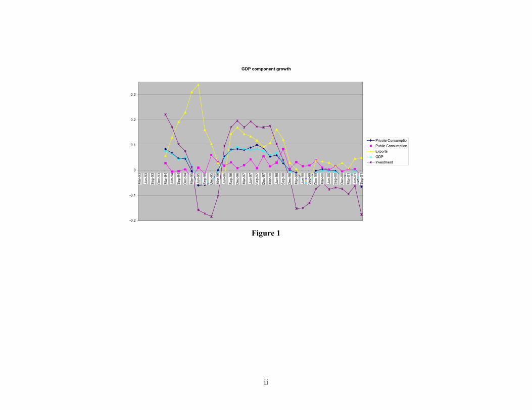
ii

GDP component growth

-0.2

-0.1

0

0.1

0.2

0.3

Mar

-93

Jun-

93

Sep-

93

Dec

-93

Mar

-94

Jun-

94

Sep-

94

Dec

-94

Mar

-95

Jun-

95

Sep-

95

Dec

-95

Mar

-96

Jun-

96

Sep-

96

Dec

-96

Mar

-97

Jun-

97

Sep-

97

Dec

-97

Mar

-98

Jun-

98

Sep-

98

Dec

-98

Mar

-99

Jun-

99

Sep-

99

Dec

-99

Mar

-00

Jun-

00

Sep-

00

Dec

-00

Mar

-01

Jun-

01

Sep-

01

Private ConsumptioPublic ConsumptionExportsGDPInvestment

Figure 1

iii

Export price and volumen growth

80.0

85.0

90.0

95.0

100.0

105.0

110.0

115.0

120.0

M-90

S-90

M-91

S-91

M-92

S-92

M-93

S-93

M-94

S-94

M-95

S-95

M-96

S-96

M-97

S-97

M-98

S-98

M-99

S-99

M-00

S-00

M-01

S-01

-0.2

-0.1

0

0.1

0.2

0.3

0.4

PriceQuantity

Figure 2

iv

Spreads Argentina

-600

-400

-200

0

200

400

600

12/2

9/19

95

3/29

/199

6

6/29

/199

6

9/29

/199

6

12/2

9/19

96

3/29

/199

7

6/29

/199

7

9/29

/199

7

12/2

9/19

97

3/29

/199

8

6/29

/199

8

9/29

/199

8

12/2

9/19

98

3/29

/199

9

6/29

/199

9

9/29

/199

9

12/2

9/19

99

3/29

/200

0

6/29

/200

0

9/29

/200

0

12/2

9/20

00

3/29

/200

1

6/29

/200

1

9/29

/200

1

12/2

9/20

01

Arg-EMBI+Arg-BrasArg-MéxArg-Ven15 per. Mov. Avg. (Arg-EMBI+)

Figure 3

v

Figure 4a

Public debt to GDP ratios

0.3

0.35

0.4

0.45

0.5

0.55

III-98 IV-98 I-99 II-99 III-99 IV-99 I-00 II-00 III-00 IV-00 I-01 II-01

Assumption GDP growth of 3 percent after II-98

ActualCounterfactual

vi

Figure 4b

Current account

-0.1

-0.09

-0.08

-0.07

-0.06

-0.05

-0.04

-0.03

-0.02

-0.01

0III-98 IV-98 I-99 II-99 III-99 IV-99 I-00 II-00 III-00 IV-00 I-01 II-01

Actual Counterfactual 4 per. Mov. Avg. (Actual )4 per. Mov. Avg. (Counterfactual )

vii

Figure 4c

Additional external debt as a share of GDP

-0.05

0

0.05

0.1

0.15

0.2

0.25

III-98 IV-98 I-99 II-99 III-99 IV-99 I-00 II-00 III-00 IV-00 I-01 II-01

viii

Table 2. Fiscal accounts

1993 1994 1995 1996 1997 1998 1999 2000 2001Current revenues 21.2 19.5 19.0 17.2 18.7 18.8 19.6 19.8 18.9

Social Security contributions 5.6 5.5 5.3 3.8 4.2 4.0 3.8 3.8 3.6Other 15.5 14.1 13.7 13.5 14.5 14.8 15.8 16.0 15.4

Primary spending 19.1 18.7 18.4 17.8 18.4 18.1 19.4 18.9 18.4Social security payments 5.3 5.9 6.1 5.7 5.9 5.8 6.1 6.1 6.2Other 13.8 12.8 12.4 12.1 12.5 12.3 13.2 12.8 12.3

Factor payments 1.2 1.2 1.6 1.7 2.0 2.2 2.9 3.4 3.6Primary surplus 2.2 0.8 0.6 -0.5 0.4 0.8 0.3 1.0 0.5Primary surplus excluding social security 1.8 1.3 1.3 1.4 2.1 2.7 2.6 3.3 3.1Factor payments 1.2 1.2 1.6 1.7 2.0 2.2 2.9 3.4 3.6Social security balance 0.4 -0.4 -0.7 -1.9 -1.7 -1.8 -2.3 -2.4 -2.6Overall balance 0.9 -0.4 -1.0 -2.2 -1.6 -1.4 -2.6 -2.4 -3.0Source: Ministerio de Economia

ix

Table 3. Accounting for changes in primary revenues and spendingTax revenue Primary spending

Levels Logs Levels Logs

GDP 0.19 1.47 0.09 0.72

(10.6) (10.7) (5.5) (5.5)

Dummy

post 2000.I 1000 0.11 185 0.015

(4.9) (4.7) (0.5) (0.7)

R2 0.84 0.84 0.54 0.53

N 31 31 31 31

Source: Own calculations based on data published by the Ministry of the Economy. T-stats in parenthesis

x

Fiscal balance and its components

-0.06

-0.04

-0.02

0

0.02

0.04

0.06

I-94

II - 9

4III

- 94

IV -

94

I - 9

5II

- 95

III -

95IV

-95

I-96

II-96

III-9

6IV

-96

I-97

II-97

III-9

7IV

-97

I-98

II-98

III-9

8IV

-98

I-99

II-99

III-9

9IV

-99

I-00

II-00

III-0

0

IV-0

0I-0

1II-

01III

-01

sprimxssint/pibSaldSS/pibFiscal balance

Figure 5

xi

Table 4Accounting for the increase in public debt

Debt as of 12/94 80.3

Debt as of 12/00 123.0

Total increase in gross debt 42.7

Increase in gross assets (collaterals and cash) 11.7

Increase in net debt 31.0

Cumulative deficit 1995-2000 21.8

- of which social security deficit 30.9

Capitalized interest and valuation changes -1.2

Recognized debt and other obligations 10.4

Memo: assets of the private pension funds 12/00 21.0

xii

Multilateral exchange rate and spread between Argentina and Mexico

-500

0

500

1000

1500

2000

2-Jan

-9817

-Feb-98

90

100

110

120

130

140

150

160

Spread Arg MexMultilateral XR

Figure 6

xiii

Y BP FC’

_ FC

IS Y

B A

Y’

I’ I I

Figure 7: Before and after the sudden stop

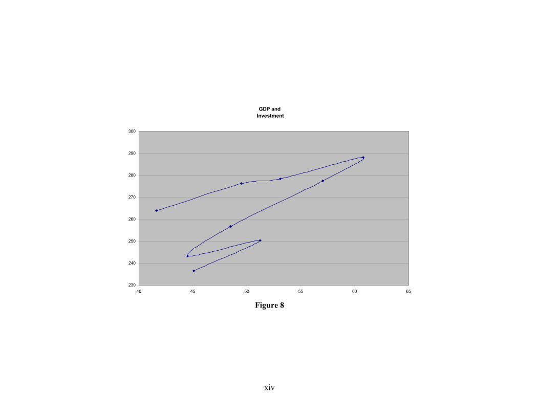
xiv

GDP and Investment

230

240

250

260

270

280

290

300

40 45 50 55 60 65

Figure 8

xv

Y BP FC

_ FC’

IS IS’

Y

Y ‘

I I’ I

Figure 9: Contractionary Fiscal Contraction

xvi

Y BP

_ A IS

B D IS’

FC

FC’

I

Figure 10: Fiscal contraction and self-fulfilling pessimism

xvii

Y BP

FC’

_ FC

IS’

IS

Y Y’

I’ I I

Figure 11: Contractionary Devaluation

xviii

Table 5 Debt-Service / Exports Ratios

Selected Countries(percent, 1999)

Country Total Debt Service/Exports Interest Payments/ExportsArgentina 72 30

Bolivia 37 12Brazil 106 24Chile 25 9China 9 3

Czech Republic 11 4Ecuador 26 13Estonia 13 4Hungary 27 5

India 16 6Indonesia 29 10

Korea 26 4Malaysia 5 2Mexico 28 8Pakistan 26 10Panama 8 5

Peru 32 20Poland 19 5Russia 12 5

South Africa 13 4Thailand 22 9

Source: Global Development Finance 2001, World Bank.

xix

Y BP FC’ FC

_ IS’

IS

Y’ A

Y

I I’ I

Figure 12: Devaluation plus pesification.

xx