INTERNATIONAL JOURNAL OF CLIMATOLOGY, VOL. 11,889-896 (1991) 551.524.3755 1.583.14(410.1)

THE ANNUAL PERIOD OF FREEZING TEMPERATURES IN CENTRAL ENGLAND: 1850-1989

CHRIS WATKINS Climatic Research Unit, School of Environmental Sciences, University of East Anglia. Norwich NR4 7TJ. UK*

Received 21 June 1990 Revised 7 March 1991

ABSTRACT The daily central England temperature (CET) series is examined for evidence of long-term changes in the duration of the annual freeze season by analysing the timing of the first and last days of winter that record a CET value of 0°C or lower. A statistically significant inverse relationship is found to exist between freeze season duration and time. A linear regression model demonstrates that the rate of decline is about 2 days per decade. This could be explained by a rise in air temperature. An overview of statistical theory is given and the model assumptions are tested.

KEY WORDS Central England temperature Freeze season Rising air temperature Policy

INTRODUCTION

In the past, many working practices in applying climatology to forward planning were based on an assumed constancy of climate (Lamb, 1982). Although this practice was common until recently it is widely felt to be unsatisfactory today. Many articles have appeared in the press and scientific literature in recent years that show that the common perception of climate is changing. Much but not all of the attention is focused on the possibility that man’s activities may have side-effects that disturb the climate regime. Causes and mechanisms of climatic change are discussed by Lamb (1988), global and hemispheric temperature variations between 1861 and 1984 have been analysed by Jones et al. (1986), and the impacts and policy implications of global warming are addressed by Warrick and Jones (1 988). The relationship, if any, between hemispheric temperature trends and freeze season duration changes, is of interest to agriculturalists, climate modellers, and policy analysts among others (Skaggs and Baker, 1985). In the case of policy making, past decisions concerning regional agriculture and industry may have been made without the behaviour of climate being considered at all.

The very mild winters of 1988, 1989 and 1990 in England (Hulme and Jones, 1991) could be the result of a random fluctuation in the climate. However, variations can be superimposed on a trend (Wright, 1976), and recent mild winters could be part of a long-term process of change. Better knowledge of the pace, direction and magnitude of climatic change is required.

A number of contemporary studies provide objective means of indicating the extent and intensity of such climatic changes. Annual and seasonal air temperatures at three stations in Greece were investigated by Giles and Flocas (1984) for non-random changes in persistence, trend and fluctuation. Skaggs and Baker (1985) considered the growing season in Minnesota in terms of both duration and the beginning and ending dates. Suckling (1986a) demonstrated the value of using specific event data (e.g. daily temperature thresholds) to identify climatic trends that may be undetectable when using monthly averages, and Suckling (1986b)

* Present address: Strategic Planning Section, Department of Planning and Property, Norfolk County Council, Norwich NRl 2DH, UK.

0899-841 8/91/080889-08%05.00 0 1991 by the Royal Meteorological Society

890 C. WATKINS

examined the fluctuating date of the last spring freeze in the south-eastem USA. The statistical properties of freeze date variables and the length of the growing season were discussed by Waylen and LeBoutillier (1989) and applied to sites in Saskatchewan and Florida. That paper also points to the many human activities that depend upon, or are affected by, some critical threshold level of the temperature variable, above or below which economic and or social costs are encountered.

THE DATA

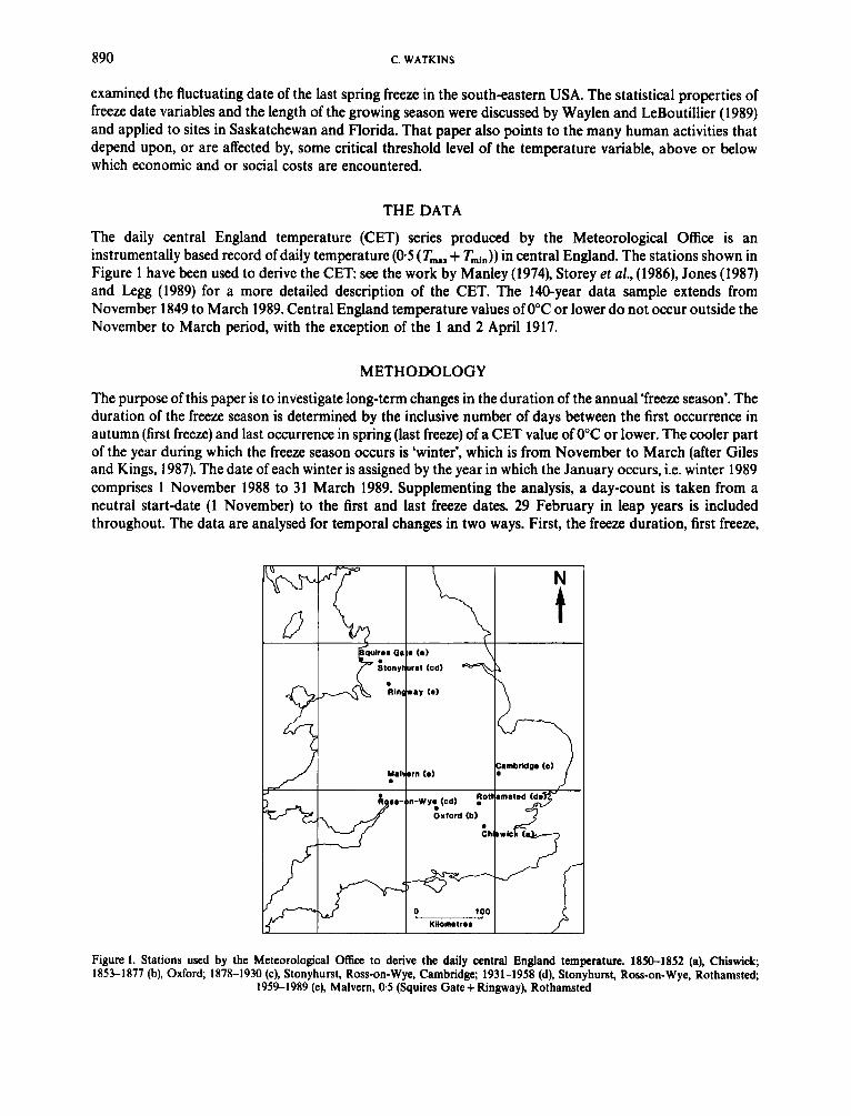
The daily central England temperature (CET) series produced by the Meteorological Office is an instrumentally based record of daily temperature (0-5 (T,,, + Tmin)) in central England. The stations shown in Figure 1 have been used to derive the CET see the work by Manley (1974), Storey et al., (1986), Jones (1987) and Legg (1989) for a more detailed description of the CET. The 140-year data sample extends from November 1849 to March 1989. Central England temperature values of 0°C or lower do not occur outside the November to March period, with the exception of the 1 and 2 April 1917.

METHODOLOGY

The purpose of this paper is to investigate long-term changes in the duration of the annual ‘freeze season’. The duration of the freeze season is determined by the inclusive number of days between the first occurrence in autumn (first freeze) and last occurrence in spring (last freeze) of a CET value of 0°C or lower. The cooler part of the year during which the freeze season occurs is ‘winter’, which is from November to March (after Giles and Kings, 1987). The date of each winter is assigned by the year in which the January occurs, i.e. winter 1989 comprises 1 November 1988 to 31 March 1989. Supplementing the analysis, a day-count is taken from a neutral start-date (1 November) to the first and last freeze dates. 29 February in leap years is included throughout. The data are analysed for temporal changes in two ways. First, the freeze duration, first freeze,

N

t

Figure 1. Stations used by the Meteorological Office to derive the daily central England temperature. 1850-1852 (a), Chiswick; 1853-1877 (b), Oxford; 1878-1930 (c), Stonyhurst, Ross-on-Wye, Cambridge; 1931-1958 (d), Stonyhurst, Ross-on-Wye, Rothamsted;

1959-1989 (e), Malvern, 0.5 (Squires Gate+ Ringway), Rothamsted

FREEZING TEMPERATURES IN CENTRAL ENGLAND 89 1

and last freeze unsmoothed values are regressed on time. Second, the record is divided into two parts, the means of which are compared in a t test.

STATISTICAL THEORY

Many studies of freeze variables assume that the data are normally distributed (Thom and Shaw (1958)). Any deviations from normality may be considered in terms of estimates of the higher moments of distributions. In particular, the coefficients of skewness and kurtosis are useful in assessing the degree of fit of the observed data to theoretical distributions. They are, however, considered to be unstable at small sample sizes (Waylen and LeBoutillier, 1989). The moment coefficient of skewness, rl, is

and the moment coefficient of kurtosis, r,, is

In equations (1) and (2), observation xi, 1, 2 , . . . , ", has mean p and standard deviation a. If the population from which the sample is drawn is normal, skewness and kurtosis should be near 0 and 3, respectively.

Correlation

Pearson's product-moment correlation coefficient (r) is a measure of the degree of linear relationship between two random variables. Theoretically defined as the ratio of the covariance of X and Y to the product of the variances of X and Y, the equation for r may be written

where ( X i , K) is a set of n bivariate sample observations.

hypothesis of statistical independence between the two variables, i.e. that r is really equal to zero. Assuming that X and Y have a bivariate normal distribution, the t distribution can be used to test the null

Regression

The main tool of analysis used in this paper is regression. The method is firmly established but its assumptions are sometimes neglected. When n pairs of observations (Xl, Yl), ( X 2 , Y2), . . . , (X, , , Y,,) are considered the relationship between the independent (X) and dependent (Y) variables can be written as

(4) for i = 1,2, . . . , n, so that the sum of squares of deviations from the true line is minimized.

The form of the model in equation (4) permits the use of inferential statements about the regression coefficients. An implicit assumption of the model is that the error term, q, is normally distributed, homoscedastic and independent (Hays and Winkler, 1971; Gregory, 1978; Draper and Smith, 1981). It is standard to investigate the residuals as a check on the efficacy of the linear regression procedure.

Yr =Bo + B1 Xi + Ei

Test of residuals

and is calculated as follows The chi-square test may be used to measure goodness of fit between observed and thzoretical distributions

as

X2' 2 (+Ei)2/Ei i = 1

(5)

892 C. WATKINS

where 0, and E , are the observed and expected frequencies (see Caswell, 1989). In this case the residuals are compared with a normal distribution.

The problem of serial correlation frequently arises in time-series analysis when fitting a linear model. The Durbin-Watson statistic (see Durbin and Watson, 1950,1951) tests the null hypothesis of independence in the error term against the alternative of the first-order autoregressive model. The statistic, d, is defined by

Upper and lower bounds to the critical values, d , and dL, exist for pre-specified levels of significance. For a discussion on the accuracy of the d, approximation see Durbin and Watson (1971). For tests of independence against negative serial correlation, the procedure is repeated as above, but (4 - d) is considered in place of d.

The statistical tests that use the t distribution in this paper are carried out at the 0.01 significance level. F , x2 and d tests use the 0.05 level to decrease the probability of committing Type I1 errors.

ANALYSIS

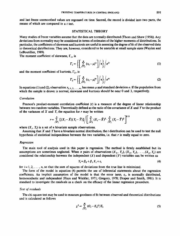
The interannual variations in freeze season duration are shown in Figure 2, and the least-squares regression line is fitted to the original data.

Descriptiue statistics

The sample descriptive statistics are specified in Table I. The skew coefficients in Table I(a) show that the distributions of the dates of first and last freeze are somewhat asymmetric. The positive skew in first freeze results from a few very late dates. Conversely, the last freeze distribution contains a few very early freezes. The duration coefficient indicates a slight negative skew, which is consistent with the tendency towards occasionally later first freezes and earlier last freezes.

1 25

100 A u)

P s g 75

5 P

0 50

25

0 1860 1880 ls00 1 920 1940 1980 1980

llme

Inter-annual Variations In the Freeze Season Duration: 1850 to 1 Wg

with fitted line of least squares

Figure 2. Interannual variations in the freeze season duration: 1850-1989, with fitted line of least-squares

FREEZING TEMPERATURES IN CENTRAL ENGLAND 893

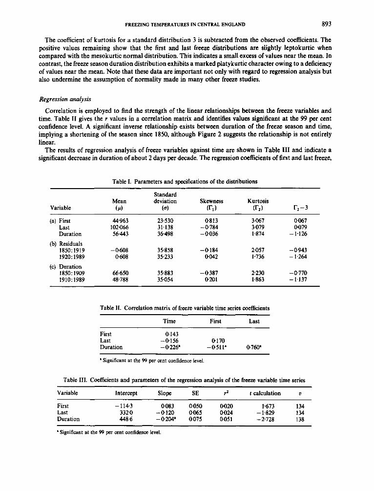
The coefficient of kurtosis for a standard distribution 3 is subtracted from the observed coefficients. The positive values remaining show that the first and last freeze distributions are slightly leptokurtic when compared with the mesokurtic normal distribution. This indicates a small excess of values near the mean. In contrast, the freeze season duration distribution exhibits a marked platykurtic character owing to a deficiency of values near the mean. Note that these data are important not only with regard to regression analysis but also undermine the assumption of normality made in many other freeze studies.

Regression analysis

Correlation is employed to find the strength of the linear relationships between the freeze variables and time. Table I1 gives the r values in a correlation matrix and identifies values significant at the 99 per cent confidence level. A significant inverse relationship exists between duration of the freeze season and time, implying a shortening of the season since 1850, although Figure 2 suggests the relationship is not entirely linear.

The results of regression analysis of freeze variables against time are shown in Table 111 and indicate a significant decrease in duration of about 2 days per decade. The regression coefficients of first and last freeze,

Table I. Parameters and specifications of the distributions

Mean deviation Skewness Kurtosis Standard

Variable ( A (4 (I-,) (I-, ) I-,-3

(a) First 44.963 23.530 0813 3.067 0067 Last 102.066 31.138 -0784 3.079 0079 Duration 56443 36.498 -0.036 1.874 - 1.126

(b) Residuals 1850: 1919 -0.608 35.858 -0.184 2-057 - 0.943 1920: 1989 0608 35.233 0.042 1.736 - 1.264

1850: 1909 66.650 35883 -0.387 2.230 - 0.770 1910: 1989 48.788 35-054 0 2 0 1 1463 - 1.137

(c) Duration

Table 11. Correlation matrix of freeze variable time series coefficients

Time First Last

First 0.143 Last -0.156 0.170 Duration - 0.226' -0.511' 0760'

a Significant at the 99 per Cent confidence level.

Table 111. Coefficients and parameters of the regression analysis of the freeze variable time series

Variable Intercept Slope SE r2 t calculation U

First - 114.3 0.083 0.050 0020 1.673 134 Last 332.0 -0120 0.065 0024 - 1.829 134 Duration 448.6 - 0204' 0.075 0.05 1 - 2.728 138

' Significant at the 99 per cent confidence level.

894 C. WATKINS

75

60 -

45 -

30-+

15 - - !!

a 1 0

-15

-30 -

-45 -

-60 -

-75

although not significant, show that of this amount, some 0.8 days are attributable to the later occurrence of first freeze and 1.2 days to the earlier occurrence of last freeze.

+ + + + + + +

+ + *+ + + ++++++ + U + + + + ++ +++ +I++ + + +

+ ++++ + #

+ + + + + ++ + +++ ++ +

* + ' + + + + + f + +

+ + + + + + + * ++++I+

+U

+ *+ + + ' ++ "

+ + ++ + + + + + + + ++ +

:-#+ + +

+ t + ++ + + + +

+ + + t + + + +

I I I I I I 1850 1870 1890 1910 1930 1950 1970 l!

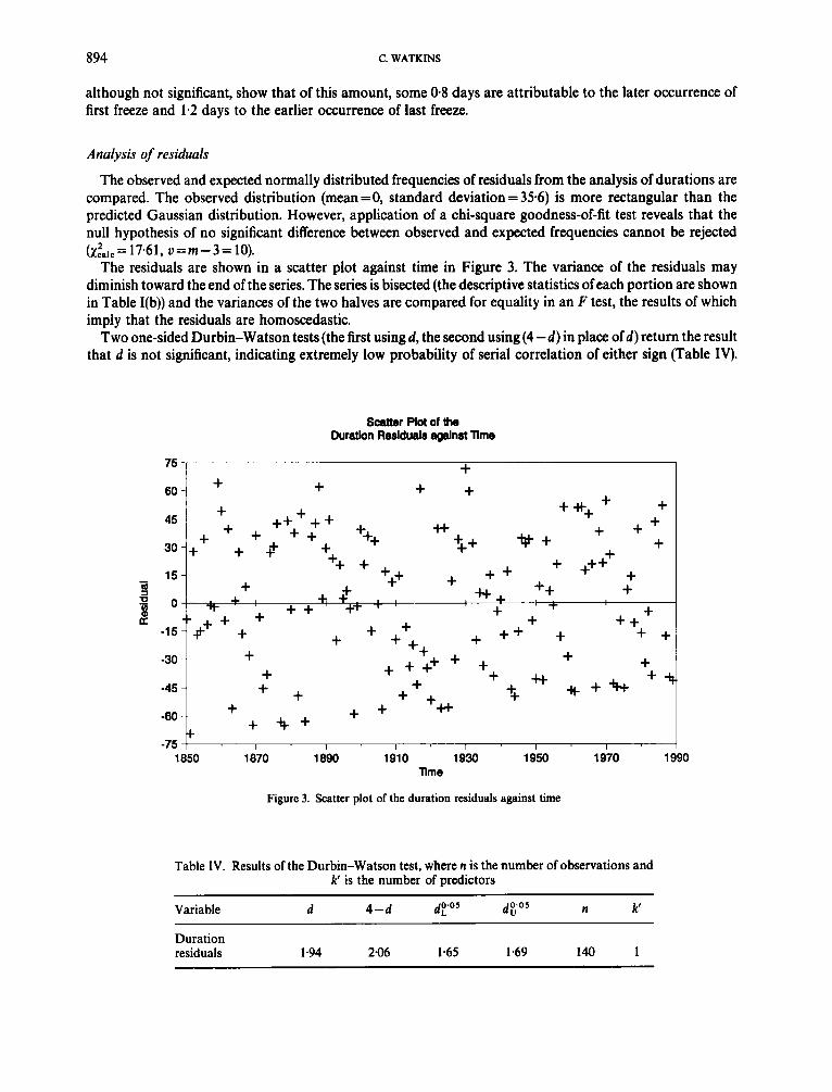
Analysis of residuals

The observed and expected normally distributed frequencies of residuals from the analysis of durations are compared. The observed distribution (mean =0, standard deviation = 35.6) is more rectangular than the predicted Gaussian distribution. However, application of a chi-square goodness-of-fit test reveals that the null hypothesis of no significant difference between observed and expected frequencies cannot be rejected (xZalc= 17.61, o=m-3= 10).

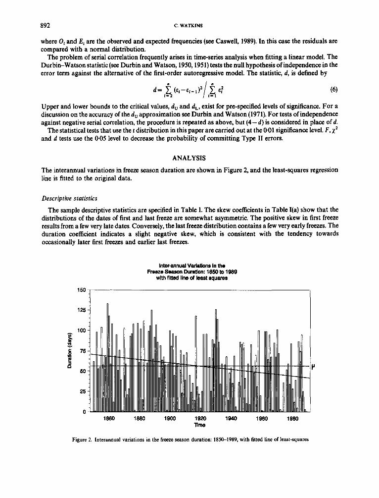
The residuals are shown in a scatter plot against time in Figure 3. The variance of the residuals may diminish toward the end of the series. The series is bisected (the descriptive statistics of each portion are shown in Table I(b)) and the variances of the two halves are compared for equality in an F test, the results of which imply that the residuals are homoscedastic.

Two one-sided Durbin-Watson tests (the first using d, the second using (4 -d) in place of d) return the result that d is not significant, indicating extremely low probability of serial correlation of either sign (Table IV).

Figure 3. Scatter plot of the duration residuals against time

90

Table IV. Results of the Durbin-Watson test, where n is the number of observations and k' is the number of predictors

Variable d 4-d dFo5 d E o 5 n k'

Duration residuals 1.94 2.06 1.65 1.69 140 1

FREEZING TEMPERATURES IN CENTRAL ENGLAND 895

Total Freeze Season days per Decade: Departure from Long-term Average

wlth fined line of least squares

200 I

50 St longer freeze seasons n 100

2 50 s g o t:

-50

-100

-1 50

-200

shorter freeze seasons

1860's 1880's 1900's 1920's 194v.s 1960's 1980's llme

Figure 4. Total freeze season days per decade: departure from long-term average, with fitted line of least-squares

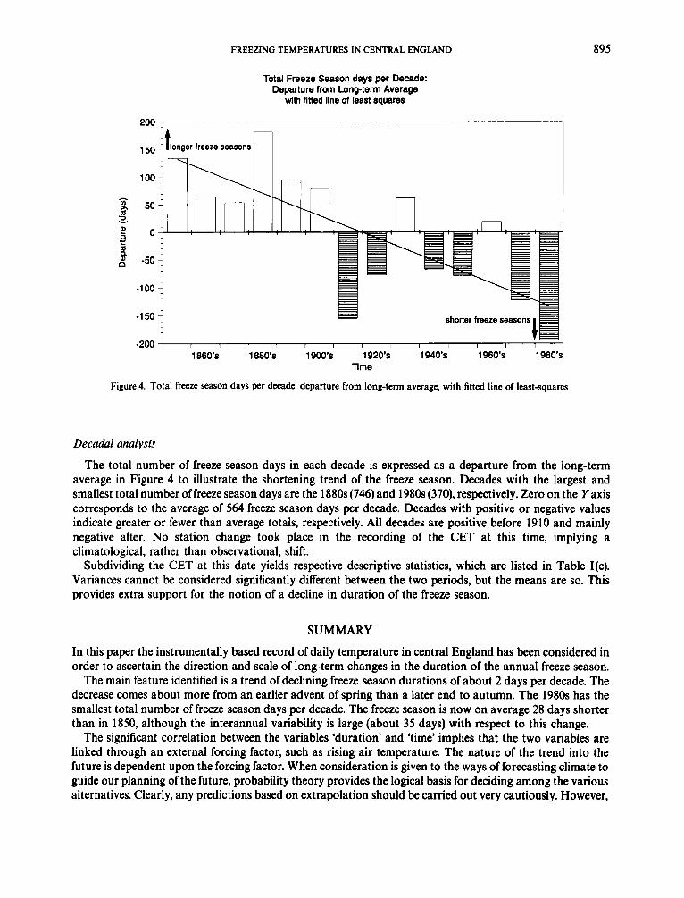
Decadal analysis

The total number of freeze season days in each decade is expressed as a departure from the long-term average in Figure 4 to illustrate the shortening trend of the freeze season. Decades with the largest and smallest total number of freeze season days are the 1880s (746) and 1980s (370), respectively. Zero on the Y axis corresponds to the average of 564 freeze season days per decade. Decades with positive or negative values indicate greater or fewer than average totals, respectively. All decades are positive before 1910 and mainly negative after. No station change took place in the recording of the CET at this time, implying a climatological, rather than observational, shift.

Subdividing the CET at this date yields respective descriptive statistics, which are listed in Table I(c). Variances cannot be considered significantly different between the two periods, but the means are so. This provides extra support for the notion of a decline in duration of the freeze season.

SUMMARY

In this paper the instrumentally based record of daily temperature in central England has been considered in order to ascertain the direction and scale of long-term changes in the duration of the annual freeze season.

The main feature identified is a trend of declining freeze season durations of about 2 days per decade. The decrease comes about more from an earlier advent of spring than a later end to autumn. The 1980s has the smallest total number of freeze season days per decade. The freeze season is now on average 28 days shorter than in 1850, although the interannual variability is large (about 35 days) with respect to this change.

The significant correlation between the variables 'duration' and 'time' implies that the two variables are linked through an external forcing factor, such as rising air temperature. The nature of the trend into the future is dependent upon the forcing factor. When consideration is given to the ways of forecasting climate to guide our planning of the future, probability theory provides the logical basis for deciding among the various alternatives. Clearly, any predictions based on extrapolation should be carried out very cautiously. However,

896 C. WATKINS

although usually poor, forecasts obtained in this way are still sometimes of value to agriculture and other managerial services.

If the freeze season is shortening it should follow that the reciprocal more temperate part of the year (growing season) is lengthening a corresponding amount. Should this be the case it may be potentially useful with regard to crop types, water management, and energy consumption. There may be some scope therefore to allow somewhat wider margins in the planning process for the potential impacts of climatic change.

ACKNOWLEDGEMENTS

I am grateful to C. K. Folland, Meteorological Office, for supplying the daily central England temperature series and Phil Jones, Climatic Research Unit, for useful advice throughout this work. Thanks are also due to a referee for useful recommendations, and to Tom Wigley, Climatic Research Unit, for the original discussion.

REFERENCES

Caswell, F. 1989. Success in Statistics, 2nd edn, Murray, London, p. 356. Draper, N. R. and Smith, H. 1981. Applied Regression Analysis, 2nd edn, Wiley, New York, p. 709. Durbin, J. and Watson, G. S. 1950. ‘Testing for serial correlation in least squares regression. I’, Biometrika, 37, 409-428. Durbin, J. and Watson, G. S. 1951. ‘Testing for serial correlation in least squares regression. 11’, Biometrika, 38, 159-178. Durbin, J. and Watson, G. S. 1971. ‘Testing for serial correlation in least squares regression. 111’, Biometrika, !i8, 1-19. Giles, B. D. and Flocas, A. A. 1984. ‘Air temperature variations in Greece. Part I. Persistence, trend, and fluctuations’, J. Climatol., 4,

Giles, B. D. and Kings, J. 1987. ‘Good King Wenceslas: alternative strategies for the U.K. Department of Health and Social Security

Gregory, S. 1978. Statistical Methods and the Geographer, 4th edn, Longman, New York, p. 240. Hays, W. L. and Winkler, R. L. 1971. Statistics: Probability, Infmence, and Decision, Holt, Rinehart and Winston, New York, p. 937. Hulme, M. and Jones, P. D. 1991. ‘Temperatures and windiness over the United Kingdom during the winters of 1988/89 and 1989/90

Jones, D. E. 1987. ‘Daily Central England Temperature: recently constructed series’, Weather, 42, 130-133. Jones, P. D., Wigley, T. M. L. and Wright, P. B. 1986. ‘Global temperature variations between 1861 and 1984, Nature. 322,430-434. Lamb, H. H. 1982. Climate, History, and the Modern World, Methuen, London, p. 387. Lamb, H. H. 1988. Weather, Climate and Human Affairs. A Book of Essays and Other Papers, Routledge, London, p. 364. Leg& T. P. 1989. ‘Removal of urbanization effects from the Central England temperature data sets’, Long-rangeforecasting and Climate

Manley, G. 1974. ‘Central England Temperatures: monthly means 1659-1973’, Q. J. R. Meteorol. Soc., 100, 389-405. Skaggs, R. H. and Baker, D. G. 1985. ‘Fluctuations in the length of the growing season in Minnesota’, Climatic Change, 7,403-414. Storey, A., Folland, C. K. and Parker, D. E. 1986. ‘A homogeneous archive ofdaily Central England Temperature 1773 to 1985 and new

monthly averages 1974 to 1985’, Synoptic Climatology Branch Memorandum No. 107, U.K. Meteorological Office, Bracknell. Suckling, P. W. 1986a. ‘Climatic change in Georgia as illustrated by the frequency of freezing and hot days’, Southeastern Geogr., 26,

25-35. Suckling, P. W. 1986b. ‘Fluctuations of last spring-freeze dates in the southeastern United States’, Phys. Geogr., 7, 239-245. Thom, H. C. S. and Shaw, R. H. 1958 ‘Climatological analysis of freeze data for Iowa’, Mon. Wea. Reu., 86, 251-257. Warrick, R. A. and Jones, P. D. 1988. ‘The greenhouse effect, impacts and policy implications’, Forumfor Applied Research and Public

Waylen, P. R. and LeBoutillier, D. W. 1989. ‘The statistical properties of freeze date variables and the length of the growing season’,

Wright, P. B. 1976. ‘Recent climatic change’, in Chandler, T. J. and Gregory, S. (eds) The Climate ofthe British Isles, Longman, London,

531-539.

(DHSS)’, J . Climatol., 7, 129-143.

compared with previous years’, Weather, in press.

Memorandum No. 33, UK Meteorological Office, Bracknell.

Policy, Fall, 1988, Tennessee Valley Authority, pp. 48-62.

J . Climate, 2, 1314-1328.

pp. 224-247.