The 2016 Antarctic Ozone Hole Summary: Report #7, Sunday 25 September 2016

Paul Krummel and Paul Fraser CSIRO Oceans and Atmosphere Aspendale, Victoria

Summary

For the 2016 ozone hole we will again be reporting images and metrics calculated from both the OMI and OMPS data products (see the instrumentation section for a description of these). Please note that due to operational reasons, the OMPS Level 3 global gridded daily total ozone column products provided by NASA run 4-5 days behind the current day.

August

In late-July there were some excursions below 220 DU (down to 170-180 DU; record lows) around the edge of the polar night, which resulted in an ozone hole area of approximately 2 million km2. However, these recovered during the first week of August. The second week of August saw the 2016 ozone hole start to form in earnest, with the ozone hole area peaking at almost 7 million km2 on 12 August, and the ozone minima dropping to 184 DU on 8 August. The third week of August showed only minimal growth in the Antarctic ozone hole, with the area metric reaching 4.2 million km2 and minima dropping to 177 DU by 18 August. Of

note is that the forecast 45-75S heat flux and 60-90S zonal mean temperatures at 50 & 100 hPa indicate a rapid change in the next 10 days, with a larger amount of heat transported towards the pole and corresponding jump in the temperature (to the highest 10th percentile). The fourth week of August saw the ozone hole area double in size to be at 8.6 million km2 by 26 August, while the ozone hole minima dropped to 166 DU. However, the total column ozone images indicate some strong wave activity during 20-26 August with the ozone hole/polar vortex becoming quite elongated, and has resulted in the Australian Antarctic

bases being under a high ridge of ozone during 23-26 August. The 45-75S heat flux and 60-90S zonal mean temperatures at 50 & 100 hPa also suggest some sort of meteorological disturbance with larger amounts of heat being transported towards the pole (a more negative heat flux) and corresponding warmer stratospheric temperatures (in the highest 10th percentile range). The forecast data are suggesting further rapid changes in both the heat flux and temperatures over the next ten days which could have considerable impact on the growth of the 2016 ozone hole. The last 5 days of August and beginning of September saw a continued

distortion in the ozone hole with the elongation rotating from being along an axis of 0 – 180 longitude on

26 August to being along an axis of 105E – 75W longitude by 2 September. During this period the ozone hole continued to form, with it almost completely enclosed by 2 September, and a large pocket of low ozone present immediately south of South America on 2 September.

September

By 2 September the ozone hole area was at 15.1 million km2 and the minima had dropped to a record breaking 113 DU – however, this minima should be treated with some caution as it was found to be one pixel that occurred next to one of the thin missing data stripes, and it will be interesting to see if the OMPS instrument has seen this low minima when the data become available. The ozone hole area reached a high of 19.1 million km2 on the 8th before dropping back to 16.4 million km2 on the 9th of September due to the large distortion in the ozone hole. The OMI minima data dropped further to a record breaking low of 104 DU on 3 September before increasing again to be at 162 DU by 9 September, close to the long-term 1979-2015 mean. The OMPS data dropped sharply to a minima on 3 September of 131 DU, however this is substantially higher than the OMI minima. The ozone hole underwent a quite severe distortion from 7 through to 9 September. The

distortion on 9 September was along an axis 45E – 105W longitude, with parts of the ozone hole reaching

approximately 55S latitude. During this time the 3 Australian Antarctic mainland bases (Mawson, Davis & Casey) where outside of the ozone hole, with a strong ridge of high ozone present to the south of Australia.

The 60-90S zonal mean temperatures at both 50 & 100 hPa continued to increase during the first 9 days of September, with both reaching levels on 9 September that are the warmest on record for this time of year (in the 1979-2015 timeframe). The forecast data are indicating that the temperatures will decrease again and stabilise over the next 10 days, perhaps indicating more stable polar vortex conditions. The distortion in the ozone hole continued on 10-11 September, however by 13 September the ozone hole had become symmetrical again. It remained this way for several days, but by 17 September was showing signs of distortion

again. The symmetry corresponded to drops in the 60-90S zonal mean temperatures at both 50 & 100 hPa suggesting more stable conditions. During this period the ozone hole area increased to just over 20 million km2 on 13 September before dropping back to about 19.5 million km2 by 17 September. The ozone minima dropped to 142 DU by 17 September, having first dipped down to 135 DU on the 13th of September. A repeating pattern of a period of distortion of the ozone hole followed by a period of more symmetrical behaviour is emerging, suggesting some strong wave activity around the polar vortex. The period 18-21 September was characterised by a more stable/symmetrical ozone hole which became distorted again during 22-23 September. This pattern of symmetry and distortions has resulted in the three Australian Antarctic mainland bases oscillating from being within the ozone hole to being under the ridge of high ozone. The ozone hole continued to grow during the third week of September reaching 22.6 million km2 on 22 September with the daily ozone deficit reaching 24.6 million tonnes on 21 September. The ozone minima continued to drop during the third week of September reaching 131 DU by the 23rd.

The 2016 ozone hole

Ozone hole area

In late-July there were some excursions below 220 DU around the edge of the polar night, which resulted in an ozone hole area of approximately 2 million km2. These essentially recovered during the first week of August, but by the second week of August the ozone hole appears to have started forming in earnest, peaking at almost 7 million km2 on 12 August before dropping back to 2.8 million km2 on 13 August. The third week of August saw only a small amount of growth in the ozone hole area, ending at 4.2 million km2 by 18 August. The fourth week of August saw the ozone hole area double in size, from approximately 4 million km2 on 19 August to 8.6 million km2 by 26 August. The ozone hole area increased rapidly during the last 5 days of August and beginning of September, to be at 15.1 million km2 by 2 September.

During the first week of September the ozone hole area reached a high of 19.1 million km2 on the 8th before dropping back to 16.4 million km2 on the 9th of September due to the large distortion in the ozone hole. From the 10th until the 17th of September the ozone hole area increased to just over 20 million km2 before dropping back to about 19.5 million km2 by 17 September. The ozone hole continued to grow during the third week of September reaching 22.6 million km2 on 22 September before dropping back slightly to 21.3 million km2 on 23 September.

Ozone deficit

The bottom panel of Figure 1 shows that by mid-August there were small levels of estimated daily ozone deficit corresponding to the above mentioned ozone hole areas. The estimated daily ozone deficit reached 1.9 million tonnes on 12 August before dropping back to < 0.5 million tonnes on 13 August. Similar to the ozone hole area, the daily ozone deficit grew slightly during the third week of August to be at 1.3 million tonnes on 18 August. During the fourth week of August the daily ozone deficit increased steadily to be at 4 million tonnes on 26 August. The last 5 days of August and beginning of September saw the daily ozone deficit start to increase more rapidly, to be at 6.8 million tonnes by 2 September.

By 9 September, the daily ozone deficit had only reached modest levels of around 8 million tonnes, which is well below the 1979-2015 average for this time of year and is similar to the levels seen in 2012 (which was one of the smallest ozone holes since the late 1980s). The period from the 10th to 17th September saw the daily ozone deficit continue to rise, reaching 16.7 million tonnes by the 17th. During the third week of September the daily ozone deficit continued to rise sharply, reaching 24.6 million tonnes on 21 September, before dropping back to 23.6 million tonnes by 23 September.

Ozone hole minima

In late-July there were some large excursions below 220 DU for several days that occurred right at the edge of the polar night, which should be treated with some caution as there is often large variability in this metric

during late July and the first few weeks of August. The ozone minima in late-July, as seen by both the OMI and OMPS instruments, dropped to between 170-180 DU, which are the lowest levels on record for this time of year. These levels recovered to be above 220 DU for most of the first week of August before the ozone minima once again dropped below 220 DU on 6 August and has remained below 220 DU since, dropping to 182 DU on 8 August and ending at 194 DU on 13 August. The variability in this metric is expected to reduce in the next two to three weeks as the polar night reduces and the ozone hole fully forms. The variability in this metric continued during the third and fourth weeks of August superimposed on an overall declining trend, with the ozone minima being at 177 DU on 18 August and 166 DU by 26 August. On 2 September the ozone hole minima (as seen by OMI) dropped sharply to 113 DU, which is the lowest on record for this time of year. This low value should be treated with caution, as on further investigation it was found to be one pixel that occurred next to one of the thin missing data stripes in the pocket of low ozone near South America (see Figure 3). It will be interesting to see if the OMPS data show this very low minima when data become available.

The OMI minima data dropped further to a record breaking low of 104 DU on 3 September before increasing again to be at 162 DU by 9 September, close to the long-term 1979-2015 mean. The OMPS data also dropped sharply to a minima on 3 September of 131 DU, however this is substantially higher than the OMI minima. By the 17th of September the ozone minima had dropped to 142 DU, having first dipped down to 135 DU on the 13th of September. The ozone minima continued to drop during the third week of September reaching 131 DU by the 23rd.

Average ozone in the hole

The average ozone amount in the hole (averaged column ozone amount in the hole weighted by area; Figure 2 bottom panel) shows a similar pattern to that of the ozone hole minima. The late-July average ozone amount reached 197 DU on 28 July (record low for that time of year), before recovering and then dropping below 220 DU again on 6 August, and ending at 212 DU on 13 August. The third week of August saw the average ozone amount in the hole stay at around 212-213 DU before dropping to 206 DU on 18 August. The following week saw the average ozone amount in the hole increase again before dropping to 198 DU by 26 August. During the last 5 days of August and beginning of September the average ozone amount in the hole continued to fluctuate between 200-206 DU, with the value dropping to 199 DU on 2 September.

By the 9th of September the average ozone amount in the hole had only dropped to 198 DU, which is higher than the long-term 1979-2015 mean and is similar to the 2012 ozone hole. The average ozone amount in the hole dropped rapidly during 10-17 September to be at 180 DU by the 17th. By the 23rd of September the average ozone amount in the hole had dropped to 168 DU.

Total column ozone images

The most recent 16 days of total column ozone ‘images’ over Australia and Antarctica from OMI are shown in Figure 3 and from OMPS are shown in Figure 4.

The late-July excursions below 220 DU can be clearly seen along the edge of the Antarctic polar night, before recovering during the first week of August. From 6 August onwards, the ozone hole can be seen forming again in several areas around the polar night. By the end of the second week of August the Antarctic polar night still covered most of Antarctica. What is in contrast to the 2015 Antarctic ozone hole, is that the strong

ridge of high ozone in the band immediately south of Australia between about 40-60S is present again in 2016, although it appears to be a bit patchy, possibly indicating some wave activity. During the third week of August the ozone hole can still be seen forming in several areas around the polar night. The next 2-3 weeks should see the 2016 ozone hole fully form as the polar night reduces. The polar vortex appears to have become quite distorted from 20 to 26 August most likely due to some strong wave activity, with the image

from 26 August showing an elongated ozone hole/polar vortex along an axis of 0 – 180 longitude. This resulted in the three Australian Antarctic mainland bases (Mawson, Davis & Casey) being under a strong ridge of high ozone during 23-26 August. The distortion of the ozone hole continued during 27 August to 2

September, with the elongation rotating from being along an axis of 0 – 180 longitude on 26 August to

being along an axis of 105E – 75W longitude by 2 September. During this period the ozone hole continued to form, with it almost completely enclosed by 2 September, and a large pocket of low ozone present immediately south of South America on 2 September.

The distortion on the ozone hole continued on 3 & 4 September, then on 5 & 6 September the ozone hole became somewhat more symmetrical, before undergoing quite a severe distortion from 7 through to 9

September. The distortion on 9 September was along an axis 45E – 105W longitude, with parts of the ozone

hole reaching approximately 55S latitude. During this time the 3 Australian Antarctic mainland bases (Mawson, Davis & Casey) where outside of the ozone hole, with a strong ridge of high ozone present to the south of Australia. The above mentioned distortion continued on 10-11 September, however by 13 September the ozone hole had become symmetrical again. It remained this way for several days, but by 17 September was showing signs of distortion again. A repeating pattern of a period of distortion of the ozone hole followed by a period of more symmetrical behaviour is emerging, suggesting some strong wave activity around the polar vortex. The period 18-21 September was characterised by a more stable/symmetrical ozone hole which became distorted again during 22-23 September. This pattern of symmetry and distortions has resulted in the three Australian Antarctic mainland bases oscillating from being within the ozone hole to being under the ridge of high ozone.

NASA MERRA heat flux and temperature

The MERRA 45-day mean 45-75S heat fluxes at 50 & 100 hPa are shown in Figure 5. A less negative heat flux usually results in a colder polar vortex, while a more negative heat flux indicates heat transported towards the pole (via some meteorological disturbance/wave) and results in a warming of the polar vortex. The

corresponding 60-90S zonal mean temperatures at 50 & 100 hPa are shown in Figure 6, these usually show an anti-correlation to the heat flux.

At 50 hPa, the type 1 PSC (HNO3.3H2O) formation threshold temperature (195 K) was reached in late June. At 100 hPa, the threshold temperature was reached during the second week of July.

May, June, July

During mid-May to mid-June the 45-75S heat flux at 50 & 100 hPa was at near record low levels compared to the 1979-2015 range, indicating larger amounts of heat transported towards the pole. Correspondingly,

the 60-90S zonal mean temperatures at 50 & 100 hPa were higher than average being in the 70-90th

percentile of the 1979-2015 range. From mid-June to mid-July, the 45-75S heat flux at 50 hPa gradually

returned to be at the mean of the 1979-2015 range, where it remained until the end of July. The 45-75S heat flux at 100 hPa during the same period rose to be at the 30th percentile mark of the 1979-2015 range,

where it remained until the end of July. The 60-90S zonal mean temperatures at 50 & 100 hPa from mid-June to mid-July dropped from the 70-90th percentile down to the lower 10-30th percentile range. This was

relatively short lived and by the end of July the 60-90S temperatures at both 50 & 100 hPa levels had both spiked to be close to the upper 90th percentile mark.

August

The first two weeks of August saw the 45-75S heat flux at 50 & 100 hPa drop to, or remain at, approximately

the 30th percentile mark of the 1979-2015 range. The corresponding 60-90S zonal mean temperatures at 50 & 100 hPa during the first two weeks of August dropped to the lower 30-50 percentile of the 1979-2015

range, indicating a colder than average low-mid stratosphere. The third week of August saw the 45-75S heat flux at 50 & 100 hPa remain at approximately the 30th percentile mark of the 1979-2015 range. However, the forecast data (shown in orange) at both the 50 & 100 hPa levels indicates a rapid drop in the heat flux over the next 10 days, suggesting a larger amount of heat transported towards the pole. Correspondingly, the 60-

90S zonal mean temperatures at 50 & 100 hPa during the third week of August remained in the lower 30-50 percentile of the 1979-2015 range, with the forecast data indicating a rapid rise in the temperatures during the next 10 days to be at or above the highest 10th percentile mark of the 1979-2015 range by end of August.

During the fourth week of August the 45-75S heat flux at 50 & 100 hPa dropped to be in the lower 30th-10th percentile range of the 1979-2015 average, with the forecast data suggesting further rapid drops in this variable over the next 10 days. This is consistent with some strong wave activity allowing transport of heat towards the pole. Correspondingly, the stratospheric temperatures have risen rapidly with the 50 hPa 60-

90S zonal mean temperature reaching the 90th percentile mark of the 1979-2015 range by 26 August, while at 100 hPa it reached well into the highest 10th percentile of the 1979-2015 range. The forecast data for the

next 10 days suggests further rapid rises in the temperatures at these two levels. The 45-75S heat flux at 50

& 100 hPa dropped to be in the lowest 10th percentile range of the 1979-2015 average during the last 5 days of August and beginning of September, with the forecast data suggesting further rapid drops in this variable over the next 10 days. During the same period, the stratospheric temperatures have continued to rise with

the 50 hPa 60-90S zonal mean temperature tracking along the 90th percentile mark of the 1979-2015 range, while at 100 hPa it continued to be in the highest 10th percentile of the 1979-2015 range. The forecast data for the next 10 days suggests further rapid rises in the temperatures at these two levels.

September

The drop in the 45-75S heat flux at 50 & 100 hPa continued during the first week of September with value reached on 9 September being the lowest recorded in the 1979-2015 timeframe for this time of year. The forecast data are suggesting that the heat flux may stabilise or increase again over the next 10 days. The

corresponding 60-90S zonal mean temperatures at both 50 & 100 hPa continued to increase during this period with both reaching levels that are the warmest on record (in the 1979-2015 timeframe) for this time of year on 9 September. The forecast data are indicating that the temperatures will decrease again and stabilise over the next 10 days, perhaps indicating more stable polar vortex conditions. As predicted, the 45-

75S heat flux at both 50 & 100 hPa levels increased over the 10-16 September timeframe, but this may be temporary with the forecast data at the 100 hPa level showing further decreases in this metric (more heat transported towards the pole) while at the 50 hPa level the forecast data suggest a plateau over the next 10

days. As expected, the 60-90S zonal mean temperatures dropped again during 10-16 September, to close to the 70th percentile mark at the 50 hPa level and the 90th percentile mark at the 100 hPa level. The forecast data are suggesting some further drops in these temperatures before rising again in the next 10 days. The

45-75S heat flux at both 50 & 100 hPa levels dropped over the 17-23 September timeframe, with the relative

drop at the 100 hPa level being larger than the 50 hPa level. Likewise, the 60-90S zonal mean temperatures dropped and then increased during 17-23 September, to close to the 70th percentile mark at the 50 hPa level and in the highest 10th percentile of the 1979-2015 range at the 100 hPa level by 23 September. This oscillation is consistent with what we have seen in the total column images noted above.

Note a brief description of MERRA is given in the Definitions at the end of this report.

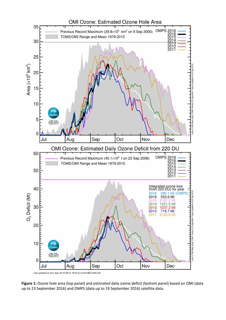
Figure 1: Ozone hole area (top panel) and estimated daily ozone deficit (bottom panel) based on OMI (data up to 23 September 2016) and OMPS (data up to 19 September 2016) satellite data.

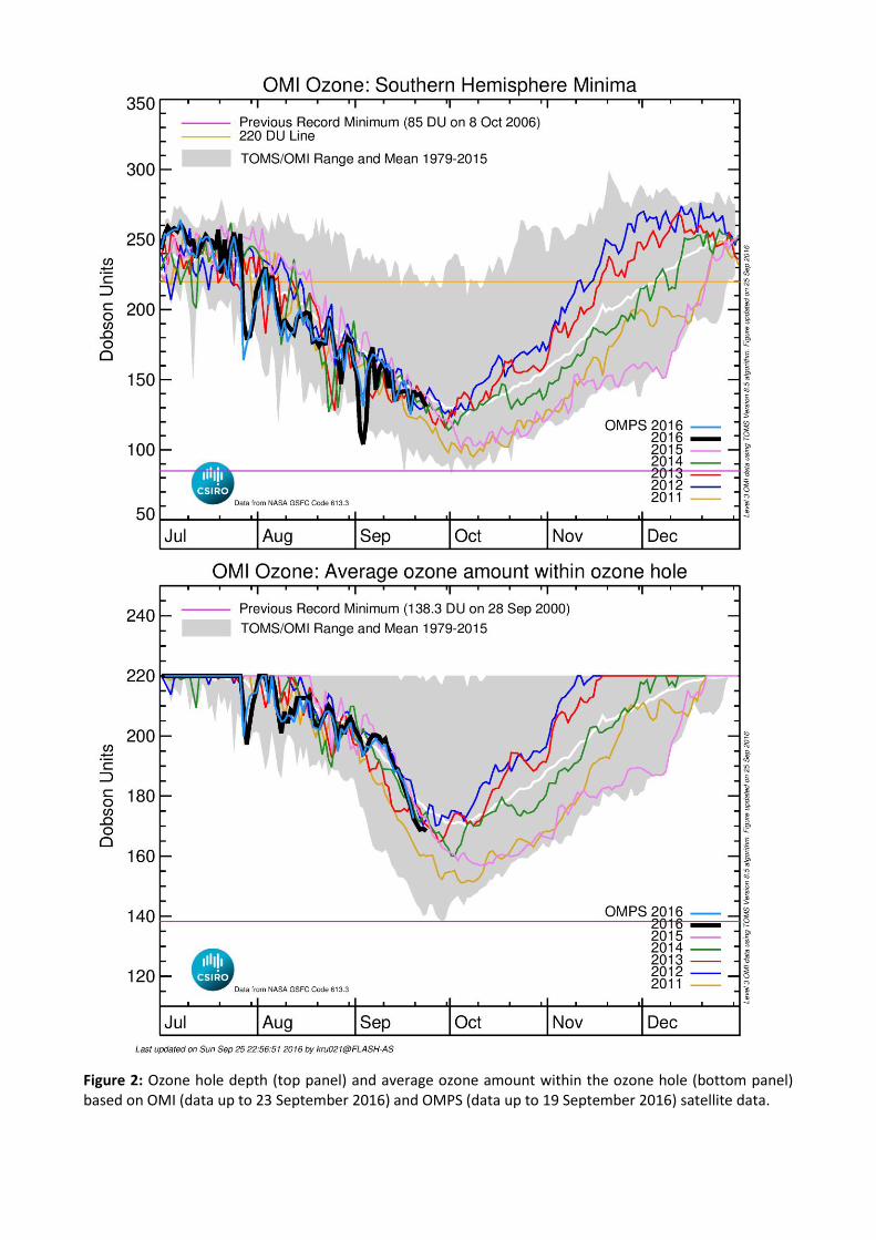
Figure 2: Ozone hole depth (top panel) and average ozone amount within the ozone hole (bottom panel) based on OMI (data up to 23 September 2016) and OMPS (data up to 19 September 2016) satellite data.

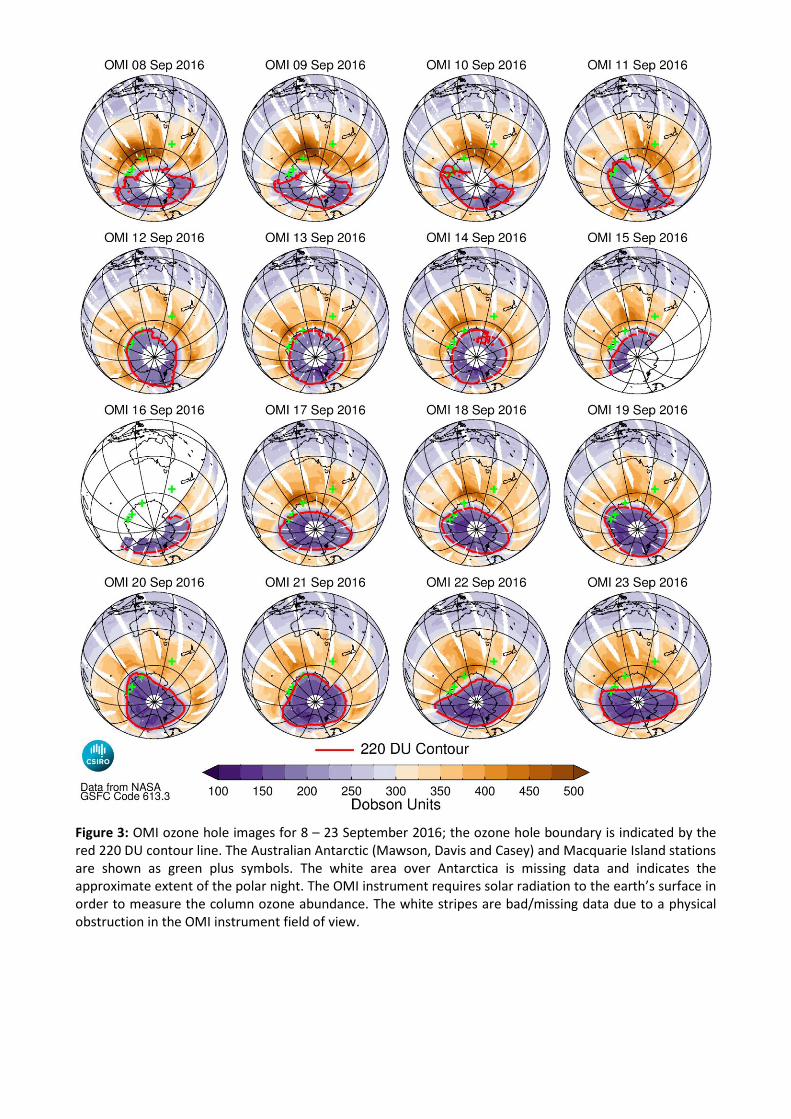
Figure 3: OMI ozone hole images for 8 – 23 September 2016; the ozone hole boundary is indicated by the red 220 DU contour line. The Australian Antarctic (Mawson, Davis and Casey) and Macquarie Island stations are shown as green plus symbols. The white area over Antarctica is missing data and indicates the approximate extent of the polar night. The OMI instrument requires solar radiation to the earth’s surface in order to measure the column ozone abundance. The white stripes are bad/missing data due to a physical obstruction in the OMI instrument field of view.

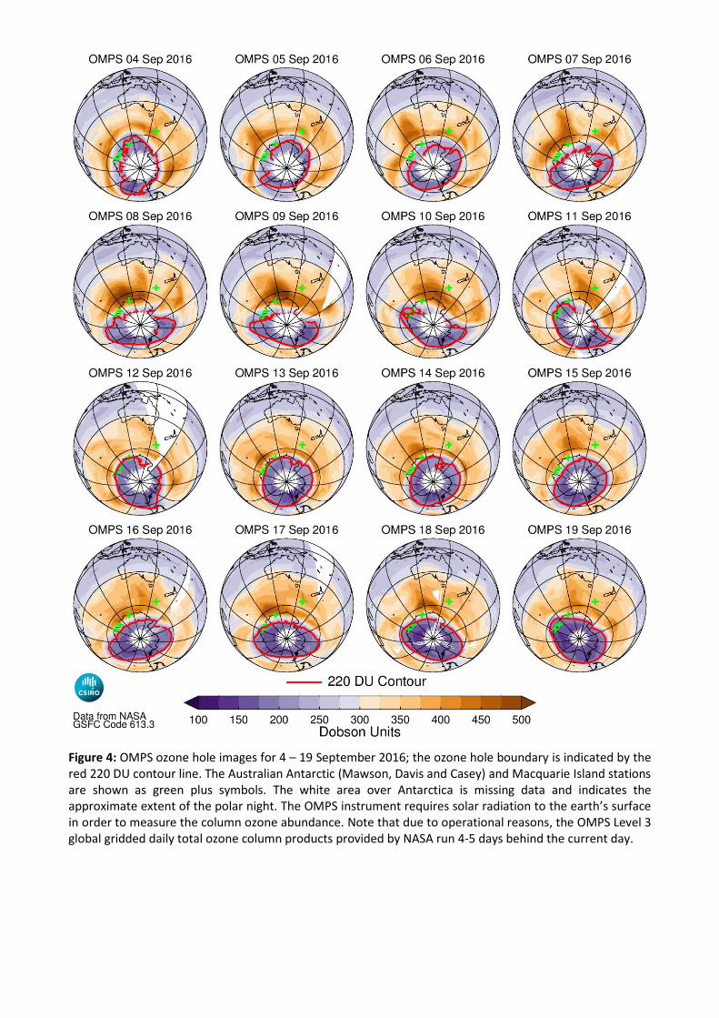
Figure 4: OMPS ozone hole images for 4 – 19 September 2016; the ozone hole boundary is indicated by the red 220 DU contour line. The Australian Antarctic (Mawson, Davis and Casey) and Macquarie Island stations are shown as green plus symbols. The white area over Antarctica is missing data and indicates the approximate extent of the polar night. The OMPS instrument requires solar radiation to the earth’s surface in order to measure the column ozone abundance. Note that due to operational reasons, the OMPS Level 3 global gridded daily total ozone column products provided by NASA run 4-5 days behind the current day.

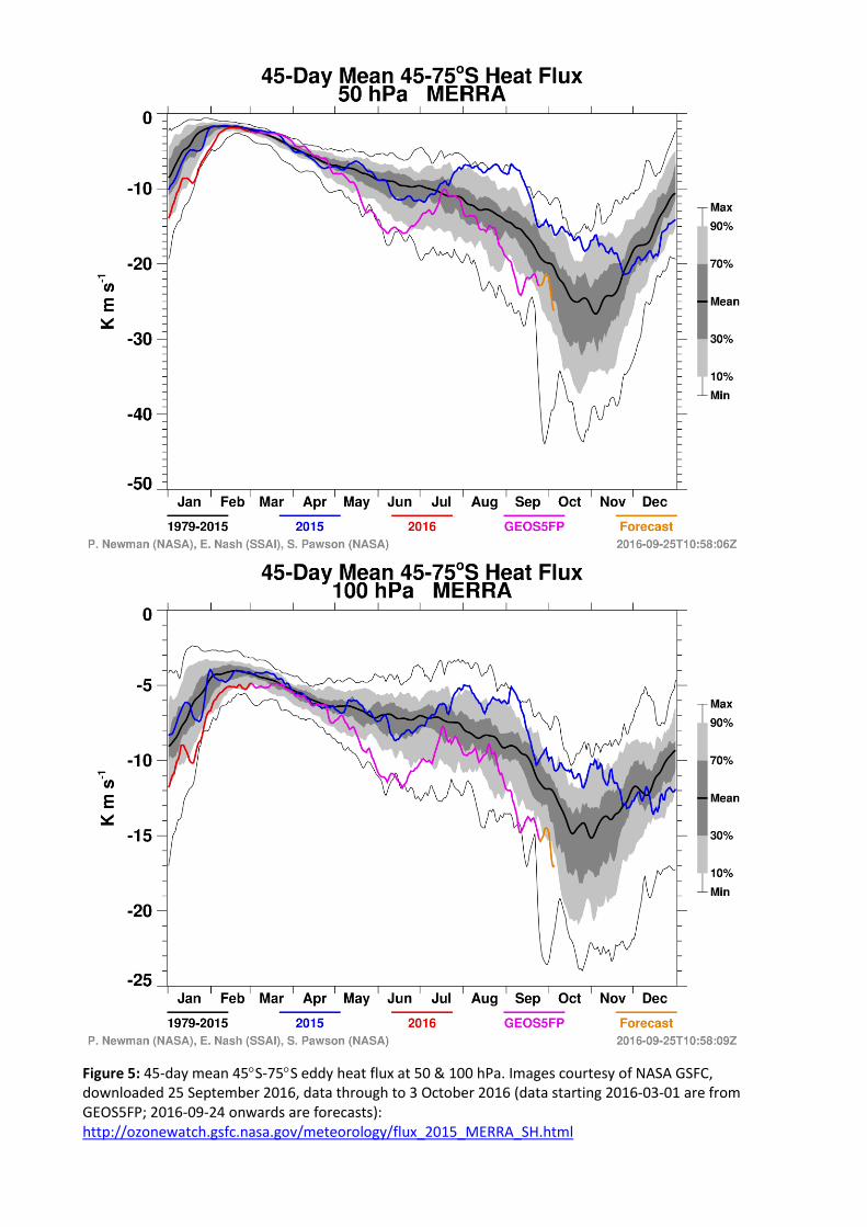
Figure 5: 45-day mean 45S-75S eddy heat flux at 50 & 100 hPa. Images courtesy of NASA GSFC, downloaded 25 September 2016, data through to 3 October 2016 (data starting 2016-03-01 are from GEOS5FP; 2016-09-24 onwards are forecasts): http://ozonewatch.gsfc.nasa.gov/meteorology/flux_2015_MERRA_SH.html

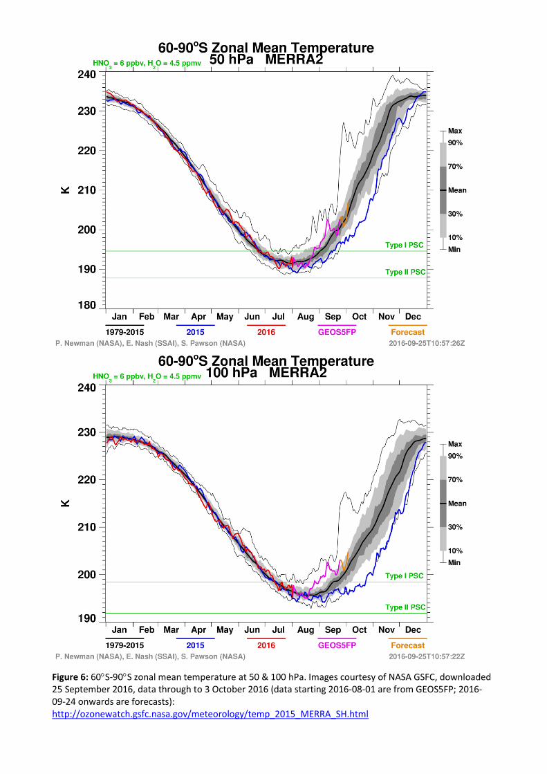
Figure 6: 60S-90S zonal mean temperature at 50 & 100 hPa. Images courtesy of NASA GSFC, downloaded 25 September 2016, data through to 3 October 2016 (data starting 2016-08-01 are from GEOS5FP; 2016-09-24 onwards are forecasts): http://ozonewatch.gsfc.nasa.gov/meteorology/temp_2015_MERRA_SH.html

Satellite Instrumentation

OMI

Data from the Ozone Monitoring Instrument (OMI) on board the Earth Observing Satellite (EOS) Aura, that have been processed with the NASA TOMS Version 8.5 algorithm, have been utilized again this year in our weekly ozone hole reports. OMI continues the NASA TOMS satellite record for total ozone and other atmospheric parameters related to ozone chemistry and climate.

On 19 April 2012 a reprocessed version of the complete (to date) OMI Level 3 gridded data was released. This is a result of a post-processing of the L1B data due to changed OMI row anomaly behaviour (see below) and consequently followed by a re-processing of all the L2 and higher data. These new data have now been reprocessed by CSIRO, which has resulted in small changes in the ozone hole metrics we calculate, and as such, these metrics may be slightly different for previous years for OMI data (2005-2011).

In 2008, stripes of bad data began to appear in the OMI products apparently caused by a small physical obstruction in the OMI instrument field of view and is referred to as a row anomaly. NASA scientists guess that some of the reflective Mylar that wraps the instrument to provide thermal protection has torn and is intruding into the field of view. On 24 January 2009 the obstruction suddenly increased and now partially blocks an increased fraction of the field of view for certain Aura orbits and exhibits a more dynamic behaviour than before, which led to the larger stripes of bad data in the OMI images. Since 5 July 2011, the row anomaly that manifested itself on 24 January 2009 now affects all Aura orbits, which can be seen as thick white stripes of bad data in the OMI total column ozone images. It is now thought that the row anomaly problem may have started and developed gradually since as early as mid-2006. Despite various attempts, it turned out that due to the complex nature of the row anomaly it is not possible to correct the L1B data with sufficient accuracy (≤ 1%) for the errors caused by the row anomaly, which has ultimately resulted in the affected data being flagged and removed from higher level data products (such as the daily averaged global gridded level 3 data used here for the images and metrics calculations). However, once the polar night reduces enough then this should not be an issue for determining ozone hole metrics, as there is more overlap of the satellite passes at the polar regions which essentially ‘fills-in’ these missing data.

OMPS

OMPS (Ozone Mapping and Profiler Suite) is a new ozone instrument on the Suomi National Polar-orbiting Partnership satellite (Suomi NPP), which was launched on 28 October 2011 and placed into a sun-synchronous orbit 824 km above the Earth. The partnership is between NASA, NOAA and DoD (Department of Defense), see http://npp.gsfc.nasa.gov/ for more details. OMPS will continue the US program for monitoring the Earth's ozone layer using advanced hyperspectral instruments that measure sunlight in the ultraviolet and visible, backscattered from the Earth's atmosphere, and will contribute to observing the recovery of the ozone layer in coming years. For the 2014 ozone hole season, we will also be using the OMPS total column ozone data by producing metrics from both OMI and OMPS Level 3 global gridded daily total ozone column products from NASA, and present both sets of results for comparison. NOTE that NASA receive the raw OMPS data from NOAA, and due to some operational delays, NASA have decided to delay the processing of data by 96 hours (4 days) from the time they obtain the first raw data for a given day. As a result, the OMPS Level 3 global gridded daily total ozone column products provided by NASA run 4-5 days behind the current day.

Archive of the Weekly Reports

The weekly Antarctic Ozone Hole reports for the 2016 ozone hole season are available from the Department of the Environment and Energy web page here:

http://www.environment.gov.au/protection/ozone/publications/antarctic-ozone-hole-summary-reports

Definitions

CFCs: chlorofluorocarbons, synthetic chemicals containing chlorine, once used as refrigerants, aerosol propellants and foam-blowing agents, that break down in the stratosphere (15-30 km above the earth’s surface), releasing reactive chlorine radicals that catalytically destroy stratospheric ozone.

DU: Dobson Unit, a measure of the total ozone amount in a column of the atmosphere, from the earth’s surface to the upper atmosphere, 90% of which resides in the stratosphere at 15 to 30 km.

Halons: synthetic chemicals containing bromine, once used as fire-fighting agents that break down in the stratosphere releasing reactive bromine radicals that catalytically destroy stratospheric ozone. Bromine radicals are about 50 times more effective than chlorine radicals in catalytic ozone destruction.

MERRA: is a NASA reanalysis for the satellite era using a major new version of the Goddard Earth Observing System Data Assimilation System Version 5 (GEOS-5). The project focuses on historical analyses of the hydrological cycle in a broad range of weather and climate time scales. It places modern observing systems (such as EOS suite of observations) in a climate context. Since these data are from a reanalysis, they are not up-to-date. So, NASA supplement with the GEOS-5 FP data that are also produced by the GEOS-5 model in near real time. These products are produced by the NASA Global Modeling and Assimilation Office (GMAO).

Ozone: a reactive form of oxygen with the chemical formula O3; ozone absorbs most of the UV radiation from the sun before it can reach the earth’s surface.

Ozone Hole: ozone holes are examples of severe ozone loss brought about by the presence of ozone depleting chlorine and bromine radicals, whose levels are enhanced by the presence of PSCs (polar stratospheric clouds), usually within the Antarctic polar vortex. The chlorine and bromine radicals result from the breakdown of CFCs and halons in the stratosphere. Smaller ozone holes have been observed within the weaker Arctic polar vortex.

Polar night terminator: the delimiter between the polar night (continual darkness during winter over the Antarctic) and the encroaching sunlight. By the first week of October the polar night has ended at the South Pole.

Polar vortex: a region of the polar stratosphere isolated from the rest of the stratosphere by high west-east wind jets centred at about 60°S that develop during the polar night. The isolation from the rest of the atmosphere and the absence of solar radiation results in very low temperatures (< -78°C) inside the vortex.

PSCs: polar stratospheric clouds are formed when the temperatures in the stratosphere drop below -78°C, usually inside the polar vortex. This causes the low levels of water vapour present to freeze, forming ice crystals and usually incorporates nitrate or sulphate anions.

TOMS, OMI & OMPS: the Total Ozone Mapping Spectrometer (TOMS), Ozone Monitoring Instrument (OMI), and Ozone Mapping and Profiler Suite (OMPS) are satellite borne instruments that measure the amount of back-scattered solar UV radiation absorbed by ozone in the atmosphere; the amount of UV absorbed is proportional to the amount of ozone present in the atmosphere.

UV radiation: a component of the solar radiation spectrum with wavelengths shorter than those of visible light; most solar UV radiation is absorbed by ozone in the stratosphere; some UV radiation reaches the earth’s surface, in particular UV-B which has been implicated in serious health effects for humans and animals; the wavelength range of UV-B is 280-315 nanometres.

Acknowledgements

The TOMS and OMI data are provided by the TOMS ozone processing team, NASA Goddard Space Flight Center, Atmospheric Chemistry & Dynamics Branch, Code 613.3. The OMI instrument was developed and built by the Netherlands's Agency for Aerospace Programs (NIVR) in collaboration with the Finnish Meteorological Institute (FMI) and NASA. The OMI science team is lead by the Royal Netherlands Meteorological Institute (KNMI) and NASA. The OMPS Level 3 data used in this report were created from a research dataset developed by NASA's NPP Ozone Science Team using nadir measurements from Suomi-NPP's Ozone Mapping and Profiler Suite(OMPS). All data were downloaded from ftp://jwocky.gsfc.nasa.gov/pub.